Incorporating Indirect Effects in Audit Case Selection: An Agent-Based Approach

Kim Michael Bloomquist, IRS Office of Research1

In selecting tax returns for its examination program the IRS historically has focused primarily on direct revenue maximization. According to Plumley and Steuerle (2004), “The appeal of direct revenue maxi-mization is that, for the most part, it is measurable, and it provides a basis for making resource allocation

decisions.” However, Plumley and Steuerle (2004, page 329) also point out that by relying on direct revenue maximization the IRS “views enforcement in isolation from voluntary compliance. To the extent that IRS ac-tivities—whether enforcement or non-enforcement—indirectly affect the voluntary compliance of the general population, it is the combination of direct and indirect revenue that is important.”

Bloomquist (2004) defines three types of indirect effects: induced, subsequent period, and group effects. Induced effects refer to a change in compliance behavior due to a change in enforcement level (e.g., audit rate or penalty rate). Thus, induced effects are analogous to the concept of probability of detection in the classic Allingham and Sandmo (1972) model of taxpayer reporting compliance. An example of induced effects would be if voluntary reporting compliance fell because IRS announced it was cutting 5,000 enforcement staff posi-tions. Subsequent period effects refer to a change in an individual taxpayer’s compliance behavior due to a prior tax audit. The first-hand experience of being audited reveals specific information to taxpayers about which issues the tax agency is interested in and how much it knows about taxpayers’ finances. With this additional in-formation, taxpayers may decide to increase or decrease their compliance (Gemmell and Ratto 2012). Finally, group effects are changes in compliance (also potentially in a positive or negative direction) by members of taxpayer j’s social network that can be attributed to communication with taxpayer j about his or her recent tax audit (Fortin, Lacroix, and Villeval 2007; Alm, Jackson, and McKee 2009). In this paper the term indirect effects refers to subsequent period and group effects only since tax agency resource levels are assumed to be fixed.

Indirect effects must be quantified if they are to be used in selecting tax returns to audit. The few stud-ies that have looked at this issue find that tax audits produce positive indirect effects ranging in magnitude from $6 for every $1 detected by examiners (Dubin, Graetz, and Wilde 1990) up to $11.60 (Plumley 1996).2 However, at best this research only tells us the average marginal indirect effect at a given point in time (or, for studies that rely on pooled time-series data, the average marginal indirect effect for the period of study). In order to incorporate indirect effects into the audit selection process we need to be able to model these, along with direct effects, at the level of the individual taxpayer.

A study by Long and Schwartz (1987) identified a group of taxpayers who were first subject to a Taxpayer Compliance Measurement Program (TCMP) audit of their 1969 tax returns and also selected for a TCMP audit in 1971. The authors found that the prior audit had a marginal impact on reducing the frequency of subsequent noncompliance, but not on the average magnitude of noncompliance of those taxpayers who were noncompliant in both years. However, since the initial TCMP audit experience was the result of random selection, it is possible that taxpayers did not respond in the same way they would if the first audit had been a “normal” operational audit (Andreoni, Erard, and Feinstein 1998). Erard (1992) analyzed reporting com-pliance for a group of taxpayers in the 1982 TCMP study who had been selected for an operational audit in 1980. He was unable to conclusively demonstrate that prior operational audits changed subsequent reporting behavior. However, Erard was able to show that this finding was sensitive to the method used to correct for sample selection bias.

Recently, Gemmell and Ratto (2012) find that random taxpayer audits can produce both negative and positive compliance effects depending on audit outcome and taxpayers’ opportunity to underreport. Using

Bloomquist104

a difference-in-differences approach, the authors investigate a group of UK taxpayers selected for a random audit in the year 2000 versus a control group of unaudited taxpayers. They observed taxpayers who were found to be compliant during the audit are more likely to report lower tax amounts during the 3 years following the audit (relative to the control group). The authors attribute this change in behavior to taxpayers lowering their expected audit probability (and expected detection rate) during the period under study. In contrast, taxpayers found to be noncompliant were more likely to increase reported taxes (relative to the control group). Again, the authors reasoned this change in behavior was linked to an increase in taxpayers’ perception of audit vul-nerability.

While more research is needed to understand and quantify the indirect effect of audits,3 a substantial body of knowledge on taxpayer compliance behavior has been built over the years using data from a variety of sources including taxpayer random audits,4 field studies (Slemrod, Blumenthal, and Christian 2001), and laboratory experiments (Alm 2010). Using this information as a foothold we can build a computational model to investigate alternative audit selection strategies making explicit assumptions about taxpayer behavior. Such a model ideally would include both subsequent period and group effects. One approach with this capability is agent-based modeling and simulation (ABMS).

In this paper I describe the design and implementation of the Individual Reporting Compliance Model (IRCM), an agent-based model (ABM) that simulates the income tax reporting behavior of a community of 85,000 individual taxpayers. The model is programmed in Java using Repast Simphony (North et al. 2007), a software toolkit created specifically for building ABMs. The model design allows for new information about taxpayer behavior to be incorporated as such knowledge becomes available.

The outline for the rest of this paper is as follows. The next section gives an overview of the IRCM includ-ing scope, dataset construction, agents, model execution, and model validation and calibration. The following section presents a hypothetical case study demonstrating how IRCM can be used to evaluate alternative audit case selection strategies. The final section concludes and highlights topics for further research.

Overview of the Individual Reporting Compliance ModelScopeAs a “proof-of-concept” model, the decision was made to build an ABM for a small region. Two criteria were used to select the study area. First, the region should be as similar as possible to the nation with respect to key economic and demographic characteristics (e.g., age structure, industry structure, racial composition, per capita income, etc.). Such a region would likely be more representative of the tax compliance behavior of the entire taxpayer population and would facilitate model validation using NRP data. Second, the region must be small enough to model on a personal computer. Several candidate regions were screened based on these crite-ria. From these, a single county with nearly 85,000 individual filers in TY 2001 was selected.

Dataset ConstructionIn order to allow for independent verification and validation testing while preserving taxpayer anonymity, the model is implemented using a dataset of artificial taxpayers. The basic idea in creating a dataset of artificial taxpayers is to substitute cases in the 2001 Statistics of Income (SOI) Public Use File (PUF)5 for tax returns of actual taxpayers in the study area. Although most fields in the PUF are derived from tax forms, SOI modifies the data in order to protect the identity of individuals. The IRS Master File is the source for tax return data.

Both the Master File data for the study region and the PUF data are partitioned6 and a PUF record is selected to replace each taxpayer record in the Master File data.7 Table 1 compares the resulting dataset of arti-ficial taxpayers using the process described above to the Master File tax return data for the study area.

From Table 1 we can see that for the largest line items (e.g., wages, Schedule C income, taxable pension income, Schedule E income, deductions, exemptions, and total adjusted gross income (AGI)) there is close

Incorporating Indirect Effects in Audit Case Selection: An Agent-Based Approach 105

agreement in the number of returns with nonzero values and total dollar amount. The region contains 21 zones based on postal Zip Code zones. In 20 of 21 zones (not shown in Table 1), the percentage difference in Total AGI between the artificial and Master File data is in the low single digits (Bloomquist 2012).

Table 1. Comparison of Actual vs. Artificial Taxpayer Data for Study Region

Income Itemactual Data Artificial Data Percentage

Differencein SumsN (nonzero) Sum ($1,000) N (nonzero) Sum ($1,000)

Wages 72,058 2,744,170 71,773 2,738,049 -0.2

Taxable Interest 47,768 138,156 42,582 125,803 -8.9

Taxable Dividends 22,951 77,716 19,590 65,905 -15.2

State Tax Refunds 14,955 6,098 10,764 7,287 19.5

Alimony 238 2,748 155 2,071 -24.6

Schedule C Income 8,728 92,480 7,610 90,104 -2.6

Schedule D Income 17,636 95,117 14,520 89,043 -6.4

other Gains 930 81 690 802 887.6

Taxable IRA Income 6,820 68,681 5,315 59,328 -13.6

Taxable Pension Income 18,604 277,083 16,597 269,574 -2.7

Schedule E Income 8,769 116,042 7,185 120,370 3.7

Schedule F Income 1,143 1,154 841 2,252 95.2

Unemployment Compensation 6,203 19,783 4,774 15,311 -22.6

Taxable Social Security 8,461 73,374 7,821 68,003 -7.3

other Income 4,576 9,194 4,573 222 -97.6

Total AGI 84,842 3,695,035 84,846 3,635,509 -1.6

Deduction Amount 84,851 731,363 84,907 743,302 1.6

Exemption Amount 75,870 455,524 75,905 453,310 -0.5

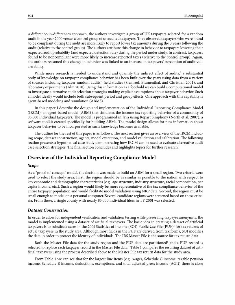
AgentsFigure 1 graphically displays the IRCM agent architecture. A single Region is composed of 21 nonoverlapping zones. Each Zone is assigned the actual number of filers who file tax returns from within its boundaries and also the number of tax preparers and employers that operate locally. A Preparer agent prepares tax returns for its clients. Employer agents have one or more employees. Both preparer-client and employer-employee rela-tionships are based on actual tax return data. Form 1040 filers are represented by Filer agents.

Finally, a single tax agency (an instance of the TaxAgency class) audits a fixed number of filers each tax pe-riod (simulation time step). The tax agency selects filers for audit using one of three audit strategies: random, fixed, or constrained maximum yield. In the latter case, the tax agency applies a simple learning algorithm to incrementally improve its overall yield per return audited.

Bloomquist106

FIgURe 1. IRCM agent Hierarchy

**

*

* *

21 Zones84,912 Filers

3,321 Employers2,129 Tax Preparers

*

Tax Agency

Employer

Region

Zone

Filer

Preparer

*

Model ExecutionThe steps followed in executing a simulation using IRCM are shown in Figure 2. The model first reads tax return data for the population of artificial taxpayers and instantiates agents. During instantiation, IRCM esti-mates a true amount for the most important Form 1040 income and offset items which is equal to the reported amount plus imputed misreporting.8 Imputed amounts are based on audit results from the TY 2001 NRP study. For 18 of the 19 imputed items9 an empirical Cumulative Distribution Function (ECDF) is created for each of the following four nonoverlapping groups of NRP cases: (1) self-prepared and zero reported amount, (2) self-prepared and nonzero reported amount, (3) paid prepared and zero reported amount and (4) paid prepared and nonzero reported amount. Next, a cubic function is fitted to each ECDF. During instantiation, the misreported amount for a line item is determined by drawing a random number from the interval [0, 1] and the misreported amount is generated using the cubic function for the appropriate preparation mode and reporting state.

Each time step represents one filing cycle (year). Tax calculations are performed twice for all taxpayers, once using reported amounts and a second pass using estimated true amounts. The difference in calculated tax using true and reported amounts is the tax gap for each filer. By default, IRCM assumes the difference between the true and reported tax amounts is the amount identified by the tax auditor. An option is provided to account for undetected underreporting by applying multipliers to the misreported amount detected by the examiner.10

Audits are performed at the next step. By default IRCM assumes audited tax returns are selected at ran-dom. An alternative to random selection is for the user to specify a fixed number of audits allocated among 17 mutually exclusive nonrandom audit classes (Table 2).

Incorporating Indirect Effects in Audit Case Selection: An Agent-Based Approach 107

Start

Instantiate Agents

Read Data

Time Loop

Calculate Tax

Tax Calculator Loop

Perform Audits

Process Stop FilersIssue AUR Notices

Update Learning BehaviorWrap Up p gUpdate Tax Agency Audit Targeting

Collect Statistics

Wrap Up

Generate Tables & Charts

End

FIgURe 2. IRCM execution Sequence: Top-level View

Bloomquist108

audit Class* Deduction Type business Unit Income Category Preparation Mode

1 Standard SB/SE TPI<100K Self

2 Standard SB/SE TPI<100K Paid

3 Standard SB/SE TPI>=100K Self

4 Standard SB/SE TPI>=100K Paid

5 Standard W&I TPI<100K Self

6 Standard W&I TPI<100K Paid

7 Standard W&I TPI>=100K Self

8 Standard W&I TPI>=100K Paid

9 Itemized SB/SE TPI<100K Self

10 Itemized SB/SE TPI<100K Paid

11 Itemized SB/SE TPI>=100K Self

12 Itemized SB/SE TPI>=100K Paid

13 Itemized W&I TPI<100K Self

14 Itemized W&I TPI<100K Paid

15 Itemized W&I TPI>=100K Self

16 Itemized W&I TPI>=100K Paid

17 Reported Taxable Income = 0

18 RandomNoTES: Standard = standard deduction, Itemized = itemized deduction, SB/SE = Small Business / Self-Employed, W&I = Wage and Investment, TPI = Total Positive Income, Self = self preparer, Paid = paid preparer.

* For audit classes 1 through 16, taxable income >0.

A third audit selection strategy available in IRCM is constrained maximum yield (CMY). Under this strat-egy the user specifies a maximum coverage rate and a minimum number of audits for the 17 nonrandom audit classes as well as the percentage of returns to select randomly (if any). At each time step the model identifies the audit classes with the lowest and the highest average yield (average yield = tax collected / number of audits performed).11 The tax agency then randomly drops a single audit case from the class with the lowest average yield and randomly selects an additional tax return to audit from within the class with the highest average yield. This process continues until the user-specified minimum coverage (or zero audits) is reached. Once the minimum coverage is reached, the tax agency then reallocates a single audit from the second lowest yielding audit class. Similarly, if the user-specified maximum coverage rate is reached, then the tax agency reallocates audits to the second highest yielding strategy, and so on. This process continues until the user-specified num-ber of simulation time steps is completed.

Following Gemmell and Ratto (2012) a filer’s response to an audit is based on user-supplied probabilities that cover two mutually-exclusive states (the filer is either compliant or noncompliant) and four response cat-egories: perfect compliance, increase compliance, decrease compliance and no change. In addition, the user may optionally allow taxpayers to change their reporting behavior if someone in their network of coworkers or social acquaintances is audited.

During the wrap-up phase of the simulation the tax agency issues Automated Underreporter (AUR) no-tices to taxpayers who are not audited but where computer checking of tax returns against information docu-ments detects some underreporting.12 In addition, filers may stop filing either because they leave the region or no longer have an obligation to file. Each “stop filer” is replaced by a new filer having identical income and network relationships as the filer he replaces but with reporting behavior reset to baseline levels and no memory of a prior audit experience (or audits of reference group members, if that option is selected). The reporting behavior of filers who are not “stop filers” is also updated at each time step, as is the audit selection

Table 2. IRCM audit Classes

Incorporating Indirect Effects in Audit Case Selection: An Agent-Based Approach 109

strategy of the tax agency. Finally, data collection occurs during the wrap-up phase. When the user-specified number of time steps has been completed the model generates output in the form of tables and charts that can be reviewed and saved for further analysis.

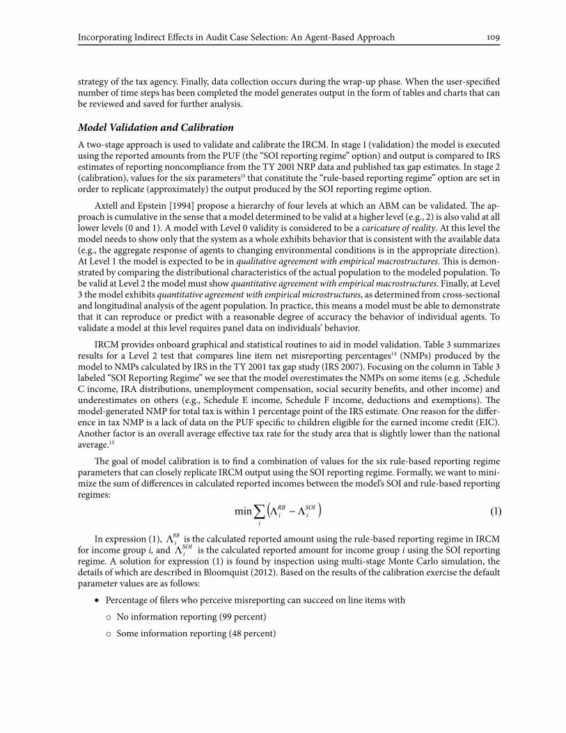
Model Validation and CalibrationA two-stage approach is used to validate and calibrate the IRCM. In stage 1 (validation) the model is executed using the reported amounts from the PUF (the “SOI reporting regime” option) and output is compared to IRS estimates of reporting noncompliance from the TY 2001 NRP data and published tax gap estimates. In stage 2 (calibration), values for the six parameters13 that constitute the “rule-based reporting regime” option are set in order to replicate (approximately) the output produced by the SOI reporting regime option.

Axtell and Epstein [1994] propose a hierarchy of four levels at which an ABM can be validated. The ap-proach is cumulative in the sense that a model determined to be valid at a higher level (e.g., 2) is also valid at all lower levels (0 and 1). A model with Level 0 validity is considered to be a caricature of reality. At this level the model needs to show only that the system as a whole exhibits behavior that is consistent with the available data (e.g., the aggregate response of agents to changing environmental conditions is in the appropriate direction). At Level 1 the model is expected to be in qualitative agreement with empirical macrostructures. This is demon-strated by comparing the distributional characteristics of the actual population to the modeled population. To be valid at Level 2 the model must show quantitative agreement with empirical macrostructures. Finally, at Level 3 the model exhibits quantitative agreement with empirical microstructures, as determined from cross-sectional and longitudinal analysis of the agent population. In practice, this means a model must be able to demonstrate that it can reproduce or predict with a reasonable degree of accuracy the behavior of individual agents. To validate a model at this level requires panel data on individuals’ behavior.

IRCM provides onboard graphical and statistical routines to aid in model validation. Table 3 summarizes results for a Level 2 test that compares line item net misreporting percentages14 (NMPs) produced by the model to NMPs calculated by IRS in the TY 2001 tax gap study (IRS 2007). Focusing on the column in Table 3 labeled “SOI Reporting Regime” we see that the model overestimates the NMPs on some items (e.g. ,Schedule C income, IRA distributions, unemployment compensation, social security benefits, and other income) and underestimates on others (e.g., Schedule E income, Schedule F income, deductions and exemptions). The model-generated NMP for total tax is within 1 percentage point of the IRS estimate. One reason for the differ-ence in tax NMP is a lack of data on the PUF specific to children eligible for the earned income credit (EIC). Another factor is an overall average effective tax rate for the study area that is slightly lower than the national average.15

The goal of model calibration is to find a combination of values for the six rule-based reporting regime parameters that can closely replicate IRCM output using the SOI reporting regime. Formally, we want to mini-mize the sum of differences in calculated reported incomes between the model’s SOI and rule-based reporting regimes:

In expression (1), RBiΛ is the calculated reported amount using the rule-based reporting regime in IRCM

for income group i, and SOIiΛ is the calculated reported amount for income group i using the SOI reporting

regime. A solution for expression (1) is found by inspection using multi-stage Monte Carlo simulation, the details of which are described in Bloomquist (2012). Based on the results of the calibration exercise the default parameter values are as follows:

• Percentage of filers who perceive misreporting can succeed on line items with

o No information reporting (99 percent)

o Some information reporting (48 percent)

( ) )1(min∑ Λ−Λi

SOIi

RBi

RB

Bloomquist110

o Substantial information reporting (10 percent)

• Marginal compliance impact of withholding on items with substantial information reporting (75 percent)

• Percentage of deontological filers (25 percent)

• De minimis reporting threshold on items with no information reporting ($1,000)

The last column in Table 3 shows line item NMPs produced by the model using the rule-based reporting regime option in IRCM with the above default parameter settings. The NMP for tax after refundable credits is a percentage point lower than the equivalent measure using the SOI reporting regime option. However, for most major line items (e.g., wages, Schedule C income, deductions, and exemptions) the NMP values are quite close.

Table 3. TY 2001 line Item NMPs: IRS vs. Model estimates for SoI and Rule-based Reporting Regimes1

Item IRS [2007](percentage)

Reporting Regime (percentage)

SoI Rule-based

Wages and salaries 1 1 1

Interest 4 3 5

Dividends 4 4 5

State income tax refunds 12 14 7

Schedule C 57 63 63

Schedule D 12 13 24

IRA distributions 4 7 4

Pensions and annuities 4 3 5

Schedule E 35 28 28

Schedule F 72 63 62

Unemployment Compensation 11 15 6

Social Security Benefits 6 10 5

other income 64 82 63

Taxable income 11 13 12

Tax 18 17 16

Adjustments -21 -24 -41

Deductions 5 3 5

Exemptions 5 4 51Model validation and calibration exercises were performed assuming no group effects and default values for subsequent period effects. The default values for subsequent period effects are set to the following values. When the filer is found to be compliant, the probability of decreasing compliance on items with some or no information report-ing is 50 percent and 50 percent no change in compliance. When the filer is found to be noncompliant, the probability of increasing compliance is 50 percent, the probability of decreasing compliance is 25 percent and 25 percent no change. See Gemmell and Ratto (2012) for a discussion of filers’ response to random tax audits. Values based on model output in Table 3 represent an average of five simulations using different random number seeds.

Source: IRS [2007, Figure 4] and IRCM output (Figure 21) at t=50.

Case StudyThis section presents a simulation experiment that shows how the IRCM can be used to assess the impact on taxpayer compliance of alternative audit case selection strategies. For this experiment the IRCM is executed using the rule-based reporting regime option with default values for the six parameters. In addition, the default values for subsequent period effects (see footnote 13) also are used. Finally, group effects are included by allow-ing filers to modify their reporting behavior based on the audit experiences of their neighbors and coworkers.

Incorporating Indirect Effects in Audit Case Selection: An Agent-Based Approach 111

It is assumed that if taxpayer j is audited then each of j’s neighbors or co-workers have a 25-percent chance of increasing their compliance, a 25-percent chance of decreasing their compliance and a 50-percent chance of no change.16 Both coworker and neighbor reference groups are assumed to have a fixed size of five members.17 For all other model options, including the number of audits (378) to perform, default values were used.

Four nonrandom audit selection strategies were defined for this example. They are:

1. CMY 100/0—Constrained Maximum Yield with a 100-percent maximum coverage rate and no minimum coverage

2. CMY 10/0—Constrained Maximum Yield with a 10-percent maximum coverage rate and no minimum coverage.

3. CMY 1/0—Constrained Maximum Yield with a 1-percent maximum coverage rate and no minimum coverage.

4. CMY 10/5—Constrained Maximum Yield with a 10-percent maximum coverage rate and a minimum of five audits in each audit class.

Each of these strategies was simulated five times using different seeds for IRCM’s random number genera-tor. Each simulation was run for 300 time steps. Figure 3 displays the time series of the average tax NMP from these five simulation runs for the four nonrandom audit selection strategies as well as a strategy based on pure random selection.

15.2%

15.4%

15.6%

14.4%

14.6%

14.8%

15.0%

NM

P

14.0%

14.2%

1 50 99 148 197 246 295

Time Step

CMY 100/0 CMY 10/0 CMY 1/0 CMY 10/5 Random

FIgURe 3. Model Time Series of Tax NMP for Five alternative audit Selection Strategies

Based on the plots displayed in Figure 3, the model reaches a stochastically stable solution for all strate-gies after about 250 time steps. Using the simulation output for the last 50 time steps, the pure random audit selection strategy has the highest tax NMP at 15.14 percent. The strategy with the next highest NMP is CMY 1/0 with 15.00 percent. The NMPs for the strategies CMY 10/0 and CMY 100/0 are quite close at 14.49 percent and 14.57 percent, respectively. The strategy with the lowest NMP (highest voluntary compliance) is CMY 10/5 with an NMP of 14.29 percent.

Table 4 compares the five audit selection strategies on the following measures: total estimated recom-mended audit results, total estimated misreported tax, and no change rate (i.e., the percentage of audit cases

Bloomquist112

with no recommended tax change). The deterrence multiplier is calculated as the reduction in misreported tax divided by the change in audit results. Table 4 shows that the strategy with the highest direct effect is CMY 100/0 with total recommended audit results of $2.991 million. However, the strategy with the highest com-bined direct and indirect effect is CMY 10/5 with total misreported tax of $89.789 million, an improvement of $1.228 million in additional tax revenue reported voluntarily over strategy CMY 100/0. The reason strategy CMY 10/5 produces a greater impact on voluntary compliance is due mainly to the influence of group effects. This is seen more clearly in Table 5, which displays the coverage rate and estimated recommended tax by audit class for the study area’s actual TY 2001 audits and the four simulated audit selection strategies.

Table 4. Comparison of alternative audit Case Selection Strategies

Strategyaudit Results ($1,000) Misreported Tax ($1,000)

Deterrence Multiplier

NoChange Rate (percentage)Total Change Total Reduction

Random 252 95,114 76.4

CMY 100/0 2,991 2,739 91,017 4,097 1.5 36.9

CMY 10/0 2,469 2,217 91,522 3,593 1.6 38.4

CMY 1/0 513 262 94,195 919 3.5 65.2

CMY 10/5 2,459 2,207 89,789 5,325 2.4 42.9

Table 5 shows that the strategies CMY 100/0 and CMY 10/0 select only tax returns that have income from a small business.18 The CMY 1/0 strategy is able to pick up some nonbusiness tax returns but the required low-er coverage of business audit classes reduces the likelihood of encountering cases with large recommended tax change amounts. The CMY 10/5 strategy is able to maintain sufficient high coverage of business audit classes while also having a net positive influence, via group effects, on the reporting compliance of nonbusiness filers.

ConclusionIn deciding which taxpayers to audit, the IRS ideally should take into account both direct and indirect ef-fects (Plumley and Steuerle 2004). However, the IRS has lacked a computational framework for systematically modeling indirect effects. This paper has addressed this methodological gap by introducing the Individual Reporting Compliance Model (IRCM). The IRCM is capable of performing a wide range of “what if ” analyses involving various aspects of taxpayer reporting compliance, including estimating the direct and indirect effects of taxpayer audits. This capability was demonstrated in a simulation experiment, which found that the audit strategy (of the four strategies analyzed) having the highest combined direct and indirect effect on voluntary reporting compliance was one with a relatively high coverage rate of business audit classes and a minimum coverage of nonbusiness audit classes.

As a proof-of-concept, the IRCM has demonstrated that agent-based simulation is able to incorporate many complexities of real-world tax systems, such as compliance differences at the line-item level and taxpay-ers’ heterogeneous response to audits, which have proven difficult for existing analytical models to handle simultaneously (Alm 1999). In addition to their ability to model complex systems, ABMs are able to explicitly incorporate taxpayer behavioral influences. The value of having such a capability grows as our knowledge of taxpayer behavior improves. Therefore, in order to achieve the maximum productive use of these new model-ing tools, the IRS must continue to invest in research on taxpayer behavior. Such research must necessarily ad-dress the complete array of cause-and-effect relationships between IRS service and enforcement activities and taxpayer compliance and burden, employing a range of data collection methodologies including laboratory experiments, field studies (including random and operational audits), and taxpayer surveys.

Incorporating Indirect Effects in Audit Case Selection: An Agent-Based Approach 113

Tab

le 5

. C

over

age

Rat

es a

nd e

xpec

ted

Tax

Yiel

d by

aud

it C

lass

: act

ual a

nd S

imul

atio

n R

esul

ts

aud

it C

lass

Tota

l R

etur

nsa

ctua

lN

onra

ndom

aud

it St

rate

gy

CM

Y 10

0/0

CM

Y 10

/0C

MY

1/0

CM

Y 10

/5

Cov

erag

eTa

x**

Cov

erag

eTa

xC

over

age

Tax

Cov

erag

eTa

xC

over

age

Tax

TI>0

, Std

Ded

, SB

, TP

I<10

0K, S

elf

2,49

00.

84%

$34,

800

0.00

%$4

470.

24%

$7,0

511.

00%

$28,

181

1.52

%$5

,474

TI>0

, Std

Ded

, SB

, TP

I<10

0K, P

aid

4,04

40.

72%

$202

,300

0.17

%$1

0,92

90.

59%

$38,

304

0.99

%$6

3,23

01.

30%

$11,

276

TI>0

, Std

Ded

, SB

, TP

I>10

0K, S

elf

78*

$1,5

0037

.18%

$109

,760

7.69

%$3

4,74

00.

00%

$03.

78%

$41,

465

TI>0

, Std

Ded

, SB

, TP

I>10

0K, P

aid

203

*$6

3,50

025

.62%

$271

,967

9.85

%$1

37,8

680.

00%

$04.

33%

$142

,141

TI>0

, Std

Ded

, WI,

TPI<

100K

, Sel

f32

,512

0.34

%$2

10,3

000.

00%

$00.

00%

$00.

00%

$00.

02%

$339

TI>0

, Std

Ded

, WI,

TPI<

100K

, Pai

d20

,784

0.63

%$3

11,8

000.

00%

$00.

00%

$00.

37%

$7,7

460.

03%

$442

TI>0

, Std

Ded

, WI,

TPI>

100K

, Sel

f20

5*

$00.

00%

$00.

00%

$00.

00%

$02.

45%

$3,3

97

TI>0

, Std

Ded

, WI,

TPI>

100K

, Pai

d17

0*

$00.

00%

$00.

00%

$00.

00%

$02.

96%

$6,0

82

TI>0

, Itm

Ded

, SB

, TP

I<10

0K, S

elf

1,74

00.

69%

$38,

100

0.17

%$4

,210

1.03

%$2

9,32

10.

98%

$26,

352

2.42

%$1

3,13

6

TI>0

, Itm

Ded

, SB

, TP

I<10

0K, P

aid

3,16

50.

76%

$52,

700

0.41

%$2

5,60

11.

45%

$94,

650

1.01

%$6

6,07

01.

99%

$54,

655

TI>0

, Itm

Ded

, SB

, TP

I>10

0K, S

elf

751

*$8

,600

4.66

%$1

52,7

429.

99%

$287

,522

1.01

%$3

2,47

64.

23%

$282

,869

TI>0

, Itm

Ded

, SB

, TP

I>10

0K, P

aid

1,83

71.

31%

$140

,900

13.0

1%$2

,415

,281

9.96

%$1

,839

,466

0.98

%$2

36,5

504.

37%

$1,8

61,4

34

TI>0

, Itm

Ded

, WI,

TPI<

100K

, Sel

f6,

839

*-$

2,30

00.

00%

$00.

00%

$00.

99%

$15,

525

0.10

%$1

,032

TI>0

, Itm

Ded

, WI,

TPI<

100K

, Pai

d6,

497

*$5

,600

0.00

%$0

0.00

%$0

0.98

%$1

4,37

20.

13%

$1,3

14

TI>0

, Itm

Ded

, WI,

TPI>

100K

, Sel

f1,

635

*$2

,300

0.00

%$0

0.00

%$0

0.96

%$1

0,37

90.

40%

$3,1

17

TI>0

, Itm

Ded

, WI,

TPI>

100K

, Pai

d1,

455

*-$

6,20

00.

00%

$00.

00%

$00.

94%

$12,

384

0.81

%$3

,510

TI<=

050

7*

$6,3

000.

00%

$00.

00%

$00.

00%

$00.

99%

$27,

431

Tota

l (ex

clud

es R

ando

m)

84,9

120.

45%

$1,0

70,2

000.

45%

$2,9

90,9

360.

45%

$2,4

68,9

220.

45%

$513

,265

0.45

%$2

,459

,113

*Few

er th

an 1

0 ob

serv

atio

ns.

**R

ound

ed to

nea

rest

$10

0.

Bloomquist114

ReferencesMichael G. Allingham and Agnar Sandmo. Income Tax Evasion: A Theoretical Analysis. Journal of Public

Economics, 1 (3/4):323–338, 1972.James Alm. Tax Compliance and Administration. In W. Bartley Hildreth and James A. Richardson, editors,

Handbook on Taxation, pages 741–68, New York, Mercel Dekker, 1999.James Alm. Testing Behavioral Public Economics Theories in the Laboratory. National Tax Journal,

63(4):635–658, 2010.James Alm, Betty R. Jackson, and Michael McKee. Getting the Word Out: Enforcement Information

Dissemination and Compliance Behavior. Journal of Public Economics, 93: 392–402, 2009.James Alm, Jorge Martinez-Vazquez, and Benno Torgler. Developing Alternative Frameworks for Explaining

Tax Compliance. Routledge, New York, 2010.James Andreoni, Brian Erard, and Jonathan Feinstein. Tax Compliance. Journal of Economic Literature, 36

(2):818–860, 1998.Robert L. Axtell and Joshua M. Epstein. Agent-Based Modeling: Understanding Our Creations. The Bulletin

of the Santa Fe Institute, 28–32, 1994.Kim Michael Bloomquist. Multi-Agent Based Simulation of the Deterrent Effects of Taxpayer Audits.

National Tax Association Proceedings, Ninety-Seventh Annual Conference: 159–173, 2004.Kim Michael Bloomquist. Agent-Based Simulation of Tax Reporting Compliance. Unpublished doctoral

dissertation in Computational Social Science, George Mason University, Fairfax, Virginia. 2012.Robert E. Brown and Mark J. Mazur. IRS’s Comprehensive Approach to Compliance Measurement. National

Tax Journal, 56(3):689–700, 2003.Jeffrey A. Dubin, Michael J. Graetz, and Louis L. Wilde. The Effect of Audit Rates on the Federal Individual

Income Tax, 1977–1986. National Tax Journal, 43:395–409, 1990.Brian Erard. The Influence of Tax Audits on Reporting Behavior. In Joel Slemrod, editor, Why People Pay

Taxes, The University of Michigan Press, Ann Arbor, MI, 1992.Brian Erard and Jonathan S. Feinstein. The Individual Income Reporting Gap: What We See and What We

Don’t. Paper Prepared for IRS-TPC Research Conference on New Perspectives in Tax Administration, June 22, 2011.

Bernard Fortin, Guy Lacroix, and Marie Claire Villeval. Tax Evasion and Social Interactions. Journal of Public Economics, 91:2089-2112, 2007.

Norman Gemmell and Marisa Ratto. Behavioral Responses to Taxpayer Audits: Evidence from Random Taxpayer Inquiries. National Tax Journal, 65 (1):33–58, 2012.

Internal Revenue Service. Reducing the Federal Tax Gap: A Report on Improving Voluntary Compliance. Available at http://www.irs.gov/pub/irs-news/tax_gap_report_final_080207_linked.pdf. August 2, 2007.

Susan B. Long and Richard D. Schwartz. The Impact of IRS Audits on Taxpayer Compliance: A Field Experiment in Specific Deterrence. Paper presented at the annual meeting of the Law and Society Association. Washington, D.C. 1987.

Michael J. North, Eric Tatara, N.T. Collier, and J. Ozik. Visual Agent-Based Model Development with Repast Simphony. Proceedings of the 2007 Conference on Complex Interaction and Social Emergence, Argonne National Laboratory, Argonne, IL USA, 2007.

Alan H. Plumley. The Determinants of Individual Income Tax Compliance: Estimating the Impacts of Tax Policy, Enforcement, and IRS Responsiveness. Internal Revenue Service Publication 1916 (Rev. 11-96), Washington, D.C., 1996.

Incorporating Indirect Effects in Audit Case Selection: An Agent-Based Approach 115

Alan H. Plumley and C. Eugene Steuerle. Ultimate Objectives for the IRS: Balancing Revenue and Service. In Henry J. Aaron and Joel Slemrod, editors, The Crisis in Tax Administration, Brookings Institution Press, 2004.

Joel Slemrod, Marsha Blumenthal, and Charles Christian. Taxpayer Response to an Increased Probability of an Audit: Evidence from a Controlled Experiment in Minnesota. Journal of Public Economics, 79:455–483, March 2001.

United States Government Accountability Office. Tax Gap: IRS Could Significantly Increase Revenues by Better Targeting Enforcement Resources, GAO Report Number 13–151, December 2012.

Michael Weber. General Description Booklet for the 2001 Public Use Tax File. Individual Statistics Branch, Statistics of Income Division, Internal Revenue Service, October 2004.

Endnotes1 The content of this paper reflects the views of the author and does not necessarily represent the position of

the Internal Revenue Service.2 These estimates of the indirect effects of audits implicitly include induced, subsequent period, and group

effects. Summaries of empirical research on the indirect effect of audits is found in Andreoni, Erard, and Feinstein (1998) and Alm, Jackson and McKee (2009).

3 Although the focus of this paper is on audit case selection, the need for more research on the compliance impact of other IRS service and enforcement programs exists as well. In fact, the impact on compliance of nonaudit programs together or even separately may be greater than operational audits alone. See Plumley (1996) for an empirical analysis of the impact on filing and reporting compliance of different IRS enforcement and service measures.

4 In the U.S., the IRS National Research Program (NRP) annually selects a stratified random sample of about 13,000 tax returns for compliance assessment purposes (Brown and Mazur 2003). The phrase “random audits” or “taxpayer random audits” as used in this paper refers to audits of this type.

5 The 2001 PUF (Weber 2004) is a stratified probability sample containing records for 143,221 tax returns.6 Partitions represent a unique combination of filing status (Single, Married Filing Joint/Qualifying

Widow(er), Married Filing Separate, Head of Household), deduction type (itemized or standard deduction), wage income exceeding 50 percent of adjusted gross income (AGI) (in absolute value), AGI > median AGI by filing status, and presence of one or more exemptions for children at home.

7 The selected PUF record is drawn from the same partition as the Master File record and minimizes the Minkowski distance based on Form 1040 income line items as well as the deduction and exemption amounts. Restricting cases to matching partitions improves the overall agreement between the actual and artificial taxpayer datasets by ensuring the same filing status profile and presence of exemptions.

8 Imputed income items are: wages, interest, dividends, State tax refunds, alimony, sole proprietor income (Schedule C), capital gains income (Schedule D), other gains (Form 4797), individual retirement account (IRA) income, pension income, supplemental income (Schedule E), farm income (Schedule F), unemployment compensation, social security, and other income. Imputed offset items are: adjustments, deductions, exemptions and statutory credits (net the Child Tax Credit). Adjustments to certain credits (e.g., Child Tax Credit, Earned Income Credit, and Additional Child Tax Credit) that reflect a change in income are performed by a tax calculator. Each tax return consists of 180 elements based on the PUF data.

9 Imputed misreported exemptions are based on the probability of a change in number of exemptions from the TY 2001 NRP study.

10 Multipliers are applied to positive misreported amounts; that is, misreporting in the taxpayer’s favor. An overview of the DCE methodology and a description of the multipliers used by IRCM are found in Erard and Feinstein (2011). This approach follows the methodology used by IRS to estimate the tax gap for TY 2001 and prior years. In its most recent tax gap estimate for TY 2006, the IRS began to impute additional income to individuals who had zero detected noncompliance. The difference in the overall tax gap calculated between these two approaches is within the margin of error. However, the more recent

Bloomquist116

imputation methodology is preferable since it explicitly assumes the statistical nature of estimates of undetected underreporting.

11 In this paper the approach for selecting tax returns uses average yields for operational tractability. An alternative paradigm based on marginal yields is preferred on theoretical grounds by economists. However, there are practical obstacles to implementing a return selection algorithm based on marginal yields including: (a) the uncertainty associated with predicting direct yields from individual tax returns; and (b) the heterogeneous, stochastic, and time-variant nature of indirect effects. Moreover, to date, proposals to base return selection on marginal yields have been limited to consideration of direct effects only (see U.S. GAO 2012). Since the main focus of this paper is how to incorporate indirect effects in return selection, the author believes it is appropriate to base return selection on average yields.

12 The threshold amount for issuing an AUR notice is set by the user. The default value is $1.13 The six rule-based reporting regime parameters are: the percentage of filers that perceive misreporting can

succeed on line items with none, some, and substantial information reporting, the marginal compliance impact of tax withholding, the percentage of deontological filers, and the de minimis threshold amount for reporting. Deontological filers are filers who comply out of a sense of “duty” (Alm, Martinez-Vazquez, Torgler 2010) in contrast to the assumption of rational utility maximization (Allingham and Sandmo 1972).

14 The net misreporting percentage is defined as the aggregate net misreported amount expressed as a percentage of the sum of the absolute values of the amounts that should have been reported.

15 The nation’s estimated mean effective tax rate in TY01 is 14.95 percent versus 14.69 percent for the study region.

16 In IRCM reporting compliance can decrease on line items with some or no information reporting but not on items with substantial information reporting. Compliance is allowed to increase on all line items.

17 For employers with fewer than six employees but more than one employee, the coworker reference group size is N – 1 where N is the number of employees.

18 Small business income is defined as income reported on a Schedule C, Schedule F or Schedule E.