Embed Size (px)
Citation preview

1
Incorporating Agro-Ecologically Zoned Land Use Data and Land-
based Greenhouse Gases Emissions into the GTAP Framework
Huey-Lin Lee
Centre for Global Trade Analysis, Purdue University
Email: [email protected]
ABSTRACT
The paper describes the on-going project of the GTAP land use data base. We also
present the GTAPE-AEZ model, which illustrates how land use and land-based
emissions can be incorporated in the CGE framework for Integrated Assessment (IA)
of climate change policies. We follow the FAO fashion of agro-ecological zoning
(FAO, 2000; Fischer et al, 2002) to identify lands located in six zones. Lands located
in a specific AEZ have similar (or homogenous) soil, landform and climatic
characteristics. The six AEZs range over a spectrum of length of growing period
(LGP) for which their climate characteristics can support for crop growing. AEZ 1
covers the land of the temperature and moisture regime that is able to support length
of growing period (LGP) up to 60 days per annum. On the other end of the LGP
spectrum, lands in AEZ 6 can support a LGP from 270 to 360 days per annum. Crop
growing, livestock breeding, and timber plantation are dispersed on lands of each
AEZ of the six, whichever meets their climatic and edaphic requirements.
In GTAPE-AEZ, we assume that land located in a specific AEZ can be moved
only between sectors that the land is appropriate for their use. That is, land is mobile
between crop, livestock and forestry sectors within, but not across, AEZ’s. In the
2
standard GTAP model, land is assumed to be transformable between uses of crop
growing, livestock breeding, or timber plantation, regardless of climatic or soil
constraints. The fact is that most crops can only grow on lands that is under certain
temperature, moisture, soil type, land form, etc.. The same concern arises for land use
by the livestock and the forestry sectors. Lands that are suitable for growing wheat
may not be good for rice cultivation alike, even under transformation at a reasonable
cost. The introduction of the agro-ecological zoning in GTAP helps to clear up the
counterfactual assumption in inter-sectoral land transition, and permit a sound
presentation of sectoral competition for land.
Table of Contents:
1. Introduction............................................................................................................3
2. The AEZ-identified Land Use Data.......................................................................4
2.1 Agro-Ecological Zoning ............................................................................4
2.2 The GTAP Land Use Data Base ................................................................5
3. GTAP Greenhouse Gases Emissions Data ..........................................................15
3.1 CO2...........................................................................................................15
3.2 Non-CO2 greenhouse gases......................................................................15
4. A brief overview of the GTAPE-AEZ model ......................................................18
5. An Illustrative Simulations ..................................................................................24
5.1 Marginal abatement cost curves...............................................................26
5.2 Land transitions between uses under a 10% reduction of all GHGs........28
6. Concluding remarks and future research agenda .................................................30

3
1. Introduction
Land use, land-use change and forestry (LULUCF) activities have been perceived as a
relatively cost-effective option to mitigate climate change due to the rapid buildup of
greenhouse gases (GHGs) in the atmosphere. LULUCF may contribute to abatement
of emissions by increasing carbon storage in forests (the so-called sinks: enhancing
afforestation and forest management, while curbing deforestation). Article 3 of the
Kyoto Protocol makes provision for the Annex I parties to take into account removals
and emissions due to LULUCF activities since 1990 (e.g., afforestation, reforestation,
deforestation and other agreed land use changes) to meet their commitment targets of
greenhouse gas emission abatement. In the seventh Conference of the Parties (COP7)
to the UNFCCC held in Marrakesh, October/November 2001, the parties finally
agreed to include land-based carbon sequestration in their 2008-2012 GHG emissions
reduction targets. The COP9, held in Milan, December 2003, has reached consensus
for the rules of accounting for LULUCF projects in the Clean Development
Mechanism (CDM) for the first commitment period (2008-2012) of the Kyoto
Protocol. Along with such policy commitments, research on Integrated Assessment
(IA) of climate change has recently been advancing towards the LULUCF embraced
analysis.
At the 2002 MIT workshop (GTAP Website, 2002), co-sponsored by the U.S.
Environmental Protection Agency (US-EPA), Massachusetts Institute of Technology
(MIT), and the Center for Global Trade Analysis (GTAP), the idea of identifying
agro-ecological zoning in the GTAP model (Hertel, 1997) was sparked in the
discussion among the participating experts. The recognition of various agro-
ecological zones (AEZ) is believed to be a more realistic approach in modeling land
use change in GTAP, where land is mobile between crop, livestock and forestry
4
sectors within, but not across, AEZ’s. In the standard GTAP model, land is assumed to
be transformable between uses of crop growing, livestock breeding, or timber
plantation, regardless of climatic or soil constraints. The fact is that most crops can
only grow on lands that is under certain temperature, moisture, soil type, land form,
etc.. The same concern arises for land use by the livestock and the forestry sectors.
Lands that are suitable for growing wheat may not be good for rice cultivation alike,
even under transformation at a reasonable cost. The introduction of the agro-
ecological zoning in GTAP helps to clear up the counterfactual assumption in inter-
sectoral land transition, and permit a sound presentation of sectoral competition for
land.
We follow the FAO fashion of agro-ecological zoning (FAO, 2000; Fischer et al,
2002) to identify lands located in six zones of different agro-ecological feature. In
section 2, we introduce the AEZ-identified land use data. In section 4, we introduce
the GTAPE-AEZ model, which is based on the GTAP-E model (Burniaux and Truong,
2001). GTAPE-AEZ identifies six agro-ecological zones (AEZ) for the U.S., China,
and rest of world. In Section 5, we present the selective results of the illustrative
simulation with the GTAPE-AEZ model on the economic impact of carbon tax under
the multi-gas mitigation scheme. Section 6 concludes the paper and points out future
research direction.
2. The AEZ-identified Land Use Data
2.1 Agro-Ecological Zoning
The Food and Agriculture Organization (FAO) of the United Nations and the
International Institute for Applied Systems Analysis (IIASA) pioneered in the Land
5
Use and Land Cover (LUC) project and have developed an agro-ecological zoning
methodology during the past 20 years. Agro-ecological zoning refers to segmentation
of a parcel of land into smaller units according to agro-ecological characteristics, e.g.,
moisture and temperature regimes, soil type, landform, etc. In other words, each zone
has a similar combination of constraints and potentials for land use. The FAO/IIASA
agro-ecological zoning methodology provides a standardized framework for
characterizing climate, soil and terrain conditions pertinent to agricultural production
(FAO and IIASA, 2000).
The key concept of “length of growing period” (LGP) is brought in to differentiate
the agro-ecological zones by attainable crop productivity. The “length of growing
period” (LGP) refers to the period during the year when both soil moisture1 and
temperature are conducive to crop growth. Thus, in a formal sense, LGP refers to the
number of days within the period of temperatures above 5°C when moisture
conditions are considered adequate (FAO, 2000).
2.2 The GTAP Land Use Data Base
Outlook of the GTAP land use data
In constructing the GTAP land use data base, we adopt the FAO/IIASA convention of
agro-ecological zoning. Figure 1 shows the format of the GTAP land use data, which
is proposed at the 2002 MIT workshop (GTAP Website, 2002). We identify land
located in various agro-ecological zones (the rows in Figure 1) and the uses (sectors
or activities) of land (the columns in Figure 1).
1 Soil moisture is a function of precipitation, soil type, topography, etc.

6
Land use types in region r
AEZs Crop1 …. CropN Livestock1 …. LivestockH Forest1 …. Forestv
AEZ1
….
….
AEZM
Total
Figure 1. GTAP land use matrix
Acreage and production data by AEZ
The GTAP AEZ-specific land use data are compiled from a set of land acreage and
production provided by Dr. Navin Ramancutty of the Center for Sustainability and
Global Environment (SAGE), University of Wisconsin-Madison, for the cropland and
pasture land; and by Dr. Brent Sohngen of Ohio State University, for the forest land.
The SAGE data cover 19 crops and 3 species of timber located in 18 agro-ecological
zones (6 AEZs coupled with 3 climate zones—boreal, temperate, tropical). The 6
AEZs in the SAGE data follow the FAO/IIASA methodology of agro-ecological
zoning. The 6 AEZs range over a spectrum of length of growing period (LGP) for
which their climate characteristics can support for crop growing. AEZ 1 covers the
land of the temperature and moisture regime that is able to support length of growing
period (LGP) up to 60 days per annum. Lands in AEZ 2 can support LGP of 61 to 120
days per annum. On the other end of the LGP spectrum, lands in AEZ 6 can support a
LGP from 270 to 360 days per annum. Figure 2 shows the SAGE global map of the
18 AEZs, by 0.5 degree grid cell. Table 3 shows the cropland distribution of China, as
provided by SAGE. This table contains the harvested area data. It indicates that most
of the crops are grown in temperate area (AEZs 7 to 12).

7
Harvested area v.s. physically cultivated area
When we split the GTAP sectoral land rents into AEZs, we thought we would need to
convert the harvested area data of SAGE to physically cultivated area data due to the
concern of multiple cropping. However, we later realize that we do not really need
physically cultivated area data. In the GTAP Input-Output data, land rents are
generated from the activity (or use) that is going on the given parcel of land during the
calendar year. Furthermore, the fact shows that farmers may grow more than one crop
on the same parcel of land at different intervals (or periods) of the calendar year. For
example, farmers grow early double-crop rice from March to July, and then grow
catch crops (e.g., vegetables) in the rest of the calendar year. As GTAP Input-Output
data identify sector in terms of crops (e.g., the paddy rice sector, the cereal grain
sector, the oil seeds sector, etc.), land rents of the crop sectors should accrue to the
harvested area, which represents the activity of the given crop sector on the given
parcel of land at certain interval of the year. In the abovementioned example, we
should allot the land rent generated due to the growing of paddy rice to the GTAP
paddy rice sector, and allot the land rent generated due to the growing of vegetables to
the GTAP vegetables sector. In this example, land rent is tied to the harvested area,
instead of the physically cultivated area. In addition, land based emissions (e.g., CH4
emissions from paddy rice cultivation) are mostly tied to the harvested area (IPCC
1996 Guidelines). Fertilizer use is normally proportional to harvested area. So, we
conclude that harvested area is the data we need to use for the GTAP land use data,
rather than the physically cultivated area.

8
GTAP cropland rent data by 18 AEZs
We split the GTAP sectoral land rents into 18 AEZs according to the AEZ-specific
production shares as derived from the data provided by SAGE and Sohngen. Table 4
shows the mapping between SAGE’s 19 crops to GTAP’s 8 crops. Equation 1 is the
formula we use to split the GTAP sectoral land rents into 18 AEZs (Lca). For region r,
Lca = Lc* [ ∑i∈ SAGECROPS=c
Pi*QiaHia*Hia / ∑
a∈ AEZS
∑i∈ SAGECROPS=c
Pi*QiaHia*Hia ],
c∈ CROPS; i∈ SAGECROPS; a∈ AEZS. (Eq. 1) where
Lca is the land rent accrued to GTAP crop sector c in AEZ a;
Lc is the land rent of GTAP crop sector c, with no AEZ distinction;
Pi is the per-ton price of SAGE’s crop i;
Qia is the production (ton) of SAGE’s crop i in AEZ a; and
Hia is the harvested area of SAGE’s crop i in AEZ a.
Set SAGECROPS contains SAGE’s 19 crops;
set CROPS contains GTAP’s crops, which are more aggregated than SAGE’s.
Mapping CROP_SG2GT from SAGECROPS (index i) to CROPS (index c) (see
Table 4).
The ∑i∈ SAGECROPS=c
operator in Eq. 1 means to aggregate over disaggregated crops i to the
corresponding aggregated crop c.
Note that we assume the per-ton crop price (Pi) is homogenous across AEZs.
Data source of Lc = coefficients VFM and VDFA from the GTAP data base;
Data source of Pi = FAOSTAT;
Data source of Qia = tentatively self calculation based on SAGE's harvested area and
FAO's yield data; SAGE data will be available a couple of months later;
9
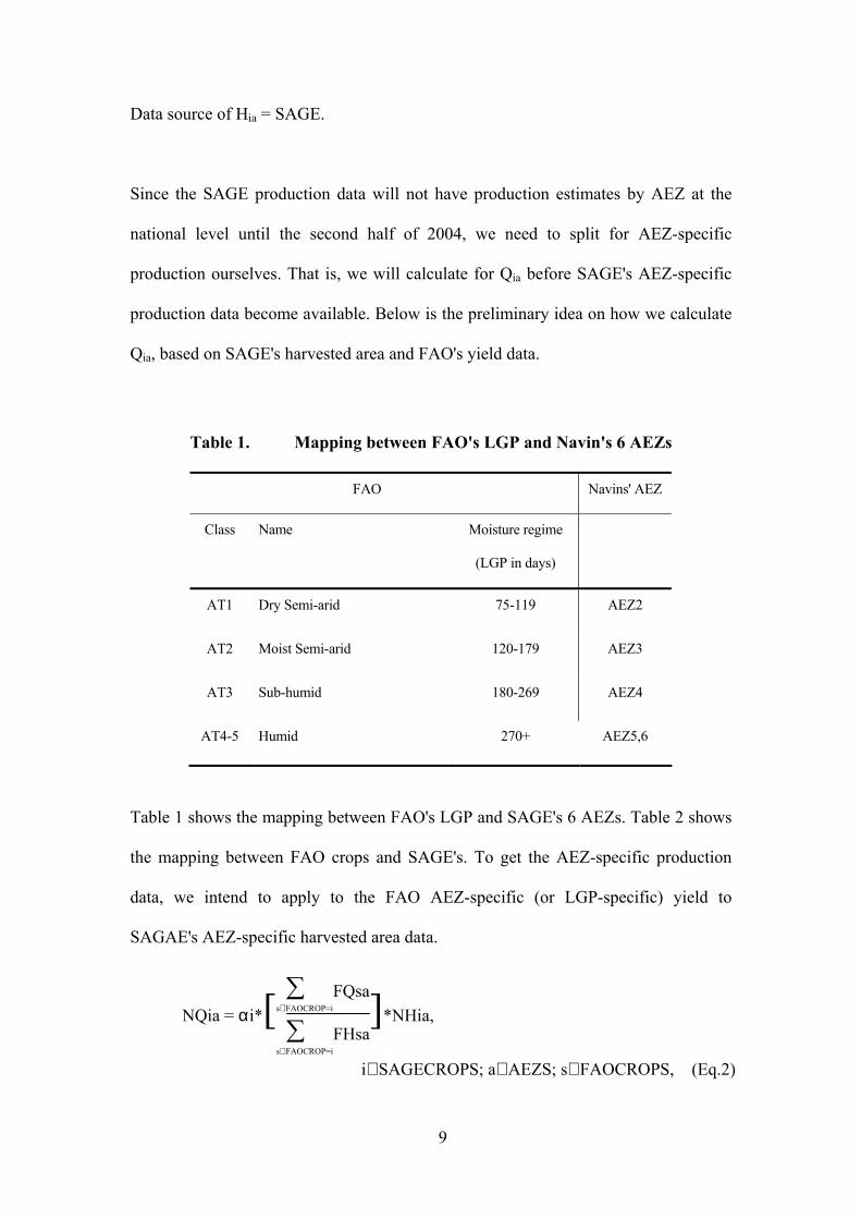
Data source of Hia = SAGE.
Since the SAGE production data will not have production estimates by AEZ at the
national level until the second half of 2004, we need to split for AEZ-specific
production ourselves. That is, we will calculate for Qia before SAGE's AEZ-specific
production data become available. Below is the preliminary idea on how we calculate
Qia, based on SAGE's harvested area and FAO's yield data.
Table 1. Mapping between FAO's LGP and Navin's 6 AEZs
FAO Navins' AEZ
Class Name Moisture regime
(LGP in days)
AT1 Dry Semi-arid 75-119 AEZ2
AT2 Moist Semi-arid 120-179 AEZ3
AT3 Sub-humid 180-269 AEZ4
AT4-5 Humid 270+ AEZ5,6
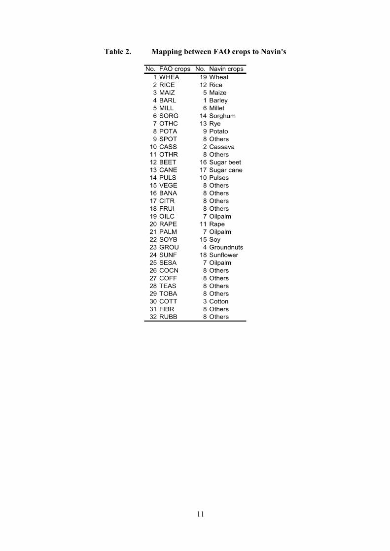
Table 1 shows the mapping between FAO's LGP and SAGE's 6 AEZs. Table 2 shows
the mapping between FAO crops and SAGE's. To get the AEZ-specific production
data, we intend to apply to the FAO AEZ-specific (or LGP-specific) yield to
SAGAE's AEZ-specific harvested area data.
NQia = αi*[ ∑s∈ FAOCROP=i
FQsa
∑s∈ FAOCROP=i
FHsa]*NHia,
i∈ SAGECROPS; a∈ AEZS; s∈ FAOCROPS, (Eq.2)
10
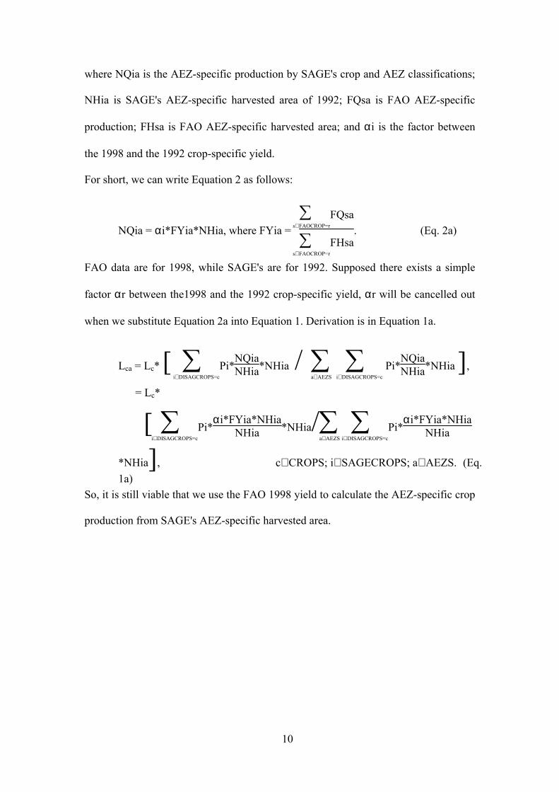
where NQia is the AEZ-specific production by SAGE's crop and AEZ classifications;
NHia is SAGE's AEZ-specific harvested area of 1992; FQsa is FAO AEZ-specific
production; FHsa is FAO AEZ-specific harvested area; and αi is the factor between
the 1998 and the 1992 crop-specific yield.
For short, we can write Equation 2 as follows:
NQia = αi*FYia*NHia, where FYia = ∑
s∈ FAOCROP=r
FQsa
∑s∈ FAOCROP=r
FHsa. (Eq. 2a)
FAO data are for 1998, while SAGE's are for 1992. Supposed there exists a simple
factor αr between the1998 and the 1992 crop-specific yield, αr will be cancelled out
when we substitute Equation 2a into Equation 1. Derivation is in Equation 1a.
Lca = Lc* [ ∑i∈ DISAGCROPS=c
Pi*NQiaNHia*NHia / ∑
a∈ AEZS
∑i∈ DISAGCROPS=c
Pi*NQiaNHia*NHia ],
= Lc*
[ ∑i∈ DISAGCROPS=c
Pi*αi*FYia*NHia
NHia *NHia/∑a∈ AEZS
∑i∈ DISAGCROPS=c
Pi*αi*FYia*NHia
NHia
*NHia], c∈ CROPS; i∈ SAGECROPS; a∈ AEZS. (Eq. 1a)
So, it is still viable that we use the FAO 1998 yield to calculate the AEZ-specific crop
production from SAGE's AEZ-specific harvested area.
11
Table 2. Mapping between FAO crops to Navin's
No. FAO crops No. Navin crops1 WHEA 19 Wheat2 RICE 12 Rice3 MAIZ 5 Maize4 BARL 1 Barley5 MILL 6 Millet6 SORG 14 Sorghum7 OTHC 13 Rye8 POTA 9 Potato9 SPOT 8 Others
10 CASS 2 Cassava11 OTHR 8 Others12 BEET 16 Sugar beet13 CANE 17 Sugar cane14 PULS 10 Pulses15 VEGE 8 Others16 BANA 8 Others17 CITR 8 Others18 FRUI 8 Others19 OILC 7 Oilpalm20 RAPE 11 Rape21 PALM 7 Oilpalm22 SOYB 15 Soy23 GROU 4 Groundnuts24 SUNF 18 Sunflower25 SESA 7 Oilpalm26 COCN 8 Others27 COFF 8 Others28 TEAS 8 Others29 TOBA 8 Others30 COTT 3 Cotton31 FIBR 8 Others32 RUBB 8 Others

12
Figure 2. The SAGE global map of the 18 AEZs
Table 3. Cropland distribution: China, 1992
C h in a croplan d (Un it: 1000h a)1 2 3 4 5 6 7 8
Paddy r ice W h eatC erea lgra in s
V egetables/fru its/n u ts O il seeds
Sugarcan e/beet
P lan t-basedfibres
C ropsN .E .C .
A E Z1 0 0 0 0 0 0 0 0A E Z2 0 0 0 0 0 0 0 0A E Z3 0 0 0 0 0 0 0 0A E Z4 18 5 10 2 2 2 0 10A E Z5 3699 69 367 284 547 497 1 2276A E Z6 145 1998 1100 207 546 134 695 538A E Z7 1418 6138 10340 1121 4956 587 457 5340A E Z8 1491 6180 9256 1161 3906 286 1011 7733A E Z9 1655 3707 5228 953 2760 242 452 3769A E Z10 6417 6920 3934 1223 3110 182 1118 10049A E Z11 28579 6314 6974 2753 7639 1654 884 19606A E Z12 93 1507 482 143 526 64 439 337A E Z13 88 971 237 77 415 15 13 266A E Z14 275 944 472 113 502 34 8 378A E Z15 256 404 227 54 131 15 10 330A E Z16 17 9 13 3 4 2 0 14A E Z17 0 0 0 0 0 0 0 0A E Z18 0 0 0 0 0 0 0 0T ota l 44149 35166 38639 8093 25044 3714 5086 50647

13
Table 4. Mapping of crops between SAGE and GTAP data
SAGE No. SAGE code GTAP No. GTAP code Description1 barley 3 gro Cereals grain n .e.c.2 cassava 4 v_f Vegetables, fruit, nuts3 cotton 7 pfb Plant-based fibres4 groundnuts 5 osd Oil seeds5 m aize 3 gro Cereals grain n .e.c.6 m illet 3 gro Cereals grain n .e.c.7 oilpalm 5 osd Oil seeds8 others 8 ocr Crops n .e.c.9 potato 4 v_f Vegetables, fruit, nuts
10 pulses 4 v_f Vegetables, fruit, nuts11 rape 5 osd Oil seeds12 rice 1 pdr Paddy rice13 rye 3 gro Cereals grain n .e.c.14 sorghum 3 gro Cereals grain n .e.c.15 soy 5 osd Oil seeds16 sugar beet 6 c_b Sugar cane, sugar beet17 sugar cane 6 c_b Sugar cane, sugar beet18 sunflower seeds 5 osd Oil seeds19 wheat 2 wht Wheat
Reference: Concordance, HS96 to GSC rev. 2: concordance between the 1996 edition of the Harm onized System and revision 2 of the GTAP sectoral classification.http://www.gtap.agecon.purdue.edu/resources/download/582.txt
Table 5. Mapping between FAO land classes (by LGP) and SAGE’s AEZs
FAO SAGE’s AEZ
Class Name Moisture regime (LGP in days)
AT1 Dry Semi-arid 75-119 AEZ2
AT2 Moist Semi-arid 120-179 AEZ3
AT3 Sub-humid 180-269 AEZ4
AT45 Humid 270+ AEZ5, 6
Proxies of AEZ-specific crop yields of countries not covered by FAO data
We run regression analysis to find out the relationship between yield of certain AEZ
(or AT) and the average yield of the country (all AEZs). Table 6 shows the regression
report of rice and wheat yields. Rice could not be grown in FAO land classes AT1 and
AT2, so there is zero yield. Rice yield in irrigated land is about 5 times of yield in
rainfed land class AT45. For wheat, rainfed land classes AT2 and AT3 are more
productive. For each crop (if the country is producing it), we apply the statistically

14
significant coefficients to the country average yield of the corresponding crop so as to
approximate AEZ-specific yield of the countries that are not covered in the FAO data.
We multiply this estimated AEZ-specific yield with SAGE's AEZ-specific harvested
area data to get the estimated AEZ-specific production. We later scale the estimated
AEZ-specific production to attain the country total production of the crop as shown in
the FAO data.
Table 6. Relationship of FAO land class specific yield against country
average yield: paddy rice and wheat
rice wheat AT1 v.s. country average 0.00 0.05 AT2 v.s. country average 0.00 0.21 AT3 v.s. country average 0.05 0.39 AT45 v.s. country average 0.24 0.14 AT67 v.s. country average 0.31 0.05 Irrigation v.s. country average 1.13 1.09
GTAP forest land rent data by 18 AEZs
The GTAP data base accounts land rent for agriculture land only. The forestry sector
does not incur agriculture land rent, but it does incur natural resource rent (see Section
18.C of Chapter 18 in Dimaranan and McDougall, 2002). We move the “natural
resource” rent to be the “land” rent for the forestry sector. We split the forestry land
rent into 18 AEZs according to the rental shares by AEZ. We derive the AEZ-specific
forestry land rent from Sohngen’s data of timberland rent by management type and
hectare by management type and by AEZ.

15
3. GTAP Greenhouse Gases Emissions Data
The GTAP greenhouse gases emissions data (Lee, 2002; 2003) account for the six
greenhouse gases as identified in the Kyoto Protocol. They are: (a) CO2, (b) CH4, (c)
N2O, and (d) F-gases, including HFC-134a, CF4, HFC-23, and SF6. We briefly
describe below how the GTAP greenhouse gases emissions data are compiled.
3.1 CO2
We follow the Tier 1 method as advised in the 1996 Revised IPCC guideline
(IPCC/OECD/IEA, 1997) to estimate CO2 emissions from fossil fuel combustion
based on the GTAP energy volume data of 1997, which is derived from the IEA
Energy Balances (OECE/IEA, 1999a; 1999b). We do not count emissions due to
feedstock use (i.e., natural gas and petroleum products used by the petrochemical
sector). We avoid double-counting of emissions from input use of coal, oil and gas by
the coal transformation, the petroleum refinery and the gas distribution sectors.
Emissions are accounted for use of coal products, petroleum products, and pipelined
or bottled gas.
3.2 Non-CO2 greenhouse gases
The CH4, N2O, and F-gases data are provided by the US Environmental Protection
Agency (US-EPA). The data from EPA identify various sources of emissions. We
further mapped the sources of emissions to GTAP sectors according to activities.
Tables 7 to 9 show the mapping between emission sources of CH4, N2O, and F-gases,
respectively, to GTAP sectors. Below we explain how we allocate each emission
source to the multiple pertinent GTAP sectors.

16
CH4 (see Table 7)
We allocate CH4 emissions from mobile sources to the household sector and the
transport sector of GTAP according to their consumption/output shares. We allocate
CH4 emissions from agriculture residue burning to the GTAP sectors coded as "PDR",
"WHT", "GRO", and "C_B", according to the output shares. We allocate CH4
emissions from enteric fermentation to the GTAP sectors of ruminants—i.e., "CTL"
and "RMK"—according to their shares of capital (as a proxy of herd size). We
allocate CH4 emissions from manure management to the GTAP livestock sectors—i.e.,
"CTL", "OAP" and "RMK"—according to their shares of capital (as a proxy of herd
size).
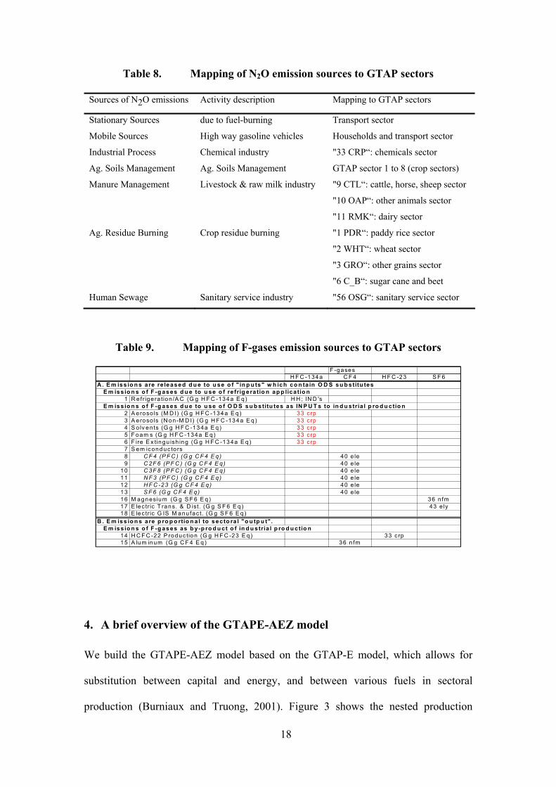
N2O (see Table 8)
We allocate N2O emissions from mobile sources to the household sector and the
transport sector of GTAP according to their consumption/output shares. We allocate
N2O emissions from agriculture soil management (mainly due to fertilizer use) to the
GTAP crop sectors—i.e., "PDR", "WHT", "GRO", "V_F", "OSD", "C_B", "PFB",
and "OCR"—according to the output shares. We allocate N2O emissions from manure
management to the GTAP livestock sectors— i.e., "CTL", "OAP" and "RMK"—
according to their shares of capital (as a proxy of herd size). We allocate N2O
emissions from agriculture residue burning to the GTAP sectors coded as "PDR",
"WHT", "GRO", and "C_B", according to the output shares.
17
F-gases (see Table 9)
We allocate HFC-134a emissions from refrigerator and air conditioning to the
household sector and all the manufacture and service sectors of GTAP according to
their consumption/output shares.
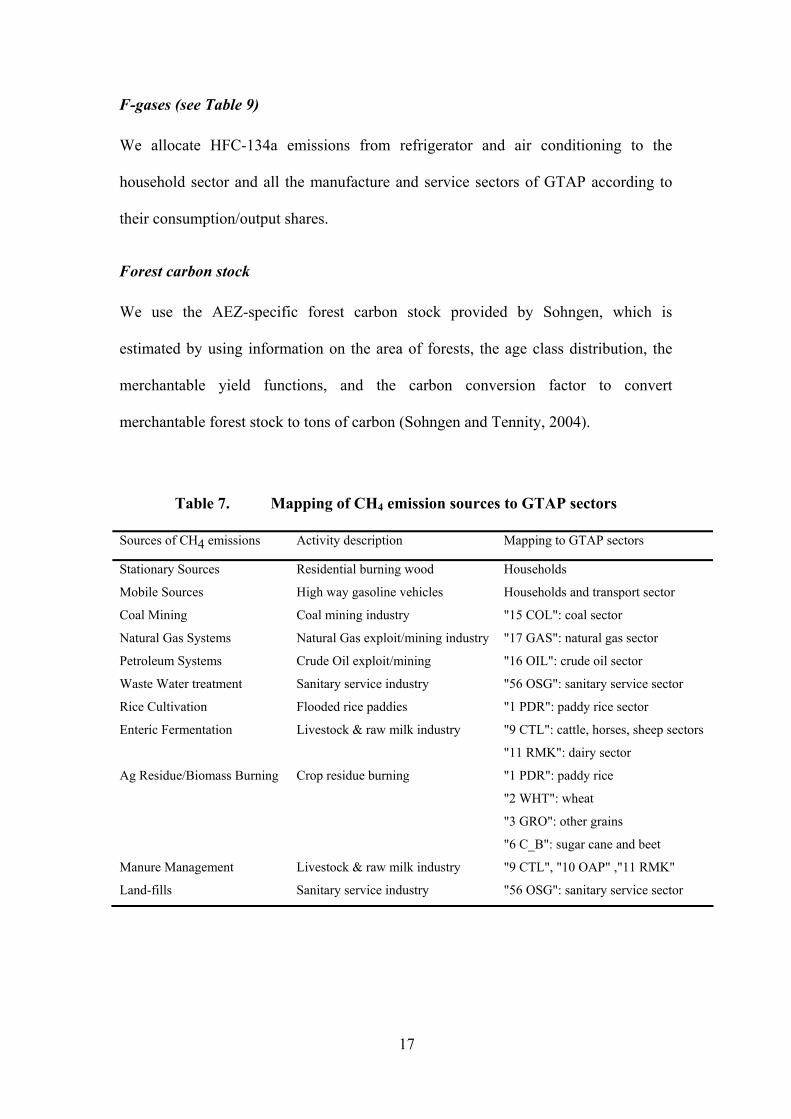
Forest carbon stock
We use the AEZ-specific forest carbon stock provided by Sohngen, which is
estimated by using information on the area of forests, the age class distribution, the
merchantable yield functions, and the carbon conversion factor to convert
merchantable forest stock to tons of carbon (Sohngen and Tennity, 2004).
Table 7. Mapping of CH4 emission sources to GTAP sectors
Sources of CH4 emissions Activity description Mapping to GTAP sectors
Stationary Sources Residential burning wood Households
Mobile Sources High way gasoline vehicles Households and transport sector
Coal Mining Coal mining industry "15 COL": coal sector
Natural Gas Systems Natural Gas exploit/mining industry "17 GAS": natural gas sector
Petroleum Systems Crude Oil exploit/mining "16 OIL": crude oil sector
Waste Water treatment Sanitary service industry "56 OSG": sanitary service sector
Rice Cultivation Flooded rice paddies "1 PDR": paddy rice sector
Enteric Fermentation Livestock & raw milk industry "9 CTL": cattle, horses, sheep sectors
"11 RMK": dairy sector
Ag Residue/Biomass Burning Crop residue burning "1 PDR": paddy rice
"2 WHT": wheat
"3 GRO": other grains
"6 C_B": sugar cane and beet
Manure Management Livestock & raw milk industry "9 CTL", "10 OAP" ,"11 RMK"
Land-fills Sanitary service industry "56 OSG": sanitary service sector
18
Table 8. Mapping of N2O emission sources to GTAP sectors
Sources of N2O emissions Activity description Mapping to GTAP sectors
Stationary Sources due to fuel-burning Transport sector
Mobile Sources High way gasoline vehicles Households and transport sector
Industrial Process Chemical industry "33 CRP“: chemicals sector
Ag. Soils Management Ag. Soils Management GTAP sector 1 to 8 (crop sectors)
Manure Management Livestock & raw milk industry "9 CTL“: cattle, horse, sheep sector
"10 OAP“: other animals sector
"11 RMK“: dairy sector
Ag. Residue Burning Crop residue burning "1 PDR“: paddy rice sector
"2 WHT“: wheat sector
"3 GRO“: other grains sector
"6 C_B“: sugar cane and beet
Human Sewage Sanitary service industry "56 OSG“: sanitary service sector
Table 9. Mapping of F-gases emission sources to GTAP sectors
F -gasesH F C -134a C F 4 H F C -23 S F 6
A . E m iss io n s are re leased d u e to u se o f " in p u ts" w h ich co n ta in O D S su b stitu tesE m issio n s o f F -g ases d u e to u se o f re frig era tio n ap p lica tio n
1 R e frige ra tion /A C (G g H F C -134a E q) H H ; IN D 'sE m issio n s o f F -g ases d u e to u se o f O D S su b stitu tes as IN P U T s to in d u stria l p ro d u ctio n
2 A eroso ls (M D I) (G g H F C -134a E q ) 33 c rp3 A eroso ls (N on -M D I) (G g H F C -134a E q ) 33 c rp4 S o lv en ts (G g H F C -134a E q ) 33 c rp5 F oam s (G g H F C -134a E q ) 33 c rp6 F ire E x tingu ish ing (G g H F C -134a E q ) 33 c rp7 S em iconduc to rs8 C F 4 (P F C ) (G g C F 4 E q ) 40 e le9 C 2F 6 (P F C ) (G g C F 4 E q) 40 e le
10 C 3F 8 (P F C ) (G g C F 4 E q) 40 e le11 N F 3 (P F C ) (G g C F 4 E q ) 40 e le12 H F C -23 (G g C F 4 E q ) 40 e le13 S F 6 (G g C F 4 E q ) 40 e le16 M agnesium (G g S F 6 E q ) 36 n fm17 E lec tric T rans. & D ist. (G g S F 6 E q ) 43 e ly18 E lec tric G IS M anu fac t. (G g S F 6 E q )
B . E m iss io n s are p ro p o rtio n a l to sec to ra l "o u tp u t" .E m iss io n s o f F -g ases as b y -p ro d u ct o f in d u stria l p ro d u ctio n
14 H C F C -22 P roduc tion (G g H F C -23 E q ) 33 c rp15 A lum inum (G g C F 4 E q ) 36 n fm
4. A brief overview of the GTAPE-AEZ model
We build the GTAPE-AEZ model based on the GTAP-E model, which allows for
substitution between capital and energy, and between various fuels in sectoral
production (Burniaux and Truong, 2001). Figure 3 shows the nested production

19
structure in the GTAP-E model. Sectors may substitute energy for capital when
energy price rises more than capital rental does. The inter-fuel substitution comprises
of three sub-nestings: (a) electricity v.s. non-electricity composite; (b) coal v.s. non-
coal composite; and (c) between oil, gas, and petroleum products. For example,
sectors may substitute coal for non-coal fuel (a composite of oil, gas and petroleum
products) when coal is more expensive than non-coal fuels.
In the GTAPE-AEZ model, we recognize a unique production function for each of
the land-using sectors located in a specific AEZ. For example, the paddy rice sector
located in AEZ 1 has a different production function from the paddy rice sector
located in AEZ 6. This is to identify the difference in the productivity of land of
different climate characteristics. Nevertheless, all the paddy rice sectors located in the
six AEZs produce homogenous output to meet market demand.
We assume that transition of land in a specific AEZ can occur only between
sectors that the land is appropriate for their use. This is a new concept beyond the
standard GTAP model, in which land is assumed to be transformable between uses of
crop growing, livestock breeding, or timber plantation, regardless of climatic or soil
constraints. Facts show that most crops can only grow on lands that is under certain
temperature, moisture, soil type, land form, etc.. We believe that the introduction of
the agro-ecological zoning (AEZ) renders a sound presentation of sectoral
competition for land.
In GTAPE-AEZ, we associate methane (CH4) and nitrous oxide (N2O) emissions
to their emitting sources (or drivers). For example, we link methane emissions from
paddy rice cultivation to the land used in the paddy rice sector. Following the
approach of Hyman (2001), we treat methane emissions as input to the paddy rice
20
growing, and permit limited substitution of other input for emissions according to
estimates of the marginal cost of abatement.
Figure 4 shows the production structure of the paddy rice sector located in AEZ 2.
This paddy rice sector (“PDR_AEZ2”) uses land in AEZ 2 only, but no land from
other AEZs. The paddy rice sector located in AEZ uses only land in AEZ 2. We
associate CH4 emissions with the land acreage of rice paddies, and assume CH4
emissions are proportional to area harvested. We associate N2O emissions to fertilizer
use by the paddy rice sector and again assume fixed proportion between N2O
emissions and fertilizer use.
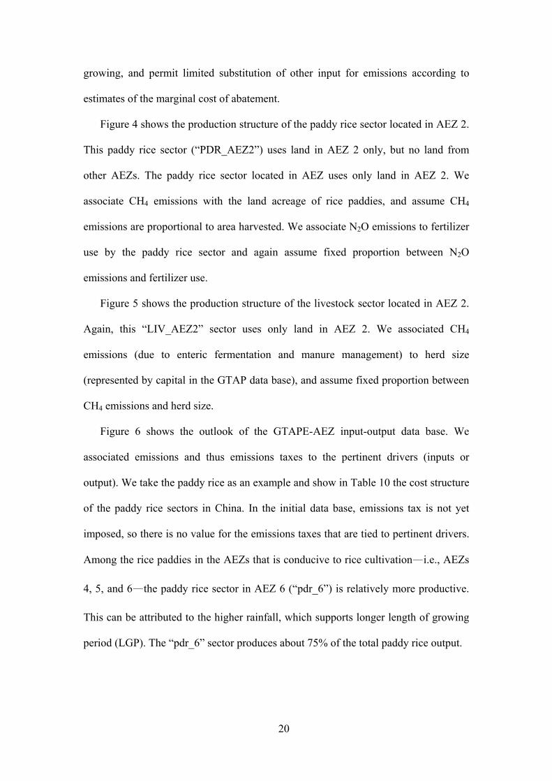
Figure 5 shows the production structure of the livestock sector located in AEZ 2.
Again, this “LIV_AEZ2” sector uses only land in AEZ 2. We associated CH4
emissions (due to enteric fermentation and manure management) to herd size
(represented by capital in the GTAP data base), and assume fixed proportion between
CH4 emissions and herd size.
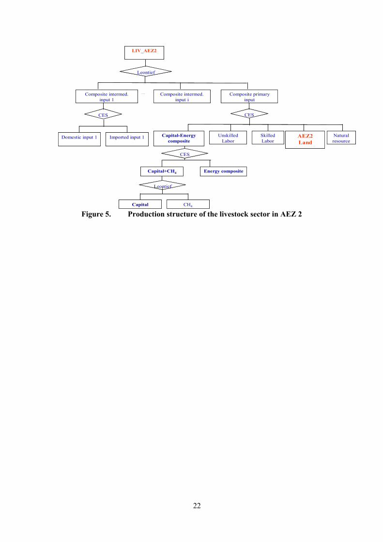
Figure 6 shows the outlook of the GTAPE-AEZ input-output data base. We
associated emissions and thus emissions taxes to the pertinent drivers (inputs or
output). We take the paddy rice as an example and show in Table 10 the cost structure
of the paddy rice sectors in China. In the initial data base, emissions tax is not yet
imposed, so there is no value for the emissions taxes that are tied to pertinent drivers.
Among the rice paddies in the AEZs that is conducive to rice cultivation—i.e., AEZs
4, 5, and 6—the paddy rice sector in AEZ 6 (“pdr_6”) is relatively more productive.
This can be attributed to the higher rainfall, which supports longer length of growing
period (LGP). The “pdr_6” sector produces about 75% of the total paddy rice output.

21
Output
Primary factors Intermediate goods(non-energy)
Skilled Lab.
Nat. Resource
Land
GasOil Petroleum prods
EnergyCapital
Electricity
K-E composite
Non-Coal
Non-Electricity
Coal
Unskilled Lab.
Output
Primary factors Intermediate goods(non-energy)
Skilled Lab.
Nat. Resource
Land
GasOil Petroleum prods
EnergyCapital
Electricity
K-E composite
Non-Coal
Non-Electricity
Coal
Unskilled Lab.
Figure 3. Production structure in GTAP-E
Leontief
Composite intermed. input 1
Composite intermed. input i
…. Composite primary input
CES
AEZ2Land +
CH4
Skilled Labor
Natural resource
Unskilled Labor
Capital-Energy
composite
PDR_AEZ2
Leontief
AEZ2 Land CH4
Fertilizer+N2O
Leontief
Fertilizer N2O
Leontief
Composite intermed. input 1
Composite intermed. input i
…. Composite primary input
CES
AEZ2Land +
CH4
Skilled Labor
Natural resource
Unskilled Labor
Capital-Energy
composite
PDR_AEZ2
Leontief
AEZ2 Land CH4
Fertilizer+N2O
Leontief
Fertilizer N2O
Figure 4. Production structure of the paddy rice sector in AEZ 2
22
Leontief
Composite intermed. input 1
Composite intermed. input i
…. Composite primary input
CES
AEZ2Land
Skilled Labor
Natural resource
Unskilled Labor
Capital-Energy composite
CES
Domestic input 1 Imported input 1
LIV_AEZ2
Leontief
Capital CH4
CES
Capital+CH4 Energy composite
Leontief
Composite intermed. input 1
Composite intermed. input i
…. Composite primary input
CES
AEZ2Land
Skilled Labor
Natural resource
Unskilled Labor
Capital-Energy composite
CES
Domestic input 1 Imported input 1
LIV_AEZ2
Leontief
Capital CH4
CES
Capital+CH4 Energy composite
Figure 5. Production structure of the livestock sector in AEZ 2
23
Absorption Matrix
1 2 3 4 5 6
Producers Investors Household Export Government Int'l transport Total
Sizes 1 1 1 1 1 1
Comm. Flows
Emissions tax
on inputs N/A
Land 6
Emissions tax
on land 6
Tax/Subsidy on
C sequestration 6
Natural
Resources 1
Labour 2
Capital 1
Emissions tax
on output 1
Total Costs 1
Production
Taxes 1
Figure 6. Outlook of the GTAPE-AEZ data base

24
Table 10. Cost structure: paddy rice, China
China_PDR pdr_1 pdr_2 pdr_3 pdr_4 pdr_5 pdr_6 Total
Int’med. Inputs 0 0 0 936.3 1114.4 5575.8 7626.5
Land_pdr_1 0 0 0 0 0 0 0
Land_pdr_2 0 0 0 0 0 0 0
Land_pdr_3 0 0 0 0 0 0 0
Land_pdr_4 0 0 0 227.0 0 0 227.0
Land_pdr_5 0 0 0 0 621.1 0 621.1
Land_pdr_6 0 0 0 0 0 3435.2 3435.2
Unskilled Labor 0 0 0 1061.3 1263.1 6320.2 8644.6
Skilled Labor 0 0 0 8.6 10.2 51 69.7
Capital 0 0 0 217.6 259 1295.8 1772.4
Natural Resource 0 0 0 0 0 0 0
Total 0 0 0 2450.8 3267.8 16678.0 22396.5
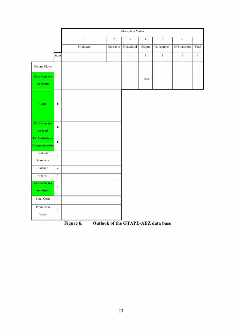
5. An Illustrative Simulations
We run the GTAPE-AEZ model with an aggregated data base of three regions (i.e.,
the U.S., China, and rest of world), 23 commodities and 48 sectors (=5*6 + 18; each
of the first five land-based sectors are further disaggregated into 6 AEZ-specific sub-
sectors). Table 11 shows the sectoral aggregation scheme of the GTAP data base for
the prototype GTAPE-AEZ model.
25
Table 11. Sectoral aggregation scheme of the prototype GTAPE-AEZ model
No. New sector code Sector description Comprising old sectors:
1 PaddyRice Paddy Rice pdr
2 WheatGrains Wheat and Grains wht gro
3 Livestock Livestock ctl oap rmk
4 OthAg Other Ag Production v_f osd c_b pfb ocr
5 Forestry Forestry (timber) for
6 OthPrimInd Other Primary Ind Production wol fsh omn
7 Coal Coal col
8 Oil Oil oil
9 Gas Gas gas
10 CSGHMeat Ruminant Meat cmt
11 OthMeat Other Meat omt
12 OthFoodProd Other Food Products vol sgr ofd b_t
13 DairyProd Dairy Products mil
14 ProcsdRice Processed Rice pcr
15 OthManufact Other Manufacture tex wap lea fmp mvh otn ele ome omf wtr
16 WoodProd Wood Products lum
17 PaperProd Paper Products ppp
18 PetrolumProd Petroleum Products p_c
19 EI_Manufact Energy Intensive Manufacture crp nmm i_s nfm
20 Electricity Electricity ely
21 GasDistrib Gas Distribution gdt
22 Construction Construction cns
23 Service Service trd otp wtp atp cmn ofi isr obs ros osg dwe
We first run a set of simulations of various scenarios—abating CO2 only v.s.
multiple gases, coupled with various degrees of land mobility—and develop aggregate
marginal abatement cost curve for each country. This is described in section 5.1. In
section 5.2, we look at some selective sectoral results of a 10% reduction of all gases.
26
5.1 Marginal abatement cost curves
We run four experiments and develop aggregate marginal abatement cost curve for
each country under the no emission trading scenario. In experiment (a), only CO2
emissions from fossil fuel combustion are reduced, and forest carbon is not included.
In experiments (b), (c), and (d), all greenhouse gases, plus forest carbon, are included
in the abatement basket. We specify no land mobility between uses in experiment (b).
We specify -1.0 and -5.0 of CET transformation elasticities of land between uses in
experiments (c) and (d), respectively.
Figures 7 and 8 show the aggregate marginal abatement cost curves of the U.S.
and China, respectively, under the four sets of scenarios. In the CO2 only case, the
marginal abatement cost curve (MAC) of the U.S. (Figure 7) is in line with the U.S.
MACs as seen in the literature—for example, Ellerman and Decaux (1998), and other
estimates by the EMF study as reported in IPCC (2001)—although a little bit lower.
This is mainly because GTAPE-AEZ is currently a comparative static model, while
the other MAC estimates are obtained from the dynamic model for the 2010 reduction
target. Emissions abatement by 2010 is more costly than by 1997 due to economic
growth, supposing that there is no dramatic improvement in clean development
technology.
Comparing the MACs of experiments (a) and (b)—i.e., the CO2 only v.s. the
multi-gas with zero land mobility—we see that the marginal cost of multiple gases
abatement is lower that that of the CO2-only case, as there is efficiency gain in the
multi-gas abatement. Initial abatement of non-CO2 gases is normally cheaper. This
also conforms with the results as other global CGE models estimate, e.g., Burniaux
(2000), Reilly et al. (1999), Reilly, Mayer, and Harnisch (2000), Kets (2002), and
Brown et al. (1999). Comparing the MACs of experiments (b), (c), and (d)—the

27
easier mobility of land among uses further helps reduce the abatement cost: about
30% lower when the land mobility parameter (CET elasticity) is -1.0, relatively to the
zero land mobility; and about 70% lower when the CET elasticity is extremely large (-
5.0).
USA MACC
0
20
40
60
80
100
120
140
160
-1% -5% -10% -15% -20% -30% -40%
Abatement %
1997
US
$/to
n C co2 only
all gases +sig=0
all gases +sig=1.0
all gases +sig=5
Figure 7. Marginal abatement cost curve of the U.S.

28
China MACC
0
5
10
15
20
25
30
35
40
1 2 3 4 5 6 7
abatement
1997
US
$/to
n C co2 only
all gases +sig=0
all gases +sig=1.0
all gases +sig=5
Figure 8. Mapping of CH4 emission sources to GTAP sectors
5.2 Land transitions between uses under a 10% reduction of all GHGs
Table 12 shows the land transition between the land-based sectors of China. Most of
the land-based sectors are reducing its land acreage, and the shifted land is absorbed
by the forestry sector (“FOR”). To reduce land-based GHG emissions, a tax is
imposed, and this tax raises the cost of, for example, rice production. The paddy rice
sectors of all AEZs are subject to this tax. So, the supply curve of paddy rice shifts up,
and thus the price goes up, which discourages demand. In turn, the decline in demand
for paddy rice drives down the equilibrium price of paddy rice. The prices of other
inputs also rise due to the carbon tax. Revenue is squeezed by the increase in input
costs. Thus, land rent declines.
One the other hand, the forest sector is assumed to be able to absorb carbon. In
GTAPE-AEZ, we assume that forest carbon stock is proportional to land acreage. The
forestry sector is subsidized due to its credit in carbon absorption. The supply curve of

29
the forestry sector shifts outwards due to the subsidy. The increase in revenue boosts
land rent of forestry. Within the same AEZ, land therefore flows to the forestry sector.
When we examine the sectoral land use results, we find that the AEZs where the
crop is mostly grown are suffering most. For example, the rice paddy acreage of
higher rainfall AEZs (e.g., AEZs 5 and 6) reduces more, compared to rice paddies in
other AEZs. Note that we assume paddy rice sectors located in all AEZs are
producing homogeneous product. The market price of paddy rice falls as a
consequence of the carbon tax. All the paddy rice sectors (in the 6 AEZs) face the
same market price. The higher rainfall AEZs—that are more productive and thus incur
higher land rent—bear more of the revenue-cost squeeze. Furthermore, the higher
rainfall AEZs of the paddy rice sector are relatively more CH4-intensive. So we see
more decline in land acreage of higher rainfall AEZs. The Other Crop sector (“OAG”)
also has similar context as the paddy rice sector. The Wheat sector (“WHT”) is most
located in AEZs 2 and 3. So its AEZs 2 and 3 acreage shrinks more than other AEZs.
As all land-based sectors are losing land, the forestry sector is gaining land, and
thus absorbs more carbon (-8.24%). Table 13 shows the AEZ-specific contributions of
the increase in forest land to its carbon absorption. Most of the contribution comes
from AEZ 6 (6.26% out of 8.24% in magnitude). The paddy rice sector (“PDR”) and
the Other Crop sector (“OAG”) are the key source of land supply to the forest sector.
30
Table 12. Land transition between sectors: China
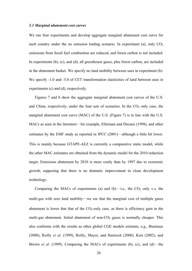
China PDR WHT LIV OAG FOR
Land_AEZ1(%) 0 -1.35 -1.8 -1.6 1.02
Land_AEZ2(%) 0 -3.0 -1.9 -1.8 2.35
Land_AEZ3(%) 0 -3.0 -2.4 -3.8 2.65
Land_AEZ4(%) -1.8 -2.2 -1.8 -2.8 2.50
Land_AEZ5(%) -2.6 -2.0 -1.5 -3.9 2.62
Land_AEZ6(%) -2.9 -2.5 -2.0 -10.2 9.42
GHG emissions (%) -2.3 -2.7 -2.1 -7.7 -8.24
Table 13. Contributions of land use change to greenhouse gases
sequestration in forest: China
China Contribution to GHG emissions
Land_AEZ1(%) -0.00
Land_AEZ2(%) -0.25
Land_AEZ3(%) -0.86
Land_AEZ4(%) -0.57
Land_AEZ5(%) -0.39
Land_AEZ6(%) -6.26
GHG emissions (%) -8.24
6. Concluding remarks and future research agenda
The paper describes the on-going project of the GTAP land use data base. We also
present the GTAPE-AEZ model, which illustrates how land use and land-based
emissions can be incorporated in the CGE framework for Integrated Assessment (IA)
of climate change policies. We follow the FAO fashion of agro-ecological zoning
(FAO, 2000; Fischer et al, 2002) to identify lands located in six zones. Lands located
in a specific AEZ have similar (or homogenous) soil, landform and climatic
characteristics. The six AEZs range over a spectrum of length of growing period

31
(LGP) for which their climate characteristics can support for crop growing. AEZ 1
covers the land of the temperature and moisture regime that is able to support length
of growing period (LGP) up to 60 days per annum. On the other end of the LGP
spectrum, lands in AEZ 6 can support a LGP from 270 to 360 days per annum. Crop
growing, livestock breeding, and timber plantation are dispersed on lands of each
AEZ of the six, whichever meets their climatic and edaphic requirements.
In GTAPE-AEZ, we assume that land located in a specific AEZ can be moved
only between sectors that the land is appropriate for their use. That is, land is mobile
between crop, livestock and forestry sectors within, but not across, AEZ’s. In the
standard GTAP model, land is assumed to be transformable between uses of crop
growing, livestock breeding, or timber plantation, regardless of climatic or soil
constraints. The fact is that most crops can only grow on lands that is under certain
temperature, moisture, soil type, land form, etc.. The same concern arises for land use
by the livestock and the forestry sectors. Lands that are suitable for growing wheat
may not be good for rice cultivation alike, even under transformation at a reasonable
cost. The introduction of the agro-ecological zoning in GTAP helps to clear up the
counterfactual assumption in inter-sectoral land transition, and permit a sound
presentation of sectoral competition for land.
In GTAP-AEZ, we recognize a unique production function for each of the land-
using sectors located in a specific AEZ. For example, the paddy rice sector located in
AEZ 1 has a different production function from the paddy rice sector located in AEZ
6. This is to identify the difference in the productivity of land of different climate
characteristics. Nevertheless, all the paddy rice sectors located in the six AEZs
produce homogenous output to meet market demand.
32
In GTAP-AEZ, we associate methane (CH4) and nitrous oxide (N2O) emissions to
their emitting sources (or drivers). For example, we link methane emissions from
paddy rice cultivation to the land used in the paddy rice sector of GTAP-AEZ. We
treat methane emissions as input to the paddy rice growing, and permit limited
substitution of other input for emissions according to estimates of the marginal cost of
abatement, following the approach of Hyman (2001).
For future research, we plan to address the dynamics of forest carbon
sequestration, which is closely related to forest growth and harvest. Biomass growth is
a key factor to forest carbon stock. Biomass growth varies by age of trees and by
management intensity of timberland. This in turn affects the forest carbon
sequestration potential. On the other hand, timber harvest causes carbon emissions.
These features of forest and carbon sequestration need to be tackled in a dynamic
framework.
References:
Brown, S., Kennedy, D., Polidano, D., Woffenden, K., Jakeman, G., Graham, G.,
Jotzo, F., And Fisher, B. (1999). Economic Impacts of the Kyoto Protocol:
Accounting for the Three Major Greenhouse Gases, Australian Bureau of
Agricultural and Resource Economics (ABARE), Research Report 99.6, Canberra,
Australia.
Burniaux, J.-M. (2000). A Multi-Gas Assessment of the Kyoto Protocol, OECD
(ECO/WKP-2000-43).
Burniaux, J.-M., and Truong, T. (2001). GTAP-E: An Energy-Environmental Version
of the GTAP Model. GTAP Technical Paper No. 16. Center for Global Trade

33
Analysis, Purdue University, West Lafayette, IN 47907, U.S.A. Available at
http://www.gtap.agecon.purdue.edu/resources/res_display.asp?RecordID=923.
Dimarana, B. V., and McDougall, R. A. (2002). Global Trade, Assistance, and
Production: the GTAP 5 Data Base. Center for Global Trade Analysis, Purdue
University, West Lafayette, IN 47907, U.S.A.
Ellerman, A.D., and A. Decaux. (1998). Analysis of Post-Kyoto CO2 Emissions
Trading Using Marginal Abatement Curves. MIT Joint Program on the Science
and Policy of Global Change, Report No. 40, Massachusetts Institute of
Technology (MIT).
EMF. (2003). EMF 21: Multi-Gas Mitigation and Climate Change. The Energy
Modeling Forum (EMF), Stanford University, Palo Alto, CA. Available:
http://www.stanford.edu/group/EMF/research/index.htm.
FAO. (2000). Land Cover Classification System: Classification Concepts and User
Manual (with CD-Rom). Rome: Food and Agriculture Organization (FAO) of the
United Nations.
FAO and IIASA. (2000). Global Agro-Ecological Zones - 2000. Food and Agriculture
Organization (FAO) of the United Nations, Rome, Italy, and International Institute
for Applied Systems Analysis (IIASA), Laxenburg, Austria.
Fischer, G., van Velthuizen, H., Shah, M., and Nachtergaele, F. (2002). Global Agro-
Ecological Assessment for Agriculture in the 21st Century: Methodology and
Results (Research Report RR-02-02). Laxenburg, Austria: International Institute
for Applied Systems Analysis (IIASA) and Food and Agriculture Organization
(FAO) of the United Nations (UN).
GTAP Website. (2002). Workshop: Incorporation of Land Use and Greenhouse Gas
Emissions into the GTAP Data Base. Center for Global Trade Analysis (GTAP),

34
Purdue University, West Lafayette, IN 47907, U.S.A. Available:
http://www.gtap.agecon.purdue.edu/databases/projects/Land_Use_GHG/MIT_Wo
rkshop/default.asp.
Hertel, T. W. (eds.). (1997). Global Trade Analysis: Modeling and Applications.
Cambridge University Press.
Hyman, R. C. (2001). A More Cost-Effective Strategy for Reducing Greenhouse Gas
Emissions: Modeling the Impact of Methane Abatement Opportunities.
Unpublished Master thesis, Massachusetts Institute of Technology, Cambridge,
Massachusetts.
IPCC. (2001). Climate Change 2001: Mitigation. Contribution of Working Group III
to the Third Assessment Report (TAR) of the Intergovernmental Panel on Climate
Change (IPCC). B. Metz, O. Davidson, R. Swart, and J. Pan (eds.). Cambridge
University Press, U.K. 700 pp.
IPCC/OECD/IEA. (1997). Revised 1996 IPCC Guidelines for National Greenhouse
Gas Inventories. Paris: Intergovernmental Panel on Climate Change (IPCC),
Organization for Economic Co-operation and Development (OECD), International
Energy Agency (IEA).
Kets, W. (2002), Scope for Non-CO2 Greenhouse Gases in Climate Policy, CPB
Report 2002/1.
Lee, H.-L. (2002). An Emissions Data Base for Integrated Assessment of Climate
Change Policy Using GTAP. Center for Global Trade Analysis (GTAP), Purdue
University, West Lafayette, IN 47907, U.S.A. Available:
http://www.gtap.agecon.purdue.edu/resources/res_display.asp?RecordID=1143.

35
Lee, H.-L. (2003). The GTAP Non-CO2 Emissions Data. Center for Global Trade
Analysis (GTAP), Purdue University, West Lafayette, IN 47907, U.S.A. Available:
http://www.gtap.agecon.purdue.edu/resources/res_display.asp?RecordID=1186.
OECD/IEA. (1999a). Energy Balances of OECD Countries, 1996-1997. Paris:
Organization for Economic Co-operation and Development (OECD), International
Energy Agency (IEA).
OECD/IEA. (1999b). Energy Balances of Non-OECD Countries, 1996-1997. Paris:
Organization for Economic Co-operation and Development (OECD), International
Energy Agency (IEA).
Reilly, J., Prinn, R., Harnisch, J., Fitzmaurice, J., Jacoby, H., Kicklighter, D., Melillo,
J., Stone, P., Sokolov, A., Wang, C. (1999). Multi-gas Assessment of the Kyoto
Protocol, Nature, Vol. 401, 7 October 1999 (pp. 549-55).
Reilly, J., Mayer, M., and Harnisch, J. (2000). Multiple Gas Control under the Kyoto
Agreement, MIT Joint Program on the Science and Policy of Global Change,
Report no. 58.
Sohngen, B., and Tennity, C. (2004). Country Specific Global Forest Data Set V.1.
memo. Department of Agricultural, Environmental, and Development Economics,
Ohio State University, Columbus, OH 43210, U.S.A.