Income Prediction Errors: Sources and Implications for Physician Behavior

Sean Nicholson Cornell University and NBER

133 MVR Hall Ithaca, NY 14853

sn243@cornell.edu ph: (607) 254-6498 fax: (607) 255-4071

Nicholas S. Souleles The Wharton School

University of Pennsylvania and NBER

March 2005

Abstract Although income expectations play a central role in many economic decisions, little is known about the sources of income prediction errors and how people respond to income shocks. This paper uses a unique panel data set to examine the accuracy of physicians’ income expectations, the sources of income prediction errors, and the effect of income prediction errors on physician behavior. The data set contains direct survey measures of income expectations for a generation of medical students, their corresponding income realizations, and a rich summary of the shocks hitting their medical practices. We find that income prediction errors were positive on average over the sample period, but varied significantly over time and cross-sectionally. We trace these results to aggregate and group-level shocks, especially persistent specialty-specific shocks such as the growth of HMOs and other changes in the health care market. Physicians who experienced negative income shocks were more likely to respond by increasing their hours worked. JEL codes: J24; J3; J44; I11; D84 Key words: physician income, income expectations; income prediction errors; rational expectations.

1 I. Introduction

Income expectations are an important determinant of many economic decisions, including

schooling and occupational choice. However, little is known about the accuracy of income expectations,

the sources of income prediction errors, and how people respond to income shocks (Manski, 1993). Since

income expectations are rarely directly observed, the most common approach in empirical applications is to

assume that expectations are rational and infer income expectations from panel data on realized income.

(See Dominitz and Manski (1997) for a review of this literature, and Willis and Rosen (1979) for an

example of this approach.) However, Manski (1993) has shown that misspecifying how income

expectations are formed can lead to incorrect inferences about peoples’ behavior given their expectations,

for instance the responsiveness of school enrollment to the expected return to schooling.

There are only a few existing studies that assess the accuracy of income expectations, usually by

comparing survey measures of income expectations with subsequent income realizations. Das and van

Soest (1999) examine data from the Dutch Socio-Economic Panel, which asked people to predict whether

in the next year their household income would decrease, remain unchanged, or increase. They find that

between 1984 and 1989 their sample substantially underestimated their income growth; i.e., income

expectations were too pessimistic on average. Using a U.S. sample, Dominitz (1998) compares one-year-

ahead income predictions in 1993, elicited in the form of (continuous) subjective probabilities, with

peoples’ actual income in 1994. He finds income expectations were too optimistic, by contrast.1

There are a number of limitations to the existing literature. First, one should not necessarily

1 Most other studies of the accuracy of household expectations have used aggregated data on inflation

expectations (e.g., Maddala, Fishe, and Lahiri, 1981; Gramlich, 1983; Batchelor, 1986). However, when agents’ information sets differ, aggregation can lead to spurious rejections of rationality. Some papers have modeled occupational choice without directly observing peoples’ subjective income expectations. Zarkin (1985) examines whether prospective teachers incorporate forecastable future demand conditions into their decision to enter the occupation. He finds that future student enrollment rationally affects the occupational decisions of secondary school teachers, but not of elementary school teachers. Siow (1984) assumes that prospective lawyers expect future cohorts of students to arbitrage away any rents that would otherwise occur from a wage shock. He finds evidence consistent with his model.

2 expect prediction errors to average out to zero over a relatively short sample period (Souleles, 2003; Keane

and Runkle, 1998). As a result, expectations that are rational ex ante might not appear rational ex post.

For instance, the respondents in the two studies above might by chance have received positive and negative

income shocks, respectively, on average over their relatively short sample periods. Analyses of the

accuracy of income expectations therefore require long sample periods. Souleles (2003) examines 18 years

of monthly data from the Michigan Survey of Consumer Attitudes and Behavior. This survey records

household expectations and subsequent realizations for a number of variables, including household income

and financial security, inflation, and aggregate economic activity. Souleles finds that even over a long

sample period, expectations of most of these variables appear to have been biased and inefficient, at least

ex post. He traces these results in part to aggregate shocks, like the business cycle and changes in

monetary policy regime, as well as group-level shocks (e.g., shocks that disproportionately hit low

education workers).

A second limitation of the literature is that the answers to the expectations questions are usually

constrained to be discrete (e.g., Will income increase, decrease, or stay the same?), which complicates the

analysis. Third, the expectations are usually limited to a one-year horizon, whereas life-cycle decisions

like occupational choice depend on longer-horizon expectations. Finally, most studies that reject the

rationality of expectations do not explain why they reject, or whether the shocks that caused the prediction

errors significantly altered people’s subsequent behavior.

In this paper we examine the accuracy of physicians’ income expectations, the sources of income

prediction errors, and the effect of income prediction errors on physician behavior. We test, for example,

whether the income prediction errors of specialists are significantly related to the advent of managed care,

and whether physicians change their hours worked if their income turns out to be different than expected.

We use a unique panel data set that allows us to overcome many of the limitations of previous studies of

income expectations. The Jefferson Longitudinal Database contains information on all medical students

3 who graduated from Jefferson Medical College, a large medical school in Philadelphia, since 1970. The

data set contains direct survey measures of medical students’ subjective income expectations, the students’

actual practice income at various points during their medical career, and a rich set of demographic and

ability measures. In the fourth year of medical school, Jefferson students have been asked to predict the

following: the specialty in which they will practice, their income 5, 10, and 20 years after completing

residency training (i.e., their income with 5, 10, and 20 years of post-residency experience), peak career

income, and characteristics of their medical practice. In 1998 we devised a complementary follow-up

survey asking the same Jefferson physicians to report their current income, their income realizations in the

same years for which they had previously stated their expected income, and the actual characteristics of

their practice. The physicians were also asked to identify market and practice changes that occurred

throughout their career, and to distinguish changes that were anticipated and unanticipated as of the time

they formed their expectations. These questions provide us with unique information: we can reconstruct

key elements of the physicians’ information sets over time and identify shocks that might explain their

prediction errors.

The Jefferson Survey is particularly well suited to analyze income expectations because it solicits

open-ended (continuous) income expectations over a person’s lifecycle. By 1998, the Jefferson graduates

had been practicing medicine for up to 25 years, a period that might be long enough to allow negative and

positive shocks to average out to zero if expectations are unbiased.

In a previous paper, Nicholson and Souleles (2003), we analyzed the original Jefferson income

expectations data to try to identify the information that students use when forming income expectations,

and to examine whether subjective income expectations can help explain students’ specialty choices. We

found that medical students condition their expectations in part on the contemporaneous income of

physicians practicing in the specialty they plan to enter, but not on a one-for-one basis. This suggests that

4 expectations are not strictly myopic.2 In fact, we found evidence that expectations are, at least in part,

forward-looking: after students entering a given specialty reported relatively high income expectations,

physicians in that specialty subsequently tended to experience higher income growth relative to other

specialties, as measured by aggregated physician income data from the American Medical Association

(AMA). We also found that the subjective income expectations were more useful in predicting specialty

choice than was contemporaneous physician income. These results suggest that the subjective expectations

variables are indeed informative.3 However, without the actual physician-specific realizations of income

and other data solicited in the 1998 follow-up survey, we were not able to assess formally the accuracy of

the expectations, explore the sources of prediction errors, nor examine the welfare implications of

prediction errors.

This paper examines a number of aspects of physician income expectations and realizations. First,

we compare a physician’s actual income to the income he expected when he was a fourth-year medical

student, in order to gauge the accuracy of income expectations, including their unbiasedness and

efficiency. Second, and more importantly, we analyze the sources of any systematic prediction errors. In

particular, can the results be explained by ex post shocks to realized income? The richness of the data

allows us to analyze many salient possible shocks. For example, are income prediction errors more

negative for female physicians? Do medical students under or over estimate the returns to ability? More

generally, we examine how prediction errors vary cross-sectionally and over time. This allows us to

characterize the shocks that have hit physicians in different specialties at different points between 1970 and

1998. For instance, to what extent did changes in the structure of health insurance in a physician’s market,

such as the emergence of health maintenance organizations (HMOs), lead to income prediction errors?

2 If income is serially correlated across cohorts, rational expectations of income should be partly correlated

with contemporaneous income. 3 Carroll, Fuhrer, and Wilcox (1994) and Souleles (2003) show that subjective expectations regarding future

income, financial security, and related variables help forecast consumption behavior, both in aggregate and micro data. Van der Klaauw (2000) shows that incorporating a person’s expected occupation increases the precision of

5 Third, we examine whether shocks that cause income prediction errors significantly altered physicians’

subsequent behavior. How much flexibility do physicians have to respond to shocks, and along what

margins do they respond? For instance, do physicians adjust their hours worked, the percentage of time

they devote to seeing patients, and or the number of Medicaid and poor patients they treat?

We find that medical students made systematic income prediction errors, even over the long, 20-

year sample period. We trace the errors in large part to aggregate and group-level shocks, especially

persistent specialty-specific shocks. Unanticipated market and practice changes, such as changes in

demand for physician services and in payments from health insurers, help explain much of the cross-

sectional variation in prediction errors across physicians. For example, non-primary care physicians (e.g.,

surgeons and obstetricians) practicing in markets with relatively high HMO enrollment earned substantially

less than they expected relative to physicians in these same specialties practicing in markets with average

levels of HMO enrollment. More generally, the results call into question the common assumption that

aggregate shocks affect people uniformly. Empirical implementations of rational expectations (or any

forward-looking) models therefore need to account for richer systematic heterogeneity in prediction errors.

We also find evidence that income prediction errors help explain subsequent physician behavior.

Physicians who experienced negative income shocks were more likely to respond by increasing their hours

worked. These results suggest that market and practice shocks have substantial welfare effects.

The rest of this paper is organized as follows. We describe the data in more detail in Section II. In

Section III we present the empirical method for assessing the accuracy of income expectations, identifying

the sources of income prediction errors, and examining the effect of prediction errors on changes that

physicians make to their medical practice. We present results in Section IV and offer concluding

comments in Section V.

parameter estimates in a dynamic stochastic decision model.

6

II. Data

The Jefferson Longitudinal Database contains unique information about physicians’ expectations

regarding their medical practice. In 1970 Jefferson Medical College began surveying its medical students

in their fourth year of medical school. Students are asked to predict the specialty in which they will

practice and their income from medical practice. Between 1970 and 1979, students were asked to state the

income, after medical expenses and before taxes, they expected to receive 5, 10, and 20 years after

completing residency training, and the peak income they expected to receive during their career.4 Students

were asked, “…(to) assume that dollars maintain their present value …” when stating their expected

income. Students who graduated after 1979 have been asked to predict only their peak income, not income

after 5, 10, and 20 years of experience. Since these students were not asked to report when they expected

their income to peak (i.e., after how many years of practice), in this paper we focus on the 2,011 students

who graduated between 1970 and 1979. In the first column of Table 1 we report sample means of the key

variables used in the analysis. We have repeated the analysis including the students who graduated after

1979, assuming that the expected peak income variable applied to the year in which income actually

peaked. The conclusions were qualitatively very similar to those reported below.

The Jefferson database includes demographic information and rich measures of student ability and

performance in school. Medical students must pass three national exams before they can receive a license

to practice medicine in the United States. Part 1 of the National Board of Medical Examiners (NBME) test

is administered after the second year of medical school and covers the classroom material taught during the

first two years (e.g., anatomy, physiology, and pharmacology).5 Jefferson students who graduated between

4 Most medical students complete between three and five years of residency training, depending on the

specialty, before practicing medicine. We consider a physician to begin “practicing medicine” when he completes residency training.

5 The second part of the NBME exam is administered in the fourth year of medical school and the third part is administered in the first year of a student’s residency program. We focus on the Part 1 score as a measure of

7 1996 and 1998 received an average score of 209.1 on Part 1 of the NBME, referred to hereafter as the

board score. The average board score for all students who graduated from a U.S. medical school during

this same time period was 210.8, so Jefferson students appear to be generally representative of U.S.

medical students.6

In 1998 we mailed surveys to all the individuals who graduated from Jefferson Medical College

between 1970 and 1979. The complete survey is presented in the appendix. In 1998 these alumni had

been practicing medicine between 13 and 25 years. They were asked to report current characteristics of

their practice such as their specialty, the average number of hours they work per week, and their patients’

sources of health insurance. The Jefferson alumni also reported their medical practice income (after

expenses but before taxes) for the previous year (1997), as well as their practice income 5, 10, and 20 years

after they completed residency training, without making any adjustments for inflation.7 These income

realizations correspond in time to the income expectations the physicians provided when they were fourth-

year medical students. An impressive 93 percent of the physicians who completed the 1998 follow-up

survey reported their practice income for each year requested.

The follow-up survey allows us to calculate income prediction errors -- the difference between

actual and expected income -- for each respondent in their 5th, 10th, and, for older physicians, their 20th year

of practicing medicine. Since the income prediction errors, like other variables solicited from surveys, will

inevitably be measured with some error, we also asked physicians the following question: “Overall, how

did your actual practice income in your 10th year [or 20th year for older physicians] compare with the

income that you expected when you were a fourth-year medical student (after taking inflation into

student ability and performance because this exam occurred before students stated their income expectations.

6 The standard deviation of the board score among students who graduated from U.S. medical schools between 1996 and 1998 is 18.

7 The question for 1997 income was worded as follows: “Please estimate your income from medical practice in 1997 to the nearest $10,000, after professional expenses but before taxes. Please include all income from fees, salaries, risk pools, retainers, bonuses and other forms of compensation.”

8 consideration)?” The physician could report that his actual income was higher, lower, or about the same as

previously expected. This “subjective assessment” variable allows us to instrument for a respondent’s

income prediction error when it is used as an independent variable in analyzing the impact of the errors on

subsequent behavior.8 We undertake additional checks for measurement error below.

The follow-up survey tried to identify the reasons why a physician’s realized income might be

higher or lower than had been expected. Physicians who have been practicing medicine for 20 years or

more were asked to identify changes in the health care market (e.g., a decrease in the payments received

from health insurance companies, or an increase in demand for their services) and changes they made to

their practice (e.g., an increase in hours worked) that occurred during their first 20 years of practice, and

that had a significant effect on their income in the 20th year (see question 12 in the appendix). Physicians

who had been practicing for fewer than 20 years were asked a similar question regarding their experience

during the first 10 years of practicing medicine. The physicians were then asked to indicate which of these

market and practice changes had been expected or not when they were fourth-year medical students. This

information allows us to reconstruct key elements of the students’ information sets at the time they stated

their expected income. Household data sets rarely contain such rich data regarding information sets.

The follow-up survey also asked physicians to identify any substantial changes they made to their

practice (e.g., changes in hours worked, or in the number of uninsured patients treated) since their 20th or

10th year of practicing medicine, depending on whether the respondent had been practicing for more than

or fewer than 20 years (question 16). This information allows us to examine whether and how physicians

altered their behavior in response to shocks they faced over their careers, as measured by the income

prediction errors. We also asked the Jefferson alumni to forecast their retirement age.

In 1999 we mailed a similar follow-up survey to all students who graduated from Jefferson

Medical College between 1980 and 1998. Recall that after 1979 Jefferson asked its students to predict

8 As noted below, the calculated income prediction errors are highly correlated with the subjective

9 only their peak income. Therefore, the 1999 follow-up survey splits physicians into two groups according

to their response to the following question: “Do you think that your income from medical practice has

already peaked, or has not yet peaked.”9 We structured the rest of the follow-up survey for the 1980-1998

graduates in the same way as the survey for the 1970-1979 graduates. Although we do not include the

younger, post-1979 graduates in the formal analysis of this paper, we do refer to them at various points

below to bolster our conclusions.

Of the 2,011 individuals who graduated from Jefferson Medical College between 1970 and 1979,

a total of 1,011 completed the follow-up survey, for a response rate of 50.3 percent. This is a relatively

good response rate for a mail survey, especially in light of the sensitive nature of the income and other

survey questions. Even so, since we know a great deal about the non-respondents from the survey and

other information collected during medical school, we can check for evidence of selection bias in

completing the follow-up survey. In Table 1, column 2 reports means for the main variables collected

during medical school for those individuals who completed the follow-up survey. In general, the

characteristics of the respondents to the follow-up survey are quite similar to the entire population of

students who graduated between 1970 and 1979 (column 1). Relative to the non-respondents, the

respondents are slightly younger and more likely to be white, and were slightly more likely to expect to

become a family practitioner.10 However, these differences are all small in magnitude, and the analysis

below will control for such observed characteristics. While respondents might, of course, still differ along

unobserved dimensions, this seems unlikely to systematically explain our main results, especially the cross-

assessment variable, which reinforces our confidence in the quality of the calculated prediction errors.

9 Physicians who believed their income had already reached its maximum value, after taking inflation into consideration, were asked to report the year in which their real income from medical practice peaked as well as the actual peak amount. For these physicians we can calculate an income prediction error by comparing the actual peak income to the peak income expected as of the fourth year of medical school, with both variables adjusted for inflation. Respondents who believed in 1999 that their income had yet to reach its peak were asked to report their current expectations for peak income. This allows us to calculate the difference between a respondent’s current expectation for peak income and his expectation for peak income when he was a fourth-year medical student.

10 Of the variables listed in Table 1, only the means for these three variables are significantly different for respondents and non-respondents at the five-percent level.

10 sectional differences in the estimated sources of prediction errors. We will also control for the physicians’

own characterization of the shocks to their practices. Further, note that there is no statistically significant

difference in board scores, a key measure of ability, between respondents and non-respondents. Further,

their income expectations are also statistically indistinguishable, which suggests that respondents do not

substantially differ in unobserved ability either. Overall, there is little evidence of systematic selection in

the follow-up sample. We undertake additional checks for selection below.

Table 2 reports means and standard deviations for the key variables from the follow-up survey, for

the sample of 1,011 individuals who returned it. According to the subjective error assessment variable in

the middle of Table 2, forty-two percent of the respondents believe their actual income with 10 years or 20

years of experience was higher than they expected when they were a fourth-year medical student, and 31

percent believe it was lower than expected. Hence, there is substantial variation in the physicians’

subjective assessments of the signs of their income prediction errors. Turning to the bottom of Table 2, a

fairly large proportion of physicians have experienced changes in their market or have made changes to

their practice that had a significant effect on their income. Few of these physicians anticipated these

changes when they were in medical school. The second column at the bottom of the table reports the

proportion of those experiencing a change that expected the change when they were in medical school.

For example, 47 percent of the physicians report that demand for their services increased between the time

they graduated from medical school and their 10th or 20th year of practicing. However, only 38 percent of

the physicians who experienced a demand increase report that they anticipated this change when they were

a fourth-year medical student. For most physicians, therefore, the increase in demand can be characterized

as a shock. Similarly, almost all of the 53 percent of physicians whose payments from insurance

companies decreased were surprised by this change. On the other hand, less than 10 percent of physicians

report they significantly decreased their hours worked, but about a quarter of them expected to do so.

In the last two decades managed care health plans, such as health maintenance organizations

11 (HMOs) and preferred provider organizations (PPOs), have replaced fee-for-service plans as the dominant

form of health insurance in the United States. We want to measure the extent to which this transformation

of the health insurance market represented a shock to physicians’ incomes. In 1976, less than three percent

of the U.S. population was enrolled in an HMO.11 Relative to a traditional fee-for-service health plan,

HMOs generally cover more health services, require patients to pay relatively less when they receive

medical care, and charge a lower premium. HMOs are able to offer a more comprehensive product for a

lower price by restricting enrollees’ choice of physicians and hospitals, negotiating lower fees with

physicians and hospitals included in the network, and more aggressively managing the care that patients

receive. HMO enrollment has grown rapidly over the past two decades; by 2002, about 44 percent of the

population was enrolled in an HMO, and many others were enrolled in less restrictive managed care health

plans such as PPOs.

Studies have shown that HMOs reduce their enrollees’ use of hospital services and negotiate lower

payments to hospitals for these services (Miller and Luft, 1994; Cutler, McClellan, and Newhouse, 2000).

The evidence is mixed regarding whether HMOs increase or decrease their enrollees’ use of physician

office visits (Miller and Luft, 1994). Despite the widespread impression that HMOs have reduced

physicians’ incomes, there has been little empirical evidence regarding this effect.12 Many of the students

in our sample graduated when HMOs were uncommon. Suppose the Jefferson students did not expect

HMOs, and managed care plans more generally, to be as prevalent as they are. Then the physicians who

located in areas that subsequently experienced considerable growth of HMO enrollment might earn

relatively less than expected, ceteris paribus, especially in non-primary care specialties.

We use data from Interstudy to determine the percentage of the population in each physician’s

11 Based on data from Interstudy. 12 Simon et al. (1996) find that between 1985 and 1993 primary care physicians practicing in states with

relatively high managed care enrollment experienced relatively large income increases, whereas the opposite was true for hospital-based physicians (radiologists, anesthesiologists, and pathologists). This result is consistent with the widely held view that primary care physicians will fare better than non-primary care physicians in a market

12 state that was enrolled in an HMO in each year. We know the state in which a respondent lived in 1998,

but do not know their residence in prior years. We assume, therefore, that a physician has practiced

medicine in their current state continuously since completing residency training.13

III. Empirical Method

We begin by formally testing whether medical students’ income expectations are unbiased and

efficient. Income expectations are unbiased if the mean prediction error is zero. We compute the income

prediction error of physician i in the jth year after completing residency training as the difference between

realized income (Yi,j) and expected income (EYi,j,t=0). We test for unbiasedness by regressing this error on

a constant:

.u + α =EY Y (1) 100=tj,i,ji, −

We convert expected and realized income to 1996 dollars using the urban consumer price index (CPI), and

we correct the standard errors to allow for correlation in the error terms between physicians who received

income in the same year, which allows for common shocks. The income expectations were reported when

the respondent was a fourth-year medical student (t=0), and actual income was reported retrospectively in

the 1998 follow-up survey. The mean prediction error (α0) could be non-zero because of systematic

shocks in the physician services market. In this case unbiasedness might be rejected ex post even if

students make ex ante optimal forecasts given the information that was available to them. However,

because our sample period is quite long, extending almost 30 years during which there should have been

both positive and negative income shocks, the shocks should be more likely to average out than in previous

studies of income expectations. In any case, our data will allow us to characterize the sources of systematic

income prediction errors.

dominated by managed care health plans.

13 Since some physicians move during their careers, our HMO enrollment variable will be measured with some error, which will tend to attenuate our estimates of its effects. Polsky et al. (2000) find that between 1.5 and

13

Income expectations are efficient if people use all of the information available to them to forecast

their income. Time series analyses of efficiency often test for serial correlation in prediction errors.

However, our micro data set contains only two or three income prediction errors per physician. Therefore

this paper instead focuses on cross-sectional variation, and looks for systematic demographic components

in the prediction errors. Specifically, we add to the specification variables Xi that were in physician i's

information set at the time of forecast (t=0), including personal characteristics:

.u + + β = EY - Y (2) 200=tj,i,ji, X β i1

If any of the β1 coefficients are non-zero, the efficiency hypothesis is rejected (in the ex post sense).

We further examine the sources of income prediction errors by adding variables Zi,j that might

have affected physician i’s income in year j, but were not necessarily in his information set in year zero:

We include a full set of year dummies (T) to identify the timing of aggregate shocks to the market for

physician services. Indicator variables for a physician’s specialty are included in Z to see whether

unexpected shocks had a different effect across specialties. Z also contains the percentage of the

population in physician i’s state that is enrolled in an HMO in year j. This measure of HMO penetration is

sometimes interacted with an indicator variable for physicians in non-primary care specialties, because

HMOs might exert a different effect on specialists. A common assumption is that by requiring patients to

begin their treatment with a primary care physician (i.e., family practitioner, pediatrician, or a general

2.0 percent of physicians relocated their practice to another metropolitan area per year between 1988 and 1992.

u + = EY - Y (3) .0=tj,i,ji, 3Z γ + X γ + T γ ji,3i21

14 internist) who then decides whether a specialist referral is necessary, HMOs would favor primary care

relative to non-primary care physicians.

We also include in Z the self-reported changes in a physician’s market, such as a decrease in the

payments received from health insurance companies and changes physicians made to their practices, such

as decreasing the fraction of uninsured patients treated. If medical students anticipated these market and

practice changes when they formed their income expectations, the changes should not be highly correlated

with the income prediction errors. For each type of market or practice change, therefore, we include an

indicator if the physician reported that the change occurred and was anticipated when the respondent was a

fourth-year medical student, and a separate indicator if the change occurred but was not anticipated.

Unexpected changes should be correlated more strongly with the income prediction errors than are

expected changes.

The prediction errors are the difference between realized and expected income. It is sometimes

informative to examine separately the determinants of realized income and of expected income. Since

Nicholson and Souleles (2003) already analyzed the original income expectations, we focus here on the

income realizations from the follow-up survey. We regress realized income in year j on a set of indicators

for the year in which income was received (T), personal characteristics (X), and characteristics of a

physician’s market and practice (Z):

Z includes the measure of HMO penetration and practice characteristics, such as the average number of

hours worked per week and the proportion of patients who are uninsured.

Finally, we examine whether and how physicians alter their behavior after shocks cause their

.4( 4u + = Y ) ji, Z δ + X δ +Tδ ji,3i21

15 actual income to be different than expected. Let Pt represent a characteristic of physician i’s practice in

year t, such as the number of hours worked per week, the proportion of patients who are poor, or the

amount of time allocated to research and teaching. Physicians were surveyed at time j + k (1998) and

asked to report changes they have made to their practice since year j, where j is either their 10th or 20th year

of practicing medicine. The probability that a physician changes a characteristic of his practice between

year j and j + k is assumed to be a function of his income prediction error in year j, Yi,j - EYi,j,t=0,

controlling for his actual income in year j and personal characteristics (X):

.

A non-zero coefficient for θ1 indicates that physicians alter their behavior in response to unanticipated

income shocks.14

IV. Results

a. Income Prediction Errors

Table 3 reports the average prediction error separately for 5, 10, and 20 years of experience. For

comparability we express all dollar values in 1996 dollars. We regress a person’s income prediction error

for each experience level on a constant term as described in equation (1). The null hypothesis of

unbiasedness is that the coefficient on the constant term α0 is zero. The estimated α0 is positive and

significantly different from zero for all three levels of experience. Income was on average significantly

greater than expected, especially early in physicians’ careers: α0 is $107,600 with 5 years of experience but

considerably smaller ($20,400) with 20 years of experience.15 Therefore, it appears that during our sample

14 Physicians could also alter their practice prior to year j in response to a shock that occurred between year

0 and year j, though we will not be able to observe this. Hence our results probably represent a lower bound to the actual responsiveness of behavior to income shocks.

15 These results are not being driven by the fact that the 246 physicians who have been practicing for 20 or

u + + Y )EY - (Y)P(P (5) 5ij20tj,i,10ji,kji, ji, Xθ i3θθθ ++=− =+

16 period average income prediction errors generally declined with the forecast horizon.

However, there is substantial heterogeneity in the income prediction errors. The bottom panel of

Table 3 presents the distribution of errors by years of experience. The median physician earned $68,300

more than he or she expected after five years of practicing medicine, $48,900 more than expected after 10

years, and $5,900 more than expected after 20 years of experience. Although the mean prediction error is

positive for all experience levels, a considerable number of physicians earned less than they expected after

10 and 20 years of experience. The difference between the 75th and 25th percentile of errors is about

$120,000 for 5 and 10 years of experience, and almost $150,000 for 20 years of experience. Thus,

although the average prediction errors decline with the forecast horizon, the cross-sectional variance of the

errors increases with horizon.

We consider a number of possible explanations for these results. They might, of course, partly

reflect measurement error. The larger errors at lower levels of experience could be due to recall bias that

worsens with the horizon. For example, for some physicians the 5th year of experience occurred as many

as 21 years before the follow-up survey. Suppose that a physician who is asked to recall his income at a

relatively distant point in the past reports an amount that is biased toward his current income, which is

generally larger than the income he is recalling. Such a bias could generate prediction errors that decrease

with the forecast horizon. We test this hypothesis by pooling the 5, 10, and 20-year prediction errors and

regressing them on a constant, separate indicators for 5 years and 10 years of experience, and a variable

measuring the number of years elapsed between the year of income receipt and the follow-up survey.

While the indicators for 5 and 10 years of experience remain significantly positive, with a larger coefficient

for 5 years, the number of years elapsed is insignificant.16 Thus, the large prediction errors are associated

more years are systematically different from the younger physicians. The 5-year and 10-year income prediction errors for the 246 physicians who had been practicing for at least 20 years at the time of the follow-up survey are $105,000 and $99,000, respectively, very close to the results for the entire sample of physicians.

16 The coefficient on the number of years elapsed is also insignificant if we include in the regression prediction errors for peak income, including the younger cohorts who graduated after 1979.

17 with being in the 5th year and 10th year of experience per se, even if the 5th year and 10th year took place

relatively recently. The prediction errors are not associated with the time elapsed, counter to the

hypothesis of systematic recall bias.17 Furthermore, recall bias is unlikely to explain the systematic cross-

sectional components of the prediction errors that we emphasize below. For instance, there is no reason to

suppose that recall bias differentially affects female versus male physicians, or physicians in states with

high HMO enrollment versus those in states with low HMO enrollment.

The second (1999) follow-up survey, which went to students who graduated from Jefferson

Medical College after 1979, contains some related information that is robust to measurement error. We

asked these physicians whether they believed their income had reached its peak by 1999, and for those who

believed their income had not yet peaked, we asked them to re-forecast their peak income. This updated

expectation for peak income is not subject to recall bias, since it comes from the follow-up survey.

Because these physicians had originally forecast their peak income when they were a fourth-year medical

student, we can calculate the revision in their expected peak income: (EYpeak,t=1999 - EYpeak,t=0). Like

income prediction errors, this revision reflects the arrival of new information. The mean revision in

expected peak income (α0) is $45,600 (standard error of $5,930). This implies that these physicians

received good news on average, and accordingly revised up their expectations for peak income, which is

consistent with the results in Table 3.

Another possible explanation for the positive prediction errors reported in Table 3 is that

physicians who experienced positive income shocks may have been more likely to respond to the follow-up

survey. However, first note that, even if this type of response bias affected the average (unconditional)

prediction errors, as with recall bias it is unlikely to drive the cross-sectional heterogeneity in the errors

17A related form of recall bias might involve money illusion. Suppose physicians underestimated the

amount of inflation that occurred between the year of income receipt and the follow-up survey, for example in the late 1970s. They might then report too large a figure for nominal income for the early part of their careers. We test this hypothesis by regressing the pooled 5, 10, and 20-year prediction errors on a constant, indicators for 5 years and 10 years of experience, and the change in the CPI between the year of income receipt and the follow-up survey. The

18 analyzed below. Second, regarding the average errors, if such response bias were driving the results, then

we would expect average income prediction errors by graduating class to vary with the response rate by

class, which ranges from a low of 41.8 percent for the Class of 1975 to a high of 61.8 percent for the Class

of 1970. To test this hypothesis we regressed the income prediction errors in Table 3, separately for 5, 10,

and 20 years of experience, on a constant and the response rate of each physician’s graduating class. In all

three cases, the coefficient on the response rate variable is insignificant. We performed similar robustness

checks for the main extensions of this analysis below (Tables 4 and 6), and found no evidence that

systematic response bias is driving our results. This outcome is not surprising given the lack of evidence in

Table 1 of any systematic selection.

There are a number of other possible explanations for the result that the average prediction errors

decrease with the forecast horizon. First, it could be that shocks to the health care market

disproportionately benefited younger physicians. To explain the results, however, successive cohorts of

young physicians must have received positive shocks repeatedly over the sample period. As noted below,

the average forecast error is positive for every graduating class (cohort) in the sample.18 Second, it could

be that students are generally better at forecasting over long rather than short horizons. Since income

shocks can be persistent, however, this seems unlikely. Note that the same students are forecasting over

the different horizons, so one cannot conclude that students are uniformly pessimistic. Third, students

might be relatively pessimistic regarding the beginnings of their careers. Anecdotes suggest that many

medical students are not fully aware of how steeply income rises early in physicians’ careers, perhaps

because students unduly extrapolate their low incomes during the lengthy period of medical training.

Students might receive more accurate information regarding the income of very experienced physicians,

coefficient on the change in the CPI is insignificant.

18 This is true even for peak income for the classes graduating after 1979. However, Souleles (2003) notes that such a result is not unlikely when the relevant “regime” is long lasting. For instance, he finds that low education workers continued to receive disproportionately negative shocks over the 1980's and 1990's, perhaps due to ongoing and unexpected skill-biased technical change. As a result he concludes that it is very difficult to distinguish ex ante

19 perhaps because of the intensive contact they have with the clinical faculty, who have considerable

experience. We further analyze this explanation below.

We next examine cross-sectional heterogeneity in the income prediction errors. We regress the

errors on variables that were in students’ information sets when they stated their expected income, using

equation (2). Results are reported in the first column of Table 4. The prediction errors for 5, 10, and 20

years of experience are pooled together, with experience and experience squared included as controls.

Standard errors are adjusted to allow for correlation within an individual across different experience levels.

The estimated coefficients for experience are jointly significant. The prediction errors with 5 years

and 10 years of experience are $89,000 and $74,000 larger, respectively, than the prediction errors for 20

years of experience, consistent with Table 3, even controlling for demographic characteristics. The

coefficient for female physicians is significantly negative. Nicholson and Souleles (2003) showed that

females expected to earn less than men, controlling for a similar set of covariates. Evidently their incomes

turned out ex post to be even lower than expected, to a substantial degree. The difference between realized

and expected income was $53,500 lower, on average, for women relative to men. Since male physicians

have positive prediction errors, on average, one explanation for this result is that women predict their

incomes more accurately than men. Another possible explanation that we will examine later is that women,

particularly those with young children, work fewer hours than men, and female students might

underestimate the impact of childrearing on their income when forming income expectations. The

coefficients on race and ability (the board score) are not significantly different from zero.

The three physician-specific characteristics (gender, race, board score) are jointly significant.

While these results represent a formal rejection of efficiency, one cannot conclude that students

systematically differed in the ex ante quality of their income forecasts. Different types of students might

have received different shocks ex post, even on average over the long sample period. Furthermore, these

bias from ex post shocks. Similarly, here the shocks due to different health care regimes can also be prolonged.

20 demographic characteristics and experience explain relatively little of the variation in income prediction

errors between physicians; the R2 in the first column of Table 4 is only 0.04.

The remaining columns of Table 4 use equation (3) to further explore the sources of income

prediction errors. The second column includes as independent variables only experience and a full set of

dummies for the year in which a physician received his income. The time dummies control for aggregate

shocks that (uniformly) affected all physicians. The year indicator variables are jointly significant. Thus,

the average prediction errors vary significantly over time. As will be discussed below, the largest income

prediction errors occurred in the late 1980s, although in every year the students earned more than they

expected, on average. Nonetheless, aggregate shocks explain relatively little of the variation in income

prediction errors; the R2 in the second column is only 0.05.

The third column of Table 4 focuses instead on additional cross-sectional heterogeneity in

prediction errors. In light of the large differences in income between specialties, we replace the year

dummies with specialty indicator variables. Although the Jefferson alumni have generally earned more

than they expected, there are substantial differences by specialty. Students who entered internal medicine

sub-specialties (e.g., cardiology or gastroenterology), surgery, ob/gyn, anesthesiology, and radiology

earned over $100,000 per year more than they expected, relative to students who entered family practice

(the omitted specialty), on average. Under the assumption that the ex ante quality of students’ forecasts do

not vary across specialties, this suggests that different specialties received different income shocks ex post.

That is, there are specialty-specific shocks that the aggregate time dummies cannot soak up. The R2 of

0.17 indicates that specialty-specific shocks alone explain a considerable amount of the variation across

physicians in income prediction errors, more than year dummies and personal characteristics.

One possible explanation for the large specialty coefficients is that some physicians are practicing

in a different specialty than the one they originally planned to enter when they provided their income

expectation. We explicitly examine this shock below (in Table 7), but it does not appear to explain the

21 significance and magnitude of the specialty coefficients in Table 4.19 An alternative interpretation of the

difference in errors across specialties is that medical students are not particularly knowledgeable about

physician income, and the quality of their knowledge varies across specialties. However, this assessment is

not consistent with the analysis by Nicholson and Souleles (2003). They find that students do in part

foresee future relative trends in specialty income and incorporate these changes into their own

expectations, although not on a dollar for dollar basis.20

Further, if the average specialty errors simply reflected differential knowledge across specialties,

one might expect the knowledge gap and so the relative errors to be rather constant over time. However

the relative errors change over time. This again suggests that different specialties received different shocks

over time. To illustrate this result, we group the specialties into two categories: non-primary care

physicians (surgeons, radiologists, internal medicine sub-specialists, obstetricians, pathologists,

psychiatrists, and anesthesiologists) and primary care physicians (family practitioners, internists, and

pediatricians). We then extend the analysis in column 2 of Table 4 by interacting the year indicators with

an indicator that equals one for the non-primary care physicians. The interaction terms are jointly

significant and their inclusion increases the R2 from 0.05 to 0.10 (not reported).

In Figure 1 we plot the mean income prediction error over time, separately for primary and non-

primary care physicians. To increase precision, the time dummies refer to two-year increments.21 For

primary care physicians the mean income prediction error is always positive, and significantly different

from zero at the five-percent level for every time period. Relative to primary care physicians, the errors for

non-primary care physicians are even larger. That is, non-primary care income was much higher than

19 We repeated the regression in the third column of Table 4 with an indicator variable for physicians who

are practicing in a specialty other than the one they planned to enter when they were a fourth-year medical student, and interactions between this variable and the indicators for the specialty in which a person is currently practicing. None of the interacted specialty coefficients was significant, and the uninteracted specialty coefficients are similar to those in Table 4.

20 We also tested whether the large specialty coefficients in column 3 of Table 4 reflect differential response bias across specialties. When we interact the average response rate to the follow-up survey for a physician’s graduating class with the set of specialty indicators, none of the interacted coefficients is significant.

22 expected relative to primary care income, especially so in the late 1980s.22

The gap between the lines in Figure 1 characterizes the relative shock to non-primary care versus

primary care physicians. Even if recall bias or other measurement issues affect the overall sample average

prediction error, they are unlikely to explain the fluctuations in this gap. The fluctuations in relative errors

are indicative of time-varying, specialty-specific shocks. The relative positive shock to non-primary care

income in the 1980s might be due in part to new medical technologies (e.g., MRI, arthroscopic surgery,

laparascopic surgery, and angioplasty) that increased the demand for specialist services.23 The relative

negative shock to non-primary care physicians that occurred in the early 1990s could be due to the

influence of managed care health plans on the physician services market and the 1992 revision to the

Medicare fee schedule that favored primary care physicians. We will further examine these shocks below.

These results have important methodological implications for rational expectations (or forward-

looking) models. Empirical implementations of such models usually rely on time dummies to soak up all

systematic components of prediction errors, assuming that aggregate shocks hit all people uniformly.

However, our results suggest that time-varying, group-specific shocks, which are not captured by time

dummies, are also important. Empirical models need to account for such systematic heterogeneity in

prediction errors.24

The final column of Table 4 includes year indicators, specialty indicators, and personal

characteristics. These variables collectively explain 19 percent of the variation in income prediction errors.

This R2 is large considering that classical income prediction errors should in the simplest case be white

21 The underlying specification omits the constant term. 22 The non-primary care x year interactions are always positive, and significant at at least the 5-percent

level for every 2-year bin in the sample period except 1979/1980, 1993/1994, and 1997/1998. 23 Because of entry barriers in the non-primary care specialties, these technology shocks were not fully

offset by more residents switching into non-primary care. Many medical students who tried to obtain residency positions in orthopedic surgery, surgery, radiology, and obstetrics in the 1980s were unsuccessful (Nicholson, 2003).

24 In many empirical specifications the prediction errors are relegated to the residual term and assumed to be classical. However, if the prediction errors are systematic (e.g., if they are correlated with basic demographic characteristics), then they are likely to be correlated with some of the regressors of interest, resulting in biased estimates. See Souleles (2003) for a discussion.

23 noise. Evidently prediction errors are not as classical as usually assumed. Controlling for specialty and

year, women still earned less than they expected relative to men, as did non-whites.

b. Income Realizations

Nicholson and Souleles (2003) already analyzed one component of the income prediction errors,

the income expectations. Here we analyze the other component -- the income realizations elicited in the

follow-up surveys. Although there are up to three separate income observations for each respondent,

information on the characteristics of their practice is available only for the time of the follow-up survey

(1998). We therefore perform two separate regressions, both following equation (4). First, we pool the

multiple income observations for each respondent and regress them on personal characteristics, including

experience, market characteristics (e.g., HMO penetration over time), and the indicator for non-primary

care specialties. In this specification the standard errors are adjusted to allow for correlation in the error

terms between the multiple observations for an individual. HMO penetration is interacted with the non-

primary care indicator to allow the effects of HMOs to vary by type of specialty. Second, we regress a

physician’s income in 1997 on personal characteristics, the non-primary care indicator, as well as

contemporaneous practice characteristics (in 1998).

The results of the first regression with multiple income observations over physicians’ careers are

reported in the first column of Table 5. Controlling for specialty and ability, as measured by the board

score, women earned $75,500 less, on average, than men. The estimated coefficients for experience and

experience squared, which are jointly significant, imply that annual practice income increased by $56,000

(in real dollars) in the first five years of a physician’s career, increased by $32,000 between the fifth and

10th year of experience, and decreased by $4,000 between the 10th and 20th years of experience. That is,

the experience-income profile is quite steep at low levels of experience and peaks before 20 years of

experience. As suggested above, medical students might not be fully aware of the initial steepness of the

24 experience-income profile.

The uninteracted variable for HMO penetration, corresponding to primary care specialties, is

insignificant. The HMO x non-primary care interaction, however, is negative and significant.25 Relative to

primary care specialties, physicians in fields like internal medicine sub-specialties, surgery, ob/gyn, and

anesthesiology in states with high levels of HMO activity earn significantly less than comparable

physicians practicing in those specialties in states where HMOs are less prominent. These effects are also

economically significant. For example, a non-primary care physician in a state where 17.2 percent of the

population is enrolled in an HMO (the mean value for the physicians in the sample) is predicted to earn

$15,200 less per year than an otherwise similar physician practicing in a state where only 6.2 percent of the

population is enrolled in an HMO (one standard deviation lower than the mean). HMO enrollment, which

has grown rapidly in the United States since the mid-1980s, could constitute part of the negative shock

experienced by non-primary care physicians relative to primary care physicians in the 1990s that is

illustrated in Figure 1.

The second regression in Table 5, reported in the third and fourth columns, includes the

contemporaneous practice characteristics. Even when one controls for practice characteristics, including

average hours worked per week, women were earning substantially less than men in 1997. The coefficient

estimate on the board score is not statistically significant. Part of the explanation is that students with high

board scores are more likely to enter high-paying specialties (Arcidiacono and Nicholson, 2003), so some

of the returns to ability will be captured by the specialty indicator coefficients. There are large income

differences by specialty; non-primary care physicians earned an average of $60,000 per year more than

primary care physicians

Most of the practice characteristic coefficients are statistically and economically significant.

Physicians who work long hours, have a relatively small proportion of poor patients, are in a group

25 The HMO penetration variable and the HMO x non-primary care interaction are jointly significant in

25 practice, and are not employed by the government have greater income relative to other physicians. For

example, a physician who works 65 hours per week and has a practice where 10 percent of the patients are

poor (Medicaid insurance or uninsured) has a predicted income that is $32,000 higher than a comparable

physician who works a total of 55 hours per week and has a practice where 20 percent of the patients are

poor.

c. Shocks to Physician Practices and Markets

To test the extent to which medical students anticipated the impact of HMOs when they formed

their income expectations, we add the HMO penetration variable and the HMO-non-primary care

interaction variable as explanatory variables to the analysis of prediction errors. As in the fourth column of

Table 4, income prediction errors across physicians’ careers are pooled, and personal characteristics, a non-

primary care indicator, and year indicators are included. The results are reported in Table 6. Income

prediction errors in the non-primary care specialties were $89,000 larger, on average, than in the primary

care specialties. However, the coefficient on the HMO-non-primary care specialty interaction is negative

and significant.26 A non-primary care physician in a market with the mean amount of HMO activity (17.2

percent of the population enrolled in an HMO) earned an estimated $21,000 more than expected relative to

an otherwise equivalent physician in a market where HMOs are more prevalent (28.2 percent of the

population enrolled in an HMO, or one standard deviation higher than the mean). Thus differences in

HMO activity across markets explain a fairly substantial amount of the variation in income prediction

errors for surgeons and other non-primary care physicians. That is, the growth of HMOs represented a

large and unexpected shock to specialist physicians.

Of course HMOs represent only one of many possible shocks that could explain why the mean

income prediction error is positive and why there is considerable variation in prediction errors across

Table 5.

26 physicians. The Jefferson follow-up survey contains a unique catalogue of possible shocks. We asked

respondents to identify specific market and practice changes that occurred since they formed their income

expectations at the end of medical school (t=0), and to indicate which changes were unanticipated and

therefore not a part of the respondent’s information set at the time of the forecasts. The income prediction

errors should be more strongly correlated with unanticipated changes than with anticipated changes.

The dependent variable in Table 7 is the income prediction error in year j (Yj – EYj,t=0), where j is

the year in which the physician had either 10 or 20 years of experience. The independent variables include

information that was available to the respondents in their fourth year of medical school (female, white, and

board score, as in Table 4). We also include separate indicator variables for anticipated and unanticipated

changes that occurred between the time of the income forecast and its realization (i.e., between t=0 and

t=j). For brevity, the coefficient estimates for changes that occurred and were unanticipated are reported in

the third column. We include year indicator variables to control for aggregate shocks, but not specialty

indicators. If the incidence of market changes varied between specialties, the specialty indicators would

capture some of the cross-sectional impact of the market changes on income prediction errors.

Eight of the 16 unanticipated market and practice changes are statistically significant at the 5 or 10

percent level, and some have had an economically significant effect on physicians’ income prediction

errors. Starting in column 3 in the middle of Table 7, physicians who indicated when they were a fourth-

year medical student that they were planning to enter a relatively low-paying specialty (family practice,

pediatrics, and psychiatry) but now report to be practicing in a relatively high-income specialty (internal

medicine sub-specialty, surgery, ob/gyn, anesthesiology, and radiology) earned $128,000 more than they

expected, on average, relative to physicians who are practicing in their expected specialty. Conversely,

physicians who have switched from a high- to a low-paying specialty had income prediction errors that

were $75,000 lower than otherwise similar physicians. Hence changes in specialty are associated with

26 The HMO variable and the HMO-non-primary care specialty interaction term are jointly significant.

27 large income prediction errors.

Physicians practicing in a market where the demand for their services increased or the payments

from health insurers increased each earned $33,000 and $43,000 more than expected, respectively, relative

to all other physicians. Physicians who accepted more uninsured and poor patients than they expected

earned $49,000 less than expected, and physicians who allocated more of their time than they expected to

non-patient activities such as research or teaching) earned $34,000 less than expected.

Two of the coefficients on the unexpected change variables have a surprising sign. Physicians that

experienced unexpected decreases in their payments from health insurance companies have relatively large

prediction errors and physicians who accepted fewer poor patients have relatively small prediction errors.

One explanation for these results is that there could have been both positive and negative shocks in the

interval between the time of forecast and income receipt, but physicians might be reporting only the more

recent shock. For example, suppose a large increase in health insurance payments was followed by a small

reduction in reimbursement. The physician might report on the follow-up survey that reimbursement

levels decreased. Similarly, in response to a negative income shock a physician may have accepted fewer

poor patients. Nonetheless, the bulk of the unanticipated shocks in Table 7 have the expected effect.

Only three of the 14 coefficients on the market and practice changes that were anticipated by

medical students when they formed their income predictions are significant. Physicians who experienced

an anticipated increase in the demand for their services earned an average of $52,700 more than they

expected, relative to other physicians, and physicians who allocated more time to non-patient activities,

and expected to do so, earned $61,000 less than expected. As before, physicians who experienced

reductions in payments from insurance companies, this time anticipated, earned more than expected. Note,

however, that the follow-up survey only asked physicians to indicate if a market or practice change that

occurred was expected, not whether that change had a larger or smaller impact on their income than

expected. One explanation for these three coefficients is that the change in general was qualitatively

28 expected, but its magnitude or quantitative impact on income was partly unanticipated. Overall, these

results vividly illustrate the pervasiveness and economic significance of shocks to physicians’ practices.

d. Impact of Income Shocks on Behavior

Our analysis so far has focused on the sources of income prediction errors. To further document

the economic significance of prediction errors, and the usefulness of the underlying expectations variables,

we now examine whether the errors affect subsequent behavior.27 The follow-up survey asked physicians

to identify changes they have made to their practices since their 20th or 10th year of practicing medicine,

depending on whether the respondent had been practicing for more than or fewer than 20 years,

respectively. These questions allow us to examine whether and how physicians altered their behavior in

response to shocks they faced over their careers, as measured by the income prediction errors.

We examine three possible changes a physician could make to his practice: a change in the

number of hours worked per week, a change in the percent of time devoted to teaching and research (non-

patient activities), and a change in the number of Medicaid and uninsured patients treated. For each

potential change, respondents could indicate an increase (coded as 1), a decrease (coded as –1), or no

change (coded as 0). Following equation (5), we relate the practice changes since year j (Pi,j+k – Pi,j) to

personal characteristics, including the physician’s age at the time of the follow-up survey, his income in

year j (Yj), and his income prediction error in year j, Yj – EYj,t=0.28 The subscript j refers to the year when

the physician has 10 or 20 years of experience. Physicians were also asked to predict their retirement age.

The retirement age is continuous but top-coded at 75 years of age.29

27 Recall that Nicholson and Souleles (2003) found that the expectations variables were significant in

forecasting the students’ specialty choices. 28 Age and experience are highly correlated because most students are close to 22 years of age when they

matriculate. 29 The expected retirement age is the only one of these four variables that is not measured as a change

because we do not observe the age at which a respondent originally expected to retire when he was a medical student.

29

The income prediction errors are likely to be measured with error, which would tend to bias the

coefficient on the prediction error toward zero. In the reported results we therefore estimate equation (5)

using two-stage least squares. We instrument for the constructed income prediction errors (Yj-EYj,t=0)

using a physician’s subjective assessment in 1998 regarding whether his income with 10 or 20 years of

experience was higher, lower, or about the same as he expected when he was a fourth-year medical

student. We create two indicator variables for people who believe their actual income was higher than

initially expected, or lower than initially expected. Physicians’ subjective assessments of their income

prediction errors perform quite well as instruments for the constructed prediction errors. The first-stage

coefficient on the indicator for actual income being higher than initially expected is $110,200 (standard

error of $14,400), and the coefficient on the indicator for income being lower than initially expected is -

$51,500 (standard error of $15,400), and the two coefficients are jointly very significant. These strong

first-stage results reinforce our confidence in the quality of the expectations data.

Table 8 reports the results. The instrumented prediction error is negative and significant in one of

the four regressions. Physicians who earned more than they expected in year j were more likely to respond

by decreasing their hours worked after year j (column 1) and consuming more leisure. This response to an

unanticipated shock is intuitive.30

V. Conclusions

30 We also estimated alternative specifications (not reported). First, we estimated equation (5) using a larger

sample that includes students who graduated after 1979, and also examined whether physicians would, with hindsight, have chosen a different specialty or not attended medical school at all (a question that was only asked of students who graduated after 1979). The coefficient on the prediction error is significant in three of these five regressions. Second, we estimated equation (5) non-linearly, using the constructed income prediction errors (Yj-EYj,t=0) without instrumenting for them. We estimated the practice change specifications (columns 1-3 of Table 8) using an ordered probit since the dependent variables are trichotomous and ordered; and we used ordinary least squares for the retirement age regression (column 4), and a probit model for the whether a physician would switch specialties or leave medicine. In two of the five cases the coefficient on the prediction error, or the change in predicted peak income for the younger physicians whose income has not yet peaked, is significant. Physicians who earned less than they expected in year j report a relatively low expected retirement age and are more likely to report that with hindsight they would have chosen a different specialty or left the medical profession altogether.

30

Income expectations play a central role in many economic decisions. However, because income

expectations cannot usually be directly observed, they have received little study. In this paper we use a

unique panel data set recording physician income expectations and realizations to examine the accuracy of

income expectations, the sources of income prediction errors, and the effect of these errors on subsequent

physician behavior. We find that medical students made systematic income prediction errors, even over a

relatively long (20-year) sample period. More importantly, unlike most previous studies the data set is rich

enough to identify the sources of the prediction errors. We trace a large part of the errors to aggregate and

group-level shocks, especially time-varying specialty-specific shocks. These shocks, as well as other

systematic demographic components of the errors, call into question the common assumption that

aggregate shocks affect all people uniformly. More generally, empirical implementations of forward-

looking models need to better account for systematic heterogeneity in shocks and prediction errors.

The data set includes a detailed catalogue of the shocks to physicians’ practices and markets. We

find that market changes that were unanticipated by a medical student when he formed his income

expectations, such as an unexpected increase in demand for physician services, help explain much of the

variation in income prediction errors across physicians. For example, specialist (non-primary care)

physicians practicing in markets with relatively high HMO enrollment earned substantially less than they

expected, compared to specialists in markets with low HMO enrollment. We also find that income

prediction errors affect subsequent physician behavior. Physicians who experienced negative income

shocks were more likely to respond by increasing their hours worked. These results suggest that

heterogeneous income shocks can have substantial welfare effects.

31

References Arcidiacono, Peter, and Sean Nicholson, 2003, “Peer Effects in Medical School,” Journal of Public Economics, forthcoming. Batchelor, Roy A., 1986, “Quantitative v. Qualitative Measures of Inflation Expectations,” Oxford Bulletin of Economics and Statistics, 48: 99-120. Carroll, Christopher D., Jeffrey C. Fuhrer, and David W. Wilcox, 1994, “Does Consumer Sentiment Forecast Household Spending? If So, Why?,” American Economic Review 84(5):1397-1408. Cutler, David M., Mark McClellan, and Joseph P. Newhouse, 2000, “How Does Managed Care Do It?” RAND Journal of Economics 31(3): 526-548. Das, Marcel, and Arthur van Soest, 1999, “ A Panel Data Model for Subjective Information on Household Income Growth,” Journal of Economic Behavior & Organization 40: 409-26. Dominitz, Jeff, 1998, “Earnings Expectations, Revisions, and Realizations,” The Review of Economics and Statistics 80(3): 374-388. Dominitz Jeff, and Charles F. Manski, 1997, “Using Expectations Data to Study Subjective Income Expectations,” Journal of the American Statistical Association 92(439): 855-867. Dominitz, Jeff, and Charles F. Manski, 1996, “Eliciting Student Expectations of the Returns to Schooling,” Journal of Human Resources, 31(1): 1-26. Gramlich, Edward, 1983, “Models of Inflation Expectations Formation,” Journal of Money, Credit, and Banking, 15: 155-173. Keane, Michael P. and David E. Runkle, 1998, “Are Financial Analysts’ Forecasts of Corporate Profits Rational,” Journal of Political Economy 106(4): 768-805. Maddala, G.S., Raymond Fishe, and Kajal Lahiri, 1981, “A Time Series Analysis of Popular Expectations Data,” in Zellner, A., ed., 1983, Applied Time Series Analysis of Economic Data, U.S. Department of Commerce: 278-290. Manski, Charles F., 1993, “Adolescent Econometricians: How do Youth Infer the Returns to Schooling?,” in Studies of Supply and Demand in Higher Education, eds. C. Clotfelter and M. Rothschild, Chicago: University of Chicago Press: 43-57. Miller, Robert H., and Harold S. Luft, 1994, “Managed Care Plan Performance Since 1980,” Journal of the American Medical Association 271(19): 1512-1519. Nicholson, Sean, and Nicholas S. Souleles, 2003, “Physician Income Expectations and Specialty Choice,” working paper. Nicholson, Sean, 2003, “Barriers to Entering Medical Specialties.” NBER Working Paper 9649.

32 Polsky, Daniel, Phillip R. Kletke, Gregory D. Wozniak, and Jose J. Escarce, 2000, “HMO Penetration and the Geographic Mobility of Practicing Physicians,” Journal of Health Economics 19(5): 793-809. Simon, Carol J., William D. White, Patricia Born, and David Dranove, 1998, “Managed Care and the Physician Marketplace,” in Managed Care & Changing Health Care Markets, Michael A. Morrisey, ed. Washington, D.C.: American Enterprise Institute Press. Siow, Aloysius, 1984, “Occupational Choice Under Uncertainty,” Econometrica 52: 631-645. Sloan, Frank A., 1970, “Lifetime Earnings and Physicians’ Choice of Specialty,” Industrial and Labor Relations Review 24: 47-56. Souleles, Nicholas S., 2003, “Consumer Sentiment: Its Rationality and Usefulness in Forecasting Expenditure– Evidence from the Michigan Micro Data,” Journal of Money, Credit, and Banking, forthcoming (NBER working paper 8410). Van der Klaauw, Wilbert, 2000, “On the Use of Expectations Data in Estimating Structural Dynamic Models: An Analysis of Career Choices,” mimeo. Willis, Robert J. and Sherwin Rosen, 1979, “Education and Self-Selection,” Journal of Political Economy 87(5): S7-S36. Zarkin, Gary A., 1985, “Occupational Choice: An Application to the Market for Public School Teachers,” Quarterly Journal of Economics 100(2): 409-446.

33

Table 1

Sample Means and Standard Deviations From Fourth-year Medical Student Surveys

All Jefferson Students (N=2,011) Completed Follow-up Survey (N=1,011) Mean Mean Std. Deviation

Age at graduation 26.0 25.8** 1.96 Female 0.133 0.131 0.337 White 0.964 0.978** 0.148 Part 1 NBME board exam score 203.8 204.7 16.6 Expected income, in 1996 dollars ($000) - 5 years of experience: EY5,t=0 97.6 95.0 46.2 - 10 years of experience: EY10,t=0 148.9 148.8 81.5 - 20 years of experience: EY20,t=0 184.2 184.1 85.7 - peak income: EYpeak,t=0 196.4 196.5 90.4 Expected specialty - internal medicine 0.267 0.265 0.441 - family practice 0.133 0.148** 0.355 - pediatrics 0.066 0.077 0.267 - surgery 0.229 0.230 0.421 - ob/gyn 0.057 0.053 0.224 - psychiatry 0.048 0.042 0.200 - anesthesiology 0.020 0.016 0.126 - radiology 0.035 0.030 0.172 - other 0.145 0.139 0.346 Notes: Jefferson medical students were asked during their fourth year (t=0) to predict their income EYj, t=0

from medical practice with j= 5, 10, and 20 years of experience after completing residency training, as well as the peak income in their careers. Column 1 includes all students who graduated from Jefferson Medical College between 1970 and 1979. Column 2 and column 3 include the subset of students who responded to the follow-up survey that elicited the corresponding income realizations. ** = the mean among the physicians who responded to the follow-up survey is significantly different from the mean among the non-responders at the 5-percent level.

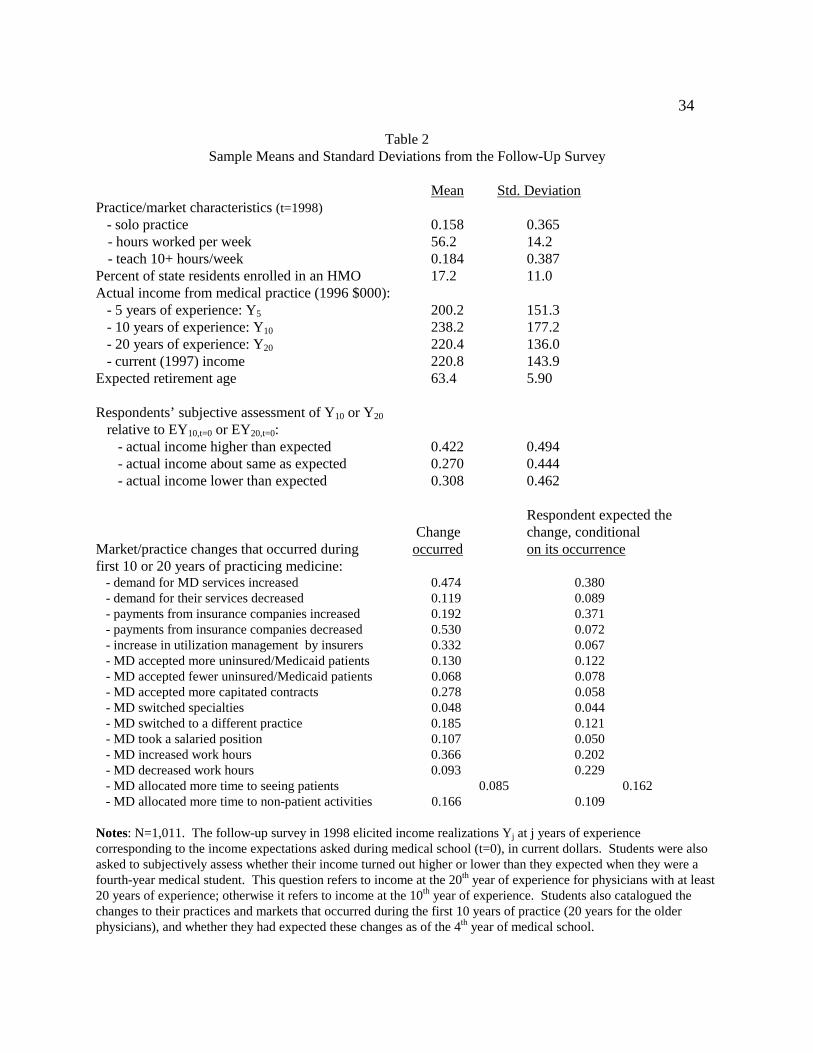
34

Table 2 Sample Means and Standard Deviations from the Follow-Up Survey

Mean Std. Deviation Practice/market characteristics (t=1998) - solo practice 0.158 0.365

- hours worked per week 56.2 14.2 - teach 10+ hours/week 0.184 0.387

Percent of state residents enrolled in an HMO 17.2 11.0 Actual income from medical practice (1996 $000): - 5 years of experience: Y5 200.2 151.3 - 10 years of experience: Y10 238.2 177.2 - 20 years of experience: Y20 220.4 136.0 - current (1997) income 220.8 143.9 Expected retirement age 63.4 5.90 Respondents’ subjective assessment of Y10 or Y20 relative to EY10,t=0 or EY20,t=0: - actual income higher than expected 0.422 0.494 - actual income about same as expected 0.270 0.444 - actual income lower than expected 0.308 0.462 Respondent expected the

Change change, conditional Market/practice changes that occurred during occurred on its occurrence first 10 or 20 years of practicing medicine: - demand for MD services increased 0.474 0.380 - demand for their services decreased 0.119 0.089 - payments from insurance companies increased 0.192 0.371 - payments from insurance companies decreased 0.530 0.072 - increase in utilization management by insurers 0.332 0.067 - MD accepted more uninsured/Medicaid patients 0.130 0.122 - MD accepted fewer uninsured/Medicaid patients 0.068 0.078 - MD accepted more capitated contracts 0.278 0.058 - MD switched specialties 0.048 0.044 - MD switched to a different practice 0.185 0.121 - MD took a salaried position 0.107 0.050 - MD increased work hours 0.366 0.202 - MD decreased work hours 0.093 0.229 - MD allocated more time to seeing patients 0.085 0.162 - MD allocated more time to non-patient activities 0.166 0.109 Notes: N=1,011. The follow-up survey in 1998 elicited income realizations Yj at j years of experience corresponding to the income expectations asked during medical school (t=0), in current dollars. Students were also asked to subjectively assess whether their income turned out higher or lower than they expected when they were a fourth-year medical student. This question refers to income at the 20th year of experience for physicians with at least 20 years of experience; otherwise it refers to income at the 10th year of experience. Students also catalogued the changes to their practices and markets that occurred during the first 10 years of practice (20 years for the older physicians), and whether they had expected these changes as of the 4th year of medical school.

35

T

able

3:

Inco

me

Pre

dict

ion

Err

ors

With

5, 1

0, a

nd 2

0 Y

ears

of

Exp

erie

nce

P

anel

A: A

vera

ge I

ncom

e P

redi

ctio

n E

rror

s (1

996

$000

)

Dep

ende

nt v

aria

ble:

Y5

- E

Y5,

t=0

Y

10 -

EY

10,t=

0

Y20

- E

Y20

,t=0

mea

n (α

0)

107

.6**

9

2.5*

*

2

0.4*

*

S.E

.

(7.1

2)

(6

.04)

(7

.64)

Obs

erva

tions

762

7

53

246

P

anel

B: D

istr

ibut

ion

of I

ncom

e P

redi

ctio

n E

rror

s (1

996

$000

)

Per

cent

ile

Y5

- E

Y5,

t=0

Y

10 -

EY

10,t=

0

Y20

- E

Y20

,t=0

10

th

-

16.2

-

50.9

-1

37.4

25th

20.9

-4.

7

-

77.4

Med

ian

68

.3

4

8.9

5

.9

75

th

1

45.6

1

37.0

74

.1

90

th

2

59.2

2

94.1

202

.3

N

otes

: In

com

e pr

edic

tion

erro

rs a

re c

onst

ruct

ed a

s th

e di

ffer

ence

bet

wee

n ac

tual

inco

me

Yj w

ith

j yea

rs o

f ex

peri

ence

(fr

om th

e fo

llow

-up

surv

ey)

and

the

corr

espo

ndin

g ex

pect

ed in

com

e E

Yj,t

=0 f

or y

ear

j, as

for

ecas

ted

in th

e fo

urth

yea

r of

med

ical

sch

ool (

t=0)

. E

xpec

ted

and

real

ized

inco

mes

are

con

vert

ed to

199

6 do

llar

s us

ing

the

cons

umer

pri

ce in

dex.

Pan

el A

est

imat

es th

e av

erag

e fo

reca

st e

rror

usi

ng e

quat

ion

(1),

by

regr

essi

ng th

e er

rors

on

a co

nsta

nt α

0. T

he s

tand

ard

erro

rs a

re a

djus

ted

to a

llow

for

cor

rela

tion

bet

wee

n ph

ysic

ians

acc

ordi

ng to

the

year

in w

hich

inco

me

was

rec

eive

d. *

* =

sig

nifi

cant

ly d

iffe

rent

fro

m z

ero

at th

e fi

ve-p

erce

nt le

vel.

36

Table 4 Determinants of Income Prediction Errors

(1) (2) (3) (4) Personal Year Specialty Specialty, Year, & Characteristics Controls Controls Personal Characteristics Female -53.5** -49.6** (13.2) (13.8) White 42.7 62.9** (28.2) (26.1) Board score 0.0961 -0.069 (0.290) (0.272) Experience 1.45 -3.50 1.30 -3.06 (1.95) (3.15) (1.96) (2.96) Experience squared -0.295** -0.117 -0.287** -0.079 (0.084) (0.118) (0.084) (0.114) Indicators for year Not included Jointly sig. Not included Jointly significant income received Specialty indicators (family practice omitted) - internal medicine 57.6** 55.6** (10.4) (11.0)

- internal medicine sub-specialties 209** 207** (30.7) (29.3)

- pediatrics 23.3** 25.4** (10.4) (11.1)

- surgery 129** 123** (16.2) (16.7)

- ob/gyn 110** 115** (18.9) (19.8)

- psychiatry 4.02 -3.48 (11.8) (13.1)

- anesthesiology 179** 182** (37.6) (38.2)

- radiology 143** 140** (18.6) (17.8) - pathology 32.7** 27.6*

(14.6) (15.6) - other 72.5** 68.3** (22.1) (22.7) Constant 51.7 126.6** 26.4** 11.6 (63.1) (26.6) (11.6) (67.1) Observations 1,761 1,761 1,761 1,761 R2 0.04 0.05 0.17 0.19 Notes: This table tests for systematic components in the income prediction errors, following equations (2) and (3). The dependent variable is the difference between realized and expected income, Yj – EYj,t=0 in year j. Observations

37 are pooled for j= 5, 10, and 20 years of experience. Family practice is the omitted specialty in columns (3) and (4). Standard errors are corrected to allow the error terms to be correlated for an individual throughout his career. ** = significantly different from zero at the 5-percent level; * = significantly different from zero at the 10-percent level.

38

Table 5

Determinants of Physicians’ Income

Pooled Observations 1997 Income

Coefficient S.E. Coefficient S.E

Female -75.5** 10.0 -54.7** 10.2 White 18.0 20.9 -9.64 31.4 Board score 0.0157 0.255 0.222 0.343 Experience 13.4** 2.59 5.06 7.75 Experience squared -0.461** 0.0792 -0.172 0.227 Percentage of population -0.576 0.627 enrolled in HMO Non-primary care specialty 101** 13.0 60.1** 9.07 (primary care omitted) HMO * non-primary care -1.38** 0.471

Practice characteristics (1998) - hours worked/week 2.09** 0.418 - poor patients as percentage of total -1.10** 0.202 - > 9 hours/week on teaching/research 111 173 - board score * teach > 9 hours -0.667 0.818 - solo practice -44.5** 13.8 - employed by government -87.5** 16.4 Constant 125** 60.9 37.8 103 Observations 2,956 796 R2 0.12 0.18 Notes: The dependent variable is ex post income received in year j, Yij, following equation (4). In the first specification, j is the year in which a physician had 5, 10, and 20 years of experience, pooled together. The standard errors are corrected to allow the errors to be correlated for a physician throughout his career. The second specification uses income only from 1997, the year before the follow-up survey, and includes contemporaneous practice characteristics as of the follow-up survey. Primary care specialties (family practice, pediatrics, and general internal medicine) are the omitted specialties. Indicator variables for the year in which a respondent received his income are included in the both specifications. ** = significantly different from zero at the 5-percent level; * = significantly different from zero at the 10-percent level.

39

Table 6

Effect of HMOs on Income Prediction Errors

Coefficient S.E.

Female -46.5** 13.3 White 62.8** 31.7 Board score 0.102 0.287 Experience -3.41 3.14 Experience squared -0.134 0.117 Non-primary care specialty 88.7** 14.0 (primary care specialties omitted) Percentage of state population 0.407 0.923 enrolled in an HMO HMO * non-primary care -1.89** 0.752 Constant 38.9 76.5 Observations 1,761 R2 0.10

Notes: This table tests for systematic components in the income prediction errors, following equations (2) and (3), focusing on the effect of the growth in health maintenance organization (HMO) enrollment. The dependent variable is the difference between realized and expected income, Yj – EYj,t=0 in year j. Observations are pooled for j= 5, 10, and 20 years of experience. Primary care specialties (family practice, pediatrics, and general internal medicine) are the omitted specialties. Indicator variables are included for the year in which income was received. Standard errors are corrected to allow the errors to be correlated for a physician throughout his career. ** = significantly different from zero at the 5-percent level; * = significantly different from zero at the 10-percent level.

40

Table 7 Impact of Market and Practice Changes on Income Prediction Errors

Anticipated at t=0 Unanticipated at t=0

Market and practice changes: Coefficient S.E. Coefficient S.E. Demand for MD’s services increased 52.7** 18.3 33.1** 15.6 Demand for MD’s services decreased -37.6 57.7 -31.9 21.2 Payments from insurance companies increased 12.1 26.3 43.2* 22.4 Payments from insurance companies decreased 87.4** 37.1 34.5** 14.9 Increase in utilization mgmt by insurers 41.4 51.4 1.18 15.4 MD accepted more uninsured/Medicaid pts 11.7 32.6 -48.8** 16.9 MD accepted fewer uninsured/Medicaid pts 137 139 -74.1** 28.7 MD accepted more capitated contracts -38.8 36.9 -16.1 14.0 MD switched to higher-paying specialty 128** 53.9 MD switched to lower-paying specialty -74.9** 35.3 MD switched to a different practice -6.86 39.7 9.79 15.9 MD took a salaried position -53.2 51.8 -11.5 15.9 MD increased work hours -15.7 25.5 13.5 14.2 MD decreased work hours 8.64 42.9 -3.15 23.4 MD allocated more time to seeing pts 2.13 58.1 21.7 15.2 MD allocated more time to non-pt activities -61.1** 28.1 -34.2** 17.3 Female -46.2** 17.2 White -24.9 55.5 Board score 0.137 0.350 10 years of experience (20 years is omitted) 71.6 19.7 Constant -12.0 86.1 Observations 736 R2 0.15

Notes: This table analyzes the effect on income prediction errors of various changes in physician markets and practices, following equation (3). The dependent variable is the income prediction error in year j: Yj - EYj,t=0. Observations are pooled for j = 10 years or 20 years of experience. We include separate indicator variables for anticipated (at time t=0) market and practice changes, and unanticipated market and practice changes, so the omitted group is physicians who did not experience a particular change. The anticipated and unanticipated changes are both included as independent variables in a single regression; the unanticipated changes are listed in the third column for clarity. Indicator variables are included for the year in which a physician received his income. ** = significantly different from zero at the 5-percent level; * = significantly different from zero at the 10-percent level.

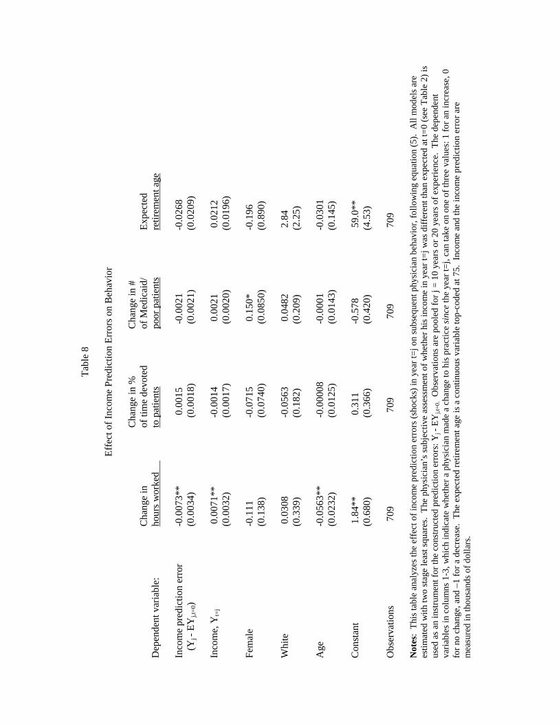
Tab

le 8

Eff

ect o

f In

com

e P

redi

ctio

n E

rror

s on

Beh

avio

r

C

hang

e in

%

C

hang

e in

#

Cha

nge

in

of

tim

e de

vote

d

of M

edic

aid/

Exp

ecte

d

Dep

ende

nt v

aria

ble:

hour

s w

orke

d

to p

atie

nts

po

or p

atie

nts

re

tirem

ent a

ge

In

com

e pr

edic

tion

erro

r

-0.0

073*

*

0

.001

5

-0.

0021

-0.0

268

(Yj -

EY

j,t=

0)

(0.0

034)

(

0.00

18)

(

0.00

21)

(0

.020

9)

Inco

me,

Yt=

j

0

.007

1**

-0.

0014

0.

0021

0.0

212

(0.0

032)

(

0.00

17)

(

0.00

20)

(0

.019

6)

Fem

ale

-0

.111

-0.

0715

0.

150*

-0.1

96

(0.1

38)

(

0.07

40)

(

0.08

50)

(0

.890

)

Whi

te

0

.030

8

-0.

0563

0.

0482

2.8

4

(0

.339

)

(0.

182)

(0.

209)

(2.2

5)

A

ge

-0

.056

3**

-0.

0000

8

-0.

0001

-0.0

301

(0

.023

2)

(0.

0125

)

(0.

0143

)

(0.1

45)

Con

stan

t

1

.84*

*

0.3

11

-

0.57

8

5

9.0*

*

(0.6

80)

(

0.36

6)

(

0.42

0)

(4

.53)

Obs

erva

tions

7

09

709

7

09

709

Not

es:

Thi

s ta

ble

anal

yzes

the

effe

ct o

f in

com

e pr

edic

tion

erro

rs (

shoc

ks)

in y

ear

t=j o

n su

bseq

uent

phy

sici

an b

ehav

ior,

fol

low

ing

equa

tion

(5).

All

mod

els

are

esti

mat

ed w

ith

two

stag

e le

ast s

quar

es.

The

phy

sici

an’s

sub

ject

ive

asse

ssm

ent o

f w

heth

er h

is in

com

e in

yea

r t=

j was

dif

fere

nt th

an e

xpec

ted

at t=

0 (s

ee T

able

2)

is

used

as

an in

stru

men

t for

the

cons

truc

ted

pred

ictio

n er

rors

: Yj -

EY

j,t=0

. O

bser

vatio

ns a

re p

oole

d fo

r j =

10

year

s or

20

year

s of

exp

erie

nce.

The

dep

ende

nt

vari

able

s in

col

umns

1-3

, whi

ch in

dica

te w

heth

er a

phy

sici

an m

ade

a ch

ange

to h

is p

ract

ice

sinc

e th

e ye

ar t=

j, ca

n ta

ke o

n on

e of

thre

e va

lues

: 1 f

or a

n in

crea

se, 0

fo

r no

cha

nge,

and

–1

for

a de

crea

se.

The

exp

ecte

d re

tire

men

t age

is a

con

tinu

ous

vari

able

top-

code

d at

75.

Inc

ome

and

the

inco

me

pred

ictio

n er

ror

are

mea

sure

d in

thou

sand

s of

dol

lars

.

0

20

40

60

80

100

120

140

160

180

200

79/8

081

/82

83/8

485

/86

87/8

889

/90

91/9

293

/94

95/9

697

/98

Fig

ure

1

Dif

fere

nces

in

Inco

me

Pre

dic

tio

n E

rror

s B

etw

een

Pri

mar

y an

d N

on-p

rim

ary

Car

e P

hysi

cian

s

Inco

me

Pre

dic

tion

Err

or

(199

6 $0

00)

Yea

r in

Whi

ch I

ncom

e W

as R

ecei

ved

(2-y

ear

bin

s)

Non

-pri

mar

y ca

re M

Ds

Pri

mar

y ca

re M

Ds

Not

es:

Thi

s fi

gu

re d

ispl

ays

the

year

eff

ects

(in

tw

o-ye

ar b

ins)

fro

m a

reg

ress

ion

of t

he

inco

me

pre

dict

ion

err

ors

Yj-

EY

j,t=

0on

in

dica

tor

vari

able

sfo

r th

e ye

ar i

n w

hic

h in

com

e w

as r

ecei

ved

, an

d in

tera

ctio

ns

of t

he y

ear

dum

mie

s an

d a

n in

dica

tor

for

non

-pri

mar

y ca

re s

peci

alti

es

(e.g

., su

rger

y, i

nter

nal

med

icin

e su

bsp

ecia

ltie

s, o

b/g

yn,

rad

iolo

gy,

an

esth

esio

log

y, p

sych

iatr

y, p

ath

olog

y).

Exp

erie

nce

an

d ex

per

ien

ce s

quar

ed

are

incl

ud

ed i

n th

e re

gre

ssio

n.

Tw

o-ye

ar p

erio

ds w

ith

few

er t

han

30

inc

ome

obse

rvat

ion

s ar

e n

ot d

isp

laye

d in

thi

s fi

gure

.

Appendix: Survey of Jefferson Medical College Alumni, Graduating Classes of 1970-1979

PART A: CHARACTERISTICS OF YOUR PRACTICE We would like to begin with some background information about your current medical practice. 1. Are you working full-time, part-time, or not working at this time?

(01) Full-time (02) Part-time

(03) Not presently working ⇒ Go to Question 9 2. Which of the following best describes your primary employer? (select only one) (01) Solo practice (02) Same-specialty group practice with two or more physicians (03) Multi-specialty group practice with two or more physicians (04) Medical school or hospital (05) Government (city, county, state, or federal, including uniformed services) (06) Other, please specify: ________________________________________ 3. In your primary employment setting, are you a salaried employee, or are you self-employed or a partner? (01) Salaried employee (02) Self-employed or a partner 4. Please indicate your current main specialty and sub-specialty, if any.

Main specialty: _____________________ Sub-specialty: _____________________

5. Thinking about a typical week during 1997, how many hours per week did you devote to

each of the following activities: a. Patient care (including administration of your practice) ____ hours/week b. Teaching and research ____ hours/week c. Administration, other than administration of your own practice (e.g., hospital committees, professional societies) ____ hours/week d. Other, please specify: ______________________ ____ hours/week

TOTAL HOURS per week spent on all professional activities

hours/week 6. Do you consider your practice to be located in a socioeconomically deprived area? (01) Yes (02) No

7. Please estimate the percentage of your patients with the following types of insurance: a. Traditional indemnity plan (e.g., Blue Cross) or self-paying uninsured ____ % b. Managed care: HMO and PPO ____ % c. Medicare (including Medicare HMOs) ____ %

d. Medicaid (including Medicaid HMOs) ____ % e. Uninsured who do not pay ____ % f. Other, please specify: _______________________ ____ %

TOTAL = 100%

PART B: DEVELOPMENTS IN PHYSICIANS’ PRACTICES AND INCOME

This section examines how physicians’ practices and income have changed as their careers progressed through changes in the health care environment.

• Please provide your BEST ESTIMATE to questions concerning income. • All information collected in this survey will be STRICTLY CONFIDENTIAL. The information will be used for research purposes only and will be presented in summary tabulations, never on an individual basis. 8. Please estimate your income from medical practice in 1997 to the nearest $10,000, after

professional expenses but before taxes. Please include all income from fees, salaries, risk pools, retainers, bonuses and other forms of compensation.

Income from medical practice in 1997 $_____________

9. In “Box A” below, please write the year in which you completed all of your post-graduate training, which includes residencies, fellowships, and post-doctorate positions. In “Box B”, add 20 years to the year in Box A. Box A: Year completed post-graduate training Box A

Box B: 20 years after completing post-graduate training Box B Please try to recall your medical practice 20 years after you completed post-graduate training (the year indicated in Box B of Question 9). 10. IN YOUR 20th YEAR of practicing medicine, what was your income from medical practice,

after professional expenses but before taxes? (Don’t adjust for inflation; report the dollar amount you actually received in that year).

Income from medical practice 20 years after completing post-graduate training $_____________

11. What about two earlier points in the past: 10 YEARS and 5 YEARS after you completed post-graduate training

(10 years and 5 years after the year in Box A)? For each of these two years, please estimate your income from medical practice, after professional expenses but before taxes. (Again, don’t adjust for inflation; report the dollar amount you actually received in each of these two years).

Income from medical practice 10 years after completing post-graduate training

$______________ Income from medical practice 5 years after completing post-graduate training

$______________ Next, try to recall your experiences leading up to your 20th year of practicing medicine. 12. Were there any CHANGES IN THE HEALTH CARE ENVIRONMENT that had a

significant effect on your practice income in your 20th year (the year in Box B)? (Please include changes that occurred anytime in your first 20 years of practicing medicine that continued to have a significant effect in your 20th year). Please circle all that apply.

A. Demand increased (e.g., an increase in patients per physician in my market) B. Demand decreased (e.g., a decline in patients per physician in my market) C. Fees increased from insurance companies and the government D. Fees decreased from insurance companies and the government E. I accepted more uninsured or Medicaid patients in my practice F. I accepted fewer uninsured or Medicaid patients in my practice G. Capitated contracts (fixed payment per patient) became more prevalent in my

practice H. Utilization management by insurance companies increased (e.g., disease

management protocols) I. Other, please specify: ______________________________________________

13. Did you make any CHANGES TO YOUR PRACTICE that had a significant effect on your practice income in your 20th year? (Include changes that you made anytime in your first 20 years of practicing medicine that continued to have a significant effect in your 20th year). Please circle all that apply.

J. I switched specialties K. I switched to a different practice (either in the same city or a different city) L. I switched to a salaried position with a physician group practice, HMO, or health

system M. I sold my practice

N. I increased the number of hours I worked O. I reduced the number of hours I worked P. I spent more of my time seeing patients, less on other activities (e.g.,

teaching/research) Q. I spent less of my time seeing patients, more on other activities (e.g.,

teaching/research) R. Other, please specify: _______________________________________________

14. Think about the changes that you circled in Questions 12 and 13. Which of these changes would you say you had expected in advance when you were a fourth-year medical student? Please circle the letters below that correspond to previously expected changes: A. B. C. D. E. F. G. H. I. J. K. L. M. N. O. P. Q. R. S. None of the changes circled in Questions 12 and 13 was expected 15. Overall, how did your ACTUAL practice income in your 20th year compare with the 20th year

income that you had EXPECTED when you were a fourth-year medical student (after taking inflation into consideration)?

(01) Actual income after 20 years was higher than previously expected (02) Actual income after 20 years was lower than previously expected (03) Actual income after 20 years was about the same as previously expected

Finally, think about events that have affected your medical practice in more recent years. 16. In the time SINCE YOUR 20th YEAR of practicing medicine (the years after Box B), have you made any substantial changes to your medical practice? Please check all that apply. (01) I switched specialties (02) I switched to a different practice (either in the same city or a different city)

(03) I switched to a salaried position with a physician group practice, HMO, or health system

(04) I sold my practice (05) I increased the number of hours I work

(06) I reduced the number of hours I work (07) I spent more of my time seeing patients, less on other activities (e.g., teaching/research) (08) I spent less of my time seeing patients, more on other activities (e.g.,

teaching/research) (09) I increased the number of Medicaid or uninsured patients in my practice (10) I reduced the number of Medicaid or uninsured patients in my practice (11) I accepted more capitated contracts (12) I accepted fewer capitated contracts (13) Other, please specify ___________________________________ (14) I did not made any substantial changes to my practice in recent years

PART C: EXPECTATIONS ABOUT THE FUTURE We are interested in how changes in the health care environment are affecting physicians’ expectations of their practices and income in the future. 17. FIVE YEARS FROM NOW, do you think you will be practicing medicine or will you be fully retired?

I expect to be practicing medicine in 5 years ⇒ Go to Question 18 I expect to be fully retired from medicine in 5 years ⇒ Go to Question 20

18. How many hours per week do you expect to be working in 5 years? ________ hours/week 19. Looking ahead, what do you think your annual income from medical practice will be in 5 years, after professional expenses, but before taxes? (Don’t adjust for inflation; assume that dollars maintain their current value.)

Income from medical practice expected in 5 years $_____________ 20. At what age do you expect to retire completely from medicine? (If you have already retired, please indicate your age at retirement)

Age when you expect to retire __________ years old

THANK YOU for taking the time to complete our survey.