Income Polarization in Brazil, 2001-2011: A Distributional

Analysis Using PNAD Data

Fabio Clementi (University of Macerata, Italy)

Francesco Schettino (Second University of Naples, Italy)

Paper Prepared for the IARIW-IBGE Conference

on Income, Wealth and Well-Being in Latin America

Rio de Janeiro, Brazil, September 11-14, 2013

Session 10: Income Distribution in Latin America

Time: Friday, September 12, 2:00-3:30

INCOME POLARIZATION IN BRAZIL, 2001–2011: ADISTRIBUTIONAL ANALYSIS USING PNAD DATA

Fabio Clementi and Francesco Schettino

This paper applies a non-parametric tool, the “relative distribution”, to iden-tify patterns of changes in Brazil’s household income distribution over the period2001–2011. Despite the sharp decline in income inequality recently experienced bythe country, we are able to document an increased income polarization, which hasparticularly affected households below the median. The results call directly into ques-tion the future sustainability and equity of existing social programs dealing with theunequal distribution of resources.

Keywords: Brazil, income distribution, relative distribution, polarization.

1. INTRODUCTION

Brazil has long been known as one of the countries with the most unequalincome distribution in the world. The concentration of incomes in 1960 wasalready high by international standards, as indicated by a Gini coefficient of0.504, and continued to increase in the following decades (Lopez-Calva, 2012).Income inequality only declined starting in the mid-1990s: after 1997, the Ginireduced by 0.8% per year; between 2001 and 2007, the average rate of annualdecline accelerated to 1.2%, well above the pace of the Latin American region asa whole (Barros et al., 2010). Poverty in the country also declined significantlyduring the last decade: the absolute number of poor people fell from over 61million in 2003 to under 40 million in 2009 and the headcount index from 35.8%to 21.4% (Higgins, 2012). Meanwhile, Brazil’s GDP growth managed to overtakethe UK as the world’s sixth-largest economy in 2011 (CEBR, 2011).Although several factors contributed to the recent progress in terms of poverty

and inequality reduction—such as economic growth (Barros et al., 2010), ex-panded access to education during the 1990s (Gasparini and Lustig, 2011), in-creased demand for unskilled labour (Robinson, 2010) and an increase in theminimum wage (Barros, 2007), it is common opinion that the conditional cashtransfer (CCT) programs consolidated and expanded under the administration ofthe former Brazilian president Luiz Inacio Lula da Silva (2003–2010) have alsoplayed an important role.1 Notwithstanding many critical remarks—focusing

Department of Political Science, Communication and International Relations, University ofMacerata, Piazza G. Oberdan 3, 62100 Macerata, Italyfabio.clementi@unimc.it

Department of Law, Second University of Naples, Via Mazzocchi 5, 81055 S. Maria CapuaVetere, Italyfrancesco.schettino@unina2.it

1CCTs are direct monetary transfers provided to poor families on condition that they ensurechildren and adolescents attend school and that they meet basic health care requirements.These conditions attempt both to reduce short-term poverty by direct cash transfers and tofight long-term poverty by investing in the human capital of the poor (see e.g. Fiszbein et al.,2009.)

1

2 F. CLEMENTI AND F. SCHETTINO

principally on the high related costs,2 CCTs received the appreciation by inter-national institutions and were enthusiastically embraced by many countries as amajor social policy instrument (Hall, 2006). “Bolsa Famılia” is now the largestsuch scheme in the world: it was budgeted at R$8.3 billion (equivalent to almost0.4% of GDP) in 2006 and covered around 11 millions families (approximately46 millions people) over the same year (Lindert et al., 2007). As a result of theirexcellent targeting, the program’s benefits accounted for something between 21%and 16% of the total fall in Brazilian inequality since 2001 (Soares, 2012). Thedecline in inequality has been crucial for poverty reduction (accounting for halfof the total change between 2001 and 2009) and certainly for making growthfriendlier to the poor (Lopez-Calva and Rocha, 2012).

The recent trend in terms of inequality changes is unique in respect to what isbeing experienced in Brazil’s fellow BRICS countries: Russia, India, China andSouth Africa (OECD, 2011). However, while there is a substantial literature oninequality and income distribution in Brazil (both in isolation and in a compar-ative perspective; see e.g. World Bank, 2004, and references therein) relativelylittle work has been done in terms of analyzing changes in the shape of Brazil’sincome distribution in the recent decade. Indeed, the above mentioned evidenceheavily relies on summary measures of inequality and not on the whole shape ofthe income distribution. As noted by Morris et al. (1994), standard measures ofinequality may suggest a particular outcome in terms of inequality change—e.g.a fall in the Gini coefficient or Theil index—while implying a radically differentpattern of distributional change. In particular, they may not capture aspectssuch as multi-modality and polarization.

In seeking to understand exactly how income inequality fell in Brazil over thelast decade, in the present study we look “behind” the usual summary mea-sures and closely examine the patterns of changes that have occurred along theentire Brazilian income distribution. More specifically, it is our aim to inves-tigate whether the favourable combination of economic growth and inequalityreduction—from which the country has benefited during the last 15 years orso—has produced significant movements across the income scale, and whetherthese movements have taken the form of a convergence of the top and bot-tom percentiles toward the middle income class or of a shrinking of the lat-ter—thereby leading to greater distributional polarization. For this purpose, weapply a non-parametric tool, the “relative distribution”, to survey income data(PNAD) spanning 2001–2011 and covering a large number of households acrossall federal units of Brazil.

The remainder of this paper is structured as follows: Section 2 is devotedto the illustration of the main features of income data; Section 3 reviews therelative distribution method; Section 4 details the results and findings; Section5 concludes and draws some policy implications.

2For a review see in particular Coggiola (2010).

INCOME POLARIZATION IN BRAZIL 3

2. DATA AND SUMMARY STATISTICS

We use data from Brazil’s annual national household survey (Pesquisa Na-cional por Amostra de Domiclios, PNAD) for 2001 to 2011.3 The PNAD iscollected every year in September—except in 2010—by the National Census Bu-reau (Instituto Brasileiro de Geografia e Estatstica, IBGE) and is nationallyrepresentative at the level of each state. However, until 2003 the PNAD wasnot representative for the rural areas of the North region (minus the state ofTocantins). Therefore, in order to maintain time-series comparable these areaswere excluded from PNAD data for 2004 onward. In this way, our samples haveon average about 107,000 observations a year.

All calculations are based on total household income expressed in BrazilianReais (R$). Current values have been deflated using the consumer price index(yearly series based on 2005) reported by the OECD.4 Furthermore, incomeshave been equivalized for differences in household size5 and weighted by usingappropriate sampling weights provided by the IBGE staff.

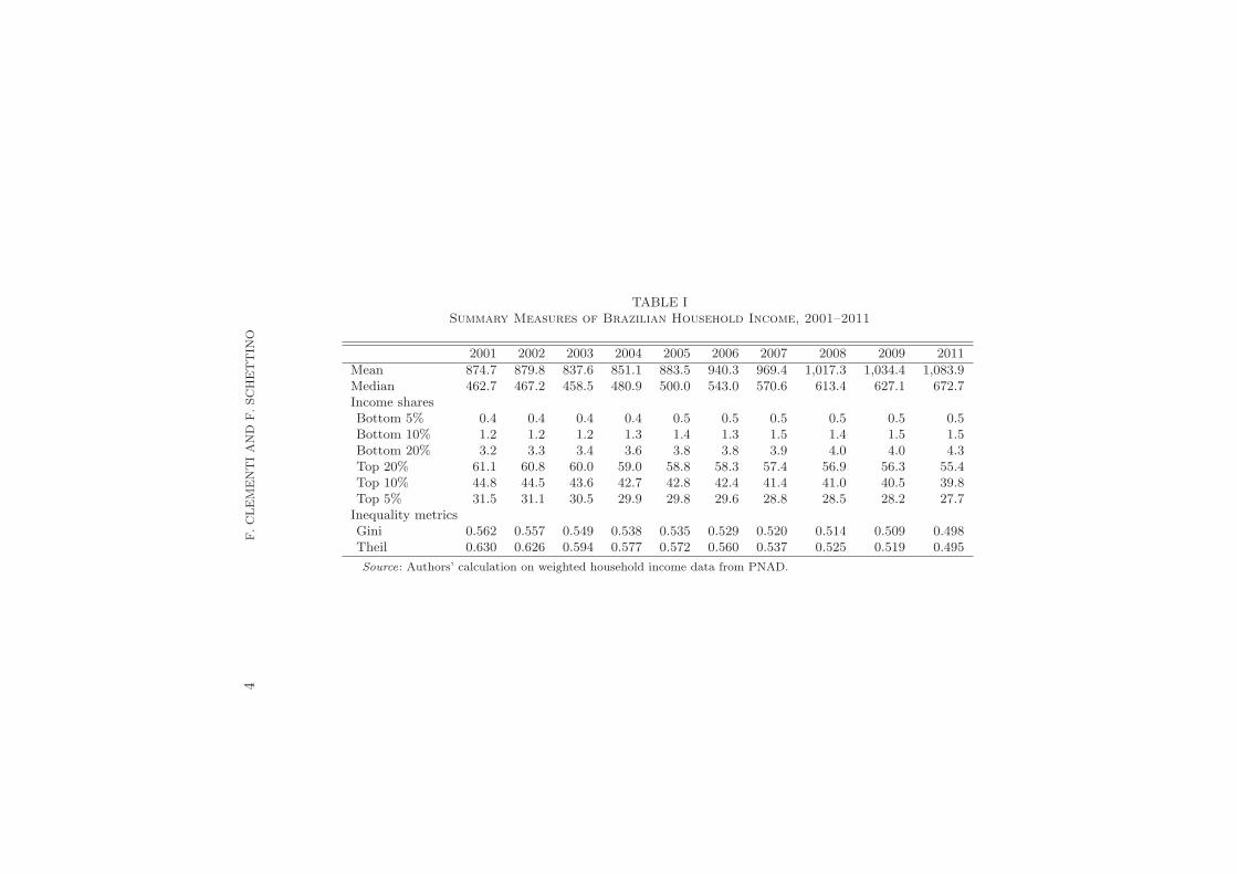
Table I provides summary measures for annual household income from 2001to 2011. Besides the growth of the real mean and median incomes, the mostnotable feature is that income shares of the poorest percentiles of the populationincreased on average between approximately 2% and 3% per year in the periodexamined, on the contrary of what observed for the richest percentiles whoseshares decreased by around 1% or more. As for inequality, the improvements werealso noticeable: the Gini and Theil indices exhibited nearly the same temporalprofile, showing an average yearly decrease that amounts respectively to 1% and2%.

All these figures seem to be consistent with the positive (and sometimes en-thusiastic) evaluation of Brazil’s economic and social policies under the formerPresident Lula’s administration. But while suggesting important candidate ex-planations for the distributional change, the statistics reported do not capturethe other changes that might have occurred. In particular, the key questions arehinted at but not easily quantified using the standard measures here. How wellare the differences captured by simple location shifts? Is there evidence of grow-ing polarization? Are the upper and lower tails of the distributions changing insimilar ways? As mentioned in the previous section, in this paper we propose anapplication based on the “relative distribution”, a non-parametric statistical toolfor fully representing differences between distributions that we deem well-suitedto deal with the above questions.

3The data are publicly available at http://www.ibge.gov.br/english/estatistica/

populacao/trabalhoerendimento/pnad2011/default.shtm.4Available at http://stats.oecd.org/.5Here we adopt a simple equivalence scale that is most commonly used in international

studies (e.g. Atkinson et al., 1995) where total household income is divided by the square rootof the number of household members.

4F.CLEMENTIAND

F.SCHETTIN

O

TABLE ISummary Measures of Brazilian Household Income, 2001–2011

2001 2002 2003 2004 2005 2006 2007 2008 2009 2011

Mean 874.7 879.8 837.6 851.1 883.5 940.3 969.4 1,017.3 1,034.4 1,083.9Median 462.7 467.2 458.5 480.9 500.0 543.0 570.6 613.4 627.1 672.7Income sharesBottom 5% 0.4 0.4 0.4 0.4 0.5 0.5 0.5 0.5 0.5 0.5Bottom 10% 1.2 1.2 1.2 1.3 1.4 1.3 1.5 1.4 1.5 1.5Bottom 20% 3.2 3.3 3.4 3.6 3.8 3.8 3.9 4.0 4.0 4.3Top 20% 61.1 60.8 60.0 59.0 58.8 58.3 57.4 56.9 56.3 55.4Top 10% 44.8 44.5 43.6 42.7 42.8 42.4 41.4 41.0 40.5 39.8Top 5% 31.5 31.1 30.5 29.9 29.8 29.6 28.8 28.5 28.2 27.7Inequality metricsGini 0.562 0.557 0.549 0.538 0.535 0.529 0.520 0.514 0.509 0.498Theil 0.630 0.626 0.594 0.577 0.572 0.560 0.537 0.525 0.519 0.495

Source: Authors’ calculation on weighted household income data from PNAD.

INCOME POLARIZATION IN BRAZIL 5

3. ASSESSING INCOME POLARIZATION IN BRAZIL: THE RELATIVE

DISTRIBUTION APPROACH

Over the last two decades, the issue of polarization has come to be assignedincreasing importance in the analysis of income distribution. Notwithstandingthe pains the polarization literature has suffered to distinguish itself from pureinequality measurement—see e.g. Foster and Wolfson (1992), Levy and Murnane(1992), Esteban and Ray (1994) and Wolfson (1994, 1997), it now seems to befairly widely accepted that polarization is a distinct concept from inequality.

Broadly speaking, the notion of polarization is concerned with the disappear-ance of the middle class, which occurs when there is a tendency to concentrate inthe tails—rather than the middle—of the income distribution. One of the mainreasons for looking at income polarization this way, which is usually referred toas “bi-polarization”, is that a well-off middle class is important to every societybecause it contributes significantly to economic growth, as well as to social andpolitical stability (e.g. Pressman, 2007). In contrast, a society with high degreeof income polarization may give rise to social conflicts and tensions. Therefore,in order for such risks to be minimized, it is necessary to monitor the economicevolution of the society using indices that look at the dispersion of the incomedistribution from the middle toward either or both of the two tails.6 Measuresof income polarization that correspond to this case have been proposed in theliterature by Foster and Wolfson (1992), Wolfson (1994, 1997), Wang and Tsui(2000), Chakravarty and Majumder (2001), Rodrıguez and Salas (2003),Chakravarty et al. (2007), Silber et al. (2007), Chakravarty (2009),Chakravarty and D’Ambrosio (2010), Lasso de la Vega et al. (2010), andothers.

A more general notion of income polarization, which was originally proposedby Esteban and Ray (1994), regards the latter as “clustering” of a populationaround two or more poles of the distribution, irrespective of where they are lo-cated along the income scale. The notion of income polarization in a multi-groupcontext is an attempt at capturing the degree of potential conflict inherent in

6More precisely, there are two characteristics that are considered as being intrinsic to thenotion of bi-polarization. The first one, “increased spread”, implies that moving from thecentral value (median) to the extreme points of the income distribution makes the distributionmore polarized than before. In other words, increments (reductions) in incomes above (below)the median will widen the distribution, that is extend the distance between the groups belowand above the median and hence increase the degree of bi-polarization. On the other hand,“increased bi-polarity” refers to the case where incomes on the same side of the median getcloser to each other. Since the distance between the incomes below or above the median hasbeen reduced, this is assumed to increase bi-polarization. Thus, bi-polarization involves bothan inequality-like component, the “increased spread” principle, which increases both inequalityand polarization, and an equality-like component, the “increased bi-polarity” criterion, whichincreases polarization but lowers any inequality measure that fulfills the Pigou-Dalton transferprinciple—the requirement under which inequality decreases when a transfer is made from aricher to a poorer individual without reversing their pairwise ranking. This shows that althoughthere is complementarity between polarization and inequality, there are differences as well. Seethe references cited in the main text for a thorough discussion.

6 F. CLEMENTI AND F. SCHETTINO

a given distribution (see Esteban and Ray, 1999, 2011). The idea is to considersociety as an amalgamation of groups, where the individuals in a group sharesimilar attributes with the other members (i.e. have a mutual sense of “identi-fication”) but in terms of the same attributes they are different from the mem-bers of the other groups (i.e. have a feeling of “alienation”). Political or socialconflict is therefore more likely the more homogenous and separate the groupsare, that is when the within-group income distribution is more clustered aroundits local mean and the between-group income distance is longer. In addition toEsteban and Ray (1994), indices regarding the concept of income polarization asconflict among groups have been investigated, among others, by Gradın (2000),Milanovic (2000), D’Ambrosio (2001), Zhang and Kanbur (2001), Reynal-Querol(2002), Duclos et al. (2004), Lasso de la Vega and Urrutia (2006), Esteban et al.(2007), Gigliarano and Mosler (2009) and Poggi and Silber (2010).

Much of the literature so far considered has analyzed summary measures ofincome polarization. Another strand uses kernel density estimation and mix-ture models in order to describe changes in polarization patterns over time,not just of personal incomes (as in Jenkins, 1995, 1996, Pittau and Zelli,2001, 2004, 2006, and Conti et al., 2006) but also of the cross-country dis-tribution of per capita income (see Quah, 1996a,b, 1997, Bianchi, 1997,Jones, 1997, Paap and van Dijk, 1998, Johnson, 2000, Holzmann et al., 2007,Henderson et al., 2008, Pittau et al., 2010, Anderson et al., 2012, and others).The analysis of the income distribution shape provides indeed a picture fromwhich at least three important distributional features can be observed simulta-neously (Cowell et al., 1996): income levels and changes in the location of thedistribution as a whole; income inequality and changes in the spread of thedistribution; clumping and polarization as well as changes in patterns of cluster-ing at different modes. Finally, a rather recent (yet non-parametric) approachthat combines the strengths of summary polarization indices with the detailsof distributional change offered by the kernel density estimates—the so-called“relative distribution”—has been employed by Alderson et al. (2005), Massari(2009), Massari et al. (2009a,b), Borraz et al. (2011) and Alderson and Doran(2011, 2013) to assess the evolution of the middle class and the degree of house-hold income polarization in a number of middle- and high-income countries inthe world.

Recalling the objectives of our study, stated in Section 1, we deem that inthe current application the relative distribution approach has some importantadvantages over the other mentioned methods of investigating income polariza-tion. First, it readily lends itself to simple and informative graphical displays ofrelative data that reveal precisely where and by how much an income distribu-tion changed over time. Second, by providing the potential for decompositioninto location and shape components, it allows one to examine several hypothesesregarding the origins of distributional change—such as whether the change wasdue to a proportional variation in all incomes that moved the overall distributioneither back or forth (while leaving the shape unaltered) or to shape modifications

INCOME POLARIZATION IN BRAZIL 7

which, by definition, are independent of location shifts.7 Lastly, it allows to quan-tify the degree of polarization due to changes in distributional shape only (i.e.net of location shifts), thus enabling one to isolate aspects of inter-distributionalinequality that are often hidden when also changes in location are examined.Basically, the relative distribution method can be applied whenever the dis-

tribution of some quantity across two populations is to be compared, eithercross-sectionally or over time.8 To proceed, it is necessary to single out one ofthe two populations, refer to it as the “comparison” population, and refer tothe other as the “reference” population. More formally, let Y0 be the incomevariable for the reference population (e.g. households in 2001) and Y the incomevariable for the comparison population (e.g. households in 2011). The relativedistribution of Y to Y0 is defined as the distribution of the random variable:

(1) R = F0 (Y ) ,

which is obtained from Y by transforming it by the cumulative distribution func-tion of Y0, F0. As a random variable, R is continuous on the outcome space [0, 1],and its realizations, r, are referred to as “relative data”. Intuitively, the relativedata can be interpreted as the set of positions that the income observations ofthe comparison population would have if they were located in the income distri-bution of the reference population. The probability density function of R, whichis called the “relative density”, can be obtained as the ratio of the density of thecomparison population to the density of the reference population evaluated atthe relative data r:

(2) g (r) =f(F−10 (r)

)

f0(F−10 (r)

) =f (yr)

f0 (yr), 0 ≤ r ≤ 1, yr ≥ 0,

where f (·) and f0 (·) denote the density functions of Y and Y0, respectively,and yr = F−1

0 (r) is the quantile function of Y0.9 The relative density has a

simple interpretation, as it describes where households at various quantiles inthe comparison distribution are concentrated in terms of the quantiles of thereference distribution. As for any density function, it integrates to 1 over theunit interval, and the area under the curve between two values r1 and r2 is the

7Of course, both the location and shape effects—named respectively as “growth” and “in-equality” (or “distributional”) effect (Bourguignon, 2003, 2004; Kakwani, 1993)—may alsoconcur together in producing the distributional change.

8Here we limit ourselves to illustrating the basic concepts behind the use of the relativedistribution method. For a systematic introduction we refer the reader to Handcock and Morris(1998, 1999)—see also Hao and Naiman (2010, ch. 5). A method very similar in spirit hasrecently been presented by Silber and Deutsch (2012).

9The income density functions are estimated using a non-parametric kernel method. Oncewe obtain the relative density functions for different realizations of R, we fit a local polynomialto the estimated data points in order to have an accurate description of the relative density.Throughout, we rely on the R statistical package reldist (Handcock, 2011) to implement therelative distribution method.

8 F. CLEMENTI AND F. SCHETTINO

proportion of the comparison population whose income values lie between ther1

th and r2th quantiles of the reference population.

When the relative density function shows values near to 1, it means thatthe two populations have a similar density at the rth quantile of the referencepopulation, and thus R has a uniform distribution in the interval [0, 1]. A relativedensity greater than 1 means that the comparison population has more densitythan the reference population at the rth quantile of the latter. Finally, a relativedensity function less than 1 indicates the opposite. In this way one can distinguishbetween growth, stability or decline at specific points of the income distribution.

As we have said before, one of the major advantages of this method is thepossibility to decompose the relative distribution into changes in location, usuallyassociated with changes in the median (or mean) of the income distribution, andchanges in shape (including differences in variance, asymmetry and/or otherdistributional characteristics) that could be linked with several factors like, forinstance, polarization. Formally, the decomposition can be written as:

(3) g (r) =f (yr)

f0 (yr)︸ ︷︷ ︸

Overall relativedensity

=f0L (yr)

f0 (yr)︸ ︷︷ ︸

Density ratio forthe location effect

×f (yr)

f0L (yr)︸ ︷︷ ︸

Density ratio forthe shape effect

,

where f0L (yr) = f0 (yr + ρ) is a density function adjusted by an additive shiftwith the same shape as the reference distribution but with the median of thecomparison one.10 The value ρ is the difference between the medians of the com-parison and reference distributions. If the latter two distributions have the samemedian, the density ratio for location differences is uniform in [0, 1]. Conversely,if the two distributions have different median, the “location effect” is increasing(decreasing) in r if the comparison median is higher (lower) than the referenceone. The second term, which is the “shape effect”, represents the relative densitynet of the location effect and is useful to isolate movements (re-distribution) oc-curred between the reference and comparison populations. For instance, we couldobserve a shape effect function with some sort of (inverse) U-shaped pattern ifthe comparison distribution is relatively (less) more spread around the medianthan the location-adjusted one. Thus, it is possible to determine whether there ispolarization of the income distribution (increases in both tails), “downgrading”(increases in lower tail), “upgrading” (increases in the upper tail) or convergenceof incomes towards the median (decreases in both tails).

This approach also includes amedian relative polarization index (MRP), whichis based on changes in the shape of the income distribution to account for po-

10Median adjustment is preferred here to mean adjustment because of the well-known draw-backs of the mean when distributions are skewed. A multiplicative median shift can also beapplied. However, the multiplicative shift has the drawback of affecting the shape of the distri-bution. Indeed, the equi-proportionate income changes increase the variance and the rightwardshift of the distribution is accompanied by a flattening (or shrinking) of its shape (see e.g.Jenkins and Van Kerm, 2005).

INCOME POLARIZATION IN BRAZIL 9

larization. This index is normalized so that it varies between -1 and 1, with0 representing no change in the income distribution relative to the referenceyear. Positive values represent more polarization—i.e. increases in the tails ofthe distribution—and negative values represent less polarization—i.e. conver-gence towards the center of the distribution. The MRP index for the comparisonpopulation can be estimated as (Morris et al., 1994, p. 217):

(4) MRP =4

n

(n∑

i=1

∣∣∣∣ri −

1

2

∣∣∣∣

)

− 1,

where ri is the proportion of the median-adjusted reference incomes that are lessthan the ith income from the comparison sample, for i = 1, . . . , n, and n is thesample size of the comparison population.

The MRP index can be additively decomposed into the contributions to overallpolarization made by the lower and upper halves of the median-adjusted rela-tive distribution, enabling one to distinguish downgrading from upgrading. Interms of data, the lower relative polarization index (LRP) and the upper relativepolarization index (URP) can be calculated as follows:

(5) LRP =8

n

n/2∑

i=1

(1

2− ri

)

− 1,

(6) URP =8

n

n∑

i=n/2+1

(

ri −1

2

)

− 1,

with MRP = 12(LRP + URP). As the MRP, LRP and URP range from -1 to 1,

and equal 0 when there is no change.

4. THE RELATIVE DISTRIBUTION ANALYSIS

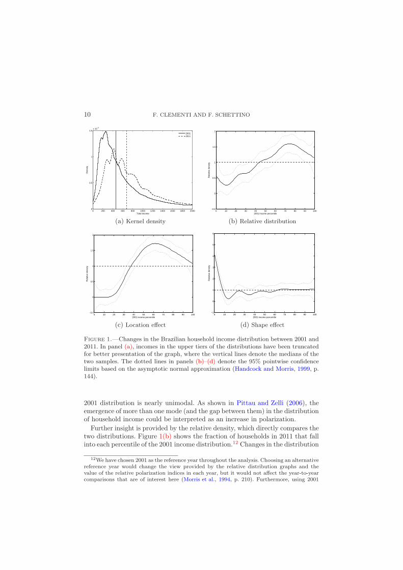
Figure 1(a) presents kernel density estimates of total household income atthe two end points of the 2001–2011 period.11 At first glance, we observe arightward shift of the whole distribution, which implies an increase of the medianincome in this period. The increment in the median can be explained by thesubstantial decline in the mass at the lower and middle income ranges and theconcomitant spreading out of incomes in the top half of the distribution. There isalso a significant alteration of the shape, especially in the middle income range:the 2011 distribution reveals indeed clear evidence of multi-modality, while the

11To handle data sparseness, the two densities have been obtained by using an adaptive ker-nel estimator with a Silverman’s plug-in estimate for the pilot bandwidth (see e.g. Van Kerm,2003). The advantage of this estimator is that it does not over-smooth the distribution in zonesof high income concentration, while keeping the variability of the estimates low where data arescarce—as, for example, in the highest income ranges.

10 F. CLEMENTI AND F. SCHETTINO

0 200 400 600 800 1000 1200 1400 1600 1800 20000

0.5

1

1.5x 10

−3

Total income

Den

sity

20012011

(a) Kernel density

0 10 20 30 40 50 60 70 80 90 100−0.5

0

0.5

1

1.5

2

2001 income percentile

Rel

ativ

e de

nsity

(b) Relative distribution

0 10 20 30 40 50 60 70 80 90 100−0.5

0

0.5

1

1.5

2

2001 income percentile

Rel

ativ

e de

nsity

(c) Location effect

0 10 20 30 40 50 60 70 80 90 100−1

0

1

2

3

4

5

6

2001 income percentile

Rel

ativ

e de

nsity

(d) Shape effect

Figure 1.—Changes in the Brazilian household income distribution between 2001 and2011. In panel (a), incomes in the upper tiers of the distributions have been truncatedfor better presentation of the graph, where the vertical lines denote the medians of thetwo samples. The dotted lines in panels (b)–(d) denote the 95% pointwise confidencelimits based on the asymptotic normal approximation (Handcock and Morris, 1999, p.144).

2001 distribution is nearly unimodal. As shown in Pittau and Zelli (2006), theemergence of more than one mode (and the gap between them) in the distributionof household income could be interpreted as an increase in polarization.

Further insight is provided by the relative density, which directly compares thetwo distributions. Figure 1(b) shows the fraction of households in 2011 that fallinto each percentile of the 2001 income distribution.12 Changes in the distribution

12We have chosen 2001 as the reference year throughout the analysis. Choosing an alternativereference year would change the view provided by the relative distribution graphs and thevalue of the relative polarization indices in each year, but it would not affect the year-to-yearcomparisons that are of interest here (Morris et al., 1994, p. 210). Furthermore, using 2001

INCOME POLARIZATION IN BRAZIL 11

are indicated by the generally positive slope of the relative density, which impliesa decrease of the mass of households below the 2001 median income over theperiod under consideration. More specifically, the relative distribution is less than1 for r ≤ 0.44 and more than 1 for r > 0.44. This means that if we choose anypercentile between the 1st and the 44th in the 2001 distribution, the fraction ofhouseholds in 2011 that earn an amount of income corresponding to the chosenpercentile is less than the analogous fraction of households in 2001. However,income growth between 2001 and 2011 also positively affected households in thetop half of the distribution: the peak of 1.6 is at around the 75th percentile,meaning that households in 2011 are approximately 60% more likely to fall atthe level of 2001 income corresponding to the 75th percentile than households in2001.

To get a more detailed picture, we decompose the relative density into locationand shape effects according to Equation (3). Figure 1(c) presents the effect onlydue to the median shift, that is the pattern that the relative density would havedisplayed if there had been no change in distributional shape but only a locationshift of the density. Since the median shift is positive, the location effect reducesthe share of households in bottom percentiles and increases that in the higherones, hence confirming our prior observation. Figure 1(d) shows the shape effect,which represents the relative density net of the median influence. The visualimpression that one gets from the figure above indicates a marked change forincomes below the median, with a decline of the mass between approximately the9th and the 63th percentile and a prominent increase of the fraction of householdsat the poorest decile of the distribution. This means that while the vast majorityof households experienced a growth in their real income, the poorest fraction ofthem failed to catch up with the rest of population. On the contrary, the upperpart of the relative density does not reveal significant changes, apart from a slightincrease of the mass between the 67th and the 76th percentile and an almost equalincrease at the very top income range from the 92th percentile onward.

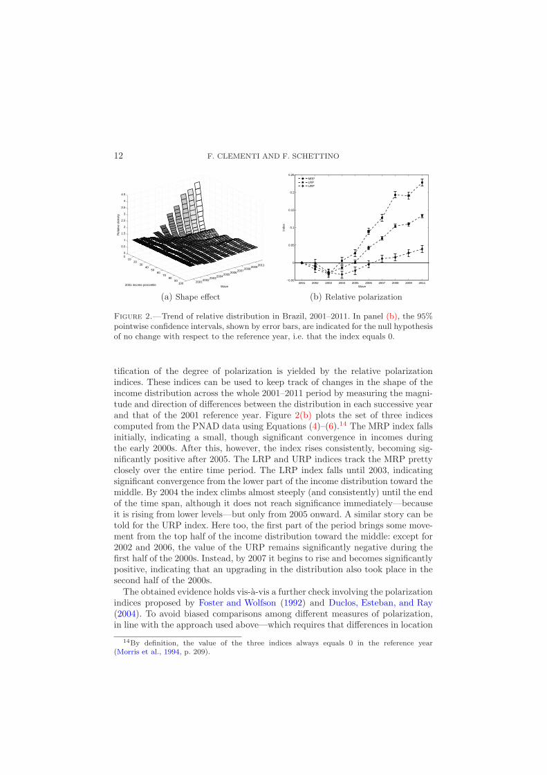
The relative distribution method permits us to also analyze how income re-distribution across households took place during 2001 to 2011. For each yearwithin this period, Figure 2(a) shows the shape effect of the household incomerelative densities using 2001 as the reference year.13 Following the plot througheach successive year, one is offered with the immediate impression that the frac-tion of households in the bottom income levels increased consistently by themid-2000s, while the fraction in the middle and the upper declined. However,toward the end of the first decade of 2000s a moderate growth in upper in-come levels is also apparent, which indicates that the distribution is beginningto polarize.

A link between what we have observed in the graphical analysis and the quan-

as the reference year allows us to examine the longest span available in the PNAD series forBrazil.

13The relative distribution, and therefore its shape effect, is by definition flat in the referenceyear (Morris et al., 1994, p. 211).

12 F. CLEMENTI AND F. SCHETTINO

20012002

20032004

20052006

20072008

20092011

10090

8070

6050

4030

2010

00

0.5

1

1.5

2

2.5

3

3.5

4

4.5

Wave2001 income percentile

Rel

ativ

e de

nsity

(a) Shape effect

2001 2002 2003 2004 2005 2006 2007 2008 2009 2011−0.05

0

0.05

0.1

0.15

0.2

0.25

WaveIn

dex

MRPLRPURP

(b) Relative polarization

Figure 2.—Trend of relative distribution in Brazil, 2001–2011. In panel (b), the 95%pointwise confidence intervals, shown by error bars, are indicated for the null hypothesisof no change with respect to the reference year, i.e. that the index equals 0.

tification of the degree of polarization is yielded by the relative polarizationindices. These indices can be used to keep track of changes in the shape of theincome distribution across the whole 2001–2011 period by measuring the magni-tude and direction of differences between the distribution in each successive yearand that of the 2001 reference year. Figure 2(b) plots the set of three indicescomputed from the PNAD data using Equations (4)–(6).14 The MRP index fallsinitially, indicating a small, though significant convergence in incomes duringthe early 2000s. After this, however, the index rises consistently, becoming sig-nificantly positive after 2005. The LRP and URP indices track the MRP prettyclosely over the entire time period. The LRP index falls until 2003, indicatingsignificant convergence from the lower part of the income distribution toward themiddle. By 2004 the index climbs almost steeply (and consistently) until the endof the time span, although it does not reach significance immediately—becauseit is rising from lower levels—but only from 2005 onward. A similar story can betold for the URP index. Here too, the first part of the period brings some move-ment from the top half of the income distribution toward the middle: except for2002 and 2006, the value of the URP remains significantly negative during thefirst half of the 2000s. Instead, by 2007 it begins to rise and becomes significantlypositive, indicating that an upgrading in the distribution also took place in thesecond half of the 2000s.

The obtained evidence holds vis-a-vis a further check involving the polarizationindices proposed by Foster and Wolfson (1992) and Duclos, Esteban, and Ray(2004). To avoid biased comparisons among different measures of polarization,in line with the approach used above—which requires that differences in location

14By definition, the value of the three indices always equals 0 in the reference year(Morris et al., 1994, p. 209).

INCOME POLARIZATION IN BRAZIL 13

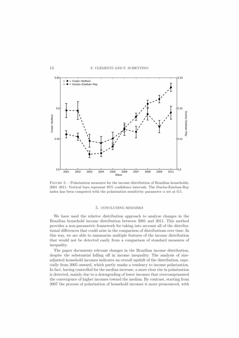
be removed for the relative polarization indices to be computed, we proceedby first estimating “growth-neutral” counter-factual distributions, i.e. what thedistribution of income among households in any one year would have been if themedian had remained a the level of the 2001 reference year; then, for each yearin the period subject to analysis, we compute the values of the aforementionedindices using the estimated counter-factual. In this way, we are sure that theyearly comparisons of polarization levels are only affected by changes in theshape of the distribution and not also by the growth process occurred over thesame study period.15 Figure 3 shows visually the polarization estimates based onthe Foster-Wolfson and the Duclos-Esteban-Ray indices, alongside with the 95%confidence intervals represented by vertical bars.16 The two indices have nearlythe same temporal profile, even if the Duclos-Esteban-Ray index is less stable.As shown by the vertical bars, both measures decline significantly between 2002and 2003. Thereafter, the Foster-Wolfson index rises continuously, and the rise isalmost always statistically significant. The Duclos-Esteban-Ray index tracks theFoster-Wolfson pretty closely over the period of rising polarization, even thoughthe pairwise comparisons indicate that the change is now statistically significantonly between 2007 and 2008 and from 2009 to 2011. The results seem thereforeto portray similar tendencies as that depicted by polarization evaluated usingmeasures based on the relative distribution.17

In sum, rather being solely a story of declining inequality, the recent changesin Brazil’s income distribution bring about a story of polarization. In fact, we areable to document a downgrading trend around the mid-2000s and, by 2007, theemergence of a more marked pattern of polarization. The latter, however, is notsymmetric, as the LRP index is always more positive than the URP, indicatingmore polarization in the lower than in the upper tail.

15Both the Foster-Wolfson and the Duclos-Esteban-Ray measures are relative indices of po-larization, meaning that they remain invariant under equiproportionate changes in all incomes.Therefore, unless the growth process is distribution-neutral—i.e. all levels of income grow atthe same rate, when using such measures the contribution of growth to the estimated level ofincome polarization might more than offset the contribution that is attributable to changingdistribution, which is of major concern here. That is why we have decided to proceed theway we did. See e.g. Ravallion (2010) for a similar approach to the measurement of incomepolarization.

16The Foster-Wolfson and the Duclos-Esteban-Ray measures, as well as their confidenceintervals, have been estimated using the latest version of DASP, the Distributive Analysis StataPackage (Araar and Duclos, 2013), which is freely available at http://dasp.ecn.ulaval.ca/.

17While not shown here due to space constraints, the above-mentioned indices have alsobeen calculated using the relative median-adjusted data, defined in terms of the comparisondistribution in each successive year relative to the 2001 reference distribution, where the latterhas been location-adjusted so as to make the medians of the comparison and reference dis-tributions coincide—in short, the same data used to obtain the relative polarization indices.Once more, after initially experiencing a small (though significant) convergence in householdincomes during the initial years, a marked polarizing trend emerges by the mid-2000s, and thistrend climbs consistently and significantly to the end of the period under study.

14 F. CLEMENTI AND F. SCHETTINO

0.5

0.55

0.6

0.65

Fos

ter−

Wol

fson

2001 2002 2003 2004 2005 2006 2007 2008 2009 20110.3

0.31

0.32

0.33

Wave

Duclos−

Esteban−

Ray

Foster−WolfsonDuclos−Esteban−Ray

Figure 3.—Polarization measures for the income distribution of Brazilian households,2001–2011. Vertical bars represent 95% confidence intervals. The Duclos-Esteban-Rayindex has been computed with the polarization sensitivity parameter α set at 0.5.

5. CONCLUDING REMARKS

We have used the relative distribution approach to analyze changes in theBrazilian household income distribution between 2001 and 2011. This methodprovides a non-parametric framework for taking into account all of the distribu-tional differences that could arise in the comparison of distributions over time. Inthis way, we are able to summarize multiple features of the income distributionthat would not be detected easily from a comparison of standard measures ofinequality.

The paper documents relevant changes in the Brazilian income distribution,despite the substantial falling off in income inequality. The analysis of size-adjusted household incomes indicates an overall upshift of the distribution, espe-cially from 2005 onward, which partly masks a tendency to income polarization.In fact, having controlled for the median increase, a more clear rise in polarizationis detected, mainly due to a downgrading of lower incomes that overcompensatedthe convergence of higher incomes toward the median. By contrast, starting from2007 the process of polarization of household incomes is more pronounced, with

INCOME POLARIZATION IN BRAZIL 15

both the lower and upper tails shifting away from the median of the distribution.

Overall, these findings suggest that the recent improvements in Brazil’s incomedistribution have been propelled mainly by the overall economic growth of thecountry, while social policy programs would have played a key role in affecting theshape of the distribution—leading to a greater polarization at both the top andbottom tails of the income distribution. The observed movements of householdstoward low and high incomes (and away from the middle) could be justified, onthe one side, by deductions and exemptions on taxes that are granted as politicalprivileges to landowners (rents) and financial capitalists (profits), and, on theother side, by the heavy reliance on indirect taxation that disproportionatelyburden the income of poor and middle-income households, who consequentlybear a significant share of the total cost for social programs (e.g. Birdsall et al.,2008, ch. 4.).

Hence, sustaining reductions in both inequality and poverty by making themless growth-dependent represents a key challenge for Brazil going forward: asborne out by our results, under a scenario of poor performance growth the shapeeffect would be brought to prevail, thereby generating a more unequal society.Considering the recent halt in Brazil’s economic growth that followed the globaleconomic crisis, this paper suggests adopting policies well targeted to a “real”re-distribution of resources, i.e. aimed at allowing structural improvements in theincome distribution that go beyond the effects of economic growth. Among these,making the tax system somewhat more progressive by increasing the tax burdenon the income of rich households (including business profits as well as financialand agricultural rents) would improve the overall distribution of income and,at the same time, free up precious resources for domestic demand (especiallyby the middle class). Furthermore, reform programs to alleviate the unequaldistribution of land would grant to poorest households—in particular those livingin the North and Northeast regions of Brazil—the necessary tools to get outof extreme poverty and consequently reduce their actual dependence on socialtransfers.18

The paper can be extended in several directions. Perhaps the most obviousextension is to examine how different sources of household income might haveimpacted the observed increase of income polarization. Also, the decompositionof the relative distribution according to covariates measured on households wouldallow one to detect the contribution of different household characteristics suchas geographic location, gender, age and ethnicity to the observed changes. Dueto the richness of data available from the PNAD and the many opportunities

18Brazil has one of the most unequal distribution of land in the world. The concentrationof property in Brazil is so skewed that the largest 3.5% of landholdings represent 56% of totalagricultural land (Hidalgo et al., 2010). The Gini coefficient of land inequality remained stablebetween 1967 and 1998, measuring around 0.84 in both the beginning and end of the period(Hoffmann, 1998). Since then, it increased to 0.856 in 1995 and 0.872 in 2006 (IBGE, 1997,2009). Some regional differences exist, but land inequality in all regions is high when comparedinternationally (Hoffmann and Ney, 2010).

16 F. CLEMENTI AND F. SCHETTINO

offered by the relative distribution approach, we are in a good position to readilyexpand our analysis in the near future.

REFERENCES

Alderson, A. S., J. Beckfield, and F. Nielsen (2005): “Exactly How Has Income InequalityChanged? Patterns of Distributional Change in Core Societies,” International Journal of

Comparative Sociology, 46, 405–423.Alderson, A. S. and K. Doran (2011): “Global Inequality, Within-Nation Inequality, and

the Changing Distribution of Income in Seven Transitional and Middle-Income Societies,”in Inequality Beyond Globalization: Economic Changes, Social Transformations, and the

Dynamics of Inequality, ed. by C. Suter, New Brunswick, NJ: Transaction Publishers, 183–200.

——— (2013): “How Has Income Inequality Grown? The Reshaping of the Income Distributionin LIS Countries,” in Income Inequality: Economic Disparities and the Middle Class in

Affluent Countries, ed. by J. C. Gornick and M. Jantti, Stanford, CA: Stanford UniversityPress, 51–74.

Anderson, G., O. Linton, and T. W. Leo (2012): “A Polarization-Cohesion Perspective onCross-Country Convergence,” Journal of Economic Growth, 17, 49–69.

Araar, A. and J.-Y. Duclos (2013): User Manual for Stata Package DASP: Version 2.3,PEP, World Bank, UNDP and Universite Laval, available at http://dasp.ecn.ulaval.ca/modules/DASP_V2.3/DASP_MANUAL_V2.3.pdf.

Atkinson, A. B., L. Rainwater, and T. M. Smeeding (1995): Income Distribution in OECD

Countries: Evidence from Luxembourg Income Study, Paris: Organization for Economic Co-operation and Development.

Barros, R. P. (2007): “A Efetividade do Salario Mınimo em Comparacao a do Programa BolsaFamılia como Instrumento de reducao da Pobreza e da Desigualdade,” in Desigualdade de

Renda no Brasil: Uma Analise da Queda Recente, ed. by R. P. Barros, M. N. Foguel, andG. Ulyssea, Brasılia, DF: Instituto de Pesquisa Economica Aplicada (IPEA), vol. 2, 507–549.

Barros, R. P., M. De Carvalho, S. Franco, and R. Mendonca (2010): “Markets, theState, and the Dynamics of Inequality in Brazil,” in Declining Inequality in Latin America:

A Decade of Progress?, ed. by L. F. Lopez-Calva and N. Lustig, Washington, DC: BrookingsInstitution Press and UNDP, 134–174.

Bianchi, M. (1997): “Testing for Convergence: Evidence from Nonparametric MultimodalityTests,” Journal of Applied Econometrics, 12, 393–409.

Birdsall, N., A. De La Torre, and A. Menezes (2008): Fair Growth: Economic Policies

for Latin America’s Poor and Middle-Income Majority, Washington, DC: Center for GlobalDevelopment.

Borraz, F., N. G. Pampillon, and M. Rossi (2011): “Polarization and the Middle Class,”dECON Working Paper 20, Universidad de la Republica, Montevideo, available at http://www.fcs.edu.uy/archivos/2011.pdf.

Bourguignon, F. (2003): “The Growth Elasticity of Poverty Reduction: Explaining Hetero-geneity across Countries and Time Periods,” in Inequality and Growth: Theory and Policy

Implications, ed. by T. S. Eicher and S. J. Turnovsky, Cambridge, MA: The MIT Press,3–26.

——— (2004): “The Poverty-Growth-Inequality Triangle,” Working Paper 125, Indian Councilfor Research on International Economic Relations, New Delhi, available at http://www.

icrier.org/pdf/wp125.pdf.Centre for Economics and Business Research (2011): “World Economic

League Table,” Technical report, Centre for Economics and Business Re-search, London, available at http://www.cebr.com/wp-content/uploads/

Cebr-World-Economic-League-Table-press-release-26-December-2011.pdf.Chakravarty, S. R. (2009): Inequality, Polarization and Poverty: Advances in Distributional

Analysis, New York, NY: Springer-Verlag Inc.

INCOME POLARIZATION IN BRAZIL 17

Chakravarty, S. R. and C. D’Ambrosio (2010): “Polarization Orderings of Income Distri-butions,” Review of Income and Wealth, 56, 47–64.

Chakravarty, S. R. and A. Majumder (2001): “Inequality, Polarization and Welfare: Theoryand Applications,” Australian Economic Papers, 40, 1–13.

Chakravarty, S. R., A. Majumder, and S. Roy (2007): “A Treatment of Absolute Indicesof Polarization,” Japanese Economic Review, 58, 273–293.

Coggiola, O. (2010): “Fome, Capitalismo, e Programas Sociais Compensatorios,” mimeo.Conti, P. L., M. G. Pittau, and R. Zelli (2006): “Metodi non parametrici nell’analisi della

distribuzione del reddito: problemi empirici ed aspetti metodologici,” Rivista di Politica

Economica, 96, 195–242.Cowell, F. A., S. P. Jenkins, and J. A. Litchfield (1996): “The Changing Shape of the

UK Income Distribution: Kernel Density Estimates,” in New Equalities: The Changing

Distribution of Income and Wealth in the United Kingdom, ed. by J. Hills, Cambridge, UK:Cambridge University Press, 49–75.

D’Ambrosio, C. (2001): “Household Characteristics and the Distribution of Income in Italy:An Application of Social Distance Measures,” Review of Income and Wealth, 47, 43–64.

Duclos, J.-Y., J.-M. Esteban, and D. Ray (2004): “Polarization: Concepts, Measurement,Estimation,” Econometrica, 72, 1737–1772.

Esteban, J.-M., C. Gradın, and D. Ray (2007): “An Extension of a Measure of Polariza-tion, with an Application to the Income Distribution of Five OECD Countries,” Journal of

Economic Inequality, 5, 1–19.Esteban, J.-M. and D. Ray (1994): “On the Measurement of Polarization,” Econometrica,

62, 819–851.——— (1999): “Conflict and Distribution,” Journal of Economic Theory, 87, 379–415.——— (2011): “Linking Conflict to Inequality and Polarization,” The American Economic

Review, 101, 1345–1374.Fiszbein, A., N. Schady, F. H. G. Ferreira, M. Grosh, N. Keleher, P. Olinto, and

E. Skoufias (2009): Conditional Cash Transfers: Reducing Present and Future Poverty,Washington, DC: World Bank.

Foster, J. E. and M. C. Wolfson (1992): “Polarization and the Decline of the Middle Class:Canada and the US,” OPHI Working Paper 31, University of Oxford, Oxford, availableat http://www.ophi.org.uk/working-paper-number-31/, now in Journal of Economic In-equality 8, 247–273, 2010.

Gasparini, L. and N. Lustig (2011): “The Rise and Fall of Income Inequality in Latin Amer-ica,” in The Oxford Handbook of Latin American Economics, ed. by J. A. Ocampo andJ. Ros, New York, NY: Oxford University Press, 691–714.

Gigliarano, C. and K. Mosler (2009): “Constructing Indices of Multivariate Polarization,”Journal of Economic Inequality, 7, 435–460.

Gradın, C. (2000): “Polarization by Sub-Populations in Spain, 1973–91,” Review of Income

and Wealth, 46, 457–474.Hall, A. (2006): “From Fome Zero to Bolsa Famılia: Social Policies and Poverty Alleviation

under Lula,” Journal of Latin American Studies, 38, 689–709.Handcock, M. S. (2011): Relative Distribution Methods, Los Angeles, CA, version 1.6. Project

home page at http://www.stat.ucla.edu/~handcock/RelDist.Handcock, M. S. and M. Morris (1998): “Relative Distribution Methods,” Sociological

Methodology, 28, 53–97.——— (1999): Relative Distribution Methods in the Social Sciences, New York, NY: Springer-

Verlag Inc.Hao, L. and D. Q. Naiman (2010): Assessing Inequality, Thousand Oaks, CA: SAGE Publi-

cations, Inc.Henderson, D. J., C. Parmeter, and R. R. Russell (2008): “Modes, Weighted Modes,

and Calibrated Modes: Evidence of Clustering Using Modality Tests,” Journal of Applied

Econometrics, 23, 607–638.Hidalgo, F. D., S. Naidu, S. Nichter, and N. Richardson (2010): “Economic Determinants

of Land Invasions,” The Review of Economics and Statistics, 92, 505–523.

18 F. CLEMENTI AND F. SCHETTINO

Higgins, S. (2012): “The Impact of Bolsa Famılia on Poverty: Does Brazil’s Conditional CashCransfer Program Have a Rural Bias?” Journal of Politics & Society, 23, 88–125.

Hoffmann, R. (1998): “A Estrutura Fundıaria no Brasil de Acordo com o Cadastro do INCRA:1967 a 1998,” Technical report, Ministerio do Desenvolvimento Agrario, Brasılia, DF.

Hoffmann, R. and M. G. Ney (2010): “Estrutura Fundiaria e Propriedade Agrıcola no Brasil,Grandes Regioes e Unidades da Federacao (de 1970 a 2008),” Technical report, Ministeriodo Desenvolvimento Agrario, Brasılia, DF, available at http://www.nead.gov.br/portal/

nead/publicacoes/download_orig_file?pageflip_id=8632224.Holzmann, H., S. Vollmer, and J. Weisbrod (2007): “Twin Peaks or Three Components?

Analyzing the World’s Cross-Country Distribution of Income,” IAI Discussion Paper 162,University of Gottingen, Gottingen, available at http://www2.vwl.wiso.uni-goettingen.

de/ibero/papers/DB162.pdf.Instituto Brasileiro de Geografia e Estatıstica (1997): “Censo Agropecuario de 1995–

1996,” Technical report, Instituto Brasileiro de Geografia e Estatıstica (IBGE), Riode Janeiro, RJ, available at http://www.ibge.gov.br/english/estatistica/economia/

agropecuaria/censoagro/1995_1996/default.shtm.——— (2009): “Censo Agropecuario 2006. Brasil, Grandes Regioes e Unidades da Federacao,”

Technical report, Instituto Brasileiro de Geografia e Estatıstica (IBGE), Rio de Janeiro,RJ, available at http://www.ibge.gov.br/english/estatistica/economia/agropecuaria/

censoagro/default.shtm.Jenkins, S. P. (1995): “Did the Middle Class Shrink During the 1980s? UK Evidence From

Kernel Density Estimates,” Economic Letters, 49, 407–413.——— (1996): “Recent Trends in the UK Income Distribution: What Happened and Why?”

Oxford Review of Economic Policy, 12, 29–46.Jenkins, S. P. and P. Van Kerm (2005): “Accounting for Income Distribution Trends: A

Density Function Decomposition Approach,” Journal of Economic Inequality, 3, 43–61.Johnson, P. A. (2000): “A Nonparametric Analysis of Income Convergence Across the US

States,” Economics Letters, 69, 219–223.Jones, C. I. (1997): “On the Evolution of the World Income Distribution,” Journal of Eco-

nomic Perspectives, 11, 19–36.Kakwani, N. (1993): “Poverty and Economic Growth with Application to Cote d’Ivoire,”

Review of Income and Wealth, 39, 121–139.Lasso de la Vega, M. C., A. Urrutia, and H. Dıez (2010): “Unit Consistency and Bipo-

larization of Income Distributions,” Review of Income and Wealth, 56, 65–83.Lasso de la Vega, M. C. and A. M. Urrutia (2006): “An Alternative Formulation of

Esteban-Gradın-Ray Extended Measure of Polarization,” Journal of Income Distribution,15, 42–54.

Levy, F. and R. J. Murnane (1992): “U.S. Earnings Levels and Earnings Inequality: AReview of Recent Trends and Proposed Explanations,” Journal of Economic Literature, 30,1333–1381.

Lindert, K., A. Linder, J. Hobbs, and B. de la Briere (2007): “The Nuts andBolts of Brazil’s Bolsa Famılia Program: Implementing Conditional Cash Transfers ina Decentralized Context,” Social protection discussion paper no. 0709, World Bank,Washington, DC, available at http://siteresources.worldbank.org/SOCIALPROTECTION/

Resources/SP-Discussion-papers/Safety-Nets-DP/0709.pdf.Lopez-Calva, L. F. (2012): “Declining Income Inequality in Brazil: The Proud Outlier,” World

Bank – Inequality in Focus, 1, 5–8.Lopez-Calva, L. F. and S. Rocha (2012): “Exiting Belindia? Lesson From the Re-

cent Decline in Income Inequality in Brazil,” Report no. 70155, World Bank, Washing-ton, DC, available at http://documents.worldbank.org/curated/en/2012/01/16423641/

exiting-belindia-lesson-recent-decline-income-inequality-brazil.Massari, R. (2009): “Is Income Becoming More Polarized in Italy? A Closer Look With a Dis-

tributional Approach,” DSE Working Paper 1, Sapienza University of Rome, Rome, availableat http://phdschool-economics.dse.uniroma1.it/website/WorkingPapers/MassariWP1.

pdf.

INCOME POLARIZATION IN BRAZIL 19

Massari, R., M. G. Pittau, and R. Zelli (2009a): “A Dwindling Middle Class? ItalianEvidence in the 2000s,” Journal of Economic Inequality, 7, 333–350.

——— (2009b): “Caos calmo: l’evoluzione dei redditi familiari in Italia,” in L’Italia delle

disuguaglianze, ed. by L. Cappellari, P. Naticchioni, and S. Staffolani, Rome: Carocci editore,19–28.

Milanovic, B. (2000): “A New Polarization Measure and Some Applications,” mimeo, availableat http://siteresources.worldbank.org/INTDECINEQ/Resources/polariz.pdf.

Morris, M., A. D. Bernhardt, and M. S. Handcock (1994): “Economic Inequality: NewMethods for New Trends,” American Sociological Review, 59, 205–219.

Organization for Economic Co-operation and Development (2011): Divided We Stand:

Why Inequality Keeps Rising, Paris: OECD Publishing.Paap, R. and H. K. van Dijk (1998): “Distribution and Mobility of Wealth of Nations,”

European Economic Review, 42, 1269–1293.Pittau, M. G. and R. Zelli (2001): “Income Distribution in Italy: A Nonparametric Analysis,”

Statistical Methods and Applications, 10, 175–189.——— (2004): “Testing for Changing Shapes of Income Distribution: Italian Evidence in the

1990s From Kernel Density Estimates,” Empirical Economics, 29, 415–430.——— (2006): “Trends in Income Distribution in Italy: A Non-Parametric and a Semi-

Parametric Analysis,” Journal of Income Distribution, 15, 90–118.Pittau, M. G., R. Zelli, and P. A. Johnson (2010): “Mixture Models, Convergence Clubs

and Polarization,” Review of Income and Wealth, 56, 102–122.Poggi, A. and J. Silber (2010): “On Polarization and Mobility: A Look at Polarization in

the Wage-Career Profile in Italy,” Review of Income and Wealth, 56, 123–140.Pressman, S. (2007): “The Decline of the Middle Class: An International Perspective,” Journal

of Economic Issues, 41, 181–200.Quah, D. T. (1996a): “Convergence Empirics Across Economies with (Some) Capital Mobil-

ity,” Journal of Economic Growth, 1, 95–124.——— (1996b): “Twin Peaks: Growth and Convergence in Models of Distribution Dynamics,”

The Economic Journal, 106, 1045–1055.——— (1997): “Empirics for Growth and Distribution: Stratification, Polarization, and Con-

vergence Clubs,” Journal of Economic Growth, 2, 27–59.Ravallion, M. (2010): “The Developing World’s Bulging (but Vulnerable) Middle Class,”

World Development, 38, 445–454.Reynal-Querol, M. (2002): “Ethnicity, Political Systems and Civil War,” Journal of Conflict

Resolution, 46, 29–54.Robinson, J. A. (2010): “The Political Economy of Redistributive Policies,” in Declining

Inequality in Latin America: A Decade of Progress?, ed. by L. F. Lopez-Calva and N. Lustig,Washington, DC: Brookings Institution Press and UNDP, 39–71.

Rodrıguez, J. G. and R. Salas (2003): “Extended Bi-Polarization and Inequality Measures,”Research on Economic Inequality, 9, 69–83.

Silber, J. and J. Deutsch (2012): “On Bi-Polarization and the Middle Class in Latin America:A Look at the First Decade of the Twenty First Century,” paper presented at the 32nd Gen-eral Conference of the International Association for Research in Income and Wealth, Boston,US, August 5–11, 2012, available at http://www.iariw.org/papers/2012/SilberPaper.pdf.

Silber, J., M. Hanoka, and J. Deutsch (2007): “On the Link Between the Concepts ofKurtosis and Bipolarization,” Economics Bulletin, 4, 1–6.

Soares, S. S. D. (2012): “Bolsa Famılia, its Design, its Impacts and Possibilities for theFurture,” Working paper no. 89, UNDP – International Policy Centre for Inclusive Growth(IPC-IG), Brasilia, DF, available at http://www.ipc-undp.org/pub/IPCWorkingPaper89.

pdf.Van Kerm, P. (2003): “Adaptive Kernel Density Estimation,” The Stata Journal, 3, 148–156.Wang, Y.-Q. and K.-Y. Tsui (2000): “Polarization Orderings and New Classes of Polarization

Indices,” Journal of Public Economic Theory, 2, 349–363.Wolfson, M. C. (1994): “When Inequalities Diverge,” The American Economic Review, 84,

353–358.

20 F. CLEMENTI AND F. SCHETTINO

——— (1997): “Divergent Inequalities: Theory and Empirical Results,” Review of Income and

Wealth, 43, 401–421.World Bank (2004): Inequality and Economic Development in Brazil, Washington, DC: World

Bank.Zhang, X. and R. Kanbur (2001): “What Difference Do Polarisation Measures Make? An

Application to China,” Journal of Development Studies, 37, 85–98.