Including the Effect of a Future Test and Redesignin Reliability Calculations

Diane Villanueva,∗ Raphael T. Haftka,† and Bhavani V. Sankar‡

University of Florida, Gainesville, Florida 32611

DOI: 10.2514/1.J051150

It is common to test components after they are designed and redesign if necessary. The reduction of the uncertainty

in the probability of failure that can occur after a test is usually not incorporated in reliability calculations at the

design stage. This reduction in uncertainty is accomplished by additional knowledge provided by the test and by

redesign when the test reveals that the component is unsafe or overly conservative. In this paper, a methodology is

developed to estimate the effect of a single future thermal test followed by redesign and to model the effect of the

resulting reduction of the uncertainty in the probability of failure. Using assumed distributions of computation and

experimental errors and given redesign rules, possible outcomes of the future test and redesign throughMonte Carlo

sampling are obtained to determinewhat changes in probability of failure, design, andweight will occur. In addition,

Bayesian updating is used to gain accurate estimates of the probability of failure after a test. These methods are

demonstrated through a future thermal test on an integrated thermal protection system. Performing redesign

following a single future test can reduce the probability of failure by orders of magnitude, on average, when the

objective of the redesign is to restore original safety margins. Redesign for a given reduced probability of failure

allows additional weight reduction.

Nomenclature

C = capacityDL = lower bound for deterministic redesign criterionDU = upper bound for deterministic redesign criteriond = design variableds = foam thickness, mec = computational erroreextrap = extrapolation errorex = experimental errorf�T� = probability distribution of the temperatureg = limit state functionI = indicator functionltest�T� = likelihood function of obtaining the test-article

temperatureM = number of samples of the capacitym = mass per unit area, kg=m2

N = number of samples of the responsePL = lower bound for probabilistic redesign criterionPU = upper bound for probabilistic redesign criterionpf;analyst = analyst-estimated probability of failure, %pf;target = probabilistic redesign probability of failure target, %pf;true = true probability of failure, %R = responser = random variableT = temperature, K�dlim = limit of distance between test design and other

design

Subscripts

allow = allowableBayes = value obtained from Bayesian updatingcalc = calculatedcorr = correctedini = initialinp = inputmeas = measuredtest = test articletrue = truePtrue = possible true

Superscript

upd = updated

I. Introduction

I N RELIABILITY-BASED design optimization, uncertainties areconsidered when calculating the reliability of the structure. In the

design process, uncertainty is often compensated for with safetyfactors and knockdown factors. However, after design, it is cus-tomary for the component to undergo various uncertainty-reductionmeasures (URMs). Examples of URMs in the aerospacefield includethermal and structural testing, inspection, health monitoring,maintenance, and improved analysis and failure modeling. Sincemost components undergo these URMs, it would be beneficial toinclude their effects in the design process.

In recent years, there has been amovement to quantify the effect ofURMs on the safety of the product over its life cycle. Much work hasbeen completed in the areas of inspection and maintenance forstructures under fatigue loading. Fujimoto et al. [1], Toyoda-Makino[2], and Garbatov and Soares [3] developed methods to optimizeinspection schedules for a given structural design to maintain aspecific level of reliability. Even further, Kale et al. [4,5] exploredhow simultaneous design of the structure and inspection scheduleallows the trading of cost of additional structural weight againstinspection cost of stiffened panels affected by fatigue crack growth.

However, there are few studies that have incorporated the effects offuture tests followed by possible redesign on the design of a structure.Studies by Acar et al. [6,7] investigated the effects of future tests andredesign on the final distribution of failure stress and structuraldesign with varying numbers of tests at the coupon, element, and

Presented at the 12th AIAA Non-Deterministic Approaches Conference,Orlando, FL, 12–15 April 2010; received 30 December 2010; revisionreceived 20 March 2011; accepted for publication 8 May 2011. Copyright ©2011 by Diane Villanueva, Raphael T. Haftka, and Bhavani V. Sankar.Published by the American Institute of Aeronautics and Astronautics, Inc.,with permission. Copies of this paper may be made for personal or internaluse, on condition that the copier pay the $10.00 per-copy fee to the CopyrightClearance Center, Inc., 222 Rosewood Drive, Danvers, MA 01923; includethe code 0001-1452/11 and $10.00 in correspondence with the CCC.

∗Graduate Research Assistant, Department of Mechanical and AerospaceEngineering. Student Member AIAA.

†Distinguished Professor, Department of Mechanical and AerospaceEngineering. Fellow AIAA.

‡Ebaugh Professor and University of Florida Research FoundationProfessor, Department of Mechanical and Aerospace Engineering. AssociateFellow AIAA.

AIAA JOURNALVol. 49, No. 12, December 2011

2760

certification levels. Such studies showed that these tests with possibleredesign can greatly reduce the probability of failure, and theyestimated the required structural weight to achieve the samereduction without tests.

In this study, we examine the effect of a single future thermal testfollowed by possible redesign on the reliability and weight of anintegrated thermal protection system (ITPS). An integrated thermalprotection system protects space vehicles from the severe aero-dynamic heating experienced upon atmospheric reentry while alsoproviding some structural load bearing benefit. The thermal testconsidered in this study measures the maximum temperature of thebottom face sheet, which is critical due to its proximity to theunderlying vehicle structure. A design is considered to have failedthermally if it exceeds the maximum allowable temperature.

In previous work on the optimization of the ITPS, Villanueva et al.[8] used probability of failure calculations that considered only thevariability in geometric and material parameters and error due toshortcomings in the analytical model. Expanding on those studies,we include the information gained from a test in a temperatureestimate, the reduction in uncertainty resulting from the test, and theability of the test to guide redesign for dangerous or overlyconservative designs. Thereby, the objectives of this paper are asfollows:

1) Present amethodology to both predict and include the effect of afuture redesign following a test during the design stage.

2) Illustrate the ability of a test in combination with redesign toreduce the probability of failure even when a test shows that thedesign is computationally unconservative.

3) Examine the overall changes in mass resulting from redesignbased on the future test.

A description of the ITPS is presented in Sec. II. Next, theuncertainty model and probability of failure calculations aredescribed in Sec. III. Section IV continues with the methodology tocalibrate the computational model based on a test and includesredesign based on the test. The method to simulate future tests issummarized in Sec. V. Section VI presents an illustrative examplethat details the effect of including the test and redesign in probabilityof failure calculations. The paper then concludeswith a summary andideas for future work in Sec. VII.

II. ITPS Description

Figure 1 shows the ITPS panel being studied, which is acorrugated-core sandwich-panel concept. The design consists of atop face sheet and webs made of titanium alloy (Ti-6Al-4V) and abottom face sheet made of beryllium. Saffil® foam is used asinsulation between thewebs. The relevant geometric variables of theITPS design are also shown on the unit cell in Fig. 1. These variablesare the top face thickness tT , bottom face thickness tB, thickness ofthe foam dS, web thickness tw, corrugation angle �, and length of unitcell 2p.

Thermal analysis of the ITPS is done using 1-D heat transferequations on amodel of the unit cell. The heat flux incident on the topface sheet of the panel is highly dependent on the vehicle shape aswell as the vehicle’s trajectory. As in previous studies by Bapanapalli[9], incident heat flux on a Space Shuttle-like vehicle was used. A

large portion of the heat is radiated out to the ambient by the top facesheet, and the remaining portion is conducted into the ITPS. Weconsider theworst-case scenario, where the bottom face sheet cannotdissipate heat, by assuming that the bottom face sheet is perfectlyinsulated. Also, there is no lateral heat flow out of the unit cell, so thatheat flux on the unit cell is absorbed by that unit cell only. For a morein-depth description of the model and boundary conditions, thereader is referred to the Bapanapalli reference.

The maximum temperature of the bottom face sheet of the ITPSpanel is calculated using the quadratic response surface developed byVillanueva et al. [8] by a process similar to that of Gogu et al. [10],using the MATLAB toolbox developed by Viana.§ It is a function ofthe previously described geometric variables and the density, thermalconductivity, and specific heat of titanium alloy, beryllium, andSaffil® foam. The mass per unit area m of the ITPS is calculatedusing Eq. (1), where �T , �B, and �w are the densities of the materialsthat make up the top face sheet, bottom face sheet, and web,respectively:

m� �TtT � �BtB ��wtwdSp sin �

(1)

An experiment that finds the bottom face sheet temperature of asmall ITPS panel is usually conducted in a vacuum chamber withheat applied to the top face sheet by heat lamps. The sides of the panelare typically surrounded by some kind of insulation to prevent lateralheat loss. The temperature of the bottom face sheet is found withthermocouples embedded into or in contact with the lower surface ofthe bottom face sheet.

III. Uncertainty Modeling

A. Classification of Uncertainties

Oberkampf et al. [11] provided an analysis of different sources ofuncertainty in engineering modeling and simulation, which wassimplified by Acar et al. [6]. We use a similar classification tocategorize types of uncertainty as errors (uncertainties that applyequally to every ITPS) or variability (uncertainties that vary in eachindividual ITPS). We further describe errors as mostly epistemic andvariability as aleatory. It is important to distinguish between types ofuncertainty because a specific uncertainty-reduction measure maytarget either error or variability. Tests reduce errors by allowing us tocalibrate analytical models. For example, testing can be done toreduce the uncertainty in failure predictions due to high stresses.Variability can be reduced by lowering tolerances in manufacturing.Variability is modeled as random uncertainties that can be modeledprobabilistically. In contrast, errors are fixed for a given ITPS and arelargely unknown, but here they aremodeled probabilistically as well.

Variability in material properties and construction of the ITPSleads to variability in the ITPS thermal response. More specifically,wewill have variability in the calculated temperature, due to the inputvariabilities.We simulate this process with aMonte Carlo simulationthat generates values of the random variables r based on an estimateddistribution and calculates the bottom face sheet temperatureTcalc for

Fig. 1 Corrugated-core sandwich-panel ITPS concept.

§Data available online at http://sites.google.com/site/felipeacviana/.

VILLANUEVA, HAFTKA, AND SANKAR 2761

each, generating the probability distribution function. The calculatedtemperature distribution that reflects the random variability isdenoted fcalc�T�. In estimating the probability of failure, we alsoneed to account for the modeling or computational error. We denotethis computational error by ec, where ec is modeled as a uniformlydistributed random variable within confidence limits the in thecomputationalmodel as defined by the analyst. Unlike thevariability,the error has a single value, and the uncertainty is due to our lack ofknowledge.

For a given design given by d and r, the possible true temperatureTPtrue can be found by Eq. (2) in terms of possible computationalerrors ec. The sign in front of ec is negative, so a positive error impliesa conservative calculation, meaning that it overestimates thetemperature:

TPtrue�d; r; ec� � Tcalc�d; r��1 � ec� (2)

Since the analyst does not know ec and it is modeled as a randomvariable, we can form a distribution of the possible true temperature,denoted as fPtrue�T�. To illustrate the difference between the truedistribution of the temperature ftrue�T� and possible true distributionfPtrue�T�, let us consider a simple example where the calculatedtemperature of the nominal design is 1, the true temperature is 1.05,and the computational error is uniformly distributed in the range[�0:1, 0.1]. The possible true temperature without variability areuniformly distributed in the range [0.9, 1.1] by Eq. (2). Now, let usconsider an additional variability in the temperature due tomanufacturing tolerances in the range [�0:02, 0.01], such thatTcalc�d; r� is uniformly distributed in the range [0.98, 1.01]. Finally,the true temperature will vary from [1.03, 1.06] as ftrue�T�, and thepossible true temperature will vary from [0.882, 1.111] as fPtrue�T�.

Figure 2 illustrates howwe arrive at the distribution fPtrue�T�. Theinput random variables have initial distributions, denoted as finp�r�,and these random variables, in combination with the designvariables, lead to the distribution of the calculated temperaturefcalc�T�. The random computational error is applied, leading to thedistribution of the possible true temperature fPtrue�T�, which has awider distribution than fcalc�T�.

As previously noted, ec is modeled as a random variable notbecause it is random, but because its value is unknown to the analyst.To emphasize this point, the actual true temperature is known onlywhen we know the actual value of ec as ec;true as illustrated in Eq. (3)below:

Ttrue�d; r� � Tcalc�d; r��1 � ec;true� (3)

Again, these true values are unknown to the analyst. Thisdistinction between true values and analyst-estimated, possible truevalues is important and will be a point of comparison throughout thispaper.

Figure 3 shows an example of the probability distribution of thetrue temperature ftrue�T�, as well as the probability density functions(PDFs) of fcalc�T� and fPtrue�T�. For this example, we modeled thevariability in the material properties and variability in geometry withnormal distributions, and we modeled the computational error with auniform distribution. The plots of each PDF show the probability ofexceeding the allowable temperature Tallow, represented by the areawhere the temperature exceeds the allowable.

We chose an illustration where the computational error isunconservative so the fcalc�T� provides an underestimate of the

probability of failure given by ftrue�T�. This computational errorbetween the mean of fcalc�T� and the mean of ftrue�T� is ec;true.However, since we include ec as a random variable, we widened thedistribution fcalc�T�, resulting in fPtrue�T�. This provides a moreconservative estimate of the probability that can compensate for theunconservative calculation. Of course, when the error in thecalculation is conservative, this wide distribution will grosslyoverestimate the probability of failure.

B. True Probability of Failure Calculation

The true probability of failure of a design dwith random variablesr can be found when the true computational error is known. This isclearly a hypothetical situation because in reality the true compu-tational error is not known by the analyst. Here, Monte Carlosimulation is used to calculate the true probability of failure. Thelimit state equation g is formulated as the difference between acapacity C and response R as shown in Eq. (4):

g� Tallow � Ttrue�d; r� � C � R (4)

Sincewe consider failure to occurwhen themaximumbottom facesheet temperature exceeds the allowable temperature Tallow, theresponse is Ttrue and the capacity is the allowable temperature. Thetrue probability of failure pf;true is estimated with Eq. (5):

pf;true �1

N

XNi�1

I�g�Ci; Ri� � 0 (5)

The indicator function I equals 1 if the response exceeds the capacity,and it equals 0 for the opposite case. The number of samples is N.

C. Analyst-Estimated Probability of Failure Calculation

Since the true computational error is unknown, the true probabilityof failure is unknown as well. Because of this, the best estimate theanalyst can obtain uses the calculated temperature Tcalc and thecomputational error through the possible true temperature of Eq. (2)to determine the estimated probability of failure with the limit stateequation formulated as in Eq. (6):

g� Tallow � TPtrue�d; r; ec� � C � R (6)

Since the two types of uncertainty (computational errors andvariability in material properties and geometry) in the response areindependent, separableMonte Carlo sampling [12] can be usedwhenevaluating the probability of failure. The limit state equation can bereformulated so that the computational error is on the capacity side,and all random variables associated with material properties andgeometry lie on the response side:

Fig. 2 Illustration of the variability of the input random variables,

calculated value, computational error, and resulting distribution of

possible true temperature.

Fig. 3 Illustration with unconservative calculation of temperature

when including the error in the estimate improves the estimate of the

probability of failure.

2762 VILLANUEVA, HAFTKA, AND SANKAR

g� Tallow1 � ec

� Tcalc�d; r� � C � R (7)

This analyst-estimated probability of failure pf;analyst can then becalculated with Eq. (8), whereM and N are the number of capacityand response samples, respectively:

pf;analyst �1

MN

XNi�1

XMj�1

I�g�Cj; Ri� � 0 (8)

IV. Including the Effect of a CalibrationTest and Redesign

We consider a test, performed for the purpose of validating andcalibrating a model, for a selected design dtest to determine thetemperature of the test article Ttest. We further assume that the testarticle is carefully measured for both dtest and rtest so that both areaccurately known and that the errors in the computed temperaturesdue to uncertainty in the values of dtest and rtest are small comparedwith the measurement errors and can be neglected. If no errors aremade in the measurements of dtest, rtest, and Ttest, then theexperimental result is actually the true temperature of the test article.We denote this error-free test temperature Ttest;true:

Ttest;true � Ttrue�dtest; rtest� (9)

However, there is unknown measurement error ex, which we modelas a randomvariable based on our estimate of the accuracy of the test.Themeasured temperatureTmeas then includes the experimental errorex;true. The experimental error could also include a component due tothe fact that rtest is not perfectly known:

Tmeas �Ttest;true1 � ex;true

(10)

Using the computational and experimental results, along with thecorresponding error estimates for the test article, we are able to refinethe calculated value and its error for any design described by thedesign variables d and random variables r. In this way, the result ofthe single test can be used to calibrate calculations for other designs.We examine two methods, which take different approaches in usingthe test as calibration. The first approach introduces a simplecorrection factor based on the test result. The second uses theBayesianmethod to update the uncertainty of the calculated value fordtest based on the test result and then transfers this updateduncertainty to other calculations as the means of calibration.

A. Correction-Factor Approach

The correction factor approach is a fairly straightforward methodof calibration. Assuming that the test result is more accurate than thecalculated result for the test article, we scale Tcalc for any value of dand r by the ratio of the test result to the calculated result to obtain thecorrected calculation Tcalc;corr:

Tcalc;corr � Tcalc�d; r��

Tmeas

Tcalc�dtest; rtest�

�(11)

B. Bayesian-Updating Approach

Before the test, we have an expectation of the test results based onthe computational result of dtest and rtest. We denote this distributionbyfinitest;Ptrue, which can beviewed as the distribution offPtrue�T� of thetest article with fixed random variables rtest. Furthermore, it may beviewed as the possible true temperature distribution of the test articlejust before the test.

In the test, we measure a temperature Tmeas. Because ofexperimental error ex, the true test result Ttest;true is not equal to Tmeas

(as seen in Eq. (10)). The possible true value of the test result isinstead given as

Tmeastest;Ptrue � Tmeas�1 � ex� (12)

where Tmeastest;Ptrue forms the distribution of possible true test results

available from the measurements only. We thus have two distrib-utions of possible true test results. One is based on the calculatedvalue and the distribution of the calculation error, and the other isbased on the measurement and the distribution of the measurementerror.

TheBayesian approach combines these two distributions to obtaina narrower andmore informative distribution. In this formulation, theprobability distribution of the possible true temperature of the testarticle ftest;Ptrue�T� is updated as

fupdtest;Ptrue�T� �ltest�T�finitest;Ptrue�T�R�1

�1 ltest�T�finitest;Ptrue�T� dT(13)

where the likelihood function ltest�T� is the conditional probabilitydensity of obtaining the test result Tmeas when the true temperature ofthe test article is T. That is, ltest is the probability density of T=�1 �ex� evaluated at T � Tmeas.

The updated estimate fupdtest;Ptrue�T� is the distribution of the updatedtrue possible test result Tupd

test;Ptrue. This is used to find the distributionof the Bayesian estimate of the computational error eBayes withEq. (14):

eBayes � 1 �Tupdtest;Ptrue

Tcalc�dtest; rtest�(14)

We can then replace the possible true temperature given by Eq. (2)with a true temperature that uses the Bayesian estimate of the error:

TPtrue�d; r; eBayes� � Tcalc�d; r��1 � eBayes��1 � eextrap� (15)

The additional error eextrap is included to account for the error thatoccurs when applying this Bayesian estimate of the error to somedesign other than the test design. This extrapolation error is furtherdescribed in Sec. IV.B.2.

Note that it is also possible to perform the Bayesian updating byreversing the roles of the two possible true test temperatures. That is,we could take the distribution based on the measurement error as theinitial distribution and take the computed result as the additionalinformation. However, in this case the likelihood function wouldrequire repeated simulations for different possible true temperatures,greatly increasing the computational cost.

1. Illustrative Example of Calibration by the Bayesian Approach

To illustrate how Bayesian updating is used to calibratecalculations based on a single future test, we consider a simple casewhere both the computational and experimental errors are uniformlydistributed. To simplify the problem, we normalize all temperaturesby the calculated temperature so that Tcalc�dtest; rtest� � 1. The errorbound of the calculation is 10% and the error bound of the test is7%. The normalized test result is Tmeas � 1:05.

In this paper, we make the simplifying assumption that thelikelihood function is about Tmeas rather than T. That is, we useconditional probability of obtaining the temperature T given themeasured temperature. This allows for a uniform value of thelikelihood function where it is nonzero, which thereby results in auniform distribution of the updated Bayesian estimate of the

computational error since the distribution of fupdtest;Ptrue will also beuniform. The effect of this approximation of the likelihood functionis examined in Appendix A. The initial probability distributionfinitest;Ptrue�T� and the likelihood function ltest are described byEqs. (16) and (17), respectively:

finitest;Ptrue�T� �(

10:2Tcalc�dtest;rtest� if

���� TTcalc�dtest ;rtest� � 1

����� 0:1;

0 otherwise

(16)

VILLANUEVA, HAFTKA, AND SANKAR 2763

ltest�T� �(

10:14Tmeas

if

����T�Tmeas

Tmeas

����� 0:07;

0 otherwise

(17)

Since Tcalc�dtest� � 1 and the computation error bounds are10%, the initial distribution of the true temperature isfinitest;Ptrue�T� � 5 on the interval (0.9, 1.1) and zero elsewhere. Thisis shown in Fig. 4. The test result of Tmeas � 1:05 results in alikelihood of ltest � 6:803 on the interval (0.9765, 1.1235) and zeroelsewhere. Equation (13) is used to find the updated Ttrue distribution

so that fupdtest;Ptrue�T� � 8:1 on the interval (0.9765, 1.1) and zeroelsewhere.

The updated distribution shows that the true temperature issomewhere on the interval (0.9765, 1.1). Using this temperaturedistribution along with the calculated value Tcalc�dtest�, the updatederror distribution eBayes can be found. Through Eq. (14), wedetermine that eBayes is uniformly distributed from �10 to 2.35%.

2. Extrapolation Error in Calibration

Figure 5 illustrates how the Bayesian approach is used to calibratethe calculations for other designs described by d. Here, we considerthe case when the calculated temperature is linear in the designvariable d, and there is no variability (random variables fixed atnominal values).

At design dtest, we have the same error scenario similar to thatillustrated in Fig. 4. That is, we represent the calculated temperatureat dtest as a point on the black solid line, and the error bounds aboutthis calculation by are represented by the black dotted lines. The starrepresents the experimentally measured temperature, and the errorbars show the uncertainty in this temperature. By the Bayesianapproach, we obtain a corrected test temperature as represented by

the point on the gray line, aswell as updated error bounds representedby the gray dash-dotted line.

However, this correction and updated error is most accurate at thetest design. Therefore, we apply an additional error, the extrapolationerror eextrap, when calibrating designs other thandtest. Note that atdtestthe updated error bounds in Fig. 5 coincide with the error bounds ofthe test. As the design becomes increasingly different from dtest, theupdated error bounds become wider.

Themagnitude of eextrap is assumed to be proportional the distancebetween d and dtest, such that

eextrap � �eextrap�max

kd � dtestk�dlim

(18)

This defines the extrapolation error so that it ismaximumwhen thedistance between d and dtest is at limit of this distance�dlim and zeroat the test design. The extrapolation error is ameasure of the variationof the errors in the model away from the test design. In this paper weassume that the magnitude of eextrap is linear with the distancebetween d and dtest, which would be reasonable for small changes inthe design. However, we examine the effect of this assumption inAppendix B, where we use a quadratic variation.

C. Test-Corrected Probability of Failure Estimate

The corrected probability of failurepf;analyst-corr after the test can beestimated by the analyst using the updated error obtained from theBayesian approach. Separable Monte Carlo is used to calculatepf;analyst-corr.

g� Tallow1 � eBayes

� Tcalc�d; r��1 � eextrap� � C � R (19)

pf;analyst-corr �1

MN

XNi�1

XMj�1

I�g�Cj; Ri� � 0 (20)

D. Redesign Based on the Test

Two criteria for redesign are considered, each with differentperspectives on the purpose of the redesign. The first criterion isbased on the agreement between the measured and calculated valuesfor the test article. The second criterion considers the probability offailure estimated by the analyst.

1. Deterministic Redesign

In deterministic redesign, redesign occurs when there is a signi-ficant difference between the experimentally measured temperature

Fig. 4 Illustrative example of Bayesian updating showing the initial distribution (top), initial distribution and test (middle), and updated distribution

(bottom).

Fig. 5 Illustration of the calibration using Bayesian updating.

2764 VILLANUEVA, HAFTKA, AND SANKAR

Tmeas and the expected temperature given by the computationalmodel. It is assumed that the temperature given by the computationalmodel (Tcalc) is the desired value. Therefore, the component isredesigned to restore this original temperature.

The deterministic redesign criterion is implemented by imposinglimits on the acceptable ratio of the measured temperature to thecalculated temperature. Redesign occurs when Tmeas=Tcalc�dtest; rtest�is less than the lower limitDL (conservative computational model) orexceeds the upper limit DU (unconservative computational model).

2. Probabilistic Redesign

In probabilistic redesign, the original structure is designed for aspecified probability of failure, and redesign is also done to achieve aspecified probability of failure. It is reasonable to select the targetredesign probability pf;target to be the same as that obtained withprobabilistic design. The target redesign probability of failure canalso be set to make the design safer after the test. Therefore, redesignoccurs when the test-corrected probability of failure estimate, givenby Eq. (20) is outside the limits of the acceptable range. The lowerlimit of this range is denoted as PL, and the upper limit is denotedas PU.

V. Monte Carlo Simulations of a FutureTest and Redesign

Monte Carlo simulations are used to simulate the effect of a futuretest for a design described bydesignvariablesd and randomvariablesr with the goal of simulating multiple possible outcomes of this test.To simulate a single outcome of the future test, wefirst obtain a singlesample of the true computational and experimental errors.

Using the calculated value for the test design and the truecomputational error, we can obtain the true temperature by Eq. (3).Next, the experimentally measured temperature is found usingEq. (10). The choice can bemade to calibrate by the correction factorapproach or the Bayesian-updating approach, and, further, the choiceof deterministic or probabilistic redesign can be made.

The true and corrected analyst-estimated probabilities of failureafter the test can then be determined. At this point, the effect of onlyone possible outcome of the test has been examined. Themajor stepsand equations involved in the simulation of a single outcome of thetest are summarized in the pseudocode given in Fig. 6.¶

To determine another possible outcome, the true computationaland experimental errors are resampled and the process is repeated.Therefore, for n possible outcomes of a future test, we sample n pairsof the errors and true probabilities of failure, n analyst-estimatedprobabilities of failure after the test, and up to n updated designs.Note that there is a single initial design, but if k of the n cases areredesigned, we will end up with up to k� 1 different designs.

VI. Illustrative Example

In this example, we compare the probabilities of failure of an ITPSwith the dimensions andmaterial properties of probabilistic optimumfound in [8]. In that study, the optimumwas foundwith constraints onthe maximum bottom face sheet temperature, buckling of the web,and maximum von Mises stress in the webs with the bottom face

Fig. 6 Procedure to simulate n possible outcomes of a future test with redesign for a design described by d and r.

¶In the implementation of this algorithm, it is assumed that all analystsperforming the test have the same value of rtest. Since each analyst accuratelymeasured rtest, the effect of this assumption is likely to be negligible.

VILLANUEVA, HAFTKA, AND SANKAR 2765

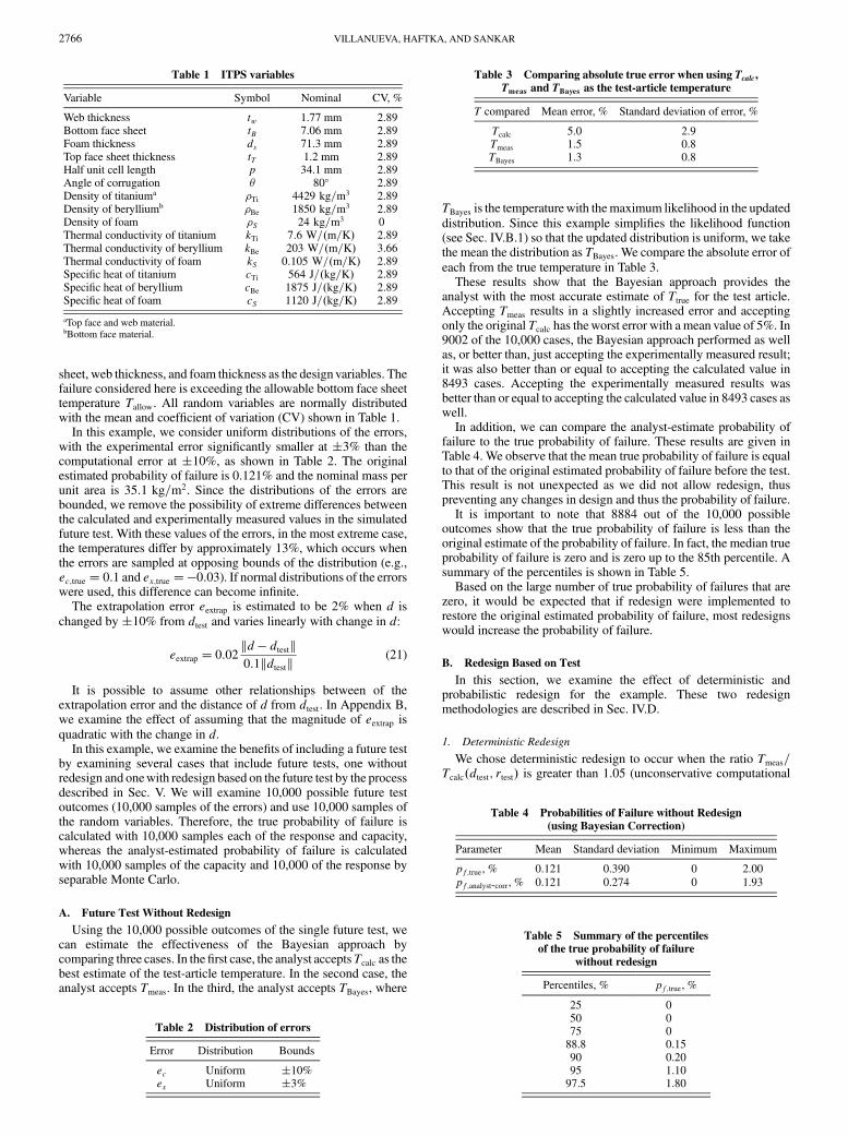
sheet, web thickness, and foam thickness as the designvariables. Thefailure considered here is exceeding the allowable bottom face sheettemperature Tallow. All random variables are normally distributedwith the mean and coefficient of variation (CV) shown in Table 1.

In this example, we consider uniform distributions of the errors,with the experimental error significantly smaller at 3% than thecomputational error at 10%, as shown in Table 2. The originalestimated probability of failure is 0.121% and the nominal mass perunit area is 35:1 kg=m2. Since the distributions of the errors arebounded, we remove the possibility of extreme differences betweenthe calculated and experimentally measured values in the simulatedfuture test. With these values of the errors, in the most extreme case,the temperatures differ by approximately 13%, which occurs whenthe errors are sampled at opposing bounds of the distribution (e.g.,ec;true � 0:1 and ex;true ��0:03). If normal distributions of the errorswere used, this difference can become infinite.

The extrapolation error eextrap is estimated to be 2% when d ischanged by10% from dtest and varies linearly with change in d:

eextrap � 0:02kd � dtestk0:1kdtestk

(21)

It is possible to assume other relationships between of theextrapolation error and the distance of d from dtest. In Appendix B,we examine the effect of assuming that the magnitude of eextrap isquadratic with the change in d.

In this example, we examine the benefits of including a future testby examining several cases that include future tests, one withoutredesign and onewith redesign based on the future test by the processdescribed in Sec. V. We will examine 10,000 possible future testoutcomes (10,000 samples of the errors) and use 10,000 samples ofthe random variables. Therefore, the true probability of failure iscalculated with 10,000 samples each of the response and capacity,whereas the analyst-estimated probability of failure is calculatedwith 10,000 samples of the capacity and 10,000 of the response byseparable Monte Carlo.

A. Future Test Without Redesign

Using the 10,000 possible outcomes of the single future test, wecan estimate the effectiveness of the Bayesian approach bycomparing three cases. In thefirst case, the analyst acceptsTcalc as thebest estimate of the test-article temperature. In the second case, theanalyst accepts Tmeas. In the third, the analyst accepts TBayes, where

TBayes is the temperaturewith themaximum likelihood in the updateddistribution. Since this example simplifies the likelihood function(see Sec. IV.B.1) so that the updated distribution is uniform, we takethe mean the distribution as TBayes. We compare the absolute error ofeach from the true temperature in Table 3.

These results show that the Bayesian approach provides theanalyst with the most accurate estimate of Ttrue for the test article.Accepting Tmeas results in a slightly increased error and acceptingonly the original Tcalc has theworst error with a mean value of 5%. In9002 of the 10,000 cases, the Bayesian approach performed as wellas, or better than, just accepting the experimentally measured result;it was also better than or equal to accepting the calculated value in8493 cases. Accepting the experimentally measured results wasbetter than or equal to accepting the calculated value in 8493 cases aswell.

In addition, we can compare the analyst-estimate probability offailure to the true probability of failure. These results are given inTable 4. We observe that the mean true probability of failure is equalto that of the original estimated probability of failure before the test.This result is not unexpected as we did not allow redesign, thuspreventing any changes in design and thus the probability of failure.

It is important to note that 8884 out of the 10,000 possibleoutcomes show that the true probability of failure is less than theoriginal estimate of the probability of failure. In fact, the median trueprobability of failure is zero and is zero up to the 85th percentile. Asummary of the percentiles is shown in Table 5.

Based on the large number of true probability of failures that arezero, it would be expected that if redesign were implemented torestore the original estimated probability of failure, most redesignswould increase the probability of failure.

B. Redesign Based on Test

In this section, we examine the effect of deterministic andprobabilistic redesign for the example. These two redesignmethodologies are described in Sec. IV.D.

1. Deterministic Redesign

We chose deterministic redesign to occur when the ratio Tmeas=Tcalc�dtest; rtest� is greater than 1.05 (unconservative computational

Table 1 ITPS variables

Variable Symbol Nominal CV, %

Web thickness tw 1.77 mm 2.89Bottom face sheet tB 7.06 mm 2.89Foam thickness ds 71.3 mm 2.89Top face sheet thickness tT 1.2 mm 2.89Half unit cell length p 34.1 mm 2.89Angle of corrugation � 80� 2.89Density of titaniuma �Ti 4429 kg=m3 2.89Density of berylliumb �Be 1850 kg=m3 2.89Density of foam �S 24 kg=m3 0Thermal conductivity of titanium kTi 7:6 W=�m=K� 2.89Thermal conductivity of beryllium kBe 203 W=�m=K� 3.66Thermal conductivity of foam kS 0:105 W=�m=K� 2.89Specific heat of titanium cTi 564 J=�kg=K� 2.89Specific heat of beryllium cBe 1875 J=�kg=K� 2.89Specific heat of foam cS 1120 J=�kg=K� 2.89

aTop face and web material.bBottom face material.

Table 2 Distribution of errors

Error Distribution Bounds

ec Uniform 10%ex Uniform 3%

Table 3 Comparing absolute true error when using Tcalc,

Tmeas and TBayes as the test-article temperature

T compared Mean error, % Standard deviation of error, %

Tcalc 5.0 2.9Tmeas 1.5 0.8TBayes 1.3 0.8

Table 4 Probabilities of Failure without Redesign

(using Bayesian Correction)

Parameter Mean Standard deviation Minimum Maximum

pf;true, % 0.121 0.390 0 2.00pf;analyst-corr, % 0.121 0.274 0 1.93

Table 5 Summary of the percentilesof the true probability of failure

without redesign

Percentiles, % pf;true, %

25 050 075 088.8 0.1590 0.2095 1.1097.5 1.80

2766 VILLANUEVA, HAFTKA, AND SANKAR

model) or less than 0.95 (conservative computational model). Weconsider one design variable, the foam thickness ds. This variablewas chosen because it has a large impact on the bottom face sheettemperature. The results including deterministic redesign are given inTable 6.

These results show that the true probability of failure is greatlyreducedwhen redesign is allowed. In addition, the standard deviationis also reduced. Since the redesign is symmetric, it does not causemuch change in the average mass. The reason for this drasticreduction in probability of failure is the substantial reduction in errorthat allowed us to redesign all the designs that had a probability offailure above 0.121%. So while the system was designed for aprobability of failure of 0.121%, it ended up with a mean probabilityof failure of 0.0007%.

However, we note a large standard deviation in ds, with theminimum andmaximum values quite different from the design valueof 71.3 mm. In practice, the redesign may not be allowed to be thisdrastic. Therefore, we also examine the case where the bounds of theredesigned ds are restricted to 10% of the original nominal dS.These results are given in Table 7.

We observe that restricting the bounds of dS does not change thetrue probability of failure and does not cause a significant change inthe average mass.

2. Probabilistic Redesign

The initial design does not necessarily meet the reliabilityrequirements of the designer. It can be, for example, a candidatedesign in a process of design optimization. When it comes to proba-bilistic redesign, one may examine redesign to the mean probabilitywithout redesign or to a target probability. Here we assume the latter,and we examine cases where the target redesign probability ispf;target � 0:01% with and without bounds on ds. Here, we requireredesign to occur when the estimated probability of failure is not

within 50% of the target. We require that all unconservative(dangerous) designs above the 50% threshold be redesign, but rejectthe redesign of overly conservative cases if itsmass does not decreaseby at least 4.5%. Since only one design variable, the foam thickness,is considered, a decrease in mass can only result from a decrease infoam thickness, which causes an increase in temperature. The resultsare shown in Table 8.

Without bounds on the redesigned ds, we observe that the analyst-estimated target probability of failure is close to the target of 0.01%. Itis also observed that there is a significant reduction in mass (4%reduction) and a reduction in the original mean true probability offailure from 0.121 to 0.003%. The analyst is able to estimate this trueprobability of failure with reasonable accuracy.

Whenwe include the bounds onds, the true probability of failure isunable to converge to the target probability of failure, but there isbetter agreement between the analyst-estimated probabilities offailure and the true value. This is due to the inclusion of theextrapolation error in the probability of failure in the redesignprocess. We also observe a 1.7% reduction in mean mass from theoriginal value.

On a final note, we recognize that the large percentage of redesignsare undesirable. This percentage can be greatly reduced by lessstringent redesign rules, while still having very low probabilities offailure.

VII. Conclusions

This study presented a methodology to include the effect of asingle future test followed by redesign on the probability of failure ofan integrated thermal protection system. Two methods of calibrationand redesign based on the test were presented. The deterministicapproach, which represents current design/redesign practices, leadsto a greatly reduced probability of failure after the test and redesign, areduction that is usually not quantified.

Table 6 Calibration by the correction factor approach with deterministic redesign

Parameter Original Mean Standard deviation Minimum Maximum

dS, mm 71.3 71.5 1.2 44.8 99.4Mass, kg=m2 35.1 35.1 2.8 28.9 41.6pf;true, % 0.121 0.0007ab 0.009 0 0.200

aOf the 10,000 possible outcomes of the future test, 4964 required redesign. Conservative cases account for 2425 ofthe redesigns, and unconservative cases account for 2539.bFor the true probability, 99.3% are below the mean.

Table 7 Calibration by correction factor with deterministic redesign, bounds of redesignedds restricted to �10% of original ds

Parameter Original Mean Standard Deviation Minimum Maximum

dS, mm 71.3 71.4 0.5 64.1 78.4mass, kg=m2 35.1 35.1 1.2 33.4 36.7pf;true, % 0.121 0.0007 0.009 0 0.200

Table 8 Calibration by the Bayesian-updating approach with probability of failure based redesign (pf ;target � 0:01%)

Restriction on redesigned ds Parameter Original Mean Standard deviation Minimum Maximum

No bounds dS, mm 71.3 65.3 8.9 47.5 77.7mass, kg=m2 35.1 33.7 2.1 29.5 36.5pf;true, % 0.121 0.003ab 0.016 0 0.100

pf;analyst-corr, % 0.121 0.007 0.004 0 0.015Within 10% of dtest dS, mm 71.3 68.8 5.1 64.1 77.7

mass, kg=m2 35.1 34.5 1.2 33.4 36.5pf;true, % 0.121 0.003 0.016 0 0.100

pf;analyst-corr, % 0.121 0.003 0.005 0 0.015

aOf the 10,000 possible outcomes of the future test, 7835 are redesigned. With the requirement of a 4.5% decrease in mass, 5126 of the 7001conservative models (pf;analyst < pf;target) are redesigned. For unconservative designs, 2709 are redesigned.bFor the true probability, 97.4% are below the mean.

VILLANUEVA, HAFTKA, AND SANKAR 2767

The probabilistic approach includes the Bayesian technique forcalibrating the temperature calculation and redesign to a targetprobability of failure. It provides a way to more accurately estimatethe true probability of failure after the test. In addition, it allowsweight to be traded against performing additional tests.

Though the methodology is presented in the context of a futurethermal test and redesign on the ITPS, the methodology is applicablefor estimating the reliability of almost any component that willundergo a test followed by possible redesign. Given a computationalmodel, uncertainties, errors, and redesign procedures, along with thestatistical distributions, the procedure of simulating the future testresult by Monte Carlo sampling, calibration, and redesign can bereadily applied.

Futurework includes incorporating the effect of the future test intothe optimization of the ITPS. This study has brought to light manytunable parameters in the test, such as the bounds on the designvariables, the target probability of failure for redesign, and theredesign criterion itself. Including these parameters into the opti-mization will not only optimize the design, but will optimize the testas well.

Appendix A: Comparison of Bayesian Formulations

In a rigorous formulation of the likelihood function, we wouldcalculate the conditional probability of obtaining the measuredtemperature when the true temperature of the test article is T, asshown in Eq. (A1):

ltest�T� �(

10:14T

if

����T�Tmeas

T

����� 0:07;

0 otherwise

(A1)

In the illustrative example in Sec. IV.B.1, we simplified thisformulation so that we calculated the conditional probability ofobtainingT givenTmeas, as shown inEq. (17). In Fig.A1,we comparethe two likelihood functions and the resulting updated distribution of

fupdtest;Ptrue for the case in the example.

The figures show only a small difference in the bounds of theupdated temperature distribution and the values of the PDFs. Acomparison is shown in Table A1.

Appendix B: Extrapolation Error

In this paper, we assumed the variation in the magnitude of theextrapolation error eextrap was linear with the distance of the designfrom the test design. The choice of this extrapolation error is verymuch up to the analyst, as it is a measure in the variation of the errorsfrom the updated Bayesian estimate away from the test design. Here,we examine the effect of an assumption that the extrapolation error isquadratic, as expressed in Eq. (B1):

eextrap � �eextrap�max

�kd � dtestk�dlim

�2

(B1)

For the example problem in Sec. VI, we estimated eextrap to be 2%when d is changed by 10% from dtest. With the quadraticextrapolation error, this is expressed as in Eq. (B2). Because of thisrequirement, the magnitude of the quadratic extrapolation error issmaller for designs at a distance less than10% away from the testdesign, but larger at greater distances, compared with the linearvariation. We present this comparison in Fig. B1. Examining thesame 10,000 possible outcomes of the future test with probabilisticredesign (pf;target � 0:01%), the results in Table B1 were obtained:

eextrap � 0:02

�kd � dtestk0:1kdtestk

�2

(B2)

The results show that there is improved agreement between thetrue and analyst-estimated probabilities of failure, as well as aslightly decreased mass and variation in the mass, with the quadraticvariation in extrapolation error. Since the extrapolation error issmaller at a distance less than10% away from the test design, theagreement between the true and analyst-estimated probabilities offailure is better with the quadratic extrapolation error. However, theagreement still suffers, due to the large magnitude of theextrapolation error at distances greater than 10%.

Fig. A1 Illustrative example of Bayesian updating using the likelihood about Tmeas (top) and the likelihood about T (bottom).

Table A1 Comparison of fupdtest;Ptrue with different formulations of the likelihood function

Comparison ltest�T� about Tmeas ltest�T� about TBounds where updated distribution is nonzero [0.9765, 1.1] [0.9813, 1.1]

Max fupdtest;Ptrue and location 8.1 on [0.9765, 1.1] 8.9 at T � 0:9813

2768 VILLANUEVA, HAFTKA, AND SANKAR

Acknowledgments

This material is based upon work supported by NASA underaward no. NNX08AB40A. Any opinions, findings, and conclusionsor recommendations expressed in thismaterial are those of the author(s) and do not necessarily reflect the views of the NationalAeronautics and Space Administration.

References

[1] Fujimoto, Y., Kim, S. C., Hamada, K., and Huang, F., “InspectionPlanning Using Genetic Algorithm for Fatigue DeterioratingStructures,” Proceedings of the International Offshore and Polar

Engineering Conference, Vol. 4, International Society of Offshore andPolar Engineers, Golden, CO, 1998, pp. 99–109.

[2] Toyoda-Makino,M., “Cost-BasedOptimalHistoryDependent Strategyfor Random Fatigue Cracks Growth,” Probabilistic Engineering

Mechanics, Vol. 14, No. 4, Oct. 1999, pp. 339–347.doi:10.1016/S0266-8920(98)00042-3

[3] Garbatov, Y., and Soares, C., “Cost and Reliability Based Strategies forFatigue Maintenance Planning of Floating Structures,” Reliability

Engineering and System Safety, Vol. 73, No. 3, 2001, pp. 293–201.doi:10.1016/S0951-8320(01)00059-X

[4] Kale, A., and Haftka, R. T., “Tradeoff of Weight and Inspection Cost inReliability-Based Structural Optimization,” Journal of Aircraft,Vol. 45, No. 1, 2008, pp. 77–85.doi:10.2514/1.21229

[5] Kale, A., Haftka, R. T., and Sankar, B. V., “Efficient Reliability-BasedDesign and Inspection of Panels Against Fatigue,” Journal of Aircraft,Vol. 45, No. 1, 2008, pp. 86–96.doi:10.2514/1.22057

[6] Acar, E., Haftka, R. T., and Kim, N. H., “Effects of Structural Tests on

Aircraft Safety,” AIAA Journal, Vol. 48, No. 10, 2010, pp. 2235–2248.doi:10.2514/1.J050202

[7] Acar, E., Haftka, R. T., Kim, N. H., and Buchi, D., “Including theEffects of Future Tests in Aircraft Structural Design,” 8th World

Congress for Structural and Multidisciplinary Optimization, Lisbon,Portugal, June 2009.

[8] Villanueva, D., Sharma, A., Haftka, R. T., and Sankar, B. V., “RiskAllocation by Optimization of an Integrated Thermal ProtectionSystem,” 8th World Congress for Structural and Multidisciplinary

Optimization, Lisbon, Portugal, June 2009.[9] Bapanapalli, S.K., “Design of an Integrated Thermal Protection System

for Future Space Vehicles,” Ph.D. Dissertation, University of Florida,Gainesville, FL, 2007.

[10] Gogu, C., Haftka, R. T., Bapanapalli, S. K., and Sankar, B. V.,“Dimensionality Reduction Approach for Response SurfaceApproximations: Application to Thermal Design,” AIAA Journal,Vol. 47, No. 7, 2009, pp. 1700–1708.doi:10.2514/1.41414

[11] Oberkampf,W.L., Deland, S.M., Rutherford, B.M., Diegert, K.V., andAlvin, K. F., “Error and Uncertainty in Modeling and Simulation,”Reliability Engineering and System Safety, Vol. 75, No. 3, 2002,pp. 333–357.doi:10.1016/S0951-8320(01)00120-X

[12] Smarslok, B. P., Haftka, R. T., Carraro, L., and Ginsbourger, D.,“Improving Accuracy of Failure Probability Estimates with SeparableMonte Carlo,” International Journal of Reliability and Safety, Vol. 4,2010, pp. 393–414.doi:10.1504/IJRS.2010.035577

R. KapaniaAssociate Editor

Fig. B1 Comparison of the eextrap with linear and quadratic variation with the distance of the design from the test design (test design is d� 71:3 mm).

Table B1 Calibration by the Bayesian-updating approach with probability of failure based

redesign (pf ;target � 0:01%), quadratic extrapolation error, and no bounds on redesign dS

Parameter Original Mean Standard Deviation Minimum Maximum

Linear variation in eextrap with dsdS, mm 71.3 65.3 8.9 47.5 77.7Mass, kg=m2 35.1 33.7 2.1 29.5 36.5pf;true, % 0.121 0.003 0.016 0 0.100pf;analyst-corr, % 0.121 0.007 0.004 0 0.015

Quadratic variation in eextrap with dsdS, mm 71.3 66.4 7.3 54.4 77.1Mass, kg=m2 35.1 33.9 1.7 31.1 36.4pf;true, % 0.121 0.004 0.019 0 0.100pf;analyst-corr, % 0.121 0.007 0.004 0 0.015

VILLANUEVA, HAFTKA, AND SANKAR 2769