Including biogeochemical factors and a temporal component in benthic habitat maps: influences on infaunal diversity in a temperate embayment

Including biogeochemical factors and a temporalcomponent in benthic habitat maps: influenceson infaunal diversity in a temperate embayment

Lynda C. RadkeA,C, Zhi HuangA, Rachel PrzeslawskiA, Ian T. WebsterB,Matthew A. McArthurA, Tara J. AndersonA, P. Justy SiwabessyA

and Brendan P. BrookeA

AMarine and Coastal Environment Group, Geoscience Australia, GPO Box 378,

Canberra, ACT 2601, Australia.BCSIRO Land and Water, Canberra, ACT 2601, Australia.CCorresponding author. Email: [email protected]

Abstract. Mapping of benthic habitats seldom considers biogeochemical variables or changes across time.We aimed to:(i) develop winter and summer benthic habitat maps for a sandy embayment; and (ii) compare the effectiveness of various

maps for differentiating infauna. Patch types (internally homogeneous areas of seafloor) were constructed usingcombinations of abiotic parameters and are presented in sediment-based, biogeochemistry-based and combinedsediment–biogeochemistry-based habitat maps. August and February surveys were undertaken in Jervis Bay, NSW,

Australia, to collect samples for physical (% mud, sorting, % carbonate), biogeochemical (chlorophyll a, sulfur, sedimentmetabolism, bioavailable elements) and infaunal analyses. Boosted decision tree and cokrigingmodels generated spatiallycontinuous data layers. Habitat maps were made from classified layers using geographic information system (GIS)overlays and were interpreted from a biophysical-process perspective. Biogeochemistry and % mud varied spatially and

temporally, even in visually homogeneous sediments. Species turnover across patch types was important for diversity; theutility of habitat maps for differentiating biological communities varied across months. Diversity patterns were broadlyrelated to reactive carbon and redox, which varied temporally. Inclusion of biogeochemical factors and time in habitat

maps provides a better framework for differentiating species and interpreting biodiversity patterns than once-off studiesbased solely on sedimentology or video-analysis.

Additional keywords: benthic habitat mapping, beta-diversity, macroalgal detritus, marine environmental management,polychaete mounds, surrogacy.

Received 13 May 2011, accepted 3 September 2011, published online 25 October 2011

Introduction

Marine benthic maps comprise sets of patches (i.e. internallyhomogeneous areas of seafloor) that are repeated in space (Zajac

2008a). Such patches are often equatedwith habitats andmay bevaluable surrogates for biodiversity because they representenvironmental variations that can influence the distribution and

abundance of organisms (Anderson et al. 2009a). The recentfocus on biodiversity surrogates is due to the high costs asso-ciated with direct biological sampling and analysis (particularly

in deep and remote areas). It is generally more cost-effective tomap or physically sample seabed environments than to under-take biological sampling and taxonomic identifications oversimilar spatial extents. Indeed, limited biological data has

caused a shift in recent decades from a conservation of speciesapproach to marine environmental management to a conserva-tion of spaces approach (Zacharias and Roff 2000; Huang et al.

2011). For example, abiotic datasets have been used to

inform the Australian marine bioregionalisation (Department ofEnvironment and Heritage 2005) and marine protected areas(MPAs) (Harris et al. 2008).

Acoustic and underwater video technologies are widelyadopted approaches for seabed mapping and identifying poten-tial habitats (Huang et al. 2009; NSW Marine Parks Authority

2010). For example, high resolution multibeam systems areparticularly well suited to delineating sandy from rocky habitats(Todd and Greene 2007). However, multibeam acoustic tech-

nologies are often less effective for mapping soft-sedimentenvironments because of generally smaller variations in acous-tic reflectivity. This is an important consideration given thatsandy sediments are found over,70% of the global continental

shelf (Emery 1968). Seabed maps for management have alsobeen developed by interpolating and combining environmentaldatasets to form mosaics of different patch types (Harris and

Whiteway 2009; Huang et al. 2011). The utility of suchmaps for

CSIRO PUBLISHING

Marine and Freshwater Research, 2011, 62, 1432–1448

http://dx.doi.org/10.1071/MF11110

Journal compilation � CSIRO 2011 www.publish.csiro.au/journals/mfr

species conservation/surrogacy has recently been tested usingbiological data, demonstrating that they are biologically valid in

some circumstances (Przeslawski et al. 2011).Most sandy seabed environments have been mapped on the

basis of geomorphological (topographic) and sediment charac-

teristics (i.e. grain size and sorting) wherein benthic seascapeelements comprise low relief topographic features such as sandwaves (Thrush et al. 2005; Zajac 2008b). However, the distri-

bution patterns of benthic organisms reflect historical andevolutionary factors and interactions between a large suite ofbiophysical factors (salinity, temperature, oxygen concentra-tions, current energy, bathymetry, surface productivity,

substrate composition and sedimentation; Snelgrove 1999)and there are many potential abiotic surrogates of biodiversity(McArthur et al. 2010). The relative importance of these

variables depends on scale and on the situation of the studyarea as it relates to environmental gradients (Thrush et al.

2005). Biogeochemical properties of the seabed are not gener-

ally incorporated into benthic habitat maps, despite the wellknown role of biogeochemical processes in regulatingthe availability of carbon and nutrients at the seafloor andwithin the seabed.

Ocean surface productivity has been used as a benthic foodabundance layer in a global seascapemap (Harris andWhiteway2009). This was appropriate for the scale because the ocean-

wide pattern of sediment total organic carbon (TOC) concentra-tions (and burial rates) roughly corresponds with surface waterprimary productivity (Seiter et al. 2004). However, this simple

relationship is decoupled at smaller spatial scales because ofvariability in sedimentary and biogeochemical processes (Seiteret al. 2004). Moreover, refractory organic compounds, derived

principally from soils, physically associate with fine-grainedminerals where they are protected from chemical oxidation(Wagai andMayer 2007; Zonneveld et al. 2010). Consequently,TOC concentrations in fine sediments, which are widely

measured (Seiter et al. 2004), often reflect the surface areaand dynamics of sediment grains (Emerson and Hedges 2003)but not necessarily the amount of carbon available to consumers.

Food availability is a major source of spatial and temporalvariability in soft sediments (Kelaher and Levington 2003;Ramey and Bodnar 2008). Biogeochemical reactions further

contribute to sediment patchiness and, when conducive toanoxia, can substantially reduce the diversity and abundanceof benthic invertebrates (Kelaher and Levington 2003). Tempo-ral mosaics of disturbances and spatial heterogeneity help to

maintain marine diversity (reviewed by Zajac 2008a) but at thescale of benthic seascapes, there is almost a complete lack ofdata to allow assessments to be made of how seabed patches

change over time (Zajac 2008b). In sandy sediments, organicmatter (OM) decomposition pathways can be highly variable(aerobic to sulfate reduction) depending on the availability of

labile OM,water temperature and on factors that influence pore-water exchange rates (i.e. degree of permeability, biologicalactivity, wave-action and interactions between topography and

bottom current) (Cook et al. 2007). These factors may vary ontimescales ranging from minutes to months, creating spatiallycomplex and highly dynamic biogeochemical settings noted forpatchiness in oxygen, nutrients, metals and sulfides, as well as

OM (Janssen et al. 2005; Franke et al. 2006; Cook et al. 2007).

The utility of habitat maps in differentiating biological commu-nities may therefore vary across months, seasons, or years, but

this variation is rarely addressed in surrogacy ormapping studies(McArthur et al. 2010).

The fundamental objective of this studywas todevelopbenthic

habitat maps for a sandy temperate embayment. Patch types weredelineated by various combinations of abiotic parameters and arepresented in the format of sediment-based, biogeochemistry-

based and combined sediment–biogeochemistry habitat maps.Both winter and summer datasets were mapped to capture therange in the biogeochemical attributes of sediments that areexpected in response to seasonal differences in water temperature

and primary productivity. However, because of a lack of replica-tion in seasonal data, our results cannot be interpreted as due toseason per se. Our second objective was to compare maps of

varying complexity (i.e. video-based, sediment-based and com-bined sediment–biogeochemistry-based) in terms of their relativeeffectiveness (‘validity’) for differentiating infaunal assemblages

(Crustacea), because benthic habitat maps are often used toinfer biodiversity patterns in the absence of biological data(i.e. as biodiversity surrogates). Strong emphasis was placed onthe interpretation of maps and biological associations in relation

to the broad pattern of biophysical processes within the studyarea. A companion study, based on the same data acquisitionprogram (winter only), will develop robust techniques to explic-

itly test surrogacy relationships between individual physical–biogeochemical variables and co-located infauna (Z. Huang,M. McArthur, L. Radke, T. Anderson, S. Nichol, J. Siwabessy

and B. Brooke, unpubl.data). The current study provides theessential spatial context for those variables.

Study area and data

Study area

This study examines a 3� 5 km area of complex soft sediment

seabed adjacent to the entrance of Jervis Bay called the DarlingRoadGrid (DRG) (Fig. 1; Anderson et al. 2009b). Jervis Bay is alarge (115 km2) semi-enclosed embayment on the south coast of

NSW (358070S, 1508420E; Fig. 1a) and has been classified as‘largely unmodified’ (Heap et al. 2001). The Bay is exposed tohighly variable offshore sea and swell emanating primarily from

the south-east and shallow-water refraction, diffraction andfrictional attenuation causes a reduction in the wave-energywithin the Bay. Jervis Bay is flushed approximately weekly andtidal currents are weak (,0.01m s�1) apart from at the entrance

(0.07m s�1) (Holloway et al. 1992).Much of the seabed within Jervis Bay comprises fine–

medium quartz sand with minor carbonate (Taylor 1972).

Average seabed TOC concentrations (�s.d.) across the gridwere 0.2� 0.2% at the time of the survey. A variety of complexand biologically important benthic habitats have been recorded

within the Bay (i.e. drift algae (commonly dominated byGracilaria edulis and Acrosorium venulosum), polychaetehummocks (chaetopterid worm Mesochaetopterus minutus),

rippled and bioturbated sands, bivalve clumps and hearturchin (Echinocardium cordatum) areas) in an earlier study(CSIRO 1993).

At the times of our surveys, bottom water temperatures

(�s.d.) were 14.1� 0.58C (27–29 August 2008) and

Benthic habitat mapping of sandy soft sediments Marine and Freshwater Research 1433

16.3� 0.28C (9–12 Feb 2009). Surface water temperatures werenot statistically different from bottom waters during the wintersurvey, but were 3–48C higher in the summer months. Bottom

waters were generally well oxygenated, although saturationstates were lower in February (i.e. 95.5� 7%) than in August(.100%). Water depths ranged from 1 to 36m across the DRG(Fig. 1c) and all stations were within the euphotic zone for water

column productivity as defined as the water depth at whichirradiance falls to 1% of surface values (Kirk 1994).

Choice of abiotic variables

This study forms part of the ‘Surrogates Program’ in the(Australian) Commonwealth Environmental Research Facilities

Marine Biodiversity Hub. Our choice of environmental vari-ables was thus guided by a wider objective to find surrogates(maps/abiotic variables) that could be applied broadly and

relatively inexpensively. Procedures that require specialisedinstrumentation or a high level of discipline expertise were notconsidered desirable. Sorting, % mud and % carbonate were thevariables chosen to develop the sediment-based habitat maps.

These factors were considered useful surrogates of biodiversitybecause they are linked to food availability, size of sedimentinterstices and substrate composition (reviewed by McArthur

et al. 2010). For the biogeochemistry-based maps, we used

variables that provide information on the nutritional quality ofsediment and redox status (Radke et al. 2011). We measuredchlorophyll a (Chl a) to quantify the highly labile component of

the OM pool that was due to fresh phytoplankton/microphyto-benthos. In addition, we applied a total sediment metabolism(TSM) measure to estimate the bulk OM reactivity/quality ofour sediment samples. TSM should not be confused with actual

(in situ) rates of OM decay, which would be strongly influencedby enhanced pore-water exchange in these sandy sediments(Cook et al. 2007). Bioavailable bioactive trace elements (BAE)

(i.e. acid-extractable Mn, Fe, Co, Ni, Cu and Zn) were alsomeasured on the supposition that these could be potentiallylimiting resources in sandy sediments of relatively unmodified

settings (see, for example, Sterner and Hessen 1994). Finally,total sulfur (TS) concentrations were used because they mayrecord the process of bacterial sulfate reduction in sediment

(Berner 1984). Hydrogen sulfide gas is produced during thisanoxic process and reacts with iron to form the sulfide-bearingminerals pyrite (FeS2) and iron mono-sulfides (FeS). It was ourinitial intention to use S : Fe ratios rather than TS in the maps.

However, unusually high Fe concentrations (likely due togroundwater discharge) were identified in about one-third of theAugust samples in a preliminary assessment (Fe vs. S) and TS

was deemed more appropriate for our purposes. However, in

34�50�0�S

35�0�0�S

Currambene Creek

CararmaCreek

Jervis Bay

Legend

Study area

Land

N

0 3.75 7.5 15km

1

36

Samples – Feb 09�

Samples – Aug 08�

Depth (m)Moona Moona Creek

PointPerpendicular

BowenIsland

GovernorHead

35�10�0�S

35�5�0�S

35�5�30�S

35�6�0�S

35�6�30�S

35�7�0�S

35�7�30�S

35�8�0�S

35�8�30�S

35�5�0�S

35�6�0�S

35�7�0�S

35�8�0�S

150�40�0�E 150�50�0�E 150�43�0�E 150�44�0�E 150�45�0�E 150�46�0�E

150�42�30�E 150�43�30�E 150�44�30�E 150�45�30�E 150�46�30�E

(a) (b)

(c)

Fig. 1. (a) Location of study area (Darling Road Grid) within Jervis Bay, NSW, Australia. (b, c) Sample locations for August and February respectively.

The bathymetry is shown in (c).

1434 Marine and Freshwater Research L. C. Radke et al.

some cases we drew upon Fe : S ratios to further develop redoxarguments.

Methods

Field methods

Co-located benthic samples for infauna plus sedimentology andbiogeochemistry (accuracy of #8m) were collected from

throughout the DRG at pre-determined stations (Fig. 1b, c)during 27–29 August 2008 (austral winter; 32 stations andsamples) and 9–12 February 2009 (austral summer; 32 stations

with 51 samples). We used a Shipek-style grab (GeoscienceAustralia, Canberra, ACT) to collect sediment samples forgeochemical analysis and a small VanVeen grab for the infauna/

sedimentology analysis (Anderson et al. 2009b; Przeslawskiet al. 2009a). Sediments collected in the Van Veen grab(Geoscience Australia) were sieved through a 500 mm sieve

(further details given by Anderson et al. 2009b; Przeslawskiet al. 2009a). Sievedmaterial was then preserved in 99%ethanolfor sorting back in the laboratory.

The Shipek sampler collected intact samples of sediment

(and porewater) up to 5� 12 cm in area and 5 cm thick. Imme-diately after grab recovery, the surface sediments weresubsampled into five separate containers for the following

analyses: (i) porosity and bulk density (0–2 cm); (ii) potentiallybioavailable trace elements (0–2 cm; 10mL volumetric bottleswhich were acid-washed before use); (iii) Chl a concentrations

(0–0.5 cm; 10mL volumetric bottles wrapped in aluminiumfoil); and (iv–v) vial incubations (TCO2 production/TSM) andsolid-phase chemistry (,0–2 cm; two 58mL Falcon vialscompletely filled with sediment).

The porosity andChl a samples were frozen immediately andthe Falcon vials were wrapped in aluminium foil and placed ina container in which seawater was held at in situ bottom water

temperatures. No later than 4 h after collection, the porewatersfrom one of the two Falcon vials (time¼ zero (t0)) wereextracted by centrifugation (93.2Hz; 5min) and syringe-filtered

(0.45 mm) into 3mL exetainers that had been pre-charged with0.025mL of mercuric chloride (to poison the samples). Approx-imately 24 h later, the second of the two Falcon vials from each

site (time¼ one (t1)) was sampled by the same method. Theporewater extracts were stored in the refrigerator before analysisfor TCO2 concentrations, while the residual bulk sediments(t0 samples only) were frozen for subsequent solid-phase

determinations.

Analytical techniques

TCO2 was analysed using an AS-C3 DIC analyser (Apollo

SciTech, Bogart, GA, USA), which includes a Li-Cor 7000infrared-based CO2 detector (Li-Cor Biosciences, Lincoln,NE, USA). A certified reference material for CO2 measure-

ments was used as a standard (Scripps Institute of Oceanog-raphy, San Diego, CA, USA). The average precision (�s.d.) ofthe batches was 0.2� 0.1mmol kg�1. Accuracy was assessed

with the analysis of 0.002M Na2CO3 solutions with each ofthe batches and the results were always within 1.0� 0.4%of expected values. Mineralisation rates were estimatedas mmol CO2 produced cm�3 day�1 by using the porosity/bulk

density data.

Major and trace elements (including %SO3 and Fe2O3) weredetermined on the solid-phase by X-ray fluorescence (XRF) at

Geoscience Australia using a Phillips PW204 4kW sequentialspectrometer (PANalaytical BV, Almelo, The Netherlands)calibrated with SARM and USGS rock standards. The TS

concentrations were corrected for seawater salts using the Clconcentrations. Hydrochloric acid (HCl) metal digests of sedi-ments were also undertaken following the protocol of Snape

et al. (2004). Briefly, 20mL of a 1M HCl solution and 1 gfreeze-dried sediment were mixed for 4 h at room temperature,before centrifugation and then filtered into acid-cleaned con-tainers. The HCl extracts were analysed by quadrupole ICP-MS

(Perkin Elmer DLC 111, Waltham, MA, USA) at the Universityof Canberra. All major interfering elements/compounds (i.e. ClonV, Cr, As and Se)were checked and corrected for. A principal

component analysis on the acid-extractable (bioavailable) frac-tion found that, with the exception of Cd, all of the bioactiveelements had the highest scores on the first principal component.

We used the axis 1 site scores of this analysis as an indicator ofBAE availability in our subsequent analyses to reduce thenumber of variables in the classification.

Proportions of mud, sand and gravel were determined using

standard mesh-sieves and a Malvern Mastersiser 2000 (ATAScientific, Sydney, NSW) laser particle size analyser was usedto obtain volumetric grainsize curves for the ,2mm fraction.

The sediment sorting parameter was derived from the lasergrainsise output using the computer program GRADISTAT(Blott and Pye 2001). Carbonate contents were determined by

the carbonate bomb method by Muller and Gastner (1971).Sediment surface areas were determined using a five-pointBrunauer-Emmett-Teller (BET) adsorption isotherm on aQuan-

tachrome NOVA 2200e analyser (Quantachrome Instruments,Brisbane, Qld), with nitrogen used as the absorbate. The sampleswere first cleaned of OM by slow heating over 12 h to 3508C,followed by an overnight cooling period. Chl a concentrations in

sediment extracts (90% acetone) were calculated from spectro-photometric readings at wavelengths of 664 nm and 750 nmbefore and after the addition of 0.1mol L�1 HCl using the

equation derived by Lorenzen (1967).

Construction and analysis of habitat maps

The steps undertaken to construct and analyse benthic habitatmaps can be summarised as follows: (i) continuous layers were

created from the abiotic survey data; (ii) classified mapswere made from the continuous layers; (iii) habitat maps wereconstructed from the classified maps using GIS overlay

approach; and habitat maps were analysed to determine (iv)levels of abiotic heterogeneity; and (v) relationships withbiological diversity measures.

Step 1: Construct continuous layers from survey data

Boosted decision tree (BDT) (Friedman 1999a, 1999b)and cokriging were each applied to the biogeochemistry and

sediment variables. BDT is a machine-learning model that hasrobust prediction performance, especially in dealing withnon-linear relationships between explanatory and targetvariables (i.e. Leathwick et al. 2006; Pittman et al. 2009).

Cokriging uses both autocorrelation of the variable of interest


and cross-correlations between the primary variable and theancillary variables. Theoretically, cokriging should perform as

well as (if there is no cross-correlation) or better than ordinarykriging (if there is cross-correlation). Indeed, many studies havedemonstrated its superior performance over ordinary kriging

(i.e. Ersahin 2003; Leecaster 2003; Wu et al. 2009).We used the geostatistical extension ofArcGISDesktop (ver.

9.3, ESRI, Redlands, CA, USA) for cokriging, with water depth

as the only ancillary variable. This is because water depth oftenintegrates the effects of several other processes that may influ-ence the distributions of the sediment and biogeochemicalvariables used in this study (Gogina et al. 2010). The statistics

at the sample locations show that the water depth has moderatecorrelations with the three sediment variables and one biogeo-chemical variable and notable correlations with another two

biogeochemical variables (see Section A of the AccessoryPublication to this paper). The combinations of three semi-variogram model types and four neighbourhood sector types

were explored when implementing the cokriging method. Allother parameters were set at default. The combination with thehighest percentage of variance explained (R2) (from leave-one-out cross-validation) was used to generate the continuous

layer of each target variable.For the BDT, high quality multi-beam sonar bathymetry and

backscatter datasets collected in December 2007 and May 2008

(Anderson et al. 2009b), provided full coverage of the DRG andwere gridded at 1m resolution. Seven variables were derivedfrom the multibeam data (slope, aspect, topographic relief,

topographic position index, surface area, local Moran’s I forbathymetry and local Moran’s I for backscatter) and these werecalculated at four spatial scales: 3, 7, 11 and 19m (Huang et al.

2009; Verfaillie et al. 2009). Therefore, with bathymetry andbackscatter, we had a total of 30 variables (as nine variablegroups) for the modelling of the biogeochemistry and sedimentvariables using BDT. There were moderate correlations

between the variable groups of slope, topographic relief andsurface area. However, these correlations would not adverselyaffect the BDT model because of its inherent advantage in

dealing with high-dimensional (often correlated) input data(e.g. De’ath and Fabricius 2000). We used DTREG software(http://www.dtreg.com/, accessed 1 September 2011) for the

implementation of BDT. This study experimented with different

combinations of model parameters (e.g. maximum number oftrees, depth of individual trees, minimum size node to split and

number of cross-validation folds) and explanatory variablegroups to find the best performing BDT model for each targetvariable. The best performing BDT was taken to be the one that

explained the highest percentage of variance (R2) for the cross-validation evaluation (see Section B of the Accessory Publica-tion to this paper, for the details of the modelling process). This

optimal BDT was used to generate the continuous layers foreach of the target variables.

Layers with better prediction performance, measured interms of statistical accuracy (R2 values) and visual assessment,

were selected for use in habitat maps from the two sets ofresultant layers (i.e. BDT and cokriging). There is not a univer-sal guideline on the acceptable R2 value. An R2 value of ,0.3

was deemed an acceptable statistical performance for this study.

Step 2: Make classified maps from continuous layers

The individual biogeochemistry and sedimentology vari-ables were classified into two or three categories (Table 1).

Biogeochemistry variables were divided into three classes basedon approximately equal intervals because there was no existingclassification system or appropriate datasets from which to

derive a more ecologically robust schema. Established classifi-cation systems were used for the sedimentology variables.

Steps 3 and 4: Create habitat maps and analyse thesemaps for heterogeneity

Separate habitat maps were generated for sedimentology andbiogeochemistry (August and February) by combining the rele-

vant classificationmaps, cell by cell. Each unique combination ofclasses was assigned a new patch type. Combined habitat mapsfor August and February were then created by amalgamating thebiogeochemistry and sedimentology outputs by the procedures

just described. Only patch types with areas of 10 000 cells(0.25 km2) or greater are shown in the maps due to the inherentdifficulty in distinguishing so many patch types using carto-

graphic means. In addition, the 15, 20 and 25m isobaths andthe habitats identified in towed video by CSIRO (1993) wereoverlaid onto the classified maps and habitat maps to provide

focal points for our discussion. The spatial pattern of physical

Table 1. Class boundaries of the geochemistry and sediment variables

PCA, principal components analysis; N/A, not applicable

Variable Class 1 Class 2 Class 3

Total sulfur (mg m�2) Low (,0.8) Moderate (0.8, 1.3) High (.1.3)

Chlorophyll a (mg DW) Low (,0.9) Moderate (0.9, 1.8) High (.1.8)

Total sediment metabolism (mmol cm�3 day�1) Low (,1.1) Moderate (1.1, 2.2) High (.2.2)

Bioactive elements PCA scores High (,1.7) Moderate (�1.7, 1.7) Low (.1.7)

SortingA N/A Moderately sorted (1.41, 2) Poorly sorted (2, 4)

CaCO3 (%)B Silica (0, 10) Calcareous silica (10, 50) N/A

Mud (%)C Sand (0, 10) Muddy sand (10, 50) N/A

ABlott and Pye (2001).BPoulos (1988).CFolk (1980).


http://www.dtreg.com/

heterogeneity was assessed with focal variety analysis (FVA)(Harris and Whiteway 2009; Huang et al. 2011) using a circular

windowof 10 cells in radius (i.e. 10m radius) inArcGISDesktop.

Step 5: Determine relationships between habitatclassifications and diversity measures

In the laboratory, August animals were sorted and identifiedto species or recognisable taxonomic units using publishedtaxonomy and field guides (Stoddard and Lowry 2003; Cohen

et al. 2007) and museum specialists. Due to limitations in time,only two crustacean groupswere identified tomorpho-species insummer samples. Ostracods and cumaceans were chosen torepresent infaunal biodiversity in both August and February

because they are found in a range of soft-sediment environ-ments, cover diverse trophic guilds (detritivores, carnivores,herbivores, suspension feeders), are relatively easy to process

and were correlated with the total number of infauna (seeSection C of the Accessory Publication to this paper) suggestingthat the joint diversity of these taxa is related to broader diversity

patterns within the Bay. Infaunal diversity as defined in thisstudy includes only animals .500 mm. The Shannon–Wienerdiversity index, species richness and Pielou’s evenness were

calculated from the ostracod and cumacean counts at eachstation using the statistical software package PRIMER ver.6(Clarke and Warwick 2001).

Pair-wise analyses of similarities (ANOSIMs; Clarke and

Warwick 2001) to determine whether species compositiondifferences among patch types were statistically significantwould require at least two biological samples per patch type

and this minimum requirement was seldom met in our dataset(see Section D of the Accessory Publication to this paper). As analternative multivariate analysis, we developed a VISUAL

BASIC program to calculate average Bray–Curtis dissimilarityindices between stations belonging to each patch type andstations belonging to the remaining pool of patches combined(including patch types with ,10 000 cells). When measured at

two stations (i and j), Bray –Curtis dissimilarities are defined as:

BCij ¼XS

k¼1

jðNik � NjkÞjNik þ Njk

; ð1Þ

where S is the number of species considered and Nik is thenumber of species of type k measured at site i (Clarke and

Warwick 2001). Suppose stations are ordered in such a way thatconsecutive stations belong to the same patch types. Further,

suppose there are three patch types (A, B and C) which containm, n and p stations respectively.

stn 1:::::stn mzfflfflfflfflfflfflfflfflffl}|fflfflfflfflfflfflfflfflffl{A

stnmþ 1:::::stn mþ nzfflfflfflfflfflfflfflfflfflfflfflfflfflfflfflfflfflffl}|fflfflfflfflfflfflfflfflfflfflfflfflfflfflfflfflfflffl{B

stnmþ nþ 1:::::stnmþ nþ pzfflfflfflfflfflfflfflfflfflfflfflfflfflfflfflfflfflfflfflfflfflfflfflfflfflffl}|fflfflfflfflfflfflfflfflfflfflfflfflfflfflfflfflfflfflfflfflfflfflfflfflfflffl{C

;

ð2Þ

Using patch type A as an example, the average dissimilaritybetween its elements and all the other stations was calculated as:

BCA ¼

Pm

i¼1

Pmþnþp

j¼mþ1

BCij

mðnþ pÞ ; ð3Þ

The calculated values ofBCA,BCB andBCCwere then comparedwith the values that would be computed if there were no pre-

dictive value of each grouping for the dissimilarity indices.Again using patch type A as an example, one calculates thevalues of BCA assuming that the m stations in the group are a

series of selections of all the stations available. By cyclingthrough all sets of stations and averaging the resulting BCAscalculated using each set, one obtains an estimate of the expected

value ofBCA that would be calculated if the station groupingwasstatistically uncorrelated with species composition.

We chose to relate biological patterns to patch types in theorder of video-based, sediment-based and combined maps (in

August and February), because each map represents a succes-sive level of increasing complexity. The habitats in the video-based maps were delineated by CSIRO (1993). However, the

spatial arrangement of these habitats has not changed in over 15years based on video data from a survey undertaken in June 2008(Anderson et al. 2009b).

Results

Construction of habitat maps

Continuous layers of abiotic variables

The results of the BDT and cokriging analyses were com-pared on the basis of statistical performance in Table 2.Acceptable R2 values were obtained by at least one ofthe methods, for each variable in both August and February.

Table 2. Statistical performance (as indicated by variance explained) of the boosted decision tree and cokriging analyses

PCA, principal components analysis

Month Boosted decision tree Cokriging

8 August 9 February 8 August 9 February

Total sulfur 0.61A 0.30A 0.10 0.24

Chlorophyll a 0.29A 0.29A 0.18 0.04

Total sediment metabolism 0.56A 0.47A 0.09 0.0

Bioactive elements PCA scores 0.41A 0.50A 0.41 0.48

Sorting 0.56A 0.59A 0.53 0.67

CaCO3 0.48 0.35 0.63A 0.45A

% mud 0.45 0.66 0.51A 0.71A

AValues used to make the classified maps.


In more than half of the cases, the R2 values are good(e.g. R2. 0.5). The proportions of the variance explained

obtained from the BDT models for Chl a in August andFebruary were slightly lower than 0.3. However, the BDTlayers were deemed suitable for subsequent analyses based on

a visual assessment (i.e. the point data were consistent with thecontinuous data). The continuous layers (August and February)used in subsequent analyses are presented asmaps (see Sections

E and F of the Accessory Publication to this paper). These mapshave overlays which show the raw datameasurements. Visuallyexamining these continuous layers and inspecting the importantexplanatory variables identified by the BDT model can help

give insights into the relationships between the explanatoryvariables and the target variables. The distributions of % mudand sorting are strongly correlated with the spatial patterns of

water depth which is consistent with the correlation statistics(see Section A of the Accessory Publication to this paper).

However, the spatial patterns of most sediment and biogeo-chemical variables, were controlled more by terrain variables

and backscatter texture than water depth.

Classified maps of abiotic variables

The classified maps of sedimentology and biogeochemistryvariables are presented in Figs 2 and 3. Soft sediments across the

DRG comprised varying levels of mud (0–44%) and sand(56–100%). The mud concentrations increased graduallytowards the south-west, causing a switch in categorisation from

sands to muddy-sands in the zone where drift-algae accumulates(Fig. 2a, b). Except at a few locations, sediments could bedescribed as calcareous-silica based on the dominant mineral-

ogy (Fig. 2c, d). Carbonate and quartz comprised ,90% of thesediment mineral diversity in the study area and were inverselyproportional (i.e. %quartz¼�1.1�%carbonateþ 90.4;

R2¼ 0.92). A change in categorisation of the sorting parameter,

Muddy sand

Sand

0–3

3–5

5–8

8–10

10–12

12–15

Silica

Calcareous silica

Poorly sorted

Moderately sorted

Species richness

(a) (b)

(c) (d )

(e) (f )

Fig. 2. Classified maps for the sedimentology variables for August (a, c, e) and February (b, d, f ). The maps have

overlays which show the 15, 20 and 25m isobaths and habitats identified in towed-video (CSIRO 1993).


Low TS

Mod TS

Low Chl a

Mod Chl a

High TS

Low TSM

Mod TSM

High TSM

Low BAE

Mod BAE

High BAE

(a) (b)

(c) (d )

(e) (f )

(g) (h)

Fig. 3. Classifiedmaps for the biogeochemistry variables for August (a, c, e, g) and February (b, d, f, h). Themaps

have overlays which show the 15, 20 and 25m isobaths and habitats identified in towed-video (CSIRO 1993).

Abbreviations are: Chl a, chlorophyll a; TSM, total sediment metabolism; TS, total sulfur; BAE, bioactive

elements.


frommoderately sorted to poorly sorted occurred just east of the

20m isobath (Fig. 2e, f ).TS concentrations were distinctly higher in February than

August and the highest concentrations were observed on the

western side of the 15m isobath in a region where drift algaeaccumulates (Fig. 3a, b). The August Chl a map identified thepolychaete hummocks as a region of moderate concentrations

against a background of low concentrations (Fig. 3c). InFebruary, the region of moderate Chl a was distinctly alignedwith the 20m isobath (Fig. 3d ). As with TS, TSMwas distinctlyhigher in February than August and highest concentrations were

aligned with the 20m isobath (Fig. 3e, f ). The highest BAE

concentrations occurred in regions where bivalve clumps and

polychaete hummocks were observed in towed-video. Theseconcentrations were highest in winter (Fig. 3g, h).

Sediment habitat maps

The sedimentology maps comprised three major patch types(Fig. 4). Poorly sorted calcareous silica muddy-sands (patch

type 3) were found in the westernmost part of the DRG. Thispatch type occupied a larger area in February. The remaining areawasmainly occupiedby either poorly sorted calcareous silica sand(patch type 5) or moderately sorted calcareous silica sand (patch

type 1). The spatial separation of sediment patch types 1 and 5was

1: Moderately sorted calcareous silica sand

2: Moderately sorted silica sand

3: Poorly sorted calcareous silica muddy sand

4: Poorly sorted silica sand

5: Poorly sorted calcareous silica sand

(a) (b)

Fig. 4. Sediment-based habitatmaps for (a) August and (b) February. Themaps have overlayswhich show the 15, 20 and 25m isobaths and habitats identified

in towed-video (CSIRO 1993).

Other classes

(a) (b)

1: Low Chl a, Low TSM, Low TS, Mod BAE

Other classes

1: Low Chl a, Low TSM, Low TS, Mod BAE

2: Low Chl a, Low TSM, Low TS, Low BAE

3: Low Chl a, Low TSM, Mod TS, Low BAE

4: Low Chl a, Mod TSM, Mod TS, Low BAE

5: Low Chl a, Mod TSM, Low TS, Mod BAE

6: Low Chl a, Mod TSM, Low TS, Low BAE

7: Low Chl a, Low TSM, Mod TS, Mod BAE

8: Low Chl a, Mod TSM, Mod TS, Mod BAE

9: Low Chl a, Mod TSM, High TS, Mod BAE

10: Low Chl a, Low TSM, High TS, Mod BAE

23: Mod Chl a, Mod TSM, Mod TS, Mod BAE

2: Low Chl a, Low TSM, Low TS, Low BAE

5: Low Chl a, Mod TSM, Low TS, Mod BAE

7: Low Chl a, Low TSM, Mod TS, Mod BAE

17: Low Chl a, Low TSM, Low TS, High BAE

26: Mod Chl a, Low TSM, Low TS, Mod BAE

33: Mod Chl a, Low TSM, Low TS, High BAE

Fig. 5. Biogeochemistry-based habitat maps for (a) August and (b) February. The maps have overlays which show the 15, 20 and 25m isobaths and

habitats identified in towed-video (CSIRO 1993). Abbreviations are: Chl a, chlorophyll a; TSM, total sediment metabolism; TS, total sulfur; BAE, bioactive

elements.


roughly consistent between August and February, with the

exception of the existence of a large patch of moderately sortedsilica sand (patch type 2) in the north-east of theDRG in February.

Biogeochemistry maps

In the original formulation, there were 12 and 32 biogeochem-istry patch types for August and February respectively (seeSections G and H of the Accessory Publication to this paper).

The biogeochemistry maps present a more complex picture ofthe seafloor than the sedimentology maps (Fig. 5). Moreover, atmost locations, there was a change in patch type from August toFebruary. TheFebruarybiogeochemistrymapwas less dominated

by a single patch type than the August map (i.e. patch type 1). Thewhite areas in the maps highlight regions where patch typesconsisted of ,10 000 cells and thus were assigned to the ‘other

patch types’ category. These areas were concentrated around the20m isobath in both months.

Combined biogeochemistry-sedimentology maps

There were 29 and 77 combined patch types in August andFebruary respectively (see Sections I and J of the AccessoryPublication to this paper). After the exclusion of patch types

with areas of ,10 000 cells, 11–19 patch types remained

(Fig. 6). The central portion of theDRG (polychaete hummocks)had the greatest diversity of combined patch types.

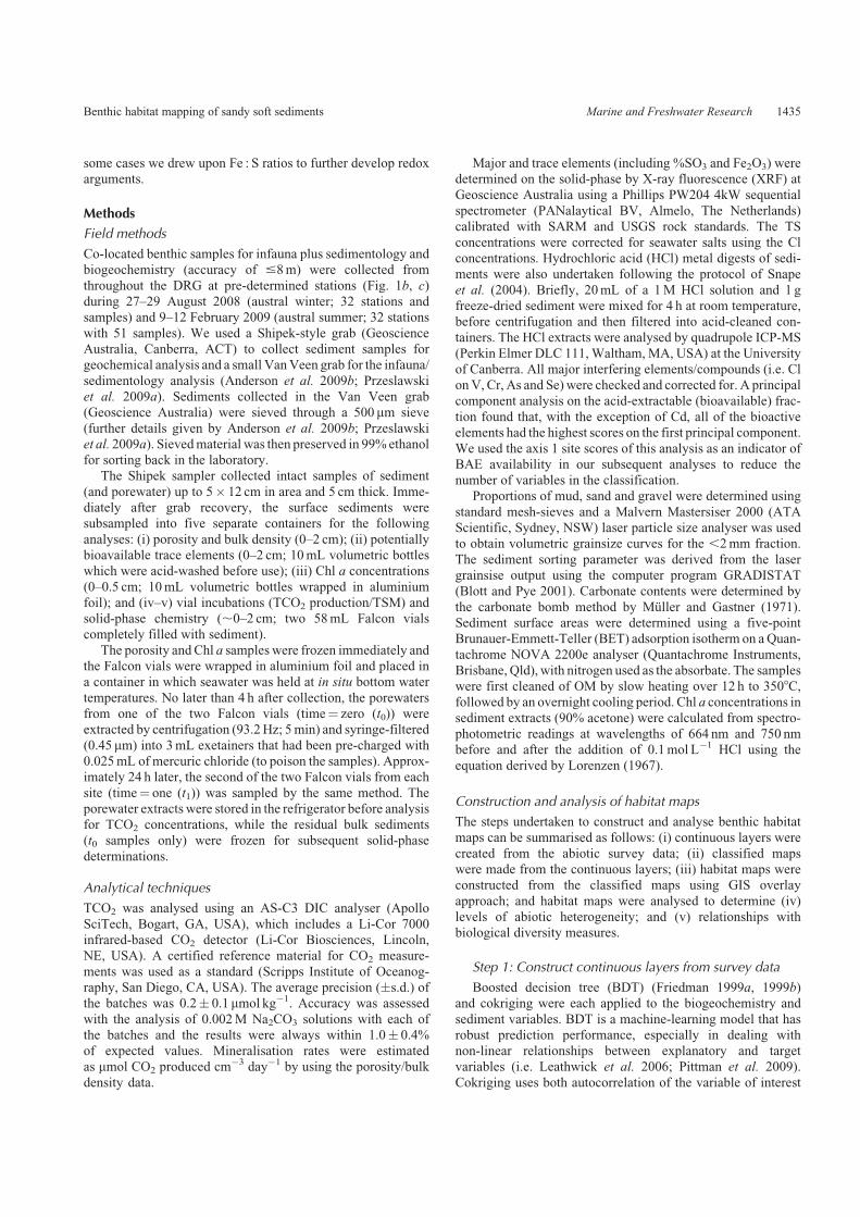
Focal variety analysis

The FVA (Fig. 7) incorporated all patch types irrespective of thecell count and reflected the patch type diversity evident inthe combined maps (Fig. 6). The most heterogeneous sediments

were observed in the polychaete hummocks in February. Localhotspots of heterogeneity were also observed in August in thevicinity of the 20m isobath.

Relationships between habitat classifications and biologicaldiversity measures

Species richness of ostracods and cumaceans was generallyhigher in February (10� 2.9 per station, �s.d.) than August

(5.1� 3.3 per station) and correlated with Shannon–Wienerdiversity in both seasons (Fig. 8a). Stations 3, 61, 70, 71, 76 and80 deviated from the main February trends in the species rich-

ness versus Shannon–Wiener diversity and Pielou’s evennesscross-plots (Fig. 8a, b). Five of these stations were situated in thedrift algae zone and had molar S : Fe ratios between one and two

Other classes

1: Low Chl a, Low TSM, Low TS, Mod BAE on moderately sorted calcareous silica sand bottom

Other classes

2: Low Chl a, Low TSM, Low TS, Low BAE on moderately sorted calcareous silica sand bottom

80: Mod Chl a, Low TSM, Low TS, High BAE on poorly sorted calcareous silica sand bottom

77: Low Chl a, Low TSM, Low TS, High BAE on poorly sorted calcareous silica sand bottom

63: Mod Chl a, Low TSM, Low TS, Mod BAE on poorly sorted calcareous silica sand bottom

58: Low Chl a, Low TSM, Mod TS, Mod BAE on poorly sorted calcareous silica sand bottom54: Low Chl a, Mod TSM, Low TS, Mod BAE on poorly sorted calcareous silica sand bottom

51: Low Chl a, Low TSM, Low TS, Mod BAE on poorly sorted calcareous silica sand bottom31: Low Chl a, Low TSM, Low TS, Mod BAE on poorly sorted calcareous silica muddy sand bottom

28: Low Chl a, Low TSM, Mod TS, Mod BAE on poorly sorted calcareous silica muddy sand bottom

15: Mod Chl a, Low TSM, Low TS, Mod BAE on moderately sorted calcareous silica sand bottom



3: Low Chl a, Low TSM, Mod TS, Low BAE on moderately sorted calcareous silica sand bottom

5: Low Chl a, Mod TSM, Low TS, Low BAE on moderately sorted calcareous silica sand bottom

6: Low Chl a, Mod TSM, Low TS, Mod BAE on moderately sorted calcareous silica sand bottom

7: Low Chl a, Mod TSM, Mod TS, Low BAE on moderately sorted calcareous silica sand bottom

8: Low Chl a, Low TSM, Mod TS, Mod BAE on moderately sorted calcareous silica sand bottom10: Low Chl a, Mod TSM, Mod TS, Mod BAE on moderately sorted calcareous silica sand bottom

12: Mod Chl a, Mod TSM, Mod TS, Mod BAE on moderately sorted calcareous silica sand bottom

21: Low Chl a, Low TSM, Low TS, Low BAE on moderately sorted silica sand bottom

22: Low Chl a, Mod TSM, Low TS, Low BAE on moderately sorted silica sand bottom23: Low Chl a, Mod TSM, Mod TS, Low BAE on moderately sorted silica sand bottom

27: Low Chl a, Mod TSM, Mod TS, Mod BAE on poorly sorted calcareous silica muddy sand bottom

34: Low Chl a, Low TSM, High TS, Mod BAE on poorly sorted calcareous silica muddy sand bottom

57: Low Chl a, Mod TSM, Mod TS, Mod BAE on poorly sorted calcareous silica sand bottom

58: Low Chl a, Low TSM, Mod TS, Mod BAE on poorly sorted calcareous silica sand bottom60: Mod Chl a, Mod TSM, Mod TS, Mod BAE on poorly sorted calcareous silica sand bottom

35: Low Chl a, Mod TSM, High TS, Mod BAE on poorly sorted calcareous silica muddy sand bottom


(a)

(b)

Fig. 6. Combined sediment–biogeochemistry habitat maps for (a) August and (b) February. Themaps have overlays which show the 15, 20 and 25m isobaths

and habitats identified in towed-video (CSIRO 1993). Abbreviations are: Chl a, chlorophyll a; TSM, total sediment metabolism; TS, total sulfur; BAE,

bioactive elements.


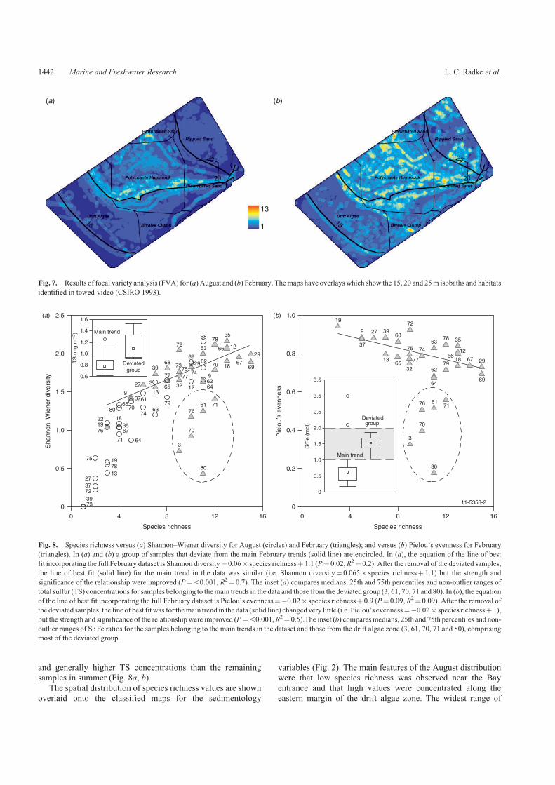
and generally higher TS concentrations than the remainingsamples in summer (Fig. 8a, b).

The spatial distribution of species richness values are shownoverlaid onto the classified maps for the sedimentology

variables (Fig. 2). The main features of the August distributionwere that low species richness was observed near the Bay

entrance and that high values were concentrated along theeastern margin of the drift algae zone. The widest range of

(a) (b)

13

1

Fig. 7. Results of focal variety analysis (FVA) for (a) August and (b) February. Themaps have overlays which show the 15, 20 and 25m isobaths and habitats

identified in towed-video (CSIRO 1993).

2.5

0

0.5

1.0

1.5

2.0

0 4 8

Species richness

12 16

80

3

70

7663

64

716179

35

1266

1879 67

29

69

7868

63

62

72

32

77

12

96264

74

2969

757368

77

6513

3

39

27

61

74

7339723727

13781975

71

6735

1832

6680 70

379

1976

0.6

0.8

1.0

1.2

1.4

1.6

Sha

nnon

–Wie

ner

dive

rsity

(a)

Main trend

Deviatedgroup

0 4 8 12 16

0

0.2

0.4

0.6

0.8

1.0(b)

Species richness

Pie

lou’

s ev

enne

ss

19

37

27 3968

13

729

75

32

77

74

6378 35

1266

1879

62

64

67 29

69

716176

65

3

80

70

3.5

0

0.5

1.0

1.5

2.0

2.5

3.5

S/F

e (m

ol)

11-5353-2

Main trend

Deviatedgroup

TS

(m

g m

�2 )

Fig. 8. Species richness versus (a) Shannon–Wiener diversity for August (circles) and February (triangles); and versus (b) Pielou’s evenness for February

(triangles). In (a) and (b) a group of samples that deviate from the main February trends (solid line) are encircled. In (a), the equation of the line of best

fit incorporating the full February dataset is Shannon diversity¼ 0.06� species richnessþ 1.1 (P¼ 0.02,R2¼ 0.2). After the removal of the deviated samples,

the line of best fit (solid line) for the main trend in the data was similar (i.e. Shannon diversity¼ 0.065� species richnessþ 1.1) but the strength and

significance of the relationship were improved (P¼,0.001, R2¼ 0.7). The inset (a) compares medians, 25th and 75th percentiles and non-outlier ranges of

total sulfur (TS) concentrations for samples belonging to themain trends in the data and those from the deviated group (3, 61, 70, 71 and 80). In (b), the equation

of the line of best fit incorporating the full February dataset is Pielou’s evenness¼�0.02� species richnessþ 0.9 (P¼ 0.09, R2¼ 0.09). After the removal of

the deviated samples, the line of best fit was for themain trend in the data (solid line) changed very little (i.e. Pielou’s evenness¼�0.02� species richnessþ 1),

but the strength and significance of the relationship were improved (P¼,0.001,R2¼ 0.5).The inset (b) comparesmedians, 25th and 75th percentiles and non-

outlier ranges of S : Fe ratios for the samples belonging to the main trends in the dataset and those from the drift algae zone (3, 61, 70, 71 and 80), comprising

most of the deviated group.


species richness was observed in the polychaete hummocks inAugust, with the lowest values occurring in the vicinity of the20m isobath. There was no obvious spatial pattern in species

richness in February, although there were still some locally lowvalues near the 20m isobath.

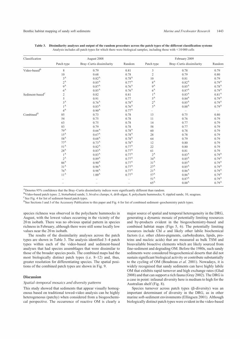
The results of the dissimilarity analyses across the patchtypes are shown in Table 3. The analysis identified 3–4 patch

types within each of the video-based and sediment-basedanalyses that had species assemblages that were dissimilar tothose of the broader species pools. The combined maps had the

most biologically distinct patch types (i.e. 8–12) and, thus,greater resolution for differentiating species. The spatial posi-tions of the combined patch types are shown in Fig. 9.

Discussion

Spatial–temporal mosaics and diversity patterns

This study showed that sediments that appear visually homog-enous based on traditional towed-video analysis can be highlyheterogeneous (patchy) when considered from a biogeochemi-

cal perspective. The occurrence of reactive OM is clearly a

major source of spatial and temporal heterogeneity in the DRG,generating a dynamic mosaic of potentially limiting resourcesand by-products evident in the biogeochemistry-based and

combined habitat maps (Figs 5, 6). The potentially limitingresources include Chl a and likely other labile biochemicalfactors (i.e. other chloro-pigments, carbohydrates, lipids, pro-teins and nucleic acids) that are measured as bulk TSM and

bioavailable bioactive elements which are likely sourced fromfine-sediment and degrading OM. Before the 1980s, such sandysediments were considered biogeochemical deserts that did not

sustain significant biological activity or contribute substantiallyto the cycling of OM (Boudreau et al. 2001). Nowadays, it iswidely recognised that sandy sediments can have highly labile

OM that exhibits rapid turnover and high exchange rates (Glud2008) and that can support a rich fauna (Gray 2002). TheDRG isa case in point: infaunal diversity here is medium to high for theAustralian shelf (Fig. 8).

Species turnover across patch types (b-diversity) was animportant determinant of diversity in the DRG, as in othermarine soft-sediment environments (Ellingsen 2001). Although

biologically distinct patch types were evident in the video-based

Table 3. Dissimilarity analyses and output of the random procedure across the patch types of the different classification systems

Analysis includes all patch types for which there were biological samples, including those with ,10 000 cells

Classification August 2008 February 2009

Patch type Bray–Curtis dissimilarity Random Patch type Bray–Curtis dissimilarity Random

Video-basedB 8 0.79 0.81 3 0.78 0.79

10 0.68 0.78 2 0.79 0.80

3A 0.82A 0.78A 10 0.81 0.79

2A 0.85A 0.77A 8A 0.82A 0.79A

9A 0.87A 0.76A 9A 0.85A 0.78A

6A 0.85A 0.76A 6A 0.87A 0.79A

Sediment-basedC 2 0.82 0.81 1A 0.83A 0.81A

5 0.91 0.77 5A 0.84A 0.79A

3A 0.76A 0.78A 2A 0.85A 0.79A

1A 0.83A 0.76A 3A 0.88A 0.79A

4A 0.90A 0.77A – – –

CombinedD 85 0.73 0.78 13 0.75 0.80

54 0.75 0.78 11 0.76 0.79

63 0.75 0.78 14 0.77 0.79

83 0.79 0.78 58 0.77 0.79

79A 0.66A 0.78A 60 0.78 0.79

15A 0.67A 0.78A 28 0.78 0.79

58A 0.68A 0.78A 64 0.79 0.79

77A 0.73A 0.78A 12 0.80 0.79

51A 0.82A 0.77A 22 0.80 0.79

28A 0.83A 0.77A 61 0.81 0.79

1A 0.83A 0.77A 2A 0.83A 0.79A

2A 0.89A 0.77A 34A 0.85A 0.79A

86A 0.90A 0.77A 31A 0.85A 0.79A

31A 0.96A 0.77A 27A 0.85A 0.79A

76A 0.98A 0.77A 21A 0.86A 0.79A

11A 1.00A 0.77A 57A 0.86A 0.79A

– – – 51A 0.87A 0.79A

– – – 65A 0.88A 0.79A

ADenotes 95% confidence that the Bray–Curtis dissimilarity indices were significantly different than random.BVideo-based patch types: 2, bioturbated sands; 3, bivalve clumps; 6, drift-algae; 8, polychaete hummocks; 9, rippled sands; 10, seagrass.CSee Fig. 4 for list of sediment-based patch types.DSee Sections I and J of the Accessory Publication to this paper and Fig. 6 for list of combined sediment–geochemistry patch types.


and sediment-based classification systems, the combined mapsincorporating biogeochemical data contained more biologically

relevant information (Table 3). The pattern that has emergedfrom the generalised dissimilarity analysis (Fig. 9) is that therewas a good spatial coverage of biologically-relevant patchtypes across the DRG. This is with the exception of parts of

the bioturbated sands and polychaete hummocks where patchdiversity was strongly controlled by bioturbation.

Mounds built by polychaetes comprised the most heteroge-

neous sediment in the dataset (Fig. 7). Burrows/tubes causesediment heterogeneity in several ways: (i) feeding, tube con-struction and burrowing cause the continuous translocation of

materials between reaction zones; (ii) bioirrigation of burrows/tubes introduces oxygenated water into sediment (Przeslawskiet al. 2009b); and (iii) new labile OM (i.e. mucoid secretions) isintroduced into sediment by organisms (Kristensen 2000). The

labile materials form substrates for bacteria. This is also apotential source of microbial patchiness to which infauna areknown to respond (Gray 2002). Moreover, even relict burrows,

which can persist for years, function as passive irrigators(Munksby et al. 2002) and traps for reactive OM (includingphytoplankton debris) producing hot-spots of biological activity

and decomposition (Ray and Aller 1985; Aller and Aller 1986).Most fundamentally, polychaete tubes increase the area of

anoxic–oxic interface (Glud 2008) and this is apparent in themixture of moderate and low TS concentrations in the poly-chaete mounds in February (Fig. 3b).

Although dense aggregations of polychaete tubes can

stabilise seafloor sediments by altering the characteristics ofnear-bed flow (Eckman et al. 1981), the lateral extentof polychaete tube-building activity in the DRG was likely

constrained by hydrodynamic processes occurring near theBay entrance and landward of the 20m isobath. The area ofrippled sands near the entrance (patch types 1–2; Figs 6, 9) forms

part of the central corridor of energy which extends towards thenorth-north-west in the Bay (M. Hughes, personal communica-tion). These sands are otherwise distinguished in being the mostresource-poor sediments in the DRG because the high wave-

energy reduces the amount of fine-sediment and OM that cansettle. As swell waves propagate through the Bay, they shoal andwave-induced flows at the bottom become more energetic

and more able to mobilise sediments. At water depths ,20m,benthic sandy sediments can experience significant reworkingby waves under modal wave conditions (M. Hughes, personal

Other classes


Other classes(a)

(b)

11: Mod Chl a, Mod TSM, Low TS, Mod BAE on moderately sorted calcareous silica sand bottom


79: Mod Chl a, Low TSM, Low TS, High BAE on Moderately sorted calcareous silica sand bottom

86: Low Chl a, Low TSM, Low TS, Mod BAE on poorly sorted silica sand bottom

77: Low Chl a, Low TSM, Low TS, High BAE on poorly sorted calcareous silica sand bottom

76: Low Chl a, Mod TSM, Low TS, High BAE on poorly sorted calcareous silica sand bottom

58: Low Chl a, Low TSM, Mod TS, Mod BAE on poorly sorted calcareous silica sand bottom

51: Low Chl a, Low TSM, Low TS, Mod BAE on poorly sorted calcareous silica sand bottom

31: Low Chl a, Low TSM, Low TS, Mod BAE on poorly sorted calcareous silica muddy sand bottom

15: Mod Chl a, Low TSM, Low TS, Mod BAE on moderately sorted calcareous silica sand bottom



21: Low Chl a, Low TSM, Low TS, Low BAE on moderately sorted silica sand bottom

27: Low Chl a, Mod TSM, Mod TS, Mod BAE on poorly sorted calcareous silica muddy sand bottom

31: Low Chl a, Low TSM, Low TS, Mod BAE on poorly sorted calcareous silica muddy sand bottom

34: Low Chl a, Low TSM, High TS, Mod BAE on poorly sorted calcareous silica muddy sand bottom

51: Low Chl a, Low TSM, Low TS, Mod BAE on poorly sorted calcareous silica sand bottom57: Low Chl a, Mod TSM, Mod TS, Mod BAE on poorly sorted calcareous silica sand bottom

65: Low Chl a, Mod TSM, Low TS, Mod BAE on poorly sorted calcareous silica sand bottom

Fig. 9. Combined sediment–biogeochemistry habitat maps for (a) August and (b) February including only those patch types where discrimination

was observed in the dissimilarity analyses across the patch types (Table 3). The maps have overlays which show the 15, 20 and 25m isobaths and

habitats identified in towed-video (CSIRO 1993). Abbreviations are: Chl a, chlorophyll a; TSM, total sediment metabolism; TS, total sulfur; BAE, bioactive

elements.


communication). Such energetic environments are expected tosupport specialised and low diversity faunas (Gray 2002) and

this is consistent with our results. There was good biologicaldiscrimination for patch types in the western part of the Bay,where drift algae settles and in the rippled sands near the

entrance (Fig. 9). Moreover, sediment patch type 1 foundextensively in the eastern part of the Bay (Fig. 4) had statisticallyfewer species than sediment patch type 5 (see Section D(c) of

the Accessory Publication to this paper).

Patterns of diversity in relation to reactive carbonconcentrations

Available food resources may set a limit on the number ofspecies that can occur in the DRG during certain times of the

year (i.e. winter) because the average number of species perstation and overall species numbers were higher during thesummer survey (Fig. 8a, b) when there was apparently more

reactive OM in the sediments (0.9 kmol C in February comparedwith 0.4 kmol C inAugust; calculated fromFig. 3e, f ). Althoughit is acknowledged that ex situ incubation will likely biasdegradation rates of sandy sediments (Boudreau et al. 2001),

TS concentrations were also approximately twice as high inFebruary (Fig. 3b). The higher TS concentrations point tohigher reactive carbon concentrations because this is the major

factor controlling bacterial sulfate reduction rates (Berner1984). Moreover, the higher February TS concentrations mayexplain the lower bioavailable bioactive element concentrations

at this time (Fig. 3h), because these elements cannot be extractedwith 1M HCl when sequestered by pyrite (Snape et al. 2004).

Although station-specific species diversity (a-diversity) andpatch-diversity were higher in February, b-diversity was lowerat this time. There were fewer biologically-relevant patches inFebruary compared with August (Table 3). Patches initiatedby temporal events (such as food input) promote a diversity

because species assemblages can exist at different stages ofcolonisation and succession (Grassle and Maciolek 1992). TheFebruary decline in b-diversity might then be explained by

greater mobility of species across the patch types to fostercolonisation, as well as less competition for more abundantsummer resources. However, large amounts of potentially

limiting resources are also known to reduce niche dimension-ality and when supply is constant, may be conducive tomonopolisation of resources by relatively few competitivespecies (Harpole and Tilman 2007).

Chl a concentrations and TSM were relatively high in thevicinity of the 20m isobath (Fig. 3c–f ), yet this part of the DRGsupported a low diversity cumacean/ostracod fauna in August.

The average winter species richness (�s.d.) of samples with themoderate TSM levels (i.e. situated along the 20m isobath) was2� 1.6 compared with 5.7� 3.2 for the rest of DRGwhere TSM

was lower (Fig. 3e). This result may be explained by competitiveexclusion by the mound-building species Mesochaetopterus

minutus during winter when food resources were in shorter

supply elsewhere in the DRG. The higher Chl a concentrationsand TSM in this region may relate to the formation of mucus-bacteria complexes (see above) and the occurrence of benthicalgae. Incorporation of phytoplankton into sediment may also

increase over polychaete mounds because the interaction

between micro-topography and flow can reduce benthic shearstress (Ramey and Bodnar 2008).

Influence of sediment anoxia on local diversity patterns

Sediment anoxia is a likely explanation for the lower Pielou’sevenness values (and, hence, Shannon–Wiener diversity

indices) in samples 3, 61, 70, 71 and 80 from the western DRG(Fig. 8a, b). February TS concentrations of these samples weregenerally high for the DRG and the average molar TS : Fe ratioswere between those of FeS2 and FeS (i.e. 1.4� 0.4 compared

with 0.6� 0.3 for other samples in theDRG), which are the solidphase products of sulfate reduction (Fig. 8a, b). The circulationof the Bay pushes macroalgal wrack (and fine sediment) into the

western DRGwhere its presence, when abundant, may suppresssediment resuspension. Anoxia is caused by algal breakdownand by a reduction in the turbulent transfer of oxygen to the

sediment under the algal wrack. These results provide anevidence-base to support Langtry and Jacoby’s (1996) hypoth-esis that low interstitial oxygen concentrations were the cause

of low fish and decapod species richness in Jervis Bay algalwracks. These results also highlight that Shannon–Weinerdiversity and species richness measures can respond differentlyto local-scale environmental stresses as suggested by Scrosati

and Heaven (2007).

Strengths and limitations

The mapping approach undertaken in this study had certain

limitations that are difficult to quantify and it is not intended toreplace direct quantification of biodiversity (if this is possible).The classifications were arbitrary and some information was

undoubtedly lost in the processes of splitting data ranges andcombining patches. Moreover, exploratory variables such asbioavailable bioactive elements were given equal weighting tovariables of established biological importance (i.e. Chl a;

Tselepides et al. 2000). As with many studies on infaunaldiversity, the sieve size used here precluded collection of smallostracods and cumaceans. As such, the richness and abundance

of these taxa may be underestimated (Wilson 2006). Moreover,in our ‘surrogacy’ approach, maps were made before analysesthat could identify the best abiotic drivers of species in the

dataset.Despite the stated limitations, the incorporation of biogeo-

chemical factors and consideration of time as a variable inbenthic habitat maps provided a better framework for differen-

tiating species and interpreting infaunal diversity patterns thanmaps from individual studies based solely on physical sedimen-tology or video-analysis (Table 3), which are more commonly

used as biodiversity surrogates. Classifiedmaps based on abioticsurrogates are usually used in marine environmental manage-ment to fill gaps where biological data are lacking, in order to

identify regions where biodiversity conservation may bemaximised (Department of Environment and Heritage 2005;Harris et al. 2008). The results of this study suggest that simple

measures of carbon reactivity and redox (which vary temporally)can add significant value to such maps.

This study brings into question the delineation of habitatsbased on video assessments because only two of the video-based

‘habitats’ (i.e. drift algae and rippled sands) were biologically


relevant across the months (Table 3). Thus, from a broaderperspective, biogeochemistry and time can inform environmen-

tal management by highlighting the dynamic nature of marinesystems and the inclusion of these variables in mapping studiesprovides an opportunity to better define ‘habitats’ (biologically-

distinguished patches) from amongst a dynamic array of patchtypes. This is particularly true in accessible near-shore areas(including coastal MPAs), where it may be feasible to acquire

temporal datasets. Such studies would benefit from analyseswhich identify the most biologically-relevant variables beforeproceeding to map construction.

Acknowledgements

This research forms part of the Surrogates Program in the Commonwealth

Environmental Research Facilities (CERF) Marine Biodiversity Hub

(administered through the Australian Government’s Department of

Sustainability, Environment, Water, Population and Communities).

S. Corson,M. Carey, J. Jaycock, P. Harris,M.Hughes, J. Smith andA. Potter

provided field support. T. Watson, J. Trafford, B. Poignand, K. Wall,

J. Chen, F. Krykowa and L. Webber undertook laboratory analyses.

S. Nichol provided GRADISTAT output for the sediment analyses,

M. Hughes and T. Whiteway participated in helpful discussions, A. Syme

(Museum Victoria) and L. Hughes (Australian Museum) helped with

taxonomy and S. Foster (CSIRO Marine) provided crucial feedback on the

new statistical technique developed for this study. The manuscript was

improved thanks to constructive reviews by P. Harris, N. Bax, P. Herman,

A. Boulton and two anonymous reviewers. This manuscript is published

with permission of the CEO, Geoscience Australia.

References

Aller, J. Y., and Aller, R. C. (1986). Evidence for localised enhancement

of biological activity associated with tube and burrow structures in

deep-sea sediments at the HEBBLE site, western North Atlantic. Deep-

sea Research. Part I, Oceanographic Research Papers 33, 755–790.

doi:10.1016/0198-0149(86)90088-9

Anderson, T. J., Syms, C., Roberts, D. A., and Howard, D. F. (2009a).

Multiscale fish-habitat associations and the use of habitat surrogates to

predict the organisation and abundance of deep-water fish assemblages.

Journal of Experimental Marine Biology and Ecology 379, 34–42.

doi:10.1016/J.JEMBE.2009.07.033

Anderson, T., Brooke, B., Radke, L., McArthur, M., and Hughes, M.

(2009b). Mapping and characterising soft-sediment habitats and evalu-

ating physical variables as surrogates of biodiversity in Jervis Bay,

NSW. Geoscience Australia Record 2009/10. Geoscience Australia,

Canberra.

Berner, R. A. (1984). Sedimentary pyrite formation: an update.Geochimica

etCosmochimicaActa48, 605–615. doi:10.1016/0016-7037(84)90089-9

Blott, S. J., and Pye, K. (2001). Gradistat: a grain size distribution and

statistics package for the analysis of unconsolidated sediments. Earth

Surface Processes and Landforms 26, 1237–1248. doi:10.1002/ESP.261

Boudreau, B. P., Huettel, M., Forster, S., Jahnke, R. A., McLachlan, A.,

Middleburg, J. J., Nielsen, P., Sansone, F., Taghon,G.,VanRaaphorst,W.,

Webster, I., Weslawski, J. M., Wiberg, P., and Sundby, P. (2001).

Permeable marine sediments: overturning an old paradigm. Eos, Trans-

actions, American Geophysical Union 82, 133–136.

Clarke, K. R., andWarwick, R.M. (2001). ‘Change inMarine Communities:

an Approach to Statistical Analysis and Interpretation.’ 2nd edn.

(Primer-E: Plymouth, UK.)

Cohen, A. C., Peterson, D. E., and Maddocks, R. F. (2007). Ostracoda. In

‘The Light and Smith Manual: Intertidal Invertebrates from Central

California to Oregon’. (Ed. J. T. Carlton.) pp. 417–446. (University of

California Press: Berkeley, CA.)

Cook, P. L. M., Wenzhofer, F., Glud, R. N., Janssen, F., and Huettel, M.

(2007). Benthic solute exchange and carbon mineralisation in two

shallow subtidal sandy sediments: effect of advective pore-water

exchange. Limnology and Oceanography 52, 1943–1963. doi:10.4319/

LO.2007.52.5.1943

CSIRO (1993). Jervis Bay Marine Ecological Studies Final Report. CSIRO

Division of Fisheries, Jervis Bay, NSW.

De’ath, G., and Fabricius, K. E. (2000). Classification and regression trees:

a powerful yet simple technique for ecological data analysis Ecology

81, 3178–3192. doi:10.1890/0012-9658(2000)081[3178:CARTAP]

2.0.CO;2

Department of Environment and Heritage (2005). National marine biore-

gionalisation of Australia. Compilation DVD. Commonwealth of

Australia, Canberra.

Eckman, J. E., Nowell, A. R. M., and Jumars, P. A. (1981). Sediment

destabilisation by animal tubes. Journal of Marine Research 39,

361–374.

Ellingsen, K. E. (2001). Biodiversity of a continental shelf soft-sediment

macrobenthos community. Marine Ecology Progress Series 218, 1–15.

doi:10.3354/MEPS218001

Emerson, S., and Hedges, J. (2003). Sediment diagenesis and benthic fluxes.

In ‘Treatise on Geochemistry’. (Eds H. D. Holland and K. K. Turekian.)

pp. 293–319. (Elsevier Pergamon: Oxford.)

Emery, K. O. (1968). Relict sediments on continental shelves of the world.

The American Association of Petroleum Geologists Bulletin 52,

445–464.

Ersahin, S. (2003). Comparing ordinary kriging and cokriging to estimate

infiltration rate. Soil Science Society of America Journal 67, 1848–1855.

doi:10.2136/SSSAJ2003.1848

Folk, R. L. (1980). ‘Petrology of Sedimentary Rocks.’ (Hemphill Publish-

ing: Cedar Hill, TX.)

Franke, U., Polerecky, L., Precht, E., and Huettal, M. (2006). Wave tank

study of particulate organic matter degradation in permeable sediments.

Limnology and Oceanography 51, 1084–1096. doi:10.4319/LO.2006.

51.2.1084

Friedman, J. H. (1999a). Greedy function approximation: a gradient boost-

ing machine. Department of Statistics, Stanford University, Technical

Report, San Francisco, CA.

Friedman, J. H. (1999b). Stochastic gradient boosting. Department of

Statistics, Stanford University, Technical Report, San Francisco, CA.

Glud, R. N. (2008). Oxygen dynamics of marine sediments.Marine Biology

Research 4, 243–289. doi:10.1080/17451000801888726

Gogina, M., Glockzin, M., and Zettler, M. L. (2010). Distribution of benthic

macrofaunal communities in the western Baltic Sea with regard to near-

bottom environmental parameters. 1. Causal analysis. Journal of Marine

Systems 79, 112–123. doi:10.1016/J.JMARSYS.2009.07.006

Grassle, J. F., and Maciolek, N. J. (1992). Deep-sea richness: regional and

local diversity estimates from quantitative bottom samples. American

Naturalist 139, 313–341. doi:10.1086/285329

Gray, J. S. (2002). Species richness of marine soft sediments. Marine

Ecology Progress Series 244, 285–297. doi:10.3354/MEPS244285

Harpole,W. S., and Tilman, D. (2007). Grassland species loss resulting from

reduced niche dimension. Nature 446, 791–793. doi:10.1038/

NATURE05684

Harris, P. T., and Whiteway, T. (2009). High seas marine protected areas:

benthic environmental conservation priorities from GIS analysis of

global ocean biophysical data. Ocean and Coastal Management 52,

22–38. doi:10.1016/J.OCECOAMAN.2008.09.009

Harris, P. T., Heap, A. D., Whiteway, T., and Post, A. (2008). Application

of biophysical information to support Australia’s representative

protected area program. Ocean and Coastal Management 51, 701–711.

doi:10.1016/J.OCECOAMAN.2008.07.007

Heap, A., Bryce, S., Ryan, D., Radke, L., Smith, C., Harris, P., and Heggie, D.

(2001). Australian estuaries and coastal waterways: a geoscience


perspective for improved and integrated resource management. A report

to the National Land and Water Resources Audit Theme 7: Ecosystem

Health. AGSO Record 2001/07, Canberra.

Holloway, P. E., Symonds, G., and Nunes Vaz, R. (1992). Observations of

circulation and exchange processes in Jervis Bay, New South Wales.

Australian Journal of Marine and Freshwater Research 43, 1487–1515.

doi:10.1071/MF9921487

Huang, Z., Nichol, S., Daniell, J., Siwabessy, J., and Brooke, B. (2009).

Predictive modelling of seabed sediment parameters using multibeam

acoustic data: a case study on the Carnarvon Shelf,Western Australia. In

‘Proceedings of the 10th International Conference onGeoComputation’.

(Eds B.G. Lees and S.W. Laffan.) pp. 114–119. (UNSWPress: Sydney.)

Huang, Z., Brooke, B., and Harris, P. T. (2011). A new approach to mapping

marine benthic habitats using physical environmental data. Continental

Shelf Research 31, S4–S16. doi:10.1016/J.CSR.2010.03.012

Janssen, F., Huettel, M., and Witte, U. (2005). Pore-water advection and

solute fluxes in permeable marine sediments (II): benthic respiration at

three sandy sites with different permeabilities (German Bight, North

Sea). Limnology and Oceanography 50, 779–792. doi:10.4319/

LO.2005.50.3.0779

Kelaher, B. P., and Levington, J. S. (2003). Variation in detrital enrichment

causes spatio-temporal variation in soft-sediment assemblages. Marine


Kirk, J. T. O. (1994). ‘Light and Photosynthesis in Aquatic Systems.’

(Cambridge University Press: Cambridge, UK.)

Kristensen, E. (2000). Organic matter diagensis at the oxic/anoxic interface

in coastal marine sediments, with emphasis on the role of burrowing

animals. Hydrobiologia 426, 1–24. doi:10.1023/A:1003980226194

Langtry, S. K., and Jacoby, C. A. (1996). Fish and decapod crustaceans

inhabiting drifting algae in Jervis Bay, New South Wales. Australian

Journal of Ecology 21, 264–271. doi:10.1111/J.1442-9993.1996.

TB00608.X

Leathwick, J. R., Elith, J., Francis, M. P., Hastie, T., and Taylor, P. (2006).

Variation in demersal fish species richness in the oceans surrounding

New Zealand: an analysis using boosted regression trees. Marine


Leecaster, M. (2003). Spatial analysis of grain size in Santa Monica Bay.

Marine Environmental Research 56, 67–78. doi:10.1016/S0141-1136

(02)00325-2

Lorenzen, C. J. (1967). Determination of chlorophyll and pheopigments:

spectrophotometric equations. Limnology and Oceanography 12,

343–346. doi:10.4319/LO.1967.12.2.0343

NSW Marine Parks Authority (2010). Seabed mapping in the Solitary

Islands and Jervis Bay Marine Park. NSW Marine Parks Authority,

Hurstville, NSW.

McArthur,M.A., Brooke, B. P., Przeslawski, R., Ryan,D.A., Lucieer, V. L.,

Nichol, S., McCallum, A. W., Mellin, C., Cresswell, I. D., and Radke,

L. C. (2010). On the use of abiotic surrogates to describe marine

benthic biodiversity. Estuarine, Coastal and Shelf Science 88, 21–32.

doi:10.1016/J.ECSS.2010.03.003

Muller, G., andGastner,M. (1971). The ‘karonatebombe’ a simple device for

the determination of the carbonate content in sediments, soils and other

materials. Neues Jahrbuch fur Mineralogie-Monatshefte 10, 466–469.

Munksby, N., Benthien, M., and Glud, R. N. (2002). Flow-induced flushing

of relict tube structures in the central Skagerrak (Norway). Marine

Biology 141, 939–945. doi:10.1007/S00227-002-0874-X

Pittman, S. J., Costa, B. M., and Battista, T. A. (2009). Using Lidar

bathymetry and boosted regression trees to predict the diversity

and abundance of fish and corals. Journal of Coastal Research SI(53),

27–38. doi:10.2112/SI53-004.1

Poulos, H. G. (1988). ‘Marine Geotechnics.’ (Unwin Hyman: London.)

Przeslawski, R., Radke, L., and Hughes, M. (2009a). Temporal and fine-

scale variation in the biogeochemistry of Jervis Bay. Geoscience

Australia, Record 2009/12. Geoscience Australia, Canberra.

Przeslawski, R., Zhu,Q., andAller, R. C. (2009b). Effects of abiotic stressors

on infaunal burrowing and associated sediment characteristics. Marine


Przeslawski, R., Currie, D. R., Sorokin, S. J., Ward, T. M., Althaus, F., and

Williams, A. (2011). Utility of a spatial habitat classification system as a

surrogate of marine benthic community structure for the Australian

margin. ICES Journal of Marine Science 68, 1954–1962. doi:10.1093/

ICESJMS/FSR106

Radke, L. C., Heap, A. D., Douglas, G., Nichol, S., Trafford, J., Li, J., and

Przeslawski, R. (2011). A geochemical characterization of deep-sea

floor sediments of the northern Lord Howe Rise. Deep-sea Research.

Part II, Topical Studies in Oceanography 58, 909–921.

Ramey, P. A., and Bodnar, E. (2008). Selection by a deposit-feeding

polychaete, Polygordius jouinae, for sands with relatively high organic

content. Limnology and Oceanography 53, 1512–1520. doi:10.4319/

LO.2008.53.4.1512

Ray, A. J., and Aller, R. C. (1985). Physical irrigation of relict burrows:

implications for sediment chemistry. Marine Geology 62, 371–379.

doi:10.1016/0025-3227(85)90125-2

Scrosati, R., and Heaven, C. (2007). Spatial trends in community richness,

diversity and evenness across rocky intertidal environmental stress

gradients in eastern Canada. Marine Ecology Progress Series 342,

1–14. doi:10.3354/MEPS342001

Seiter, K., Hensen, C., Schroter, J., and Zabel, M. (2004). Organic carbon

content in surface sediments – defining regional provinces. Deep-sea

Research. Part I, Oceanographic Research Papers 51, 2001–2026.

doi:10.1016/J.DSR.2004.06.014

Snape, I., Scouller, R. C., Stark, S. C., Stark, J., Riddle,M. J., andGore, D. B.

(2004). Characterisation of the dilute HCl extraction method for the

identification of metal contamination in Antarctic marine sediment.

Chemosphere 57, 491–504. doi:10.1016/J.CHEMOSPHERE.2004.

05.042

Snelgrove, P. V. R. (1999). Getting to the bottom of marine biodiversity:

sedimentary habitats. Bioscience 49, 129–138. doi:10.2307/1313538

Sterner, R. W., and Hessen, D. O. (1994). Algal nutrient limitation and the

nutrition of aquatic herbivores. Annual Review of Ecology and System-

atics 25, 1–29. doi:10.1146/ANNUREV.ES.25.110194.000245

Stoddard, H. E., and Lowry, J. L. (2003). ‘Crustacea: Malacostraca:

Peracarida: Amphipoda, Cumacea, Mysidacea.’ (CSIRO Publishing:

Melbourne.)

Taylor, G. (1972). Sedimentation in Jervis Bay. Proceedings of the Linnean

Society of New South Wales 96, 297–306.

Thrush, S. F., Hewitt, J. E., Herman, P.M. J., andYsebaert, T. (2005).Multi-

scale analysis of species–environment relationships. Marine Ecology

Progress Series 302, 13–26. doi:10.3354/MEPS302013

Todd, B. J., and Greene, H. G. (2007). Mapping the seafloor for habitat

characterisation. Geological Association of Canada Special Paper 47,

Geological Association of Canada, St Johns, NL, Canada.

Tselepides,A., Polychronaki, T.,Marrale,D., Akoumianaki, I., Dell’Anno,A.,

Pusceddu, A., and Danavaro, R. (2000). Organic matter composition of

the continental shelf and bathyal sediments of the Cretan Sea

(NE Mediterrranean). Progress in Oceanography 46, 311–344.

doi:10.1016/S0079-6611(00)00024-0

Verfaillie, E., Du Four, I., Van Meirvenne, M., and Van Lancker, V. (2009).

Geostatistical modelling of sedimentological parameters using multi-

scale terrain variables: application along the Belgian part of the North

Sea. International Journal of Geographical Information Science 23,

135–150. doi:10.1080/13658810802184135

Wagai, R., andMayer, L. M. (2007). Sorptive stabilisation of organic matter

in soils by hydrous iron oxides. Geochimica et Cosmochimica Acta 71,

25–35. doi:10.1016/J.GCA.2006.08.047

Wilson, G. D. F. (2006). Arafura Sea biological survey. Report on RV

Southern Surveyor Expedition 05/2005, 28 April–28May 2005. Depart-

ment of the Environment and Heritage, Canberra.


Wu, C., Wu, J., Luo, Y., Zhang, L., and DeGloria, S. D. (2009). Spatial

estimation of soil total nitrogen using cokriging with predicted soil

organic matter content. Soil Science Society of America Journal 73,

1676–1681. doi:10.2136/SSSAJ2008.0205

Zacharias,M.A., andRoff, J.C. (2000). A hierarchical ecological approach to

conserving marine biodiversity. Conservation Biology 14, 1327–1334.

doi:10.1046/J.1523-1739.2000.99191.X

Zajac, R. N. (2008a). Macrobenthic biodiversity and sea floor landscape

structure. Journal of Experimental Marine Biology and Ecology 366,

198–203. doi:10.1016/J.JEMBE.2008.07.025

Zajac, R. N. (2008b). Challenges in marine soft-sediment benthoscape

ecology. Landscape Ecology 23, 7–18. doi:10.1007/S10980-007-

9140-4

Zonneveld, K. A. F., Versteegh, G. J. M., Kasten, S., Eglinton, T. I., Emeis,

K.-C., Huguet, C., Koch, B. P., de Lange, G. J., de Leeuw, J. W.,

Middleburg, J. J., Mollenhauer, G., Prahl, F. G., Rethemeyer, J., and

Wakeham, S. G. (2010). Selective preservation of organic matter in

marine environments: processes and impact on the sedimentary record.

Biogeosciences 7, 483–511. doi:10.5194/BG-7-483-2010

www.publish.csiro.au/journals/mfr


Documents

Including biogeochemical factors and a temporal component in benthic habitat maps: influences on infaunal diversity in a temperate embayment