Cleveland State University Cleveland State University

EngagedScholarship@CSU EngagedScholarship@CSU

ETD Archive

2012

In Vitro Biomechanical Testing and Computational: Modeling in In Vitro Biomechanical Testing and Computational: Modeling in

Spine Spine

Mageswaran Prasath Cleveland State University

Follow this and additional works at: https://engagedscholarship.csuohio.edu/etdarchive

Part of the Biomedical Engineering and Bioengineering Commons

How does access to this work benefit you? Let us know! How does access to this work benefit you? Let us know!

Recommended Citation Recommended Citation Prasath, Mageswaran, "In Vitro Biomechanical Testing and Computational: Modeling in Spine" (2012). ETD Archive. 248. https://engagedscholarship.csuohio.edu/etdarchive/248

This Dissertation is brought to you for free and open access by EngagedScholarship@CSU. It has been accepted for inclusion in ETD Archive by an authorized administrator of EngagedScholarship@CSU. For more information, please contact library.es@csuohio.edu.

IN VITRO BIOMECHANICAL TESTING AND COMPUTATIONAL

MODELING IN SPINE

MAGESWARAN PRASATH

BACHELOR OF ENGINEERING

University of Nigeria

May, 2001

MASTER OF ENGINEERING

University of North Carolina Chapel-Hill/North Carolina State University

Biomedical Engineering

May, 2005

Submitted in partial fulfillment of the requirements for the degree

DOCTOR OF ENGINEERING

Applied Biomedical Engineering

at the

CLEVELAND STATE UNIVERSITY

August, 2012

This dissertation has been approved for the

Department of Chemical and Biomedical Engineering

and the College of Graduate Studies by

Dr. R. McLain, Chairperson Department/Date

Dr. J. Gatica, Member Department/Date

Dr. S. Duffy, Member Department/Date

Dr. R. Setser, Member Department/Date

Dr. J. Lock, Member Department/Date

ACKNOWLEDGEMENTS

I would like to thank Dr. McLain for all his support and guidance

throughout my research. Thank you for taking the time to work with me and share

your experiences in research and life in general. I would also like to say thank

you to Dr. Benzel for his time, even with a busy schedule, he always made time,

his feedback and support was so valuable. I would also like to thank Dr.

Gilbertson for giving me the opportunity to take up spine research and for all his

help and guidance. To my committee members for their patience, flexibility and

advice, thank you for your support.

Many thanks and sincere gratitude to Robb Colbrunn and Tara Bonner for

their immense help and contribution, I wouldn’t have done it without your support.

Thank you for your time. I would like to also say thanks to Adam Bartsch and

Brian Perse for their encouragement and support.

Finally to my family and friends for all their love, encouragement and

support throughout my study.

v

IN VITRO BIOMECHANICAL TESTING AND COMPUTATIONAL

MODELING IN SPINE

MAGESWARAN PRASATH

ABSTRACT

Two separate in vitro biomechanical studies were conducted on human

cadaveric spines (Lumbar) to evaluate the stability following the implantation of

two different spinal fixation devices; interspinous fixation device (ISD) and Hybrid

dynamic stabilizers. ISD was evaluated as a stand-alone and in combination with

unilateral pedicle rod system. The results were compared against the gold

standard, spinal fusion (bilateral pedicle rod system). The second study involving

the hybrid dynamic system, evaluated the effect on adjacent levels using a hybrid

testing protocol. A robotic spine testing system was used to conduct the

biomechanical tests. This system has the ability to apply continuous

unconstrained pure moments while dynamically optimizing the motion path to

minimize off-axis loads during testing. Thus enabling precise control over the

loading and boundary conditions of the test. This ensures test reliability and

reproducibility.

We found that in flexion-extension, the ISD can provide lumbar stability

comparable to spinal fusion. However, it provides minimal rigidity in lateral

bending and axial rotation when used as a stand-alone. The ISD with a unilateral

pedicle rod system when compared to the spinal fusion construct were shown to

provide similar levels of stability in all directions, though the spinal fusion

construct showed a trend toward improved stiffness overall.

vi

The results for the dynamic stabilization system showed stability

characteristics similar to a solid all metal construct. Its addition to the supra

adjacent level (L3- L4) to the fusion (L4- L5) indeed protected the adjacent level

from excessive motion. However, it essentially transformed a 1 level into a 2 level

lumbar fusion with exponential transfer of motion to the fewer remaining discs

(excessive adjacent level motion).

The computational aspect of the study involved the development of a

spine model (single segment). The kinematic data from these biomechanical

studies (ISD study) was then used to validate a finite element model of the spine.

vii

TABLE OF CONTENTS

LIST OF TABLES ................................................................................................. xi

LIST OF FIGURES .............................................................................................. xii

CHAPTER OVERVIEW ....................................................................................... xv

CHAPTER

I. INTRODUCTION ....................................................................................... 1

II. BIOMECHANICAL TESTING OF SPINE ................................................... 4

2.1 Spinal Anatomy ............................................................................ 4

2.2 Biomechanical Role of the Intervertebral Disc ............................ 12

2.3 Spinal Ligaments ........................................................................ 13

2.4 Intervertebral Disc Degeneration ................................................ 14

2.5 Kinematic Parameters for Spine ................................................. 15

2.6 Multi-Segment Spine Testing .................................................... 17

2.6.1 Pure moment testing systems ........................................... 17

2.6.2 Follower load system ......................................................... 18

2.7 Specimen Preparation ................................................................. 19

2.8 Custom Spinal Test Fixtures ....................................................... 20

2.9 Follower Load Fixtures ................................................................ 24

2.10 Robotic Spine Testing ............................................................... 26

2.11 References ............................................................................... 29

III. PROPERTIES OF AN INTERSPINOUS FIXATION DEVICE (ISD) IN

LUMBAR FUSION CONSTRUCTS: A BIOMECHANICAL STUDY ......... 32

3.1 Abstract ....................................................................................... 32

3.1.1 Introduction ........................................................................ 32

viii

3.1.2 Methods ............................................................................. 33

3.1.3 Results .............................................................................. 33

3.1.4 Conclusions ....................................................................... 34

3.2 Introduction ................................................................................. 34

3.3 Methods ...................................................................................... 37

3.4 Surgical Treatment ...................................................................... 41

3.5 Results ........................................................................................ 42

3.6 Discussion ................................................................................... 46

3.7 Conclusions................................................................................. 50

3.8 References .................................................................................. 50

IV. HYBRID DYNAMIC STABILIZATION: A BIOMECHANICAL

ASSESSMENT OF ADJACENT AND SUPRA-ADJACENT LEVELS ...... 55

4.1 Abstract ....................................................................................... 55

4.1.1 Study design ...................................................................... 55

4.1.2 Summary of background ................................................... 55

4.1.3 Methods ............................................................................. 56

4.1.4 Results .............................................................................. 56

4.1.5 Conclusion ......................................................................... 57

4.2 Introduction ................................................................................. 58

4.3 Materials and Methods ................................................................ 60

4.3.1 Specimen Preparation ....................................................... 60

4.4 Surgical Treatment ...................................................................... 62

4.5 Experimental Procedure ............................................................. 63

ix

4.6 Data and Statistical Analysis ...................................................... 66

4.7 Results ........................................................................................ 66

4.7.1 Flexion-extension .............................................................. 66

4.7.2 Flexion-extension with follower load .................................. 67

4.7.3 Lateral bending .................................................................. 68

4.7.4 Axial rotation ...................................................................... 68

4.8 Discussion ................................................................................... 71

4.9 Conclusion .................................................................................. 74

4.10 References ................................................................................ 79

V. INTRODUCTION ..................................................................................... 83

5.1 Role of Finite Element Models of the Spine ................................ 83

5.2 Methods ...................................................................................... 86

5.2.1 Vertebral bodies ................................................................ 87

5.2.2 Intervertebral disc .............................................................. 88

5.2.3 Ligaments .......................................................................... 88

5.2.4 Spinal instrumentation ....................................................... 92

5.2.5 Loading and Boundary Conditions..................................... 95

5.3 Results ........................................................................................ 95

5.4 Discussion ................................................................................... 99

5.4.1 Multi-segment model ....................................................... 100

5.5 Future Work .............................................................................. 102

5.6 References ................................................................................ 102

VI. STUDY CONCLUSIONS ....................................................................... 105

x

APPENDICES .................................................................................................. 106

A. LIST OF ABBREVIATIONS ................................................................... 107

B. STATISTICAL ANALYSIS ON INTERSPINOUS FIXATION DEVICE .... 109

xi

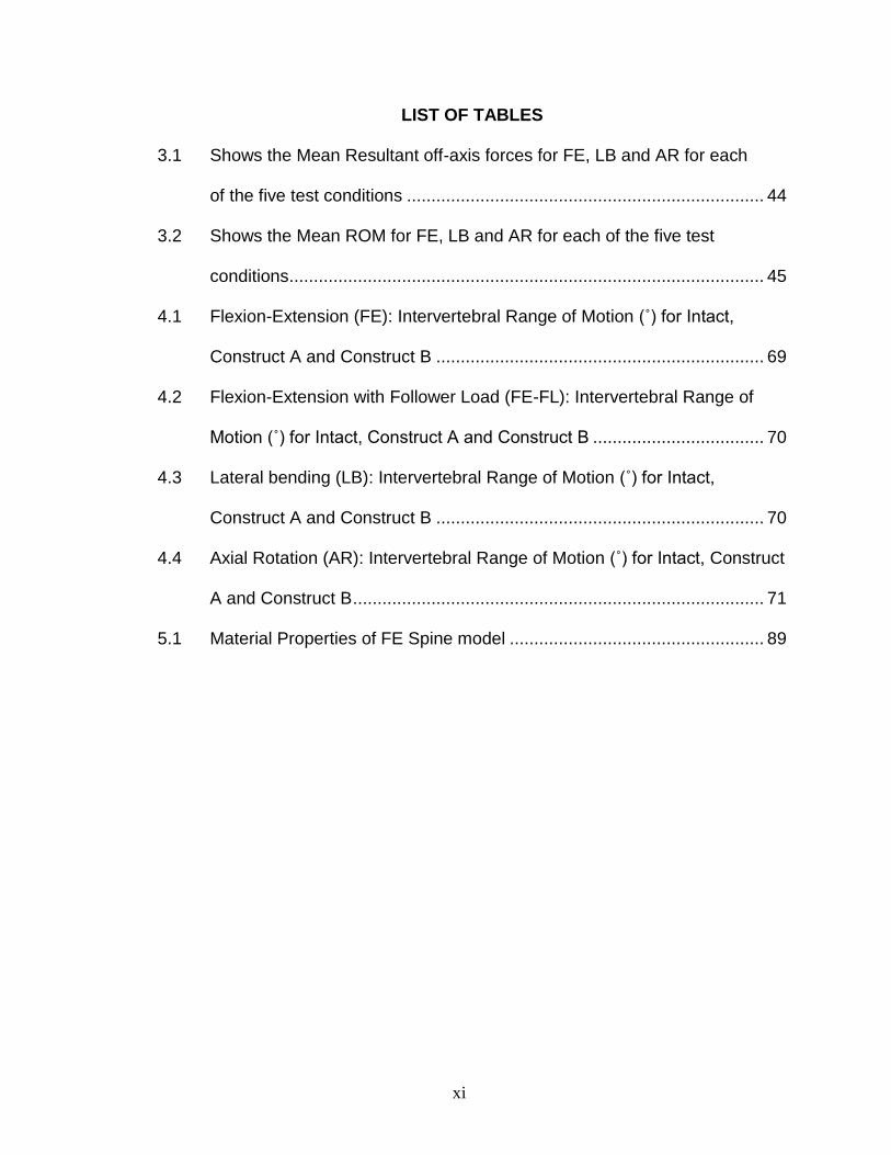
LIST OF TABLES

3.1 Shows the Mean Resultant off-axis forces for FE, LB and AR for each

of the five test conditions ......................................................................... 44

3.2 Shows the Mean ROM for FE, LB and AR for each of the five test

conditions ................................................................................................. 45

4.1 Flexion-Extension (FE): Intervertebral Range of Motion (˚) for Intact,

Construct A and Construct B ................................................................... 69

4.2 Flexion-Extension with Follower Load (FE-FL): Intervertebral Range of

Motion (˚) for Intact, Construct A and Construct B ................................... 70

4.3 Lateral bending (LB): Intervertebral Range of Motion (˚) for Intact,

Construct A and Construct B ................................................................... 70

4.4 Axial Rotation (AR): Intervertebral Range of Motion (˚) for Intact, Construct

A and Construct B .................................................................................... 71

5.1 Material Properties of FE Spine model .................................................... 89

xii

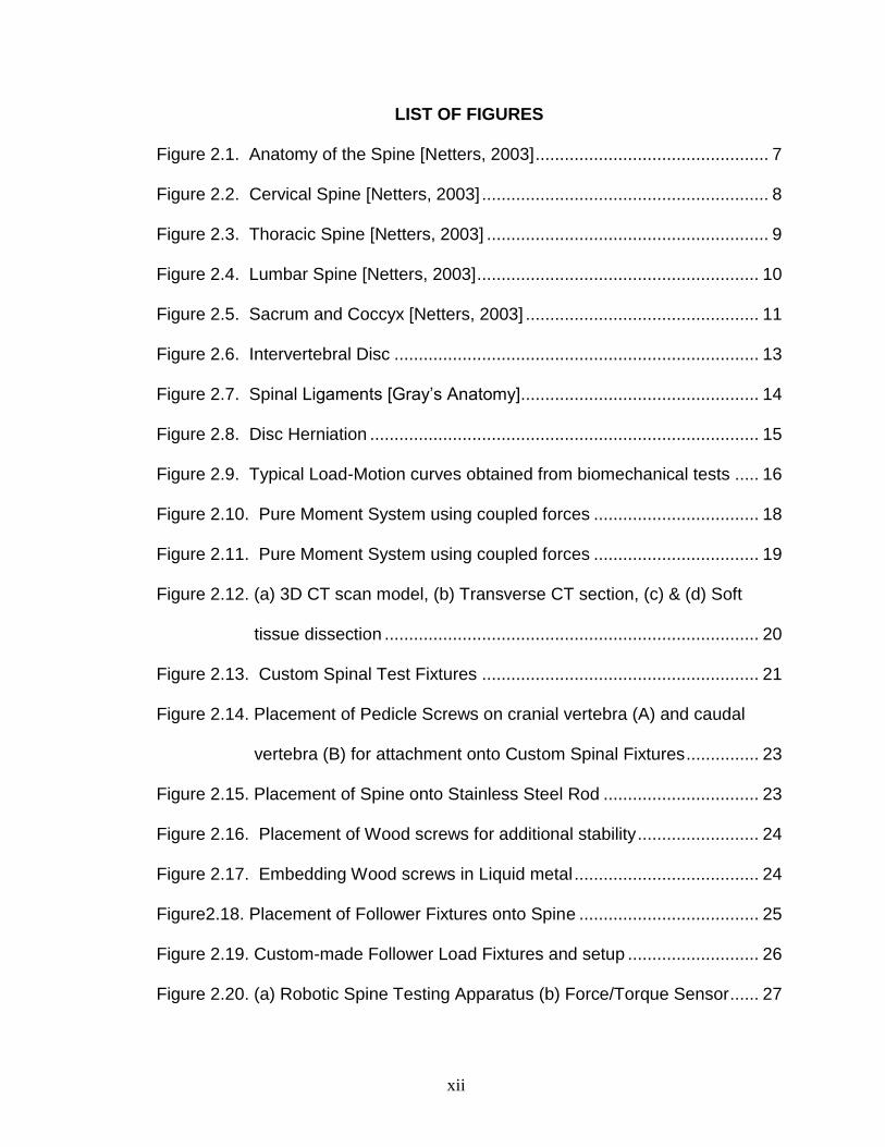
LIST OF FIGURES

Figure 2.1. Anatomy of the Spine [Netters, 2003] ................................................ 7

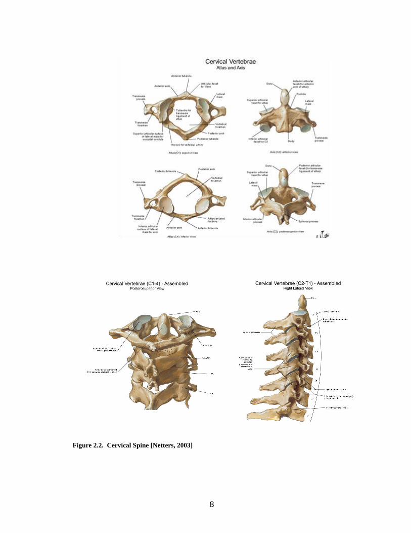
Figure 2.2. Cervical Spine [Netters, 2003] ........................................................... 8

Figure 2.3. Thoracic Spine [Netters, 2003] .......................................................... 9

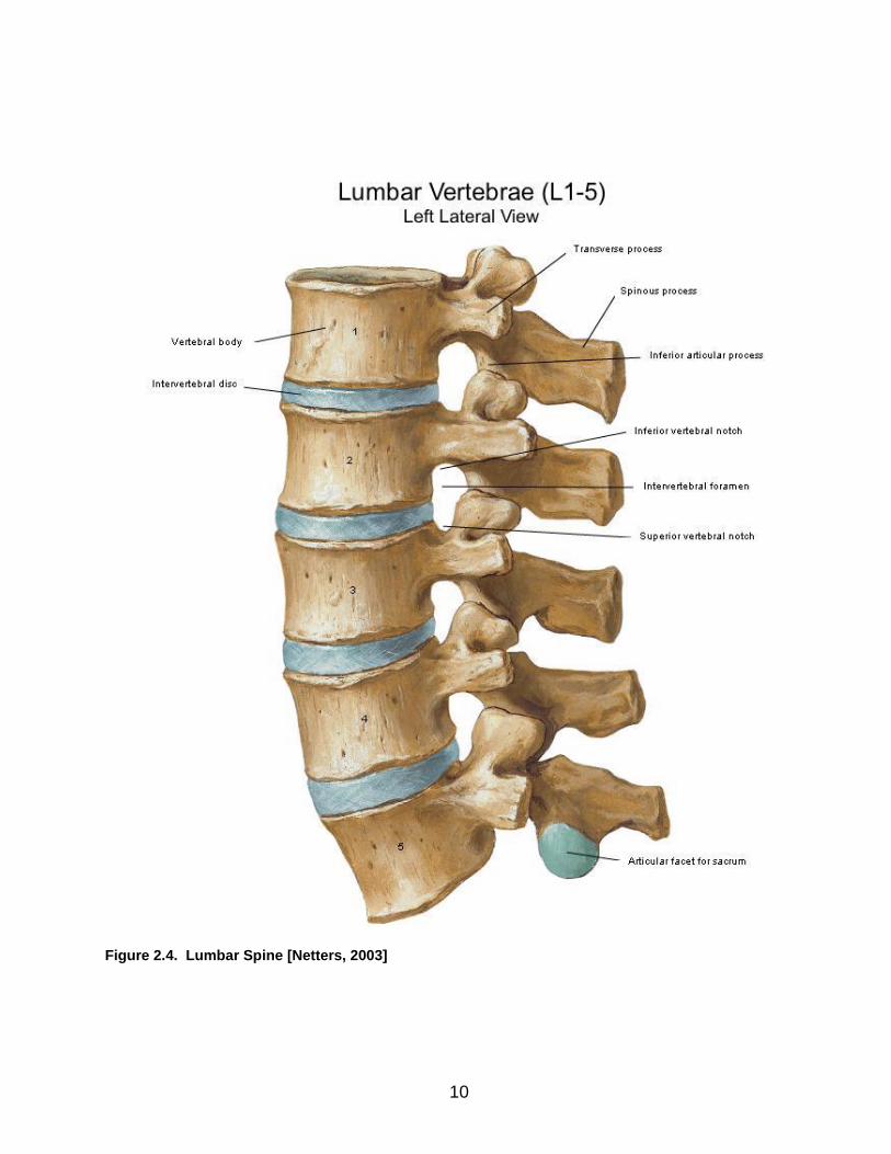
Figure 2.4. Lumbar Spine [Netters, 2003] .......................................................... 10

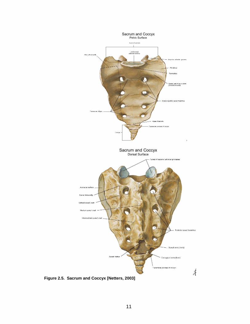
Figure 2.5. Sacrum and Coccyx [Netters, 2003] ................................................ 11

Figure 2.6. Intervertebral Disc ........................................................................... 13

Figure 2.7. Spinal Ligaments [Gray’s Anatomy]................................................. 14

Figure 2.8. Disc Herniation ................................................................................ 15

Figure 2.9. Typical Load-Motion curves obtained from biomechanical tests ..... 16

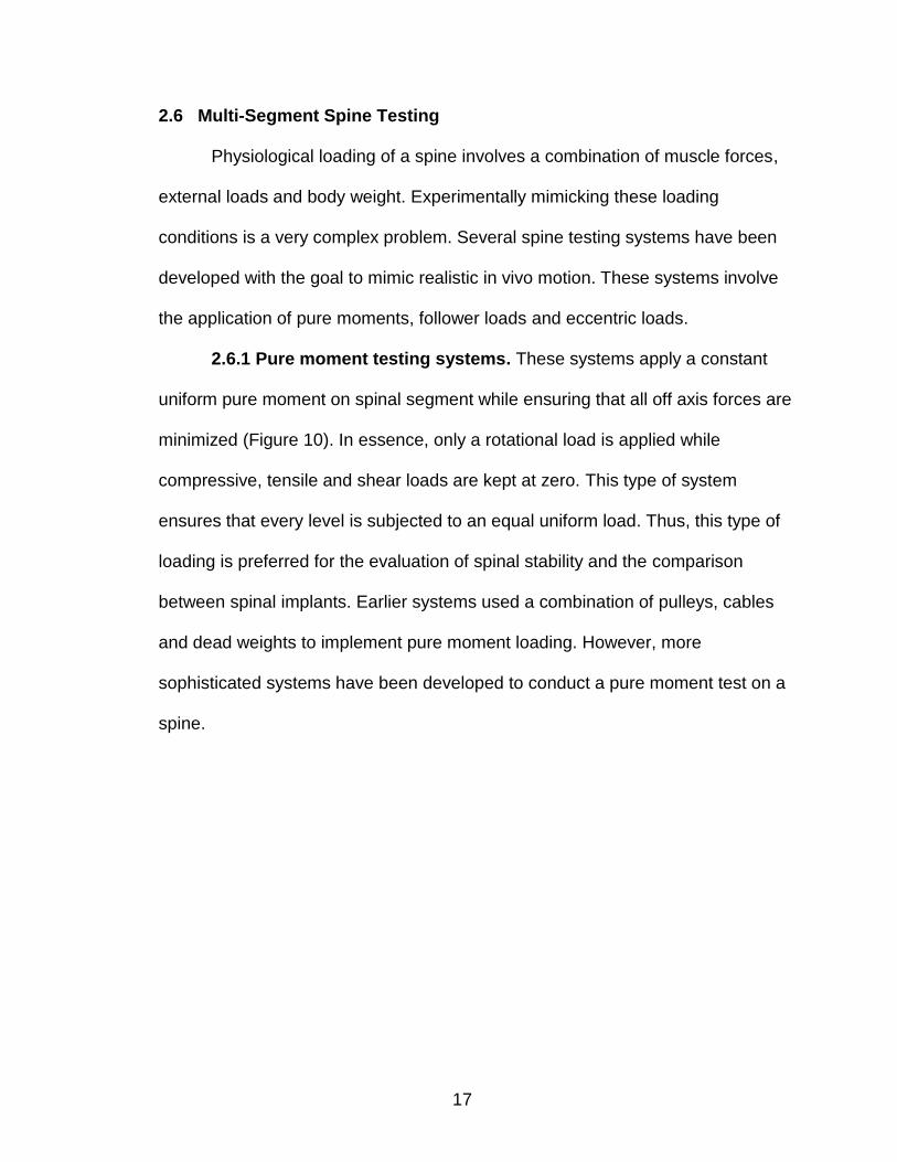
Figure 2.10. Pure Moment System using coupled forces .................................. 18

Figure 2.11. Pure Moment System using coupled forces .................................. 19

Figure 2.12. (a) 3D CT scan model, (b) Transverse CT section, (c) & (d) Soft

tissue dissection ............................................................................. 20

Figure 2.13. Custom Spinal Test Fixtures ......................................................... 21

Figure 2.14. Placement of Pedicle Screws on cranial vertebra (A) and caudal

vertebra (B) for attachment onto Custom Spinal Fixtures ............... 23

Figure 2.15. Placement of Spine onto Stainless Steel Rod ................................ 23

Figure 2.16. Placement of Wood screws for additional stability ......................... 24

Figure 2.17. Embedding Wood screws in Liquid metal ...................................... 24

Figure2.18. Placement of Follower Fixtures onto Spine ..................................... 25

Figure 2.19. Custom-made Follower Load Fixtures and setup ........................... 26

Figure 2.20. (a) Robotic Spine Testing Apparatus (b) Force/Torque Sensor ...... 27

xiii

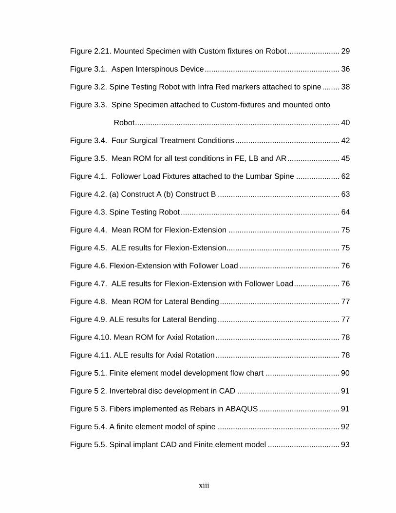
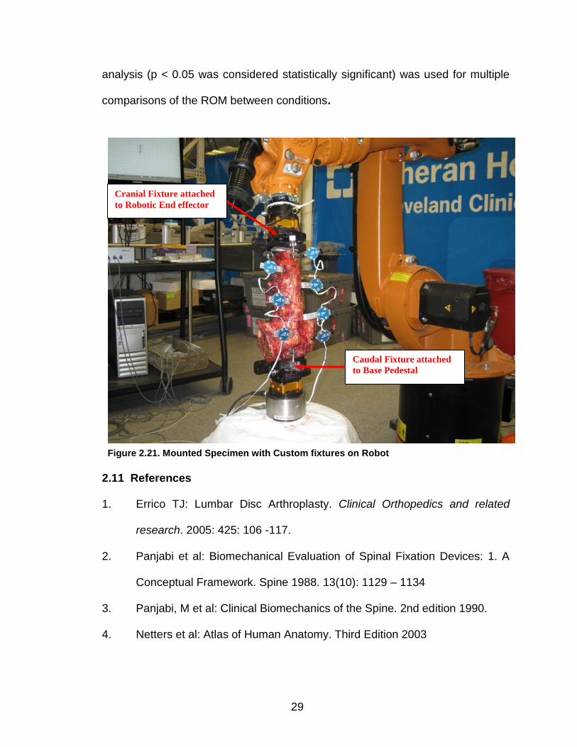
Figure 2.21. Mounted Specimen with Custom fixtures on Robot ........................ 29

Figure 3.1. Aspen Interspinous Device .............................................................. 36

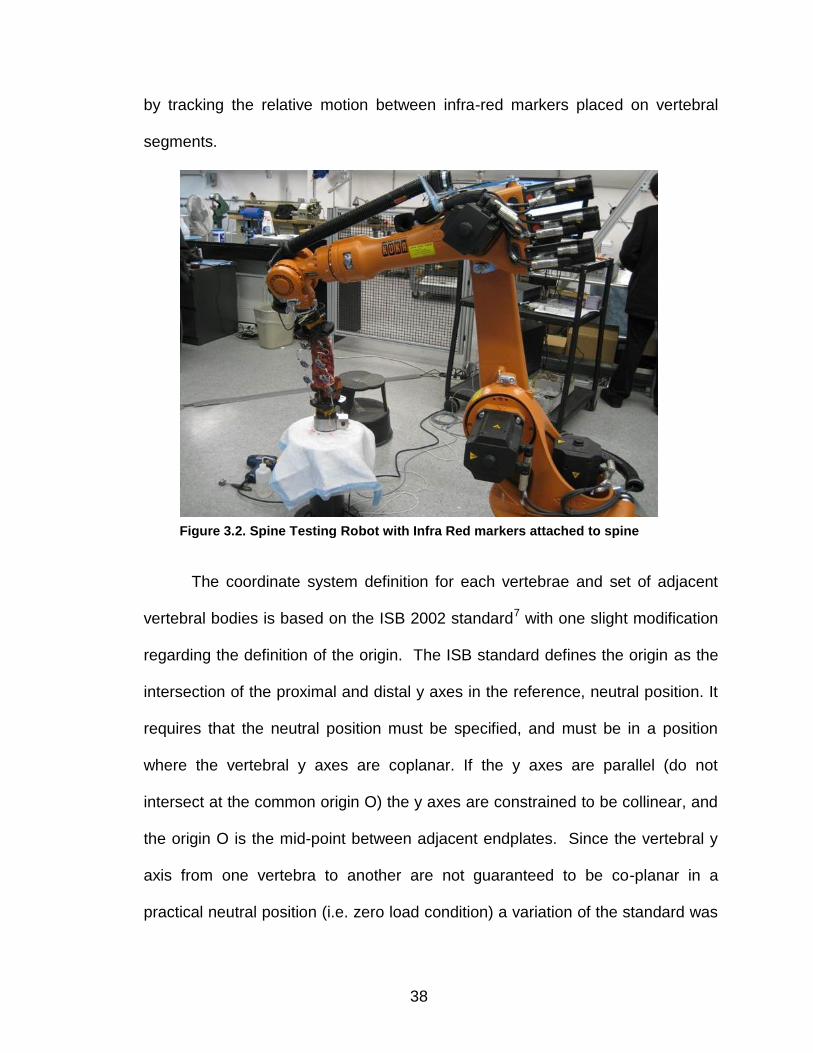
Figure 3.2. Spine Testing Robot with Infra Red markers attached to spine ........ 38

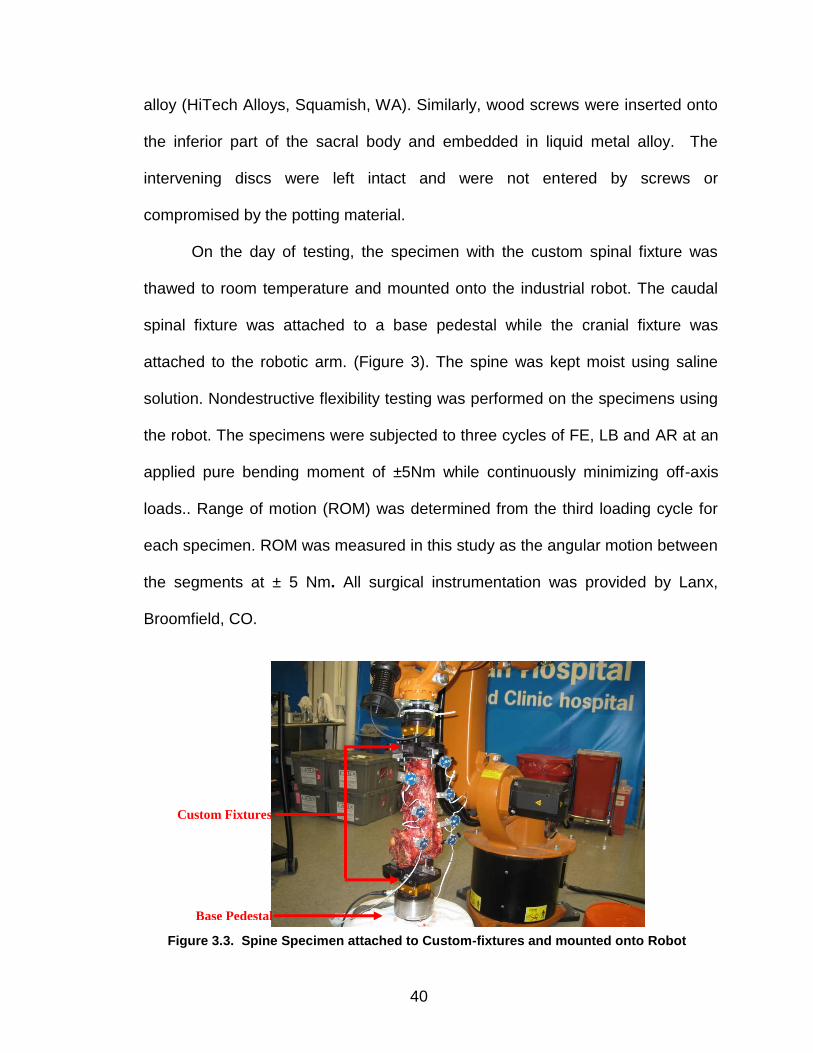
Figure 3.3. Spine Specimen attached to Custom-fixtures and mounted onto

Robot .............................................................................................. 40

Figure 3.4. Four Surgical Treatment Conditions ................................................ 42

Figure 3.5. Mean ROM for all test conditions in FE, LB and AR ........................ 45

Figure 4.1. Follower Load Fixtures attached to the Lumbar Spine .................... 62

Figure 4.2. (a) Construct A (b) Construct B ........................................................ 63

Figure 4.3. Spine Testing Robot ......................................................................... 64

Figure 4.4. Mean ROM for Flexion-Extension ................................................... 75

Figure 4.5. ALE results for Flexion-Extension.................................................... 75

Figure 4.6. Flexion-Extension with Follower Load .............................................. 76

Figure 4.7. ALE results for Flexion-Extension with Follower Load ..................... 76

Figure 4.8. Mean ROM for Lateral Bending ....................................................... 77

Figure 4.9. ALE results for Lateral Bending ........................................................ 77

Figure 4.10. Mean ROM for Axial Rotation ......................................................... 78

Figure 4.11. ALE results for Axial Rotation ......................................................... 78

Figure 5.1. Finite element model development flow chart .................................. 90

Figure 5 2. Invertebral disc development in CAD ............................................... 91

Figure 5 3. Fibers implemented as Rebars in ABAQUS ..................................... 91

Figure 5.4. A finite element model of spine ........................................................ 92

Figure 5.5. Spinal implant CAD and Finite element model ................................. 93

xiv

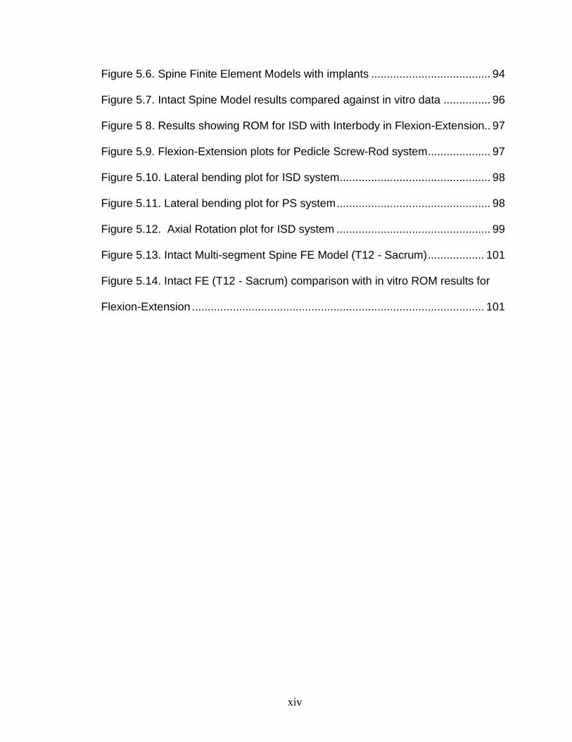
Figure 5.6. Spine Finite Element Models with implants ...................................... 94

Figure 5.7. Intact Spine Model results compared against in vitro data ............... 96

Figure 5 8. Results showing ROM for ISD with Interbody in Flexion-Extension.. 97

Figure 5.9. Flexion-Extension plots for Pedicle Screw-Rod system .................... 97

Figure 5.10. Lateral bending plot for ISD system ................................................ 98

Figure 5.11. Lateral bending plot for PS system ................................................. 98

Figure 5.12. Axial Rotation plot for ISD system ................................................. 99

Figure 5.13. Intact Multi-segment Spine FE Model (T12 - Sacrum) .................. 101

Figure 5.14. Intact FE (T12 - Sacrum) comparison with in vitro ROM results for

Flexion-Extension ............................................................................................. 101

xv

CHAPTER OVERVIEW

A brief overview regarding spine research and the overall research

objectives of the dissertation are stated in the introduction. In chapter 2, an

introduction to the basic anatomy of the spine is highlighted. It also contains a

detailed explanation of the methodology used in conducting a biomechanical test

on spine. It includes description of the basic biomechanical parameters involved

as well as the different testing systems currently available and in use. In chapters

3 and 4, the biomechanical testing of a novel interspinous device and the

adjacent level effects of hybrid dynamic stabilization are described in detail and

the results and conclusions are presented. Chapter 5 describes the development

of a finite element spine model and its validation using test data from in vitro

biomechanical testing of spine.

1

CHAPTER I

INTRODUCTION

Low back pain is one of the most common spine disorders. According to

the Congress for Neurological Surgeons (CNS), 65 million people in the US

annually suffer from low back pain. Treatment costs incurred for back pain

exceed 50 billion dollars per year in the United States alone.1 Studies have also

shown that by age 55, about 85 percent of the population exhibits evidence of

intervertebral disc degeneration which is an initiator of low back pain. Treatment

of back pain upon diagnosis usually involves either a conservative treatment

approach (medications, weight-watch, heat treatment, physical therapy etc.)

and/or surgery (discectomy for decompression of neural elements, fusion with

bone graft and instrumentation for mechanical stabilization).

Spinal fusion is considered the gold standard for the surgical treatment of

intervertebral disc degeneration which causes clinical instability in the spine.

Currently, there are several spinal fusion devices available for use in surgery.

Rapid advancement in basic science research, material science and

manufacturing technologies has led to an increase in novel fusion devices being

developed and made available for the physicians. There is also a push for the

2

development of minimally invasive devices which have the appeal of requiring

smaller incisions, allow for less blood loss and shorter hospital stay. There is also

an increase in the development of motion preserving devices due to the

prevalence of accelerated degeneration of adjacent levels following fusion.

With the current influx of new devices into the medical market, it is

paramount to effectively and systematically evaluate the biomechanical

performance of these new devices and their ability to stabilize the spine.

Biomechanical evaluation of spinal devices has been conducted using three main

standard tests – Failure, Fatigue and Stability. The first two tests are destructive

in nature while the third test is non-destructive in nature. Failure test is used to

assess the device’s ability withstand excessive loading while fatigue test is used

to assess the device’s longevity of use. The stability test involves multi-directional

testing to assess the device’s ability to stabilize the spine. Past studies have

recommended the use of pure moment loading condition in stability tests for the

evaluation of devices.2 Pure bending moment when applied properly causes a

uniform constant load throughout the entire length of the spinal segment making

for more accurate comparison between devices. Several spine testing apparatus

(cable-pulley systems, biaxial and multi-axial spine systems) have been

developed in the past to conduct biomechanical tests on spines under pure

moment loading conditions. Robotic spine testing is a more recent system

currently being used in conducting biomechanical tests. It utilizes a multi-axis

robotic system which provides a flexible testing environment. The robotic system

enables easy changes to be made to the boundary and loading conditions. It also

3

enables unconstrained motion of the spine during testing thereby mimicking in

vivo spinal motion.

The current study is aimed at the development of a methodology for

conducting biomechanical testing of the spine using a robotic system and using

the data from the test to validate a finite element model of a spine. The robotic

system was used to evaluate the performance of two spinal implants - an

interspinous device and a dynamic stabilizer. A finite element model of the spine

was then developed and validated using the data from the biomechanical testing.

4

CHAPTER II

BIOMECHANICAL TESTING OF SPINE

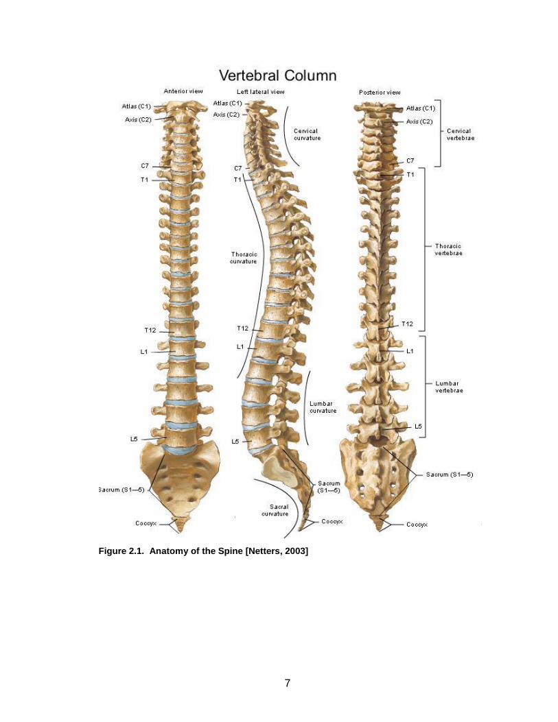
2.1 Spinal Anatomy

The human spine (vertebral column) is composed of vertebrae (singular –

vertebra) and intervertebral discs. The vertebrae articulate on each other and are

supported structurally by spinal ligaments. The main function of the human spine

is to protect the neural elements (spinal cord and nerves). Other functions are to

support the body weight, provide posture and locomotion. The vertebra mainly

consists of the vertebral body (anterior part of the vertebra), vertebral arch

(posterior part of the vertebra, consists of two pedicles and lamina), two

transverse process, one spinous process and four articulating facets (two

superior and two inferior). A functional spinal unit (FSU) is referred to as the

smallest segment of the spine that exhibits similar biomechanical characteristics

as a whole spine.3 It basically consists of two adjacent vertebrae, the

intervertebral disc and spinal ligaments. Biomechanical testing on the spine

typically involves the use of either single FSU or multisegmental spinal units.

5

The human spine is divided into 5 regions: cervical, thoracic, lumbar,

sacral, and coccygeal (Figure 1). The cervical spine is the most superior region

and located close to the head (cranial) while coccygeal is the most inferior region

that is located closer to the feet (caudal). The anatomical differences between

each regions result in differences in their biomechanical characteristics. The

orientation of the articulating facet joints, vertebral body size between the

regions, all play a considerable role in contributing towards the variation in

kinematics of each region.

Cervical Spine – The cervical spine is located between the head

(cranium) and the thoracic vertebrae. They are the smallest of the

spinal vertebrae. There are a total of seven cervical vertebrae

anatomically labeled C1 through to C7. The two superior vertebrae,

C1 and C2 are also known as Atlas and Axis. They are

anatomically different from the other cervical vertebrae. Atlas has

no vertebral body or spinous process while the Axis has a

prominent protrusion called the Odontoid process (dens) that

projects superiorly from the vertebral body. Figure 2 shows an

illustration of the cervical spine. In the sagittal plane, the cervical

spine has a convex-shaped curve anteriorly (Lordosis).

Thoracic Spine – The thoracic spine is located in the upper back

between the cervical vertebrae and the lumbar vertebrae. There are

a total of twelve thoracic vertebrae anatomically labeled T1 to T12.

These vertebrae also provide attachments for the ribs and thus

6

contain costal facets for articulation with the ribs. An identifying

anatomic feature is the spinous process typically projects

downwards. In the sagittal plane, the thoracic spine has a concave

curvature (Kyphosis) anteriorly. Figure 3 shows an illustration of the

thoracic spine.

Lumbar Spine – The lumbar spine is located in the lower back

between the thoracic spine and sacrum. There are five lumbar

vertebrae, anatomically labeled L1 to L5. They have larger vertebral

bodies than thoracic or cervical spine. In the sagittal plane, the

Lumbar spine has a convex curvature (Lordosis) anteriorly. Figure

4 shows an illustration of the lumbar spine.

Sacrum and Coccyx – The sacrum is located caudal to the lumbar

spine. It consists of about five fused vertebrae. The coccyx is

located caudal to the sacrum and is made up of four fused

vertebrae. Figure 5 shows an illustration of the Sacrum and

Coccyx.

7

Figure 2.1. Anatomy of the Spine [Netters, 2003]

8

Figure 2.2. Cervical Spine [Netters, 2003]

9

Figure 2.3. Thoracic Spine [Netters, 2003]

10

Figure 2.4. Lumbar Spine [Netters, 2003]

11

Figure 2.5. Sacrum and Coccyx [Netters, 2003]

12

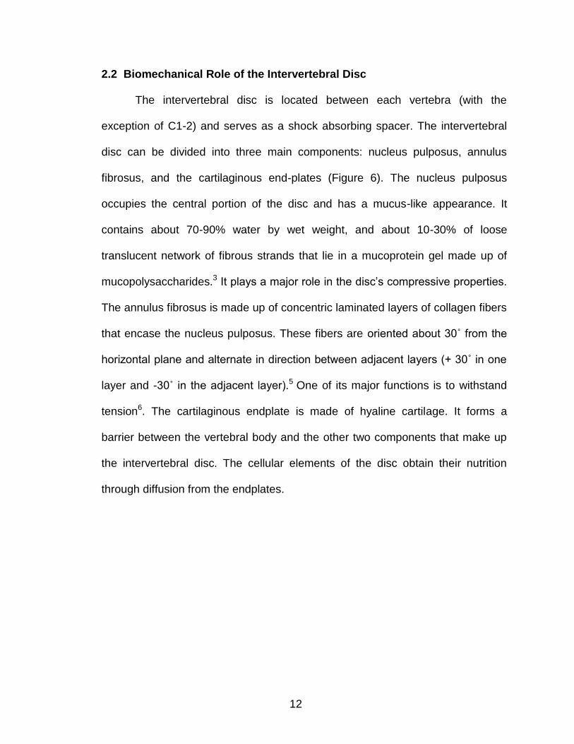
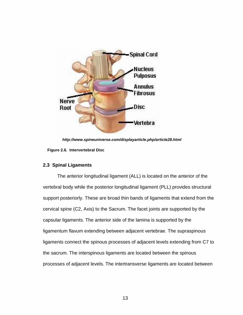
2.2 Biomechanical Role of the Intervertebral Disc

The intervertebral disc is located between each vertebra (with the

exception of C1-2) and serves as a shock absorbing spacer. The intervertebral

disc can be divided into three main components: nucleus pulposus, annulus

fibrosus, and the cartilaginous end-plates (Figure 6). The nucleus pulposus

occupies the central portion of the disc and has a mucus-like appearance. It

contains about 70-90% water by wet weight, and about 10-30% of loose

translucent network of fibrous strands that lie in a mucoprotein gel made up of

mucopolysaccharides.3 It plays a major role in the disc’s compressive properties.

The annulus fibrosus is made up of concentric laminated layers of collagen fibers

that encase the nucleus pulposus. These fibers are oriented about 30˚ from the

horizontal plane and alternate in direction between adjacent layers (+ 30˚ in one

layer and -30˚ in the adjacent layer).5 One of its major functions is to withstand

tension6. The cartilaginous endplate is made of hyaline cartilage. It forms a

barrier between the vertebral body and the other two components that make up

the intervertebral disc. The cellular elements of the disc obtain their nutrition

through diffusion from the endplates.

13

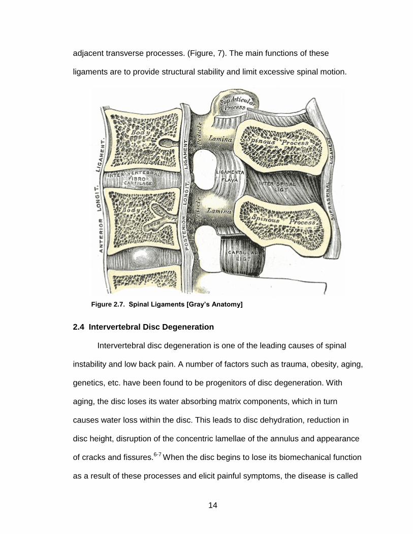
2.3 Spinal Ligaments

The anterior longitudinal ligament (ALL) is located on the anterior of the

vertebral body while the posterior longitudinal ligament (PLL) provides structural

support posteriorly. These are broad thin bands of ligaments that extend from the

cervical spine (C2, Axis) to the Sacrum. The facet joints are supported by the

capsular ligaments. The anterior side of the lamina is supported by the

ligamentum flavum extending between adjacent vertebrae. The supraspinous

ligaments connect the spinous processes of adjacent levels extending from C7 to

the sacrum. The interspinous ligaments are located between the spinous

processes of adjacent levels. The intertransverse ligaments are located between

http://www.spineuniverse.com/displayarticle.php/article28.html

Figure 2.6. Intervertebral Disc

14

adjacent transverse processes. (Figure, 7). The main functions of these

ligaments are to provide structural stability and limit excessive spinal motion.

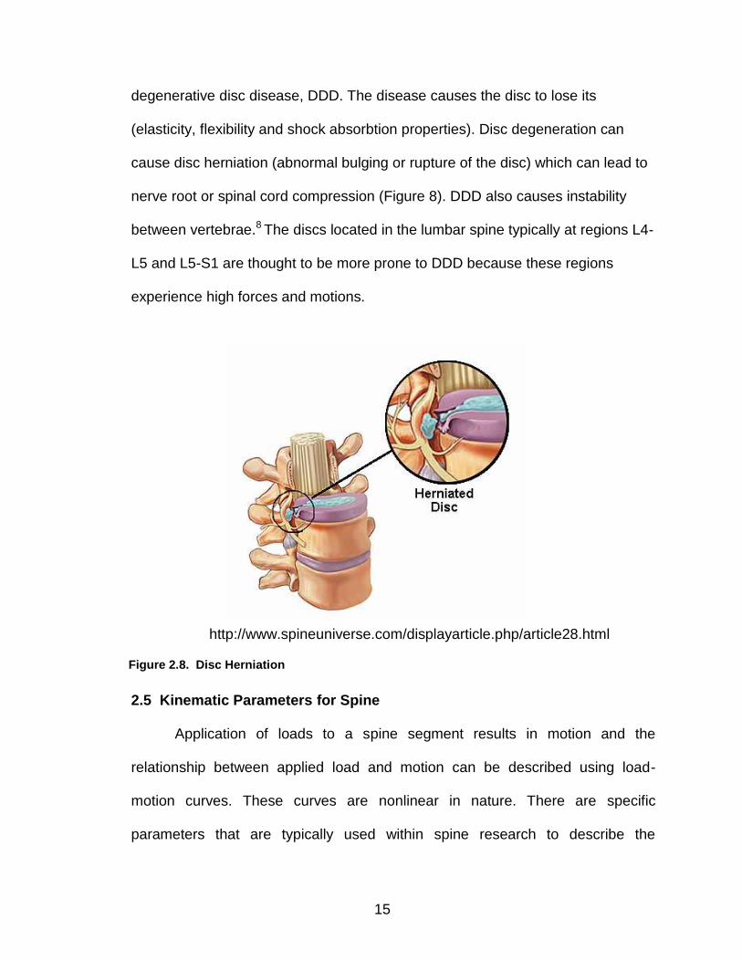
2.4 Intervertebral Disc Degeneration

Intervertebral disc degeneration is one of the leading causes of spinal

instability and low back pain. A number of factors such as trauma, obesity, aging,

genetics, etc. have been found to be progenitors of disc degeneration. With

aging, the disc loses its water absorbing matrix components, which in turn

causes water loss within the disc. This leads to disc dehydration, reduction in

disc height, disruption of the concentric lamellae of the annulus and appearance

of cracks and fissures.6-7 When the disc begins to lose its biomechanical function

as a result of these processes and elicit painful symptoms, the disease is called

Figure 2.7. Spinal Ligaments [Gray’s Anatomy]

15

degenerative disc disease, DDD. The disease causes the disc to lose its

(elasticity, flexibility and shock absorbtion properties). Disc degeneration can

cause disc herniation (abnormal bulging or rupture of the disc) which can lead to

nerve root or spinal cord compression (Figure 8). DDD also causes instability

between vertebrae.8 The discs located in the lumbar spine typically at regions L4-

L5 and L5-S1 are thought to be more prone to DDD because these regions

experience high forces and motions.

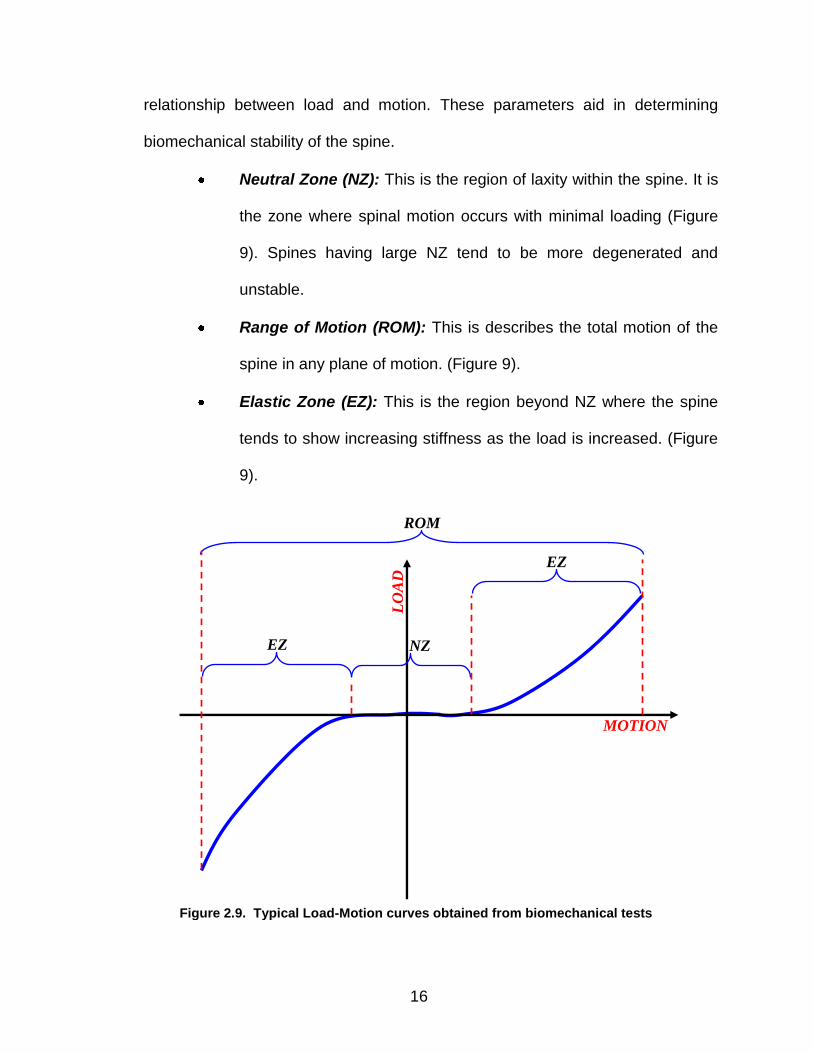
2.5 Kinematic Parameters for Spine

Application of loads to a spine segment results in motion and the

relationship between applied load and motion can be described using load-

motion curves. These curves are nonlinear in nature. There are specific

parameters that are typically used within spine research to describe the

http://www.spineuniverse.com/displayarticle.php/article28.html

Figure 2.8. Disc Herniation

16

relationship between load and motion. These parameters aid in determining

biomechanical stability of the spine.

Neutral Zone (NZ): This is the region of laxity within the spine. It is

the zone where spinal motion occurs with minimal loading (Figure

9). Spines having large NZ tend to be more degenerated and

unstable.

Range of Motion (ROM): This is describes the total motion of the

spine in any plane of motion. (Figure 9).

Elastic Zone (EZ): This is the region beyond NZ where the spine

tends to show increasing stiffness as the load is increased. (Figure

9).

MOTION

LO

AD

EZ

EZ

ROM

NZ

Figure 2.9. Typical Load-Motion curves obtained from biomechanical tests

17

2.6 Multi-Segment Spine Testing

Physiological loading of a spine involves a combination of muscle forces,

external loads and body weight. Experimentally mimicking these loading

conditions is a very complex problem. Several spine testing systems have been

developed with the goal to mimic realistic in vivo motion. These systems involve

the application of pure moments, follower loads and eccentric loads.

2.6.1 Pure moment testing systems. These systems apply a constant

uniform pure moment on spinal segment while ensuring that all off axis forces are

minimized (Figure 10). In essence, only a rotational load is applied while

compressive, tensile and shear loads are kept at zero. This type of system

ensures that every level is subjected to an equal uniform load. Thus, this type of

loading is preferred for the evaluation of spinal stability and the comparison

between spinal implants. Earlier systems used a combination of pulleys, cables

and dead weights to implement pure moment loading. However, more

sophisticated systems have been developed to conduct a pure moment test on a

spine.

18

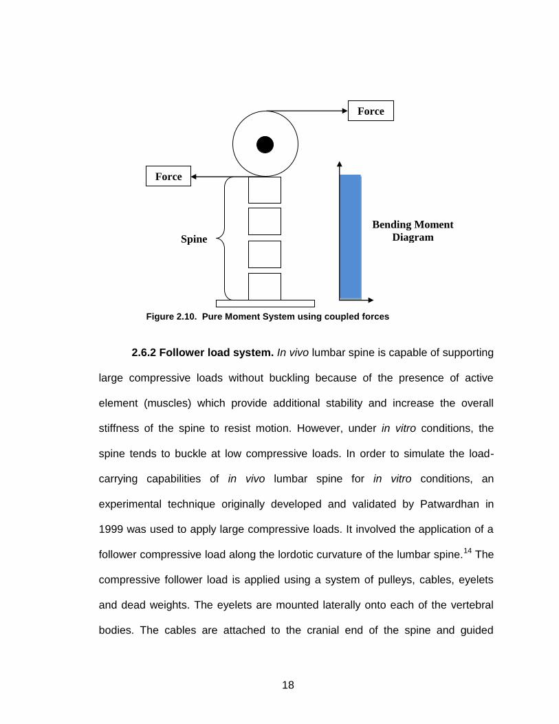
2.6.2 Follower load system. In vivo lumbar spine is capable of supporting

large compressive loads without buckling because of the presence of active

element (muscles) which provide additional stability and increase the overall

stiffness of the spine to resist motion. However, under in vitro conditions, the

spine tends to buckle at low compressive loads. In order to simulate the load-

carrying capabilities of in vivo lumbar spine for in vitro conditions, an

experimental technique originally developed and validated by Patwardhan in

1999 was used to apply large compressive loads. It involved the application of a

follower compressive load along the lordotic curvature of the lumbar spine.14 The

compressive follower load is applied using a system of pulleys, cables, eyelets

and dead weights. The eyelets are mounted laterally onto each of the vertebral

bodies. The cables are attached to the cranial end of the spine and guided

Force

Force

Spine

Bending Moment

Diagram

Figure 2.10. Pure Moment System using coupled forces

19

through each of the eyelets. The positions of the eyelets are adjusted to

approximate the center of the vertebral bodies and enable the load path to follow

the curvature of the lumbar spine.

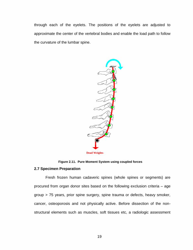
2.7 Specimen Preparation

Fresh frozen human cadaveric spines (whole spines or segments) are

procured from organ donor sites based on the following exclusion criteria – age

group > 75 years, prior spine surgery, spine trauma or defects, heavy smoker,

cancer, osteoporosis and not physically active. Before dissection of the non-

structural elements such as muscles, soft tissues etc, a radiologic assessment

Dead Weights

Figure 2.11. Pure Moment System using coupled forces

20

using Computed Tomography (CT) and a visual inspection were made to exclude

any bony defects such as fractures and soft tissue abnormalities.

The specimens were then dissected to remove all non-ligamentous soft

tissue (non-structural) while preserving the vertebral bodies, discs, facet joint

capsules and the following ligamentous soft tissues (structural) – anterior

longitudinal ligament (ALL), posterior longitudinal ligament (PLL), the

interspinous and the supraspinous ligament. (Figure 12).

2.8 Custom Spinal Test Fixtures

Custom test fixtures (Figure 13) were designed to secure the spine

specimen for biomechanical testing based on anthropometric data.9-13 The

Figure 2.12. (a) 3D CT scan model, (b) Transverse CT section, (c) & (d) Soft tissue dissection

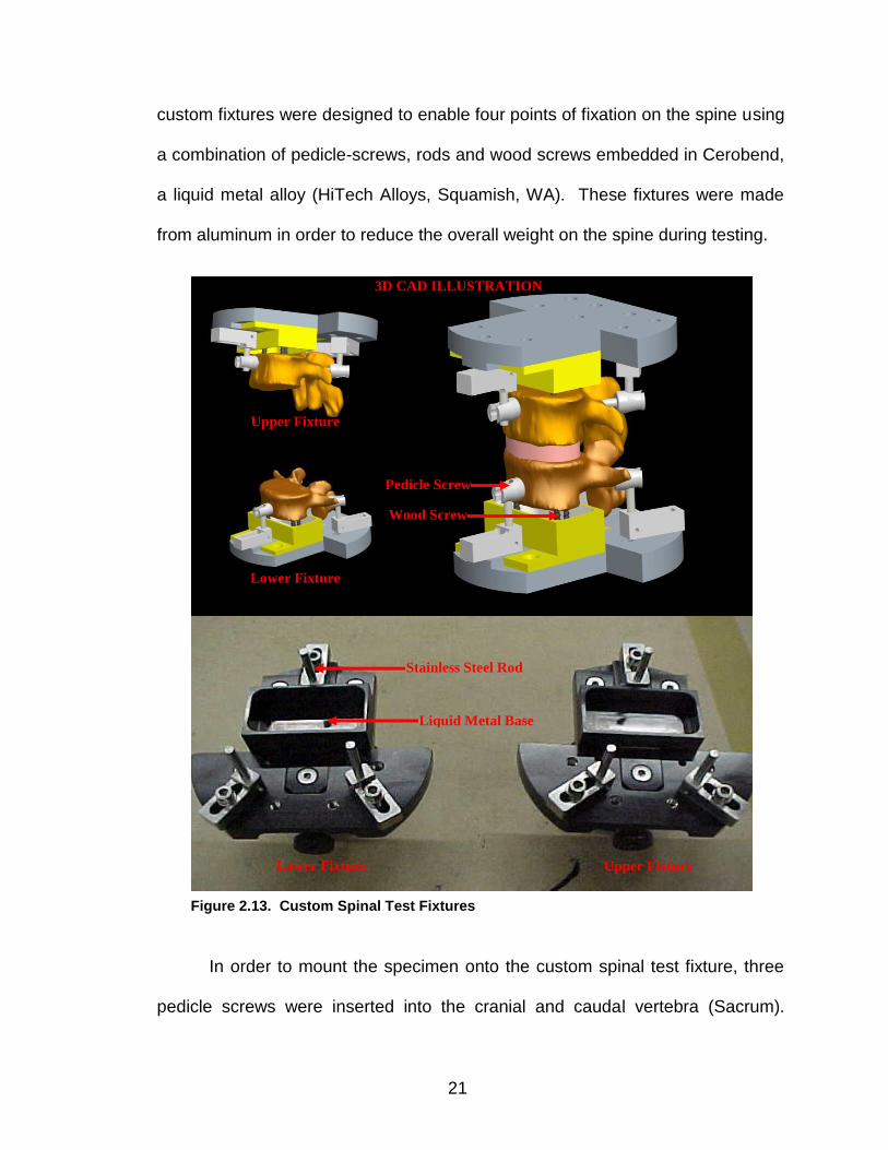
21

custom fixtures were designed to enable four points of fixation on the spine using

a combination of pedicle-screws, rods and wood screws embedded in Cerobend,

a liquid metal alloy (HiTech Alloys, Squamish, WA). These fixtures were made

from aluminum in order to reduce the overall weight on the spine during testing.

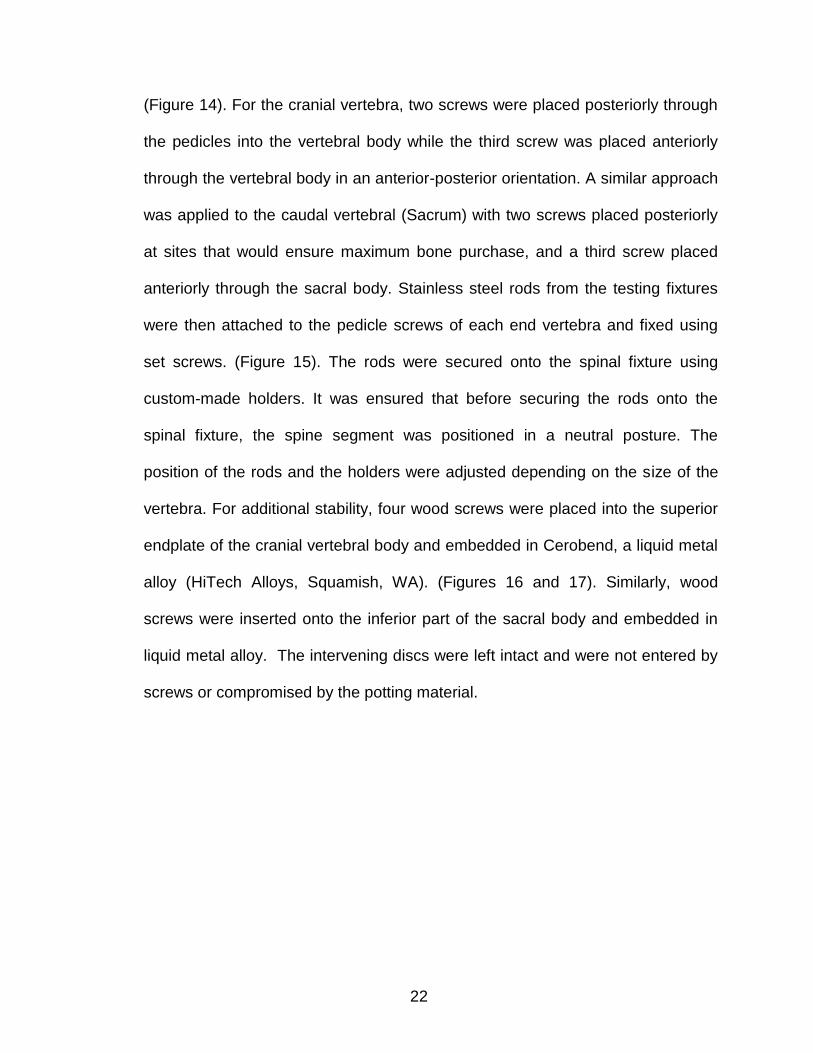
In order to mount the specimen onto the custom spinal test fixture, three

pedicle screws were inserted into the cranial and caudal vertebra (Sacrum).

Lower Fixture Upper Fixture

Lower Fixture

Upper Fixture

Pedicle Screw

Liquid Metal Base

Wood Screw

3D CAD ILLUSTRATION

Stainless Steel Rod

Figure 2.13. Custom Spinal Test Fixtures

22

(Figure 14). For the cranial vertebra, two screws were placed posteriorly through

the pedicles into the vertebral body while the third screw was placed anteriorly

through the vertebral body in an anterior-posterior orientation. A similar approach

was applied to the caudal vertebral (Sacrum) with two screws placed posteriorly

at sites that would ensure maximum bone purchase, and a third screw placed

anteriorly through the sacral body. Stainless steel rods from the testing fixtures

were then attached to the pedicle screws of each end vertebra and fixed using

set screws. (Figure 15). The rods were secured onto the spinal fixture using

custom-made holders. It was ensured that before securing the rods onto the

spinal fixture, the spine segment was positioned in a neutral posture. The

position of the rods and the holders were adjusted depending on the size of the

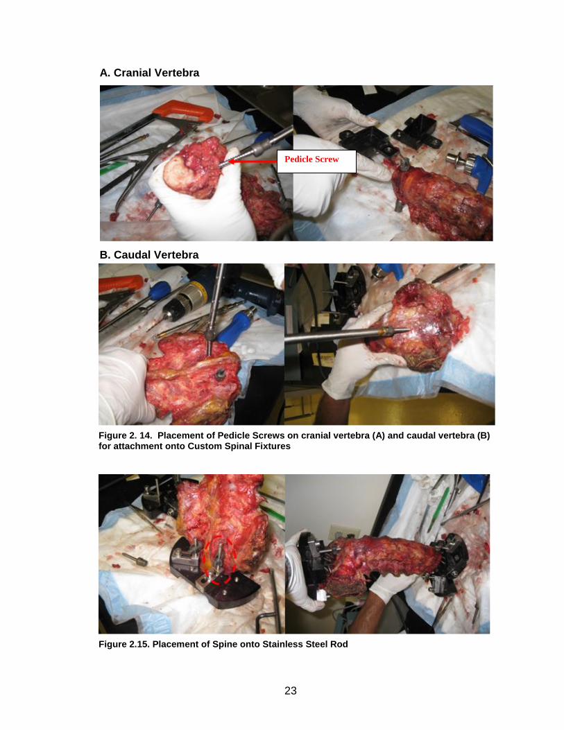
vertebra. For additional stability, four wood screws were placed into the superior

endplate of the cranial vertebral body and embedded in Cerobend, a liquid metal

alloy (HiTech Alloys, Squamish, WA). (Figures 16 and 17). Similarly, wood

screws were inserted onto the inferior part of the sacral body and embedded in

liquid metal alloy. The intervening discs were left intact and were not entered by

screws or compromised by the potting material.

23

A. Cranial Vertebra

B. Caudal Vertebra

Pedicle Screw

Figure 2. 14. Placement of Pedicle Screws on cranial vertebra (A) and caudal vertebra (B) for attachment onto Custom Spinal Fixtures

Figure 2.15. Placement of Spine onto Stainless Steel Rod

24

Figure 2.17. Embedding Wood screws in Liquid metal

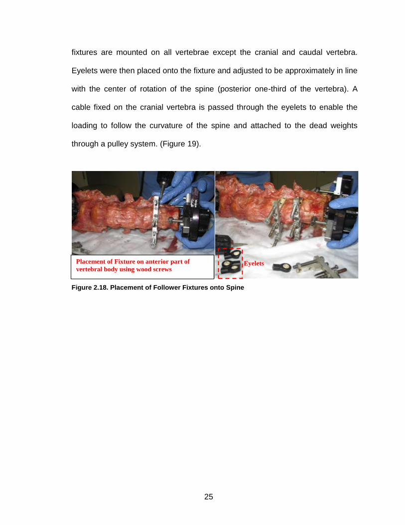
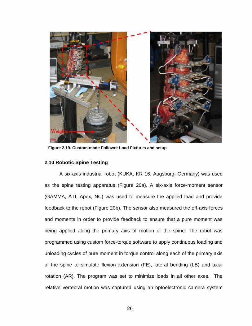
2.9 Follower Load Fixtures

Custom fixtures were designed and developed based on the follower load

model to apply compressive loads during the robotic biomechanical testing. Dead

weights were used to apply the compressive load. The follower load fixtures were

mounted anteriorly onto the vertebrae using wood screws. (Figure 18) The

Liquid Metal

Figure 2.16. Placement of Wood screws for additional stability

25

fixtures are mounted on all vertebrae except the cranial and caudal vertebra.

Eyelets were then placed onto the fixture and adjusted to be approximately in line

with the center of rotation of the spine (posterior one-third of the vertebra). A

cable fixed on the cranial vertebra is passed through the eyelets to enable the

loading to follow the curvature of the spine and attached to the dead weights

through a pulley system. (Figure 19).

Figure 2.18. Placement of Follower Fixtures onto Spine

Placement of Fixture on anterior part of

vertebral body using wood screws Eyelets

26

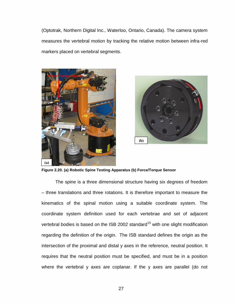
2.10 Robotic Spine Testing

A six-axis industrial robot (KUKA, KR 16, Augsburg, Germany) was used

as the spine testing apparatus (Figure 20a). A six-axis force-moment sensor

(GAMMA, ATI, Apex, NC) was used to measure the applied load and provide

feedback to the robot (Figure 20b). The sensor also measured the off-axis forces

and moments in order to provide feedback to ensure that a pure moment was

being applied along the primary axis of motion of the spine. The robot was

programmed using custom force-torque software to apply continuous loading and

unloading cycles of pure moment in torque control along each of the primary axis

of the spine to simulate flexion-extension (FE), lateral bending (LB) and axial

rotation (AR). The program was set to minimize loads in all other axes. The

relative vertebral motion was captured using an optoelectronic camera system

Eyelets

Mounted

Fixture

Figure 2.19. Custom-made Follower Load Fixtures and setup

27

(Optotrak, Northern Digital Inc., Waterloo, Ontario, Canada). The camera system

measures the vertebral motion by tracking the relative motion between infra-red

markers placed on vertebral segments.

The spine is a three dimensional structure having six degrees of freedom

– three translations and three rotations. It is therefore important to measure the

kinematics of the spinal motion using a suitable coordinate system. The

coordinate system definition used for each vertebrae and set of adjacent

vertebral bodies is based on the ISB 2002 standard15 with one slight modification

regarding the definition of the origin. The ISB standard defines the origin as the

intersection of the proximal and distal y axes in the reference, neutral position. It

requires that the neutral position must be specified, and must be in a position

where the vertebral y axes are coplanar. If the y axes are parallel (do not

(a)

(b)

Force/Torque Sensor

Figure 2.20. (a) Robotic Spine Testing Apparatus (b) Force/Torque Sensor

28

intersect at the common origin O) the y axes are constrained to be collinear, and

the origin O is the mid-point between adjacent endplates. Since the vertebral y

axis from one vertebra to another are not guaranteed to be co-planar in a

practical neutral position (i.e. zero load condition) a variation of the standard was

implemented. The axis intersection point was not used and the mid-point

between adjacent endplates was estimated as the midpoint of the two vertebral

origins. Though these points are not guaranteed to be the same, they are likely

close enough and will allow for multiple vertebral kinematics to be calculated

without having to have two origins per vertebra.

The spine specimen with the custom spinal fixture was mounted onto the

industrial robot by attaching, first, the caudal spinal fixture to a fixed base

pedestal and then the free end, the cranial fixture, is attached to the robotic end

effector. (Figure 21). The spine was kept moist using saline solution.

Nondestructive flexibility testing was performed on the specimens using the robot

to compare various treatments. The specimens are subjected to three cycles of

pure bending moment while continuously minimizing off-axis loads. Range of

motion (ROM) was determined from the third loading cycle for each specimen.

ROM is the total angular rotation between vertebral bodies.

Statistical analysis was performed using Minitab 16 (Minitab Inc., State

College, PA) to compare the differences between treatments. A repeated

measures analysis of variance was used to analyze the ROM between test

conditions with a 95% level of significance. Post-hoc Tukey-Kramer or Bonferroni

29

analysis (p < 0.05 was considered statistically significant) was used for multiple

comparisons of the ROM between conditions.

2.11 References

1. Errico TJ: Lumbar Disc Arthroplasty. Clinical Orthopedics and related

research. 2005: 425: 106 -117.

2. Panjabi et al: Biomechanical Evaluation of Spinal Fixation Devices: 1. A

Conceptual Framework. Spine 1988. 13(10): 1129 – 1134

3. Panjabi, M et al: Clinical Biomechanics of the Spine. 2nd edition 1990.

4. Netters et al: Atlas of Human Anatomy. Third Edition 2003

Cranial Fixture attached

to Robotic End effector

Caudal Fixture attached

to Base Pedestal

Figure 2.21. Mounted Specimen with Custom fixtures on Robot

30

5. Marchand F, Ahmed AM. Investigation of the laminate structure of lumbar

disc anulus fibrosus. Spine (Phila Pa 1976). 1990 May;15(5):402-10.

6. Herkowitz, HN et al: The Spine, Vol. 1. 5th edition. 2006

7. An et. al.: Relevance of In Vitro and In Vivo models for Intervertebral Disc

Degeneration. J Bone and Joint Surgery. 2006:88:88-94.

8. Shedid, D: Lumbar total disc replacement compared with spinal fusion:

treatment choice and evaluation of outcome. Nat Clin Pract Neurol.

2005:1:4-5.

9. Panjabi MM, Oxland TR, Parks EH: Quantitative anatomy of cervical spine

ligaments. Part I. Upper cervical spine. J Spinal

Disord. 1991 Sep;4(3):270-6.

10. Panjabi MM, Oxland TR, Parks EH: Quantitative anatomy of cervical spine

ligaments. Part II. Middle and lower cervical spine.J Spinal

Disord. 1991 Sep;4(3):277-85.

11. Panjabi MM, Takata K, Goel V, Federico D, Oxland T, Duranceau J, Krag

M. Thoracic human vertebrae. Quantitative three-dimensional anatomy.

Spine. 1991 Aug;16(8):888-901.

12. Panjabi MM, Goel V, Oxland T, Takata K, Duranceau J, Krag M, Price M.

Human lumbar vertebrae. Quantitative three-dimensional

anatomy.Spine. 1992 Mar;17(3):299-306.

13. Zhou et. al.: Geometrical dimensions of the lower lumbar vertebrae

analysis of data from digitized CT images. Eur. Spine J. 2000:9:242-248.

31

14. Patwardan et al: A follower load increases the load-carrying capacity of

the lumbar spine in compression. Spine. 1999 May 15;24(10):1003-9.

15. Wu G, Siegler S, Allard P, Kirtley C, Leardini A, Rosenbaum D, Whittle M,

D'Lima DD, Cristofolini L, Witte H, Schmid O, Stokes I. ISB

recommendation on definitions of joint coordinate system of various joints

for the reporting of human joint motion--part I: ankle, hip, and spine.

International Society of Biomechanics.; Standardization and Terminology

Committee of the International Society of Biomechanics. J Biomech. 2002.

35(4):543-8.

32

CHAPTER III

PROPERTIES OF AN INTERSPINOUS FIXATION DEVICE (ISD) IN LUMBAR

FUSION CONSTRUCTS: A BIOMECHANICAL STUDY

(Submitted for publication – The Spine Journal)

3.1 Abstract

3.1.1 Introduction. Segmental fixation improves fusion rates and

promotes mobility after lumbar surgery. Efforts to obtain stability using less

invasive techniques have lead to the advent of new implants and constructs. A

new interspinous fixation device (ISD) has been introduced as a minimally

invasive method of stabilizing two adjacent interspinous (IS) processes while the

fusion occurs. Used to augment an interbody cage in transforaminal interbody

fusion, the ISD is intended to replace the standard pedicle screw instrumentation

used for posterior fixation. The ISD was evaluated using the standard

biomechanical testing methods. The purpose of this study is to compare the

rigidity of these implant systems when supplementing an interbody cage as used

in transforaminal lumbar interbody fusion (TLIF). The overall goal of this study

was to utilize the robotic system to conduct the in vitro tests and assess the

stability of the ISD in relation to the spine.

33

3.1.2 Methods. Seven human cadaver spines (T12 to the sacrum) were

mounted in a custom designed testing apparatus, then mounted for

biomechanical testing using a multiaxial robotic system. A comparison of

segmental stiffness was carried out among four instrumentation constructs: 1)

intact spine control, 2) Interbody cage, alone (IBC), 3) Interbody Cage with

Interspinous Fixation Device (ISD), 4) Interbody Cage, Interspinous Fixation

Device and unilateral pedicle screws (Unilat), 5) Interbody Cage,with bilateral

pedicle screws (Bilat). An industrial robot (KUKA, GmbH, Augsburg, Germany)

applied a pure moment (±5 Nm) in flexion-extension (FE), lateral bending (LB)

and axial rotation (AR) through an anchor to the T12 vertebral body. The relative

vertebral motion was captured using an optoelectronic camera system (Optotrak,

Northern Digital Inc., Waterloo, ON, Canada). The load sensor and the camera

were synchronized. Maximum displacement was measured at each level and

stiffness of the implant segments calculated and compared to the intact control.

Implant constructs were compared to control and to each other. Statistical

analysis was performed using ANOVA.

3.1.3 Results. A comparison between the intact spine and the IBC group

showed no significant difference in range of motion (ROM) in FE, LB or AR. After

implantation of the ISD to augment the IBC, there was a significant decrease in

ROM of 74% in FE (p =0.00), but no significant change in ROM in LB and AR.

The addition of unilateral pedicle-screws (Unilat) to the ISD significantly reduced

the ROM by 77% compared to FE control,(p=0.00), and by 55% (p=0.002) and

42% (p=0.04) in LB and AR respectively, in comparison to control. The bilateral

34

pedicle-screw fixation (Bilat) reduced ROM in FE by 77% (p=0.00), and by 77%

(p=0.001) in LB and 65% (p=0.001) in AR when compared to the control spine.

There was no statistically significant difference in FE stiffness between the

stand alone ISD, ISD with unilateral pedicle screws, and bilateral pedicle screw

constructs. However, in both LB and AR the ISD with unilateral screws and the

bilateral pedicle screws spines were significantly stiffer than the ISD and IBS

combination. The ISD stability in LB and AR was not different from the intact

control with no instrumentation at all. There was no statistical difference between

the stability of ISD plus unilateral screws and bilateral pedicle screws in any

direction. However, LB and AR in the Unilat group produced a mean

displacement of 3.83˚± 3.30˚, and 2.33˚± 1.33˚ respectively, compared to the

Bilat construct which limited motion to 1.96˚± 1.46˚, and 1.39˚± 0.73˚. There was

a trend suggesting that bilateral pedicle screws were the most rigid construct.

3.1.4 Conclusions. In FE the ISD can provide lumbar stability

comparably to bilateral pedicle screws. It provides minimal rigidity in LB and AR

when used alone to stabilize the segment after a interbody cage placement. ISD

with unilateral pedicle screws and the more typical bilateral pedicle screw

construct were shown to provide similar levels of stability in all directions after a

IBS placement, though the Bilat construct showed a trend toward improved

stiffness overall.

3.2 Introduction

Increased stability provided by segmental instrumentation has

demonstrated in many studies to improve fusion rates in spine surgery. In recent

35

years there has also been a constant push to try to accomplish surgical

procedures through minimally invasive approaches. Although, to date, most

studies of minimally invasive surgery (MIS) are only able to demonstrate short

term benefits (like less blood loss and earlier hospital discharge) and, at best,

similar long term results when compared to the traditional open procedures.

The increased use and improved application of MIS techniques is driven

by the interests of health care professionals, industry and patients.1-3 The

impetus for improvement in MIS procedures has led to an increase in the

development of spinal stabilization devices that require less invasive surgical

exposure for their implantation. Such a device is the interspinous fixation device

used to clamp adjacent spinous elements in rigid alignment in anticipation of

spinal fusion. The clinical indications for the use of non-fusion interspinous

fixation devices are for lumbar spinal stenosis and painful facet arthrosis.4 With

the clinical success of those devices a number of interspinous fixation devices

have been tested or introduced into clinical use.

The use of interspinous fixation devices to promote interspinous fusion is

not a new idea. Similar implants have been used in the past,5-6 but their use has

been discontinued when faced with greater stability and better clinical results of

more modern instrumentation implants.

The Aspen Interspinous Fixation Device, produced by Lanx (Broomfield,

CO) is representative of implants seeking to augment interbody fusion

techniques while reducing the need for transpedicular fixation. The device is

made of titanium alloy and consists of two components, (Figure 1). Component A

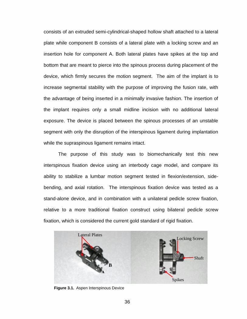
36

consists of an extruded semi-cylindrical-shaped hollow shaft attached to a lateral

plate while component B consists of a lateral plate with a locking screw and an

insertion hole for component A. Both lateral plates have spikes at the top and

bottom that are meant to pierce into the spinous process during placement of the

device, which firmly secures the motion segment. The aim of the implant is to

increase segmental stability with the purpose of improving the fusion rate, with

the advantage of being inserted in a minimally invasive fashion. The insertion of

the implant requires only a small midline incision with no additional lateral

exposure. The device is placed between the spinous processes of an unstable

segment with only the disruption of the interspinous ligament during implantation

while the supraspinous ligament remains intact.

The purpose of this study was to biomechanically test this new

interspinous fixation device using an interbody cage model, and compare its

ability to stabilize a lumbar motion segment tested in flexion/extension, side-

bending, and axial rotation. The interspinous fixation device was tested as a

stand-alone device, and in combination with a unilateral pedicle screw fixation,

relative to a more traditional fixation construct using bilateral pedicle screw

fixation, which is considered the current gold standard of rigid fixation.

Lateral Plates Locking Screw

Spikes

A

B

Shaft

Figure 3.1. Aspen Interspinous Device

37

3.3 Methods

Seven fresh, frozen cadaveric human spines from T12 to Sacrum (5 male,

2 female, mean age, 50 years, range: 26 – 64 years) were used in this study.

Each specimen was dissected to remove all non-ligamentous soft tissue while

preserving the vertebral bodies, discs, facet joint capsules and the following

ligamentous soft tissues – anterior longitudinal ligament (ALL), posterior

longitudinal ligament (PLL), the interspinous and the supraspinous ligament.

Prior to testing, the specimen was assessed for any significant structural defects

or anatomical abnormalities through visual inspection and computer tomography

(CT).

An industrial robot (KUKA, GmbH, Augsburg, Germany) was used as the

spine testing apparatus (Figure 2). It applied pure moments on the spinal

segment. A six-axis force-moment sensor (GAMMA, ATI, Apex, NC) was used to

measure the applied load and provide feedback to the robot. The sensor also

measured the off-axis forces and moments in order to provide feedback to

ensure that a pure moment was being applied along the primary axis of motion of

the spine. The robot was programmed using custom force-torque software to

apply three continuous loading and unloading cycles of pure moment in torque

control along each of the primary axis of the spine to simulate flexion-extension

(FE), lateral bending (LB) and axial rotation (AR). The program was set to

minimize loads in all other axes. The relative vertebral motion was captured

using an optoelectronic camera system (Optotrak, Northern Digital Inc.,

Waterloo, Ontario, Canada). The camera system measures the vertebral motion

38

by tracking the relative motion between infra-red markers placed on vertebral

segments.

The coordinate system definition for each vertebrae and set of adjacent

vertebral bodies is based on the ISB 2002 standard7 with one slight modification

regarding the definition of the origin. The ISB standard defines the origin as the

intersection of the proximal and distal y axes in the reference, neutral position. It

requires that the neutral position must be specified, and must be in a position

where the vertebral y axes are coplanar. If the y axes are parallel (do not

intersect at the common origin O) the y axes are constrained to be collinear, and

the origin O is the mid-point between adjacent endplates. Since the vertebral y

axis from one vertebra to another are not guaranteed to be co-planar in a

practical neutral position (i.e. zero load condition) a variation of the standard was

Figure 3.2. Spine Testing Robot with Infra Red markers attached to spine

39

implemented. The axis intersection point was not used and the mid-point

between adjacent endplates was estimated as the midpoint of the two vertebral

origins. Though these points are not guaranteed to be the same, they are likely

close enough and will allow for multiple vertebral kinematics to be calculated

without having to have two origins per vertebra.

Prior to testing, the spine specimens were thawed to room temperature

and then attached to custom-designed spinal fixtures which were made to fix the

spine securely onto the spine testing apparatus. In order to mount the specimen

onto the custom-designed spinal fixture, three pedicle screws were inserted into

the cranial (T12) and caudal vertebra (Sacrum). For the cranial vertebra, two

screws were placed posteriorly through the pedicles into the vertebral body while

the third screw was placed anteriorly through the vertebral body in an anterior-

posterior orientation. A similar approach was applied to the caudal vertebral

(Sacrum) with two screws placed posteriorly at sites that would ensure maximum

bone purchase, and a third screw placed anteriorly through the sacral body.

Stainless steel rods from the testing fixtures were then attached to the pedicle

screws of each end vertebra and fixed using set screws. The rods were secured

onto the spinal fixture using custom-made holders. It was ensured that before

securing the rods onto the spinal fixture, the spine segment (T12 – S) was

positioned in a neutral posture by horizontally orienting the L3 – L4 disc. The

position of the rods and the holders were adjusted depending on the size of the

vertebra. For additional stability, four wood screws were placed into the superior

endplate of the cranial vertebral body and embedded in Cerobend, a liquid metal

40

alloy (HiTech Alloys, Squamish, WA). Similarly, wood screws were inserted onto

the inferior part of the sacral body and embedded in liquid metal alloy. The

intervening discs were left intact and were not entered by screws or

compromised by the potting material.

On the day of testing, the specimen with the custom spinal fixture was

thawed to room temperature and mounted onto the industrial robot. The caudal

spinal fixture was attached to a base pedestal while the cranial fixture was

attached to the robotic arm. (Figure 3). The spine was kept moist using saline

solution. Nondestructive flexibility testing was performed on the specimens using

the robot. The specimens were subjected to three cycles of FE, LB and AR at an

applied pure bending moment of ±5Nm while continuously minimizing off-axis

loads.. Range of motion (ROM) was determined from the third loading cycle for

each specimen. ROM was measured in this study as the angular motion between

the segments at ± 5 Nm. All surgical instrumentation was provided by Lanx,

Broomfield, CO.

Base Pedestal

Custom Fixtures

Figure 3.3. Spine Specimen attached to Custom-fixtures and mounted onto Robot

41

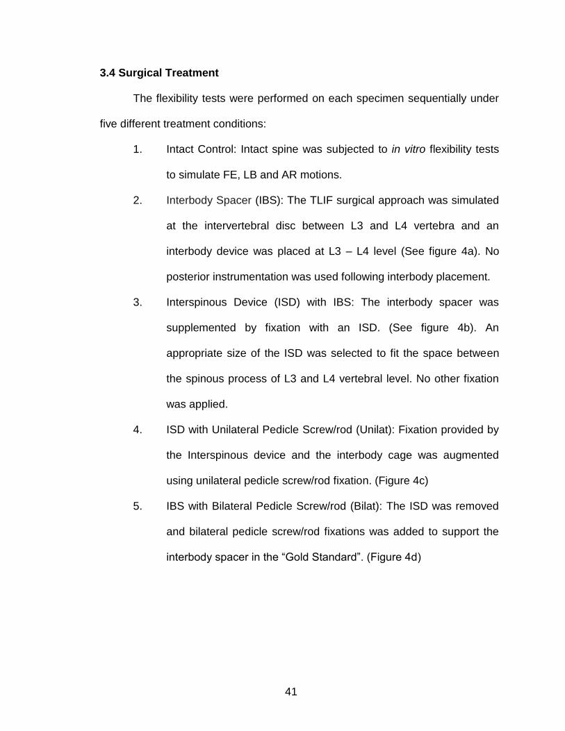
3.4 Surgical Treatment

The flexibility tests were performed on each specimen sequentially under

five different treatment conditions:

1. Intact Control: Intact spine was subjected to in vitro flexibility tests

to simulate FE, LB and AR motions.

2. Interbody Spacer (IBS): The TLIF surgical approach was simulated

at the intervertebral disc between L3 and L4 vertebra and an

interbody device was placed at L3 – L4 level (See figure 4a). No

posterior instrumentation was used following interbody placement.

3. Interspinous Device (ISD) with IBS: The interbody spacer was

supplemented by fixation with an ISD. (See figure 4b). An

appropriate size of the ISD was selected to fit the space between

the spinous process of L3 and L4 vertebral level. No other fixation

was applied.

4. ISD with Unilateral Pedicle Screw/rod (Unilat): Fixation provided by

the Interspinous device and the interbody cage was augmented

using unilateral pedicle screw/rod fixation. (Figure 4c)

5. IBS with Bilateral Pedicle Screw/rod (Bilat): The ISD was removed

and bilateral pedicle screw/rod fixations was added to support the

interbody spacer in the “Gold Standard”. (Figure 4d)

42

Statistical analysis was performed using Minitab 16 (Minitab Inc., State

College, PA). A repeated measures analysis of variance was used to analyze the

ROM between test conditions with a 95% level of significance. Post-hoc Tukey-

Kramer analysis (p < 0.05 was considered statistically significant) was used for

multiple comparisons of the ROM between conditions.

3.5 Results

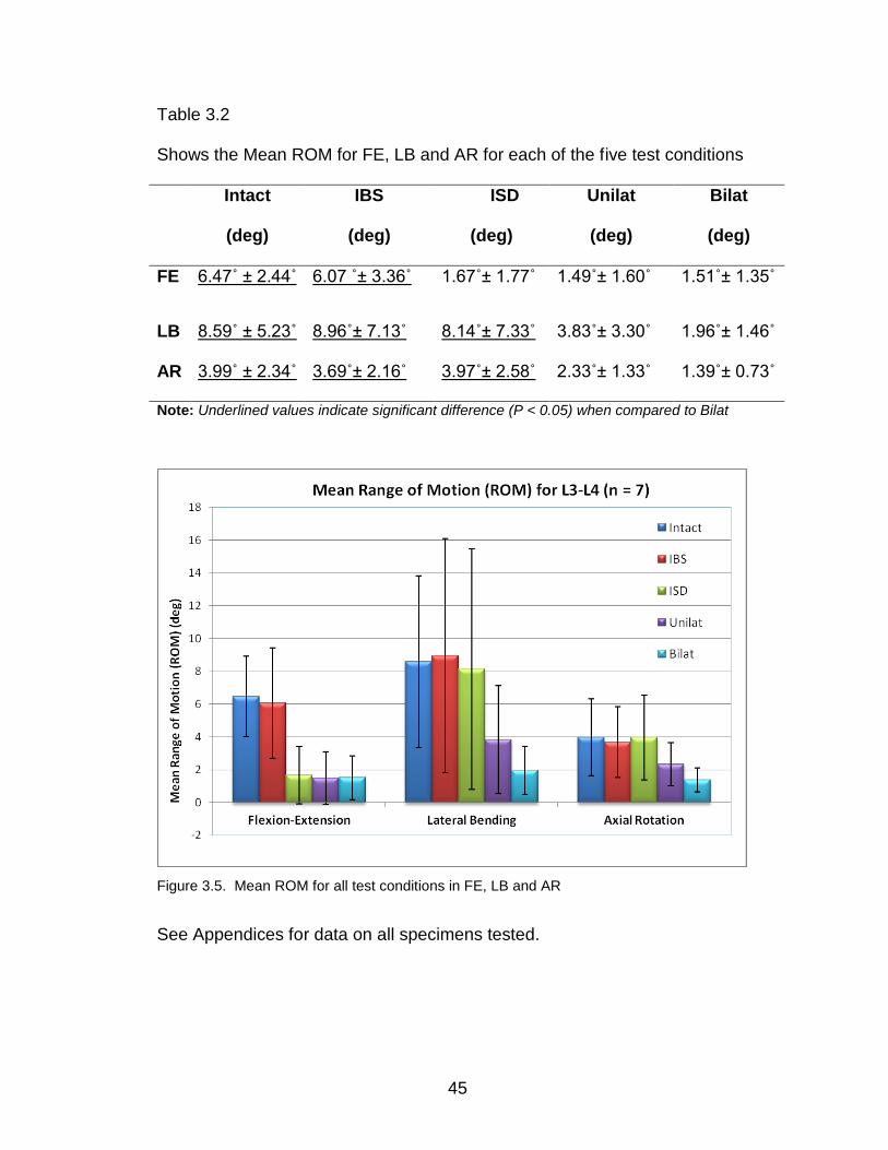
The mean ROM for the intact spine segment was 6.47 ± 2.44˚ in FE, 8.59

± 5.23˚ in LB and 3.99 ± 2.34˚ in AR. Table 1 shows the minimized mean

resultant off-axis forces for FE, LB and AR for each of the five different test

conditions. The IBS placement resulted in a 6% and 7% reduction in ROM in FE

(4a) IBS (4b) ISD (IBS+ISD)

(4d) Bilat: (IBS + Bilateral PS) (4c) Unilat: (IBS+ISD+Unilateral PS)

Figure 3.4. Four Surgical Treatment Conditions

43

and AR, respectively, when compared to the intact control. However the ROM in

LB increased by 4% for IBS group when compared to the control. After additional

implantation of the ISD, a significant decrease in ROM of 74% was observed in

FE. The ISD resulted in a 5% decrease in LB and a 0.4% decrease in AR in

comparison to the intact condition.

The addition of unilateral pedicle screw/rod fixation (Unilat) to ISD/IBS

offered no incremental improvement in FE stiffness, but greatly improved

torsional and side-bending stiffness. The Unilat construct reduced the ROM by

77%, 55% and 42% in FE, LB and AR, respectively, in comparison to intact

controls. The removal of the ISD and the insertion of bilateral pedicle screw/rod

fixation with IBS resulted in a reduction in ROM of 77% in FE, 77% in LB and

65% in AR when compared to the intact control. Figure 5 shows the mean ROM

and standard deviations for the five conditions in the three motion planes, FE, LB

and AR. Table 2 shows the ROM values for all conditions for FE, LB and AR.

A statistical comparison (α = 0.05) between intact control and IBS tests

showed that there was no significant difference in ROM observed in FE (6.47˚±

2.44˚vs 6.07˚± 3.36˚, p = 0.965), LB (8.59˚± 5.23˚vs 8.96˚± 7.13˚, p = 0.770) and

AR (3.99˚± 2.34 vs 3.69˚± 2.16˚, p = 0.982). Comparing the results of the intact to

the ISD group showed that the ISD placement significantly reduced the ROM in

FE (6.47˚± 2.44˚vs 1.67˚± 1.77˚, p < 0.001 however, there were no significant

change in ROM in LB (8.59˚± 5.23˚vs 8.14˚± 7.33˚, p = 0.998) and AR (3.99˚±

2.34˚vs 3.97˚± 2.58˚, p = 0.982).

44

Comparison of the ISD group to the Unilat group showed no significant

change in the ROM in FE (1.67˚± 1.77˚vs 1.49˚± 1.60º, p = 0.998). The

comparison results for LB (8.14˚± 7.33˚vs 3.83˚± 3.30º, p = 0.049) and AR

(3.97˚± 2.58˚vs 2.33˚± 1.33º, p = 0.043), showed that the unilateral pedicle

screw/rod combination significantly reduced the ROM when compared to the ISD

construct alone. A similar trend was observed when comparing the ISD group to

bilateral pedicle screw /rod fixation (Bilat): We found no significant change in FE

ROM (1.67˚± 1.77˚vs 1.51˚± 1.35º, p = 0.998) but a significant reduction in ROM

in the Bilat group in LB (8.14˚± 7.33 ˚vs 1.96˚± 1.46˚, p = 0.002) and AR (3.97˚±

2.58˚vs 1.39˚± 0.73˚, p = 0.001) compared to the ISD alone.

Finally, comparing the results of the Unilat construct to those of the Bilat

fixation construct found no significant difference in FE ROM (1.49˚± 1.60˚vs

1.51˚± 1.35º, p = 1.000), LB (3.83˚± 3.30˚vs 1.96˚± 1.46˚, p = 0.701) and AR

(2.33˚± 1.33˚vs 1.39˚± 0.73º, p = 0.442). Nevertheless, the bilateral pedicle screw

construct showed a trend to be the most rigid construct of all.

Table 3.1

Shows the Mean Resultant off-axis forces for FE, LB and AR for each of the five

test conditions

Intact

(N)

IBS

(N)

ISD

(N)

Unilat

(N)

Bilat

(N)

FE 22.29 ±5.38 25.83± 13.33 25.87 ± 13.52 26.39 ± 14.75 26.39± 15.22

LB 20.08± 6.86 22.51 ± 9.79 24.26 ± 12.74 23.46 ± 12.60 24.11 ± 12.55

AR 13.97 ±2.84 13.72 ± 3.79 12.85 ± 1.66 13.32 ± 2.73 13.86 ± 3.9

45

Table 3.2

Shows the Mean ROM for FE, LB and AR for each of the five test conditions

Intact

(deg)

IBS

(deg)

ISD

(deg)

Unilat

(deg)

Bilat

(deg)

FE 6.47˚ ± 2.44˚ 6.07 ˚± 3.36˚ 1.67˚± 1.77˚ 1.49˚± 1.60˚ 1.51˚± 1.35˚

LB 8.59˚ ± 5.23˚ 8.96˚± 7.13˚ 8.14˚± 7.33˚ 3.83˚± 3.30˚ 1.96˚± 1.46˚

AR 3.99˚ ± 2.34˚ 3.69˚± 2.16˚ 3.97˚± 2.58˚ 2.33˚± 1.33˚ 1.39˚± 0.73˚

Note: Underlined values indicate significant difference (P < 0.05) when compared to Bilat

Figure 3.5. Mean ROM for all test conditions in FE, LB and AR

See Appendices for data on all specimens tested.

46

3.6 Discussion

This study investigated the effect of an interspinous fixation device on the

kinematic behavior of the lumbar spine. The investigated device was designed

for a minimally invasive application involving minimal disruption of structural

elements of the lumbar spine during its implantation. The intended goal is to

provide supplemental support in a TLIF application, obviating the need for

pedicle screw fixation.

The stabilizing effect of the device on the lumbar segment was measured

using in vitro flexibility tests and compared against bilateral pedicle screw

fixation, which may be considered the current gold standard for segmental

fixation of the lumbar spine.8-9 Traditional flexibility tests have, in the past, been

implemented using pulleys and cables to apply static loads, and vertebral

displacements are measured following load application.10-12 Flexibility tests have

also been conducted using specially made fixtures mounted on standard material

testing systems.13-14 However, these test systems tend to constrain the motion of

the spine. More recent spine testing systems involve the use of multi-axis test

systems such as robots which can provide a flexible, repeatable and accurate

way of loading and simulating unconstrained spinal motion. For our study, a

robotic spine testing system was used to apply continuous, unconstrained, pure

moments of ± 5 Nm to the lumbar motion segment to simulate FE, LB and AR.

The test system minimized off-axis forces and moments generated during the

application of load in the primary axis. The uniqueness of our test system, when

compared to other systems in the literature, is in its ability to apply continuous

47

unconstrained pure moments while dynamically optimizing the motion path to

minimize off-axis loads during testing. Our system provides the flexibility to alter

both the loading and boundary conditions of the biomechanical test.

In our study we found that the ROM following the IBS placement, with no

posterior instrumentation in place, was not measurably different from intact

control conditions in any of the motion planes. However, when supplementing the

interbody spacer with the ISD, we observed a significant reduction in FE ROM,

yet motion in LB and AR were not significantly affected when compared to intact.

These results are consistent with those previously presented in the

literature.15-18 Lindsey et al reported that placement of interspinous spacer (X

Stop, SFMT, Concord, CA) at L3 – L4 level significantly reduced ROM in FE with

no effect on the ROM in AR and LB.15 Wilke et al conducted a biomechanical

study on four different interspinous implants and found that all four implants

restricted motion in FE only. They concluded that all the tested implants showed

a similar effect in stabilization in FE while having no effect in LB and AR.16

Karahalios et al conducted a study using this same ISD (Aspen, Lanx,

Broomfield, CO) to supplement an Anterior Lumbar Interbody Fusion (ALIF)

procedure at L4 – L5 level and found a similar trend to our study. They concluded

that the acquired stability was greatest in FE (25% of intact motion retained) and

much less in AR or LB (71% of intact motion was retained for both).17

This study also showed that, in FE, the stability provided by ISD was

statistically equivalent to the unilateral pedicle screw/rod, when used in

combination with the interbody spacer, while in LB and AR, the unilateral pedicle

48

screw/rod construct showed significantly greater stability. We found a similar

trend with bilateral pedicle screw/rod combination when compared to the ISD

alone. In contrast, Karahalios et al found no statistically significant difference in

stability between bilateral pedicle screw fixation and the interspinous devices

used to supplement ALIF in any of the FE, LB and AR tests.17 There are several

reasons for this discrepancy in findings, one of which is the surgical procedures

performed in their study compared to ours (ALIF vs TLIF). Another difference is

in the testing methodology used in their study, the application of load was

dynamically optimized (minimize off axis loads) in our study to ensure

unconstrained pure moment loading conditions throughout the test.

There are few studies currently in the literature that have assessed the

stability provided by unilateral pedicle screw/rod fixation in combination with ISD.

Lo et al developed a finite element model to compare the biomechanical

differences between an ISD and pedicle screw fixation combined with TLIF

against ISD and pedicle screw fixation combined with ALIF. In their study, they

found that the TLIF combination was less stable than the ALIF combination.19

The results from our study showed that additional augmentation of TLIF with

unilateral pedicle screws and ISD was statistically equivalent to TLIF with

bilateral pedicle screws in FE, LB and AR, but that ISD alone was not

comparable.

Only a few animal studies have emerged regarding this new generation of

implants. Bae et al developed a sheep model to assess the interspinous

segmental fusion rate when using an interspinous fixation device. They obtained

49

100% fusion rate when the device was supplemented with bone graft and Bone

Morphogenic Protein (BMP) and a 0% rate of fusion when no BMP was

associated.20 Wang et al compared a small group (21 patients) with interspinous

device (Spire SPP, Medtronic, Minneapolis, MN) used to supplement ALIF, to 11

patients with bilateral pedicle screws. They found no complications, no

pseudoarthrosis and no hardware failure at approximately 5 months of follow up

for both groups.21 However, there are associated complications of using

interspinous devices reported in the literature.22,23 Post-operative spinous

process fracture and device dislocations can both occur with interspinous

devices.22,23

While the ISD studied here did appear to provide suitable fixation to

withstand flexion/extension forces in the patient treated for lumbar fusion, this

study looked at acute fixation strength, and issues of loosening or failure with

protracted cyclic loading were not assessed. Deficiencies in torsional control and

side-bending stiffness are also of concern, as the interbody devices typically

used for TLIF application are inherently weak in these axes as well. Application

of a unilateral pedicle screw construct appears to provide adequate immediate

fixation strength, comparable to the bilateral pedicle screw construct typically

consider a standard, but application of pedicle screws along with the ISD may

negate much of the cost advantage or time/surgical advantage proposed as the

reason for using the interspinous device. Clinical experience to date is limited,

but ongoing studies may provide guidance as to whether supplemental screw are

routinely warranted in adult lumbar fusions using ISD.

50

The adjacent level effects resulting from the implantation of this ISD was

not investigated in this study and could serve as a future study. Clinical data

regarding the use of this ISD is limited and to date no conclusion can be made on

their long term efficacy in promoting fusion.

3.7 Conclusions

The current study assessed the biomechanical stability of the lumbar

spine following a simulated TLIF procedure with an interbody cage alone, the ISD

in combination with the cage, the ISD plus unilateral pedicle screws in

combination with the cage, and bilateral pedicle screws with an interbody cage in

a typical TLIF configuration. We found that the ISD, used to augment the IBS,

was able to provide FE stability comparable to bilateral pedicle screw fixation.

However, it provided minimal stability in LB and AR unless further augmented

with pedicle screws. This study also found that the combination of the ISD with

unilateral pedicle screws was biomechanically equivalent to bilateral pedicle

screws, in providing stability in all directions after a TLIF.

3.8 References

1. Kim KT, Kim YB. Comparison Between Open Procedure and Tubular

Retractor Assisted Procedure for Cervical Radiculopathy: Results of a

Randomized Controlled Study. J Korean Med Sci 2009; 24: 649-53

2. Fessler RG, Khoo LT. Minimally Invasive Cervical Microendoscopic

Foraminotomy: An Initial Clinical Experience. Neurosurgery 51[Suppl

2]:37–45, 2002.

51

3. Anand N, Rosemann R, Khalsa B, Baron EM. Mid-term to long-term

clinical and functional outcomes of minimally invasive correction and

fusion for adults with scoliosis. Neurosurg Focus 28 (3):E6, 2010.

4. Kettler A, Drumm J, Heuer F, Haeussler K, Mack C, Claes L, Wilke HJ.

Can a modified interspinous spacer prevent instability in axial rotation and

lateral bending? A biomechanical in vitro study resulting in a new idea.

Clin Biomech. 2008; 23(2):242-7

5. Böstman O, Myllynen P, Riska EB: Posterior spinal fusion using internal

fixation with the Daab plate. Acta Orthop Scand 55:310–314, 1984.

6. Cobey MC: The value of the Wilson plate in spinal fusion. Clin Orthop

Relat Res 76:138–140, 1971.

7. Wu G, Siegler S, Allard P, Kirtley C, Leardini A, Rosenbaum D, Whittle M,

D'Lima DD, Cristofolini L, Witte H, Schmid O, Stokes I. ISB

recommendation on definitions of joint coordinate system of various joints

for the reporting of human joint motion--part I: ankle, hip, and spine.

International Society of Biomechanics.; Standardization and Terminology

Committee of the International Society of Biomechanics. J Biomech. 2002.

35(4):543-8.

8. Gibson JN, Waddell G. Surgery for degenerative lumbar spondylosis:

Updated Cochrane review. Spine 2005; 30:2312 – 2320

9. Schulte TL,Hurschler C, Haversath M, Liljenqvist U, Bullmann V, Filler TJ,

Osada N, Fallenberg EM, Hackenberg L: The effect of dynamic semi-rigid

52

implants on the range of motion of lumbar motion segments after

decompression. Eur. Spine J 2008; 17: 1057 – 1065

10. Yamamoto I, Panjabi MM, Crisco T, Oxland T. Three-dimensional

movements of the whole lumbar spine and lumbosacral joint.

Spine 1989. 14(11):1256-60.

11. Panjabi M, Dvorak J, Crisco JJ 3rd, Oda T, Wang P, Grob D. Effects of

alar ligament transection on upper cervical spine rotation. J Orthop

Res. 1991 Jul;9(4):584-93.

12. Goel VK, Clark CR, Gallaes K, Liu YK. Moment-rotation relationships of

the ligamentous occipito-atlanto-axial complex. J Biomech. , 1988;

21(8):673-80.

13. Ashman RB, Galpin RD, Corin JD, Johnston CE . Biomechanical analysis

of pedicle screw instrumentation systems in a corpectomy

model.2nd.Spine 1989 Dec;14(12):1398-405.

14. Wilke HJ, Fischer K, Kugler A, Magerl F, Claes L, Wörsdörfer O. In vitro

investigations of internal fixation systems of the upper cervical spine. I.

Stability of the direct anterior screw fixation of the Odontoid. Eur Spine

J. 1992 Dec;1(3):185-90.

15. Lindsey DP, Swanson KE, Fuchs P, Hsu KY, Zucherman JF, Yerby SA.

The Effects of an Interspinous Implant on the Kinematics of the

Instrumented and Adjacent Levels in the Lumbar Spine. Spine 2003.

28(19): 2192– 97

53

16. Wilke HJ, Drumm J, Häussler K, Mack C, Steudel WI, Kettler A.

Biomechanical effect of different lumbar interspinous implants on flexibility

and intradiscal pressure. Eur Spine J. 2008 Aug; 17(8):1049-56.

Epub 2008 Jun 27.

17. Karahalios DG, Kaibara T, Porter RW, et al. Biomechanics of a lumbar

interspinous anchor with anterior lumbar interbody fusion. Laboratory

investigation. J Neurosurg Spine 12:372–380, 2010.

18. Hartmann F, Dietz SO, Hely H, Rommens PM, Gercek E. Biomechanical

effect of different interspinous devices on lumbar spinal range of motion

under preload conditions. Arch Orthop Trauma Surg. 2011; 131(7):917-26.

19. Lo CC, Tsai KJ, Zhong ZC, Chen SH, Hung C. Biomechanical differences

of Coflex-F and pedicle screw fixation combined with TLIF or ALIF - a

finite element study. Comput Methods Biomech Biomed Engin. 2011 Mar

1:1. [Epub ahead of print]

20. Bae H; Ashraf N, Kanim LEA. Evaluation of Interlaminar Lumbar

Instrumented Fusion (ILIF) in a Sheep Model. Abstract 617 from the 17th

IMAST, 2010– Toronto, ON.

21. Wang JC, Haid RW Jr, Miller JS, Robinson JC. Comparison of CD

HORIZON SPIRE spinous process plate stabilization and pedicle screw

fixation after anterior lumbar interbody fusion. Invited submission from the

Joint Section Meeting On Disorders of the Spine and Peripheral Nerves,

March 2005. J Neurosurg Spine. 2006 Feb; 4(2):132-6.

54

22. Kim DH, Tantorski M, Shaw J, Martha J, Li L, Shanti N, Rencu T, Parazin

S, Kwon B. Occult spinous process fractures associated

with interspinous process spacers. Spine 2011. 15;36(16): 1080 - 5.

23. Barbagallo GM, Olindo G, Corbino L, Albanese V. Analysis of

complications in patients treated with the X-Stop Interspinous Process

Decompression System: proposal for a novel anatomic scoring system for

patient selection and review of the literature. Neurosurgery. 2009

Jul;65(1):111-19; discussion 119-20.

55

CHAPTER IV

HYBRID DYNAMIC STABILIZATION: A BIOMECHANICAL ASSESSMENT OF

ADJACENT AND SUPRA-ADJACENT LEVELS

(Submitted for publication – Journal of Neurosurgery: Spine)

4.1 Abstract

The primary goal of this study was to use the developed biomechanical

testing methodology involving the robotic system to access and evaluate a hybrid

dynamic stabilization system and its effect on adjacent level motion.

4.1.1 Study design. A human spine cadaveric study accessing the

biomechanical effects of pedicle screw based dynamic stabilization of the supra

adjacent level to a one level lumbar fusion.

Objective: To evaluate the effect of hybrid dynamic stabilization on adjacent

levels of lumbar spine.

4.1.2 Summary of background. One of the many proposed indications

for dynamic stabilization is its use as transition instrumentation adjacent to a solid

fusion to protect that adjacent level from excessive compensating motion / stress

and also aid in creating a smoother motion transition to the other levels of the

spine. In this model, we accessed the angular range of motion (ROM) of the

adjacent levels of the spine after a L4 - L5 instrumented fusion. Subsequently,

56

we implanted a pedicle screw dynamic stabilization device at L3 - L4 and

analyzed biomechanically its protective effects on that level as well as the ROM

on the remaining segments of the lumbar spine.

4.1.3 Methods. Seven human specimens T12-sacrum were used. The

following conditions were implemented: (1) Intact spine, (2) Fusion of L4-5 with

bilateral pedicle screws and titanium rods, and (3) Supplementation of the L4-5

fusion with a pedicle screw dynamic stabilization construct (Zimmer, Warsaw, IN)

at L3-L4, with the purpose of protecting the L3-4 level from the excessive ROM

and also to create a smoother motion transition to the rest of the lumbar spine.

The robot applied continuous pure moment (±2 Nm) in flexion-extension (FE)

with and without follower load, lateral bending (LB) and axial rotation (AR).

Intersegmental rotations of the fused, dynamically stabilized and adjacent levels

were measured and compared.

4.1.4 Results. The rigid instrumentation at L4 – L5 caused a 78%

decrease in the segment’s F/E when compared to the intact specimen. To

compensate, it caused an increase in motion at L1 – L2 (45.6%) and L2 – L3

(23.2%) (P = 0.00). No statistically significant increase in the ROM was seen at

T12-1, L3-4 or L5-S1. The placement of the dynamic construct at L3 – L4,

decreased the operated level’s motion by 80.4% (same stability as the fusion at

L4-5) and caused a significant increase in motion at all tested adjacent levels:

T12 – L1 (73.4%), L1 – L2 (85.0%), L2 – L3 (49.9%) and L5 – S1 (20.8%).

In FE with follower load, instrumentation at L4 – L5 showed no significant

change in motion at all adjacent levels except L5 – S1 which showed a significant

57

increase in motion of 52.0%. There was a significant reduction in motion at the

operated level, L4 – L5 (76.4%). The addition of a dynamic construct caused a

significant decrease in motion at the operated level, L3 – L4 (76.7% - very similar

stability found at the adjacent lower fused level), while the adjacent levels, T12 –

L1 (44.9%), L1 – L2 (57.3%) and L5 – S1 (83.9%) all showed a significant

increase in motion. The only exception was L2 – L3 with no significant change in

ROM.

In LB, instrumentation at L4 – L5, showed no significant change in motion

in all the adjacent levels except T12 – L1 (increase of 22.8%). The operated

level, L4 – L5, showed a decrease in motion of 83.6% when compared to intact.

The placement of the dynamic construct at L3 – L4 after the L4 - L5 fusion

caused an increase in motion at T12 – L1 (69.9%), L1 – L2 (59.4%), L2 – L3

(44.7%), L5 – S1 (43.7%) and a significant decrease in motion of 80.7% at the

operated level, L3 – L4.

In AR, there were no significant changes in motion at the adjacent levels

after L4 – L5 fusion. The operated level, L4 – L5 showed a decrease in motion of

46.1%. The placement of dynamic construct at L3 – L4 after the L4-5 fusion

caused a significant increase in motion of the adjacent levels, L2 – L3 (25.1%)

and L5 – S1 (31.4%). There was a significant decrease in motion of 38% at the

operated level, L3 – L4.

4.1.5 Conclusion. The dynamic stabilization system had the same

stability as a solid all metal construct. Its addition to the supra adjacent level (L3-

L4) to the fusion (L4- L5) in deed protected the adjacent level from excessive

58

motion. However, it essentially transformed a 1 level into a 2 level lumbar fusion

with exponential transfer of motion to the fewer remaining discs.

4.2 Introduction

Intervertebral fusion is considered the gold standard for the treatment of

lumbar segmental instability which is typically caused by degeneration of the

intervertebral disc, zygapophysical joints and ligaments [1-2]. However, studies

have shown that fusion causes accelerated degeneration at adjacent levels. [3-

13]. This has led to the development of motion-preserving treatment options as

an alternative to fusion. [2,14]. One of such options is Dynamic stabilization. It

involves the use of a semi-rigid implant design to stabilize a dysfunctional lumbar

spinal segment. It is intended to mitigate accelerated adjacent level degeneration

and limit abnormal motion which contributes to disc and ligamentous

degeneration. Dynamic stabilization may be implemented as a stand-alone

technique or as a hybrid technique. In a stand-alone application, the injured or

degenerated segment is instrumented posteriorly only with a dynamic system, in

the hope that the system’s stabilizing properties will be sufficient to prevent

dysfunctional segmental motion; no fusion is performed, reducing the risk of

subsequent degeneration at adjacent levels. In the hybrid application, a fusion is

performed at the injured or degenerated segment using rigid implants applied

posteriorly, with dynamic stabilization extended to levels above or below the

segment to be fused (Topping off). The goal of a hybrid application is to

prophylactically limit stress at the level above or below the fusion and prevent the

development of adjacent level disease.

59

Several clinical studies have focused on dynamic stabilization as a stand-

alone alternative to traditional fusion. Kim et. al. conducted a 3 year follow-up

post-op study on 21 patients who underwent lumbar spinal stabilization with

dynamic stabilization and found a significant decrease in range of motion (ROM)

at the operated level and a significant increase in motion at the adjacent

levels.[15]. Cakir et al performed an in vivo study of 26 patients with degenerative

instability who underwent decompression and stand-alone dynamic stabilization

versus decompression and standard fusion. Patients who underwent fusion

demonstrated decreased global and segmental ROM, while patients who

underwent dynamic stabilization demonstrated preserved global and segmental

ROM. In both groups, adjacent level ROM was unchanged when compared with

the pre-operative state. [16]. Kumar et al performed dynamic stabilization in 32

patients, using both stand-alone (20 patients) and hybrid (12 patients)

procedures. Follow-up was performed with 2 year post-op MRI scans; clinical

outcomes were not assessed. In patients who received a hybrid procedure, the

unfused, dynamically-stabilized segments demonstrated evidence of additional

degeneration in 25% of patients, and the segment above the dynamically

stabilized segment demonstrated additional degeneration in 8%. However,

interpretation of these hybrid results is limited by the small number of patients

involved and the subjective nature of the primary outcome measure. [17].

Presently, there is a lack of biomechanical data supporting the hybrid

application of dynamic systems. In particular, there is a lack of information

regarding the effect of hybrid stabilization on the levels above the dynamically

60

stabilized level. It is possible that dynamic stabilization above a fusion will simply

transmit stresses created by the fusion to the motion segment above the dynamic

stabilization, accelerating degeneration over a longer segment of the spine. The

aim of this study was to analyze the effect of the hybrid dynamic stabilization

system on the ROM of the lumbar segments, adjacent to the operated level.

4.3 Materials and Methods

4.3.1 Specimen Preparation. Seven fresh, frozen cadaveric human

spines from T12 to Sacrum (6 male, 1 female, mean age, 60 years, range: 37 –

69 years) were used in this study. Each specimen was dissected to remove all

non-ligamentous soft tissue while preserving the vertebral bodies, discs, facet

joint capsules and the following ligamentous soft tissues – anterior longitudinal

ligament (ALL), posterior longitudinal ligament (PLL), the interspinous and the

supraspinous ligament. The spine was then frozen at -20˚ C until testing. Prior to

testing, the specimen was assessed for any significant structural defects or

anatomical abnormalities through visual inspection and computer tomography

(CT).

The spine was thawed to room temperature overnight prior to test day and

it was ensured that the spine was kept moist during testing by lightly spraying

exposed tissues using saline solution. Custom-designed spinal fixtures were

made to fix the spine securely onto the spine testing apparatus. In order to mount

the specimen onto the spinal fixture, three pedicle screws were inserted into the

cranial (T12) and caudal vertebra (Sacrum).

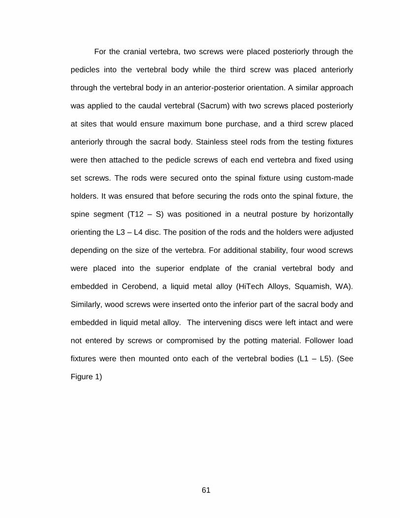
61

For the cranial vertebra, two screws were placed posteriorly through the

pedicles into the vertebral body while the third screw was placed anteriorly

through the vertebral body in an anterior-posterior orientation. A similar approach

was applied to the caudal vertebral (Sacrum) with two screws placed posteriorly

at sites that would ensure maximum bone purchase, and a third screw placed

anteriorly through the sacral body. Stainless steel rods from the testing fixtures

were then attached to the pedicle screws of each end vertebra and fixed using

set screws. The rods were secured onto the spinal fixture using custom-made

holders. It was ensured that before securing the rods onto the spinal fixture, the

spine segment (T12 – S) was positioned in a neutral posture by horizontally

orienting the L3 – L4 disc. The position of the rods and the holders were adjusted

depending on the size of the vertebra. For additional stability, four wood screws

were placed into the superior endplate of the cranial vertebral body and

embedded in Cerobend, a liquid metal alloy (HiTech Alloys, Squamish, WA).

Similarly, wood screws were inserted onto the inferior part of the sacral body and

embedded in liquid metal alloy. The intervening discs were left intact and were

not entered by screws or compromised by the potting material. Follower load

fixtures were then mounted onto each of the vertebral bodies (L1 – L5). (See

Figure 1)

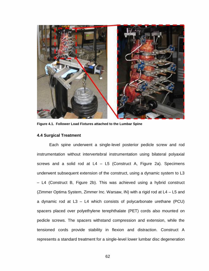
62

Figure 4.1. Follower Load Fixtures attached to the Lumbar Spine

4.4 Surgical Treatment

Each spine underwent a single-level posterior pedicle screw and rod

instrumentation without intervertebral instrumentation using bilateral polyaxial

screws and a solid rod at L4 – L5 (Construct A, Figure 2a). Specimens

underwent subsequent extension of the construct, using a dynamic system to L3

– L4 (Construct B, Figure 2b). This was achieved using a hybrid construct

(Zimmer Optima System, Zimmer Inc. Warsaw, IN) with a rigid rod at L4 – L5 and

a dynamic rod at L3 – L4 which consists of polycarbonate urethane (PCU)

spacers placed over polyethylene terephthalate (PET) cords also mounted on

pedicle screws. The spacers withstand compression and extension, while the

tensioned cords provide stability in flexion and distraction. Construct A

represents a standard treatment for a single-level lower lumbar disc degeneration

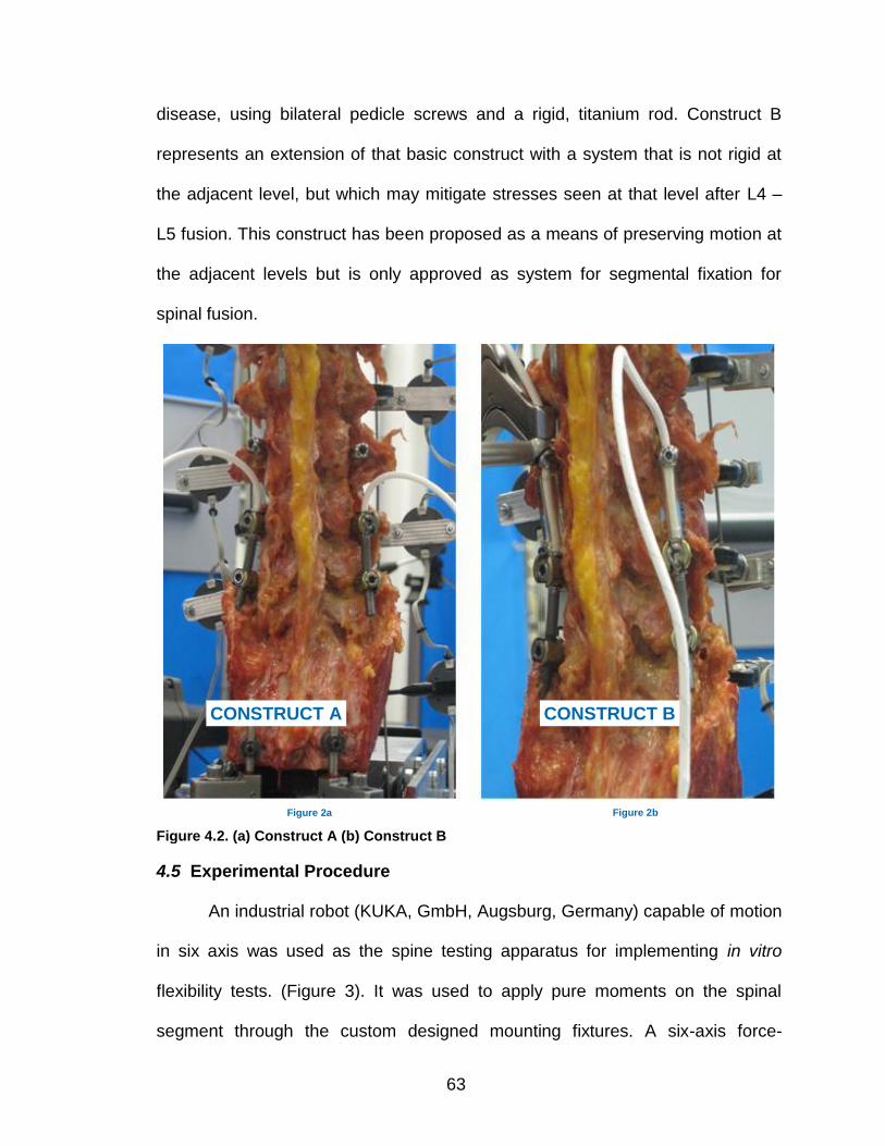
63

disease, using bilateral pedicle screws and a rigid, titanium rod. Construct B

represents an extension of that basic construct with a system that is not rigid at

the adjacent level, but which may mitigate stresses seen at that level after L4 –

L5 fusion. This construct has been proposed as a means of preserving motion at

the adjacent levels but is only approved as system for segmental fixation for

spinal fusion.

4.5 Experimental Procedure

An industrial robot (KUKA, GmbH, Augsburg, Germany) capable of motion

in six axis was used as the spine testing apparatus for implementing in vitro

flexibility tests. (Figure 3). It was used to apply pure moments on the spinal

segment through the custom designed mounting fixtures. A six-axis force-

CONSTRUCT A

Figure 2a

CONSTRUCT B

Figure 2b

Figure 4.2. (a) Construct A (b) Construct B

64

moment sensor (GAMMA, ATI, Apex, NC) was used to measure the applied load

and provide feedback for the robot. The sensor was also used to measure the

off-axis forces and moments in order provide feedback to ensure that a pure

moment was being applied along the primary axis of motion of the spine.

The robot was programmed using its custom force-torque software to

apply three continuous loading and unloading cycles of pure moment in force

control along each of the primary axis of the spine to simulate flexion-extension

(FE), flexion-extension with a follower load of 600 N (FE-FL), lateral bending (LB)

Figure 4.3. Spine Testing Robot

65

and Axial rotation (AR). Throughout the test, kinematics and kinetics of the

refined center of rotation point are recorded at 83Hz. The specimens were pre-

conditioned to eliminate any viscoelastic effects. ROM was determined from the

third loading cycle for each specimen under each of the test conditions (intact,

construct A, construct B). The relative vertebral motion was captured using an

optoelectronic camera system (Optotrak, Northern Digital Inc., Waterloo, Ontario,

Canada). The camera system measures the vertebral motion by tracking the

relative motion between infra-red markers placed on each vertebral segment,

T12 – S.

The hybrid test protocol originally developed by Panjabi et al was used to

assess the effect of the placement of Construct A and Construct B on the

adjacent level segments. [8 – 11]. The protocol was a two part process;

1. An intact flexibility test was conducted to determine the ROM of the

intact specimen under pure moments of ± 2 Nm in FE, FL-FE, LB

and AR.

2. Following the placement of the constructs, the specimen was

subjected to pure moments until the ROM of the constructs equaled

the intact ROM for FE, FE-FL, LB and AR. A unique feature of the

robotic system was in its ability to follow the same rotational

trajectory obtained from the intact test above, in other words,

following the placement of the constructs, the spine was forced to

follow the same rotational trajectory as the intact in reaching the

intact ROM.

66

4.6 Data and Statistical Analysis

In order to study the effect of both Construct A and Construct B treatments

on the adjacent levels, a nondimensional parameter, adjacent level effects (ALE),

was determined (Panjabi et. al, 2007). ALE can be defined as the normalized

(Intact) percentage difference between ROM following treatment and ROM at

intact. The ALE at each adjacent level was given by the formula:

ALE (%) = 100 X (iROMtreatment – iROMintact)/ iROMintact

where iROMtreatment = intervertebral motion after Construct A or Construct

B placement

iROMintact = intact intervertebral motion

Statistical analysis was performed using Minitab 16 (Minitab Inc., State

College, PA). A repeated measures analysis of variance was used to compare

the segmental ROM after surgical treatment with the intact segmental ROM.

Post-hoc Tukey-Kramer analysis (P < 0.05 was considered statistically

significant) was used for multiple comparisons.

4.7 Results

4.7.1 Flexion-extension. Table 1 shows the intervertebral range of

motion for the intact, Construct A and Construct B treatment conditions for

flexion-extension. Figure 4 shows the average intervertebral range of motion for

Intact, Construct A and Construct B for flexion-extension. In flexion-extension,

Construct A at L4 – L5 caused no significant change in motion at the following

adjacent levels when compared to intact: L3 – L4 (P = 0.36) and L5 – S (P =

0.76). However, there was a 30.9% increase in motion at T12 – L1 (P = 0.05),

67

45.6% increase in motion at L1 – L2 (P < 0.001) and a 23.2% increase in motion

at L2 – L3 (P = 0.03). There was a significant decrease in motion of 78% when

compared to intact at L4 – L5 following placement of Construct A. (P < 0.001).

The placement of Construct B at L3 – L4, decreased the motion by -80.4% at the

operated level and caused a significant increase in motion at the adjacent levels,

T12 – L1 (73.4%), L1 – L2 (85.0%), L2 – L3 (49.9%) and L5 – S (20.8%). There

was no significant change in motion at L4 – L5 (1.03 ± 0.51 vs 1.24 ± 0.83, P =

0.92) with the addition of Construct B. The graphical representation of the

distribution of motion (ALE) to the adjacent levels after Construct A and

Construct B placement can be clearly seen for flexion-extension (Figure 5). The

results show that placement of both Construct A and Construct B causes a

substantial increase in ALE of non-operated levels with Construct B producing

the larger increase of the two constructs.

4.7.2 Flexion-extension with follower load. Table 2 shows the

intervertebral range of motion for the intact, Construct A and Construct B for

flexion-extension with follower load. Figure 6 shows the average intervertebral

range of motion for Intact, Construct A and Construct B for flexion-extension with

follower load. In flexion-extension with follower load, placement of Construct A at

L4 – L5 showed no significant change in motion at T12 – L1 (P = 0.08), L1 – L2

(P = 0.34), L2 – L3 (P = 0.11) and L3 – L4 (P = 0.87) when compared to intact.

However, there was a significant increase in motion of 52.0% at L5 – S (P <

0.001) when compared to intact. There was a significant reduction in motion at

the operated level, L4 – L5 (-76.4%) following Construct A placement. (P =

68

.0008). The placement of Construct B, caused a significant decrease in motion at

the operated level, L3 – L4 (-76.7%) while the adjacent levels, T12 – L1 (44.9%),

L1 – L2 (57.3%) and L5 – S (83.9%) all showed a significant increase in motion

except L2 – L3 which showed no significant change in motion. (P = 0.11). The

ALE results for flexion-extension with follower load are shown in Figure 7. The

addition of Construct A and Construct B resulted in a larger increase in ALE to

the sub-adjacent non-operated level (L5 – S) when compared to flexion-

extension.

4.7.3 Lateral bending. Table 3 shows the intervertebral range of motion

for the intact, Construct A and Construct B for lateral bending. Figure 8 shows

the average intervertebral range of motion for Intact, Construct A and Construct

B for Lateral Bending. In lateral bending, for Construct A at L4 – L5, the results

showed that there was no significant change in motion in all the adjacent levels

except T12 – L1 which showed an increase in motion of 22.8%. The L4 – L5 level

(Construct A), showed a decrease in motion of -83.6% when compared to intact.

The placement of the Construct B at L3 – L4 caused an increase in motion at

T12 – L1 (69.9%), L1 – L2 (59.4%), L2 – L3 (44.7%) and L5 – S (43.7%). There

was a significant decrease in motion of -80.7% at L3 – L4 after Construct B

placement. A visual representation of ALE is shown in Figure 9 for lateral

bending with Construct B causing a larger change in ALE on the non-operated

levels compared to Construct A.

4.7.4 Axial rotation. Table 4 shows the intervertebral range of motion for

the intact, fusion Construct A and Construct B for axial rotation. Figure 10 shows

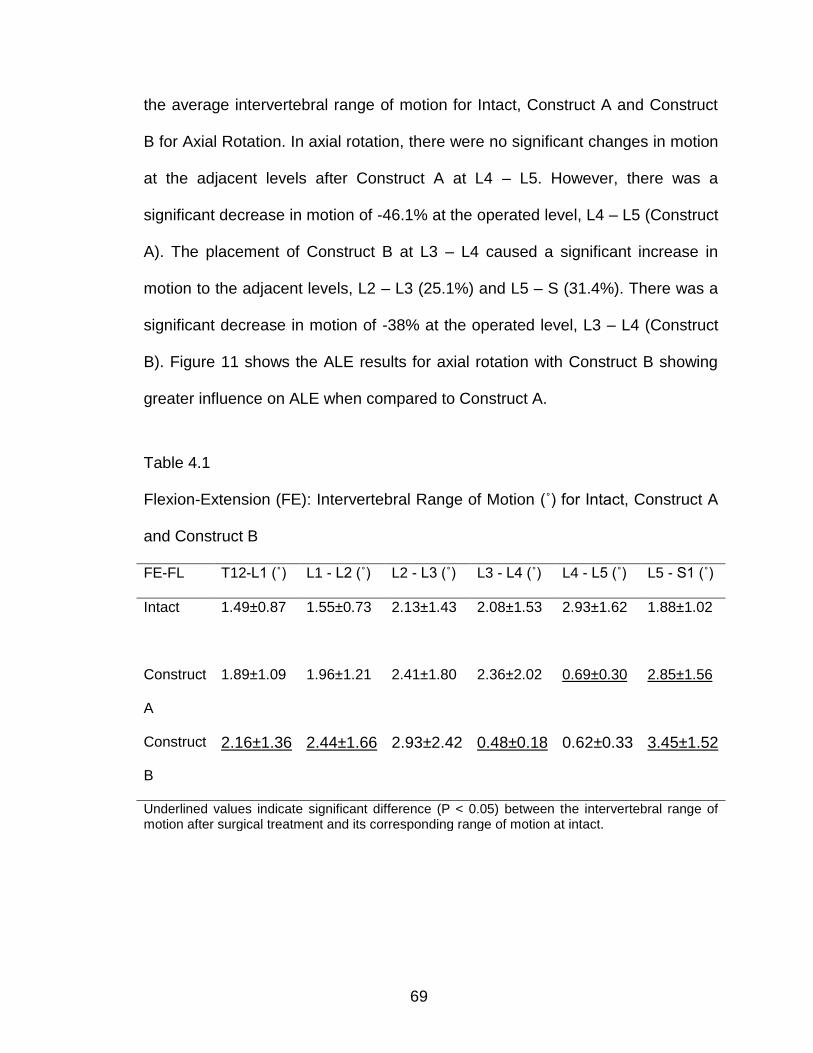
69

the average intervertebral range of motion for Intact, Construct A and Construct

B for Axial Rotation. In axial rotation, there were no significant changes in motion

at the adjacent levels after Construct A at L4 – L5. However, there was a

significant decrease in motion of -46.1% at the operated level, L4 – L5 (Construct

A). The placement of Construct B at L3 – L4 caused a significant increase in

motion to the adjacent levels, L2 – L3 (25.1%) and L5 – S (31.4%). There was a

significant decrease in motion of -38% at the operated level, L3 – L4 (Construct

B). Figure 11 shows the ALE results for axial rotation with Construct B showing

greater influence on ALE when compared to Construct A.

Table 4.1

Flexion-Extension (FE): Intervertebral Range of Motion (˚) for Intact, Construct A

and Construct B

FE-FL T12-L1 (˚) L1 - L2 (˚) L2 - L3 (˚) L3 - L4 (˚) L4 - L5 (˚) L5 - S1 (˚)

Intact 1.49±0.87

1.55±0.73 2.13±1.43 2.08±1.53 2.93±1.62 1.88±1.02

Construct

A

1.89±1.09 1.96±1.21 2.41±1.80 2.36±2.02 0.69±0.30 2.85±1.56

Construct

B

2.16±1.36 2.44±1.66 2.93±2.42 0.48±0.18 0.62±0.33 3.45±1.52

Underlined values indicate significant difference (P < 0.05) between the intervertebral range of motion after surgical treatment and its corresponding range of motion at intact.

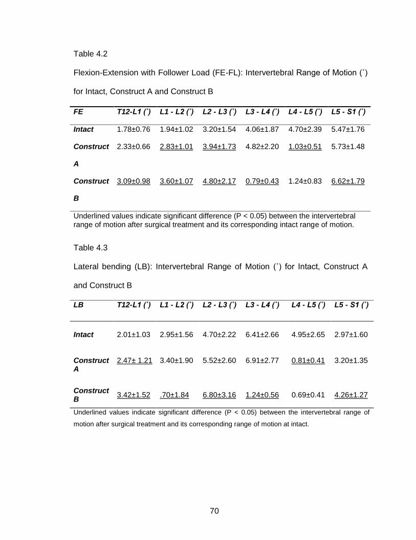
70

Table 4.2

Flexion-Extension with Follower Load (FE-FL): Intervertebral Range of Motion (˚)

for Intact, Construct A and Construct B

Table 4.3

Lateral bending (LB): Intervertebral Range of Motion (˚) for Intact, Construct A

and Construct B

FE T12-L1 (˚) L1 - L2 (˚) L2 - L3 (˚) L3 - L4 (˚) L4 - L5 (˚) L5 - S1 (˚)

Intact 1.78±0.76 1.94±1.02 3.20±1.54 4.06±1.87 4.70±2.39 5.47±1.76

Construct

A

2.33±0.66 2.83±1.01 3.94±1.73 4.82±2.20 1.03±0.51 5.73±1.48

Construct

B

3.09±0.98 3.60±1.07 4.80±2.17 0.79±0.43 1.24±0.83 6.62±1.79

Underlined values indicate significant difference (P < 0.05) between the intervertebral range of motion after surgical treatment and its corresponding intact range of motion.

LB T12-L1 (˚) L1 - L2 (˚) L2 - L3 (˚) L3 - L4 (˚) L4 - L5 (˚) L5 - S1 (˚)

Intact 2.01±1.03

2.95±1.56

4.70±2.22

6.41±2.66

4.95±2.65

2.97±1.60

Construct A

2.47± 1.21

3.40±1.90

5.52±2.60

6.91±2.77

0.81±0.41

3.20±1.35

Construct B

3.42±1.52

.70±1.84

6.80±3.16

1.24±0.56

0.69±0.41

4.26±1.27

Underlined values indicate significant difference (P < 0.05) between the intervertebral range of

motion after surgical treatment and its corresponding range of motion at intact.

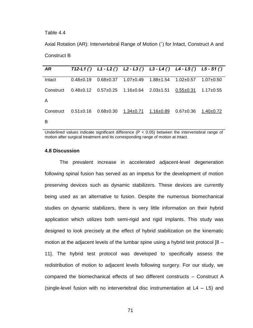
71

Table 4.4

Axial Rotation (AR): Intervertebral Range of Motion (˚) for Intact, Construct A and

Construct B

4.8 Discussion

The prevalent increase in accelerated adjacent-level degeneration

following spinal fusion has served as an impetus for the development of motion

preserving devices such as dynamic stabilizers. These devices are currently

being used as an alternative to fusion. Despite the numerous biomechanical

studies on dynamic stabilizers, there is very little information on their hybrid

application which utilizes both semi-rigid and rigid implants. This study was

designed to look precisely at the effect of hybrid stabilization on the kinematic

motion at the adjacent levels of the lumbar spine using a hybrid test protocol [8 –

11]. The hybrid test protocol was developed to specifically assess the

redistribution of motion to adjacent levels following surgery. For our study, we

compared the biomechanical effects of two different constructs – Construct A

(single-level fusion with no intervertebral disc instrumentation at L4 – L5) and

AR T12-L1 (˚) L1 - L2 (˚) L2 - L3 (˚) L3 - L4 (˚) L4 - L5 (˚) L5 - S1 (˚)

Intact 0.48±0.19 0.68±0.37 1.07±0.49 1.88±1.54 1.02±0.57 1.07±0.50

Construct

A

0.48±0.12 0.57±0.25 1.16±0.64 2.03±1.51 0.55±0.31 1.17±0.55

Construct

B

0.51±0.16 0.68±0.30 1.34±0.71 1.16±0.89 0.67±0.36 1.40±0.72

Underlined values indicate significant difference (P < 0.05) between the intervertebral range of motion after surgical treatment and its corresponding range of motion at intact.

72

Construct B (Stabilization of adjacent level, L3 – L4 using hybrid dynamic

stabilization with no intervertebral disc instrumentation) on the adjacent non-

operated levels.

Traditional flexibility tests, have in the past, been implemented using

pulleys and cables to apply the loads and generally vertebral motion

measurements are taken statically following load application [18 - 20]. For our

study, in implementing the hybrid test protocol, a robotic spine testing system

was used to apply continuous unconstrained pure moment of ± 2 Nm on the

lumbar motion segment to simulate FE, LB and AR. The test system minimized

off-axis forces and moments generated during the application of load in the

primary axis. The uniqueness of our test system, when compared to other

systems in the literature is in its ability to apply continuous unconstrained pure

moment while dynamically optimizing the motion path to minimize off axis loads

during testing. The test system enables precise control over the loading and

boundary conditions of the test over the entire test duration, thus ensuring test

reliability and reproducibility. In implementing the hybrid test, our system also has

the unique feature of enabling the treated spine to follow the same rotational

trajectory obtained from the intact spine.

In our study, we found that placement of Construct B caused an overall

higher increase in ALE than Construct A in all the test conditions (flexion-

extension, flexion-extension with follower-load, lateral bending and axial rotation).

In assessing the effect of each construct separately on the adjacent levels for

flexion-extension, we found that Construct A caused no significant increase in

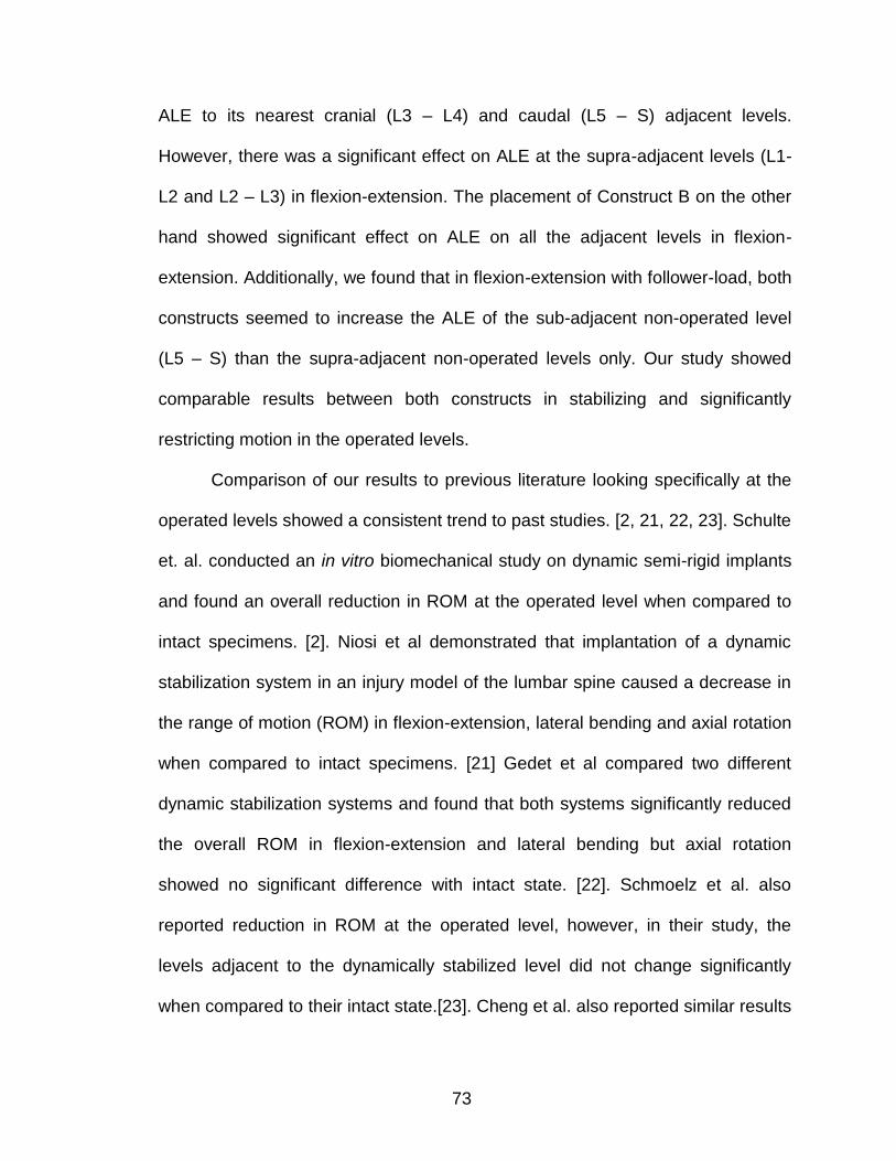
73

ALE to its nearest cranial (L3 – L4) and caudal (L5 – S) adjacent levels.

However, there was a significant effect on ALE at the supra-adjacent levels (L1-

L2 and L2 – L3) in flexion-extension. The placement of Construct B on the other

hand showed significant effect on ALE on all the adjacent levels in flexion-

extension. Additionally, we found that in flexion-extension with follower-load, both

constructs seemed to increase the ALE of the sub-adjacent non-operated level

(L5 – S) than the supra-adjacent non-operated levels only. Our study showed

comparable results between both constructs in stabilizing and significantly

restricting motion in the operated levels.

Comparison of our results to previous literature looking specifically at the

operated levels showed a consistent trend to past studies. [2, 21, 22, 23]. Schulte

et. al. conducted an in vitro biomechanical study on dynamic semi-rigid implants

and found an overall reduction in ROM at the operated level when compared to

intact specimens. [2]. Niosi et al demonstrated that implantation of a dynamic

stabilization system in an injury model of the lumbar spine caused a decrease in

the range of motion (ROM) in flexion-extension, lateral bending and axial rotation

when compared to intact specimens. [21] Gedet et al compared two different

dynamic stabilization systems and found that both systems significantly reduced

the overall ROM in flexion-extension and lateral bending but axial rotation

showed no significant difference with intact state. [22]. Schmoelz et al. also

reported reduction in ROM at the operated level, however, in their study, the

levels adjacent to the dynamically stabilized level did not change significantly

when compared to their intact state.[23]. Cheng et al. also reported similar results

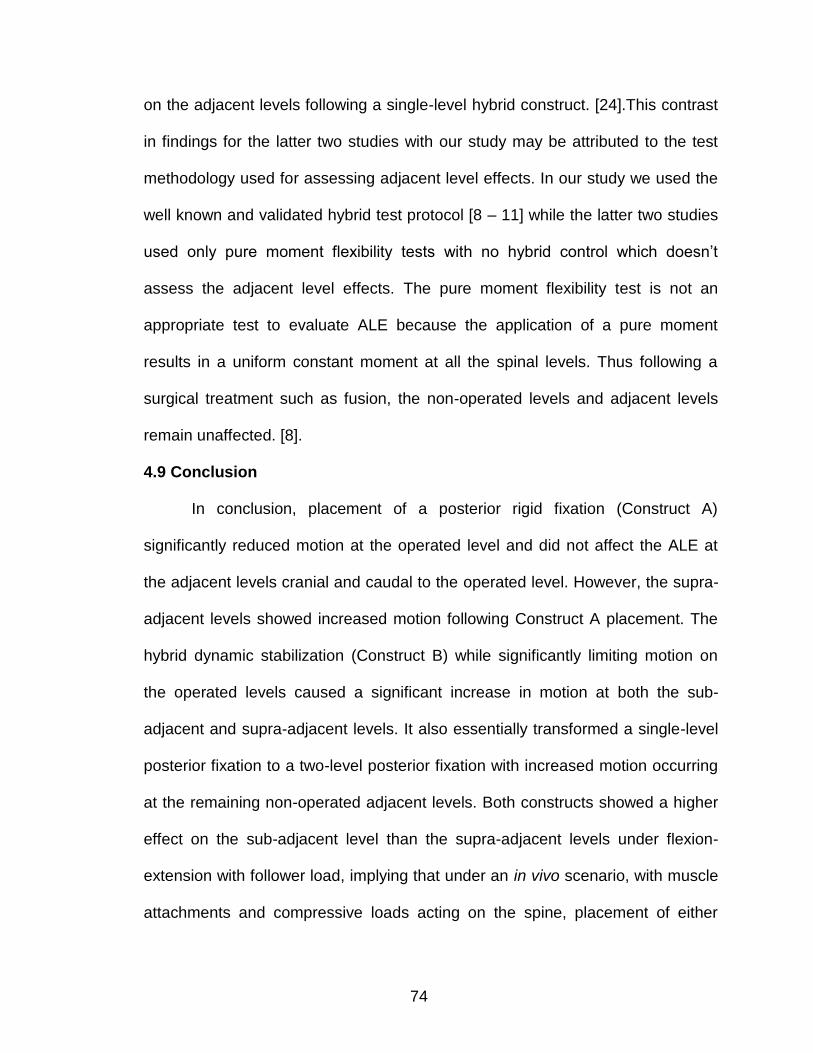
74

on the adjacent levels following a single-level hybrid construct. [24].This contrast

in findings for the latter two studies with our study may be attributed to the test

methodology used for assessing adjacent level effects. In our study we used the

well known and validated hybrid test protocol [8 – 11] while the latter two studies

used only pure moment flexibility tests with no hybrid control which doesn’t

assess the adjacent level effects. The pure moment flexibility test is not an

appropriate test to evaluate ALE because the application of a pure moment

results in a uniform constant moment at all the spinal levels. Thus following a

surgical treatment such as fusion, the non-operated levels and adjacent levels

remain unaffected. [8].

4.9 Conclusion

In conclusion, placement of a posterior rigid fixation (Construct A)

significantly reduced motion at the operated level and did not affect the ALE at

the adjacent levels cranial and caudal to the operated level. However, the supra-

adjacent levels showed increased motion following Construct A placement. The

hybrid dynamic stabilization (Construct B) while significantly limiting motion on

the operated levels caused a significant increase in motion at both the sub-

adjacent and supra-adjacent levels. It also essentially transformed a single-level

posterior fixation to a two-level posterior fixation with increased motion occurring

at the remaining non-operated adjacent levels. Both constructs showed a higher

effect on the sub-adjacent level than the supra-adjacent levels under flexion-

extension with follower load, implying that under an in vivo scenario, with muscle

attachments and compressive loads acting on the spine, placement of either

75

construct would to a certain degree affect the sub-adjacent level more than the

supra-adjacent level.

Figure 4.5. ALE results for Flexion-Extension

Figure 4.4. Mean ROM for Flexion-Extension

76

Figure 4.6. Flexion-Extension with Follower Load

Figure 4.7. ALE results for Flexion-Extension with Follower Load

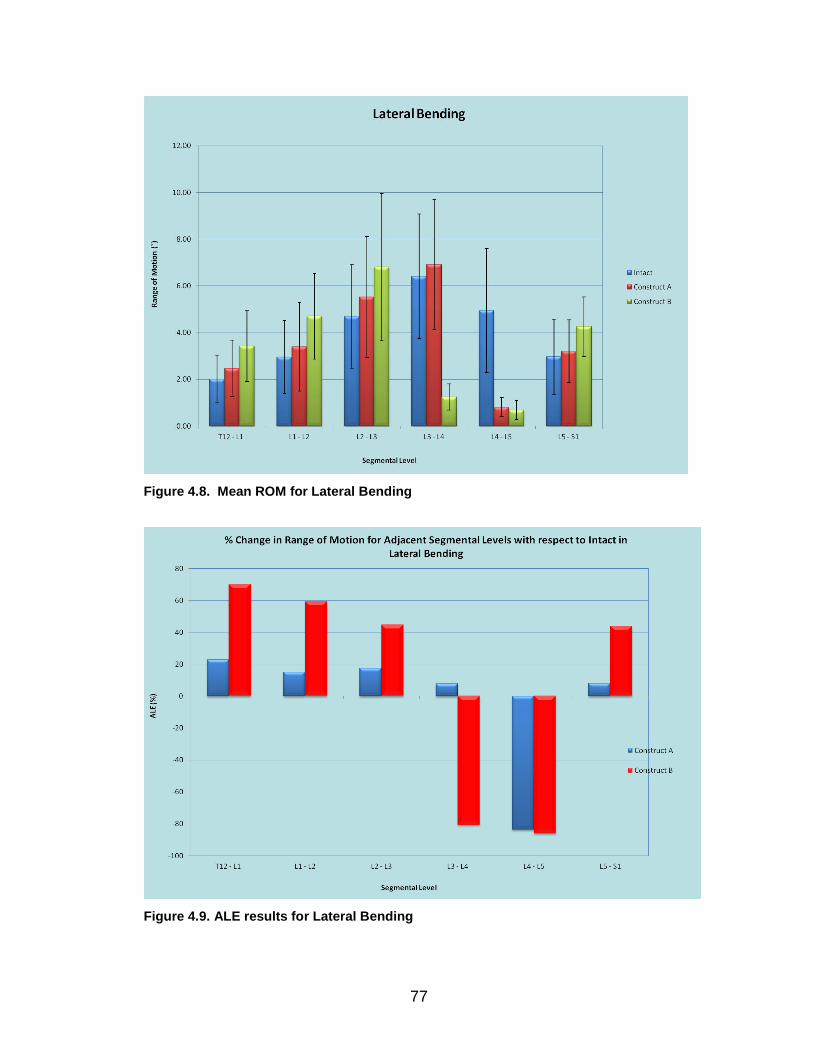
77

Figure 4.8. Mean ROM for Lateral Bending

Figure 4.9. ALE results for Lateral Bending

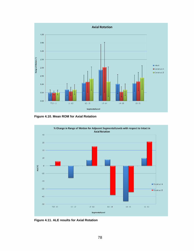
78

Figure 4.10. Mean ROM for Axial Rotation

Figure 4.11. ALE results for Axial Rotation

79

4.10 References

1. Gibson JN, Waddell G: Surgery for degenerative lumbar spondylosis:

Updated Cochrane review. Spine 2005; 30:2312 - 2320

2. Schulte TL, Hurschler C, Haversath M, Liljenqvist U, Bullmann V, Filler

TJ, Osada N, Fallenberg EM, Hackenberg L: The effect of dynamic semi-

rigid implants on the range of motion of lumbar motion segments after

decompression. Eur. Spine J 2008; 17: 1057 - 1065

3. Hilibrand AS, Robbins M : Adjacent segment degeneration and adjacent

segment disease: the consequences of spinal fusion? Spine J 2004; 4

(suppl):190 – 194

4. Eck JC, Humphreys SC, Hodges SD: Adjacent-segment degeneration

after Lumbar fusion: a review of clinical, biomechanical, and radiologic

studies. Am J Orthop , 1999. 28(6):336 – 340.

5. Lee CK: Accelerated degeneration of the segment adjacent to a lumbar

fusion. Spine 1988; 13(3):375 -377

6. Ghiselli JN, Wang JC, Bhatia NN, Hsu WK, Dawson EG: Adjacent

segment degeneration in the lumbar spine. J bone join Surgery Am 2004;

86: 1497 – 1503.

7. Schlegel JD, Smith JA, Schleusener RL: Lumbar motion segment

pathology adjacent to thoracolumbar, lumbar, and lumbosacral fusions.

Spine 1996; 21: 970 – 981.

8. Panjabi MM: Hybrid multidirectional test method to evaluate spinal

adjacent-level effects. Clin Biomech. 2007 Mar;22(3):257-65.

80

9. Panjabi MM, Henderson G, James Y, Timm JP: StabilimaxNZ) versus

simulated fusion: evaluation of adjacent-level effects. Eur Spine J. 2007

Dec;16 (12):2159-65.

10. Panjabi MM, Henderson G, Abjornson C, Yue J: Multidirectional testing of

one- and two-level ProDisc-L versus simulated fusions. Spine 2007;

32(12):1311-9.

11. Panjabi MM, Malcolmson G, Teng E, Tominaga Y, Henderson G, Serhan

H: Hybrid testing of lumbar CHARITE discs versus fusions. Spine 2007;

32(9):959-966

12. Goel VK, Grauer JN, Patel TCh, Biyani A, Sairyo K, Vishnubhotla

S, Matyas A, Cowgill I, Shaw M, Long R, Dick D, Panjabi MM, Serhan H:

Effects of charité artificial disc on the implanted and adjacent spinal

segments mechanics using a hybrid testing protocol. Spine 2005; 30

(24):2755-2764.

13. Schilling C, Krüger S, Grupp TM, Duda GN, Blömer W, Rohlmann A: The

effect of design parameters of dynamic pedicle screw systems on

kinematics and load bearing: an in vitro study. Eur. Spine J 2011; 20: 297

– 307.

14. Kim SH, Chang UK, Chang JC, Chun KS, Lim TJ, Kim DH: The Changes

in Range of Motion after a Lumbar Spinal Arthroplasty with Charité in the

Human Cadaveric Spine under Physiologic Compressive Follower

Preload: A Comparative Study between Load Control Protocol and Hybrid

Protocol. J Korean Neurosurg Soc. 2009 Aug;46 (2):144-51.

81

15. Kim CH, Chung CK, Jahng TA: Comparisons of outcomes after single or

multilevel dynamic stabilization: effects on adjacent segment. J Spinal

Disord Tech 2011; 24(1): 60 – 67.

16. Cakir B, Carazzo C, Schmidt R, Mattes T, Reichel H, Käfer W: Adjacent

segment mobility after rigid and semi rigid instrumentation of the lumbar

spine. Spine 2009; 34: 1287 – 1291.

17. Kumar A, Beastall J, Hughes J, Karadimas EJ, Nicol M, Smith F, Wardlaw

D: Disc changes in the bridged and adjacent segments after Dynesys

dynamic stabilization system after two years. Spine 2008; 33:2909-2914

18. Yamamoto I, Panjabi MM, Crisco T, Oxland T. Three-dimensional

movements of the whole lumbar spine and lumbosacral joint.

Spine 1989. 14(11):1256-60

19. Panjabi M, Dvorak J, Crisco JJ 3rd, Oda T, Wang P, Grob D. Effects of

alar ligament transection on upper cervical spine rotation. J Orthop

Res. 1991 Jul;9(4):584-93.

20. Goel VK, Clark CR, Gallaes K, Liu YK. Moment-rotation relationships of

the ligamentous occipito-atlanto-axial complex. J Biomech. , 1988;

21(8):673-80.

21. Niosi CA, Zhu QA, Wilson DC, Keynan O, Wilson DR, Oxland TR:

Biomechanical characterization of the three-dimensional kinematic

behaviour of the Dynesys dynamic stabilization system: an in vitro study.

Eur. Spine J 2006; 15: 913 – 922.

82

22. Gedet P, Haschtmann D, Thistlethwaite PA, Ferguson SJ: Comparative

biomechanical investigation of a modular dynamic lumbar stabilization

system and the Dynesys system. Eur Spine 2009; 18: 1504 – 1511

23. Schmoelz W, Huber JF, Nydegger T, Dipl-Ing, Claes L, Wilke HJ.:

Dynamic stabilization of the lumbar spine and its effect on adjacent

segments: an in vitro experiment. J Spinal Disord Tech 2003; 16: 418 –

423.

24. Cheng BC, Gordon J, Cheng J, Welch WC: Immediate Biomechanical

Effects of Lumbar Posterior Dynamic Stabilization Above a Circumferential

Fusion. Spine 2007. 32(23):2551-57

83

CHAPTER V

INTRODUCTION

The previous chapters explained in detail in vitro biomechanical testing

and its implementation in evaluating spinal implants. Two different spinal

implants were evaluated and their effect on the spine was analyzed. This chapter

explains in detail the development of a finite element model and its validation

using the in vitro test data.

5.1 Role of Finite Element Models of the Spine

Finite element modeling is a numerical method used for analyzing

complex structures. The application of finite element modeling in spine has been

primarily used to study the behavior of the spine under varying boundary and

loading conditions. Advancements in numerical techniques, medical imaging and

computer technology facilitate the acquisition of detailed quantitative geometric

information of anatomical structures – which in turn facilitates both research and

patient care. Patient-specific models can be developed quickly to aid clinicians in

their decision making process regarding the management of spinal ailments.

These models can be used to simulate and evaluate various clinical scenarios

such as the extent of degeneration, the biomechanical efficacy of surgical

84

procedures (e.g. laminectomy and fusion), and the placement of implants for

stabilization, etc.

A finite element model of the spine has the advantage of not only

providing useful information about a model’s response to an external load, but it

also has the ability to predict and approximate the internal stresses/strains that

occur within the modeled structure 3-4. Finite element spine models can be used

for conducting comparative analysis of spinal implants through the evaluation of

their respective effects on the stability of the spine. In essence, a spine model

can serve as a valuable cost effective tool for the modification of existing or the

design of new spinal implants. Spinal stability following the placement of various

implants can be simulated and analyzed, providing the clinician with valuable

insight into the potential performance of specific implants, before the actual

surgery. These analytical models can provide the flexibility of precisely controlling

a variety of parameters and then studying the effects of these changes on the

behavior of the modeled structure.

Current physical testing methods (both in vivo and in vitro) of the spine,

are fraught with flaws. Such techniques include the testing of animal or human

cadaveric specimens in a mechanical testing machine. Such testing strategies

are expensive and very time consumptive. In addition, in vivo studies are

associated with ethical concerns, the accuracy of data and the interpretation

/correlation of results to the human situation1-2. In both in vivio and in vitro

studies, difficulty exists regarding the determination of the internal stresses and

strains within segments. Normal healthy human spines are not readily available

85

for in vitro testing. Loads and muscle forces that are active in normal spine

motion cannot be effectively replicated and the internal stress/strain distribution

within specific tissue components cannot be accurately measured during such

studies. These and more factors create a substantial impetus for improving

existing testing methods through virtual modeling and the further development of

sophisticated three dimensional (3D) finite element models of the spine.

In recent years, there has also been a constant push to try to accomplish

surgical procedures through minimally invasive surgery (MIS) due to their

demonstrated benefits (like less blood loss and earlier hospital discharge) when

compared to the traditional open procedures. The increased use and improved

application of MIS techniques is driven by the interests of health care

professionals, industry and patients. The impetus for improvement in MIS

procedures has led to an increase in the development of spinal stabilization

devices that require less invasive surgical exposure for their implantation. Such a

device is the interspinous fixation device (ISD) used to clamp adjacent spinous

elements in rigid alignment in anticipation of spinal fusion. The clinical

indications for the use of non-fusion interspinous fixation devices are for lumbar

spinal stenosis and painful facet arthrosis. With the clinical success of those

devices a number of interspinous fixation devices have been tested or introduced

into clinical use.

The use of ISDs to promote interspinous fusion is not a new idea. Similar

implants have been used in the past, but their use has been discontinued when

faced with greater stability and better clinical results of more modern

86

instrumentation implants. The Aspen ISD, produced by Lanx (Broomfield, CO) is

representative of implants seeking to augment interbody fusion techniques while

reducing the need for transpedicular fixation. The aim of the implant is to

increase segmental stability with the purpose of improving the fusion rate; the

advantage being a minimally invasive surgery. The insertion of the implant

requires only a small midline incision with no additional lateral exposure. The

device is placed between the spinous processes of an unstable segment with

only the disruption of the interspinous ligament during implantation while the

supraspinous ligament remains intact.

The purpose of this study was to develop a finite element model of a

lumbar spinal segment and evaluate the effect of placing the new interspinous

fixation device with an interbody spacer model on kinematics of the lumbar spine

motion. The finite element model was used to compare the device's ability to

stabilize the motion of a lumbar segment in flexion-extension, lateral bending,

and axial rotation. The ISD was modeled as a stand-alone device, and in

combination with a unilateral pedicle screw fixation, relative to a more traditional

fixation construct using bilateral pedicle screw fixation, which is considered the

current gold standard of rigid fixation.

5.2 Methods

A three-dimensional finite element model was developed using CT images

obtained from an intact L3-L4 cadaveric spinal motion segment. The CT images

had a resolution of 0.75 mm.

87

5.2.1 Vertebral bodies. The CT image processing to develop a three-

dimensional model of the vertebrae was done using the commercially available

software, MIMICS 9.0 (Materialise, MI, USA). A series of image segmentation

and region-growing operations were carried out on the CT images. These

operations were done to isolate the bony tissue from the soft tissue and to extract

the desired geometrical information of the spinal motion segment. The

segmented CT images were then converted to a three dimensional surface

model using a set of interpolation and smoothening functions available in

MIMICS. The STL+ module found within MIMICS was then used to convert the

model into a triangular surface mesh. The FE module also found in MIMICS was

used to improve the quality of the triangular mesh through a series of

optimization algorithms. The optimized surface mesh model made up of

triangular elements was converted to a solid mesh model made of tetrahedral

elements. The solid model was then exported into a commercially available finite

element program, ABAQUS (Simulia Corporation, RI, USA). A flow chart of all

the operations required to develop a finite element model is shown in Figure 1. In

ABAQUS, the all the exterior elements of the vertebrae were modeled as cortical

bone while all the interior elements were modeled as cancellous bone. Isotropic

material properties were assigned to the elements. (Table 1). Offset elements

were created from the element faces of the facet joints and assigned

cartilaginous properties. In Abaqus, a hard contact surface to surface algorithm

was implemented between the facets with a frictionless tangential contact

property.

88

5.2.2 Intervertebral disc. The poor soft tissue image quality in CT

prevented the development of a surface model of the disc using MIMICS. The

intervertebral disc model was developed using a CAD program, Pro Engineer

(Pro Engineer, Wildfire III, USA). The three-dimensional vertebral bodies

developed in MIMICS were imported into the CAD program and a set of sagittal

planes were created. The cross sections of the vertebral bodies were then traced

onto the planes as shown in Figure 2. Using these sections, curves were then

sketched to fit the upper and lower sections of the endplates. Surfaces were then

fitted onto these sketches and a solid model was extruded from the upper

surface to the lower surface. The solid model was then exported as an Elysium

file into ABAQUS for further preprocessing operations such as partitioning,

element-embedding and meshing. The nucleus pulposus (NP) was modeled

using solid hexahedral elements while the annulus fibrosus (AF) was modeled

using solid hexahedral elements to represent the ground substance with

embedded rebar layers representing collagen fibers.5-7 Four concentric rings of

rebar layers were created in ABAQUS and each ring contained two evenly

spaced rebars (tension-only fibers) oriented at ±30о to the horizontal.5 (Figure 3).

The fiber thickness and stiffness were assigned to increase in the radial direction.

Both nucleus pulposus and the annulus fibrosus were assigned isotropic material

properties. (Table 1). All the superior and inferior elements of the disc were tied

to the vertebral model endplates in ABAQUS.

5.2.3 Ligaments. The spinal motion segment is made up of a number of

ligaments serving as connective tissues between the vertebral bodies. These

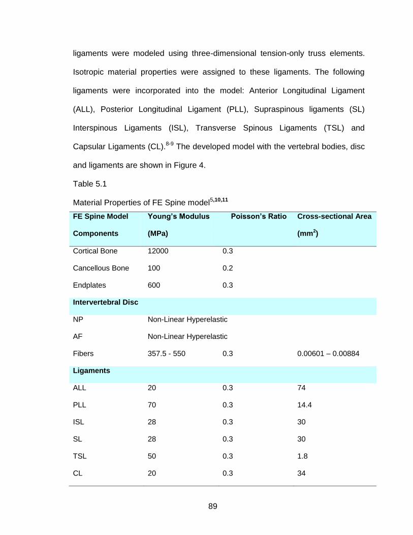
89

ligaments were modeled using three-dimensional tension-only truss elements.

Isotropic material properties were assigned to these ligaments. The following

ligaments were incorporated into the model: Anterior Longitudinal Ligament

(ALL), Posterior Longitudinal Ligament (PLL), Supraspinous ligaments (SL)

Interspinous Ligaments (ISL), Transverse Spinous Ligaments (TSL) and

Capsular Ligaments (CL).8-9 The developed model with the vertebral bodies, disc

and ligaments are shown in Figure 4.

Table 5.1

Material Properties of FE Spine model5,10,11

FE Spine Model

Components

Young’s Modulus

(MPa)

Poisson’s Ratio Cross-sectional Area

(mm2)

Cortical Bone 12000 0.3

Cancellous Bone 100 0.2

Endplates 600 0.3

Intervertebral Disc

NP Non-Linear Hyperelastic

AF Non-Linear Hyperelastic

Fibers 357.5 - 550 0.3 0.00601 – 0.00884

Ligaments

ALL 20 0.3 74

PLL 70 0.3 14.4

ISL 28 0.3 30

SL 28 0.3 30

TSL 50 0.3 1.8

CL 20 0.3 34

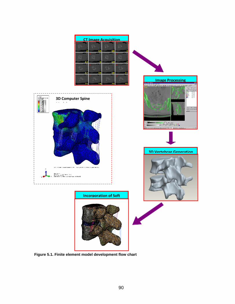
90

CT Image Acquisition

Image Processing

3D Vertebrae Generation

Incorporation of Soft Tissue

3D Computer Spine Model

Figure 5.1. Finite element model development flow chart

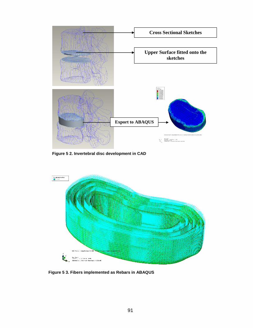
91

Cross Sectional Sketches

Upper Surface fitted onto the

sketches

Export to ABAQUS

Figure 5 2. Invertebral disc development in CAD

Figure 5 3. Fibers implemented as Rebars in ABAQUS

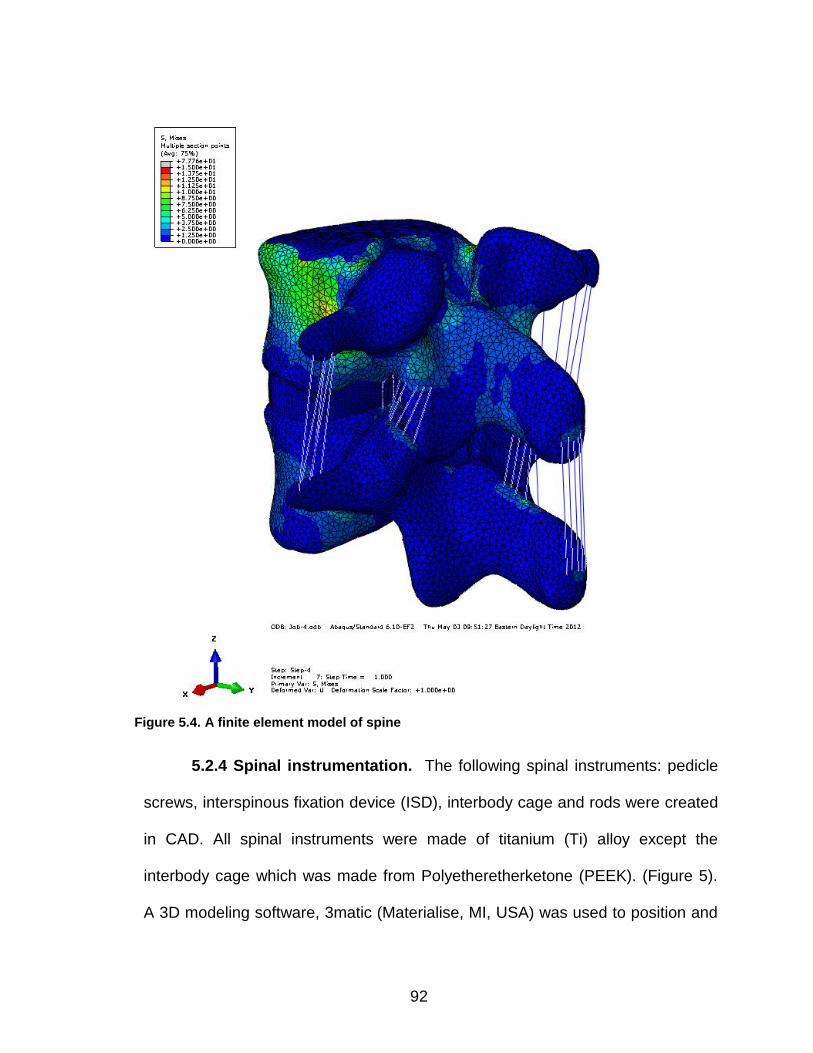
92

5.2.4 Spinal instrumentation. The following spinal instruments: pedicle

screws, interspinous fixation device (ISD), interbody cage and rods were created

in CAD. All spinal instruments were made of titanium (Ti) alloy except the

interbody cage which was made from Polyetheretherketone (PEEK). (Figure 5).

A 3D modeling software, 3matic (Materialise, MI, USA) was used to position and

Figure 5.4. A finite element model of spine

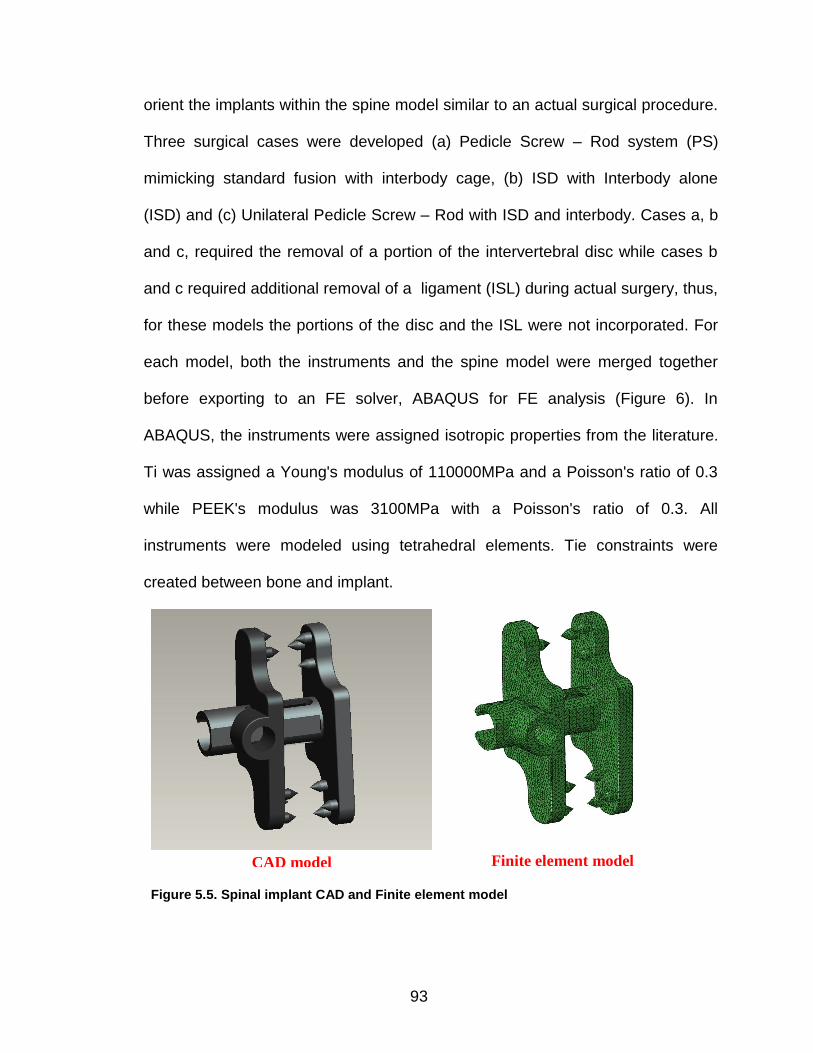
93

orient the implants within the spine model similar to an actual surgical procedure.

Three surgical cases were developed (a) Pedicle Screw – Rod system (PS)

mimicking standard fusion with interbody cage, (b) ISD with Interbody alone

(ISD) and (c) Unilateral Pedicle Screw – Rod with ISD and interbody. Cases a, b

and c, required the removal of a portion of the intervertebral disc while cases b

and c required additional removal of a ligament (ISL) during actual surgery, thus,

for these models the portions of the disc and the ISL were not incorporated. For

each model, both the instruments and the spine model were merged together

before exporting to an FE solver, ABAQUS for FE analysis (Figure 6). In

ABAQUS, the instruments were assigned isotropic properties from the literature.

Ti was assigned a Young's modulus of 110000MPa and a Poisson's ratio of 0.3

while PEEK's modulus was 3100MPa with a Poisson's ratio of 0.3. All

instruments were modeled using tetrahedral elements. Tie constraints were

created between bone and implant.

CAD model Finite element model

Figure 5.5. Spinal implant CAD and Finite element model

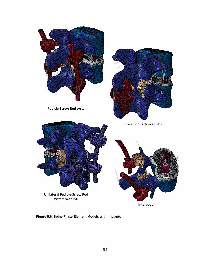
94

Pedicle-Screw Rod system

Interspinous device (ISD)

Unilateral Pedicle-Screw Rod system with ISD

Interbody

Figure 5.6. Spine Finite Element Models with implants

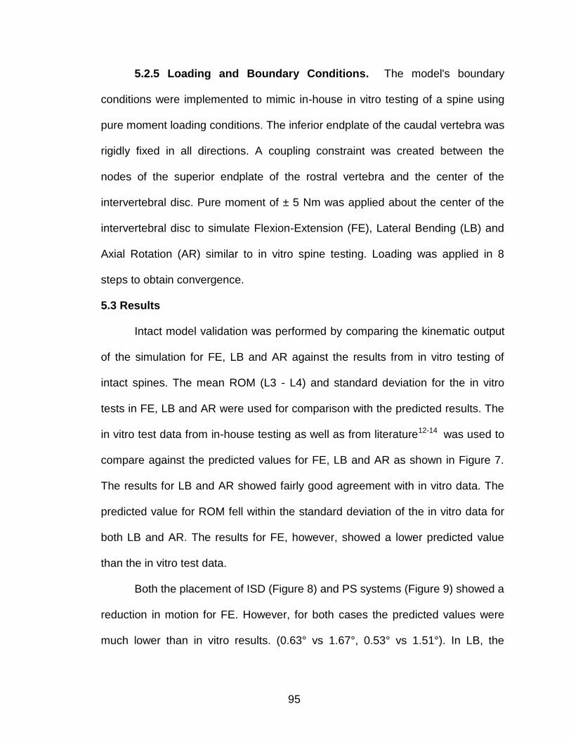
95

5.2.5 Loading and Boundary Conditions. The model's boundary

conditions were implemented to mimic in-house in vitro testing of a spine using

pure moment loading conditions. The inferior endplate of the caudal vertebra was

rigidly fixed in all directions. A coupling constraint was created between the

nodes of the superior endplate of the rostral vertebra and the center of the

intervertebral disc. Pure moment of ± 5 Nm was applied about the center of the

intervertebral disc to simulate Flexion-Extension (FE), Lateral Bending (LB) and

Axial Rotation (AR) similar to in vitro spine testing. Loading was applied in 8

steps to obtain convergence.

5.3 Results

Intact model validation was performed by comparing the kinematic output

of the simulation for FE, LB and AR against the results from in vitro testing of

intact spines. The mean ROM (L3 - L4) and standard deviation for the in vitro

tests in FE, LB and AR were used for comparison with the predicted results. The

in vitro test data from in-house testing as well as from literature12-14 was used to

compare against the predicted values for FE, LB and AR as shown in Figure 7.

The results for LB and AR showed fairly good agreement with in vitro data. The

predicted value for ROM fell within the standard deviation of the in vitro data for

both LB and AR. The results for FE, however, showed a lower predicted value

than the in vitro test data.

Both the placement of ISD (Figure 8) and PS systems (Figure 9) showed a

reduction in motion for FE. However, for both cases the predicted values were

much lower than in vitro results. (0.63° vs 1.67°, 0.53° vs 1.51°). In LB, the

96

results showed that following placement of the PS system (Figure 10), there was

a reduction in motion from 6.9° to 0.73°. Similarly we found that ISD (Figure 11)

reduced motion from 6.9° to 0.99°. In AR, we found that motion decreased to

0.58° from intact state (5.7°) following the placement of ISD (Figure 12) while PS

system (Figure 13) caused a decrease in motion from intact (5.7°) to 0.91°.

Figure 5.7. Intact Spine Model results compared against in vitro data

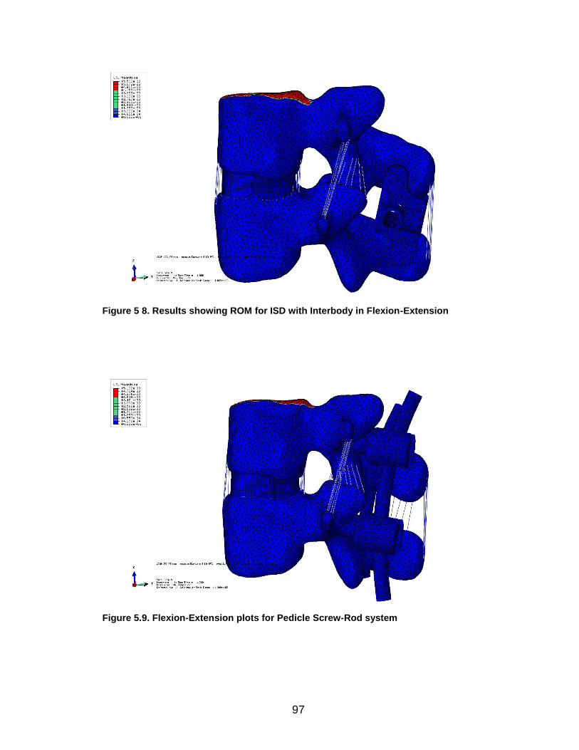
97

Figure 5 8. Results showing ROM for ISD with Interbody in Flexion-Extension

Figure 5.9. Flexion-Extension plots for Pedicle Screw-Rod system

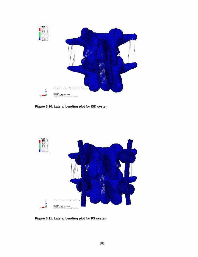
98

Figure 5.10. Lateral bending plot for ISD system

Figure 5.11. Lateral bending plot for PS system

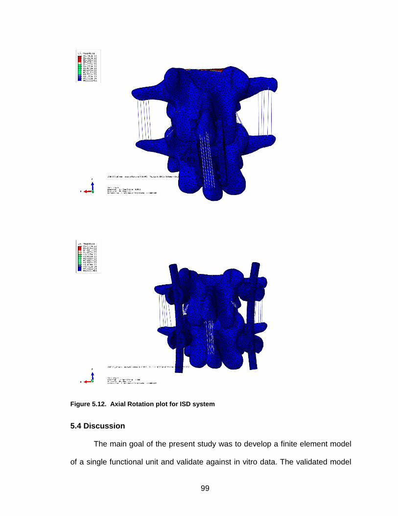
99

Figure 5.12. Axial Rotation plot for ISD system

5.4 Discussion

The main goal of the present study was to develop a finite element model

of a single functional unit and validate against in vitro data. The validated model

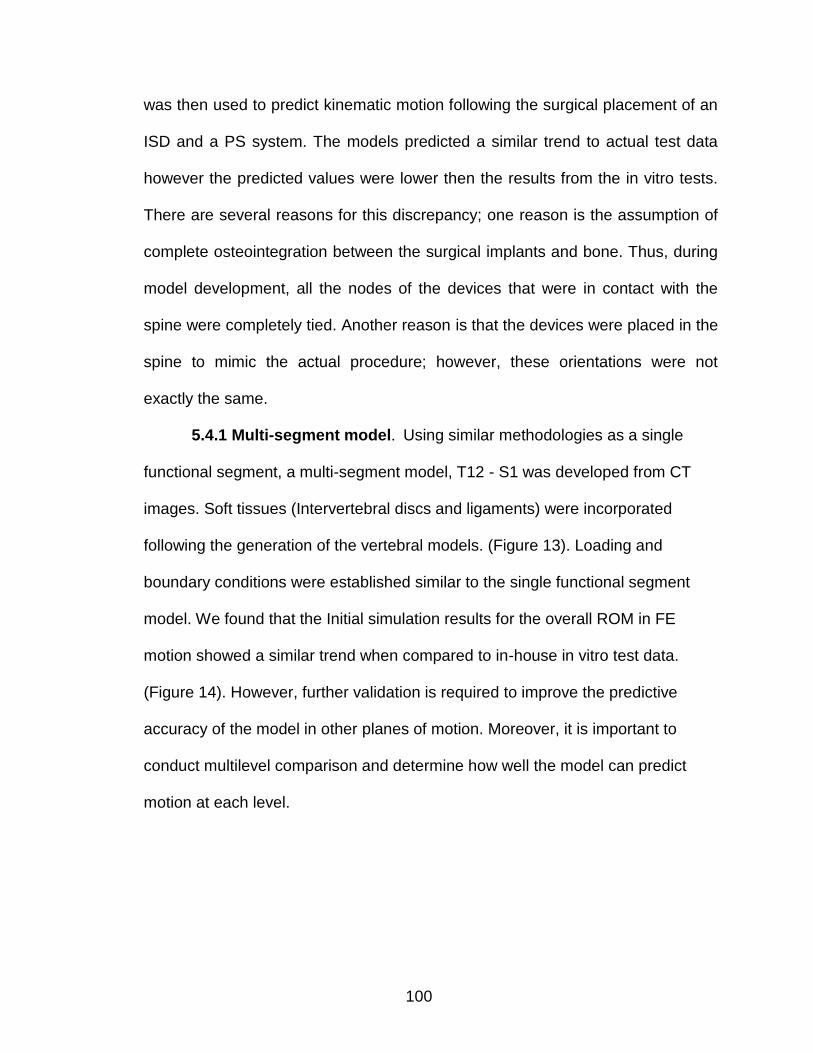
100

was then used to predict kinematic motion following the surgical placement of an

ISD and a PS system. The models predicted a similar trend to actual test data

however the predicted values were lower then the results from the in vitro tests.

There are several reasons for this discrepancy; one reason is the assumption of

complete osteointegration between the surgical implants and bone. Thus, during

model development, all the nodes of the devices that were in contact with the

spine were completely tied. Another reason is that the devices were placed in the

spine to mimic the actual procedure; however, these orientations were not

exactly the same.

5.4.1 Multi-segment model. Using similar methodologies as a single

functional segment, a multi-segment model, T12 - S1 was developed from CT

images. Soft tissues (Intervertebral discs and ligaments) were incorporated

following the generation of the vertebral models. (Figure 13). Loading and

boundary conditions were established similar to the single functional segment

model. We found that the Initial simulation results for the overall ROM in FE

motion showed a similar trend when compared to in-house in vitro test data.

(Figure 14). However, further validation is required to improve the predictive

accuracy of the model in other planes of motion. Moreover, it is important to

conduct multilevel comparison and determine how well the model can predict

motion at each level.

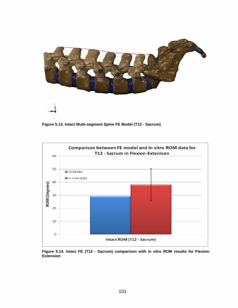
101

Figure 5.13. Intact Multi-segment Spine FE Model (T12 - Sacrum)

Figure 5.14. Intact FE (T12 - Sacrum) comparison with in vitro ROM results for Flexion-Extension

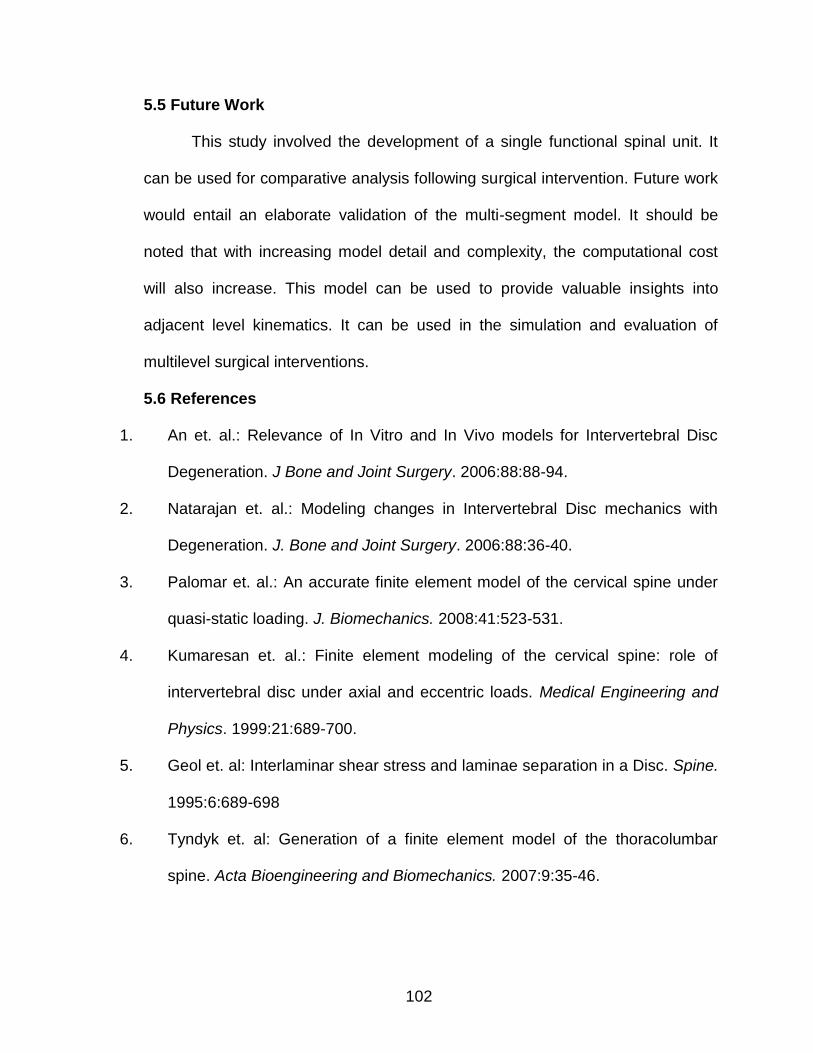
102

5.5 Future Work

This study involved the development of a single functional spinal unit. It

can be used for comparative analysis following surgical intervention. Future work

would entail an elaborate validation of the multi-segment model. It should be

noted that with increasing model detail and complexity, the computational cost

will also increase. This model can be used to provide valuable insights into

adjacent level kinematics. It can be used in the simulation and evaluation of

multilevel surgical interventions.

5.6 References

1. An et. al.: Relevance of In Vitro and In Vivo models for Intervertebral Disc

Degeneration. J Bone and Joint Surgery. 2006:88:88-94.

2. Natarajan et. al.: Modeling changes in Intervertebral Disc mechanics with

Degeneration. J. Bone and Joint Surgery. 2006:88:36-40.

3. Palomar et. al.: An accurate finite element model of the cervical spine under

quasi-static loading. J. Biomechanics. 2008:41:523-531.

4. Kumaresan et. al.: Finite element modeling of the cervical spine: role of

intervertebral disc under axial and eccentric loads. Medical Engineering and

Physics. 1999:21:689-700.

5. Geol et. al: Interlaminar shear stress and laminae separation in a Disc. Spine.

1995:6:689-698

6. Tyndyk et. al: Generation of a finite element model of the thoracolumbar

spine. Acta Bioengineering and Biomechanics. 2007:9:35-46.

103

7. Vadapalli et. al.: Biomechanical rationale for using Polyetheretherketone

(PEEK) spacers for Lumbar Interbody Fusion – A finite element study. Spine.

2006:26: 992-998

8. Teo et. al.: Evaluation of the role of ligaments, facets and disc nucleus in

lower cervical spine under compression and sagittal moments using finite

element method. Medical Engineering and Physics. 2001:23:155-164.

9. Yoganandan et. al.: Finite element modeling of the C4-C6 cervical spine unit.

Medical Engineering and Physics. 1996:18:569-574.

10. Sylvestre P et. al.: Finite Element Modeling of the growth plate in a detailed

spine model. Med bio Eng Comput. 2007: 45: 977 - 988

11. Rohlmann A et. al.: Comparison of the effects of bilateral posterior dynamic

and rigid fixation devices on the loads in the lumbar spine: a finite element

analysis. Eur. Spine J. (2007). 16:1223 - 1231.

12. Panjabi MM, Oxland TR, Yamamoto I, Crisco JJ. Mechanical behavior of the

human lumbar and lumbosacral spine as shown by three-dimensionalload-

displacement curves. J Bone Joint Surg Am. 1994 Mar;76(3):413-24

13. Cholewicki J, Crisco JJ 3rd, Oxland TR, Yamamoto I, Panjabi MM. Effects of

posture and structure on three-dimensional coupled rotations in the lumbar

spine. A biomechanical analysis. Spine (Phila Pa 1976). 1996 Nov

1;21(21):2421-8.

14. Yamamoto I, Panjabi MM, Crisco T, Oxland T. Three-dimensional movements

of the whole lumbar spine and lumbosacral joint. Spine (Phila Pa

1976). 1989 Nov;14(11):1256-60.

104

105

Chapter VI

STUDY CONCLUSIONS

In vitro biomechanical test methodology was successfully developed for

testing spinal constructs. Two unique implants were evaluated and their test

results were presented. The current setup using a robotic system can be

modified to study not only the lumbar spine but other spinal regions such as

cervical and thoracic. The fixtures were custom designed and can match the

different vertebral sizes. The custom force-torque program used in running the

robot can be used to apply known physiological loads on the spine in a

reproducible and accurate manner. The robotic system enables easier

manipulation of both boundary and loading conditions during testing when

compared to older static pure moment systems from the literature.

The finite element model of a single FSU, L3-4, was developed using CT

image data from one of the test specimens used in the in vitro study. The model

was then validated using the in vitro test data of the ISD study. A multi-segment

model, T12- Sacrum was also developed and evaluated using in vitro test data.

106

APPENDICES

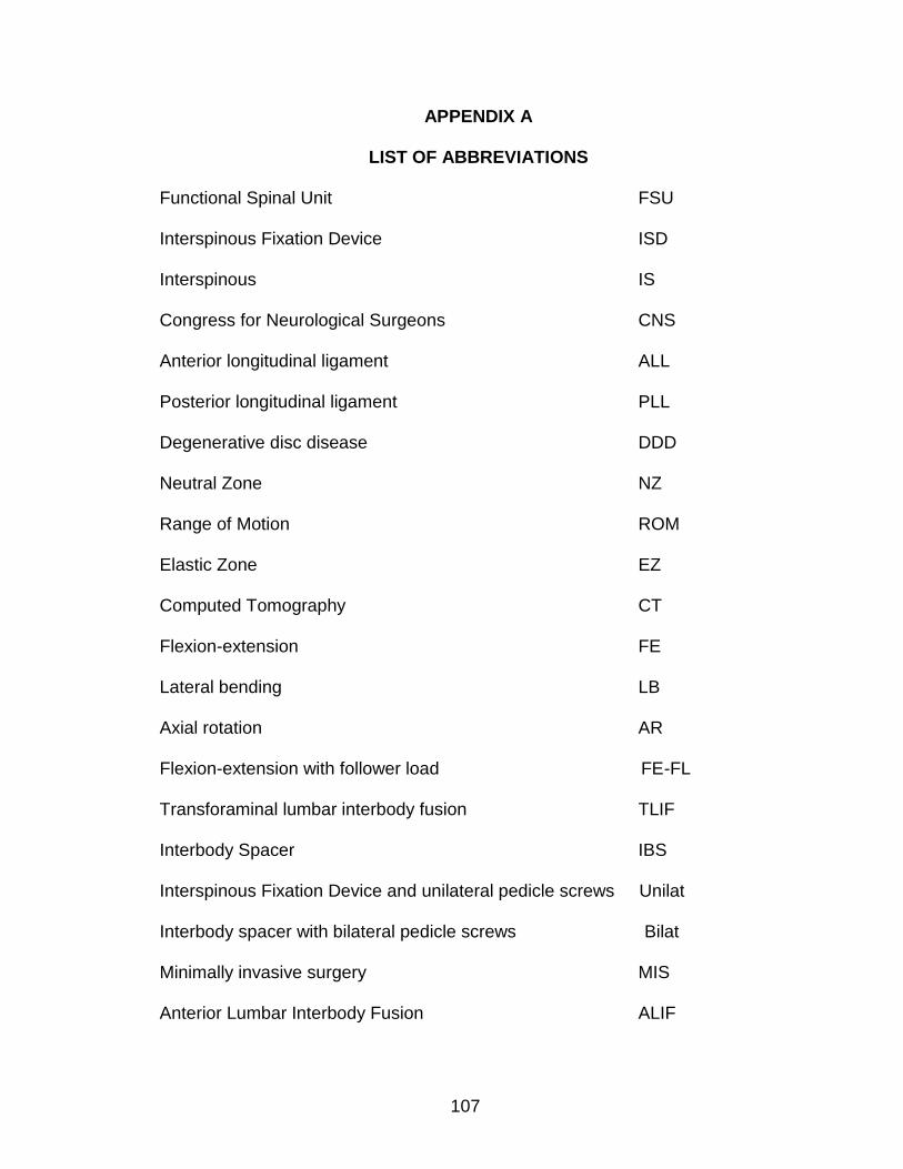
107

APPENDIX A

LIST OF ABBREVIATIONS

Functional Spinal Unit FSU

Interspinous Fixation Device ISD

Interspinous IS

Congress for Neurological Surgeons CNS

Anterior longitudinal ligament ALL

Posterior longitudinal ligament PLL

Degenerative disc disease DDD

Neutral Zone NZ

Range of Motion ROM

Elastic Zone EZ

Computed Tomography CT

Flexion-extension FE

Lateral bending LB

Axial rotation AR

Flexion-extension with follower load FE-FL

Transforaminal lumbar interbody fusion TLIF

Interbody Spacer IBS

Interspinous Fixation Device and unilateral pedicle screws Unilat

Interbody spacer with bilateral pedicle screws Bilat

Minimally invasive surgery MIS

Anterior Lumbar Interbody Fusion ALIF

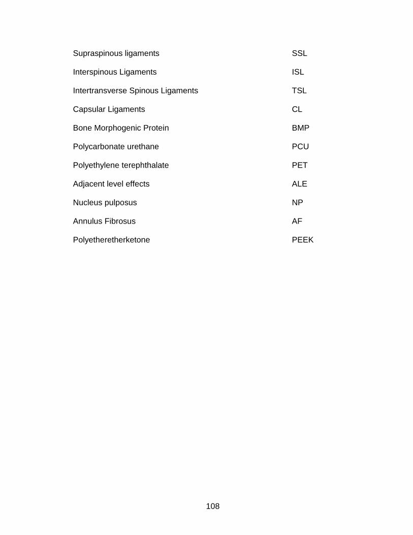
108

Supraspinous ligaments SSL

Interspinous Ligaments ISL

Intertransverse Spinous Ligaments TSL

Capsular Ligaments CL

Bone Morphogenic Protein BMP

Polycarbonate urethane PCU

Polyethylene terephthalate PET

Adjacent level effects ALE

Nucleus pulposus NP

Annulus Fibrosus AF

Polyetheretherketone PEEK

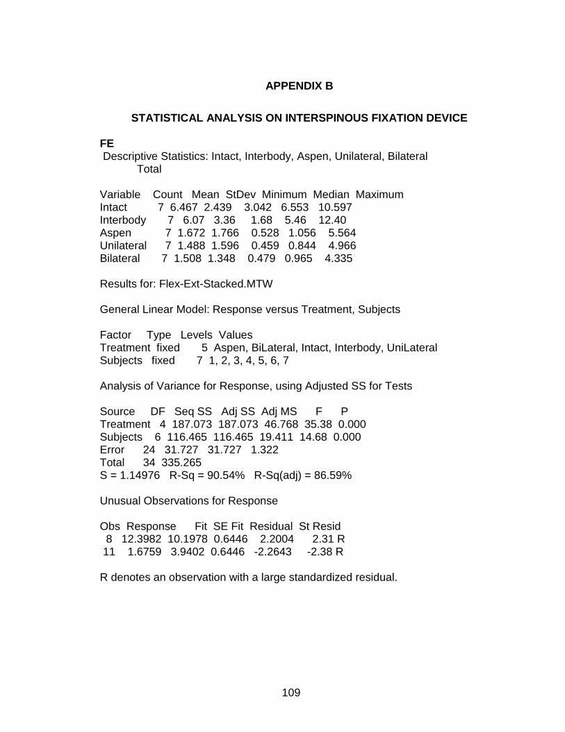
109

APPENDIX B

STATISTICAL ANALYSIS ON INTERSPINOUS FIXATION DEVICE

FE Descriptive Statistics: Intact, Interbody, Aspen, Unilateral, Bilateral Total Variable Count Mean StDev Minimum Median Maximum Intact 7 6.467 2.439 3.042 6.553 10.597 Interbody 7 6.07 3.36 1.68 5.46 12.40 Aspen 7 1.672 1.766 0.528 1.056 5.564 Unilateral 7 1.488 1.596 0.459 0.844 4.966 Bilateral 7 1.508 1.348 0.479 0.965 4.335 Results for: Flex-Ext-Stacked.MTW General Linear Model: Response versus Treatment, Subjects Factor Type Levels Values Treatment fixed 5 Aspen, BiLateral, Intact, Interbody, UniLateral Subjects fixed 7 1, 2, 3, 4, 5, 6, 7 Analysis of Variance for Response, using Adjusted SS for Tests Source DF Seq SS Adj SS Adj MS F P Treatment 4 187.073 187.073 46.768 35.38 0.000 Subjects 6 116.465 116.465 19.411 14.68 0.000 Error 24 31.727 31.727 1.322 Total 34 335.265 S = 1.14976 R-Sq = 90.54% R-Sq(adj) = 86.59% Unusual Observations for Response Obs Response Fit SE Fit Residual St Resid 8 12.3982 10.1978 0.6446 2.2004 2.31 R 11 1.6759 3.9402 0.6446 -2.2643 -2.38 R R denotes an observation with a large standardized residual.

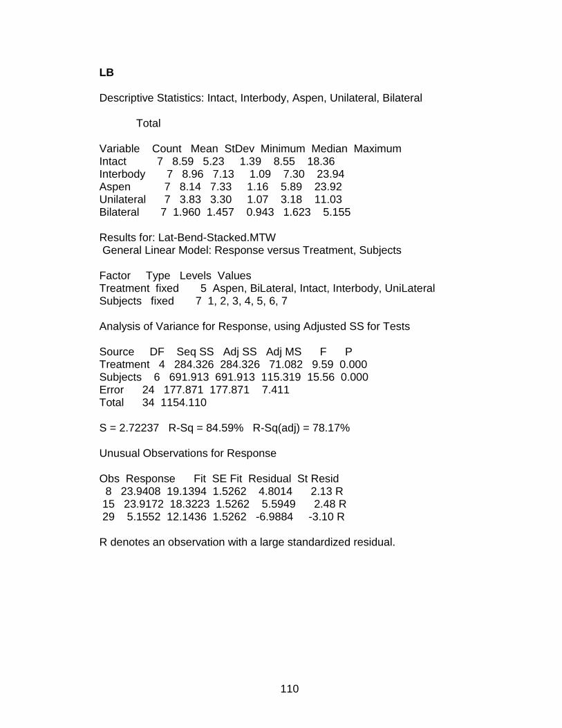
110

LB Descriptive Statistics: Intact, Interbody, Aspen, Unilateral, Bilateral Total Variable Count Mean StDev Minimum Median Maximum Intact 7 8.59 5.23 1.39 8.55 18.36 Interbody 7 8.96 7.13 1.09 7.30 23.94 Aspen 7 8.14 7.33 1.16 5.89 23.92 Unilateral 7 3.83 3.30 1.07 3.18 11.03 Bilateral 7 1.960 1.457 0.943 1.623 5.155 Results for: Lat-Bend-Stacked.MTW General Linear Model: Response versus Treatment, Subjects Factor Type Levels Values Treatment fixed 5 Aspen, BiLateral, Intact, Interbody, UniLateral Subjects fixed 7 1, 2, 3, 4, 5, 6, 7 Analysis of Variance for Response, using Adjusted SS for Tests Source DF Seq SS Adj SS Adj MS F P Treatment 4 284.326 284.326 71.082 9.59 0.000 Subjects 6 691.913 691.913 115.319 15.56 0.000 Error 24 177.871 177.871 7.411 Total 34 1154.110 S = 2.72237 R-Sq = 84.59% R-Sq(adj) = 78.17% Unusual Observations for Response Obs Response Fit SE Fit Residual St Resid 8 23.9408 19.1394 1.5262 4.8014 2.13 R 15 23.9172 18.3223 1.5262 5.5949 2.48 R 29 5.1552 12.1436 1.5262 -6.9884 -3.10 R R denotes an observation with a large standardized residual.

111

AR Descriptive Statistics: Intact, Interbody, Aspen, Unilateral, Bilateral Total Variable Count Mean StDev Minimum Median Maximum Intact 7 3.986 2.341 0.699 3.959 7.443 Interbody 7 3.693 2.160 0.892 3.507 6.875 Aspen 7 3.967 2.577 0.781 3.372 7.968 Unilateral 7 2.328 1.330 0.651 2.387 4.653 Bilateral 7 1.394 0.731 0.604 1.406 2.843 Results for: Axial-Rot-Stacked.MTW General Linear Model: Response versus Treatment, Subjects Factor Type Levels Values Treatment fixed 5 Aspen, BiLateral, Intact, Interbody, UniLateral Subjects fixed 7 1, 2, 3, 4, 5, 6, 7 Analysis of Variance for Response, using Adjusted SS for Tests Source DF Seq SS Adj SS Adj MS F P Treatment 4 37.749 37.749 9.437 9.12 0.000 Subjects 6 89.681 89.681 14.947 14.44 0.000 Error 24 24.843 24.843 1.035 Total 34 152.274 S = 1.01742 R-Sq = 83.68% R-Sq(adj) = 76.89% Unusual Observations for Response Obs Response Fit SE Fit Residual St Resid 15 7.96795 6.18949 0.57038 1.77846 2.11 R 30 1.41579 3.46735 0.57038 -2.05156 -2.44 R R denotes an observation with a large standardized residual. Results for: Flex-Ext.MTW Paired T-Test and CI: Aspen, Unilateral Paired T for Aspen - Unilateral

112

N Mean StDev SE Mean Aspen 7 1.672 1.766 0.668 Unilateral 7 1.488 1.596 0.603 Difference 7 0.1839 0.1937 0.0732 95% CI for mean difference: (0.0048, 0.3631) T-Test of mean difference = 0 (vs not = 0): T-Value = 2.51 P-Value = 0.046 Paired T-Test and CI: Aspen, Bilateral Paired T for Aspen - Bilateral N Mean StDev SE Mean Aspen 7 1.672 1.766 0.668 Bilateral 7 1.508 1.348 0.509 Difference 7 0.164 0.490 0.185 95% CI for mean difference: (-0.290, 0.617) T-Test of mean difference = 0 (vs not = 0): T-Value = 0.88 P-Value = 0.411 Paired T-Test and CI: Unilateral, Bilateral Paired T for Unilateral - Bilateral N Mean StDev SE Mean Unilateral 7 1.488 1.596 0.603 Bilateral 7 1.508 1.348 0.509 Difference 7 -0.020 0.319 0.121 95% CI for mean difference: (-0.316, 0.275) T-Test of mean difference = 0 (vs not = 0): T-Value = -0.17 P-Value = 0.873 Results for: Lat-Bend.MTW Paired T-Test and CI: Aspen, Unilateral Paired T for Aspen - Unilateral N Mean StDev SE Mean Aspen 7 8.14 7.33 2.77 Unilateral 7 3.83 3.30 1.25 Difference 7 4.31 4.16 1.57

113

95% CI for mean difference: (0.45, 8.16) T-Test of mean difference = 0 (vs not = 0): T-Value = 2.74 P-Value = 0.034 Paired T-Test and CI: Aspen, Bilateral Paired T for Aspen - Bilateral N Mean StDev SE Mean Aspen 7 8.14 7.33 2.77 Bilateral 7 1.96 1.46 0.55 Difference 7 6.18 5.94 2.24 95% CI for mean difference: (0.69, 11.67) T-Test of mean difference = 0 (vs not = 0): T-Value = 2.75 P-Value = 0.033 Paired T-Test and CI: Unilateral, Bilateral Paired T for Unilateral - Bilateral N Mean StDev SE Mean Unilateral 7 3.83 3.30 1.25 Bilateral 7 1.96 1.46 0.55 Difference 7 1.874 1.849 0.699 95% CI for mean difference: (0.164, 3.583) T-Test of mean difference = 0 (vs not = 0): T-Value = 2.68 P-Value = 0.036 Results for: Axial-Rot.MTW Paired T-Test and CI: Aspen, Unilateral Paired T for Aspen - Unilateral N Mean StDev SE Mean Aspen 7 3.967 2.577 0.974 Unilateral 7 2.328 1.330 0.503 Difference 7 1.639 1.349 0.510 95% CI for mean difference: (0.391, 2.886) T-Test of mean difference = 0 (vs not = 0): T-Value = 3.21 P-Value = 0.018 Paired T-Test and CI: Aspen, Bilateral Paired T for Aspen - Bilateral

114

N Mean StDev SE Mean Aspen 7 3.967 2.577 0.974 Bilateral 7 1.394 0.731 0.276 Difference 7 2.574 1.982 0.749 95% CI for mean difference: (0.741, 4.407) T-Test of mean difference = 0 (vs not = 0): T-Value = 3.44 P-Value = 0.014 Paired T-Test and CI: Unilateral, Bilateral Paired T for Unilateral - Bilateral N Mean StDev SE Mean Unilateral 7 2.328 1.330 0.503 Bilateral 7 1.394 0.731 0.276 Difference 7 0.935 0.661 0.250 95% CI for mean difference: (0.323, 1.546) T-Test of mean difference = 0 (vs not = 0): T-Value = 3.74 P-Value = 0.010 Results for: Flex-Ext.MTW Paired T-Test and CI: Intact, Interbody Paired T for Intact - Interbody N Mean StDev SE Mean Intact 7 6.47 2.44 0.92 Interbody 7 6.07 3.36 1.27 Difference 7 0.401 1.979 0.748 95% CI for mean difference: (-1.430, 2.232) T-Test of mean difference = 0 (vs not = 0): T-Value = 0.54 P-Value = 0.611 Paired T-Test and CI: Intact, Aspen Paired T for Intact - Aspen N Mean StDev SE Mean Intact 7 6.467 2.439 0.922 Aspen 7 1.672 1.766 0.668 Difference 7 4.795 1.703 0.644 95% CI for mean difference: (3.220, 6.369) T-Test of mean difference = 0 (vs not = 0): T-Value = 7.45 P-Value = 0.000

115

Paired T-Test and CI: Intact, Unilateral Paired T for Intact - Unilateral N Mean StDev SE Mean Intact 7 6.467 2.439 0.922 Unilateral 7 1.488 1.596 0.603 Difference 7 4.979 1.746 0.660 95% CI for mean difference: (3.364, 6.593) T-Test of mean difference = 0 (vs not = 0): T-Value = 7.55 P-Value = 0.000 Paired T-Test and CI: Intact, Bilateral Paired T for Intact - Bilateral N Mean StDev SE Mean Intact 7 6.467 2.439 0.922 Bilateral 7 1.508 1.348 0.509 Difference 7 4.959 1.851 0.700 95% CI for mean difference: (3.247, 6.671) T-Test of mean difference = 0 (vs not = 0): T-Value = 7.09 P-Value = 0.000 Results for: Lat-Bend.MTW Paired T-Test and CI: Intact, Interbody Paired T for Intact - Interbody N Mean StDev SE Mean Intact 7 8.59 5.23 1.98 Interbody 7 8.96 7.13 2.70 Difference 7 -0.36 3.13 1.18 95% CI for mean difference: (-3.25, 2.53) T-Test of mean difference = 0 (vs not = 0): T-Value = -0.31 P-Value = 0.770 Paired T-Test and CI: Intact, Aspen Paired T for Intact - Aspen

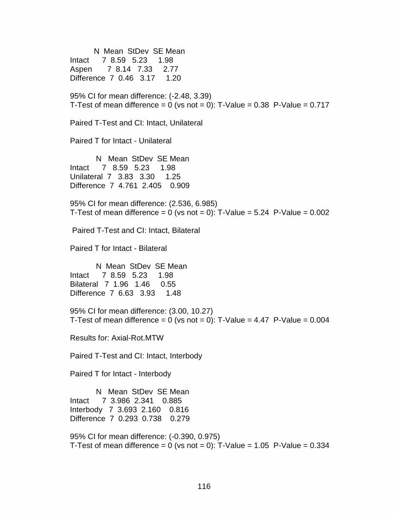
116

N Mean StDev SE Mean Intact 7 8.59 5.23 1.98 Aspen 7 8.14 7.33 2.77 Difference 7 0.46 3.17 1.20 95% CI for mean difference: (-2.48, 3.39) T-Test of mean difference = 0 (vs not = 0): T-Value = 0.38 P-Value = 0.717 Paired T-Test and CI: Intact, Unilateral Paired T for Intact - Unilateral N Mean StDev SE Mean Intact 7 8.59 5.23 1.98 Unilateral 7 3.83 3.30 1.25 Difference 7 4.761 2.405 0.909 95% CI for mean difference: (2.536, 6.985) T-Test of mean difference = 0 (vs not = 0): T-Value = 5.24 P-Value = 0.002 Paired T-Test and CI: Intact, Bilateral Paired T for Intact - Bilateral N Mean StDev SE Mean Intact 7 8.59 5.23 1.98 Bilateral 7 1.96 1.46 0.55 Difference 7 6.63 3.93 1.48 95% CI for mean difference: (3.00, 10.27) T-Test of mean difference = 0 (vs not = 0): T-Value = 4.47 P-Value = 0.004 Results for: Axial-Rot.MTW Paired T-Test and CI: Intact, Interbody Paired T for Intact - Interbody N Mean StDev SE Mean Intact 7 3.986 2.341 0.885 Interbody 7 3.693 2.160 0.816 Difference 7 0.293 0.738 0.279 95% CI for mean difference: (-0.390, 0.975) T-Test of mean difference = 0 (vs not = 0): T-Value = 1.05 P-Value = 0.334

117

Paired T-Test and CI: Intact, Aspen Paired T for Intact - Aspen N Mean StDev SE Mean Intact 7 3.986 2.341 0.885 Aspen 7 3.967 2.577 0.974 Difference 7 0.019 1.527 0.577 95% CI for mean difference: (-1.394, 1.431) T-Test of mean difference = 0 (vs not = 0): T-Value = 0.03 P-Value = 0.975 Paired T-Test and CI: Intact, Unilateral Paired T for Intact - Unilateral N Mean StDev SE Mean Intact 7 3.986 2.341 0.885 Unilateral 7 2.328 1.330 0.503 Difference 7 1.658 1.592 0.602 95% CI for mean difference: (0.185, 3.130) T-Test of mean difference = 0 (vs not = 0): T-Value = 2.75 P-Value = 0.033 Paired T-Test and CI: Intact, Bilateral Paired T for Intact - Bilateral N Mean StDev SE Mean Intact 7 3.986 2.341 0.885 Bilateral 7 1.394 0.731 0.276 Difference 7 2.592 1.988 0.751 95% CI for mean difference: (0.754, 4.431) T-Test of mean difference = 0 (vs not = 0): T-Value = 3.45 P-Value = 0.014

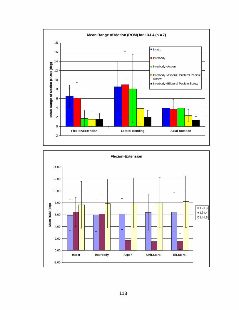
118

Mean Range of Motion (ROM) for L3-L4 (n = 7)

-2

0

2

4

6

8

10

12

14

16

18

Flexion/Extension Lateral Bending Axial Rotation

Me

an

Ra

ng

e o

f M

oti

on

(R

OM

) (d

eg

)Intact

Interbody

Interbody+Aspen

Interbody+Aspen+Unilateral Pedicle

Screw

Interbody+Bilateral Pedicle Screw

Flexion-Extension

-2.00

0.00

2.00

4.00

6.00

8.00

10.00

12.00

14.00

Intact Interbody Aspen UniLateral BiLateral

Mean

RO

M (

deg

)

L2-L3

L3-L4

L4-L5

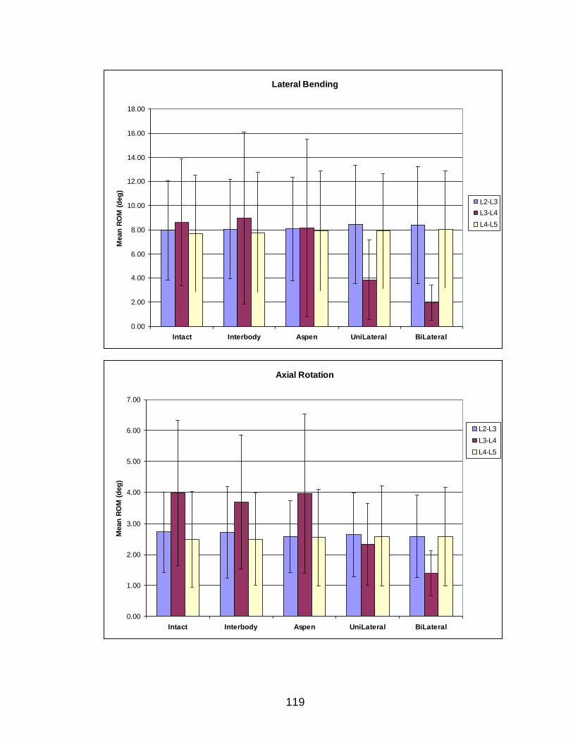
119

Lateral Bending

0.00

2.00

4.00

6.00

8.00

10.00

12.00

14.00

16.00

18.00

Intact Interbody Aspen UniLateral BiLateral

Mean

RO

M (

deg

)

L2-L3

L3-L4

L4-L5

Axial Rotation

0.00

1.00

2.00

3.00

4.00

5.00

6.00

7.00

Intact Interbody Aspen UniLateral BiLateral

Mean

RO

M (

deg

)

L2-L3

L3-L4

L4-L5

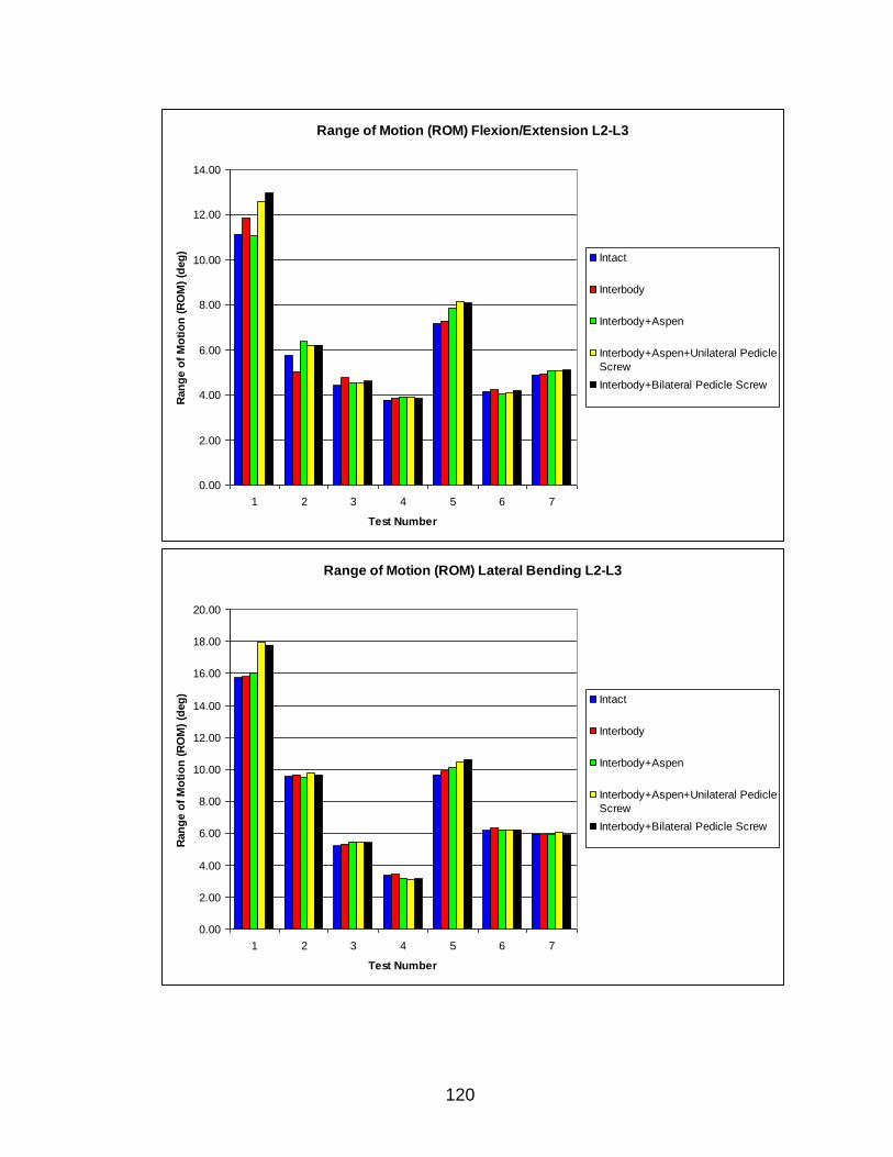
120

Range of Motion (ROM) Flexion/Extension L2-L3

0.00

2.00

4.00

6.00

8.00

10.00

12.00

14.00

1 2 3 4 5 6 7

Test Number

Ran

ge o

f M

oti

on

(R

OM

) (d

eg

)

Intact

Interbody

Interbody+Aspen

Interbody+Aspen+Unilateral Pedicle

Screw

Interbody+Bilateral Pedicle Screw

Range of Motion (ROM) Lateral Bending L2-L3

0.00

2.00

4.00

6.00

8.00

10.00

12.00

14.00

16.00

18.00

20.00

1 2 3 4 5 6 7

Test Number

Ran

ge o

f M

oti

on

(R

OM

) (d

eg

)

Intact

Interbody

Interbody+Aspen

Interbody+Aspen+Unilateral Pedicle

Screw

Interbody+Bilateral Pedicle Screw

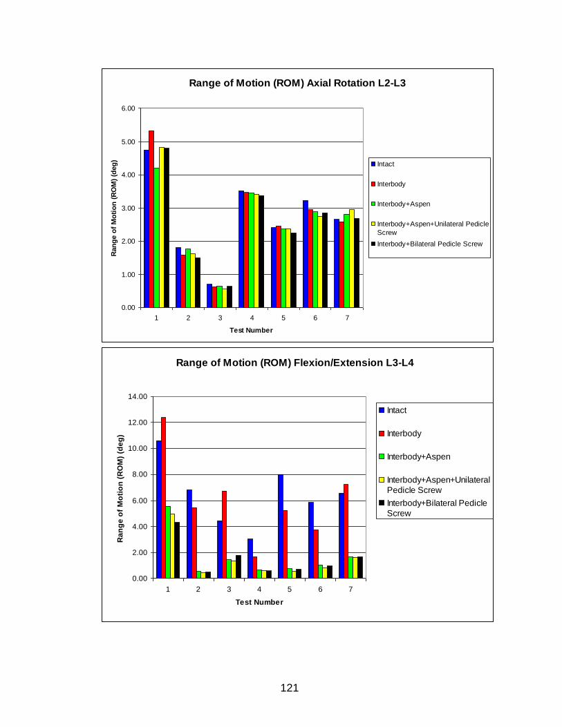
121

Range of Motion (ROM) Axial Rotation L2-L3

0.00

1.00

2.00

3.00

4.00

5.00

6.00

1 2 3 4 5 6 7

Test Number

Ran

ge o

f M

oti

on

(R

OM

) (d

eg

)

Intact

Interbody

Interbody+Aspen

Interbody+Aspen+Unilateral Pedicle

Screw

Interbody+Bilateral Pedicle Screw

Range of Motion (ROM) Flexion/Extension L3-L4

0.00

2.00

4.00

6.00

8.00

10.00

12.00

14.00

1 2 3 4 5 6 7

Test Number

Ra

ng

e o

f M

oti

on

(R

OM

) (d

eg

)

Intact

Interbody

Interbody+Aspen

Interbody+Aspen+Unilateral

Pedicle Screw

Interbody+Bilateral Pedicle

Screw

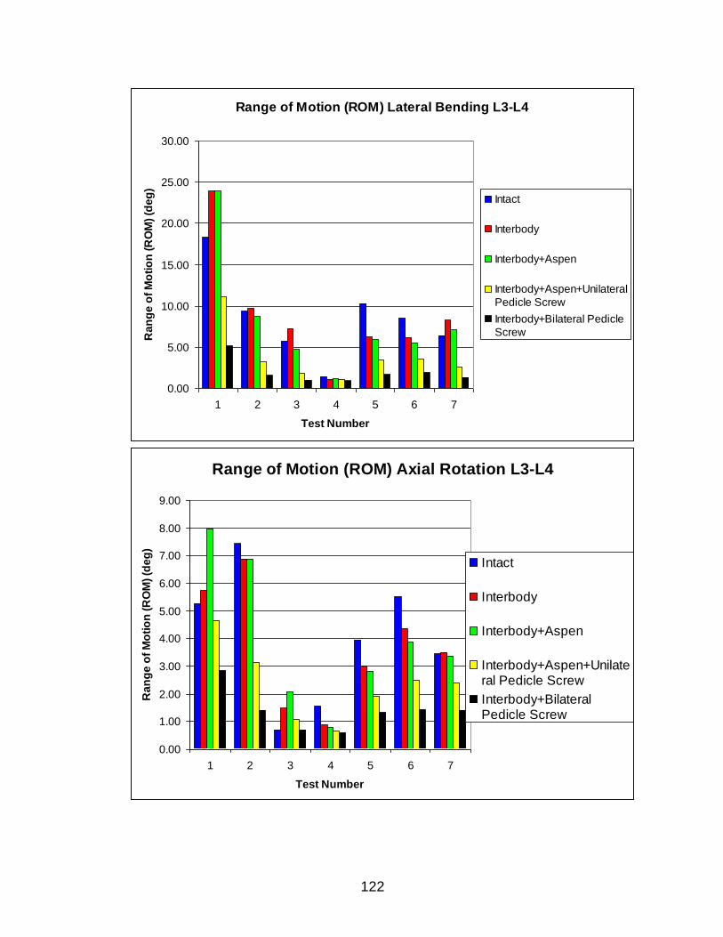
122

Range of Motion (ROM) Lateral Bending L3-L4

0.00

5.00

10.00

15.00

20.00

25.00

30.00

1 2 3 4 5 6 7

Test Number

Ra

ng

e o

f M

oti

on

(R

OM

) (d

eg

)

Intact

Interbody

Interbody+Aspen

Interbody+Aspen+Unilateral

Pedicle Screw

Interbody+Bilateral Pedicle

Screw

Range of Motion (ROM) Axial Rotation L3-L4

0.00

1.00

2.00

3.00

4.00

5.00

6.00

7.00

8.00

9.00

1 2 3 4 5 6 7

Test Number

Ra

ng

e o

f M

oti

on

(R

OM

) (d

eg

)

Intact

Interbody

Interbody+Aspen

Interbody+Aspen+Unilateral Pedicle Screw

Interbody+BilateralPedicle Screw

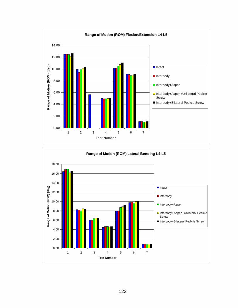
123

Range of Motion (ROM) Flexion/Extension L4-L5

0.00

2.00

4.00

6.00

8.00

10.00

12.00

14.00

1 2 3 4 5 6 7

Test Number

Ra

ng

e o

f M

oti

on

(R

OM

) (d

eg

)

Intact

Interbody

Interbody+Aspen

Interbody+Aspen+Unilateral Pedicle

Screw

Interbody+Bilateral Pedicle Screw

Range of Motion (ROM) Lateral Bending L4-L5

0.00

2.00

4.00

6.00

8.00

10.00

12.00

14.00

16.00

18.00

1 2 3 4 5 6 7

Test Number

Ran

ge o

f M

oti

on

(R

OM

) (d

eg

)

Intact

Interbody

Interbody+Aspen

Interbody+Aspen+Unilateral Pedicle

Screw

Interbody+Bilateral Pedicle Screw

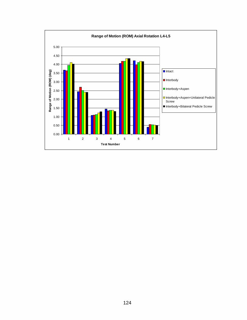
124

Range of Motion (ROM) Axial Rotation L4-L5

0.00

0.50

1.00

1.50

2.00

2.50

3.00

3.50

4.00

4.50

5.00

1 2 3 4 5 6 7

Test Number

Ran

ge o

f M

oti

on

(R

OM

) (d

eg

)

Intact

Interbody

Interbody+Aspen

Interbody+Aspen+Unilateral Pedicle

Screw

Interbody+Bilateral Pedicle Screw

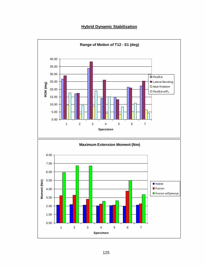
125

Maximum Extension Moment (Nm)

0.00

1.00

2.00

3.00

4.00

5.00

6.00

7.00

8.00

1 2 3 4 5 6 7

Specimen

Mo

men

t (N

m)

Native

Fusion

Fusion w/Dynesys

Hybrid Dynamic Stabilization

Range of Motion of T12 - S1 (deg)

0.00

5.00

10.00

15.00

20.00

25.00

30.00

35.00

40.00

1 2 3 4 5 6 7

Specimen

RO

M (

deg

)

Flex/Ext

Lateral Bending

Axial Rotation

Flex/Ext w/FL

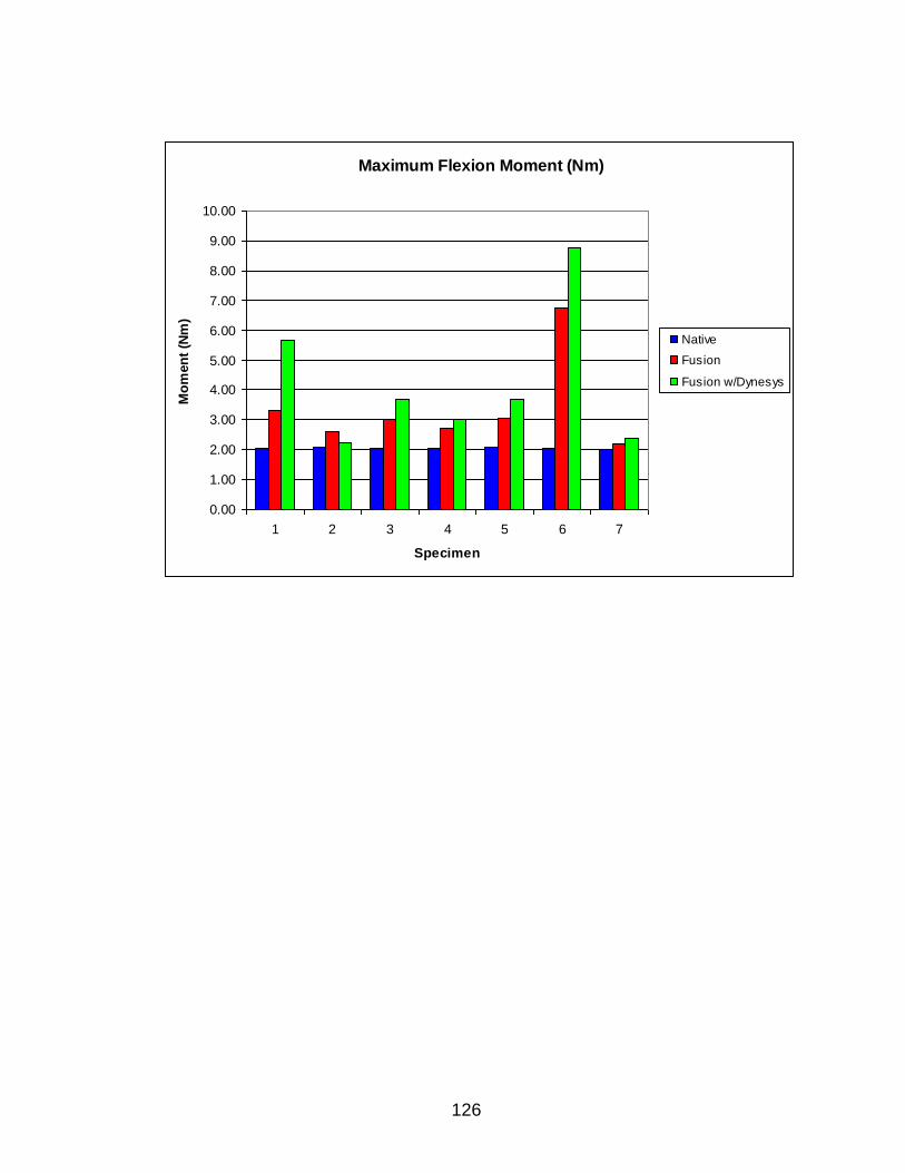
126

Maximum Flexion Moment (Nm)

0.00

1.00

2.00

3.00

4.00

5.00

6.00

7.00

8.00

9.00

10.00

1 2 3 4 5 6 7

Specimen

Mo

men

t (N

m)

Native

Fusion

Fusion w/Dynesys

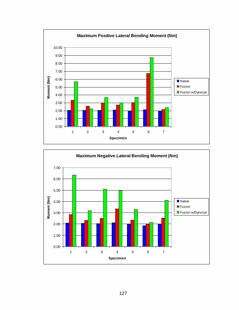
127

Maximum Positive Lateral Bending Moment (Nm)

0.00

1.00

2.00

3.00

4.00

5.00

6.00

7.00

8.00

9.00

10.00

1 2 3 4 5 6 7

Specimen

Mo

men

t (N

m)

Native

Fusion

Fusion w/Dynesys

Maximum Negative Lateral Bending Moment (Nm)

0.00

1.00

2.00

3.00

4.00

5.00

6.00

7.00

1 2 3 4 5 6 7

Specimen

Mo

men

t (N

m)

Native

Fusion

Fusion w/Dynesys