In the last session we introduced the firm behaviour and the concept of profit

maximisation. In this session we will build on the concepts discussed

previously by examining cost structure, which is a key component of profit

maximisation. Irrespective of the size of the business, all firms, whether it is

Mercedes Benz, Nestlé or the corner store in our suburb, face a common

concern of costs. Focussing on costs will also provide a deeper understanding

of the firm’s supply function.

1

As discussed earlier Profit=Total Revenue – Total Cost; where total revenue is

simply price times quantity or the amount a firm receives for the sale of its

output. For the moment we will focus on the perfect competition. Let’s say that

a Primo pizza factory in Italy sells 500000 pizza and average price of each

pizza is €5, the total revenue will be 5 × 500 000 = €2.5 million.

To find profit we also need to consider the costs side of the equation. To

produce pizza, Primo will have to incur a range of costs such as employing

labour, buying machinery, paying rent, servicing equipment, buying ingredients

etc. These represent the total costs of Primo factory.

Profit is a firm's total revenue minus its total cost. That is:

Total revenue is often expressed as TR and Total cost as TC. The greek letter

pi (π) represents profit.

π = TR – TC

2

As expressed earlier, costs in economics represent opportunity costs.

Opportunity cost of something is what you give up to get it or the value of the

next best alternative forgone.

Sometimes opportunity costs are clear but sometimes they can be tricky to

spot. For example, if Primo factory obtains flour of €1000 then this amount

cannot be used for anything else or €1000 has to be sacrificed to obtain the

flour. Thus, €1000 is an opportunity cost. Because this cost requires firm to

pay out money, it is an example of explicit costs. Opportunity costs sometimes

do not require a cash outlay. For example, if Primo is a skilled computer

programmer and could earn €100 per hour working as a programmer but

chooses not to do so and instead uses the time to manage the pizza factory.

The €100 forgone is also an opportunity cost and is classified as implicit costs

as it does not require any financial outlay.

3

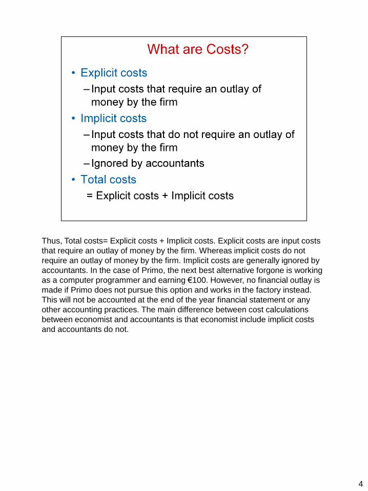
Thus, Total costs= Explicit costs + Implicit costs. Explicit costs are input costs

that require an outlay of money by the firm. Whereas implicit costs do not

require an outlay of money by the firm. Implicit costs are generally ignored by

accountants. In the case of Primo, the next best alternative forgone is working

as a computer programmer and earning €100. However, no financial outlay is

made if Primo does not pursue this option and works in the factory instead.

This will not be accounted at the end of the year financial statement or any

other accounting practices. The main difference between cost calculations

between economist and accountants is that economist include implicit costs

and accountants do not.

4

One of the most important implicit costs that most firms face is the opportunity

cost of capital that has been invested in the business. For example if Primo

used €300 000 of his own money to start up the company, then the interest

forgone on this money is part of implicit costs. The reason is that Primo could

have used this money to earn interest in the bank. So the forgone interest is

an implicit opportunity cost. This implicit costs are included by economists but

not shown as costs in standard accounting practices.

5

Because economic costs are different from accounting costs, there is a

difference in calculating profit.

Economic profit is total revenue minus total cost; where total costs includes

both explicit and implicit costs.

Accounting profit is total revenue minus total explicit cost.

6

Because accounting profit does not account for implicit costs, it is larger than

economic profit as shown in the slide above. As shown in the graph above the

total costs are much greater in the economists view of the world rather than an

accountants.

7

We are now moving on to the production side of firms operation.

Production function captures the relationship between the amount of output

that can be produced given the factor inputs. Factor inputs include land and

labour, capital. We will mainly focus on two factor inputs, capital and labour.

Some firms like car manufacturing require very large amounts of capital

whereas the others such as teaching tend to be more labour intensive.

The production function is an engineering relation that defines the maximum

amount of output that can be produced with a given set of inputs. The

production function is represented as Q=F(K,L). How land and labour can be

combined to produce any good depends on the technology available for

production. Technology summarises the know-how available at a given time to

convert raw materials into output. Lets say that the two basic factors of

production are capital (for e.g. machines) represented as K and labour

represented as L. The combination of these inputs are used to produce a

certain amount of output. Amongst other things, technology is a key factor in

how labour and capital are converted into output. For example, technology

summarizes the feasible means of converting raw inputs, such as steel, labour,

and machinery, into an output such as an automobile. An alternative way of

8

thinking about technology is “engineering know-how”.

While deciding the optimal amounts of labour and capital to use, managers are

constrained by time frame. In the short run some factors of production are

fixed. For example, the size of the car plant is fixed in the short run. However,

labour can be more easily altered. In the long-run, both capital and labour are

variable factors.

Short-run

Period of time where some factors of production (inputs) are fixed, and

constrain a manager’s decisions. For example, building a car assembly

line takes several years.

Long-run

Period of time over which all factors of production (inputs) are variable,

and can be adjusted by a manager

There is no fixed time period known as the long run and will vary from

business to business. For example, for a restaurant owner the long run may be

a few months but for a steel factory the long run may be several years.

Typically labor is a variable factor and capital is fixed in the short run .

8

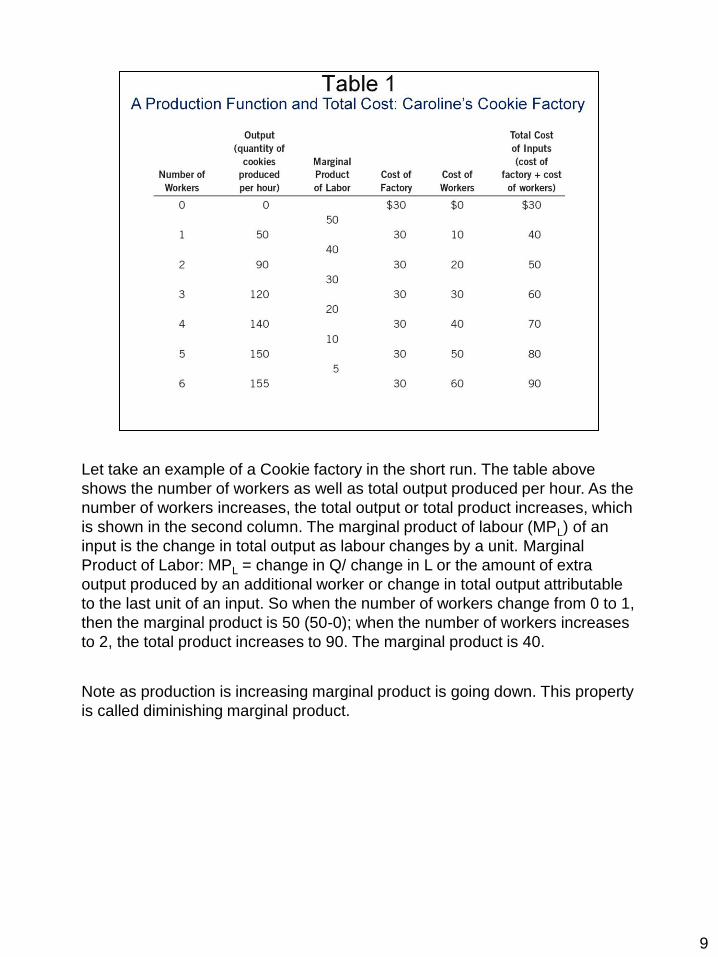
Let take an example of a Cookie factory in the short run. The table above

shows the number of workers as well as total output produced per hour. As the

number of workers increases, the total output or total product increases, which

is shown in the second column. The marginal product of labour (MPL) of an

input is the change in total output as labour changes by a unit. Marginal

Product of Labor: MPL = change in Q/ change in L or the amount of extra

output produced by an additional worker or change in total output attributable

to the last unit of an input. So when the number of workers change from 0 to 1,

then the marginal product is 50 (50-0); when the number of workers increases

to 2, the total product increases to 90. The marginal product is 40.

Note as production is increasing marginal product is going down. This property

is called diminishing marginal product.

9

Diminishing marginal product emphasizes that the marginal product of an input

declines as the quantity of the input increases. If you take labor as the main

input in production, then the property of diminishing marginal product implies

that as we hire more labor units, the extra output or marginal product received

by employing each extra labor unit decreases. Again be very careful as we are

talking about marginal product, not total product. To simplify things lets take an

example. Lets say that a coffee shop opens on campus. The coffee shop

provides coffee+cake+sandwiches. At first there are only two people working in

the coffee shop who run around and do everything. However, they struggle

during peak lunch hour. So they employ another person. The extra output we

get from the third increases but does not jump as dramatically as when we

increased employment from one to two people. Thus marginal product

decreases. Now we continue hiring more people. As more people come into

the coffee shop there is less room for people to specialize. The total output

increases but not as much. Thus, marginal product is going down. The same

applies to Caroline’s cookie factory or any other business. As we keep

increasing our inputs, there comes a point when the extra output contributed

by each worker starts to decline. This is also reflected in the slope of the

production function. As we employ more inputs, the total product increases

sharply but then the increase slows down as diminishing returns set in. The

point at which diminishing returns set in will vary for different businesses.

10

The total cost curve and production function are opposite sides of the same

coin. The total cost curves get steeper as the amount produced rises. Why?

Essentially because of diminishing marginal product. As we hire more workers,

the kitchen used for production of cookies gets more and more crowded. The

workers are getting less productive as we produce more. Thus, producing one

additional unit of output requires a lot of additional units of inputs and hence

there is a steep rise in costs.

11

The production function in panel (a) shows the relationship between the

number of workers hired and the quantity of output produced. Here the number

of workers hired (on the horizontal axis), and the quantity of output produced

(on the vertical axis). The production function gets flatter as the number of

workers increases, reflecting diminishing marginal product. As we employ

more inputs, the total product increases sharply but then the increase slows

down as diminishing returns set in.

The total-cost curve in panel (b) shows the relationship between the quantity of

output produced and total cost of production. The total-cost curve gets steeper

as the quantity of output increases because of diminishing marginal product.

The workers are getting less productive as we produce more. Thus producing

one additional unit of output requires a lot of additional units of inputs and

hence there is a steep rise in costs.

12

We continue our examination of costs but initially from the short-run

perspective. We have two types of costs- short-run and the long-run costs.

Short run is the period when only some inputs are variable and we are stuck

with existing levels of fixed inputs. In the long run all inputs can be varied. So

lets begin by various types of costs in the short run. The costs that vary with

output are variable costs or VC(Q). Variable costs increase as output

increases. The costs that do not vary with output are fixed cost or FC. And the

sum of variable and fixed cost is total cost. Fixed costs do not change as

output changes. Example includes the leasing costs of land, machinery or a

factory.

13

Now we have some more definitions. Average fixed cost (AFC) is defined as

fixed cost divided by the number of units of output. Fixed cost do not vary with

output but AFC declines as more and more output is produced.

Average variable cost is variable cost divided by the number of units of output.

14

Average total cost, ATC:

Total cost divided by the quantity of output

Average total cost = Total cost / Quantity

ATC = TC / Q

Average total cost is the cost of the typical unit if the total cost is divided

evenly over all the units produced.

15

Marginal cost is the cost of producing an additional unit of output. Typically

marginal cost increase as production increases. Why? The answer is

embedded in the concept of diminishing marginal product which emphasizes

that the marginal product of an input declines as the quantity of the input

increases. If you take labor as the main input in production, then the property

of diminishing marginal product implies that as we hire more labor units, the

extra output or marginal product received from each labor unit decreases.

Again be very careful as we are talking about marginal product, not total

product. To simplify things lets take an example. Lets take the example of

coffee shop again.

The coffee shop provides coffee+cake+sandwiches. At first there are only two

people working in the coffee shop who run around and do everything. Lets say

they struggle during peak lunch hour. So they employ another person. The

extra output we get from the third increases but does not jump as dramatically

as when we increased employment from one to two people. Thus marginal

product decreases. Now we continue hiring more people. As more people

come into the coffee shop there is less room for people to specialize. The total

output increases but not as much. Thus, marginal product is going down. So

what we have here is that marginal product is going down, which essentially

implies that marginal cost is going up. Why are the two related? Because each

16

additional worker is able to contribute less to the total cups of coffee in this

instance, but takes essentially takes the same wage. What this means is that

value of the product contributed by each additional worker is reducing but the

wage is not. Therefore marginal costs are increasing. Don’t confuse marginal

costs with average costs here!

16

Lets take an example of Conrad’s coffee shop to understand the cost

structures better. The fixed cost in this case is the rent on the rent of the coffee

shop, which is $3.00. As discussed previously, variable costs change as output

changes. In the above case the variable costs include milk, sugar, beans,

workers salaries etc. As the number of coffee produced increases, the variable

costs go up. Total cost is the sum of the fixed cost and variable costs. Marginal

cost is the change in total cost/change in quantity. So lets say we move from 0

to 1 cups of coffee. The marginal cost is $0.30 ($3.30-$3.00). Now if output

increase from 1 to 2 cups of coffee; the marginal cost is $0.50 ($3.80-$3.30).

Thus, MC increases as we increase production. Also note MC is not the same

as ATC.

17

Here the quantity of output produced (on the horizontal axis) is from the first

column in Table 2, and the total cost (on the vertical axis) is from the second

column. As illustrated, the total-cost curve gets steeper as the quantity of

output increases because of diminishing marginal product.

18

This figure shows the average total cost (ATC), average fixed cost (AFC),

average variable cost (AVC), and marginal cost (MC) for Conrad’s Coffee

Shop. All of these curves are obtained by graphing the data in Table 2. These

cost curves show three features that are typical of many firms: (1) Marginal

cost rises with the quantity of output. (2) The average-total-cost curve is U-

shaped. (3) The marginal-cost curve crosses the average-total-cost curve at

the minimum of average total cost.

As discussed earlier marginal cost rises output goes up due to diminishing

marginal product. Average variable costs also rises because of diminishing

marginal product. The shape of average fixed cost is straightforward as well.

Average fixed cost (AFC) is defined as fixed cost divided by the number of

units of output. Fixed cost do not vary with output but AFC declines as more

and more output is produced.

The U-shaped ATC requires some explanation. The ATC curve is essentially

linked to MC curve.

When MC < ATC: average total cost is falling

When MC > ATC: average total cost is rising

19

The marginal-cost curve crosses the average-total-cost curve at its

minimum

This mathematical relationship applies in all scenarios. Lets take an example.

Say you have a distinction average and get a pass in this course. The

marginal mark is now pass. What will this do to your average- pull it down.

Similarly when marginal cost is below average total cost, ATC goes down.

Now take the scenario when you have a overall average of pass and you get a

high distinction in this course. What will this do to your overall average?

Possibly pull it up towards a credit. Similarly the average cost increases when

marginal cost is above the ATC curve.

The marginal-cost curve crosses the average-total-cost curve at its minimum.

19

Many firms experience increasing marginal product before diminishing

marginal product. As a result, they have cost curves shaped like those in this

figure. Notice that marginal cost and average variable cost fall for a while

before starting to rise. This occurs because initially when we hire more people,

there is room for specialization. As people specialize in different activities,

marginal product increases. The gains to this eventually fade away leading to

increasing marginal costs. Again think of the coffee shop example. If there is

only one person in the coffee shop who does everything, he/she is unlikely to

be very productive. However, hiring one more person allows the two workers

to focus on separate activities, improving the output/customer service etc.

dramatically. Hiring a third worker may not have the same sort of dramatic

effect though.

20

So far we have looked at the firms short run cost curves. The firms in the short

run have fixed costs but in the long run all costs are variable. The firms have

greater flexibility in the long run and can change all inputs of production.

21

In the long run the manager can change the plant size, labor, get new

machines etc. So in terms of costs, the manager is faced with Long-run

Average Cost (LRAC) curve which is a envelope of all the short-run average

cost curves. The bold red line on the diagram is the long-run average cost

curve facing firms in the long-run. So basically what we have here is that the in

the long run firms can alter all the inputs of production and is not restricted to

just labour. LRAC is composed of SRAC curves corresponding to different

plant sizes. In the long run firms pick the best short run curve corresponding to

a particular level of output. The U-shape of the LRAC curve reflects the

principle of Economies of Scale and Diseconomies of Scale. Economies of

scale occurs when LRAC declines as output increases or average costs

decreases as output increases. Diseconomies of scale occurs when LRAC

goes up as output increases

Economies of scale

Long-run average total cost falls as the quantity of output increases.

This is the most common type of phenomenon. As plant size increase,

average costs fall due increasing specializations.

Constant returns to scale

Long-run average total cost stays the same as the quantity of output

22

changes

Diseconomies of scale

Long-run average total cost rises as the quantity of output increases.

This occurs if the firm gets so big that it increasingly runs into

coordination problems. This is not commonly noted in the real world as

recent times have shown that firms are adept at coordinating large

scale operations across national borders.

22

We end this session with a summary of the definitions of cost curves to refresh

your memory about what we learnt in this session.

23