TitleIn Situ Determination of Variation of Poisson's Ratio in GraniteAccompanied by Weathering Effect and its Significance inEngineering Projects

Author(s) KITSUNEZAKI, Choro

Citation Bulletin of the Disaster Prevention Research Institute (1965),15(2): 19-41

Issue Date 1965-11-30

URL http://hdl.handle.net/2433/124701

Right

Type Departmental Bulletin Paper

Textversion publisher

Kyoto University

Bulletin of the Disaster Prevention Research Institute Vol. 15, Part 2, No. 92, Nov., 1965

In Situ Determination of Variation of Poisson's Ratio in

Granite Accompanied by Weathering Effect and its

Significance in Engineering Projects

By ChOrO KITSUNEZAKI

(Manuscript received September 30, 1965)

Abstract

At first, the practical method for the generation of S wave was examined in the adit. A small explosion in a drill hole was mainly used as its wave source. The small explosion can be approximately considered as the single force referring to the effect on the generation of S wave.

Secondly, real measurements were carried out in order to determine the ratio (a) of P wave velocity (V „) to S wave velocity (Vs) in granite. It was approximately expressed by the following formula.

a= — 0.49T71,+ 4.34

where V„ Ckm/secD is the value which varies by the weathering effect. It is suggested by this result that the well-known discrepancy between dynamic Young's modulus and static Young's modulus, in situ, can be explained by neglecting Poisson's ratio variation in the estimation of dynamic Young's modulus, and partly by insufficient evaluation of the velocity lowering in the adit wall.

§ Introduction

Determination of elastic constants of rocks is ofen required for designs in civil engineering. Seismic prospecting is applied to measure elastic constants of rocks in situ. The most important advantage of this method is that physi-cal properties of rocks in a wide and deep range can be measured in its natural conditions. However, it is generally recognized that Young's modulus determined by this method is different from one determined by the direct mechanical method, the jack method."--3) For convenience we shall call the former the dynamic method and the latter the static method. The values found by the dynamic method are larger than those by the static method. According to several reports1"), the ratios of these were about four to five. Many ideas were proposed to explain this problem. However, little attension has been paid to the physical basis for the determination of Young's modulus, that is, the assumption on Poisson's ratio.

Properties of isotropic and elastic materials can be represented only by two constants. Two elastic constants can not be determined by one value. So, an assumptive value has been used as Poisson's ratio for the estimation of Young's modulus, because the kind of the seismic waves whose velocity can

20 C. KITSUNEZAKI

be practically measured has been considered as only P wave. Here is one

problem in the validity of the assumption for Poisson's ratio. Between P wave velocity Tip, S wave velocity Vs, Poisson's ratio a, density p, and Young's modulus E, is the following relation,"

pi7,2f(a) (1)

where

(1+ a) (1 —2a) Au) =(2) (1—a)

a2-2 a =(3) 2 (a2 — 1)

If we take V„/Vs in place of a,

E=pV,2F(a)x1011)clyne/cm2 (4)

=1 .02p Vp2F(a) X 104kg/cm2 (engineering unit)

where

a=17„/Vs, Vp—Ckm/sec) p—Cg/cm3) (5)

3a2-4 F( a)== a2(a2 _1)=f (Q) (6)

The relations between a, a and F(a) are shown in Fig. 1. Existence range is 0 to 0.5

for a, 1.414 to co for V,.

Fia) • 0.4In general cases,"-4)Pois- son's ratio a is assumed 0.3 as 0.25 (V„=1.73), dis-

Q5

regarding diverse states az

Raiof rock. This figure is 0.1 valid for the materials in

the interior of the earth, 00

and the laboratory ex-

1

a, ^/,_ periments" for rock speci- vs mens revealed an appro-Fig. 1 Relation between Poisson's ratio a, F(a) and a. ximate validity of this

figure. Usually, however, the laboratory experiments are carried out not for weathered rock specimens with cracks, but for sound rock specimens. Can the application of this figure be extended to the rocks in natural condition, based only on such laboratory experiments ? If this assumption is not valid, considerable changes are possible for the estimated Young's modulus (Fig. 1). For this reason, the author intends to measure Poisson's ratio in situ. As known from Eq. (3), Poisson's ratio can be determined by the measurements of P wave velocity and S wave velocity.

§ Experimental field

Experimental data in this paper, unless otherwise specified, were obtained in the field experiment at the geological survey area for the construction of

Determination of Poisson's Ratio 21

a power plant in the Tsuruga Peninsula, Fukui

Prefecture, Japan. The place is situated in a

granitic zone. Geological survey classifies the rock of the experimental field to granite, T

granite-pophyry and aplite. But the detail of zoning may not be necessary at the present

k.

stage of discussion. In this paper they are.0

simply looked as granite. The position of the u cv ,g i field is marked on the map in Fig. 2, as well as a few other experimental fields cited in this paper. The rock is characterized by development of a regular joint system, dominantly striking N65°E and dipping 74°SE. Fig. 2. The places of experimental Shear zones also tend to dominate along thisfield.

plane. The experimental works were carried T : Tsuruga (main field). out in the exploration adit, about 20m below I : Ikoma LT : Ushimado. the mean sea level and about 25m-70m below

the ground surface. The

IL G map of the adit is shown

.1,,.,i.in Fig. 3. The classifica- ;,„,:,,,,,..071G-••-tionof the feature of rock i.•=specified in the map is

Jo,,.!•

..,:i. cited from H. Tanaka's

A , GO , `.., . I

4 4

Do

'I

4/01°)1(030m.

1

['-i C. Fa CL I ShowzonegEggDsurvey (see, Appendix). Seismic velocites were measured in the rocks of I CH variable state—sound to weathered.

-,3 0.2 — q4—mm. c Fig. 3. Geological condition of the experimental field (adit).-40.,4111160„em.°

G: granite. Gp: granite-porphyry.> wirmimeal .ut-2

_

.mriaraz•zwri A; aplite.---boundary of rocks. '1%//.iii.

W

§ Experimental apparatusAIIMIIII•Mi iro1E111 A conventional recording system consisting of 0.0

ial 100I300 geophones, an amplifier and an electro-magnetic —> f (cps) oscillograph was used in this experiment. How- ever, each unit was selected considering theFig. 4. Frequency characteris- tics of the geophone. speciality of the work. The geophones, NEC VP-225, have natural frequency of 25cps and can be used for the detection of horizontal vibration as well as vertical vibration. The amplifier, ST-2600A, is a transistorized one (12 elements) manufactured by TOkyei-Shibaura Electric Company at the special order of our laboratory. Its important characteristics are as follows. .Amplifing range covers relatively high frequency one, 30-3000 cps, and multiple filter units of high and low cut are set. Consideration is

paid to the accurate measurement of wave form and amplitude.

22 C. KITSUNEZAKI

`Ne.43.4^410'N.' -•

)111i oAffS#Ii ot

to to. to.

----)•Frequency(CPs)

Fig. 5. Frequency characteristics of the amplifier.

Frequency characteristics of the geophone are shown in Fig. 4, that of the amplifier in Fig. 5.

The electromagnetic oscillograph 17 (102A, Sanei Company) was driven

M : at the maximum paper speed ,

a 1m/sec. Accurate 1000 cps signal controlled by piezo-mechanical

-11]1)b fork was used for precise meas-

.

urement of time. In many cases, galvanometers of 500cps in

10 100 1000 the natural frequency were used, f(CPS) except for a few cases in which

Fig. 6. Resultant frequency characteristics of 2000cps galvanometers were tried. the recording system. Generally in this experiment the

M: relative magnification (amplitude/velo— rock condition was so bad that city). resonance-like oscillation of cracked

(a) no filter, (b) high cut : 2. rocks on the adit wall obstructed

normal detection of high frequency seismic waves. For this reason high fre-

quency waves above 200cps could not help being cut in order to detect S wave. Accordingly, high frequency galvanometers were not necessary. Resultant characteristics of the apparatus, from a geophone to a galvanometer, are demonstrated in Fig. 6. The records used for the following discussion on wave form characteristics of S wave were obtained in the condition of curve (b) in Fig. 6.

§ Generation of S wave

In previous works78), the author revealed S wave can be generated by a small explosion. The condition of seismic works in a adit protects the recognition of S wave from the obstacle of surface wave. For one record, a single drill hole, 0.7-1m in length, 3.6cm in diameter, was used as the shot hole. The shot holes were drilled horizontally and perpendicular to the adit wall. They are illustrated in Fig. 7. Geophones were installed on the pick-up bases cemented in short drill holes on the adit wall. Three elements ob-servation of the oscillation could be made by setting three geophones on the

Determination of Poisson's Ratio 23

R

\2, I \I c wc

''.,,,I te 5A .M4Ylok,,)*.)*;w.„,. 4.4, iiMINNEMMIIIRts„.,.,,1 ‘3'MAMICSIDIMill .et------e4,77z•-,.. ,ice` 4,./ 70^400-- "9 7.-C-6-L T

(cm) ,----- 40 , o 10 cn Fig. 7. Sketch of the shot:hole. Fig. 8. Sketch of the geophone setting.

C : charge. C: cement. R : rock. V, L and T : W : water pouch. vertical, longitudinal and transverse

component.

T L

Hi , . ,i„I, IA i1, No 50 t1\fkri,v4....y.4, / f •P i , , ' ,.,

2 ., , I •^ V

3 . o • / -5 •

5 . ,,, \r"1./k/ \IO.esr."1 4 -4. ' i ,, f,, ,

5 ,,/"\I=,, 5,,k:^n_ 16ft‘' —G...ti-t\i^

,{ v% ury, \ /Vv. 7 4' '' \ I \ I. k' 14*-1"'MA\ /1'' "4"' V, ,i ft" ,04#411 .4.,...1-414 v" \ ,.,",,,,S,

,

aL Jo 10011 ifte ,0 .., , T 1 r , ,' ,

I All ' * i jvV\r"*"4' 12 12 'p Ir".' ' " i ivrii\CY

Fig. 9. Examples of the records. (explosion)

I I I I I

P S S/ V *.16W g, T &

,) 20 ------------, P — " T 2.4 •.-io--+L

V,tor)

L

\„

L r

r. o. T + / T

_t ta S/

V

is v 19r----:::--„, - , 1, L . p,

>t,

1 1 1 1 1 . '1--'

P

10. ILI / T

Fig. 10. Examples of the motional orbits. (explosion) - - - - P wave , S wave.

24 C. KITSUNEZAKI

pick-up base. Details of geophone setting are demonstrated on Fig. 8. Fig. 9 is an example of records obtained in the usual seismic line, in which

case the geophones and shot point are located on the same straight adit. The motional orbits obtained from direct plotting of the records of the same

kind are demonstrated in Fig. 10.

4it I A,*

a p

6- t ^ JP

N 6

/ ;I\oki P:\vj

20m /2 # 12

Fig. 11. Spread of geophones and a Fig. 12. The records obtained in the shot point for the experiment of condition of Fig. 11. (explosion)

S wave.

Although ideal orbits of wave phases can not be obtained, owing to the

surface effects of adit wall, it is recognized that the principal direction of "P

phase" oscillation is longitudinal and in many observational points the princi-pal direction of "S phase" oscillation is nearly perpendicular to the former. Another evidence shows "S phase" is S wave. Fig. 11 illustrates the experi-

mental procedure. Fig. 12 is the record obtained in this condition. "S phase" is clearly body wave because the propagation of this phase is not limited only in the near-surface of the adit.

Directional characteristics of emission

of S wave are an interesting problem in

order to analize the mechanism of genera- \ tion of this wave . The complete radiation \

_ _ _ _ — — — pattern could not be obtained, because

the field conditions were not adequate for this experiment. However, it is apparent

that this wave has the polarization char-

acteristics shown in Fig. 13, by synthesiz-Fig. 13. Radiation pattern of S wave ing the separate experiments whose

generated by the single force to which examples are shown in Fig. 14. Initial the effect of the small explosion iglus- motions of S wave demonstrated in Fig . 14

trated in Fig. 7 is looked as identical, mean only qualitative tendency of these

regarding the generation of S wave. directions, because T and L records were

separately obtained.

Determination of Poisson's Ratio 25

,..,,

>,.., sti

161,,16 8

T T,' J ,1\..------

- 1 -2--!-----\, a_„,.. ,'AR" .. io'1'4,10"--- .,,,,

,

20

ti----,\,(v\,-4/-•,

1 IrtVI:.....u.....4.........N,:il,,,,....._ f-ev\2012,A ;, II (\e....../. p s p% \• ' '',

. -

16 . 4 IS 1_1,004 a A b

y N I , A, , L i .,,::,. ,vii i .,t,.,.

,

s,...„....„

.

.., s;:, ., P s : 20 ,..,..t,„+,,,v11 * fir: ft 1 ' S \._ -4".4, ' t ti` ark, p w .,

II

H 1 12] 1, 41. I L__ _J I J 1 - '

,. 16 16,

—11C‘ 1.tom.''-17.,!T 41if \

-T(-.'‘TFt'

Iti 0tiO_7\*.G1 —1 I 0 20 • ^—..s.—s

Fig. 14. Examples of records showing initial motions of S wave radiated from the small explosion.

Characteristics : G: - L ; (a) of Fig. 6, others ; (b). --. - - initial motion of S wave .

This means the origin can be

regarded as the single force"<-), as .,iii—DI— -—4-07+ I . far as it concerns the generation

of S wave. This circumstance is I 'V , illustrated in Fig. 15. Namely, thes1.p..-1 I

--I weak explosion (dynamite, 5-30g,

I'k 1 F, in this experiment) in a hole canS

be approximately treated as com- Fig. 15. Illustration of the mechanism of wave bination of an equi-expansive source generation by a small explosion. A small ex-and a single force. By the latter plosion in a hole can be approximately treated S wave can be generated. In thisas combination of an equi-expansive source case, the effect of the explosionand a single force. will be equivalent to the effect of a hammer blow on a rock wall. Experi-ments showed that the records obtained by the hammer blow are nearly the same as those by the explosion. Examples of the records demonstrated in Fig. 16 show that the reverse of polarization occurs by reversing the direction of the hammer blow.

In the present experiment, S wave could be easily generated by the explo-sion in sound rocks. In cracked and weathered rocks, S wave was not domina-

26 C. KITSUNEZAKI

2 No.22 SM 194S.

3 2Tr

•

io4 " 5"T 2420 20 19 111'

6

19, T (\..7\/

19 20T

111 8 1T 14

.9 T . P II O_ A_ _g2, ,0fOT

T

P S P S /2 A (No 90) B (No.01) p S

Fig. 16. Records obtained by the hammer blow. Fig. 17. An example of the records obtained Phase of S wave is reversed by reverse of in the weathered rock. (spread : C2 - El

the blow direction. line)

ted by this method. This is due to the fact that the propagation of the waves was effected by the inhomogeneous states of the media. In this condition, even P wave was strongly disturbed as to its travel time and wave form. Noise-like oscillations, which appeared to be generated by the propagation along ir-regular wave paths and conversion of waves in inhomogeneous media, obstruct-ed the clear recognition of S wave. Those examples are shown in Fig. 17.

If the wave source purely originates only S wave, the circumstance will be much

improved. For this purpose another me- thod was tried. Fig. 18 illustrates this.

A wooden plate is pressed with two jacks

P on a concrete base which is made in order to level a rock surface. This is struck

with a hammer in the direction parallel 71 NT,pkC % to the plate surface. Even by this method,

Fig. 18. Illustration of one of the me- generation of P wave can not be avoided, thods tested for the generation of S but its proportion is much decreased ,

wave. in comparison with that by the explosion P : wooden plate, 5 X 36 x 200cm. method . In sound rocks, the wave trains I

: jack. of the transverse component obtai ned by C : concrete floor (10cm thick). thi

s method practically begin with S wave. Such circumstances as this are demonstrated in Fig. 19.

In cracked and weathered rocks, the records are improved by this method only somewhat (Fig. 20).

Velocity of S wave was measured principally by the explosion method and

partly by the plate-blow method. In many cases, velocity of P wave is also easily determined from the same records as ones for S wave. The measure-ments were carried out on the rock of every condition in the exploration

adit.

Determination of Poisson's Ratio 27

1 t 1o.61 ,'A' ;' P

412, ,_•AILi L4`.,.,), 43 P .,P---N .2..i- t ,- 4' v`,`

1,I i A 3-••^•• .44. a . n <1..4 . 3 i. ,r ,,, 4h e j , R: rz't ' ' _.4L 4., ,., ,,,, .

c, 1 5 , stAk ../"`, , 6T 3, n , 1\,..."------ „ Ct.. 4. ._,,,,,,,../rs...........„,_,—\ 4-16v

4;7IT4' j L ot, A .''',.\ .."..--.---...---- 8. %s, 4

4.9 , IOT T '-------." \ I (+S.'-''....."-...'.- '..-..

.

, ..,., _22,4,1 ,./,. , \ .,.........„....... 44I. II T 1.SO:,,,,,

EE 12 12 Tet, (s\rs„....„....., 16 r.r.

_

I I t.,..4.. /.......---,,..-

P'S \ 1

Fig. 19. Examples of the records obtained in sound rock by the method illustrated on Fig. 18. (source ; Pi , geophone spread , HI- J1 line)

§ Determination of wave velocitiesN_at t ,I e' P g,„s ,..Ak_...„" 4 ̂c-^-

Method of analysis 7 -...__ T ../,..

3-.... --,__--- (1) A troublesome problem in the de- termination of wave velocities is on the 5L.t....+4______,„,....____ effect of the surface layer surrounding :: 6L,1,_..,h______,:__________

!,L„........4.,______,___._._ the adit. The layer of this kind is made`,.\ TILI__,,,,,_......_.,..........„.____ 41 secondarily by the effect of the adit ex- ''',BT cavatio n. This layer is cracked and in , sa 8L._t...........t..--..„----

some cases weathered. So its wave velo- Fig . 20. An example of the record ob-cities are lower than those of undisturbed tained in weathered rock by the me-rock surrounding it. For the determina- thod illustrated on Fig. 18. tion of the velocities in undisturbed rock, (source , P2, geophone spread ; El - F1 the refraction method is useful. If the line)

.

---. Vi V2 ..7, t

2 s'--. -----.. .- t ' t4.,.../ X t

y„ C.T---/xx --.oix--------....-- x. x.x--.),-,„ ,-V1

-----,"-,,, t .xs,I2.. \V / JV •t , .1.; ''),,,,,./•

v2x ,x . . _

r . ±......„-----''M F A P Bh

x Y ) Vi

Ali VI ho •:

VI '-------- — ,______,_____..,-------=' —__^ T V2hV2

Fig. 21. Illustration of the "Hagiwara's Fig. 22. False application of the "Hagi- method"wara's method". F

: false, Vi<V21<V2. T : true, zit= (4+ ty— tz)/2, h =I)1dt/cos° .V 2 ; based on Vil", V2- and VI.

28 C. KITSUNEZAKI

effects of the surface disturbed layer are not completely eliminated from the observed travel times, errors are more or less conducted into the analized velocities. The "Hagiwara's method"" is very useful for this analysis. This is the well-known method to eliminate the effect of the surface low velocity layer and to determine its thickness and the velocity of the under-lying high velocity layer. The outline of this method is illustrated in Fig. 21. For the application of this method, the seismic line should be long enough that refraction ranges of the waves originated by the two end shots widely overlap. In the short seismic line, identification on the direct and the refraction

wave ranges is often so difficult that the results of analysis tend to contain error, owing to the incomplete separation of the ranges. This circumstance is illustrated in Fig. 22. On the determination of the velocities, the author was careful about this fact. When the "Hagiwara's method" cannot be applied, the ordinary analysis in case of two layer based on the assumption of monocline dip is adopted.

The analysis was done by the two method mentioned above. It was the author's principle to adopt the same method in the analysis for both P and S waves on the same seismic line. This is based on the assumption that there are not considerable differences between the structures for both P and S waves. In this paper, the most important quanta which can be experimentally obtained are the ratios of P and S wave velocities. Even if the adopted analitical method had not been adequate and therefore the absolute velocities determined by it had been somewhat erroneous, it should have been avoided that the determined a contained considerable errors based on different ten-dencies of analitical results. In this experiment, the travel time curve was often so complex owing to inhomogeneous properties of rocks, that this was necessary for useful analysis.

(2) In a curved adit, geophones and shot points can not be located on a straight line, that is, the seismic line is curved. For the analysis in this case, the "Hagiwara's method" was modified as follows. In Fig. 23, the curve APB is a seismic line. A and B are shot points. P is one of geo-

.

hp

i max,

A

14—(x-y+z) 2(y-x+z)—>i"71115 . 77/0IP 1

7////////// V2

x

4.

A

Fig. 23. Analysis on curved seismic line.

Determination of Poisson's Ratio 29

phones. We shall assume o 2 I ^ i

that projection of an in- '•.Ig dividual wave path to the

plane containing the seis-_ti mic line (usually, horizon-Ix kJ tal plane) is practically a .4 1 ' = rvi 7,

straight line. It meansa.(Y, _ ---(0 -o

that the direction of layer- (•-.e•J - .; 2

_ ing effective to travel time2 bq ..- ..../

cR Lc;"0

of the waves is normal toMsr0 1- 0

the plane containing the 1‘ 2aii „,

seismic line (horizontal11I .,--t-',I,N\ 0.. 1 / plane) as in the case of , 1.i 0 1-•:,- the ordinary seismic pro-,1A.-,II

\, .Ln specting on the groundk ..10• •:r

\l',,/0 surface. The second mean-\/,..•• 02 Io,,

ing of this assumption is 1- °' Q•

that the boundaries of1 ic,‘ -0oe different media are nearly \1.110rxl

normal to wave path and' I 2 \ ‘-, •

. :

therefore the variation oftet • z & )

-

/Ktto ,(., the rock velocities can not\ ,.\ ._+ 4iP•, be exactly evaluated in \• ^ /\ 4.: !,

the region near a con- \/ , ..._. siderably curved seismic4:i

i .\1 line. If the thickness of \. • r--.4-33 „,0

''•',,-`

,z,F)

the surface layer is as,I;•i,A ; / -0••I

u

\li sumed to vary gently, aso in case of the ordinal i0. \A/I.Q-' /

\I‘5 I "Hagiwara's method", /.,

-

.- 0 4 -̀'I 0 ; . zit= tx+ty — tz ir v, 2/

\(z-•-," 1 h„ cos 0j \,,I

0

— ,-4i Vii I \1

x+y—z ,I'\1 ,c,— tI L. +(7)://\ o 2 V2; /\trl U . \ =1

E -IF 914\1^ x 2V2= — zlt= x— y+ zdI S2 i1 7") ' ,T5

I hA cos 0l' .\.cz 1....-- + (8) 11 V

I !9,.0 '„:.' 1 •9 1

s where tx, ty and t2 are the\o- '„, A7.(

,,,.; travel time of refraction dg?el`,.P. wave in x, y and z, re- / / / b \ . c,1• 1,2.0 spectively. hp and hA are4.". the thicknesses of the sur-face layer of positions P 4 ' b' ' A L - - '

30 C. KITSUNEZAKI

-.I

, ..ci.

\ / . / -1'

. . \ • ...f. _.,

. ,

. • \ • + _r-

+ ,

V -.

. / • >( -1. CIS; ."

...

/ /\o:' „, 6 .,f• •, . \ -- 1

0" ..,1\ri.: co ,

tr3 \ = Liri

-4 C \sz1 •/-/ co \ *IIIH/1,'4 x\

,

\ x\•x•-y•/co ''d ccs

/.9‘)/ cu s.,

. • a x • , -1, /• If t=t• - 03 u) • ---, V* /

/ 0 . >

V

‘''''N^./°9'''(// •V'

w - C/)C•i

%<'' 0..-is-;0---',--.,,, .,. ,,,.+\.Iry•N.,. .-0(1)+

//0 ./N> 0I

/\••,40 -,-,4 vi

:9///I•!\A- ...• .4--,

s N \Tii'&1' / / . • • : -, / ...,.. . \ \ \ , - cst > I cci t., s.., -..,

• . \ + \t

• \, sr.\\1 4:1 I 'a..\\ \

71 + , -N .,,,,; X Z. ; \ \:W "

E tiO . ....

x 44

• ° \ _O

•

ci ' -0 ...:.•\ il

. \ -p- i

E

E \ X

\ el 0..

al' E o 0 r-1o .n;0

Determination of Poisson!s Ratio 31

and A. If (x— y+z)/2 is taken instead of x in Fig. 21, inverse gradient of the curve, t.-- 4t, Hi

gives the velocity of the underlying (or surround- P, B1A, ing) layer, V2. However, the thickness of the G' surface layer can not be directly given by 41, as in case of Fig. 21. For the determination of C2 the velocity (V2), V2 is not necessary to be con- Fig. 24. (c). Main shot points. stant. By the modification of Eq. (8), it is easily assured that its velocity variation can be similarly evaluated by the gradient variation.

Travel time curve

The travel time curves are shown in Figs. 24-27, whose respective places are found in Fig. 28 and Fig. 24 (c). In Fig. 24, the distance-coordinate i.8 taken as the projection to the moderate standard line. On the analysis of curved seismic line of this figure, the method (2) is used. The modified travel time curve, referring to (x—y+z)/2 and tz— 41 is partly added on the figure. The velocities determined by the travel time curves are shown on the respective places of the map, Fig. 28, and Table 1. They are the undisturved velocities free from surface effect of the adit. The surface layer is omitted on the map. For reference, the velocity zones are drawn on this, which were determined by many other measurements in the adits and bore holes, as well as ones mentioned above.

m3sc,

P • S

20 'ZS •‘-•_,›,:'•

.

•

10 'VW 5.0

- 565

0 0 12 II 10 9 8 7 6 5 4 3 2 1 H1

3.7 (1.7) 5m

4.9 (235)

Fig. 25. Travel time curve for P and S wave (spread : -Hi line) and the structure obtained by the interpretation of them.

§ Discussion

Experimental formula

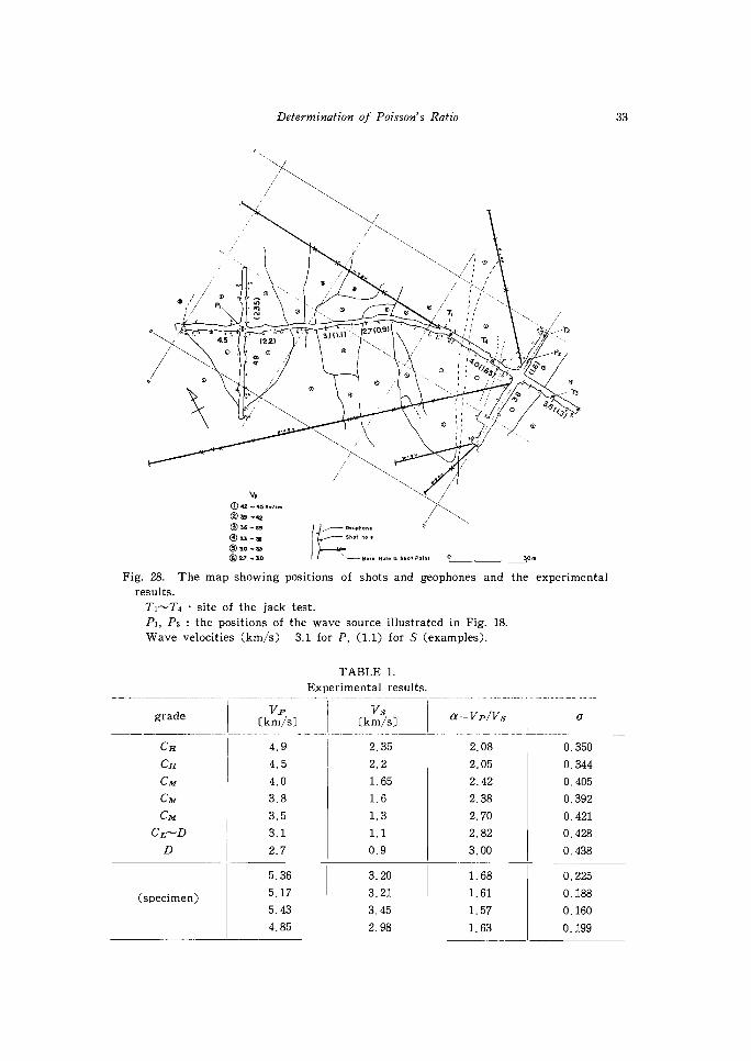
The most interesting problem for the author is the relation between a and V. This relation is demonstrated on Fig. 29, which shows clearly such a

32C. KITSUNEZAKI

MS . 0•- — 40— •

. + • .

P • S

• S S

•

V. •

_ 30—74‘.‘3 . , 4� , \7

Fig. 26. Travel time0 curve for P and S •. 'I

wave (spread : Ai -20: - +- Bi line) and the

structures correspon- /eo•

,

ding for them./ P,N4.1•\

P

(boundary ; — for 10_ 3b _ P, --- for S)/ ----- 3.e ...: . .

/ \ /.1----_____ ,

3p

0 Ai 3 5 6 7 6 9 lb II 12 0 3.0 ( 1.1) Bi

— — — — — —

3.8 (1.6 )

0I1Om—Jo

rns 50 -

• •

-1\ /--- \ P S/A7 S.

40-.

/,(P S•

,...'\

5

c'---

,--------o,

N Fig. 27. Travel time 30 7 'v

curve for P and SN . z wave (spread : C2 —

Z> E1 line) and the structures correspon- 20N\ 'V.b

ding for them.,' ounfor —P „

N

P--- -- 'N. (boundary ;— f-...,, ------x .___ P) x x.____,->"-----'

10 ----- - ---__•;->„. .... ___ 5 -•-1--- 40 •1

•—:::"-_-Hy21'`,,, ,. ..,,,, •' X-. '''-'--. - ---- -% 0. ,------ -5 ----*= .....____ 08 10(--Is 120

2 4 5 62 .. 9 30E , C /

3.5(1.31 I 40(165)

lom 0----lorn

Determination of Poisson's Ratio 33

/ /

, , = / A, - 0 ,,,1

o •1 ° ' ' a ' - I / P' 2 ///eittb:/To \ /

/111.•.27 (091•';••'..o','0 I,/y

•,,,,-.2

.

/ 0 , ! .1.! 0 , I ",,,, / :5!0.,, ! . Vii; . 2 m m

111‘

. ,

V, 0 42 -.4.51../..., 0 19 ̂ 42 P as -as ------

..:::::':ole (Da3-wi

®30-33 ® 27 -.30 N pore Hole II Shot Point 0 30rn

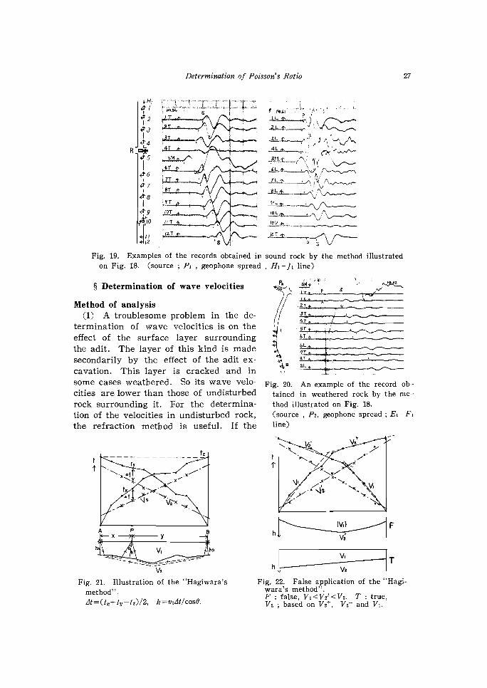
Fig. 28. The map showing positions of shots and geophones and the experimental results.

Ti-T4 • site of the jack test. PI, P2 : the positions of the wave source illustrated in Fig. 18.

Wave velocities (km/s) 3.1 for P, (1.1) for S (examples).

TABLE 1. Experimental results.

VpVs grade (km/s) (km/s) a=Vp/Vs (1

CH 4.9 2.35 2.08 0.350

CH 4.5 2.2 2.05 0.344

CM 4.0 1.65 2.42 0.405

CM 3.8 1.6 2.38 0.392

CM 3.5 1.3 2.70 0.421

CL---D 3.1 1.1 2.82 0.428

D 2.7 0.9 3.00 0.438

5.36 3.20 1.68 0.225

(specimen)5.17 3.21 1.61 0.188 5.43 3.45 1.57 0.160 4.85 2.98 1.63 0 .199

34 C. KITSUNEZAKI

tendency as a increases with decrease of V. Possible errors are thought to be about 3% for the P wave velocity and 6% for the S wave. Accordingly,

possible error of V,/Vs is nearly 10%. The relation between a and 171„, a -0 (V„), shall be assumed to be a linear equation. Its formula is deter-

mined by the means of the least square as follows,

a_=-V5,/Vs-=-0(V,)

= —0.49V„+4.34 (9)

For reference, the data obtained in X d' dye/cd situ on granite of other places are also X le kg/em'

plotted on Fig. 29. The supersonic test was also carried out for a few rock specimens obtained from bore50 holes in this field. They are thought to

give the values of the sound rock. 40 Ed .co rn

T.0 ›- 0 S 3.

3 • A U ^

• 2. L.,

• _ • •

*1 A, •10 • •••1-4--, e; ̂ e 2- •• • 4°•^•9

• 0731 0 • 02 3 4 5 km/sec

--> Vp

2 3 4 5 di.,•) measuNed value -p V, (Mm/sec) JenkTostlp mean value

Fig. 29. Plotting of the experimental re- Fig. 30. Variation of Young's modulus in sults.

Tsuruga . T ; in situ (Experimental for- granite. mula is determined for E : Young's modulus evaluated according

this.) to the experimental formula in Fig. S ; specimen (dry up in room t

emperature). 29. A, B including the surface d : the "conventional Young's modulus"

effect. (a=0 .25). Ushimado : U, Ikoma : I ; in situ.

Thus we have obtained the relation between V, and a . By Eqs. (3), (4) and (6) true Poisson's ratio and dynamic Young's modulus can be easily calculated. The latter is shown in Fig. 30.

Comparison between the dynamic method and the static

The result mentioned above shall be compared with the values by the jack test of which position is shown in Fig. 28. Definition of the Young's modulus in this case is illustrated in Fig. 31. The value of Young's modulus by this

Determination of Poisson's Ratio 35

40i— 6 (W.•P2) t

i ‘/ 171'' 'll I _,,,,

1k11,^rgli.;t''P _E.JI—Ch(R— P,) 2 a (^64-w) %11-,l' ‘

,

I.,

,„

/

_ E sffiill ----J.-

, //'16 —

2 0---;/ 0(r.3 '

gyp ) (W3,R) „Is7--='4-- 1. --—

0 0 mm V

\ i f / ---> W

Fig. 31. Illustration of the jack test and the definition of static Young's modulus Es.

W : displacement. V'=kV (k<1). P . load, a . radius of load plate.

TABLE 2. Results of the jack test.

E direction of No. sitenote (1041cg/cm2) pressure

1 T: 4.84 horizontal 2 T2 7.31 vertical 3 T3 0.46 vertical shear zone

4 T4 2.7 vertical

method is not practically affected by Poisson's ratio, because 72<1. This test was carried out by a company. The results are shown on Table 2.

The sites of the jack test are inhomogeneous, and their rock conditions are not the same. The velocity of the surface layer should be adopted as ones corresponding to the jack test, because its thickness h(3-5 m) is much larger than the radius of the load plate, a(15 cm). Evaluation of Young's modulus by the jack test is based on the assumption that a circular plate load is ap-

plied to the surface of semi-infinite elastic medium. Normal stress in the depth d decreases to less than 1/50 of that in the surface, when d/a>10"'. Accordingly, the effect of h to the evaluation of the Young's modulus can be

practically neglected, if h/a>10. The exact velocity of the jack test site, point by point, can not be evaluated, and it is not necessary for the present step of the discussion. We adopt 2.7 km/s as the mean velocity of P wave in the surface layer whose measured velocity is 2.3-3.0 km/sec. Density of the rocks determined by the laboratory experiment shows the values very near to 2.7 g/cm3. If we assume Eq. (9) can be also applied to the surface layer, Young's modulus is determined as 6.0 x 104 kg/cm2, which is shown in

36 C. KITSUNEZAKI

Fig. 30. Validity of this assumption was not completely assured in those sites, as mentioned later.

The value of the jack test No. 3 was obtained on the site particularily dif-ferent from the mean condition through the whole those sites. Therefore, this value should be rejected at the evaluation of the mean value of the jack tests. In this case it is determined as 4.9 x104 kg/cm2. Two Young's moduluses coincide each other sufficiently as such kind of discussion. If we assume Poisson's ratio as 0.25 conventionally and disregard velocity lowering in the surface layer (172,=3.7 km/sec. is adopted as the mean value), we obtain 29.5 x 104 kg/cm2 as Young's modulus. Such Young's modulus shall be especially called as "conventional dynamic modulus" in this paper. This is about six times the value by the jack test. That coincides approximately with the re-sults obtained by several authors.

According to this experiment, considerable discrepancy between the values by those two methods is not found. As shown in Fig. 30, Young's modulus is lowered to about a half of the conventional one, owing to adopt real Pois-son's ratio. Considering the velocity lowering in the surface layer, Young's modulus moreover falls to about half. Total lowering is about one fourth or one fifth.

Generalization of the experimental result

(1) As the author does not have enough data on many kinds of rock, he can not give the direct evidence to assure that the explanation mentioned above can be generalized to the problem on the discrepancy of the static and the dynamic modulus in all kinds of rock. However, a suggestion on this

problem is proposed by the following means. It shall be assumed that the static Young's modulus in situ is equivalent to

the dynamic Young's modulus modified by the effect of the variation of Pois-son's ratio and that of velocity lowering in the surface layer. The modulus defined by the above interpretation, Es'. is expressed as follows.

Es' =pk2V 1,2F(ak) (10)

ak=0(kV„)

where k is the effective reduction ratio of P wave velocity in the surface layer, compared with one of the surrounding rock (V2,). The function cb is assumed to be expressed by Eq. (9).

The "conventional dynamic Young's modulus" E/ is defined as follows .

=pV„2F(1 .73) (11)

Vp=1.73 corresponds to a=0.25. k =0 .75 is thought to be reasonable in com-mon conditions as the first approximation , as known from the examples in Table 3, though the value of k is affected by state and kind of rocks.

The relation between Es' and E/ can be directly determined from Fig . 30. It is demonstrated in Fig. 32.

The relation between Young's modulus by the jack test (Es) and one by the seismic method ("conventional modulus" Ea) was investigated by T. Onodera2) . The curve (Es) shown in Fig. 32 was given by him as the representative

Determination of Poisson's Ratio 37

TABLE 3. Velocity reduction due to the surface effect.

rock placeVpP(km/s) (km/s) ( =T71.p/V.p) (m)

4. 5 - 4. 9 3. 0 -3. 8 0.72* 3 - 5

granite Tsuruga 3. 5 - 4. 0 2. 3 - 3. 0 0.70* 2 - 5 3.5 2.6 0.7A

4.7 3.9 0.83 2 - 4

granite Ikoma 5. 2 - 5. 3 (5. 2- 5. 3) (1) 0 3.4 1.3 0.38 1 - 2

slate Shiroyama 4.2 1.7 0.40 1 - 3 4.4 1.9 0.43 1 - 4

V p : velocity (P) undisturbed by the surface effect. Tilp: velocity (P) of the surface layer.

h : thickness of the surface layer. : ratio for the:mean velocities.

xlekgk

Es 3•

Ei

2• '10

/ 010

A

C °. c,°

0 IC 20 30 40 50 -3.Ed• X104 k g/cm'

Fig. 32. Comparison of E's with Es. The curve Es and plotted points (measured values of Es) are cited from T.

Onodera's paper.

tendency of the relation, although the points were fairly scattered. E's in

case of k=0.75 well coincides with Es. In Onodera's relation the kind and the state of rocks were not classified, but they were mixed.

The problem to be studied is whether the relation a vs. V, in the surface

layer is the same as in the undistured rock surrounding it. Its direct measure-ment was difficult in the usual refraction line because of the irregularity of

rock condition in the surface layer and of its thinness. The velocities ob-tained in such a condition as shown in Fig. 11, give a suggestion for the

above problem. The velocity defined by the ratio between straight distance

of a shot point to a geophone and the travel time is strongly affected by the velocity of the surface layer, because the thickness of the surface layer,

3-5 m (effective value is twice this), is relatively large, compared with the

38 C. KITSUNEZAKI

straight distance, 20-30 m. The velocity ratios in this case are plotted in Fig. 29 with particularily distinguished marks. Their connections to the values of the "undisturbed rocks" in the same places are shown in this figure. In Group A, high velocity range, the relation of a vs. V, does not follow the

general tendency of the "undisturbed rock". a in the surface layer remains approximately as it is in the original undisturbed rock. In Group B, low velocity range, the tendentious discrepancy can not be found between them,

partly because of the wide scattering of points owing to the inhomogeneous condition that obstructs clear detection of the relation. The jack tests were carried out at this site.

Based on the preceding discussion, for reference, other possible Young's modulus of the surface layer is shown in Fig. 32. It is evaluated on the assump-tion as follows. a of the "undisturbed rock" is also conserved in one of the sur-face layer, and the coefficient of the velocity lowering in it, k, is 0.75. Hence,

Es" =k2V „2F (a) (12)

where a= 0(V„). '(V„) is assumed to be expressed by Eq. (9).

(2) Many experiments have confirmed that a in sound rocks have the values very near 1.73 (a=0.25). 0.25). Accordingly, if the experimental result of

granite can be generalized, a should be expressed by V„/V, instead of V„, where V, is the maximum velocity of P wave of the relevant rock (the velocity of the rock free from weathering effects). In Fig. 29 we take the value of V, which corresponds to a =1.73, as V,. It is 5.34 km/sec. Con-sidering the result of the supersonic measurement on the sound rock speci-mens in this field, this is a reasonable value. Hence, Eq. (9) is modified as follows.

a= – 2.6113+4.34 (13)

where 13 =V„/V,,.. By this relation F(a) can be expressed by 13.

F(a) =q((3) (14)

On the other hand, H. Masuda investigated the relation between the "con-ventional” dynamic Young's modulus (E',) by the seismic prospecting and the Young's modulus (ER). ER is the value which has been adopted by many

projectors for concrete dams according to their judgement. He proposed the following formula as the first approximation for this relation.

1V1(a)pV „2 (15) ER=,Eid- 2V

,2

where a=0.25. The Masuda's coefficient 18/2 was proposed for correction of the "conventional" dynamic Young's modulus so that it might be applied for engineering projects. In order to compare ER with the real dynamic Young's modulus E in Eq. (4), it suffices to compare fif(0.25)/2 with c(g). In Fig. 33 they are mutually compared.

There is not a considerable discrepancy between them in the region of j9< 0.8, which is the most common case.

From the preceding discussion it is suggested that there is not a considera-

Determination of Poisson's Ratio 39

ble discrepancy between the "true" dyamic

0, 4 \Young's modulus in situ (E) and the one used for engineering design (ER). The Masuda's coefficient will be replaced by

ythe ordinary effect of Poisson's ratio as 3 4the first approximation.

/

§ Conclusion 4/,

2 In situ ratio of P and S wave velocities (a) and Poisson's ratio (a) were measu-

50 red for various weathering states in 0 0.5 r granite. a approximately increases linear-

p

°ly with decrease of P wave velocity (V p). Fig. 33. Comparison between 5()3) and When the ratio of Vp to its maximum

"Masuda's formula". velocity (Vp.) decreases to 1/2, a increa- K - y= 0(3)• ses to about 3 (a =0.44).

M : y=0.417/3 ("Masuda's formula") Rocks in this field are thought to be M' : y=2>(0.4173. saturated by water . For the different

conditions and kinds of rocks, different results may be obtained. Further discussions of this is our future problem to be studied. If the present experi-ment can be extended to common rock, the discrepancy between the "conven-tional" dynamic Young's modulus and the static one in situ can be explained approximately by the effect caused by neglect of variation of Poisson's ratio in situ. Partly, that should also owe to the neglect (or incomplete correction) of the velocity lowering in the surface layer.

It is thought that expression of elasticity of rock by Poisson's ratio is not

practically adequate, because it approaches rapidly to the limit value 0.5 with a little increase of a. For example, a=3 is not an uncommon value, considering that a=5 is very common in sand and gravel"2). But

a =0.44 which corresponds to a =3, tends to give the impression that the state expressed by it is very liquid and not common. In consideration of the effect of Poisson's ratio, several investigators discussed only on the range very near to a =0.25. The author believes that a is more adequate than a for practical evaluation of the rock state.

Strictly speaking, this paper discusses only the comparison between the dynamic elastic properties in the particular range of stress and stress rate and the static Young's modulus defined according to particular engineering consideration. It is obvious that rock properties in situ are not completely elastic, but rather viscoelastic and plastic or more complex. According to the author's belief, only what cannot be explained by complete elastic treatment should be discussed in connection with inelastic properties of rock.

Acknowledgement

The author wishes to thank Prof. K. Sassa, who stressed the necessity of the study on the true value of Poisson's ratio and its applications to many

practical fields before popular attention began to be paid to those problems.

40 C. KITSUNEZAKI

The author also appreciates Prof. S. Yoshikawa's support for practice of the field experiment. Mr. N. Gotd, Mr. A. Kitazumi, Mr. T. Ikawa and Mr. I.

Nishizaki cooperated with the author in the field experiment. The author thanks them also.

Appendix Tanaka's Classification on the Feature of Rock")

Name Characteristics of the rock

The rock is very fresh, and the rock-forming minerals and grains are

A neither weathered nor deteriorated. The cracks and joints closely adhere

to one another. No trace of weathering is found along their surface.

The rock is solid. Neither crack (of even 1 mm.) nor joint is opened.

B They closely stick. But the rock forming minerals and grains are parti-

ally attacked by slight weathering and deterioration.

The rock forming minerals and grains excluding quartz are slightly soft-

CA by the weathering action. In general, the rock is stained by the

limonite, etc.

The rock forming minerals and grains excluding quartz are a little soft-

CA/ened by the weathering action. If it is struck, it peels off along the joints or cracks. On the broken off surface, the thin layer of red and,

or brown clay materials exist.

The rock forming minerals and grains excluding quartz are fairly soft-

ened by the weathering action. If it is slightly struck, it peels off along Ca the joints or cracks and breaks into little pieces.

Rock is much jointed and cracked. Among joints or cracks, the thin layer of red and, or brown clay materials exist.

(1) Affected by the weathering action, the rock-forming minerals and

grains are deteriorated, turned yellow-brown or brown, and the rock is remarkably softened. (the rock which looks like the weathered rock to

anybody)

D (2) On the rock-bed, there is found a developement of opened large cracks or joints. The rock-bed is subsequently divided into several

lumps. Though each rock lump is sound, the opened cracks or joints

can inhale the smoke, or the fire of handlamp.

(3) In addition, the fine roots of trees penetrate into the joint or crack

surface of the rock-bed.

(After Tanaka's paper)

References

1) Masuda, H. : Geophysical Exploration of the Dam Foundation, Butsuritanko (Geo-

physical Exploration), 13, 1960, pp. 25-35 (in Japanese). 2) Onodera, T. : General Note on the Geophysical Prospecting in the Construction

Ministry, Butsuritanko, 13, 1960, pp. 65-72 (in Japanese). 3) Jad, W. R. : Rock Stress, Rock Mechanics, and Research, State of the Stress in the

Determination of Poisson's Ratio 41

Earth Crust (International Conference held at Santa Monica, California, June, 1963),

pp. 5-54, Elsevier, New York. 4) Wantland, D.: Geophysical Measurement of Rock Properties in Situ, do., pp. 409-450. 5) Love, A. E. H. : A Treatise on the Mathematical Theory of Elasticity, p. 103, p.

297, Dover, New York. 6) Kusakabe, S. : A Keinetic Measurement of the Modulus of Elasticity for 158 Speci-

mens of Rocks, and a Note on the Relation between the Keinetic and Static Moduli, Pub. E. I. C. No. 22, 1906, B, pp. 27-49.

7) Kitsunezaki, C. : Study of High Frequency Seismic Prospecting (1), Butsuritanko, 13, 1960, pp. 102-107, pp. 137-146 (in Japanese).

8) Kitsunezaki, C. • High Frequency Seismic Prospecting, Geophys. Papers Dedicated to Professor Kenzo Sassa, pp. 179-185.

9) Hagiwara, T. • Butsuritanko, Asakura-shoten, Tokyo, 1951, p. 23. 10) White, J. E. . Seismic Waves, McGraw-Hill, New York, 1965, p. 214. 11) Yoshikawa, S., Shima, M. and Gotd, N. : On the Seismic Prospecting at the Area

Damaged by Niigata Earthquake, Disaster Prevention Res. Inst. Annuals, No. 8. 1965, pp. 19-34.

12) White, J. E. and Sengbush, R. L. : Velocity Measurements in Near-surface Forma- tions, Geophysics, Vol. 18, 1953, pp. 54-69.

13) Terzaghi, K. : Theoretical Soil Mechanics, John Wiley and Sons Inc., New York, p. 489.

14) Tanaka, H. : Geology of the Dam and the Treatment of its Foundation, Technical Report (Central Res. Inst. of Electric Power Industry) C-6203, 1963, p. 25.