In Search of Lost TimeA computational model of the representations and dynamics

of episodic memory

by

Yan Wu

A thesispresented to the University of Waterloo

in fulfillment of thethesis requirement for the degree of

Master of Applied Sciencein

Systems Design Engineering

Waterloo, Ontario, Canada, 2012

c© Yan Wu 2012

I hereby declare that I am the sole author of this thesis. This is a true copy of the thesis,including any required final revisions, as accepted by my examiners.

I understand that my thesis may be made electronically available to the public.

ii

Abstract

In Marcel Proust’s most famous novel, In Search of Lost Time, a Madeleine cake elicitedin him a nostalgic memory of Combray. Here we present a computational hypothesis ofhow such an episodic memory is represented in a brain area called the hippocampus, andhow the dynamics of the hippocampus allow the storage and recall of such past events.Using the Neural Engineering Framework (NEF), we show how different aspects of anevent, after compression, are represented together by hippocampal neurons as a vectorin a high dimensional memory space. Single neuron simulation results using this repre-sentation scheme match well with the observation that hippocampal neurons are tuned toboth spatial and non-spatial inputs. We then show that sequences of events representedby high dimensional vectors can be stored as episodic memories in a recurrent neuralnetwork (RNN) which is structurally similar to the hippocampus. We use a state-of-the-art Hessian-Free optimization algorithm to efficiently train this RNN. At the behaviourallevel we also show that, consistent with T-maze experiments on rodents, the storage andretrieval of past experiences facilitate subsequent decision-making tasks.

iii

Acknowledgments

First of all, I would like to thank my supervisors, Chris Eliasmith and Matthijs van derMeer, whose enthusiasm and wisdom make my studies a enjoyable experience, to whoseenormous support, within and beyond this thesis, I am deeply indebted. In addition, Iappreciate the discussion with James Martens. Without his generous suggestions, myimplementation of the Hessian-Free algorithm would not be so smooth. I would alsolike to thank my reader, Paul Fieguth, for his detailed and helpful comments. Specialthanks to Jane Russwurm, who warmly helps me with my English writing and proofreadpart of this thesis. Many thanks also go to colleagues in the Computational NeuroscienceResearch Group and the van der Meer Lab, especially to Xuan Choo, who helps me everytime when I have problems with my computer, Terry Stewart, who patiently answers allmy questions about the NEF, Rob Corss and Sushant Malhotra, who explain animalexperiments to me in intuitive and interesting ways.

iv

Dedication

This thesis is dedicated to my parents: Xiao Chunling and Wu Huabin. My gratitude tothem is far beyond any word in the “acknowledgement” part could express.

v

Table of Contents

List of Tables viii

List of Figures ix

1 Introduction 1

2 Background 32.1 Anatomy of the hippocampus . . . . . . . . . . . . . . . . . . . . . . . 32.2 Hippocampal cells . . . . . . . . . . . . . . . . . . . . . . . . . . . . 42.3 Remapping . . . . . . . . . . . . . . . . . . . . . . . . . . . . . . . . 72.4 Forward replay . . . . . . . . . . . . . . . . . . . . . . . . . . . . . . 82.5 Reverse replay . . . . . . . . . . . . . . . . . . . . . . . . . . . . . . . 9

3 Multi-dimensional neural representations 123.1 How spiking neurons represent vectors . . . . . . . . . . . . . . . . . . 123.2 Spatial representation . . . . . . . . . . . . . . . . . . . . . . . . . . . 15

3.2.1 Fourier basis and grid cells . . . . . . . . . . . . . . . . . . . . 183.3 Temporal representation . . . . . . . . . . . . . . . . . . . . . . . . . 203.4 Combining multi-modal representations . . . . . . . . . . . . . . . . . 233.5 Simulations of Remapping . . . . . . . . . . . . . . . . . . . . . . . . 25

3.5.1 Rate modulation . . . . . . . . . . . . . . . . . . . . . . . . . 253.5.2 Place field shifting . . . . . . . . . . . . . . . . . . . . . . . . 26

4 Hippocampal replay 284.1 The hippocampus as an information processing system . . . . . . . . . 284.2 Training the RNN . . . . . . . . . . . . . . . . . . . . . . . . . . . . . 294.3 Simulations of forward replay . . . . . . . . . . . . . . . . . . . . . . 304.4 Simulations of reverse replay . . . . . . . . . . . . . . . . . . . . . . . 344.5 Biased Initial Parameters and Oscillations . . . . . . . . . . . . . . . . 38

5 Discussion 425.1 The hippocampus and the neocortex . . . . . . . . . . . . . . . . . . . 425.2 The hippocampus and reinforcement learning . . . . . . . . . . . . . . 435.3 Comparison with other models . . . . . . . . . . . . . . . . . . . . . . 44

6 Conclusions 46

vi

Appendix 48

A Quadratic functions 49

B Back-propagation in NEF 51B.1 Notations . . . . . . . . . . . . . . . . . . . . . . . . . . . . . . . . . 51B.2 The Back-propagation Algorithm . . . . . . . . . . . . . . . . . . . . . 53B.3 Learning Rules . . . . . . . . . . . . . . . . . . . . . . . . . . . . . . 55B.4 Extension . . . . . . . . . . . . . . . . . . . . . . . . . . . . . . . . . 55

C Conjugate Gradients 56C.1 Linear conjugate gradient methods . . . . . . . . . . . . . . . . . . . . 56

C.1.1 Line search . . . . . . . . . . . . . . . . . . . . . . . . . . . . 57C.1.2 Conjugate directions . . . . . . . . . . . . . . . . . . . . . . . 57

C.1.2.1 Search directions are linearly independent . . . . . . 58C.1.2.2 Gradients are linearly independent . . . . . . . . . . 59

C.1.3 Constructing conjugate directions . . . . . . . . . . . . . . . . 60C.1.4 Convergence of conjugate gradients . . . . . . . . . . . . . . . 61C.1.5 The conjugate gradient algorithm . . . . . . . . . . . . . . . . 62

C.2 Non-linear Conjugate gradient methods . . . . . . . . . . . . . . . . . 63

D An efficient way of computing matrix-vector products 64

E Hessian-Free Optimization 66E.1 Overview . . . . . . . . . . . . . . . . . . . . . . . . . . . . . . . . . 66E.2 Positive semi-definite approximation . . . . . . . . . . . . . . . . . . . 66E.3 Optimization on quadratic approximation . . . . . . . . . . . . . . . . 68E.4 Modified Passes . . . . . . . . . . . . . . . . . . . . . . . . . . . . . . 69

E.4.1 Standard forward pass . . . . . . . . . . . . . . . . . . . . . . 70E.4.2 Standard backward pass . . . . . . . . . . . . . . . . . . . . . 70E.4.3 R-forward pass . . . . . . . . . . . . . . . . . . . . . . . . . . 71E.4.4 R-backward pass . . . . . . . . . . . . . . . . . . . . . . . . . 71E.4.5 Mini-batches . . . . . . . . . . . . . . . . . . . . . . . . . . . 71

E.5 The algorithm . . . . . . . . . . . . . . . . . . . . . . . . . . . . . . . 71

References 72

vii

List of Tables

4.1 Sequence learning performance and initial weights . . . . . . . . . . . 40

viii

List of Figures

2.1 The anatomical structure of the hippocampus . . . . . . . . . . . . . . 42.2 Spatial tuning of single hippocampal cells . . . . . . . . . . . . . . . . 52.3 Activity packet . . . . . . . . . . . . . . . . . . . . . . . . . . . . . . 52.4 Temporal tuning of hippocampal cells . . . . . . . . . . . . . . . . . . 62.5 Neural activity during the delay depends on both space and time . . . . 72.6 Remapping . . . . . . . . . . . . . . . . . . . . . . . . . . . . . . . . 82.7 The T-maze used in [85]. . . . . . . . . . . . . . . . . . . . . . . . . . 92.8 Decision-point forward replay . . . . . . . . . . . . . . . . . . . . . . 102.9 Reverse replay events . . . . . . . . . . . . . . . . . . . . . . . . . . . 11

3.1 1D tuning curves of LIF neurons . . . . . . . . . . . . . . . . . . . . . 143.2 The 2D tuning curve of a neuron . . . . . . . . . . . . . . . . . . . . . 143.3 The PSC in the frequency and temporal domains . . . . . . . . . . . . 163.4 Population-temporal representation . . . . . . . . . . . . . . . . . . . . 163.5 Reconstruction of the Gaussian function . . . . . . . . . . . . . . . . . 173.6 Simulation of an activity packet . . . . . . . . . . . . . . . . . . . . . 193.7 The firing rate of a population compared with decoded location from the

same population . . . . . . . . . . . . . . . . . . . . . . . . . . . . . . 193.8 An example of a Fourier basis function. . . . . . . . . . . . . . . . . . 203.9 Grid patterns . . . . . . . . . . . . . . . . . . . . . . . . . . . . . . . 213.10 Tuning curves of “time cells” . . . . . . . . . . . . . . . . . . . . . . . 213.11 Examples of PCA basis . . . . . . . . . . . . . . . . . . . . . . . . . . 223.12 Magnitudes (singular values) of the principal components . . . . . . . . 223.13 Reconstructed temporal representation . . . . . . . . . . . . . . . . . . 233.14 Simulated hippocampal cells . . . . . . . . . . . . . . . . . . . . . . . 243.15 Representation errors . . . . . . . . . . . . . . . . . . . . . . . . . . . 253.16 Simulation of remapping . . . . . . . . . . . . . . . . . . . . . . . . . 27

4.1 A recurrent neural network . . . . . . . . . . . . . . . . . . . . . . . . 294.2 Long short-term memory . . . . . . . . . . . . . . . . . . . . . . . . . 314.3 Epochs required for for different numbers of sequences with the length

of 20 time steps. . . . . . . . . . . . . . . . . . . . . . . . . . . . . . 324.4 A sequence for forward replay . . . . . . . . . . . . . . . . . . . . . . 334.5 Input cues and output from the RNN . . . . . . . . . . . . . . . . . . . 334.6 Simulation of decision-point forward replay . . . . . . . . . . . . . . . 354.7 An example input sequence and its target for reverse replay . . . . . . . 36

ix

4.8 Simulation of reverse replay . . . . . . . . . . . . . . . . . . . . . . . 374.9 Simulation of reverse replay for long sequences . . . . . . . . . . . . . 374.10 Averaged reverse replay error for sequences with different lengths . . . 384.11 Temporal oscillation patterns in the Hidden Layer of RNNs . . . . . . . 394.12 Hidden unit states can distinguish novel sequences . . . . . . . . . . . 41

B.1 A toy neural network . . . . . . . . . . . . . . . . . . . . . . . . . . . 51B.2 The activation function G(J) of a LIF neuron and it’s approximated first-

order derivative G′(J)∗. . . . . . . . . . . . . . . . . . . . . . . . . . . 52

x

Chapter 1

Introduction

As one of the most investigated parts of the brain, the hippocampus has been intenselystudied in both animal and human experiments. Notably, two seminal observations ledto two different hypotheses about the hippocampus [70]. In the early 1970s, O’Keefeand Dostrovsky [62] discovered the famous place cells, neurons in the hippocampus thatfire selectively at specific locations. This discovery later inspired the theory that thehippocampus plays the role of a cognitive map [64], by which animals maintain maps ofenvironments. Earlier than that, one of the most famous neurosurgeies, complete removalof both hippocampi, had been performed on a patient called H.M.1 [78] in order to controlhis severe seizures. H.M. immediately lost his ability to recall any event that happenedafter the surgery that removed a large part of his hippocampus. H.M.’s misfortune madeimportant contributions in the development of the theory that the hippocampus supportsepisodic memory, through which certain experiences are stored in a declarable state.

The dichotomy between the hippcampus’ role as a cognitive map or a central playerin episodic memory is more likely to be a result of different experiments, rather thanreflective of differences in the hippocampus itself [14, 22]. For example, in a typicalrat experiment, where neural signals are recorded while a rat is running in a maze, loca-tion is one of the most important and easily observable measurements. For this reason,the theory of cognitive maps was first developed through rat experiments, based on thediscovery of spatially correlated neural firing patterns [62]. Conversely, restricted by ei-ther ethical concerns or the subject’s natural behaviours, primate experiments, especiallyhuman experiments, seldom involve controlled location change2. As a result, the studyof spatial behaviors in primate experiments is severely limited. However, higher levelmemory tasks such as episodic recall are more often performed [81], resulting in thedevelopment of a theory of episodic memory in the context of primate experiments [84].

With the development of experimental techniques, however, more recent evidencefrom rat and primate experiments suggests an intimate relationship between cognitivemaps and episodic memory. For instance, recent data show that rat hippocampal cellsencode both spatial and non-spatial variables [20, 53, 54, 60, 66], in favor of multi-modal representations in a memory space [22]. Moreover, the reactivation of hippocam-

1His real name is Henry Gustav Molaison.2However, more recent experiments using virtual reality also found place cells in human

hippocampus[23]

1

pal cells’ spatially correlated patterns, or replay, is believed to be the neural correlateof the retrieval of episodic memory [13, 17, 29, 86, 92]. In addition, neural activitiesresembling one of the signature features of cognitive maps, remapping, in which the se-lective firing patterns of hippocampal cells are re-organized when an animal is exposedto a different environment, were also observed in the primate hippocampus [43].

Such converging experimental results motivate researchers to combine the two hy-pothesized roles of the hippocampus. In this thesis, we first introduce how the hip-pocampus can represent multi-modal information through vectors in a multi-dimensionalmemory space. Under this scheme, the cognitive map and episodic memory theory areunified naturally at the representation level. Further, we demonstrate how sequencesof vectors can be stored and retrieved in recurrent neural networks (RNNs) structurallysimilar to the hippocampus, resembling the storage and retrieval of episodic memory.Combining vector representations and temporal sequence learning, we simulated bothforward [85] and reverse replay [29] observed in rodent experiments. From a computa-tional perspective, our model supports the previously hypothesized role of awake replayin reinforcement learning [13, 29, 45]. Based on the simulation results, we propose an ex-perimentally testable prediction that forward and reverse replay rely on synaptic changeand persistent neural activity respectively.

2

Chapter 2

Background

Supported by a massive amount of experimental data from both humans and animals(e.g., [3, 6, 9, 12, 14]), the hippocampus is considered the as the place where episodicmemory, the memory of sequential events, is encoded. However, how episodic memoryis stored and retrieved in the hippocampus is still unclear, despite the existence of varioustheories (e.g., [9, 12, 14, 37, 84]). In this chapter, we start our investigation of how thehippocampus supports episodic memory by reviewing essential background materials.

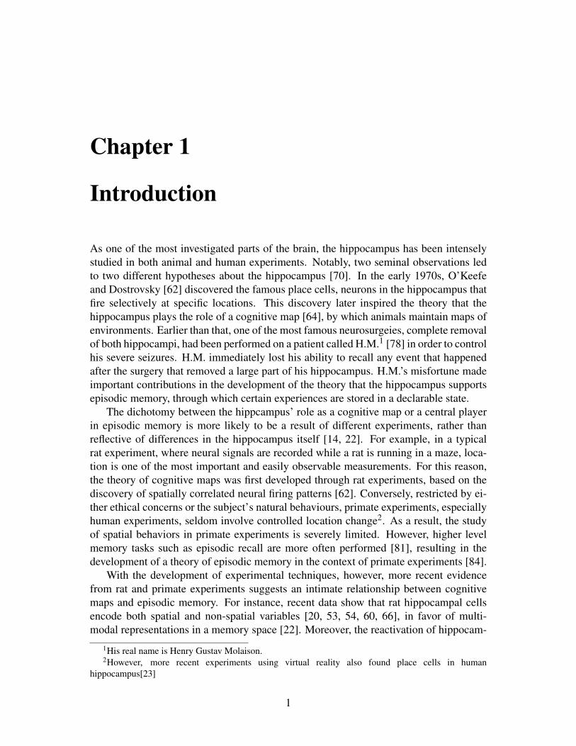
2.1 Anatomy of the hippocampusThe hippocampus is part of the forebrain, sitting beneath the neocortex. Figure 2.1 il-lustrates the anatomical structure of a rat’s hippocampus. It is characterized by feedbackloops at different levels: the local recurrent connections at the CA31 and the global feed-back connections passing through all components of the hippocampal formation (EC→DG→ CA1→ CA3→ Subiculum→ EC) [4].

The hippocampus receives information from different sources mainly through the en-torhinal cortex (EC), which closely interacts with a diverse range of other cortical areas,permitting the encoding of multi-modal information in episodic memory. The dentategyrus (DG) is one of the only two places in the brain where adult neurogenesis happens[1] (the other is the olfactory bulb). The EC is connected to DG through the perforantpathway, and it sends direct projections to the CA3, CA1 and the subiculum. The DGgranule cells send their output to the pyramidal cells in the CA3 through mossy fibers,whose strong connections enable the CA3 neurons to be activated by very sparse activ-ities in the DG. Compared with the typical mostly-local connections in the neocortex,the dense recurrent connections across the whole CA3 region are unique in the brain,allowing globally synchronized activities of the CA3 pyramidal cells. Pyramidal cells inthe CA1 receive input from the CA3 through Schaffer collaterals. Traditionally, the DGand the CA are considered to be the central part of the hippocampus, called the “hip-pocampus proper”; the hippocampus proper and its surrounding area, including the EC,the subiculum, and the parasubiculum, are together called the hippocampal formation2.

1CA is the acronym for cornu ammonis, or Ammon’s horns. However, this full name is seldom used.2However, there are other opinions concerning which parts should be considered as the hippocampal

3

(a) (b)

Figure 2.1: The anatomical structure of the hippocampus and its cartoon illustration.Figure (a) is a diagram of a rat’s hippocampus, showing the anatomical structure of thehippocampal formation (EC: entorhinal cortex, DG: dentate gyrus, Sub: subiculum) [4].(b) illustrates main parts of the hippocampal formation and connections between them.

2.2 Hippocampal cellsThe most famous neurons in the hippocampus are probably the place cells, which areknown for their selective spatial firing patterns. Place cells were first discovered in theCA1 region in the hippocampus, and later were also found in the CA3, the DG andthe subiculumn [4, 62]. Initially, place cells were only thought to support the neuralrepresentation of the spatial properties of the environment, forming cognitive maps [63]for spatially related behaviours such as navigation. A place cell fires only when therat is close enough to that cell’s place field3. Figure 2.2 illustrates the place fields ofsome place cells. The contours of these place fields can be approximated by Gaussianfunctions. When the firing of place cells are arranged topographically according to theirplace fields (so that place cells representing similar places are together), a populationlevel Gaussian-shaped pattern, the activity packet, can be observed (figure 2.3). Arisingfrom the Gaussian tuning curves of individual hippocampal cells, activity packets can beused to estimate the location of the animal. For example, the activity packet in figure 2.3indicates that the rat is at the center of an environment.

More recently, temporally selective activities of the hippocampal cells were observedat different laboratories, from recordings during delay periods of tasks [66, 53]. Specif-ically, they show that strong temporal modulation in their recoded hippocampal cellsis preserved even after statistically removing the influence of location and behaviour.For this reason, they call these cells “time cells”4to contrast with the famous place cells

formation [4].3Exceptions are that place cells also fire in hippocampal replay events, which may happen when the

rat is in REM sleep, slow wave sleep or staying stationary. Besides, a place cell may have multiple placefields [27].

4Although the concept of “time cells” may be controversial, for simplicity, later we use neurons “rep-

4

Figure 2.2: Spatial tuning of single hippocampal cells [91]. The color map, in whichred represents high firing rates and blue represents low firing rates, showing single cellrecording from hippocampal neurons in the CA1 region of the hippocampus when arat was freely foraging in an open field. In this specific environment, while some cellsshowed clear location selective firing, other cells either fire thoughout the whole envi-ronment (e.g., upper-right corner) or keep silent all the time (e.g., upper-left corner).

Figure 2.3: Activity packet visualizing the firing rate of a population of place cells [75].Neurons are arranged according to their place fields, so that their positions on the figureare roughly the same as their preferred locations in the environment. In this figure,neurons at the center fire most strongly, implying the rat was near the center of the testingenvironment.

5

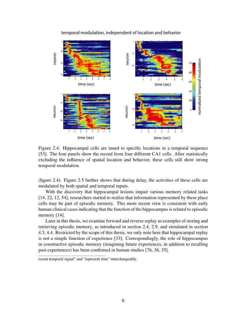
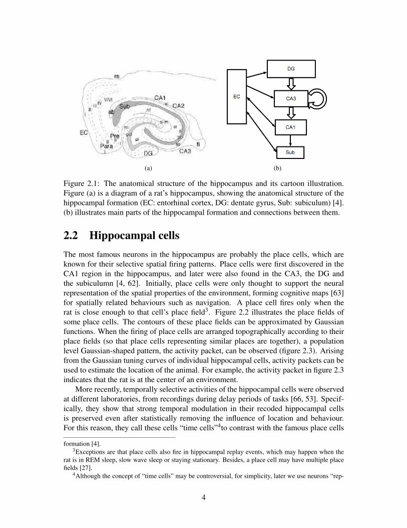
Figure 2.4: Hippocampal cells are tuned to specific locations in a temporal sequence[53]. The four panels show the record from four different CA1 cells. After statisticallyexcluding the influence of spatial location and behavior, these cells still show strongtemporal modulation.

(figure 2.4). Figure 2.5 further shows that during delay, the activities of these cells aremodulated by both spatial and temporal inputs.

With the discovery that hippocampal lesions impair various memory related tasks[14, 22, 12, 54], researchers started to realize that information represented by these placecells may be part of episodic memory. This more recent view is consistent with earlyhuman clinical cases indicating that the function of the hippocampus is related to episodicmemory [14].

Later in this thesis, we examine forward and reverse replay as examples of storing andretrieving episodic memory, as introduced in section 2.4, 2.9, and simulated in section4.3, 4.4. Restricted by the scope of this thesis, we only note here that hippocampal replayis not a simple function of experience [33]. Correspondingly, the role of hippocampusin constructive episodic memory (imagining future experiences, in addition to recallingpast experiences) has been confirmed in human studies [76, 36, 35].

resent temporal signal” and “represent time” interchangeably.

6

Figure 2.5: Neural activity during the delay depends on both space and time. In theexperiment in [53], a delay is introduced between two phases. The spatial firing ratemaps for 2 hippocampal cells are shown. For each cell the top map is for the entire delay,and maps below focus on each individual second of the delay.

2.3 RemappingIn order to support episodic memory, a problem faced by the hippocampus is the pos-sible ambiguity in representation. An example commonly used by researchers studyingepisodic memory is the scenario of parking a car: although both the car and the parkinglot are the same each day, ones needs to remember today’s parking location (or path)as distinguished from that of yesterday or before. In this example, the time (today orother days) provides the context based on which different memories of parking can beretrieved. In rodent maze experiments, this problem is usually presented as requiring arat to behavior differently based on different context [15].

Given the presence of ambiguity in various tasks, it is not surprising that the brain, es-pecially the hippocampus, has different ways to disambiguate inputs at the neural level.First, the Gaussian tuning curve (figure 2.2) leads to sparse firing patterns (figure 2.3,where only cells proximal to the center are firing). Sparse firing patterns maintain lowinterference because of low overlapping between different patterns. Although the func-tionality of neurogenesis in the DG is still not entirely clear, it is believed to facilitate theorthogonalization of input into the hippocampus [1, 7, 83]. Another way to disambiguateis remapping, as if a animal uses different maps for different contexts.

Two kinds of remapping are observed in rodent experiments5: rate remapping andglobal remapping [15]. In rate remapping, a hippocampal neuron fires differentiallyin different environments only through its firing rate changing. In global remapping, inaddition to the change of firing rate, a neuron’s place field may either change or disappearin different environments (figure 2.6). Through these changes of spatial correlated firing,different “maps” are formed for different environments. For example, the same locationat the center of two different environments will be represented by different neurons.

5Phenomena similar to remapping are also observed in human fMRI studies [9].

7

Figure 2.6: Rate remapping (left) and global remapping (right) [15]. The color map isused to indicate firing rate as with previous figures. On each side, the first column illus-trates the firing of neurons in one environment, while as the last two columns illustratethat in the other environment. The mapping from firing rates to colors are the same in thefirst two columns, but are rescaled in the third column. For rate remapping, the activity ofneurons looks the same after rescaling, indicating the firing in two different environmentsis only distinguished by firing rates. On the contrary, for global remapping, the neuralactivity is different even after rescaling the color map, showing the preferred locations ofthese cells are also changed.

Similarly, traces sharing similar relative potions in two environments will be representedby distinct neurons. Thus ambiguity cased by sharing representations (sharing “maps”)can be largely reduced.

2.4 Forward replayWe mainly consider the forward replay observed in rodent T-maze experiment [46, 86]6.A T-maze (figure 2.7) has three connected arms (left, central, right), with possible feedersproviding food or drink as reward at the left or right arms. When a rat is at the central armof the T-maze, it needs to choose which side to go to, as only one arm of the T-maze givesthe desired reward. The location right before the intersection of the “T” point (indicatedby the white circle in figure 2.8) is called the decision point. At early learning stages ofthe T-maze experiments, the rat pauses at the decision point before proceeding, as if it ispondering which side to go to [85].

6In this thesis, we use the term “forward replay” and “sweep” interchangeably to refer to the reactiva-tion of hippocampal neural activities at the decision point, although the exact relationship between theseterms are not entirely clear in neuroscience literature.

8

Figure 2.7: The T-maze used in [85].

This intuitive hypothesis is supported by multi-cell recordings from the rat hippocam-pus, which indicates that previously visited routes including both arms are replayed at thedecision point through the reactivation of hippocampal cells (figure 2.8). Interestingly, atthe about same time as the replay (or “sweep”), cells in ventral striatum that are activatedwhen reward is presented are also firing, implying that forward replay may be linked tothe evaluation of future outcome[86].

2.5 Reverse replayAs suggested by its name, reverse replay also involves the reactivation of past neuralactivities representing past experiences, however, in a reversed order. Although the re-played sequences can be either remote [17, 33] or recent in the past [29], in this thesiswe mainly consider the reverse replay of recent experience7. This kind of replay hap-pens immediately after a rat reaches a goal or obtains a reward [29]. For reasons we willdiscuss in more detail in section 4.4, remote reverse replay may be similar to forwardreplay, while as the reverse replay of recent experience is likely to be based on a differentcomputational mechanism. Figure 2.9 shows the reverse replay recorded during a singlelap on a linear track.

7Therefore, without specification, later in this thesis “reverse replay” means the replay of recent expe-rience.

9

Figure 2.8: Replay at the T-maze decision point [86]. Each sub-plot shows decoded rep-resentation at different time during the rat’s being at the decision point (white circle); thecolor code indicates the probabilities of the represented location, where blue to red meanslow to high probabilities. From the decoded spatial representation in these sub-plots, al-though the rat was keeping still, the locations represented in its hippocampus driftedtowards each possible future direction, indicating the replay of previous experiences atdifferent arms.

10

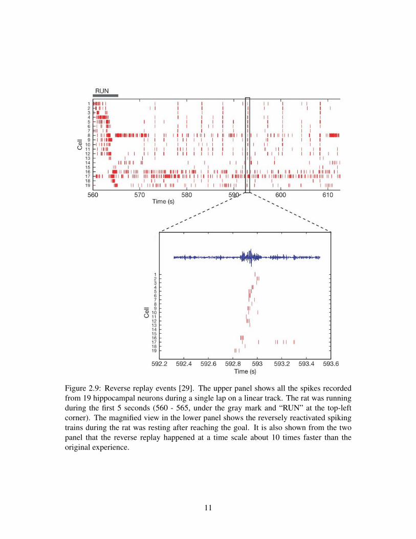
Figure 2.9: Reverse replay events [29]. The upper panel shows all the spikes recordedfrom 19 hippocampal neurons during a single lap on a linear track. The rat was runningduring the first 5 seconds (560 - 565, under the gray mark and “RUN” at the top-leftcorner). The magnified view in the lower panel shows the reversely reactivated spikingtrains during the rat was resting after reaching the goal. It is also shown from the twopanel that the reverse replay happened at a time scale about 10 times faster than theoriginal experience.

11

Chapter 3

Multi-dimensional neuralrepresentations

We can understand episodic memory as temporal sequences in a high dimensional mem-ory space, in which different kinds of (multi-modal) information are bound togetherthrough experiences [22]. Mathematically, temporal sequences can be represented assequences of vectors in this memory space. In this chapter, we introduce how vectorscan be represented in spiking neurons and how we can use such vectors to representvariables potentially forming episodic memory. In the next chapter, we describe howsequences of these vector can be remembered as traces of episodic memory.

While a vector may have multiple elements, or multiple dimensions, we can dividea vector into subgroups that represent different information from different sources. Forexample, a six dimensional vector, t = (1,0,3,7,5,9)>, can devote its first two dimen-sions to represent hours, the middle two dimensions to represent minutes and the lasttwo dimensions to represent seconds. Together, t represents a specific time. In a similarmanner, for the vector v used in our hippocampal representation, we can divide it intodimensions representing space, dimensions representing task, etc.

3.1 How spiking neurons represent vectorsThe Neural Engineering Framework (NEF) [25] provides a theoretical framework forcharacterizing neural representations, neural transformation and neural dynamics acrossdifferent levels of description. This section introduces the first principle in the NEF, neu-ral representation, by which vectors can be represented in biologically plausible spikingneurons. Although the NEF supports simulation of neurons with different levels of phys-iological details, for simplicity, this thesis uses leaky-integrated-and-fire (LIF) neurons[25].

The sub-threshold dynamics of a LIF neuron is described by the differential equation:

dVdt

=− 1τRC (V − J ·R) (3.1)

where both τRC, the membrane time constant, and R, the leak resistance, are parame-

12

ters. This equation describes how the membrane potential V of a LIF neuron changewith time t given the input current J when V is below a threshold Vthreshold . Once themembrane potential reaches a threshold Vthreshold (at which time the current also reachesits threshold Jthreshold), the LIF neuron generates a spike. A spike, or action potential,is a transient and dramatic increase of its membrane potential followed by a refractoryperiod. During the refractory period, the membrane potential keeps at a low level for ashort amount of time specified by the parameter τre f . When the input current is constant,we can analytically solve for the firing rates of a LIF neuron:

a(J) = G(J) =1

τre f − τRCln(1− JthresholdJ )

(3.2)

The NEF suggests that, for a given neuron, its input current is regulated by a vector x inits input space through

J = γ · (e · x)+b (3.3)

where e is the normalized unit encoder of this neuron, γ is gain factor, and b is the inputbias. The parameters γ , e, b as well as τRC and τre f together specify the tuning curve ofa LIF neuron, as a function of vector x in its input space. The encoder e is also calledthe preferred direction of a neuron, because for input vector x with fixed lengths, the dotproduct e · x reaches a maximum when x has the same direction as e, which in turn givesthe maximum firing rate (equation 3.3 and 3.2).

The tuning curve of 20 LIF neurons with one dimensional input is shown in figure3.1, and the tuning curve of a neuron with two dimensional input is shown in figure 3.2.Given a population of heterogeneous neurons, through activation functions defined byequation 3.2 and 3.3, a vector x can be encoded into the firing of these neurons. Sinceactivation functions are non-linear, this is a process of non-linear encoding.

The encoding process need to be paired with a corresponding decoding process thatreads out the encoded vector x. Given the complexity of possible non-linear decoding,the NEF suggests that linear decoding is a general and more biologically plausible mech-anism. With a decoder d for each neuron in a population, we can decode the estimationof x from the activity of this population:

x = ad (3.4)

For a population representing x in an input space S, equation 3.4 should give a goodestimation for all x in S. Therefore, we extend equation 3.4 for a set of representative1

samples in the input space S by substituting each lower case variable with capitalizedletters representing samples in the whole input space, giving a system of linear equations:

X = A>D (3.5)

Now each column represents one dimension of space S, and each row of X representsa sample in this space. Each column of A represents the firing rate of a neuron in this

1whether a set of sample is representative is determined by the space S. In general, more samples areneeded for higher dimensional spaces with more complex structure.

13

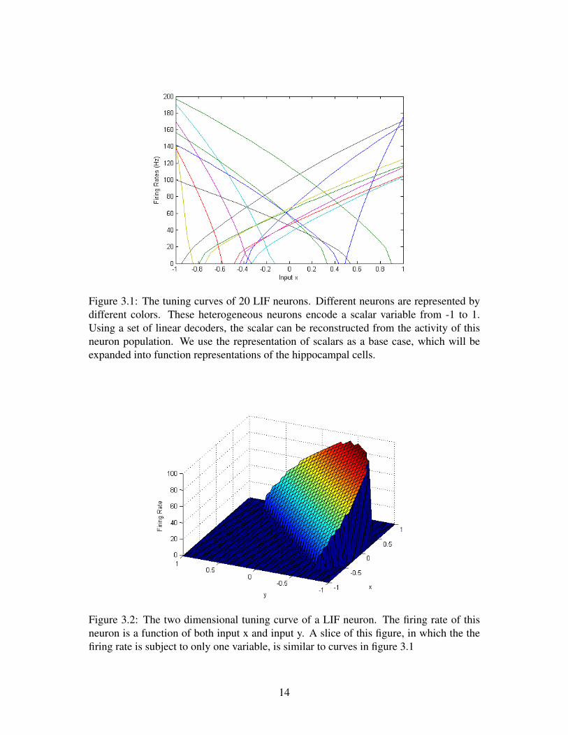
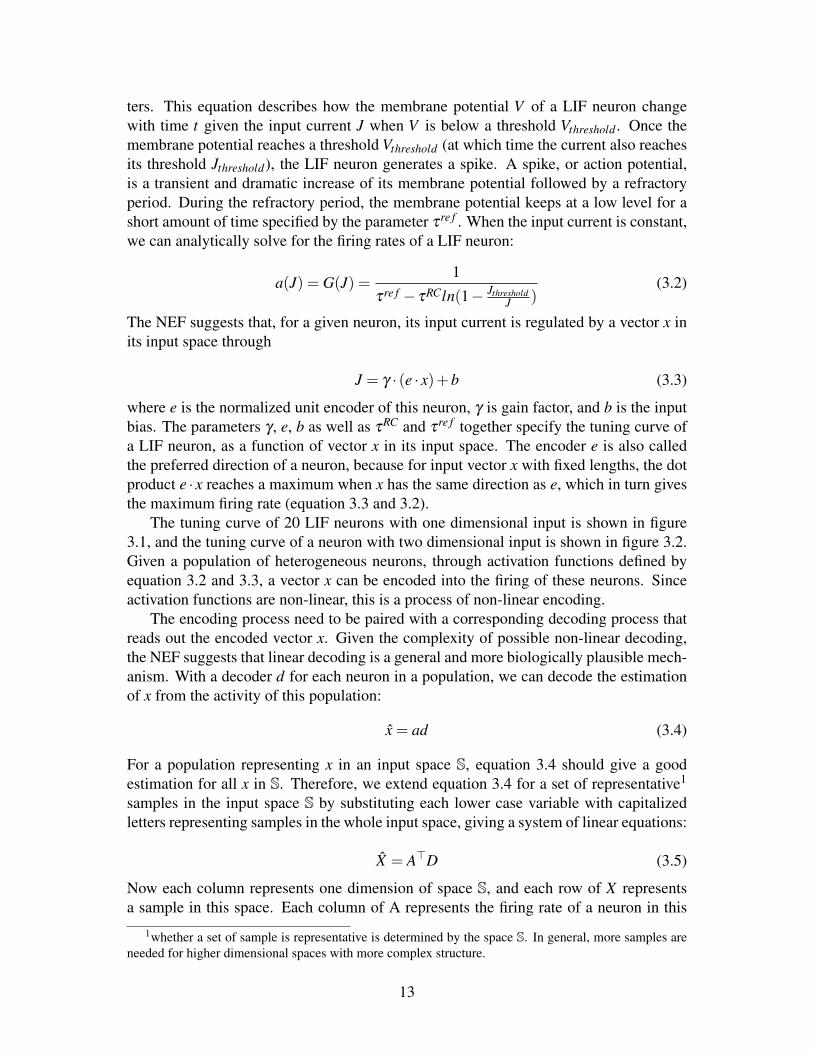
Figure 3.1: The tuning curves of 20 LIF neurons. Different neurons are represented bydifferent colors. These heterogeneous neurons encode a scalar variable from -1 to 1.Using a set of linear decoders, the scalar can be reconstructed from the activity of thisneuron population. We use the representation of scalars as a base case, which will beexpanded into function representations of the hippocampal cells.

Figure 3.2: The two dimensional tuning curve of a LIF neuron. The firing rate of thisneuron is a function of both input x and input y. A slice of this figure, in which the thefiring rate is subject to only one variable, is similar to curves in figure 3.1

14

population, while each row represents the activity of the population given one sampleinput. Similarly, each column of D represents the input dimension corresponding to X ,and each row of D represent the decoder for one neuron.

We can understand equation 3.5 as projecting vectors from the neural space, wherethe tuning curves of neurons serves as basis, back to the original Cartesian space. There-fore, finding the decoders is a regression problem and the decoders D can be solvedanalytically using the conventional normal equation:

D = (A> ·A)−1 ·A> ·X (3.6)

As one of the most well studied equations in numerical analysis, equation 3.6 can beevaluated efficiently through a singular value decomposition (SVD).

Now we turn to the temporal dynamics of LIF neurons by allowing the input currentto change. Although equation 3.2 is no longer true, the effect of spikes can still beaccumulated though the post-synaptic current (PSC):

hpsc(t) = e−t

τsyn (3.7)

As illustrated in figure 3.3, the PSC smooths the spikes; the smoothness is controlledby the parameter τsyn, the synaptic time constant. The PSC bridges rate coding andspike coding by providing a diminishing time window, in which the effect of spikesis accumulated as the strength of the current. Filtering a spike train by the PSC canrecover the original signal, albeit with additional errors introduced the the fluctuation ofthe spikes (figure 3.4). This filtering process can be embedded at the synapse as

dJPSC

dt=−τPSC

JPSC(3.8)

Thus, we have now established a representation scheme for spiking neurons. Ourway of deriving the optimal linear decoders supports the smooth transactions betweenrate coding and spike coding, two neural coding schemes that may not be fundamentallydifferent [25]. Nevertheless, supporting spikes makes our model easier to compare withexperimental data. For more detailed description, refer to [25].

In the context of episodic memory, for a population of neurons representing eventsin memory as vectors x, the input space S becomes the memory space. In the followingsections, we discuss properties of this memory space, and further characterize vectors inthis memory space.

3.2 Spatial representationUsing the vector representation scheme introduced in the last section, many variablescan be encoded and decoded in spiking neurons. However, more structured variablesare required to represent information essential in episodic memory, such as locations.This section extends the vector representation scheme by showing how more structuredfunctions can be represented. The basic idea of function representation in NEF is de-composition (dimension reduction) of discrete functions.

15

Figure 3.3: The PSC in the frequency and temporal domains. As we can see from thefrequency domain illustration, high frequency components are suppressed. Therefore,the PSC smooths spikes.

Figure 3.4: Estimation of the original signal. The estimation is obtained from filteringspikes generated by each LIF neuron in a population of 20 LIF neurons, then sum up thefiltered signals weighted by the decoders (equation 3.6). The fluctuation is introduced bythe spikes and the high-frequency components of the PSC.

16

(a) (b)

Figure 3.5: Reconstruction of the Gaussian function with different maximum frequencycomponents. (a) Reconstruction using components with a maximum frequency of 10 Hz.(b) Reconstruction with components with a maximum frequency of 3 Hz. Although (a) iscloser to the original Gaussian function, (b) also gives a reasonably good approximationfor our qualitative simulations.

Inspired by the Gaussian shaped spatial tuning curves of the hippocampal cells (sec-tion 2.2), Conklin and Eliasmith [16] simulated Gaussian firing patterns of place cellsfrom a population of neurons representing two dimensional Gaussian functions.

A Gaussian function (figure 3.5 (a))

f (x,y) = exp(−(x−µx)

2 +(y−µy)2

2σ2) (3.9)

can be discretized into a vector with a finite (large) number of dimensions. In order toguarantee an acceptable representation precision, the number of neurons in a populationusually increases as the number of dimensions represented increases.2 Therefore, di-mension reduction is required to represent functions in our vector representation scheme.For any function, one conventional way of performing dimension reduction is using theFourier transformation, decomposing the function into basis and coefficients

Fkl = ∑m

∑n

f (xm,yn) · e−2πi( kM m+ l

N n) (3.10)

where f ’s are values of the function in spatial domain and F’s are coefficients in fre-quency domain. Preserving a finite number of coefficients results in a reduced approxi-mation to the full Fourier space. Using the inverse Fourier transformation, we can restorethe spatial domain function from coefficients F’s and the oscillatory basis e2πi( k

M m+ lN n)

(e.g., figure 3.8)

fmn = ∑k

∑l

Fkl · e2πi( kM m+ l

N n) (3.11)

Recall that the Fourier transformation of a Gaussian function is still a Gaussian func-tion, so the coefficients of a Gaussian function diminish quickly as the frequency in-

2This statement is not strictly true, since different dimensions may be correlated.

17

creases. This property implies that we can discard high frequency components and stillmaintain a good representation of the Gaussian function. Figure 3.5 shows the recon-struction using components with frequencies less than 3Hz, compared with the recon-structed Gaussian function with more frequency components.

In general, function decomposition (not necessarily Fourier decomposition) providesa way to simplify the representation of an otherwise continuous space. This also simpli-fies the calculation of similarity between an input and the preferred direction vector ofa give neuron3. Mathematically, since the firing of a neuron is only affected by the dotproduct between its encoder and the input vector obtained from function decomposition,the basis is not directly involved in neural computation. Providing that the basis is cho-sen properly (i.e., it is able to give a good reconstruction of the original function) andthe coefficients are represented well, the firing pattern is only affected by the functionbeing represented. In fact, both a Fourier basis and a basis obtained from principal com-ponent analysis (PCA) can reproduce the same Gaussian firing pattern reported in [16].Although in theory PCA does a better job at dimension reduction, a Fourier basis maybe realized in the brain as the observed sub-threshold oscillations at different frequencies(this issue is further discussed in section 3.2.1).

Using this spatial representation scheme, an activity packet resembling that in figure2.3 is simulated in a population of 4,900 neurons (figure 3.6), where each neuron rep-resent a Gaussian function with width (δ in equation 3.9) 0.1, centralized at locationsevenly sampled in a 2D square. In order to illustrate the activity packet, these neuronsare organized topographically. Note neurons in this population are not interconnected, al-though they can be connected in the same way as in [16], forming an attractor. Althoughthe activity packet is able to indicate the location of the animal from the distribution ofneural activity (red areas in 3.7 a), using the full NEF neural representation gives a muchbetter estimations (3.7 b). With the multi-dimensional decoders, instead of estimatingthe compound information from the 1D firing rate only, different dimensions of the rep-resented vectors can be decoded separately. Therefore, the advantage of using neuralcoding is even more obvious with the presence of non-spatially encoded information andnoise.

3.2.1 Fourier basis and grid cellsAs a digression from the vector representations in episodic memory, here we brieflygive a justification of choosing the Fourier basis for function decomposition. A Fourierbasis function e2πi( k

M m+ lN n), which is sometimes written as sine and cosine functions, is

illustrated in figure 3.8. The interference of three such waves separated by 60 degreesproduces the hexagonal pattern reminding us the firing patterns of grid cells (figure 3.9).

Such an interference mechanism is used in various models of grid cells [11, 31, 80].Physiologically, the Fourier basis (waves) may be realized in neural networks as sub-threshold oscillations which are found in the hippocampal formation. More specifically,these oscillations may be originated from the intrinsic oscillations in the entorhinal cor-

3Therefore, although only vectors are represented by the neurons, we sometimes call it function repre-sentation in this situation

18

Figure 3.6: Simulation of an activity packet using 4900 LIF neurons arranged accordingto their place fields. Each cell represent a Gaussian function through their coefficientsobtained from Fourier decomposition. These Gaussian functions have with fixed width,sampled evenly from the 2D square. The two horizontal axes index each cell and thevertical axis is proportional to the firing rates.

(a) (b)

Figure 3.7: The firing rate of a population compared with decoded location from the samepopulation. Figure (a) is a top view of figure 3.6, indicating the firing rate of neurons inthis population. Figure (b) shows the decoded spatial representation using the optimallinear decoder. This 2D map is obtained from taking the dimensions representing spacefrom the decoded vector (equation 3.5) as coefficients and reconstructing the 2D surfacetogether with the Fourier basis. While it is possible to (roughly) determine the encodedlocation from the firing rates only (a), neural decoding give a much better estimation ofthe represented location (b).

19

Figure 3.8: An example of a Fourier basis function.

tex [31, 38]. The frequencies of these oscillation are proportional to the velocity of theanimal. Specifically, the direction information comes from the head direction cells inthe parahippocampus. These oscillations are summed, forming new sub-threshold os-cillation patterns like that in figure 3.9 A. When receiving spiking input with certainfrequencies, the grid cells are more likely to reach the threshold and fire when the sub-threshold oscillation near the peaks (places in figure 3.9 (a) where the color close tored). Thresholding the pattern in figure 3.9 (a) gives figure 3.9 (b) that is similar to theexperimentally observed grid firing patterns [30, 34].

Since both e−2πi( kM m+ l

N n) in equation 3.10 and e2πi( kM m+ l

N n) in equation 3.11 can berepresented as oscillations, the combination of them can form the hexagonal patterns ofthe grid cells. Given the fact that the entorhinal cortex, where these grid cells reside,serves as both input and (indirect) output of the hippocampus proper, our representationscheme is consistent with the view that the grid cells also support decoding of spatial in-formation, in addition to supporting encoding as an upstream input to the hippocampus4

[28].

3.3 Temporal representationIn order to form a unified and systematic representation scheme, we specify that hip-pocampal cells are also tuned to temporal sequences directly. This design choice doesn’tviolate the assumption that the “time cells” are resulted from intrinsic temporal dynamics[26, 66], since these temporal sequences can be generated internally from an integratorlike structure.

From a modeler’s view, by analogy to how space is represented, temporal signalscan be represented in our model as vectors obtained from decomposing one dimensional

4When grid cells are used as basis directly, the the linear relationship between basis and Gaussianfunctions is still held, although the coefficients for these basis are computed in a different way [80].

20

(a) (b)

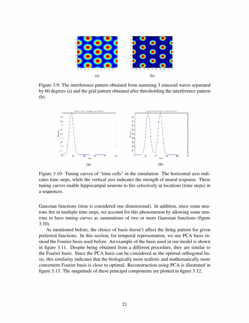
Figure 3.9: The interference pattern obtained from summing 3 sinusoid waves separatedby 60 degrees (a) and the grid pattern obtained after thresholding the interference pattern(b).

(a) (b)

Figure 3.10: Tuning curves of “time cells” in the simulation. The horizontal axis indi-cates time steps, while the vertical axis indicates the strength of neural response. Thesetuning curves enable hippocampal neurons to fire selectively at locations (time steps) ina sequences.

Gaussian functions (time is considered one dimensional). In addition, since some neu-rons fire in multiple time steps, we account for this phenomenon by allowing some neu-rons to have tuning curves as summations of two or more Gaussian functions (figure3.10).

As mentioned before, the choice of basis doesn’t affect the firing pattern for givenpreferred functions. In this section, for temporal representation, we use PCA basis in-stead the Fourier basis used before. An example of the basis used in our model is shownin figure 3.11. Despite being obtained from a different procedure, they are similar tothe Fourier basis. Since the PCA basis can be considered as the optimal orthogonal ba-sis, this similarity indicates that the biologically more realistic and mathematically moreconvenient Fourier basis is close to optimal. Reconstruction using PCA is illustrated infigure 3.13. The magnitude of these principal components are plotted in figure 3.12.

21

(a) (b)

(c) (d)

Figure 3.11: Examples of PCA basis. They may look like Fourier basis, but a closer lookat the horizontal lines (black dash lines) reveals that they are not. Therefore, the fourierbases are close to optimal.

Figure 3.12: Magnitudes (singular values) of the principal components. The red lineindicates the number of components used in our experiments.

22

Figure 3.13: Reconstructed temporal representation (a one dimensional Gaussian func-tion with mean at 100) from decoded coefficients (as vectors) and PCA basis. Due toboth the limited basis used and the induced noise, the reconstructed temporal represen-tation is not perfectly smooth. Nevertheless, the time step it represents (near 100), as isvery clear, as the position that gives the highest value.

3.4 Combining multi-modal representationsCombining vectors representing multi-modal information gives the multi-modal repre-sentations used in our hippocampus model. In addition to spatial and temporal inputsbeing represented in the way described in the previous two sections, other variables canbe represented either similarly through decomposition of functions or directly as vectors.

When a neuron is assigned a preferred direction representing a combination of multi-modal information, this neuron will be activated with its highest firing rate only whenthe input match with all dimensions of its preferred direction. However, partial match-ing, such as when the neuron receives inputs matching only the dimensions representingspatial information, will still partly activate the neuron as long as the input is enough todrive the neuron to reach its threshold potential.

Based on this general representation scheme, in addition to spatial and temporal in-formation, we added a one-dimensional variable representing task and two special di-mensions representing the context that distinguishes different environments (discussedin detail in section 3.5). The degree with which a neurons is tuned to specific input vari-ables can be controlled through the direction of its encoder. For example, if the preferreddirection of a neuron has projections with same length in the subspace representing spaceand the subspace representing time, this neuron is tuned equally to space and time. Onthe other hand, if the preferred direction is orthogonal to the subspace representing time,this neurons will not response to temporal input at all. This control of response enablesthe simulation of “response gradient” across the dorsal and ventral hippocampus [72].

In a population of 4900 neurons, we simulated how representing multi-modal infor-mation gives rise to neurons tuned to both spatial and temporal inputs (figure 3.14). Inthis experiment, spatial input comes from pre-defined paths in a simulated environment,and the temporal input comes from a controlled neural integrator [24]. This controlledintegrator consists of a population of 1500 neurons representing temporal informationonly. Its dynamics is specified through connection weights using NEF, so that the repre-sented temporal information will be advanced automatically at each time step.

23

(a) (b)

Figure 3.14: Simulated hippocampal neurons firing selectively at a specific place anda specific time. Figures (a) and (b) illustrate the activity of two neurons with differentpreferred location and time through a 5-second period while the simulated rat is runningaround a circular track. Neural activity is color coded such that red represents the highestfiring rate and blue represents no firing at all. In each graph, the first row represents theactivity of this neuron across the whole time period. Each following row shows the neuralactivity in an individual second, revealing that the neuron is modulated by both space andtime.

24

Figure 3.15: Representation error (the mean square error) decreases with the number ofneurons .From this figure, our choice of 4900 neurons gives a balanced trade-off betweenthe quality of representation and the number of neurons.

As in our previous discussion in section 3.2, the representation accuracy is restrictedby the amount of information (dimensionality of vectors) and the number of neurons ina population. As in figure 3.15, the representation error measured as mean-square-error(MSE) decreases as the number of neurons increases. Conversely, given the informationneed to be represented and the precision required, we can calculate the number of neuronsneeded in a neural population.

3.5 Simulations of RemappingBased on the vector representation in NEF, we proposed two plausible computationalmechanisms underlying remapping (section 2.3). First, we use specialized dimensions toprovide systematic inhibition on neurons not associated with the current context. Second,we use a transformation matrix to shift place fields of neurons.

3.5.1 Rate modulationTo illustrate the first mechanism, consider a k dimensional unit vector v=(a1, a2 · · · ak)

>

in the memory space as the preferred direction of a neuron. Now extend v into a k+ p di-mensional vector ve = (a1, a2 · · · ak, b1, b2, · · ·bp)

>. In a similar way, we can extend a kdimensional input vector i into a k+ p dimensional vector ie =(c1, c2 · · · ck, d1, d2, · · ·dp)

>.We call the last p dimensions the environment code. In preferred directions, the envi-ronment code dictates the preferred environment of each neuron; in input vectors, theenvironment code keeps track of the current environment by staying the same in oneenvironment.

25

We can constrain environment codes so that the dot product between the environmentcodes in the preferred direction of a neuron and the input vector (the last p dimensions ofve and ie) is zero when the input indicates the neuron’s preferred environment and neg-ative when it indicates other environments. Under this constraint, a neuron will fire asspecified in the previous sections, unaffected by the extended dimensions, in its preferredenvironment. On the other hand, the neuron will be suppressed when it is in other envi-ronments, because the dot product between the environment codes are negative, loweringthe firing rate of the neuron and producing rate remapping.

The environment code is different from other dimensions in several important ways.First, an environment code is only used to modulate neural activity, instead of being de-coded. Since environment codes do not need to be decoded, they only increase littlecomputational burden for neurons representing other information. In addition, as spec-ified by the constraint, the dot product between the preferred environment code and theinput environment code can not be positive (ignoring numerical errors and noises). Actu-ally, this simple constraint can be satisfied by many different choices of the environmentcode.

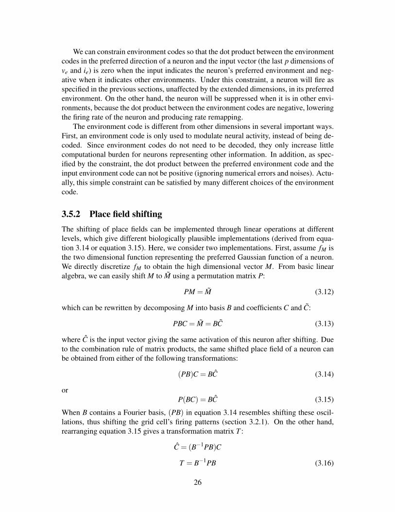
3.5.2 Place field shiftingThe shifting of place fields can be implemented through linear operations at differentlevels, which give different biologically plausible implementations (derived from equa-tion 3.14 or equation 3.15). Here, we consider two implementations. First, assume fM isthe two dimensional function representing the preferred Gaussian function of a neuron.We directly discretize fM to obtain the high dimensional vector M. From basic linearalgebra, we can easily shift M to M using a permutation matrix P:

PM = M (3.12)

which can be rewritten by decomposing M into basis B and coefficients C and C:

PBC = M = BC (3.13)

where C is the input vector giving the same activation of this neuron after shifting. Dueto the combination rule of matrix products, the same shifted place field of a neuron canbe obtained from either of the following transformations:

(PB)C = BC (3.14)

orP(BC) = BC (3.15)

When B contains a Fourier basis, (PB) in equation 3.14 resembles shifting these oscil-lations, thus shifting the grid cell’s firing patterns (section 3.2.1). On the other hand,rearranging equation 3.15 gives a transformation matrix T :

C = (B−1PB)C

T = B−1PB (3.16)

26

(a) (b)

(c)

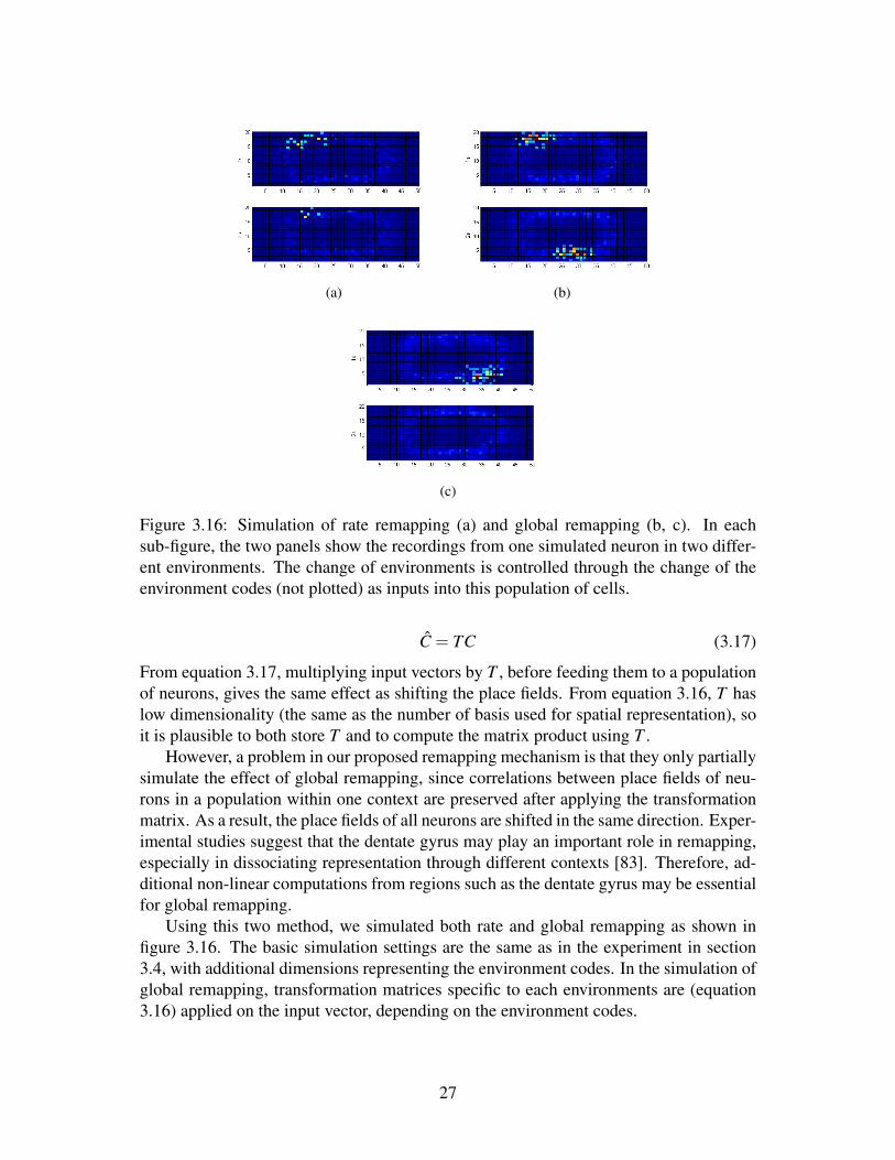
Figure 3.16: Simulation of rate remapping (a) and global remapping (b, c). In eachsub-figure, the two panels show the recordings from one simulated neuron in two differ-ent environments. The change of environments is controlled through the change of theenvironment codes (not plotted) as inputs into this population of cells.

C = TC (3.17)

From equation 3.17, multiplying input vectors by T , before feeding them to a populationof neurons, gives the same effect as shifting the place fields. From equation 3.16, T haslow dimensionality (the same as the number of basis used for spatial representation), soit is plausible to both store T and to compute the matrix product using T .

However, a problem in our proposed remapping mechanism is that they only partiallysimulate the effect of global remapping, since correlations between place fields of neu-rons in a population within one context are preserved after applying the transformationmatrix. As a result, the place fields of all neurons are shifted in the same direction. Exper-imental studies suggest that the dentate gyrus may play an important role in remapping,especially in dissociating representation through different contexts [83]. Therefore, ad-ditional non-linear computations from regions such as the dentate gyrus may be essentialfor global remapping.

Using this two method, we simulated both rate and global remapping as shown infigure 3.16. The basic simulation settings are the same as in the experiment in section3.4, with additional dimensions representing the environment codes. In the simulation ofglobal remapping, transformation matrices specific to each environments are (equation3.16) applied on the input vector, depending on the environment codes.

27

Chapter 4

Hippocampal replay

In this chapter, we explore the computational potential of the dense recurrent connectionsin the CA3 region of the hippocampus. Recurrent Neural Networks (RNN) initializedwith random weights are trained by the state-of-the-art Hessian Free optimization algo-rithm (HF) to simulate both forward and backward replay. While this chapter focuses onreplay itself, the relationship between replay and reinforcement learning is discussed insection 5.2.

4.1 The hippocampus as an information processing sys-tem

If we consider episodic memory as sequences of vectors (as described in the sectionsbefore), the anatomical structure (section 2.1) of the hippocampus gives some hints froman engineering view. When seen as an information processing system, this structureprovides an ideal setup for time series processing, such as continuously predicting: whilethe local recurrent connections at the CA3 provide control for the whole system, theglobal feedback loops are able to continually feed the output of the system back as theinput. In fact, researchers studying the hippocampus as a dynamic system have proposedthat the CA3 with recurrent connections implements an attractor [71, 24]. However, theseattractor models more often emphasize on the auto-completion of spatial patterns ratherthan temporal associations between patterns through time.

The simplified anatomical structure of the CA3 resembles a recurrent neural network(RNN, figure 4.1), governed by the following equations:

yt =Whi · xt +Whh ·ht−1 +bh (4.1)

ht = tanh(yt) (4.2)

zt =Woh ·ht +bo (4.3)

where x is the input, Whi is the weight matrix connecting the input to hidden layer, Whhis the weight matrix for the recurrent connections at the hidden layer, b’s are biases, and

28

Figure 4.1: A recurrent neural network. x represent input units, h represents hidden unitsand y represents output units. The states of the hidden units depend on both current inputand the last state of the hidden units.

z is the output. In theory, being hidden Markov models [69], RNNs are able to modelcomplex dynamics of temporal sequences. Elman [26] compares RNNs and other neuralnetwork models that are used to model temporal sequences. He concludes from both the-oretical reasoning and experimental simulations that RNNs can model complex temporaldynamics by representing the effect of time in their hidden layers, providing contextinformation discovered from the structure of temporal sequences. Therefore, given thatepisodic memory can be seen as temporal sequences, it is reasonable to explore how suchsequences can be stored and retrieved in RNNs, seeking insight into the computationalpotential of the recurrent connections in the hippocampus.

4.2 Training the RNNAlthough the potential of RNNs is promising from the above discussion, the trainingof RNNs is notoriously difficult. The most basic algorithm is back-propagation thoughtime (BPTT) [68, 74, 88, 89]. In general, BPTT unrolls a RNN, treating it as a multi-layer neural network with the same number of layers as the number of time steps in thetraining sequences, while keeping weight matrices connecting layers the same. Unfor-tunately, even worse than the unsatisfactory performance of back-propagation in deepnetworks [40] (see also appendix B), training RNNs for temporal sequences with longtemporal dependencies (more than 10 time steps) using BPTT is usually disappointing[8]. However, long temporal dependance is important given the length of a usual mem-ory episode. In the analysis by [42], they conclude that the difficulties in training RNNsusing gradient based methods mainly come from the “diminishing gradients” - the gradi-ents used as a training signal usually either explode or diminish when propagating. Sincestep sizes in gradient based (first-order) methods are proportional to the gradients, it isthus very difficult to choose suitable step sizes (appendix A). Because of this fundamen-tal problem, many previous algorithms for training RNNs are hardly better than randomguessing [41].

A breakthrough came from a method called long short-term memory (LSTM)[42],which introduces additional structures to regulate gradients (figure 4.2). Specifically,local unit recurrent connections are used to ensure that the gradientwill neither explode

29

nor diminish. With additional structural complexity, the LSTM is able to learn very longtemporal dependancies, and produces the state-of-the-art result in applications such asphoneme classification.

Another way to regularize gradients, without introducing any additional structure,is to use the second-order (curvature) information. The basic idea behind all second-order algorithms (e.g., Newton’s method, quasi-Newton methods, the conjugate gradientmethod [10] and the Hessian free optimization [56] used in this thesis), is to calculatestep sizes based on information from both first-order and second-order information. Ingeneral, when optimizing the parameters of a model in its parameter space, second-orderalgorithms take small steps when the curvature is large, where the gradient changes fast,and take large steps when the curvature is small, where the gradient changes slowly.Therefore, despite that gradients alone may still explode or diminish, the step sizes mod-ulated both by gradients and curvatures usually remain stable.

Due to the broad range of techniques used in the Hessian free optimization algorithm(HF), here we only treat HF as a black box, optimizing the neural network based ongiven training inputs and targets. A self-contained introduction of HF covering mostmathematical details is presented in appendix E.

4.3 Simulations of forward replayOur first goal is to simulate the forward replay (section 2.4). We use the followingphysical motion equation to generate random sequences in our experiments:

d2xdt2 =

FR

m(4.4)

where vector x is the position of a moving particle in a n dimensional space with massm at time t, and FR is a random force driving this particle. The random force FR allowsautomatically generating different random sequences, while the inertia from a non-zeromass m guarantees that some temporal correlation will be preserved. We can thereforeregard traces of these moving particles as memory episodes in a n dimensional memoryspace.

Since the global feedback loop (section 4.1) of the hippocampus is continually send-ing the output of the RNN to its input, we only need to train the RNN to predict one stepahead. For supervised learning of temporal sequences, this means, in the training set, thetarget sequence needs to be one step ahead of the input sequence. In the brain, such atraining set can be realized by introducing a delay at the input end. In addition, if theinput sequence is incomplete, such that it contains only some of the input dimensions,the learning can still proceed. In this case, the RNN learns to complete the pattern (i.e.pattern completion) at each time step, in addition to predicting future time steps (figure4.4).

We train RNNs with 150 hidden units, five input units and five output units witha batch containing all the sequences to be learned. Each of these sequences has 20time steps and five independent dimensions generated from equation 4.4. We define the

30

(a)

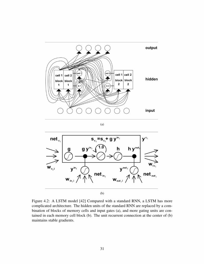
(b)

Figure 4.2: A LSTM model [42] Compared with a standard RNN, a LSTM has morecomplicated architecture. The hidden units of the standard RNN are replaced by a com-bination of blocks of memory cells and input gates (a), and more gating units are con-tained in each memory cell block (b). The unit recurrent connection at the center of (b)maintains stable gradients.

31

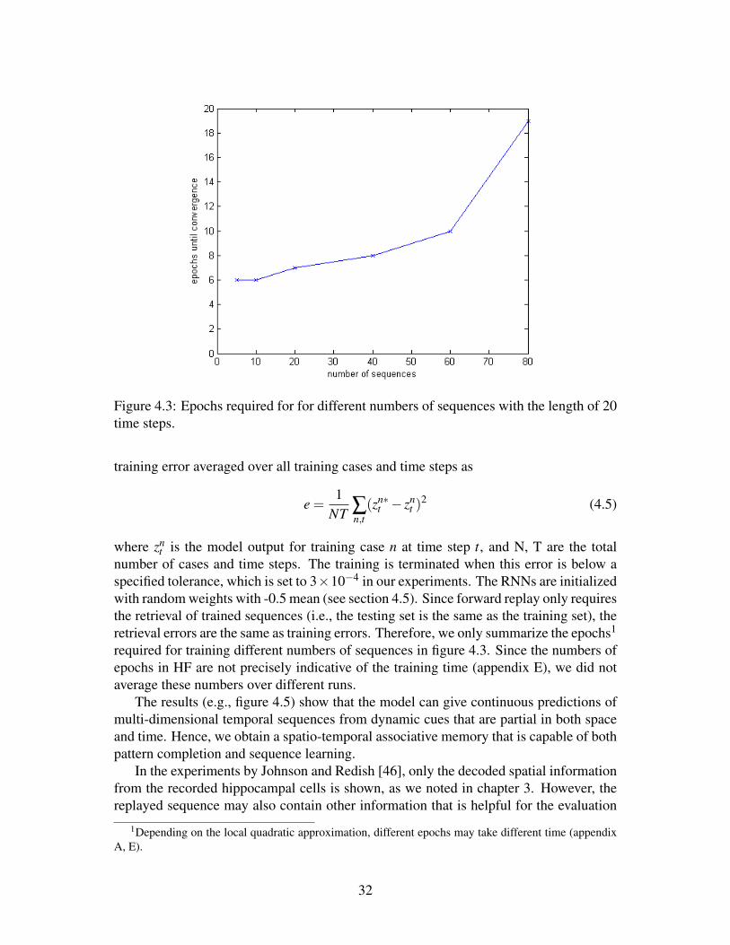
Figure 4.3: Epochs required for for different numbers of sequences with the length of 20time steps.

training error averaged over all training cases and time steps as

e =1

NT ∑n,t(zn∗

t − znt )

2 (4.5)

where znt is the model output for training case n at time step t, and N, T are the total

number of cases and time steps. The training is terminated when this error is below aspecified tolerance, which is set to 3×10−4 in our experiments. The RNNs are initializedwith random weights with -0.5 mean (see section 4.5). Since forward replay only requiresthe retrieval of trained sequences (i.e., the testing set is the same as the training set), theretrieval errors are the same as training errors. Therefore, we only summarize the epochs1

required for training different numbers of sequences in figure 4.3. Since the numbers ofepochs in HF are not precisely indicative of the training time (appendix E), we did notaverage these numbers over different runs.

The results (e.g., figure 4.5) show that the model can give continuous predictions ofmulti-dimensional temporal sequences from dynamic cues that are partial in both spaceand time. Hence, we obtain a spatio-temporal associative memory that is capable of bothpattern completion and sequence learning.

In the experiments by Johnson and Redish [46], only the decoded spatial informationfrom the recorded hippocampal cells is shown, as we noted in chapter 3. However, thereplayed sequence may also contain other information that is helpful for the evaluation

1Depending on the local quadratic approximation, different epochs may take different time (appendixA, E).

32

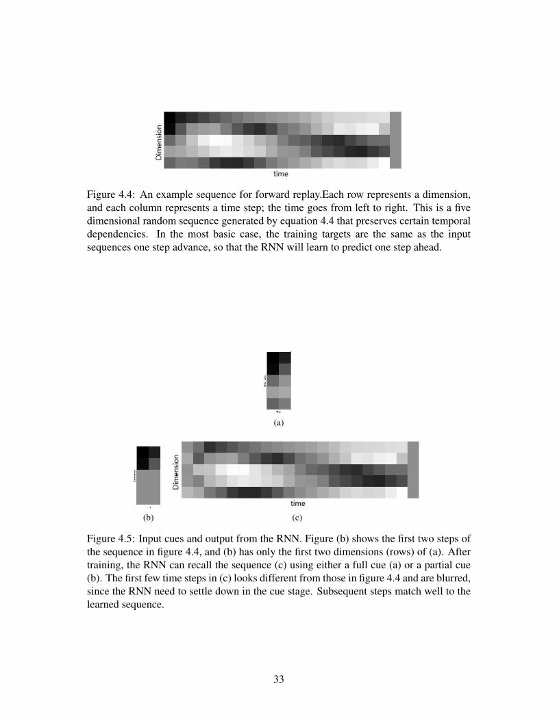
Figure 4.4: An example sequence for forward replay.Each row represents a dimension,and each column represents a time step; the time goes from left to right. This is a fivedimensional random sequence generated by equation 4.4 that preserves certain temporaldependencies. In the most basic case, the training targets are the same as the inputsequences one step advance, so that the RNN will learn to predict one step ahead.

(a)

(b) (c)

Figure 4.5: Input cues and output from the RNN. Figure (b) shows the first two steps ofthe sequence in figure 4.4, and (b) has only the first two dimensions (rows) of (a). Aftertraining, the RNN can recall the sequence (c) using either a full cue (a) or a partial cue(b). The first few time steps in (c) looks different from those in figure 4.4 and are blurred,since the RNN need to settle down in the cue stage. Subsequent steps match well to thelearned sequence.

33

of future reward [86]. We thus assign the third dimension of the replayed temporal se-quences (the third row in figure 4.6 (a)) a signal directly related to reward, so that themagnitude of this signal and the expected reward are directly correlated. Note this as-sumption is only used to illustrate how a rich representation in the memory can facilitatereward related computation. Figure 4.6 shows the simulation of the T-maze forward re-play. At the upper-right corner of 4.6 (h), the light red color indicates that the rewardsignal is strong enough so that the rat will make the decision to go right.

4.4 Simulations of reverse replayThe RNN can be trained in a similar way for both forward (section 2.4) and reversereplay2 (section 2.5), but problems arise when considering the functional role of reversereplay in reinforcement learning as well as experimental data. For example, since reversereplay was observed immediately after a rat reaches the goal after very limited training[21, 29], such a short time-scale is demanding for synaptic change-based recording ofexperiences. On the other hand, since the reversely replayed experience is usually shortand recent, it may be well stored through persistent neural activity rather than synapticweights. Therefore, the RNN for reverse replay is trained (or “pre-wired”, to distinguishit from the training for forward replay) differently, so that no more training is required inlater reverse replay.

For the reason discussed above, we wish the RNN to be able to replay any sequenceit recently experienced3. Since reverse replay often happens after a goal or a reward isreached, we assume it is triggered by an additional input signal. An example of an inputtraining sequence and its target is illustrated in figure 4.7. In order to ensure that the RNNis general enough to replay any input sequence (within a certain range), a training batchwith a large enough amount of sample sequences is necessary. Accordingly, although thetraining for reverse replay takes place only once, it is significantly more difficult than thetraining for forward replay.

In our experiments, we train RNNs with 150 hidden units, two input units and oneoutput units on 300 sequences similar to the one in figure 4.7. With other parameters thesame as in the RNNs for forward replay, we train the RNNs until convergence.

As examples, the two plots in figure 4.8 show reverse replay for two random se-quences with different length in the same RNN. Recall that this RNN is only trained forsequences with fewer than six time steps, so, interestingly, when sequences with greaterthan six time steps are presented, only the last few steps of the original sequences arereplayed correctly (figure 4.9). Given that only recent experience need to be reverselyreplayed, such dynamics are plausible.

In the reverse replay experiments in this thesis, we trained the RNN to replay onedimensional sequences with fewer than 6 time steps. Furthermore, our experiment illus-trates the extreme case in which the sequences are entirely random without any tempo-

2Since remote reverse replay (section 2.5) can be implemented in a way similar to the forward replay,by storing experiences in synapses, it is not discussed in this chapter.

3We trained different RNNs for forward and backward replay. Although they could be combined usinggating mechanisms [10], we leave that to future work as it is not directly related to our current focus.

34

(a) (b)

(c) (d)

(e) (f)

(g) (h)

Figure 4.6: Simulation of decision-point forward replay. In (a) and (b), the two 4-dimensional sequences (plotted in the same way as in figure 4.4) represent the replayalong the left and right arm respectively. In these two sequences, the first two dimensionsrepresent the locations (coordinates) of the rat, the third dimension represents the rewardrelated signal, where white means high reward. The fourth dimension are randomly gen-erated (equation 4.4) and used as context cues to recall the whole sequences. Figures (c)and (d) show the two cues used to recall the two sequences in (a) and (b). They are thefirst three steps of the fourth dimension in the input sequences. Figures (e)-(h) plot the4 time slices in process of replaying the sequences in (a) and (b) consecutively in a 2Dpanel. The location of each circle is specified by the first two dimensions, and the colorof these circles indicates the strength of the reward signal in the third dimension (redmeans high reward).

35

(a)

(b)

Figure 4.7: An example input sequence and its target for reverse replay. Figure (a) showsthe two dimensional input, in which the first dimension represents events to be replayedand the second dimension controls the commencing of the reverse replay through a mark(the while square). Figure (b) shows the target (desired output) used in training, speci-fying the reversed order of the events (compare the two red squares). Errors occurringin the time steps outside the red square are ignored as irrelevant noise. Note that the se-quence is completely random, exemplifying the extreme case of no temporal correlationat all.

ral correlation, although in the real world this is unlikely. In the brain, some synapticchanges may take place before reverse replay [21, 29], which could tailor the neural net-works for specific task structures. In summary, the training (or pre-wiring) for reversereplay in the brain could be significantly easier than in our experiment by taking advan-tage of more specific temporal structure. Nevertheless, our results show that the RNN ispowerful enough for a fairly general case.

To demonstrate the overall performance of reverse replay, we trained two RNNs withexactly the same procedures, testing them with random sequences at different lengths,and calculating the averaged mean square errors over 200 samples for each length. Whencalculating the errors we only consider at most the last 6 steps in the original experiences.Figure 4.10 shows the averaged errors for the 2 RNNs. For both RNNs the replay errorsare bounded around 0.1, which confirms the performance of long sequences shown infigure 4.9.

The fundamental difference between RNNs for forward and backward replay is thatexperiences are stored in synaptic weights for forward replay, but in neural activity alonefor reverse replay. On the one hand, forward replay needs longer time to learn because ofthe required synaptic change, but this brings the benefit that once learned, the sequencecan be recalled in a later time as long as the synaptic weights are not altered. On theother hand, reverse replay without synaptic change is fast, at the cost of being morevulnerable to interference – any alternation of the neural activity may affect the reversereplay. This trade-off between time and stability implies their different functional roles,which is worth further investigation.

Based on our simulation results, we predict that reverse replay does not require synap-tic change. This prediction is experimentally testable through injection of NMDA block-ers, which obstruct synaptic change, before testing trials or before training. In our pre-diction, the injections before testing trials will not affect reverse replay, but the injectionbefore initial training in a new environment may disrupt it.

36

(a) (b)

Figure 4.8: Simulation of reverse replay of 1D sequences, where the vertical axis repre-sents values at each time step. Figure (a) shows the reverse replay of a 4 step sequence,and (b) shows the reverse replay of a 6 step sequence from the same RNN. The symmetrybetween the blue lines (experience) and red lines (output) shows the replay is successfuleven in our extreme examples, although with observable distortions. Black dots outsideof the red line are irrelevant output noise (output before the start of reverse replay).

(a) (b)

Figure 4.9: Simulation of reverse replay for long sequences. Since the RNN is trained forsequences with length up to 6 time steps, only the last few steps of the original sequenceare replayed correctly, when a much longer sequence is used as input.

37

(a) (b)

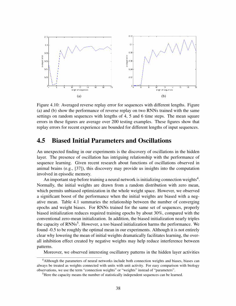
Figure 4.10: Averaged reverse replay error for sequences with different lengths. Figure(a) and (b) show the performance of reverse replay on two RNNs trained with the samesettings on random sequences with lengths of 4, 5 and 6 time steps. The mean squareerrors in these figures are average over 200 testing examples. These figures show thatreplay errors for recent experience are bounded for different lengths of input sequences.

4.5 Biased Initial Parameters and OscillationsAn unexpected finding in our experiments is the discovery of oscillations in the hiddenlayer. The presence of oscillation has intriguing relationship with the performance ofsequence learning. Given recent research about functions of oscillations observed inanimal brains (e.g., [37]), this discovery may provide us insights into the computationinvolved in episodic memory.

An important step before training a neural network is initializing connection weights4.Normally, the initial weights are drawn from a random distribution with zero mean,which permits unbiased optimization in the whole weight space. However, we observeda significant boost of the performance when the initial weights are biased with a neg-ative mean. Table 4.1 summaries the relationship between the number of convergingepochs and weight biases. For RNNs trained for the same set of sequences, properlybiased initialization reduces required training epochs by about 30%, compared with theconventional zero-mean initialization. In addition, the biased initialization nearly triplesthe capacity of RNNs5. However, a too biased initialization harms the performance. Wefound -0.5 to be roughly the optimal mean in our experiments. Although it is not entirelyclear why lowering the mean of initial weights dramatically facilitates learning, the over-all inhibition effect created by negative weights may help reduce interference betweenpatterns.

Moreover, we observed interesting oscillatory patterns in the hidden layer activities

4Although the parameters of neural networks include both connection weights and biases, biases canalways be treated as weights connected with units with unit activity. For easy comparison with biologyobservations, we use the term “connection weights” or “weights” instead of “parameters”.

5Here the capacity means the number of statistically independent sequences can be learned.

38

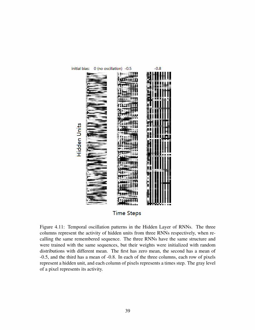
Figure 4.11: Temporal oscillation patterns in the Hidden Layer of RNNs. The threecolumns represent the activity of hidden units from three RNNs respectively, when re-calling the same remembered sequence. The three RNNs have the same structure andwere trained with the same sequences, but their weights were initialized with randomdistributions with different mean. The first has zero mean, the second has a mean of-0.5, and the third has a mean of -0.8. In each of the three columns, each row of pixelsrepresent a hidden unit, and each column of pixels represents a times step. The gray levelof a pixel represents its activity.

39

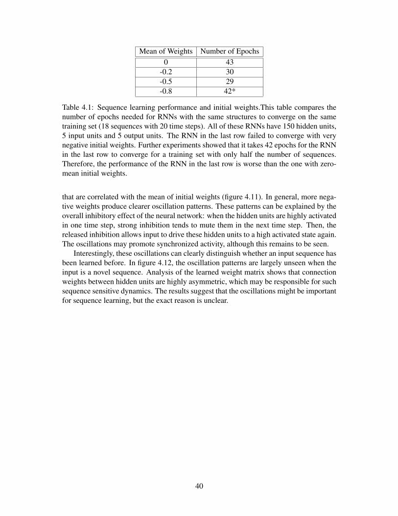
Mean of Weights Number of Epochs0 43

-0.2 30-0.5 29-0.8 42*

Table 4.1: Sequence learning performance and initial weights.This table compares thenumber of epochs needed for RNNs with the same structures to converge on the sametraining set (18 sequences with 20 time steps). All of these RNNs have 150 hidden units,5 input units and 5 output units. The RNN in the last row failed to converge with verynegative initial weights. Further experiments showed that it takes 42 epochs for the RNNin the last row to converge for a training set with only half the number of sequences.Therefore, the performance of the RNN in the last row is worse than the one with zero-mean initial weights.

that are correlated with the mean of initial weights (figure 4.11). In general, more nega-tive weights produce clearer oscillation patterns. These patterns can be explained by theoverall inhibitory effect of the neural network: when the hidden units are highly activatedin one time step, strong inhibition tends to mute them in the next time step. Then, thereleased inhibition allows input to drive these hidden units to a high activated state again.The oscillations may promote synchronized activity, although this remains to be seen.

Interestingly, these oscillations can clearly distinguish whether an input sequence hasbeen learned before. In figure 4.12, the oscillation patterns are largely unseen when theinput is a novel sequence. Analysis of the learned weight matrix shows that connectionweights between hidden units are highly asymmetric, which may be responsible for suchsequence sensitive dynamics. The results suggest that the oscillations might be importantfor sequence learning, but the exact reason is unclear.

40

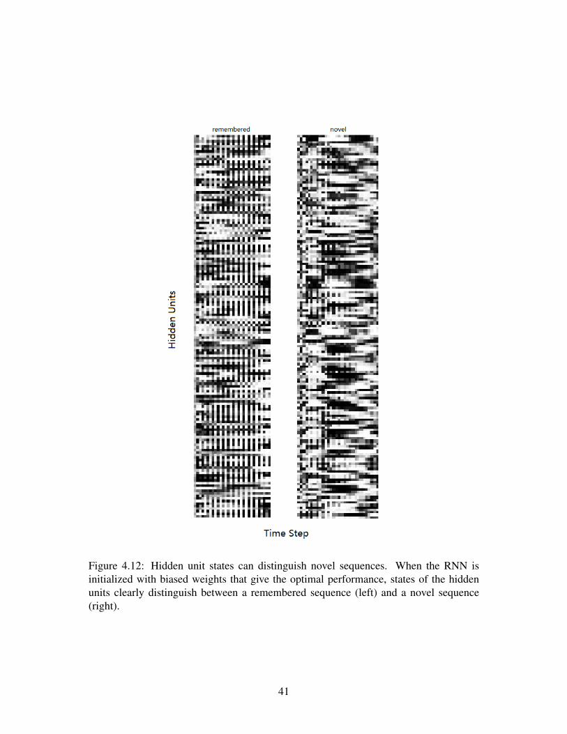
Figure 4.12: Hidden unit states can distinguish novel sequences. When the RNN isinitialized with biased weights that give the optimal performance, states of the hiddenunits clearly distinguish between a remembered sequence (left) and a novel sequence(right).

41

Chapter 5

Discussion

The interactions between hippocampus and other brain areas, especially the neocortex arenecessary in understanding brain functions such as various kinds of learning. However,limited by the scope of this thesis, our model mainly addresses the hippocampus itself.This chapter briefly outlines how our hippocampus model can be extended to shed lighton more general issues in neuroscience.

5.1 The hippocampus and the neocortexThe interaction between the hippocampus and the neocortex is crucial in coordinatingthe brain’s memory system. Classical computational models of memory systems [65, 59]suggest that the hippocampus and the neocortex play complementary roles [81].

In the framework proposed in [59], and further developed by [65], the hippocam-pus rapidly learns experienced input as episodes (episodic memory), which later slowlyconsolidates into the neocortex. In their proposal, an important purpose of the memorysystem is to learn the structural relations from patterns in experiences, forming knowl-edge that is able to benefit an animal in various ways. Although the neocortex is supposedto be mainly responsible for learning such structural relations, from both psychologicalexperiments and simulations using artificial neural networks, this learning process has tobe slow in order to both learn deep structural relations associating different patterns andnot to disrupt previously learned associations. This slow learning rate makes the neocor-tex incapable of learning directly from experiences without the help of a buffer systemthat rapidly stores experiences in the first place. The hippocampus provides such a tem-poral buffer for the neocortex, by quickly storing experiences without much processing(see also [55, 90]).

The different functional roles of the hippocampus and the neocortex propose distinctstructural requirements. In addition to a slow learning rate in the neocortex, a hierarchicalstructure is also helpful in discovering higher order relations (e.g. [40, 74]). On theother hand, as discussed before, the hippocampus has to be able to learn quickly, and adeep structure is not necessary. However, recurrent connections are necessary to formtemporal associations across a long time-span, as demonstrated in 4.

Moreover, the representations required by the hippocampus and the neocortex seem

42

to be fundamentally different. For the neocortex, distributed representations are bene-ficial because it is easier to discover associations between different patterns from over-lapped representation brought about by distributed representations [39]. However, sincethe main task of the hippocampus is to store near “raw” experiences as memory episodes,or a sequence of patterns, the main priority is to reduce the interference between differentepisodes. As a result, instead of being distributed, the neural representations in the hip-pocampus are sparse, i.e., only a very small portion of hippocampal neurons are activeat the same time, so that different patterns are more likely to be represented by differentneurons. In our model, we use vectors representing functions with a specific shape (e.g.,Gaussian function) to enforce the sparsity (chapter 3); in the hippocampus, the spar-sity constraint due to both similar representation schemes and the interactions betweendentate gyrus and CA3 that are not yet well known[61].

Both sparse firing patterns and remapping contribute to the broader mechanism ofpattern separation. While different patterns will be represented distinctly under the sparsefiring of hippocampal neurons, patterns that are similar but occur in different contexts,will also be represented differently because of remapping. As discussed earlier, the den-tate gyrus, a part of the hippocampal formation sending input to the CA3 region of thehippocampus, is one of the only two brain regions that are able to generate new neurons(neurogensis) in adult mammals [2]. Adult neurogenesis in the dentate gyrus may playan important role in pattern separation by further orthogonalizing the input from the en-torhinal cortex [1, 7, 83]. Together, the sparsity of firing and remapping provide the basisfor pattern separation that to a large extent guarantees experiences in the memory willnot interfere with each other [50].

Interestingly, pattern completion, a function that is also important for episodic mem-ory and demonstrated by experiments, functionally contradicts pattern separation [32,65, 73]. Through pattern completion, input that that only partly matches the originalexperiences may give rise to the same neural activities, i.e., the same episodic memory[63]. In this way, pattern completion allows more robust and flexible representations,as incomplete input patterns that are possibly caused by noise or changing environmentmay be recovered. Pattern completion can be implemented as attractors in computationalmodels [16, 24, 71]. Because pattern separation and pattern completion are competingdemands when an input pattern comes, a decision needs to be made concerning whetherthe pattern should be stored as a new pattern (pattern separation) or rather be used asa cue to access previously stored patterns (pattern completion). This decision may bereflected in different states of the hippocampus that are governed by a combination ofneural oscillations and other neurophysiology processes [61].

5.2 The hippocampus and reinforcement learningBoth forward and reverse replay may have a close connection with reinforcement learn-ing. As discussed in [86], in forward replay (section 2.4), the hippocampus may supporta forward model generating informative expectancies of the agent’s (e.g. a rat’s) futurestates. The co-activation of cells in ventral striatum signaling reward at the time of replay(or sweep) implies that the expectancies were evaluated by the ventral striatum, which

43

may implement the critic in the Actor-critic architecture. Given the rich informationthat can be encoded in the state space (as in the memory space, chapter 3), model-basedlearning based on this forward model should support flexible behaviors. The ability toincorporate both external and internal information in the state space permits learning ofdecision-making tasks modulated by latent variables such as internal motivation.

In contrast, since no synaptic change is required, reverse replay introduced in section4.4 enables fast association between reward and actions in recent past. The relativelyshort time-scale of reverse replay compared to forward replay may well support the com-putation needed by temporal difference learning [82]. Due to the difficulties involved intraining (or pre-wiring) a RNN for fast reverse replay (section 4.4), both the length andcomplexity of the replayed sequence is limited. Therefore, we suggest that, unlike for-ward replay that generates expectancies with rich information about the environment,reverse replay only associates significant actions and values. From this point of view,reverse replay may better support model-free reinforcement learning.

For the more general control problem, the hippocampus may be involved in all threekinds of controls: model-based, caching-based and episodic control [18, 48, 49]. How-ever, different control strategies may be implemented through different mechanisms inthe hippocampus (e.g., forward vs. reverse replay), so the transition between differ-ent control strategies becomes an additional issue [18]. In addition, especially for themodel-based control, a full forward model requires the coordination between differentbrain areas in addition to the hippocampus [19] (e.g., [44]), so a more comprehensivememory model incorporating semantic memory is likely required to better understandthe interaction between memory and reinforcement learning [59, 73, 47, 19].

5.3 Comparison with other modelsTo our knowledge, apart from our model, only [37] addressed both multi-modal repre-sentations and sequence learning. In this very recent model, Hasselmo unifies nearlyall experimental findings about the hippocampus, from the molecular to system level.Specifically, the central role of entorhinal cortex in his model gives insights into oscilla-tions in the hippocampus. Based on different model design choices, his biologically re-alistic model has physiologically grounded accounts of inputs from different modalities,rather than a unified representation scheme at a higher level as in our model. However,restricted by the biologically plausible Hebbian learning rules that is impossible to takeadvantage of second-order information, as well as the seemingly under-utilized CA3 re-current connections, his model is computationally less powerful than ours, which meansour model can encode more complex and longer memory episodes.

Another relatively comprehensive hippocampus model comes from Levy and col-leagues [51]. Levy’s model simulated high-level hippocampal functions including re-play from biologically plausible neural networks trained by elegant biologically plausiblelearning rules specifically derived for learning associative memory [52]. In addition tothe hippocampus itself, his model also addresses interactions between the hippocampusand the neocortex, proposing two forms of sequence compression mechanisms (on-lineand off-line compression). However, he uses ad-hoc style context and inhibitory neurons

44

that are neither biologically nor mathematically well justified. Similarly restricted by thebiologically plausible Hebbian learning rules, his model only demonstrates the replay ofrather simple sequences [5].

45

Chapter 6

Conclusions

Since the proposal of the hippocampus encoding a generic “memory” space [22], re-searchers have generally accepted that the hippocampus can encode information fromdifferent modalities. However, only a few computational model to date address this issue(e.g., [37]). Our model, using the Neural Engineering Framework (NEF), is the onlyone to our knowledge incorporating multi-modal information in a unified and systematicmanner. Our systematic approach makes the behavior of the model easy to characterizeby identifying specific mathematical operations. For example, neural integrators can beused to control temporal dynamics of the model representations [24], and transformationmatrices can be constructed to account for the shift of place fields.

Based on this systematical representation scheme, we further explored the dynamicssupporting storage and retrieval of sequences of vectors as episodic memory. Comparedto previous models based on gradient-descent-like Hebbian rules (e.g., [87, 5, 37]), webenefit from the state-of-the-art Hessian-Free Optimization algorithm (HF) [57, 58], re-sulting much more powerful temporal information processing. Therefore, it is currentlythe only hippocampus model able to replay long multi-dimensional sequences, support-ing the hypothesis proposed in [86] from a computational perspective, linking reactiva-tion of hippocampal activities to reinforcement learning problems. In addition, this isalso the first model demonstrating a RNN can replay recent temporal sequences usingpersistent neural activities only. Based on these results, we make a testable predictionthat the forward and reverse replay are supported by different mechanisms, in which onlyforward replay (and possibly “remote” reverse replay [17, 33]) requires synaptic change.

As the first adaptation of the HF algorithm in computational neuroscience, this thesisprovides an additional reference for challenging machine learning problems related toRNNs, and is of merit methodologically in neuroscience research. In order to betterintroduce the powerful HF method, the author derived most related techniques in theappendix part of this thesis, aiming to present this algorithm in a intuitive and relativelyeasy to understand way without losing necessary mathematical rigor. This self-containedtext on HF is another contribution of this thesis.

Due to time constraints, we have not fully integrated the representation and sequenceprocessing parts of the model. However, they are entirely compatible: they share thesame vector representations, and estimation of gradients can be applied to train neuralnetworks in NEF (Appendix B). In the future, we expect to continue exploring interac-

46

tions between parts of a wider memory system and the ways in which memory systemsare used in reinforcement learning.

47

Appendix

48

Appendix A

Quadratic functions

Quadratic functions provide good approximations to other higher-order functions, whileremaining simple enough to maintain the good properties we shall soon discuss. As aresult, they are used as a basic case in our following derivations of the back-propogationand the conjugate gradient method.

This appendix introduces some basic properties of quadratic functions that will behelpful in understanding general optimization methods. A quadratic function, f (x) :Rn→ R, has the following form:

f (x) = c+bx+12

x>Ax (A.1)

Despite its simple form, when equation A.1 is used as the second-order approximation(e.g., from Taylor’s expansion) of a higher-order function, the curvature information iswell preserved in matrix A. The quadratic function has gradients

g(x) = ∇ f (x) = b+Ax (A.2)

Equation A.2 holds true only when A is symmetric (otherwise ∇ f (x) = b+ 12(A+A>)x

). Here it is reasonable to assume the symmetry, because when used for approximation,matrix A (either a Hessian matrix or an approximation of Hessian such as a Gauss-Newton matrix) is always symmetric.

A symmetric matrix has the nice property of having a full set of orthonormal eigen-vectors:

Aui = λiui (A.3)

ui ·u j =

{0 i 6= j1 i = j

, for i, j = 1, 2, ...N (A.4)

where A is a n×n symmetric matrix, u are eigenvectors and λ are eigenvalues. Becauseof the orthogonality, the N eigenvectors span the whole N dimensional space.

Assuming that x∗is the point where the gradient ∇ f (x) of this quadratic function iszero, we expand equation A.1 at x∗:

f (x) = f (x∗)+12(x− x∗)>A(x− x∗) (A.5)

49

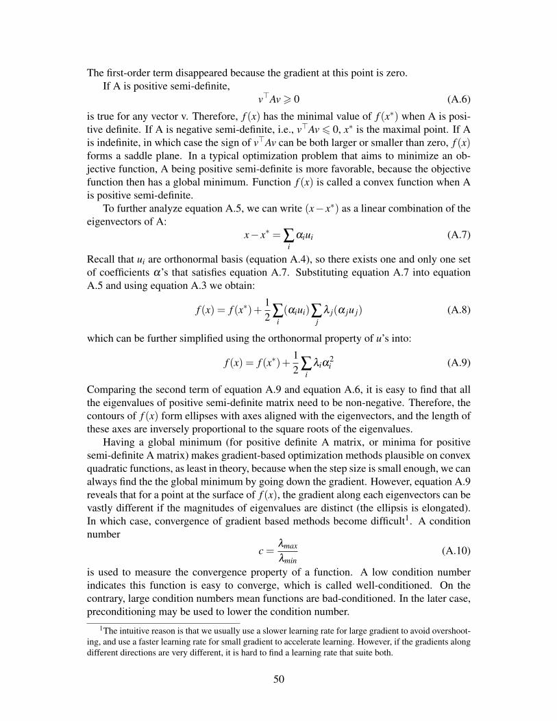
The first-order term disappeared because the gradient at this point is zero.If A is positive semi-definite,

v>Av > 0 (A.6)

is true for any vector v. Therefore, f (x) has the minimal value of f (x∗) when A is posi-tive definite. If A is negative semi-definite, i.e., v>Av 6 0, x∗ is the maximal point. If Ais indefinite, in which case the sign of v>Av can be both larger or smaller than zero, f (x)forms a saddle plane. In a typical optimization problem that aims to minimize an ob-jective function, A being positive semi-definite is more favorable, because the objectivefunction then has a global minimum. Function f (x) is called a convex function when Ais positive semi-definite.

To further analyze equation A.5, we can write (x− x∗) as a linear combination of theeigenvectors of A:

x− x∗ = ∑i

αiui (A.7)

Recall that ui are orthonormal basis (equation A.4), so there exists one and only one setof coefficients α’s that satisfies equation A.7. Substituting equation A.7 into equationA.5 and using equation A.3 we obtain:

f (x) = f (x∗)+12 ∑

i(αiui)∑

jλ j(α ju j) (A.8)

which can be further simplified using the orthonormal property of u’s into:

f (x) = f (x∗)+12 ∑

iλiα

2i (A.9)

Comparing the second term of equation A.9 and equation A.6, it is easy to find that allthe eigenvalues of positive semi-definite matrix need to be non-negative. Therefore, thecontours of f (x) form ellipses with axes aligned with the eigenvectors, and the length ofthese axes are inversely proportional to the square roots of the eigenvalues.

Having a global minimum (for positive definite A matrix, or minima for positivesemi-definite A matrix) makes gradient-based optimization methods plausible on convexquadratic functions, as least in theory, because when the step size is small enough, we canalways find the the global minimum by going down the gradient. However, equation A.9reveals that for a point at the surface of f (x), the gradient along each eigenvectors can bevastly different if the magnitudes of eigenvalues are distinct (the ellipsis is elongated).In which case, convergence of gradient based methods become difficult1. A conditionnumber

c =λmax

λmin(A.10)

is used to measure the convergence property of a function. A low condition numberindicates this function is easy to converge, which is called well-conditioned. On thecontrary, large condition numbers mean functions are bad-conditioned. In the later case,preconditioning may be used to lower the condition number.

1The intuitive reason is that we usually use a slower learning rate for large gradient to avoid overshoot-ing, and use a faster learning rate for small gradient to accelerate learning. However, if the gradients alongdifferent directions are very different, it is hard to find a learning rate that suite both.

50

Appendix B

Back-propagation in NEF

In this appendix, we present detailed derivation of the back-propagation algorithm inNEF. A two-layer toy neural network is used as an example to illustrate how parame-ters of NEF models can be learned through back-propagation of errors. Following thisexample, possible generalization of this derivation, including back-propagation throughtime (BPTT), is briefly discussed. To make this part self-contained, necessary equationsappearing in the main text are repeated. Since the neural networks in NEF can be re-garded as an extension of traditional artificial neural networks with additional notationsto characterize the heterogeneity and multi-dimensional responses, this derivation alsoapplies to simpler neural networks that are common in machine learning.

B.1 NotationsFigure B.1 shows the toy neural network for which we will derive learning rules for all itsparameters. This neural network maps an input vector X = (x1, x2, ..., xi, ...)

T , throughthe neural dynamics of two layers of LIF neurons, p1, p2, ..., p j, · · · and q1, q2, ..., qk, ...,to an output vector Y = (y1, y2, ..., yl, ...)

T .Given a constant input current, the firing ratea of a LIF neuron is determined by its

activation function G(J), as described inB.1. Parameters τre f , τRC, and Jthreshold are hold

Figure B.1: A toy neural network

51

Figure B.2: The activation function G(J) of a LIF neuron and it’s approximated first-order derivative G′(J)∗.

constant in the derivation 1.

a = G(J) =1

τre f − τRCln(1− JthresholdJ )

(B.1)

In order to use this activation function in the back-propagation algorithm, we needits first derivative. Although we can write the analytical form of G(J)’s first deriva-tive as in equation B.2, note that G(J) is not differentiable at the threshold point, wherelimJ→Jtrheshold+G′(J) = ∞. As a result, we need to approximate G′(J) by G′(J)∗that gen-erally preserved the shape of G′(J) (figure B.2), as shown in equation B.3(ξ and φ aresmall positive constants)

G′(J) =τRC · Jthreshold

(1− JthresholdJ ) · J2

/D2 (B.2)

D = τre f − τ

RCln(1− Jthreshold

J)

G′(J)∗ =

{G′(J) J > ξ

φ J < ξ(B.3)

For neurons receiving external input directly, such as neuron p j, the input current isgiven by the equation below, where e j is the encoder with the same length as the inputvector X , and b is the input bias of neuron p j. If we view the bias term as a neuron thatalways has unit activity, we can see the bias magnitude as the weight of connection to

1In most simulations, these parameters remain constants. We can learn them through calculating thegradients ofG(x) w.r.t. these parameters, but the process is not given in this appendix.

52

this unit activity neuron. Therefore, The bias term can be learned the same way as otherconnection weights. For this reason, we will not derive separated learning rule for biasterms.

We can simplify it by combine the gain factor g jand an element of e j to form gainfactors, αi j, for each element in the input vector, thus gives equation B.5. The encoderand the gain factor can be easily factored out after learning given the magnitude of eitherof them.

Jpj = γ j · eT

j ·X +bpj (B.4)

Jpj = ∑

iαi j · xi +bp

j (B.5)

For neurons receiving input from other neurons, their input currents are given byweighted sum of incoming activities. For example, the input current of neurons qk isdescribed by equation B.6, where w jk is the connection weights between neuron p jandqk.

Jqk = ∑

jw jk ·ap

j +bqk (B.6)

The output, Y , is decoded from linear combination of neural activities in the q layer.This decoding process is governed by decoders, dkl , as described in equation B.7

yl = ∑k

dkl ·aqk (B.7)

To sum up, parameters of this toy neural network are: gain factors αi j, connectionweights w jk, and decoders dkl .2 Given a set of desired outputs Y ∗ The goal of supervisedlearning in this toy neural network is to find proper parameters so that the model outputsY are as close to Y ∗as possible.

B.2 The Back-propagation AlgorithmNow we are going to derive the back-propagation algorithm for each parameter intro-duced in the last section. The algorithm can be divided into forward pass and backwardpass. In the forward pass, we run through the neural network by applying the equationsdescribed before, obtaining a model output Y . Then we can calculated the output errorby comparing it with the desired output Y ∗, and back-propagate this error to places thatneed error signal to facilitate training.

More formally, learning is achieved through optimizing, maximizing for minimizing,an objective function. The objective function, for minimizing, of the supervised learn-ing problem described above can be written as equation B.8. To make model outputsapproach desired outputs, the first term is the sum of the squared error for each outputelement across each training case c. Since large connection weights can make gradient

2As explained before, we treat bias terms as connection weights.

53

descent unstable, we also add the second term, the sum of all connection weights, topenalized large connection weights. In the following derivation, we will drop the sum-mation of cases to simplify the notations.

E =12 ∑

c∑

l(yc

l − yc∗l )2 +

12

λ ∑j∑k(w jk)

2 (B.8)

To determine how E is affected by each element of Y , we take the partial derivativewith respect to yl:

∂E∂yl

= yl− y∗l (B.9)

Given equation B.9 and equation B.7, we can calculate the partial derivative w. r. t.the decoder dkl using the chain rule:

∂E∂dkl

=∂E∂yl· ∂yl

∂dkl= (yl− y∗l ) ·a

qk (B.10)

The effect on E from the activation of aqkon yl is:

∂E∂yl· ∂yl

∂aqk= (yl− y∗l ) ·dkl (B.11)

Since aqk acts on all y’s, to take into account all the decoders interact with neuron qk:

∂E∂aq

k= ∑

l

∂E∂yl· ∂yl

∂aqk= ∑

l(yl− y∗l ) ·dkl (B.12)

Then we can then use the approximated gradient, equation B.3, to compute ∂E∂Jq

k:

∂E∂Jq

k=

∂E∂aq

k·

∂aqk

∂Jqk

(B.13)

= ∑l(yl− y∗l ) ·dkl ·G′(J)∗

Similarly, the following equations can derive by applying the chain rule and previousderived intermediate results:

∂E∂w jk

=∂E∂Jq

k·

∂Jqk

∂w jk+

∂12λ ∑ j ∑k(w jk)

2

∂w jk(B.14)

= ∑l(yl− y∗l ) ·dkl ·G′(J)∗ ·ap

j +λw jk

∂E∂ap

j= ∑

j

∂E∂Jq

j·

∂Jqj

∂apj

(B.15)

= ∑j∑k(yl− y∗l ) ·dkl ·G′(J)∗ ·w jk

54

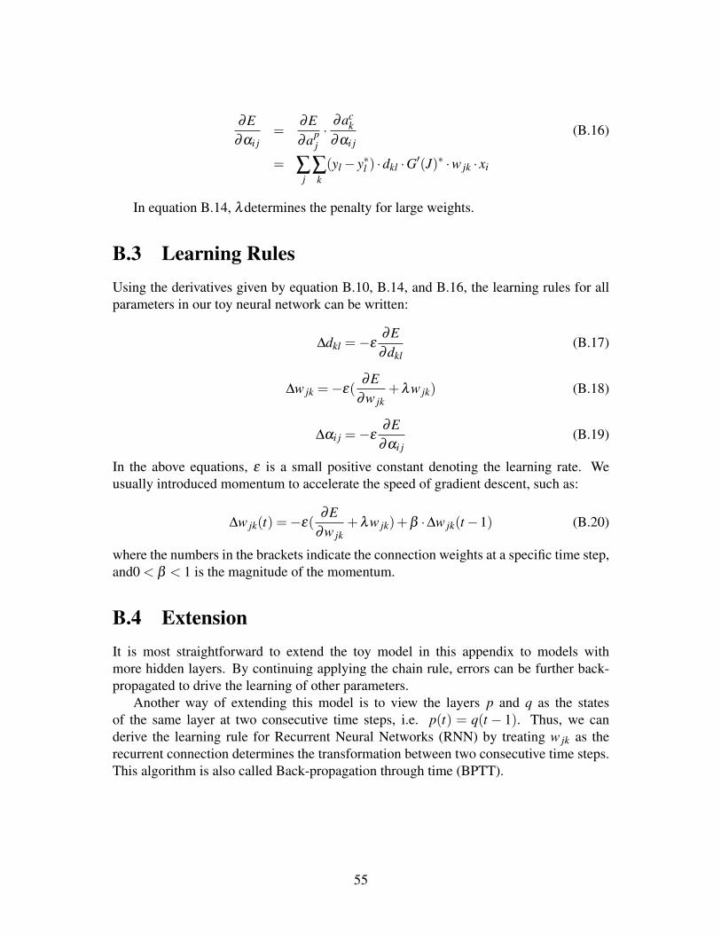
∂E∂αi j

=∂E∂ap

j·

∂ack

∂αi j(B.16)

= ∑j∑k(yl− y∗l ) ·dkl ·G′(J)∗ ·w jk · xi

In equation B.14, λdetermines the penalty for large weights.

B.3 Learning RulesUsing the derivatives given by equation B.10, B.14, and B.16, the learning rules for allparameters in our toy neural network can be written:

∆dkl =−ε∂E∂dkl

(B.17)

∆w jk =−ε(∂E

∂w jk+λw jk) (B.18)

∆αi j =−ε∂E

∂αi j(B.19)

In the above equations, ε is a small positive constant denoting the learning rate. Weusually introduced momentum to accelerate the speed of gradient descent, such as:

∆w jk(t) =−ε(∂E

∂w jk+λw jk)+β ·∆w jk(t−1) (B.20)

where the numbers in the brackets indicate the connection weights at a specific time step,and0 < β < 1 is the magnitude of the momentum.

B.4 ExtensionIt is most straightforward to extend the toy model in this appendix to models withmore hidden layers. By continuing applying the chain rule, errors can be further back-propagated to drive the learning of other parameters.

Another way of extending this model is to view the layers p and q as the statesof the same layer at two consecutive time steps, i.e. p(t) = q(t − 1). Thus, we canderive the learning rule for Recurrent Neural Networks (RNN) by treating w jk as therecurrent connection determines the transformation between two consecutive time steps.This algorithm is also called Back-propagation through time (BPTT).

55

Appendix C

Conjugate Gradients

The conjugate gradient method (CG) is the optimizer at the heart of the powerful Hessian-Free optimization algorithm. By utilizing second-order information, it is guaranteed toreach the global minimum of a quadratic error function in n steps, where n is the inputdimensionality of a function. For higher-order functions, such as the objective functionsof most neural networks, the non-linear version the conjugate gradient method is signifi-cantly more efficient than algorithms utilizing only first-order information (basic gradientdescent, such as Appendix B). Additionally, it is more economical in both computationand storage compared to quasi-Newton methods.

This self-contained appendix gives derivations of the conjugate gradient algorithmthat are essential for understanding the Hessian-Free optimization algorithm. It can alsobe used as a brief introduction to the conjugate gradient method. For a more comprehen-sive version, see the excellent introduction by [79].

C.1 Linear conjugate gradient methodsLet us start from the most basic linear CG, where the function to be minimized, f (x) :RN→R, has the following quadratic form of equation A.1, with the gradient of equationA.2. From basic calculus, a convex function f (x) reaches its minimum value f (x∗)(AppendixA) when its gradient

g(x∗) = b+Ax∗ = 0 (C.1)

However, the direct evaluation of x∗ = − bA

1is not plausible for large-scale problems,where the inversion of A is too expensive. As a result, we seek iterative methods to com-pute x∗numerically. In the following derivation, we write g(xi) as gi when appropriate.

The two central problems are

1. which direction we should search;

2. how large a step we should take along that direction.

1 This is a special case of Newton’s method.

56

C.1.1 Line searchFirst, we look at how to find an optimal step size αi, at step i, given a search directiondi. In other words, we try to find a value αithat minimizes f (xi +αidi). By taking thedirectional derivative,

∂ f (xi+1)

∂α= 0

∂ f (xi +αidi)

∂αi= 0

g>i+1di = 0 (C.2)

then substituting equation A.2 to calculate the gradient,

(b+Axi+1)>di = 0

(b+A(xi +αidi))>di = 0

we obtain:

αi =−(b+Axi)

>di

d>i Adi(C.3)

This process is called line-search. If we use the opposite direction of the gradient at eachstep as d, the same direction as in gradient descent

di =−gi (C.4)

equation C.3 and equation C.4 give the steepest descent algorithm, which uses the cur-vature information (matrix A) to regularize step sizes.

Note that gi+1 and di being orthogonal means that after taking this step, we not onlyminimize f (x) along the direction of di, but also reduce the length (strictly speaking,square of length) of the gradient at its largest extent. Therefore, any change along di willlengthen gi+1, because they are already orthogonal. This can be proved by taking thederivative

∂ [g>i+1gi+1]

∂αi= 0 (C.5)

Equation C.5 has the same solution of equation C.3.

C.1.2 Conjugate directionsIn order to find the direction we should take at each step, we need to analyze the opti-mization problem in greater depth. Note that the following statement are equal in thecontext of minimizing a quadratic function f (x):

1. Minimizing f (x).

2. Reaching a point where where the gradient of f (x) is zero.

3. Reaching the minimal point x∗.

57

The first statement is at the highest level, but it may not give us enough insight into theoptimization problem. For example, if we try to reduce the value of f (x) directly at eachiteration using gradient descent, the performance can be very bad for functions with lowcondition numbers. On the contrary, the third statement is at the lowest level. However,it is impractical since we don’t know x∗ in advance. Therefore, only statement 2 at themiddle is left to guide us in selecting the directions to take.

Given a direction di and a step size αi from equation C.3, we can obtain the gradientat xi+1, gi+1. Following the discussion in the last paragraph, our goal is to find the nextstep that continues reducing the gradient length towards zero, with the constraint that thegradient already reduced by di (from gi) in the last step is not undone. From equationC.2, we infer this can be satisfied by keeping the gradient at the next step, gi+2, stillorthogonal to direction di, so that step i also minimizes gi+2, in addition to gi+1, alongits direction di.

g>i+2di = 0

g(xi+1 +αi+1di+1)>di = 0

[b+A(xi+1 +αi+1di+1)]>di = 0

(b+Axi+1)>di +αi+1d>i+1Adi = 0 (C.6)

From equation C.2, the first term of equation C.6 is zero. To guarantee the second termis also zero, directions di+1 and di must satisfy

d>i+1Adi = 0 (C.7)

Directions satisfying equation C.7 are said to be conjugate, and this is where the name“conjugate gradient” comes from.

To extend the previous argument using induction, since all the following steps alsoshould not undo the “work” by step i( along its direction di) we further require that

g>k di = 0 (C.8)

holds true for all k > 1. Applying equation C.6 repeatedly, we see all the search directionsmust satisfy the conjugacy condition

d>i Ad j = 0 f or i 6= j (C.9)

C.1.2.1 Search directions are linearly independent

We then prove that if A is positive definite, these search directions are linearly indepen-dent. Assuming these directions are not all linearly independent (reductio ad absurdum),there exists such dk that

dk =n

∑i=0

γidi (C.10)

where γi are constant coefficients and γk = 0. From equation C.9

d>k Ad j = 0 (C.11)

58

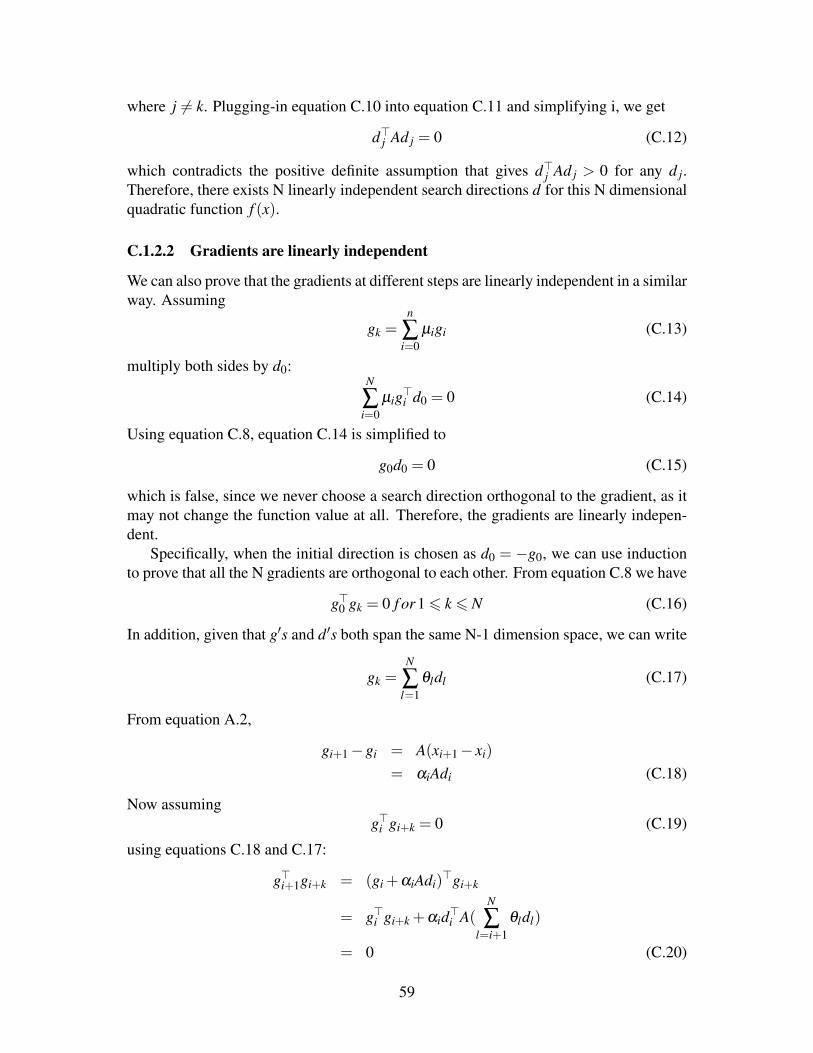
where j 6= k. Plugging-in equation C.10 into equation C.11 and simplifying i, we get

d>j Ad j = 0 (C.12)

which contradicts the positive definite assumption that gives d>j Ad j > 0 for any d j.Therefore, there exists N linearly independent search directions d for this N dimensionalquadratic function f (x).

C.1.2.2 Gradients are linearly independent

We can also prove that the gradients at different steps are linearly independent in a similarway. Assuming

gk =n

∑i=0

µigi (C.13)

multiply both sides by d0:N

∑i=0

µig>i d0 = 0 (C.14)

Using equation C.8, equation C.14 is simplified to

g0d0 = 0 (C.15)

which is false, since we never choose a search direction orthogonal to the gradient, as itmay not change the function value at all. Therefore, the gradients are linearly indepen-dent.

Specifically, when the initial direction is chosen as d0 = −g0, we can use inductionto prove that all the N gradients are orthogonal to each other. From equation C.8 we have

g>0 gk = 0 f or 1 6 k 6 N (C.16)

In addition, given that g′s and d′s both span the same N-1 dimension space, we can write

gk =N

∑l=1

θldl (C.17)

From equation A.2,

gi+1−gi = A(xi+1− xi)

= αiAdi (C.18)

Now assumingg>i gi+k = 0 (C.19)

using equations C.18 and C.17:

g>i+1gi+k = (gi +αiAdi)>gi+k

= g>i gi+k +αid>i A(N

∑l=i+1

θldl)

= 0 (C.20)

59

Together with equation C.16, g′s are orthogonal to each other.

g>i g j = 0 f or all i 6= j (C.21)

Note that many other derivations regard the orthogonality between gradients as an im-portant property of conjugate gradients, but actually this is only true when the initialdirection is the opposite of its gradient (d0 = −g0). Nevertheless, as proved in sectionC.1.4, the initial search direction generally does not affect the convergence of the conju-gate gradient method.

C.1.3 Constructing conjugate directionsAlthough in theory we can select the start direction d0 and the starting point x0 arbitrarily,the common practice is to start from x0 = 0 and initialize do =−g0. x0 = 0 guarantees thenon-constant part of the quadratic equation will be non-positive (actually 0) , providing agood starting point for minimization2. Taking the initial direction as the gradient ensuresthat the value of f (x) will reduce quickly and gives the nice property that all gradients areorthogonal, as shown in section C.1.2.2. In addition, since the gradient will be evaluatedin all the following steps (equation C.3), such initialization makes the whole processconsistent.

After d0 = −g0 is obtained, the following directions can be constructed one by oneusing the Gram-Schmidt process

di+1 = ui+1−i

∑k=0

βi+1,kdk (C.22)

where u′s are linearly independent vectors. Equation C.22 means we can construct aseries of conjugate directions3 by subtracting from a vector ui+1 the components of idirections previously obtained. Given the independence of gradients (section C.1.2.2),we use the gradients obtained at step i+ 1(gi+1) as ui+1 in equation C.22. Multiplyingboth sides of equation C.22 by d>i A, we can simplify it using conjugacy and orthogonality(equation C.8,C.9; here we drop the subscription k of β for simplicity)

0 = d>i Agi+1−βi+1d>i Adi

βi+1 =g>i+1Adi

d>i Adi(C.23)

Note that because of conjugacy between directions, β1, β2, ...βi are not relevant for con-structing consecutive conjugate directions. Therefore, equation C.22 can be written as

di+1 = ui+1−βi+1,kdk (C.24)

2However, for Hessian-Free optimization, there are even better initial points (section E.3).3Recall that the Gram-Schmidt process was first introduced to construct a set of orthogonal vectors.

Conjugacy sometimes are also called A-orthogonality, where A is the matrix at the middle of equationC.9. Actually, the basic idea underlying the Gram-Schmidt process allow it to construct vectors with anysuch orthogonal relationships.

60

The matrix-vector product in equation C.23 can be avoided using equation C.18

βi+1 =g>i+1(gi+1−gi)

d>i (gi+1−gi)(C.25)

which is known as the Hestenes-Stiefel expression. It can be simplified using equationC.8, C.24 to obtain the Polak-Ribiere form:

βi+1 =g>i+1(gi+1−gi)

g>j gi(C.26)

When we start with the opposite of the gradient as the initial direction, thus different gra-dients are orthogonal (equation C.21), the Polak-Ribiere form can be further simplifiedto the Fletcher-Reeves form

βi+1 =g>i+1gi+1

g>i gi(C.27)

All three expressions computing the coefficients β are the same when conjugacy betweendirection is strictly held. This condition is generally true in the linear case, where onlyminor numerical errors may affect conjugacy. Therefore, we usually use the simplestone, equation C.27, in linear conjugate gradients.

C.1.4 Convergence of conjugate gradientsThe conjugate gradient method is efficient because it is guaranteed to converge in n stepsfor n dimensional quadratic functions. Now we prove why this is true (equation C.3,C.23).

Suppose we have n conjugate directions d1, d2, ...dn constructed using equation C.23.Since they are linearly independent (section C.1.2.1), they span the n dimensional spacewhere function f (x) is defined. Therefore, we can find a set of steps αidi leading to thesolution x∗ from an initial point x0

x∗− x0 =n

∑i=1

αidi (C.28)

Multiply both sides by d>0 A and use equation C.1 to get rid of x∗

−d>0 (b+Ax0) =n

∑i=1

αid>0 Adi (C.29)

Again, using equation C.9, we simplify the above equation and solve for

α0 =−(b+Ax0)

>d0

d>0 Ad0(C.30)

Similarly, we can solve all the coefficients

αi =−(b+Axi)

>di

d>i Adi(C.31)

which is the same as equation C.3. Therefore, we proved the conjugate gradient methodconverges to the minimal point x∗ in N steps for any N dimensional quadratic function.

61

C.1.5 The conjugate gradient algorithmSince the derivation of conjugate gradients is quite complicated, here we summarize it inthe algorithm form. It may look slightly different from the derivation above because ofsome pre-multiplication in order to improve the performance.

1. Initialize the starting position x← x0

2. g← b+Ax

3. d←−g

4. δi← g>g

5. p← Ad

6. α ← δid>p

7. x← x+αd

8. g← g+α p

9. δi−1← δi

10. δi← g>g

11. β ← δiδi−1

12. d← r−βd

13. goto step 5 until meet stop condition

The stop condition in the last step can be reaching a certain precision or the maximumiterations. Another good choice of the termination condition is the on described in [57],which terminates the CG when the decrease of the objective function is small. It termi-nates CG at iteration i when the following inequities satisfy:

i > kφ(xi)< 0φ(xi)−φ(xi−k)

φ(xi)< kε

Where k = max(10, 0.1× i) and ε = 1e− 4 is chosen in the experiments in this thesis.The ε is smaller than that in [57], because the regression here requires higher precision.Although increasing ε may accelerate learning, a too large ε could produce low qualitysteps that slow down the learning and even make the Hessian-Free optimization fail toconverge.

62

C.2 Non-linear Conjugate gradient methodsMost practical problems, such as optimization in machine learning, are non-linear. Wecan apply the linear conjugate gradient method described before with only slight modifi-cation to the line-search and constructing conjugate direction steps.

For line-search, since the error surface is not quadratic, the first step one may temptto do is to substitute matrix A with the second-order derivative f ”(x), or the Hessianmatrix, the same as in the second-order expansion of f (x+δ ) at x

q(δ ) = f (x)+∇ f (x)>δ +δ>Hδ (C.32)

where δ is the increment at a step. In other words, if x represents parameters at thelast step, δ represents the increment of these parameters from the last step. However,equation C.3 is no longer able to minimize the error in one step. A simple solution isto apply equation C.3 repeatedly until the the change of error function after one step issmaller than a threshold value. This is actually the Newton-Raphson method. When thesecond-order derivative of f (x) is not available or too expensive to compute, one mayapproximate it using secant method or other line-search algorithms that do not dependon second order information (see [79] for more information).

As discussed in section C.1.3, all three expressions of the coefficients β (equationC.25, C.26 and C.27) are the same when conjugacy between directions is strictly held,which is generally true in linear cases. However, the conjugacy deteriorates fast in thenon-linear case, in which matrix A, thus the definition of conjugacy, is constantly chang-ing. In non-linear case, the Polak-Ribiere (equation C.26) form is found to performslightly better than the Fletcher-Reeves form. One reason might be that the assumptionof orthogonality between gradients, in order to obtain equation C.27, is usually not true,as discussed in section C.1.2.2.

When applying the modified steps above, since conjugacy between search directionsis no longer preserve, CG generally cannot converge in N steps. For this reason, a com-mon practice is to restart the conjugate gradient method after N steps. Despite the breakof conjugacy in non-linear problems, CG still has relatively good performance.

However, the non-linear conjugate gradient method, as well as many other second-order algorithms, has the problem that it may be trapped in local minima or even localmaxima. These unfavored behaviors can be explained using the conclusion from ap-pendix A: if the instantaneous Hessian at a step is negative-definite, the line-search willmove towards local maxima, increasing the error; if the Hessian is indefinite, the line-search may either increase or reduce the error. As a result, once the Hessian is notpositive-definite, which usually happens for highly non-linear functions, the behavior ofconjugate gradients (and many other second-order optimization algorithms) may not beas good as one may expect. Furthermore, even if the Hessian is always positive-definite,when the line-search is exact, the error function will go to local minima. On the otherhand, if the line-search is inexact, the conjugacy will deteriorate even faster.

63

Appendix D

An efficient way of computingmatrix-vector products

In the conjugate gradient method introduced in appendix C, many steps require com-puting the product between a matrix and a vector (e.g., step 2 and 5 in the algorithm inC.1.5). Since the matrix A in has the size of n×n for any n dimensional function f (x),simply accessing matrix A has the complexity O(n2). In large-scale problems, such astraining neural networks with a reasonable size, the size of A will be too large for bothstoring A and computing the matrix-vector product directly. This appendix introducesthe ℜ{·} operator[67] that efficiently computes matrix-vector products with linear com-plexity (O(n)).

We start our derivation with the first-order expansion of f (x+∆x) at x

f (x+∆x) = f (x)+ f ′(x)>∆x+O(||∆x||2) (D.1)

Because of the error term O(||∆x||2), the expansion above is exact. The expansion canbe rewritten by substituting ∆x with the product of a scalar r and a vector v

f (x+ rv) = f (x)+ f ′(x)>rv+O(||rv||2) (D.2)

Rearranging equation D.2 and dividing both sides by the scalar r, we obtain the productbetween f ′(x), a matrix, and the vector v1:

f ′(x)>v =f (x+ rv)− f (x)

r+O(|r|)

= limr→0

f (x+ rv)− f (x)r

(D.3)

where we further drop the error term and obtain the exact product by taking the limitr→ 0. Equation D.3 is actually the definition of the directional derivative of f (x) alongthe direction v. Therefore, we can define the ℜ{·} operator2

ℜv{ f (x)} ≡ ∂

∂ rf (x+ rv) |r=0 (D.4)

1In actual application in optimization, the matrix in the place of f ′(x) is usually a symmetric matrix,such as a Hessian or Gauss-Newton matrix.

2The subscript v in equation D.4 is usually omitted for simplicity when no confusion will occur.

64

Since ℜ{·} is a differential operator, rules of differential operators, such as chain rule,product rule, quotient rule also apply to it:

ℜ{c · f (x)}= cℜ{ f (x)}

ℜ{ f (x)+g(x)}= ℜ{ f (x)}+ℜ{g(x)}

ℜ{ f (x)g(x)}= ℜ{ f (x)}g(x)+ f (x)ℜ(g(x))

R{ f (g(x))}= f ′((g(x))ℜ{g(x)}

ℜ{d f (x)dt}= dℜ{ f (x)}

dtSpecifically,

ℜ{x}= v

can be proved by the definition in equation D.3, D.4

ℜ{x} = limr→0

(x+ rv)− xr

= v

It is exact the product(x)′v = Iv = v

A straightforward application of theℜ{·} is to compute the product between Hessianand another vector as a part of the nonlinear conjugate gradient method.

65

Appendix E

Hessian-Free Optimization

E.1 OverviewWith the background knowledge introduced in Appendices A, C and D, we can derive theHessian-Free optimization algorithm (HF). As discussed in section C.2, directly applyingthe non-linear conjugate gradient method or other second-order algorithms may result inunfavored behaviors caused by the Hessian matrices that are not positive semi-definite.To solve this problem, the general idea behind the Hessian-Free Optimization is to reg-ulate the local curvature (second-order) information, providing an ideal environment forthe conjugate gradient method1.

Following the discussion above, we functionally divide the Hessian-Free optimiza-tion into two steps: local quadratic approximation and optimization. In the first step, apositive-definite quadratic function is used to approximate the original non-linear objec-tive function locally. In the second step, we optimize the quadratic function obtainedin the first step using the linear conjugate gradient method. Since only the quadraticfunction is used for optimization, the convergence properties of the linear CG are wellpreserved.

E.2 Positive semi-definite approximationRecall that the problem of many second-order methods lies with the Hessian – it maynot be positive semi-definite. To solve this problem, we need to find a matrix guaranteedto be positive semi-definite as an approximation of the Hessian, and use this matrix inplace of the Hessian to approximate the original objective function. We start to find thispositive semi-definite matrix by analyzing the Hessian2.

1The conjugate gradient method, instead of other second order optimizer, is used here, because it isefficient in both storage and computation (both are linear) for large scale problems. A detailed comparisonof second-order methods is beyond the scope of this appendix. Please refer to text such as Chapter 7 of[10] for more detailed account of different optimization algorithms.

2In this appendix, we write the objective function as f (θ) instead of f (x) to more clear indicate ourpurpose of optimizing for parameters of a neural network.

66

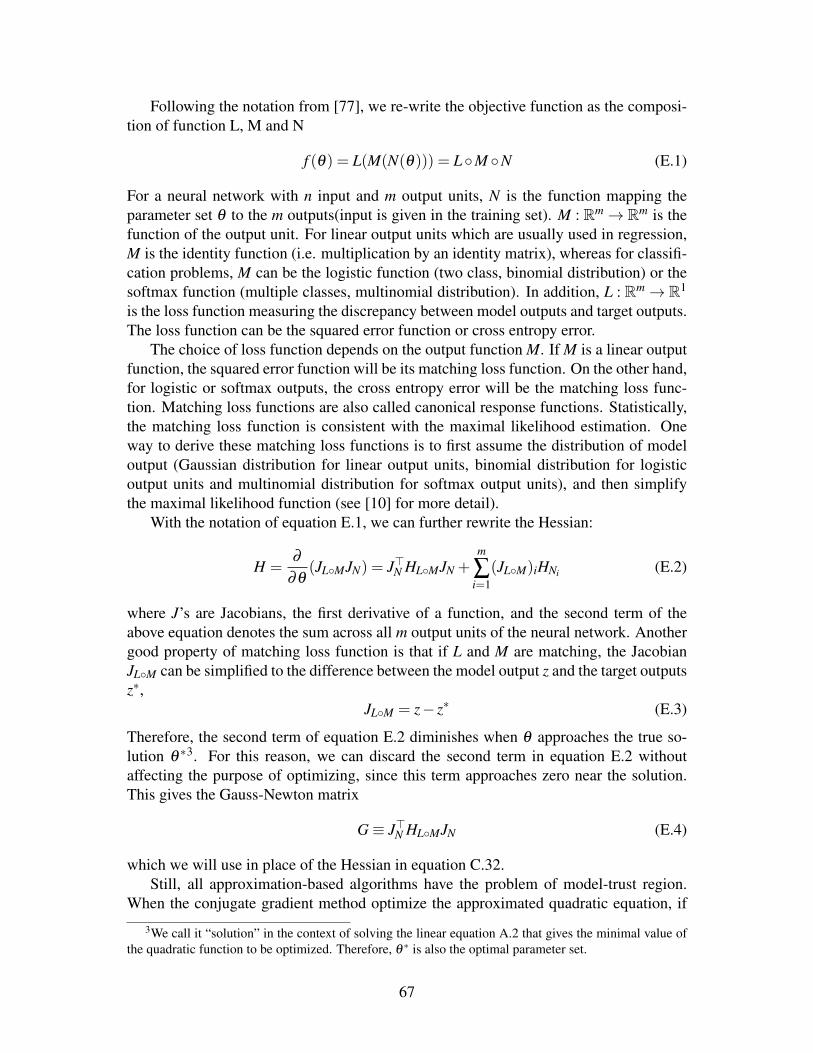
Following the notation from [77], we re-write the objective function as the composi-tion of function L, M and N

f (θ) = L(M(N(θ))) = L◦M ◦N (E.1)

For a neural network with n input and m output units, N is the function mapping theparameter set θ to the m outputs(input is given in the training set). M : Rm→ Rm is thefunction of the output unit. For linear output units which are usually used in regression,M is the identity function (i.e. multiplication by an identity matrix), whereas for classifi-cation problems, M can be the logistic function (two class, binomial distribution) or thesoftmax function (multiple classes, multinomial distribution). In addition, L : Rm→ R1

is the loss function measuring the discrepancy between model outputs and target outputs.The loss function can be the squared error function or cross entropy error.

The choice of loss function depends on the output function M. If M is a linear outputfunction, the squared error function will be its matching loss function. On the other hand,for logistic or softmax outputs, the cross entropy error will be the matching loss func-tion. Matching loss functions are also called canonical response functions. Statistically,the matching loss function is consistent with the maximal likelihood estimation. Oneway to derive these matching loss functions is to first assume the distribution of modeloutput (Gaussian distribution for linear output units, binomial distribution for logisticoutput units and multinomial distribution for softmax output units), and then simplifythe maximal likelihood function (see [10] for more detail).

With the notation of equation E.1, we can further rewrite the Hessian:

H =∂

∂θ(JL◦MJN) = J>N HL◦MJN +

m

∑i=1

(JL◦M)iHNi (E.2)

where J’s are Jacobians, the first derivative of a function, and the second term of theabove equation denotes the sum across all m output units of the neural network. Anothergood property of matching loss function is that if L and M are matching, the JacobianJL◦M can be simplified to the difference between the model output z and the target outputsz∗,

JL◦M = z− z∗ (E.3)

Therefore, the second term of equation E.2 diminishes when θ approaches the true so-lution θ ∗3. For this reason, we can discard the second term in equation E.2 withoutaffecting the purpose of optimizing, since this term approaches zero near the solution.This gives the Gauss-Newton matrix

G≡ J>N HL◦MJN (E.4)

which we will use in place of the Hessian in equation C.32.Still, all approximation-based algorithms have the problem of model-trust region.

When the conjugate gradient method optimize the approximated quadratic equation, if

3We call it “solution” in the context of solving the linear equation A.2 that gives the minimal value ofthe quadratic function to be optimized. Therefore, θ ∗ is also the optimal parameter set.

67

the step taken is too large (large δ in equation C.32), the approximation may be bad. Asa result, decrease in the (approximated) quadratic function may not be accompanied bya similar decrease in the objective function. We thus need to regularize the step size,usually by adding a Tikhonov term λδ>δ that penalizes large δ 4. After using the Gauss-Newton matrix, and adding the Tikhonov term, we obtain the objective function

q(δ ) = f (θ)+∇ f (θ)>δ +δ>(G+λ I)δ (E.5)

where I is the identity matrix.Worth noting that equation E.5 is the same as the objective function in the Levenberg-

Marquardt algorithm when the neural network has linear output units, where G = J>N JN .Therefore, we can understand the objective function in the Hessian-Free algorithm as anextension of the Levenberg-Marquardt algorithm to non-linear outputs5. The parameterλ in equation E.5 is also adjusted the same way as in the Levenberg-Marquardt algo-rithm: {

λ = cλ φ < 14

λ = 1c λ φ > 3

4(E.6)

where c is a positive value (c is usually set to 10 in the classical Levenberg-Marquardtalgorithm, and set to 4 in Hessian-Free), and the positive number

φ =the decrease of the quadratic functionthe decrease of the original function

The intuition behind this heuristic of adjusting theλvalue is that if the decrease in theobjective function is small compared to the decrease in the quadratic function, the ap-proximation is bad, so we need to increase λ to impose a more conservative step. Onthe contrary, if φ is already large enough, thus the approximation is accurate, larger stepscan accelerate the optimization.

In [58], another method called the structural damping is used in conjunction with theTikhonov term to further regularize the objective function for recurrent neural networks(RNN) by specifically penalizing the distortion compared with the non-linearity in thehidden layer of a RNN. However, We do not find it useful in the tasks in this thesis.Given that the structural damping is not a general approach, it is not presented here.

E.3 Optimization on quadratic approximationNow we can put everything together, optimizing an objective function f (θn) throughoptimizing its quadratic approximation qn(δ ) at each step using the conjugate gradientmethods. We stop the conjugate gradients once the value of qn(δ ) decreased to belowa tolerance value, thus obtaining a step δn. Next, we update both the approximatedquadratic function and parameters and optimize the new quadratic function qn+1 fromδn, where qn+1 is the approximation of the objective at θn+1 = θn + δn. Note that the

4It is also called L2 regularization, which is always written as 12 λ ||δ ||2

5However, the Levenberg-Marquardt algorithm does not use conjugate gradients as its optimizer.

68

optimization on qn+1 starts from the direction of the last step δn, instead of 0 (sectionC.1.3), since this initial direction usually significantly accelerates the conjugate gradientmethod in the Hessian-Free optimization [57]. The reason might be that qn+1 and qn aresimilar, so they are likely to have resembling minimal points.

In some situations, especially when the step-size becomes very small, the Tikhonovregularization is not enough to deal with the very high local non-linearity. In these cases,we shorten δn

6 through an inexact backtracking line-search to obtain a δ ∗n that betteraccommodates the local surface. The Wolfe conditions can be used to govern this inexactline search by finding a step length αk, so that δ ∗n =αkδn gives a sufficiently smaller valueof the objective function than δn. A step length αk is said to satisfy the Wolfe conditionsif

1.f (θn +αkδn)6 f (θn)+ c1αkδ

>n ∇ f (θn) (E.7)

2.δ>n ∇ f (θn +αkδn)> c2δ

>n ∇ f (θn) (E.8)

After the initialization α1 = 1, if any of the Wolfe conditions is violated, we update thestep length by backtracking αn+1 = ταn, where τ is a value smaller than 1 (0.7 in theexperiments in this thesis). Since the Wolfe condition is hard to satisfy, we usually limitthe times of backtracking performed (a limit of kmax = 5 is used here so that δ ∗n can notbe smaller than τ5δn).

E.4 Modified PassesBackpropagation is a way of applying chain rule to calculate derivatives of a function.In neural networks, the original backpropagation computes the gradient of an objectivefunction[74] (see also appendix B). Using the R-operator introduced in appendix D, wecan modify the original backward and forward passes to produce useful measures suchas Hessian, Fisher Information matrix or Gauss-Newton matrix[77].

As an example, this section gives detailed derivations of using forward and backpasses to calculate the product of a Gauss-Newton matrix and a vector v in a recurrentneural network with linear output units and squared error objective function. We assumethe hidden units using the tanh function. Equations for other structures (not necessarilyneural networks) can be derived in similar ways.

In the following equations, “·” denotes matrix multiplication, and “∗” denotes ele-ment wise multiplication.

6An additional “CG back-tracking” process is introduced in [57], in which the parameter is updated byδ ′n that is obtained from go back a few steps of the conjugate gradient methods until if the back-trackingprocess yields a smaller value of the original objective function. However, I found this process slowsdown the overall convergence, and some time even make a few problems failed to converge, so the CGback-tracking is not presented. The drawback of CG back-tracking might be a result of going back to localminima that ignored by the smoothy quadratic approximation.

69

E.4.1 Standard forward passThis is the standard forward pass a typical recurrent neural network.

Initialize h0 = 0, run from time step 1 to the last step T:

yt =Whi · xt +Whh ·ht−1 +bh (E.9)

ht = tanh(yt) (E.10)

zt =Woh ·ht +bo (E.11)

f = ∑t(zt− z∗t )

> · (zt− z∗t ) (E.12)

E.4.2 Standard backward passThe backward pass is obtained from take the derivative of the objective function usingthe chain rule. Note it uses intermediate results from the standard forward pass.

Initialize ∂ f∂yt+1

= 0, run from time step T backward to step 1:

∂ f∂ zt

= zt− z∗t (E.13)

∂ f∂ht

=Whh ·∂ f

∂yt+1+Woh ·

∂ f∂ zt

(E.14)

∂ f∂yt

= (1+hi)∗ (1−hi)∗∂ f∂ht

(E.15)

Only this line is responsible for structural damping:

∂ f∂yt

=∂ f∂yt

+λ µ(1+ht)∗ (1−ht)∗ yt (E.16)

∂ f∂Woh

=∂ f∂ zt·h>i (E.17)

∂ f∂bo

=∂ f∂ zt

(E.18)

∂ f∂Whh

=∂ f

∂yt+1·h>i (E.19)

∂ f∂bh

=∂ f∂yt

(E.20)

∂ f∂Whi

=∂ f∂yi· x>i (E.21)

70

E.4.3 R-forward passThe R-forward is derived from applying the R operator around equations for the standardforward pass. It uses intermediate results from both standard forward and backwardpasses.

InitializeR(h0) = 0

R(yt) = vWhi · xt + vWhh ·ht−1 +Whh ·R(ht−1)+ vbh (E.22)

R(ht) = (1+ht)∗ (1−ht)∗R(yt) (E.23)

R(zt) = vWoh ·ht +Woh ·R(hy)+ vbo (E.24)

E.4.4 R-backward passTo construct the product between the Gauss-Newton matrix and vector v, we only R-backpropagating through the loss function L , and then backpropagate in the standardway. The only step different from standard backward pass is that we initialize R( ∂ f

∂ zt) =

R(zt), rather than E.13. In calculating the Gauss-Newton matrix, this step can be under-stood as back-propagating the product JNv, as defined by ℜ{Zt} (equation D.4), insteadof the error as in the standard backward pass. It uses the intermediate results from allabove passes.

E.4.5 Mini-batchesAs described in section C.1.5, both the gradient and the matrix-vector product are calcu-lated for conjugate gradients. However, the matrix-vector products need to be evaluatedmuch more often than the gradients, since for each HF step (optimization on a givenquadratic equation) the gradient only need to be evaluated once while as the matrix-vector products need to be evaluated at each CG line-search step. Moreover, it’s clearfrom the above passes that the evaluation of matrix-vector product is more expensive thanevaluating the gradients. Therefore, it is reasonable too consider using smaller batches,as subsets of the full training batch, in evaluating the matrix-vector products, when thetraining batch is large.

E.5 The algorithmTo summarize this appendix, the steps in the Hessian-Free optimization are outlined here:

1. Randomly initialize parameters of a modelθ ; initialize the first step δ = 0.

2. Run CG on the quadratic function q approximated at f (θ), noting (see sectionC.1.5 for processes of CG):

71

(a) Start CG from q(δ )

(b) Evaluate the gradient g using standard backpropagation.

(c) Evaluate the matrix-vector product (such as G · v) used in CG by modifiedpasses.

(d) Terminate CG when stop condition of CG meets, obtaining a step δ .

3. Use inexact backtracking line-search guided by the Wolfe conditions to obtain δ ∗.

4. Update the parameters by θ = θ +δ ∗.

5. Go to step 2 until termination conditions of HF meets.

The termination conditions of HF, which terminate the whole learning process, is some-what task dependent. It usually includes reaching maximum epochs or exceeding a tol-erance of error.

72

References

[1] James B. Aimone, Janet Wiles, and Fred H. Gage. Computational influence of adultneurogenesis on memory encoding. Neuron, 61(2):187–202, January 2009. 3, 7,43

[2] Joseph Altman. Are new neurons formed in the brains of adult mammals? Science,135(3509):1127–1128, March 1962. 43

[3] Pablo Alvarez and Larry R. Squire. Memory consolidation and the medial temporallobe: a simple network model. Proceedings of the National Academy of Sciencesof the United States of America, 91(15):7041–5, July 1994. 3

[4] Per Anderson, Richard Morris, David Amaral, Tim Bliss, and John O’Keefe. Thehippocampus book. OXford University Press, 2007. 3, 4

[5] David A. August and William B. Levy. Temporal sequence compression by anintegrate-and-fire model of hippocampal area CA3. Journal of computational neu-roscience, 6(1):71–90, January 1999. 45, 46

[6] Arnold Bakker, C. Brock Kirwan, Michael Miller, and Craig E. L. Stark. Patternseparation in the human hippocampal CA3 and dentate gyrus. Science (New York,N.Y.), 319(5870):1640–2, March 2008. 3

[7] Suzanna Becker. A computational principle for hippocampal learning and neuro-genesis. Hippocampus, 15(6):722–38, January 2005. 7, 43

[8] Yoshua Bengio, Patrice Simard, and Paolo Frasconi. Learning long-term depen-dencies with gradient descent is difficult. IEEE transactions on neural networks / apublication of the IEEE Neural Networks Council, 5(2):157–66, January 1994. 29

[9] Chris M. Bird and Neil Burgess. The hippocampus and memory: insights fromspatial processing. Nature reviews. Neuroscience, 9(3):182–94, March 2008. 3, 7

[10] Christopher M. Bishop. Neural Networks for Pattern Recognition. OXford Univer-sity Press, 1996. 30, 34, 66, 67

[11] Neil Burgess, Caswell Barry, and John O’Keefe. An oscillatory interference modelof grid cell firing. Hippocampus, 17(9):801–812, 2007. 18

73

[12] Neil Burgess, Suzanna Becker, John A. King, and John O’Keefe. Memory forevents and their spatial context: models and experiments. Philosophical transac-tions of the Royal Society of London, 356(1413):1493–503, September 2001. 3,6

[13] Margaret F. Carr, Shantanu P. Jadhav, and Loren M. Frank. Hippocampal replayin the awake state: a potential substrate for memory consolidation and retrieval.Nature neuroscience, 14(2):147–53, February 2011. 2

[14] Neal J. Cohen and Howard Eichenbaum. Memory, Amnesia, and the HippocampalSystem. The MIT Press, 1993. 1, 3, 6

[15] Laura Lee Colgin, Edvard I. Moser, and May-Britt Moser. Understanding memorythrough hippocampal remapping. Trends in neurosciences, 31(9):469–77, Septem-ber 2008. 7, 8

[16] John Conklin and Chris Eliasmith. A controlled attractor network model of pathintegration in the rat. Journal of computational neuroscience, 18(2):183–203, 2005.17, 18, 43

[17] Thomas J. Davidson, Fabian Kloosterman, and Matthew A. Wilson. Hippocampalreplay of extended experience. Neuron, 63(4):497–507, 2009. 2, 9, 46

[18] Nathaniel D. Daw, Yael Niv, and Peter Dayan. Uncertainty-based competition be-tween prefrontal and dorsolateral striatal systems for behavioral control. Natureneuroscience, 8(12):1704–11, December 2005. 44

[19] Peter Dayan. Goal-directed control and its antipodes. Neural networks : the officialjournal of the International Neural Network Society, 22(3):213–9, April 2009. 44

[20] Sachin S. Deshmukh and Upinder S. Bhalla. Representation of odor habituationand timing in the hippocampus. The Journal of neuroscience : the official journalof the Society for Neuroscience, 23(5):1903–15, March 2003. 1

[21] Kamran Diba and György Buzsáki. Forward and reverse hippocampal place-cellsequences during ripples. Nature neuroscience, 10(10):1241–2, October 2007. 34,36

[22] Howard Eichenbaum, Paul Dudchenko, Emma Wood, Matthew Shapiro, andHeikki Tanila. The hippocampus, memory, and place cells: is it spatial memoryor a memory space? Neuron, 23(2):209–26, June 1999. 1, 6, 12, 46

[23] Arne D. Ekstrom, Micheal J. Kahana, Jeremy B. Caplan, Tony A. Fields, Eve A.Isham, Ehren L. Newman, and Itzhak Fried. Cellular networks underlying humanspatial navigation. Nature, 425(September), 2003. 1

[24] Chris Eliasmith. A unified approach to building and controlling spiking attractornetworks. Neural computation, 17(6):1276–314, June 2005. 23, 28, 43, 46

74

[25] Chris Eliasmith and Charles H. Anderson. Neural Engineering. The MIT Press,2004. 12, 15

[26] Jeffrey Elman. Finding Structure in Time. Cognitive Science, 211:179–211, 1990.20, 29

[27] André A. Fenton, Hsin-Yi Kao, Samuel a Neymotin, Andrey Olypher, YevgeniyVayntrub, William W Lytton, and Nandor Ludvig. Unmasking the CA1 ensem-ble place code by exposures to small and large environments: more place cellsand multiple, irregularly arranged, and expanded place fields in the larger space.The Journal of neuroscience : the official journal of the Society for Neuroscience,28(44):11250–62, October 2008. 4

[28] Ila R. Fiete, Yoram Burak, and Ted Brookings. What grid cells convey about ratlocation. The Journal of neuroscience : the official journal of the Society for Neu-roscience, 28(27):6858–71, July 2008. 20

[29] David J. Foster and Matthew A. Wilson. Reverse replay of behavioural sequences inhippocampal place cells during the awake state. Nature, 440(7084):680–3, March2006. 2, 9, 11, 34, 36

[30] Marianne Fyhn, Sturla Molden, Menno P. Witter, Edvard I. Moser, and May-BrittMoser. Spatial representation in the entorhinal cortex. Science (New York, N.Y.),305(5688):1258–64, August 2004. 20

[31] Lisa M. Giocomo, Eric A. Zilli, Erik Fransén, and Michael E. Hasselmo. Temporalfrequency of subthreshold oscillations scales with entorhinal grid cell field spacing.Science (New York, N.Y.), 315(5819):1719–22, March 2007. 18, 20

[32] April E. Gold and Raymond P. Kesner. The role of the CA3 subregion of the dorsalhippocampus in spatial pattern completion in the rat. Hippocampus, 15(6):808–14,January 2005. 43

[33] Anoopum S. Gupta, Matthijs A. A. van der Meer, David S. Touretzky, and A. DavidRedish. Hippocampal replay is not a simple function of experience. Neuron,65(5):695–705, March 2010. 6, 9, 46

[34] Torkel Hafting, Marianne Fyhn, Sturla Molden, May-Britt Moser, and Edvard I.Moser. Microstructure of a spatial map in the entorhinal cortex. Nature,436(7052):801–6, August 2005. 20

[35] Demis Hassabis, Carlton Chu, Geraint Rees, Nikolaus Weiskopf, Peter D.Molyneux, and Eleanor A. Maguire. Decoding neuronal ensembles in the humanhippocampus. Current biology : CB, 19(7):546–54, April 2009. 6

[36] Demis Hassabis, Dharshan Kumaran, Seralynne D. Vann, and Eleanor A. Maguire.Patients with hippocampal amnesia cannot imagine new experiences. Proceedingsof the National Academy of Sciences of the United States of America, 104(5):1726–31, January 2007. 6

75

[37] Michael E. Hasselmo. How we remember. MIT Press, 2011. 3, 38, 44, 46

[38] Micheal E. Hasselmo, Lisa M. Giocomo, and Eric A. Zilli. Grid cell firing mayarise from interference of theta frequency membrane potential oscillations in singleneurons. Hippocampus, 17(12):1252–1271, 2007. 20

[39] Geoffrey E. Hinton. Learning distributed representations of concepts. In R. G. M.Morris, editor, Parallel distributed processing: Implications for psychology andneurobiology, pages 46–61. Clarendon Press, Oxford, England, 1989. 43

[40] Geoffrey E. Hinton, Simon Osindero, and Yee-Whye Teh. A fast learning algorithmfor deep belief nets. Neural computation, 18(7):1527–1554, 2006. 29, 42

[41] Sepp Hochreiter and Paolo Frasconi. Gradient Flow in Recurrent Nets : the Di cultyof Learning Long-Term Dependencies 1 Introduction 2 Exponential error decayGradients of the error function. In John F. Kolen and Stefan C. Kremer, editors, AField Guide to Dynamical Recurrent Networks. Wiley-IEEE Press, 2001. 29

[42] Sepp Hochreiter and Jurgen Schmidhuber. Long short-term memory. Neural com-putation, 9(8):1735–80, November 1997. 29, 31

[43] Etsuro Hori, Yoichi Nishio, Kenichi Kazui, Katsumi Umeno, Eiichi Tabuchi, KazuoSasaki, Shunro Endo, Taketoshi Ono, and Hisao Nishijo. Place-related neural re-sponses in the monkey hippocampal formation in a virtual space. Hippocampus,15(8):991–6, January 2005. 2

[44] Daoyun Ji and Matthew A. Wilson. Coordinated memory replay in the visual cortexand hippocampus during sleep. Nature Neuroscience, 10(1):100–107, 2006. 44

[45] Adam Johnson and a David Redish. Hippocampal replay contributes to withinsession learning in a temporal difference reinforcement learning model. Neu-ral networks : the official journal of the International Neural Network Society,18(9):1163–71, November 2005. 2

[46] Adam Johnson and A. David Redish. Neural ensembles in CA3 transiently en-code paths forward of the animal at a decision point. The Journal of neuroscience,27(45):12176–89, November 2007. 8, 32

[47] Szabolcs Káli and Peter Dayan. Off-line replay maintains declarative memories in amodel of hippocampal-neocortical interactions. Nature neuroscience, 7(3):286–94,March 2004. 44

[48] Mate Lengyel and Peter Dayan. Hippocampal contributions to control: The thirdway. Advances in neural information processing systems, 20:889–896, 2007. 44

[49] Mate Lengyel and Peter Dayan. Performance analysis of alternative controllersTree-structured MDPs. In Advances in neural information processing systems,pages 1–22, 2009. 44

76

[50] Jill K Leutgeb, Stefan Leutgeb, May-Britt Moser, and Edvard I. Moser. Pattern sep-aration in the dentate gyrus and CA3 of the hippocampus. Science, 315(5814):961–6, February 2007. 43

[51] William B. Levy, Ashlie B. Hocking, and Xiangbao Wu. Interpreting hippocampalfunction as recoding and forecasting. Neural networks : the official journal of theInternational Neural Network Society, 18(9):1242–64, November 2005. 44

[52] William B. Levy and Oswald Steward. Synapses as associative memory elementsin the hippocampal formation. Brain research, 175:233–245, 1979. 44

[53] Christopher J. MacDonald, Kyle Q. Lepage, Uri T. Eden, and Howard Eichenbaum.Hippocampal "Time Cells" Bridge the Gap in Memory for Discontiguous Events.Neuron, 71(4):737–749, August 2011. 1, 4, 6, 7

[54] Ludise Malkova and Mortimer Mishkin. One-trial memory for object-place associ-ations after separate lesions of hippocampus and posterior parahippocampal regionin the monkey. The Journal of neuroscience : the official journal of the Society forNeuroscience, 23(5):1956–65, March 2003. 1, 6

[55] David Marr. From the Retina to the Neocortex. Citeseer, 1991. 42

[56] James Martens. A New Algorithm for Rapid Parameter Learning in Linear Dynam-ical Systems. PhD thesis, 2009. 30

[57] James Martens. Deep learning via Hessian-free optimization. In Proceedings ofthe 27th International Conference on Machine Learning (ICML), volume 951, page2010, 2010. 46, 62, 69

[58] James Martens and Ilya Sutskever. Learning Recurrent Neural Networks withHessian-Free Optimization. In Proceedings of the 28th International Conferenceon Machine Learning, 2011. 46, 68

[59] James L. McClelland, Bruce L. McNaughton, and Randall C. O’Reilly. Why thereare complementary learning systems in the hippocampus and neocortex: insightsfrom the successes and failures of connectionist models of learning and memory.Psychological review, 102(3):419–57, July 1995. 42, 44

[60] Matthew D. McEchron, Wilbur Tseng, and John F. Disterhoft. Neurotoxic lesionsof the dorsal hippocampus disrupt auditory-cued trace heart rate (fear) conditioningin rabbits. Hippocampus, 10(6):739–51, January 2000. 1

[61] Edvard I. Moser, Emilio Kropff, and May-Britt Moser. Place cells, grid cells, andthe brain’s spatial representation system. Annual review of neuroscience, 31:69–89,January 2008. 43

[62] John O’Keefe and Jonathan Dostrovsky. The hippocampus as a spatial map: Prelim-inary evidence from unit activity in the freely-moving rat. Brain Research, 34:171–175, 1971. 1, 4

77

[63] John O’Keefe and Lynn Nadel. The Hippocampus as a Cognitive Map. OXfordUniversity Press, 1978. 4, 43

[64] John O’Keefe and Lynn Nadel. Précis of O’Keefe & Nadel’s The hippocampus asa cognitive map. Behavioral and Brain Sciences, 2:487–494, May 1979. 1

[65] Randall C. O’Reilly and Jerry W. Rudy. Computational principles of learning inthe neocortex and hippocampus. Hippocampus, 10(4):389–97, January 2000. 42,43

[66] Eva Pastalkova, Vladimir Itskov, Asohan Amarasingham, and György Buzsáki. In-ternally generated cell assembly sequences in the rat hippocampus. Science (NewYork, N.Y.), 321(5894):1322–7, September 2008. 1, 4, 20

[67] Barak A. Pearlmutter. Fast exact multiplication by the Hessian. Neural Computa-tion, 6(1):147–160, 1994. 64

[68] Fernando J. Pineda. Generalization of back-propagation to recurrent neural net-works. Physical Review Letters, 59(19):2229–2232, 1987. 29

[69] L. R. Rabiner and B. H. Juang. An introduction to hidden Markov models. ASSPMagazine, IEEE, 3(1):4–6, June 1986. 29

[70] A. David Redish. Beyond the Cognitive Map. A Bradford Book, 1999. 1

[71] A. David Redish and David S. Touretzky. Cognitive maps beyond the hippocampus.Hippocampus, 7(1):15–35, January 1997. 28, 43

[72] Sébastien Royer, Anton Sirota, Jagdish Patel, and György Buzsáki. Distinct repre-sentations and theta dynamics in dorsal and ventral hippocampus. The Journal ofneuroscience, 30(5):1777–87, February 2010. 23

[73] Jerry W. Rudy and Randall C. O’Reilly. Contextual fear conditioning, conjunc-tive representations, pattern completion, and the hippocampus. Behavioral Neuro-science, 113(5):867, 1999. 43, 44

[74] David E. Rumelhart, Geoffrey E. Hinton, and Ronald J. Williams. Learning repre-sentations by back-propagating errors. Nature, 323(6088):533–536, 1986. 29, 42,69

[75] Alexei Samsonovich and Bruce L. McNaughton. Path integration and cognitivemapping in a continuous attractor neural network model. The Journal of neu-roscience : the official journal of the Society for Neuroscience, 17(15):5900–20,August 1997. 5

[76] Daniel L Schacter and Donna Rose Addis. The cognitive neuroscience of con-structive memory: remembering the past and imagining the future. Philosoph-ical transactions of the Royal Society of London. Series B, Biological sciences,362(1481):773–86, May 2007. 6

78

[77] Nicol N Schraudolph. Fast curvature matrix-vector products for second-order gra-dient descent. Neural computation, 14(7):1723–38, July 2002. 67, 69

[78] William Beecher Scoville and Brenda Milner. Lss of recent memory after bilateralhippocampal lesions. J. Neurol. Neurosurg. Psychiat., 20(11), 1957. 1

[79] Jonathan Richard Shewchuk. An Introduction to the Conjugate Gradient MethodWithout the Agonizing Pain. Technical report, 1994. 56, 63

[80] Trygve Solstad, Edvard I. Moser, and Gaute T. Einevoll. From Grid Cells to PlaceCells : A Mathematical Model. Hippocampus, 1031:1026–1031, 2006. 18, 20

[81] Larry R. Squire. Memory systems of the brain: a brief history and current per-spective. Neurobiology of learning and memory, 82(3):171–7, November 2004. 1,42

[82] Richard S. Sutton and Andrew Barto. Reinforcement Learning. MIT Press, 1998.44

[83] Alessandro Treves, Ayumu Tashiro, Menno P. Witter, and Edvard I. Moser. What isthe mammalian dentate gyrus good for? Neuroscience, 154(4):1155–72, July 2008.7, 27, 43

[84] Endel Tulving. Elements of episodic memory. OXford University Press, New York,1983. 1, 3

[85] Matthijs A. A. van der Meer. Covert expectation-of-reward in rat ventral striatumat decision points. Frontiers in integrative, 3(February):1–15, 2009. ix, 2, 8, 9

[86] Matthijs A. A. van der Meer and A. David Redish. Expectancies in decision making, reinforcement learning , and ventral striatum. Frontiers in Neuroscience, 4(1):29–37, 2010. 2, 8, 9, 10, 34, 43, 46

[87] Gene V. Wallenstein, Howard Eichenbaum, and Micheal E. Hasselmo. The hip-pocampus as an associator of discontiguous events. Trends in neurosciences,21(8):317–23, August 1998. 46

[88] Paul J. Werbos. Backpropagation through time: what it does and how to do it.Proceedings of the IEEE, 78(10):1550–1560, 1990. 29

[89] Ronald J. Williams and David Zipser. Gradient-based learning algorithms for recur-rent networks and their computational complexity. In Back-propagation: Theory,architectures and Applications, pages 1–45. 1995. 29

[90] David J. Willshaw and Joseph T. Buckingham. An assessment of Marr’s theory ofthe hippocampus as a temporary memory store. Philosophical transactions of theRoyal Society of London, 329(1253):205–215, 1990. 42

[91] Matthew A. Wilson and Bruce L. McNaughton. Dynamics of the hippocampalensemble code for space. Science, 261(5124):1055–1058, 1993. 5

79

[92] Matthew A. Wilson and Bruce L. McNaughton. Ractivation of Hippocampal En-semble Memories During Sleep. Science, 265(July):676–679, 1994. 2

80