Embed Size (px)
Citation preview

Spatial Analysis in RKonstantin Greger

What was offered at useR! Conference 2015?

Spatial Analysis at useR! Conference 2015 (I)
Tutorials● Applied Spatial Data Analysis with R (Virgilio
Gómez Rubio)● spatstat: An R package for analysing
spatial point patterns (Adrian Baddeley and Ege Rubak)
Keynote● How R has changed spatial statistics (Adrian
Baddeley)

Spatial Analysis at useR! Conference 2015 (II)
● What’s new in igraph and networks (Gábor Csárdi)
● Clustering US Tornadoes (Thomas Jagger)● Bringing Geospatial Tasks into the
Mainstream of Business Analytics (Ian Cook)● Novel hybrid spatial predictive methods of
machine learning and geostatistics with applications to terrestrial and marine environments in Australia (Jin Li and Augusto Sanabria)

Spatial Analysis at useR! Conference 2015 (III)
● Graphical Modelling of Multivariate Spatial Point Patterns (Matthias Eckardt)
● Spatial Econometrics Models with R-INLA (Virgilio Gomez-Rubio)
● Spatio-Temporal Analysis of Epidemic Phenomena Using the R Package surveillance (Sebastian Meyer)
● Spatial regression of quantiles based on parametric distributions (Chenjerai Kathy Mutambanengwe)
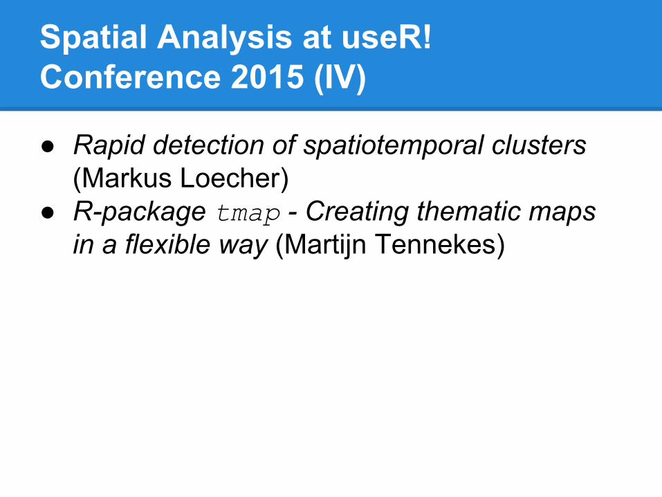
Spatial Analysis at useR! Conference 2015 (IV)
● Rapid detection of spatiotemporal clusters (Markus Loecher)
● R-package tmap - Creating thematic maps in a flexible way (Martijn Tennekes)

My personal verdict: The latest & greatest in Spatial Analysis in R

Tutorial: "Applied Spatial Data Analysis with R"
● Topics○ Why spatial data in R?○ Representing Spatial Data○ Visualizing Spatial Data○ Accessing spatial data○ Worked examples
■ Geostatistics■ Point Patterns■ Lattice Data
● Interesting but more lecture than tutorial● Slides and data available here

Tutorial: "spatstat: An R package for analysing spatial point patterns"
● Topics○ Basic statistical concepts used in spatial point
pattern analysis○ Overview of the capabilities of spatstat○ Basic analysis of a point pattern dataset
■ Calculating and plotting exploratory summaries■ Fitting Poisson, Cox, and Gibbs point process
models■ Validating and critiquing fitted models
● Didn't attend but final 20 minutes looked very promising
● Material available here (& even more here)

Keynote: "How R has changed spatial statistics"
● Excellent talk by one of the luminaries of spatial analysis, author of spatstat package
● History and collection of revolutionary ideas (past, current and future) in spatial data analysis and statistics (esp. point pattern analysis)
● Unfortunately slides not available, yet...

What’s new in igraph andnetworksGábor Csárdi
2015-07-01

About igraph
2/15

The [ operator
Imaginary adjacency matrix, queries
air['BOS', 'SFO']
#> [1] 6
CA <- c("LAX", "SFO", "SAN", "SMF", "SNA", "BUR", "OAK", "ONT", "SJC")air['BOS', CA]
#> LAX SFO SAN SMF SNA BUR OAK ONT SJC #> 7 6 1 0 0 0 0 0 1
5/15

The [ operator
Imaginary adjacency matrix, manipulation
Add an edge (and potentially set its weight):
Remove an edge:
air["BOS", "ANC"] <- TRUEair["BOS", "ANC"]
#> [1] 1
air["BOS", "ANC"] <- FALSEair["BOS", "ANC"]
#> [1] 0
6/15

The [[ operator
Imaginary adjacency list, adjacenct vertices:
air[["BOS"]]
#> $BOS#> + 269/755 vertices, named:#> [1] BGR JFK JFK JFK JFK JFK JFK JFK JFK JFK JFK JFK JFK JFK JFK#> [16] LAS LAS LAS MIA MIA EWR EWR EWR EWR EWR EWR EWR EWR EWR EWR#> [31] LAX LAX LAX LAX LAX LAX LAX PBI PBI PIT PIT PIT PIT PIT SFO#> [46] SFO SFO SFO SFO SFO IAD IAD IAD IAD IAD IAD IAD IAD IAD IAD#> [61] BDL BDL BUF BUF BUF BUF BWI BWI BWI BWI BWI BWI BWI BWI CAK#> [76] CLE CLE CLE CLE CLE CLT CLT CLT CLT CLT CLT CLT CLT CLT CMH#> [91] CMH CVG CVG CVG CVG CVG CVG CVG CVG CVG CVG DCA DCA DCA DCA#> [106] DCA DCA DCA DCA DCA DTW DTW DTW DTW DTW DTW DTW DTW DTW DTW#> [121] DTW DTW DTW GSO IND IND LGA LGA LGA LGA LGA LGA LGA LGA MDT#> [136] MKE MKE MKE MSP MSP MSP MSP MSP MSP MSY MYR ORF PHF PHL PHL#> + ... omitted several vertices
7/15

The [[ operator
Imaginary adjacency list, adjacent vertices:
air[[, "BOS"]]
#> $BOS#> + 256/755 vertices, named:#> [1] BGR JFK JFK JFK JFK JFK JFK JFK JFK JFK JFK JFK JFK LAS LAS#> [16] LAS MIA MIA MIA EWR EWR EWR EWR EWR EWR EWR EWR LAX LAX LAX#> [31] LAX LAX LAX LAX LAX PBI PBI PIT PIT PIT PIT SFO SFO SFO SFO#> [46] SFO SFO IAD IAD IAD IAD IAD IAD IAD IAD IAD BDL BDL BDL BUF#> [61] BUF BUF BUF BWI BWI BWI BWI BWI BWI CAK CAK CLE CLE CLE CLE#> [76] CLE CLE CLT CLT CLT CLT CLT CLT CLT CLT CMH CMH CVG CVG CVG#> [91] CVG CVG CVG DCA DCA DCA DCA DCA DCA DCA DCA DCA DTW DTW DTW#> [106] DTW DTW DTW DTW DTW DTW DTW DTW DTW IND IND LGA LGA LGA LGA#> [121] LGA LGA MDT MKE MKE MKE MSP MSP MSP MSP MSP MSP MSP MSP MSY#> [136] MSY MYR PHF PHL PHL PHL PHL PHL PHL PHL PHL PHL RDU RDU RDU#> + ... omitted several vertices
8/15

Pipe friendly syntax
g <- make_empty_graph(10) %>% add_vertices(5) %>% set_vertex_attr("name", value = LETTERS[1:5]) %>% add_edges(c(1,2,2,3,3,4,4,5,5,1)) %>% set_edge_attr("weight", value = runif(gsize(.)))
13/15

Easier connection to other packages
library(networkD3)d3_net <- simpleNetwork(as_data_frame(karate, what = "edges")[, 1:3])d3_net
14/15

Rapid detection of spatiotemporal clusters
Markus Loecher, Berlin School of Economics and Law
July 2nd, 2015

Spatiotemporal Clusters
Scoring unusual events in space and time has been an active andimportant field of research for decades: How do we
I distinguish normal fluctuations in a stochastic count process fromreal additive events ?
I identify spatiotemporal clusters where the event is most stronglypronounced ?
I efficiently graph these clusters in a map overlay ?
Supervised learning algorithms are proposed as an alternative to thecomputationally expensive scan statistic.The task can be reduced to detecting over-densities in space relative to abackground density.
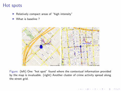
Hot spots
I Relatively compact areas of “high intensity”
I What is baseline ?
Figure: (left) One “hot spot” found where the contextual information providedby the map is invaluable. (right) Another cluster of crime activity spread alongthe street grid.

Unusual Clusters
I “Over a 5 year period there were 19 cases of a particular type of cancerreported in a town. A physician notes that there is a 1 year period thatcontains eight cases. ”
I “On Aug 17, the U.S. Army suspended all operations of the BlackHawk helicopter after the third crash in 25 days. The 3 crashes wereabout seven times the expected rate based on the previous 5 years.(S25 = 3)”
I “ Alarming number of inmate deaths in Harris County: In a 10 monthperiod, 11 inmates died at the troubled Harris County Jail, which is abouttwice the expected rate. The U.S. Department of Justice ordered the cityof Houston to pay a fine of $1000 a day until the cause was found.(S10 = 11)”

Scan Statistic
This type of spatial surveillance is computationally expensive: O(R · N4)

Unsupervised as Supervised Learning
Introduced in Hastie et al for density estimation or association rulegeneralizations. Problem must be enlarged with a simulated data set generatedby Monte Carlo techniques
-1 0 1 2
-20
24
6
•
•
•
•
•
•
•
•
•
•
••
•
•
•
•
•
•
•
•
•
••
••
•
••
•
•
•
••
•
•
•
••
•
•
•
•
•
•
•
•
•
•
•
•
•
••
••
•
•
•
•
••
••
•
•
•
••
•
•
••
•
•
•
•
•
•• ••
•
•
• ••
•
•
•
•
••
•
•
•
•
••
•
•
•
•
••
••
•
•
•
•
•
•
•
•
•
•
•
•
•
•
•
••
•
•
•
•
•
••
•
••
•
•
••
•
•
•
••
•
• ••
•
•
• •
•
•••• •••
•
•
•
•
••
•
•
•
• •
•
•
•
•••
••
•
•
••
•
•
• •
•
•
•
••
•
•
•
•
•
••
••
•
•
••
•
•
•
•
•
•
•
•
•
•
•
•
•
•
••
••
•
•
•
•
•
••
•
•
•
•
•
•
•
•
•
••
•
•
•
• •
•
••
•
•
•
•
•
•
•
•
•
•
•
••
•
•
•
•
•
•
••
•
•
•
•
•
•
•
•
•••
•
•
•
•
•
•
•
•
•
•
•
•
•
•
•
•
•
•
••
•
•
•
• •
•
•
••
•
•
•
•
••
•
•
•••
•
•
••
••
•
•
•
•
•
•
•
•
•
•
•
•
•
•
••
•
•
•
•
•
•
•
•
•
••
•
•
•
•
•
•
•
•
•
••
••
•
••
•
•
•
•
•
•
•
•
•
•
•
•
•
•
•
•
•
••
•
• •
•
•
•
•
•
•
•
•
• •
X1X1
X2
X2
FIGURE 14.3. Density estimation via classification. (Left panel:) Training setof 200 data points. (Right panel:) Training set plus 200 reference data points,generated uniformly over the rectangle containing the training data. The trainingsample was labeled as class 1, and the reference sample class 0, and a semipara-metric logistic regression model was fit to the data. Some contours for g(x) areshown.
In epidemiology cases and population naturally provide two classes, for anomalydetection the background ”population” is taken to be some sort of average.

CART
A cluster found by a classification tree visualized on a Google map tile. Thenumeric labels indicate the fraction of the positive class labels.

TreeHotspots
R package with new functionalities
I Rotation of Data
I Visualization of selected leaves
I Overlay on maps (Google and OSM)
I User written splitting functions for rpart:I Baseline Distributions eliminate need for point augmentationI SatScan Poisson and Binomial Likelihood, e.g.(
c
E [c]
)c
·(
C − c
C − E [c]
)C−c

Simulations

Simulations

SF crime data, on map
Figure: positive class is given by (left) drug crimes and (right) robbery relatedincidents.

Martijn Tennekes
R-package tmap Creating thematic maps in a flexible way

= Thematic map
Thematic map
3

Layered approach
4
Defaults • Data • Aesthetics
Coordinates
Scales
Layers • Data • Aesthetics • Geometry • Statistics • Position
Facets
Shape specification • Spatial object
Types: ◊ Polygons • Points ⁄ Lines # Raster
Data • Map projection • Bounding box
Layers • Aesthetics • Statistics • Scale
A Layered Grammar of Graphics (Wickham, 2010) Implemented in ggplot2
Facets
Layered approach in tmap
Group
1
1 or more

tm_fill()
Building a thematic map
5
tm_shape(NLD_muni, projection=“rd”) +

tm_fill(“blue”)
tm_shape(NLD_muni, projection=“rd”) +
Building a thematic map
6
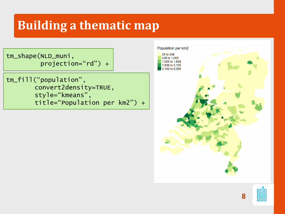
Building a thematic map
8
tm_shape(NLD_muni, projection=“rd”) +
tm_fill(“population”, convert2density=TRUE, style=“kmeans”, title=“Population per km2”) +

Building a thematic map
9
tm_shape(NLD_muni, projection=“rd”) +
tm_fill(“population”, convert2density=TRUE, style=“kmeans”, title=“Population per km2”) +
tm_borders(alpha=.5) +

Building a thematic map
10
tm_shape(NLD_muni, projection=“rd”) +
tm_fill(“population”, convert2density=TRUE, style=“kmeans”, title=“Population per km2”) +
tm_borders(alpha=.5) +
tm_shape(NLD_prov) +
tm_borders(lwd=2) +
tm_text(“name”, size=.8, shadow=TRUE, bg.color="white", bg.alpha=.25)

Quick thematic map
11 qtm(NLD_muni)
qtm(NLD_muni, fill="population", convert2density=TRUE)
qtm(NLD_muni, fill="population", convert2density=TRUE, fill.style="kmeans", fill.title="Population per km2") + qtm(NLD_prov, fill=NULL, text="name", text.size=.7, borders.lwd=2, text.bg.color="white", text.bg.alpha=.25, shadow=TRUE)
• Quick thematic map: qtm • Wrapper for the main plotting method

tmap and the field
15
tmap
sp
rgdal grid
ggplot2 (+ggmap)
rgeos
sp
base graphics
Plotting thematic maps:
+ Grammar of graphics + Familiar syntax - Processing required: - Shape to be fortified - Layout to be polished
+ Familiar syntax - Do-it-yourself!
+ Easy to use + Flexible + Layer based + OSM + Small multiples - New syntax - Not interactive (yet)
rworldmap
raster RColorBrewer
classInt
GIStools choroplethr
+ Less DIY work - New syntax - Limited possibilities
maps
osmar
OpenStreetMap javascript
(leaflet library)
+ Interactive + Flexible + Layered based + OSM - Small multiples - New syntax * Lower level (w.r.t. tmap)
leaflet
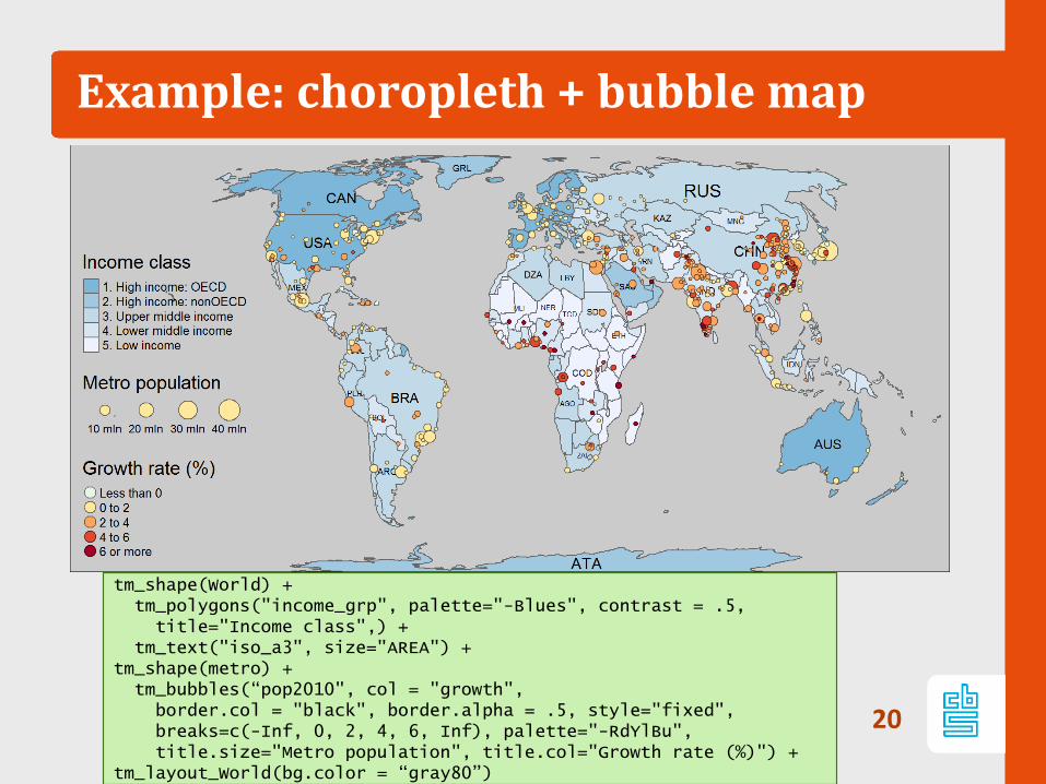
Example: choropleth + bubble map
20
tm_shape(World) + tm_polygons("income_grp", palette="-Blues", contrast = .5, title="Income class",) + tm_text("iso_a3", size="AREA") + tm_shape(metro) + tm_bubbles(“pop2010", col = "growth", border.col = "black", border.alpha = .5, style="fixed", breaks=c(-Inf, 0, 2, 4, 6, Inf), palette="-RdYlBu", title.size="Metro population", title.col="Growth rate (%)") + tm_layout_World(bg.color = “gray80”)
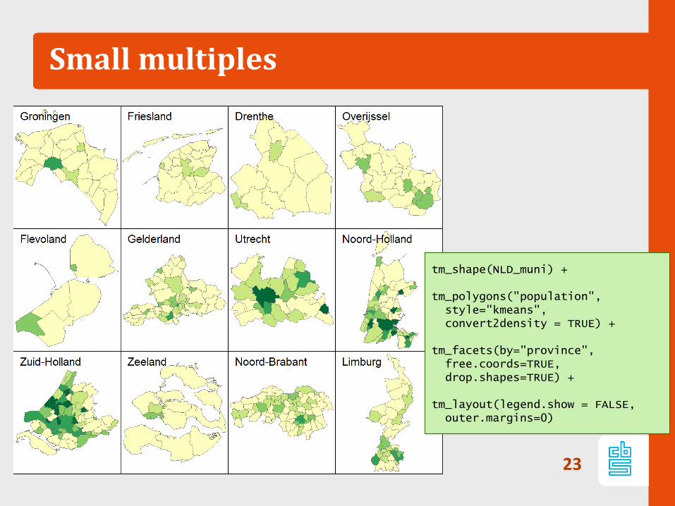
Small multiples
23
tm_shape(NLD_muni) + tm_polygons("population", style="kmeans", convert2density = TRUE) + tm_facets(by="province", free.coords=TRUE, drop.shapes=TRUE) + tm_layout(legend.show = FALSE, outer.margins=0)

Histogram
24
tm_shape(NLD_muni, projection="rd") + tm_borders(alpha = .5) + tm_fill("population", convert2density = TRUE, style= "kmeans", title="Population per km2", legend.hist = TRUE) + tm_shape(NLD_prov) + tm_borders(lwd=2) + tm_text("name", size=0.8, shadow=TRUE, bg.color="white", bg.alpha=.25) + tm_layout(draw.frame=FALSE, bg.color="white", inner.margins=c(.02, .05, .02, .02), legend.hist.bg.color = "grey85")

Overall a great conference