IN-NETWORK PROCESSING FOR MISSION-CRITICAL WIRELESS ...cpslab.cs.mcgill.ca/people/qiaoxiang/files/papers/dissertation14-Qiao-Xiang.pdf · in-network processing for mission-critical

IN-NETWORK PROCESSING FORMISSION-CRITICALWIRELESSNETWORKED SENSING AND CONTROL: A REAL-TIME, EFFICIENCY, AND

RESILIENCY PERSPECTIVE

by

QIAO XIANG

DISSERTATION

Submitted to the Graduate School

of Wayne State University,

Detroit, Michigan

in partial fulfillment of the requirements

for the degree of

DOCTOR OF PHILOSOPHY

2014

MAJOR: COMPUTER SCIENCE

Approved by:

Advisor Date

c© COPYRIGHT BY

QIAO XIANG

2014

All Rights Reserved

DEDICATION

To my family and friends

ii

iv

TABLE OF CONTENTS

Dedication . . . . . . . . . . . . . . . . . . . . . . . . . . . . . . . . . . . . . . . . . . . . . . . . . . . . . . . . . . . . . . . . . . . ii

Acknowledgments . . . . . . . . . . . . . . . . . . . . . . . . . . . . . . . . . . . . . . . . . . . . . . . . . . . . . . . . . . . . iii

List of Tables . . . . . . . . . . . . . . . . . . . . . . . . . . . . . . . . . . . . . . . . . . . . . . . . . . . . . . . . . . . . . . . . vii

List of Figures . . . . . . . . . . . . . . . . . . . . . . . . . . . . . . . . . . . . . . . . . . . . . . . . . . . . . . . . . . . . . . . viii

Chapter 1 Introduction . . . . . . . . . . . . . . . . . . . . . . . . . . . . . . . . . . . . . . . . . . . . . . . . . . . . . . . . 1

Contribution of this dissertation . . . . . . . . . . . . . . . . . . . . . . . . . . . . . . . . . . . . . . . . . . . . . . . . 2

Organization of this dissertation . . . . . . . . . . . . . . . . . . . . . . . . . . . . . . . . . . . . . . . . . . . . . . . 3

Chapter 2 Real-time packet packing scheduling . . . . . . . . . . . . . . . . . . . . . . . . . . . . . . . . . . . . 4

Preliminary . . . . . . . . . . . . . . . . . . . . . . . . . . . . . . . . . . . . . . . . . . . . . . . . . . . . . . . . . . . . . . . 4

Motivation for packing . . . . . . . . . . . . . . . . . . . . . . . . . . . . . . . . . . . . . . . . . . . . . . . . . . . . . 7

System model and problem definition . . . . . . . . . . . . . . . . . . . . . . . . . . . . . . . . . . . . . . . . . 11

System Model . . . . . . . . . . . . . . . . . . . . . . . . . . . . . . . . . . . . . . . . . . . . . . . . . . . . . . . 11

Problem Definition . . . . . . . . . . . . . . . . . . . . . . . . . . . . . . . . . . . . . . . . . . . . . . . . . . . . 12

Complexity of joint optimization . . . . . . . . . . . . . . . . . . . . . . . . . . . . . . . . . . . . . . . . . . . . . 12

Complexity when K 3 . . . . . . . . . . . . . . . . . . . . . . . . . . . . . . . . . . . . . . . . . . . . . . . 13

Complexity when K = 2 . . . . . . . . . . . . . . . . . . . . . . . . . . . . . . . . . . . . . . . . . . . . . . . . 23

A Utility-based online algorithm . . . . . . . . . . . . . . . . . . . . . . . . . . . . . . . . . . . . . . . . . . . . . 34

Utility calculation . . . . . . . . . . . . . . . . . . . . . . . . . . . . . . . . . . . . . . . . . . . . . . . . . . . . . 35

Scheduling rule . . . . . . . . . . . . . . . . . . . . . . . . . . . . . . . . . . . . . . . . . . . . . . . . . . . . . . 39

Competitive analysis . . . . . . . . . . . . . . . . . . . . . . . . . . . . . . . . . . . . . . . . . . . . . . . . . . 39

Implementation . . . . . . . . . . . . . . . . . . . . . . . . . . . . . . . . . . . . . . . . . . . . . . . . . . . . . . 42

Performance evaluation . . . . . . . . . . . . . . . . . . . . . . . . . . . . . . . . . . . . . . . . . . . . . . . . . . . . 43

Methodology . . . . . . . . . . . . . . . . . . . . . . . . . . . . . . . . . . . . . . . . . . . . . . . . . . . . . . . . 44

Measurement Results . . . . . . . . . . . . . . . . . . . . . . . . . . . . . . . . . . . . . . . . . . . . . . . . . . 47

v

Related work . . . . . . . . . . . . . . . . . . . . . . . . . . . . . . . . . . . . . . . . . . . . . . . . . . . . . . . . . . . . . 59

Concluding remarks . . . . . . . . . . . . . . . . . . . . . . . . . . . . . . . . . . . . . . . . . . . . . . . . . . . . . . . 64

Chapter 3 Energy-efficient network coding based routing . . . . . . . . . . . . . . . . . . . . . . . . . . 66

Preliminary . . . . . . . . . . . . . . . . . . . . . . . . . . . . . . . . . . . . . . . . . . . . . . . . . . . . . . . . . . . . . . 66

System settings and problem definition . . . . . . . . . . . . . . . . . . . . . . . . . . . . . . . . . . . . . . . . 67

System settings . . . . . . . . . . . . . . . . . . . . . . . . . . . . . . . . . . . . . . . . . . . . . . . . . . . . . . 68

Comparison between inter-flow and intra-flow network coding . . . . . . . . . . . . . . . . . 68

Problem definition . . . . . . . . . . . . . . . . . . . . . . . . . . . . . . . . . . . . . . . . . . . . . . . . . . . . 69

Cost optimization for NC-based routing . . . . . . . . . . . . . . . . . . . . . . . . . . . . . . . . . . . . . . . . 70

Effective load based assignment algorithm for Q1 . . . . . . . . . . . . . . . . . . . . . . . . . . . 70

Optimal NC-based transmission cost algorithm . . . . . . . . . . . . . . . . . . . . . . . . . . . . . 74

A theoretical comparison with other routing protocols . . . . . . . . . . . . . . . . . . . . . . . . 79

Protocol design and implementation . . . . . . . . . . . . . . . . . . . . . . . . . . . . . . . . . . . . . . . . . . . 83

Routing engine . . . . . . . . . . . . . . . . . . . . . . . . . . . . . . . . . . . . . . . . . . . . . . . . . . . . . . . 84

Modified NSB coded feedback . . . . . . . . . . . . . . . . . . . . . . . . . . . . . . . . . . . . . . . . . . 84

Rate control . . . . . . . . . . . . . . . . . . . . . . . . . . . . . . . . . . . . . . . . . . . . . . . . . . . . . . . . . 87


Methodology . . . . . . . . . . . . . . . . . . . . . . . . . . . . . . . . . . . . . . . . . . . . . . . . . . . . . . . . 88

Measurement Results . . . . . . . . . . . . . . . . . . . . . . . . . . . . . . . . . . . . . . . . . . . . . . . . . . 90

Related work . . . . . . . . . . . . . . . . . . . . . . . . . . . . . . . . . . . . . . . . . . . . . . . . . . . . . . . . . . . . . 95

Network-coding-based multicast . . . . . . . . . . . . . . . . . . . . . . . . . . . . . . . . . . . . . . . . . 97

Network-coding-based opportunistic routing . . . . . . . . . . . . . . . . . . . . . . . . . . . . . . . 99


Chapter 4 Proactive network coding based protection . . . . . . . . . . . . . . . . . . . . . . . . . . . . 103

Preliminary . . . . . . . . . . . . . . . . . . . . . . . . . . . . . . . . . . . . . . . . . . . . . . . . . . . . . . . . . . . . . . 103

vi

System model and problem definition . . . . . . . . . . . . . . . . . . . . . . . . . . . . . . . . . . . . . . . . . 105

1+1 NC-based proactive protection problem . . . . . . . . . . . . . . . . . . . . . . . . . . . . . . . . . . . . 106

Complexity study on problem Q . . . . . . . . . . . . . . . . . . . . . . . . . . . . . . . . . . . . . . . . 106

A finding in the NP-hardness proof for two-commodity integral flow problem . . . . 109

A heuristic algorithm for Problem Q . . . . . . . . . . . . . . . . . . . . . . . . . . . . . . . . . . . . . . . . . . 111

Protocol design and implementation . . . . . . . . . . . . . . . . . . . . . . . . . . . . . . . . . . . . . . . . . . 113


Methodology . . . . . . . . . . . . . . . . . . . . . . . . . . . . . . . . . . . . . . . . . . . . . . . . . . . . . . . 114

Measurement Results . . . . . . . . . . . . . . . . . . . . . . . . . . . . . . . . . . . . . . . . . . . . . . . . . 117

Related work . . . . . . . . . . . . . . . . . . . . . . . . . . . . . . . . . . . . . . . . . . . . . . . . . . . . . . . . . . . . 122


Chapter 5 Conclusion . . . . . . . . . . . . . . . . . . . . . . . . . . . . . . . . . . . . . . . . . . . . . . . . . . . . . . . 126

References . . . . . . . . . . . . . . . . . . . . . . . . . . . . . . . . . . . . . . . . . . . . . . . . . . . . . . . . . . . . . . . . . 127

Abstract . . . . . . . . . . . . . . . . . . . . . . . . . . . . . . . . . . . . . . . . . . . . . . . . . . . . . . . . . . . . . . . . . . . 135

Autobiographical Statement . . . . . . . . . . . . . . . . . . . . . . . . . . . . . . . . . . . . . . . . . . . . . . . . . . . . 137

LIST OF TABLES

Table 1 Notations used in Chapter 2 . . . . . . . . . . . . . . . . . . . . . . . . 6

vii

LIST OF FIGURES

Figure 1 Rk =AC1

ACk. . . . . . . . . . . . . . . . . . . . . . . . . . . . . . . . . 9

Figure 2 K∗ when l1 = 12, h = 0.375, and Kmax = 100. . . . . . . . . . . . . . 10

Figure 3 ACK when l1 = 12, h = 0.375, and Kmax = 100. . . . . . . . . . . . . 10

Figure 4 A tree with n+ 2 nodes . . . . . . . . . . . . . . . . . . . . . . . . . . 13

Figure 5 Reduction from SAT to P0 when K ≥ 3 . . . . . . . . . . . . . . . . . 14

Figure 6 Lifetimes of information elements . . . . . . . . . . . . . . . . . . . . 15

Figure 7 Example of optimal packing when K ≥ 3 . . . . . . . . . . . . . . . . 17

Figure 8 Deriving optimal packing scheme from SAT assignment whenK ≥ 3 . . 18

Figure 9 Reduction from SAT to P0 when K = 2 . . . . . . . . . . . . . . . . . 25

Figure 10 Deriving optimal packing scheme from SAT assignment whenK = 2 . . 27

Figure 11 NetEye wireless sensor network testbed . . . . . . . . . . . . . . . . . . 44

Figure 12 Packing ratio: D3 . . . . . . . . . . . . . . . . . . . . . . . . . . . . . 47

Figure 13 Delivery reliability: D3 . . . . . . . . . . . . . . . . . . . . . . . . . . 48

Figure 14 Delivery cost: D3 . . . . . . . . . . . . . . . . . . . . . . . . . . . . . 48

Figure 15 Deadline catching ratio: D3 . . . . . . . . . . . . . . . . . . . . . . . . 49

Figure 16 Latency jitter: D3 . . . . . . . . . . . . . . . . . . . . . . . . . . . . . 49

Figure 17 Histogram of routing hop count: D3 with maximum latency L1 . . . . . 50










viii


Figure 28 Link reliability: D6 . . . . . . . . . . . . . . . . . . . . . . . . . . . . 58

Figure 29 Histogram of routing hop count: D6 with maximum latency L1 . . . . . 58

Figure 30 Per-element delivery cost vs. geo-distance: D6 with maximum latency L1 59

Figure 31 Packing ratio: Elites . . . . . . . . . . . . . . . . . . . . . . . . . . . . 60

Figure 32 Delivery reliability: Elites . . . . . . . . . . . . . . . . . . . . . . . . . 60

Figure 33 Delivery cost: Elites . . . . . . . . . . . . . . . . . . . . . . . . . . . . 61

Figure 34 Deadline catching ratio: Elites . . . . . . . . . . . . . . . . . . . . . . . 61

Figure 35 Latency jitter: Elites . . . . . . . . . . . . . . . . . . . . . . . . . . . . 62

Figure 36 An illustrating example of NC-based routing . . . . . . . . . . . . . . . 71

Figure 37 Example topology . . . . . . . . . . . . . . . . . . . . . . . . . . . . . 72

Figure 38 Routing braid v.s. single path routing . . . . . . . . . . . . . . . . . . . 81

Figure 39 Delivery reliability: 10 sources . . . . . . . . . . . . . . . . . . . . . . 91

Figure 40 Delivery cost: 10 sources . . . . . . . . . . . . . . . . . . . . . . . . . 91

Figure 41 Goodput: 10 sources . . . . . . . . . . . . . . . . . . . . . . . . . . . . 92

Figure 42 Routing diversity: 10 sources . . . . . . . . . . . . . . . . . . . . . . . 93

Figure 43 Delivery reliability: 20 sources . . . . . . . . . . . . . . . . . . . . . . 94

Figure 44 Delivery cost: 20 sources . . . . . . . . . . . . . . . . . . . . . . . . . 94

Figure 45 Goodput: 20 sources . . . . . . . . . . . . . . . . . . . . . . . . . . . . 95

Figure 46 Routing diversity: 20 sources . . . . . . . . . . . . . . . . . . . . . . . 96

Figure 47 lobe i for variable xi . . . . . . . . . . . . . . . . . . . . . . . . . . . . 110

Figure 48 lobe i for variable xi . . . . . . . . . . . . . . . . . . . . . . . . . . . . 110

Figure 49 Delivery reliability: 10 sources without failure . . . . . . . . . . . . . . 118

Figure 50 Delivery cost: 10 sources without failure . . . . . . . . . . . . . . . . . 118

Figure 51 Goodput: 10 sources without failure . . . . . . . . . . . . . . . . . . . 119

Figure 52 Delivery reliability: 10 sources with failures . . . . . . . . . . . . . . . 120

Figure 53 Delivery cost: 10 sources with failures . . . . . . . . . . . . . . . . . . 120

Figure 54 Goodput: 10 sources with failures . . . . . . . . . . . . . . . . . . . . . 121

ix

1

CHAPTER 1

INTRODUCTION

After the past decade of active research and field trials, wireless sensor networks (which

we call sensornets interchangeably) have started penetrating into many areas of science, engi-

neering, and our daily life. They are also envisioned to be an integral part of cyber-physical

systems such as those for alternative energy, transportation, and healthcare. In supporting

mission-critical, real-time, closed loop sensing and control, CPS sensornets represent a sig-

nificant departure from traditional sensornets which usually focus on open-loop sensing, and it

is critical to ensure messaging quality (e.g., timeliness of data delivery) in CPS sensornets. The

stringent application requirements in CPS make it necessary to rethink about sensornet design,

and one such problem is in-network processing.

For resource constrained sensornets, in-network processing (INP) improves energy effi-

ciency and data delivery performance by reducing network traffic load and thus channel con-

tention. Over the past years, many INP methods have been proposed for query processing

[54, 69, 58, 15] and general data collection [20, 21, 43, 52, 61, 71]. Not focusing on mission-

critical WCPS, however, these works have mostly ignored the Quality of Services constraints

when designing INP mechanisms. Thus, the interaction between specific, real-world INP meth-

ods and QoS of data delivery remains a largely unexplored issue in WCPS systems. This is an

important issue because

1. It affects the efficiency and quality of real-time, efficient and resilient embedded sensing

and control;

2. As we will show later in this dissertation, different INP methods and their different con-

straints (e.g., aggregation capacity limit and re-aggregation tolerance) affect, to a greater

extent than network and traffic properties, the complexity and the protocol design in

jointly optimizing in-network processing and QoS of data delivery.

In this dissertation, we focus on two widely used INP methods, packet packing and network

coding (which we use NC interchangeably hereafter), and their quality of services in mission-

2

critical wireless networked sensing and control. Our results show that these two techniques

can significantly improve network performance in terms of timeliness of data delivery, energy

efficiency, delivery reliability and network throughput under stringent application QoS require-

ments in WCPS. More specifically, we study the joint optimization problem of packet packing

and real-time constraints of data delivery, the minimal cost network-coding-based (NC-based)

routing problem, and proactive NC- based protection problem for mission-critical WCPS.

Contribution of this dissertation

Before presenting all the details, we first summarize the contribution of this dissertation as

follows:

1. We examine the complexity and impact of jointly optimizing packet packing and the

timeliness of data delivery. We find that different packing constraints have a large effect

on the problem complexity. We identify conditions for the joint optimization to be strong

NP-hard and conditions for it to be solvable in polynomial time. We also develop a

local, distributed online protocol tPack for maximizing the local utility of each node,

and we prove the competitiveness of the protocol with respect to optimal solutions. Our

measurement study on the NetEye testbed demonstrates the importance of QoS- and

aggregation constraint aware optimization of packet packing.

2. We study the transmission cost minimization problem of network coding based routing.

We propose the first mathematical framework to compute the transmission cost of NC-

based routing. We then find that this minimization problem is polynomial solvable and

designed an greedy optimal algorithm. We prove the optimality of this algorithm and

conduct a theoretical comparison between our minimal cost NC-based routing and tradi-

tional single path routing. We show that not only the shortest single path routing is not

necessarily selected into the optimal routing braid, but also that the optimal routing braid

has a transmission cost upper bounded by the shortest single path routing. We develop

a distributed NC-based routing protocol EENCR to implement this optimal algorithm.

3

EENCR inherits the advantages of both single path routing protocol and network coding

based opportunistic routing protocol. Our measurement study on the NetEye in a new

environment show that EENCR outperforms a state-of-the art single path routing proto-

col and two other classic network coding based opportunistic routing protocols in terms

of reliability, delivery cost and goodput.

3. Based on our findings in the minimal cost NC-based routing, we also study the 1+1 proac-

tive network coding based protection problem. We prove that finding 2 node-disjoint

routing braids with minimal transmission cost for NC-based transmission is NP-hard

even under a simple setting. We then propose a heuristic yet efficient algorithm to con-

struct 2 node-disjoint routing braids by fully exploring the routing diversity in the net-

work. We develop a proactive network coding protection protocol ProNCP to evaluate

this algorithm. Experiment results show that ProNCP is resilient to various random tran-

sient node failures in wireless networked sensing and control systems by providing a

close to 100% delivery reliability and incurring only a 50% transmission cost compared

with the classic 2 shortest node-disjoint path algorithm.

Organization of this dissertation

The rest of this dissertation is organized as follows. In Chapter 2 we present our study

on joint optimization between packet packing and real-time constraints of data delivery. In

Chapter 3, we study the energy-efficient NC-based routing problem. We then study the 1+1

proactive NC-based protection problem in Chapter 4. We conclude this dissertation in Chapter

5.

4

CHAPTER 2

REAL-TIME PACKET PACKING SCHEDULING

Preliminary

Towards understanding the interaction between INP and data delivery latency in foresee-

able real-world sensornet deployments, we focus on a widely used, application-independent

INP method — packet packing where multiple short packets are aggregated into a single long

packet [29, 53]. In sensornets (especially those for real-time sensing and control), an informa-

tion element from each sensor is usually short, for instance, less than 10 bytes [9, 54]. Yet the

header overhead of each packet is relatively high in most sensornet platforms, for instance, up

to 31 bytes at the MAC layer alone in IEEE 802.15.4 based networks. It is also expected that

more header overhead will be introduced at other layers (e.g., routing layer) as we standardize

sensornet protocols such as in the effort of the IETF working groups 6LowPAN [4] and ROLL

[33]. Besides header overhead, MAC coordination also introduces non-negligible overhead

in wireless networks [53]. If we only transmit one short information element in each packet

transmission, the high overhead in packet transmission will significantly reduce the network

throughput; this is especially the case for high speed wireless networks such as IEEE 802.15.4a

ultrawideband (UWB) networks. Fortunately, the maximum size of packet payload is usually

much longer than that of each information element, for instance, 128 bytes per MAC frame in

802.15.4. Therefore, we can aggregate multiple information elements into a single packet to

reduce the amortized overhead of transmitting each element. Packet packing also reduces the

number of packets contending for channel access, hence it reduces the probability of packet

collision and improves information delivery reliability, as we will show in Chapter . The ben-

efits of packet packing have also been recognized by the IETF working groups 6LowPAN and

ROLL.

Unlike total aggregation assumed in [10] and [59], the number of information elements that

can be aggregated into a single packet is constrained by the maximum packet size, thus we have

to carefully schedule information element transmissions so that the degree of packet packing

5

(i.e., the amount of sensing data contained in packets) can be maximized without violating

application requirement on the timeliness of data delivery. As a first step toward understanding

the complexity of jointly optimizing INP and QoS with aggregation constraints, we analyze the

impact that aggregation constraints have on the computational complexity of the problem, and

we prove the following:

1. When a packet can aggregate three or more information elements, the problem is strong

NP-hard, and there is no polynomial-time approximation scheme (PTAS).

2. When a packet can only aggregate two information elements, the complexity depends on

whether two elements in a packet can be separated and re-packed with other elements on

their way to the sink: if the elements in a packet can be separated, the problem is strong

NP-hard and there is no PTAS for the problem; otherwise it can be solved in polynomial

time by modeling the problem as a maximum weighted matching problem in an interval

graph.

3. The above conclusions hold whether or not the routing structure is a tree or a linear chain,

and whether or not the information elements are of equal length.

Besides shedding light on the complexity and protocol design of jointly optimizing data deliv-

ery timeliness and packet packing (as well as other INP methods), these findings incidentally

answer several open questions on the complexity of batch-process scheduling in interval graphs

[22].

To understand the impact of jointly optimizing packet packing and data delivery timeliness,

we design a distributed, online protocol tPack that schedules packet transmissions to maxi-

mize the local utility of packet packing at each node while taking into account the aggregation

constraint imposed by the maximum packet size. Using a testbed of 130 TelosB motes, we

experimentally evaluate the properties of tPack. We find that jointly optimizing data delivery

timeliness and packet packing and considering real-world aggregation constraints significantly

improve network performance (e.g. in terms of high reliability, high energy efficiency, and low

delay jitter).

6

Table 1: Notations used in Chapter 2

Common notationsK maximum number of information elements al-

lowed in a packetETXvivj (l) expected number of transmissions taken to suc-

cessfully deliver a packet of length l along link(vi, vj)

tvivk(l) maximum time taken to deliver a packet oflength l from vi to vk in the absence of packetpacking and packing-oriented scheduling

Notations used in the section of preliminary study onlyR root of a directed collection treex an information elementvx the node where x is generatedlx length of xrx time when x is generateddx deadline of delivering x to Rsx spare time in delivering x

[rx, dx] lifetime of xNotations used in the section of complexity study onlyn number of variables in a SAT instancem number of clauses in a SAT instanceXj jth variable of a SAT instanceCi ith clause of a SAT instancexji information element corresponding to the vari-

able Xj in a clause Ci

[rji , dji ] lifetime of xj

i

axjk kth auxiliary information element for variable

Xj

[rjaxk, djaxk

] lifetime of axjk

zi information element generated by node vci[ri, di] lifetime of zit1 transmission time from any leaf node to its par-

entt2 transmission time from any node vj to node vt3 transmission time from node v to node st4 transmission time from any node vci to node v

The rest of this chapter is organized as follows. We first analyze the benefits of packet

packing in lossy wireless networks in We then discuss the system model and precisely define

7

the joint optimization problem in. Next we analyze the complexity of the problem in under dif-

ferent settings, and present the tPack protocol to provide a distributed solution to this problem.

After presenting the protocol design and implementation details, we experimentally evaluate

the performance of tPack and study the impact of packet packing as well as joint optimization.

We discuss related work before concluding this study in the end of this chapter. For conve-

nience, we summarize in Table 1 the notations used in the section of preliminary study and the

section of complexity study.

Motivation for packing

While aggregating short information elements reduces the overhead of transmitting each

information element, it increases the length of packets being transmitted. Given that packet

delivery rate of a wireless link decreases as packet length increases, a longer packet with aggre-

gated information elements may be retransmitted more often, for reliable data delivery, than the

shorter packets without aggregation. To understand whether packet packing is still beneficial

in the presence of lossy wireless links, therefore, we need to understand whether the increased

packet loss rate overshadows the benefits of packet packing. To this end, we mathematically

analyze the issue as follows.

For simplicity, we assume in this section that the status (i.e., success or failure) of different

packet transmissions are independent, and we corroborate the analytical results through testbed

based measurement in later sections where temporal link correlation exists. For convenience,

we define the following notations:

l1 : payload length of an unpacked packet, i.e., the length of a single infor-

mation element;

p1 : delivery rate of an unpacked packet;

k : packing ratio, i.e., the ratio of the payload length of a packed packet to

that of an unpacked packet;

h : the ratio of header length to payload length in an unpacked packet.

8

Then, for a packed packet with packing ratio k, the ratio of the overall length of the packed

packet to that of an unpacked packet is kl1+hl1l1+hl1

. Thus, the delivery rate pk of the packed packet

can be calculated as follows:

pk = pkl1+hl1l1+hl1

1 = pk+h1+h

1

To reflect the overhead of transmitting a packet pkt over a wireless link, we define the

amortized cost (AC) of transmitting pkt as follows:

ACpkt =ETXpkt

lenpkt

(1)

where lenpkt is the payload length of pkt, and ETXpkt is the expected number of transmissions

taken to successfully deliver pkt over the wireless link. Given that the expected number of

transmissions to successfully deliver a packet with packing ratio k is 1pk, the amortized cost of

transmitting a packet with packing ratio k, denoted by ACk, can be calculated as follows:

ACk =1/pkkl1

=1

kl1pk(2)

Since an unpacked packet has a packing ratio of 1, the amortized cost of transmitting an

unpacked packet is AC1, that is, 1l1p1.

For a given packing ratio k, the ratio Rk of AC1 to ACk reflects whether packet packing is

beneficial, that is, packet packing is beneficial ifRk > 1. Precisely,Rk is calculated as follows:

Rk =AC1

ACk

= kpk−1

1+h

1 (3)

In a typical sensornet system [9, 8], the ratio h of header length to that of a single informa-

tion element is around 3, and the packing ratio can be up to 12. For h = 3, Figure 1 shows Rk

as a function of p1 and k, when h = 3. From the figure, we can see that packet packing reduces

the amortized cost of packet transmission as long as the link reliability is no less than 40%,

which is usually the case in practice (e.g., link reliability was ∼75% even in heavily loaded

sensornet systems [9, 8]). We also see that, if link reliability is greater than 67%, the amortized

9

0.1 0.2 0.3 0.4 0.5 0.6 0.7 0.8 0.90

2

4

6

8

10

12

p1

Rk

k = 3k = 6k = 9k = 12reference (Rk = 1)

Figure 1: Rk = AC1

ACk

cost of packet transmission always decreases as the packing ratio increases. Since link reliabil-

ity is usually greater than 67% in practice, we can always try to maximize the packing ratio so

that the amortized cost of packet transmission is reduced.

Denoting k∗ as the optimal packing ratio that minimize the amortized cost for transmitting

a packet, we then study the relationship between k∗ and p1. From Equation 2, we have:

ACk =1

kl1pk=

1

kl1pk+h1+h

1

(4)

To minimize ACk, we need to maximize f(k) = kl1pk+h1+h

1 . When k ∈ R+, f(k) is a convex

function. Let f ′(k) = 0. we have k∗R = 1+h

ln p−1

1

. Therefore, when k ∈ N+, k∗ is calculated as

follows:

k∗ = argmink∈{1,�k∗R�,�k∗

R�}{ACk} (5)

In Figure 2, k∗ increases as the link reliability increases. When p1 is greater than 75%, k∗

increase faster, which implies that packet packing can bring more benefit on amortized cost

when link reliability is high. Figure 3 shows the relationship between ACk and k when p1 =

0.9. From the figure we can find that it is not always beneficial to pack as many small packets

as possible. There exists a threshold on the packing ratio. When k exceeds this threshold, the

amortized cost will increase. This motivates us to explore how to perform packing at each node

10

0 0.2 0.4 0.6 0.8 10

20

40

60

80K

*

p1

Figure 2: K∗ when l1 = 12, h = 0.375, and Kmax = 100.

0 20 40 60 80 10010−2

10−1

100

101

AC

k

K

Figure 3: ACK when l1 = 12, h = 0.375, andKmax = 100.

11

in the network.

Remarks: The above analysis focuses on a single link, but the observations easily carry

over to multi-hop networks since link reliability p1 reflects the impact of channel fading and

collision even in the case of multi-hop networks.1 The analysis has not considered the benefits

(e.g., fewer number of packet collisions) of reduced channel contention as a result of packet

packing (which reduces the number of packets contending for channel access). We will study

the impact of these factors through testbed based measurement in the performance evaluation

section.

System model and problem definition

Having verified the benefits of packet packing in lossy wireless networks in last section, we

now discuss the system model and define the joint optimization problems we will focus on in

this paper.

System Model

We consider a directed collection tree T = (V,E), where V and E are the set of nodes and

edges in the tree. V = {vi : i = 1 . . .N} ∪ {R} where R is the root of the tree and representsthe data sink of a sensornet, and {vi : i = 1 . . . N} are the set ofN sensor nodes in the network.

An edge 〈vi, vj〉 ∈ E if vj is the parent of vi in the collection tree. The parent of a node vi in T

is denoted as pi. We use ETXvivj (l) to denote the expected number of transmissions required

for delivering a packet of length l from a node vi to its ancestor vj , and we use tvivk(l) to denote

the maximum time taken to deliver a packet of length l from vi to vk in the absence of packet

packing and packing-oriented scheduling.

Each information element x generated in the tree is identified by a 4-tuple (vx, lx, rx, dx)

where vx is the node that generates x, lx is the length of x, rx is the time when x is generated,

and dx is the deadline by which x needs to be delivered to the sink node R. We use sx =

1Note that the increased per-packet transmission time as a result of increased packet length will not causemore collision, since the time taken to transmit a packet (e.g., ∼ 4 milliseconds) is usually much less than theinter-packet interval (e.g., usually at least a few seconds).

12

dx − (rx + tvxR(lx)) to denote the spare time for x, and we define the lifetime of x as [rx, dx].

Problem Definition

Given a collection tree T and a set of information elements X = {x} generated in the tree,we define the problem of jointly optimizing packet packing and the timeliness of data delivery

as follows:

Problem P: given T and X , schedule the transmission of each element inX to minimize the

total number of packet transmissions required for delivering X to the sink R while ensuring

that each element be delivered to R before its deadline.

In an application-specific sensornet, the information elements generated by different nodes

depend on the application but may well be of equal length [9]. Depending on whether the sen-

sornet is designed for event detection or data collection, moreover, the information elementsX

may follow certain arrival processes. Based on the specific arrival process of X , the following

special cases of problem P tend to be of practical relevance in particular:

Problem P0: same as P except that 1) the elements of X are of equal length, and 2) X

includes at most one element from each node; this problem can represent sensornets that detect

rare events.

Problem P1: same as P except that 1) the elements of X are of equal length, and 2) every

two consecutive elements generated by the same node vi are separated by a time interval whose

length is randomly distributed in [a, b]; this problem can represent periodic data collection

sensornets (with possible random perturbation to the period).

Problem P2: same as P except that the elements of X are of equal length; this problem

represents general application-specific sensornets.

Complexity of joint optimization

The complexity of problem P depends on aggregation constraints such as maximum packet

size and whether information elements in a packet can be separated and repacked with other

elements. For convenience, we useK to denote the maximum number of information elements

13

that can be packed into a single packet. (Note thatK depends on the maximum packet size and

the lengths of information elements in problem P.) In what follows, we first analyze the case

whenK ≥ 3 and then the case whenK = 2, and we discuss how aggregation constraints affect

the problem complexity.

Complexity when K ≥ 3

We first analyze the complexity and the hardness of approximation for problem P0, then

we derive the complexity of P1, P2, and P accordingly. The analysis is based on reducing the

Boolean-satisfiability-problem (SAT) [26] to P0 as we show below.

Theorem 1 When K ≥ 3, problem P0 is strong NP-hard whether or not the routing structure

is a tree or a linear chain.

Proof To prove that P0 is strong NP-hard, we first present a polynomial transformation f from

the SAT problem to P0, then we prove that an instance Π of SAT is satisfiable if and only if the

optimal solution of Π′ = f(Π) has certain minimum number of transmissions.

Given an instance Π of the SAT problem which has n Boolean variables X1, . . . , Xn and

m clauses C1, . . . , Cm, we derive a polynomial time transformation from Π to an instance Π′

of P0 with K ≥ 3 as follows. Firstly, we construct a tree with n+2 nodes shown in Figure 4.

In this tree, each node vj , where j = 1, . . . , n corresponds to the variable Xj . Node v is an

Figure 4: A tree with n + 2 nodes

intermediate node and node S is the base station. ETXvjv is D, where D � 1, and ETXvs is

14

1. (For now, we do not consider the impact of packet length on link reliability and thus ETX.)

The transmission time tvjv = t2 and tvs = t3. This operation takes O(n) time.

Secondly, assume that variable Xj appears kj times in total in them clauses. Then we add

2kj + 3 children to node vj , labeled as vj0, . . . , vj2kj+2, and m children to node v, labeled as

vc1, . . . , vcm. Each new edge has a ETX of 1. The transmission time from each child of vj to

vj is t1, and the transmission time from vci to v is t4. This operation takes O(nm) time and the

whole tree is shown in Figure 5.

Figure 5: Reduction from SAT to P0 when K ≥ 3

After constructing the tree, we define the information elements and their lifetimes as fol-

lows. For each subtree rooted at node vj , we first define 2kj + 1 information elements and

then assign them one by one to the leaf nodes vj1, . . . , vj2kj+1 of this subtree. If variable Xj

occurs unnegated in clause Ci, we create an information element xji with lifetime [r

ji , d

ji ] =

[(3i+ 1)(n+ 1) + j, (3i+ 2)(n+ 1) + j + t1 + t2 + t3]. If Xj occurs negated in clause Ci, we

create an information element xji : [r

ji , d

ji ] = [3i(n+1)+ j, (3i+1)(n+1)+ j + t1 + t2 + t3].

Let ij1 < . . . < ijkj denote the indices of the clauses in which variable Xj occurs. For every

two messages xj

ijt

and xj

ijt+1

, t = 1, . . . , kj − 1, define an information element axj

ijt

: [rjat , djat] =

[djijt

− t1 − t2 − t3, rj

ijt+1

+ t1 + t2 + t3]. We also define axj0 : [r

ja0, dja0] = [j, rj

ij1

+ t1 + t2 + t3],

15

and axjkj

: [rjakj, djakj

] = [djijkj

− t1 − t2 − t3, 3(m + 1)(n + 1) + j + t1 + t2 + t3]. In this

way, every two consecutive information elements in this sequence overlap in their lifetimes,

and the size of the overlap is t1 + t2 + t3. After defining these 2kj + 1 information elements,

we set the source of each element one by one from node vj1 to node vj2kj+1. For each node v

j0,

we define an element zj0 : [j, j + t1 + t2 + t3]. For each node vj2kj+2, we define an element

zj2kj+2 : [3(m+1)(n+1)+ j, 3(m+1)(n+1)+ j + t1 + t2 + t3]. Figure 6 demonstrates how

Figure 6: Lifetimes of information elements

the lifetimes of these 2kj + 3 information elements are defined.

Similarly, we define m information elements generated by nodes vc1, . . . , vcm, with element

zi : [ri, di] = [(3i+1)(n+1)+ t1+ t2− t4, (3i+2)(n+1)+ t1+ t2+ t3], i = 1, . . . , m, being

generated by node vci . Then, for nodes v1 to vn, we define an information element for each of

them with lifetime [4(m+1)(n+1)+ i, 4(m+1)(n+1)+ i+ t2+ t3], i = 1, . . . , n. For node

v, define an information element with lifetime [4(m+1)2(n+1)+ i, 4(m+1)2(n+1)+ i+ t3].

The whole process to assign an information element for each sensor will take O(nm) time.

Therefore, the time complexity of the whole transformation is O(n) + O(nm) + O(nm) =

O(nm), which is polynomial in n andm.

Given the instance Π′ of P0 formulated as above, the following claims hold for the optimal

packing scheme:

Claim 1 If nodes vc1, . . . , vcm are ignored, the minimum total number of transmission in Π′ is

Ct0 =∑n

j=1(2kj + 1) +∑n

j=1[(kj + 1)(D + 1)] + 2n(D + 1) + 2n+ 1.

Proof It is easy to see that the information elements generated by vi, i = 1, . . . , n, and v, can-

not be packed with any other information elements. Therefore, the total number of transmission

16

for these elements is C1t0 = n(D + 1) + 1.

Since the ETX of each link from vj to v, j = 1, . . . , n is D and D � 1, and each

sensor only generates one piece of information element, in an optimal packing scheme, every

information element generated by node vjtj , tj = 1, , 2kj + 1, will leave its source immediately

it is generated and then seek the opportunity to pack with other information elements before

it is forwarded from vj to v. Due to our definition on lifetimes for every 2kj + 1 elements

generated by nodes vjtj , tj = 1, . . . , 2kj+1, only at most two consecutive information elements

in this 2kj+1 sequence can be packed together at node vj . For any two consecutive information

elements that are packed together, the first element, which is generated by vjtj leaves node vj at

time djtj − (t2 + t3), and the second element, which is generated by vjtj+1 leaves node vj at time

rjtj+1 + t1. Thus in an optimal packing scheme, for all 2kj +1 incoming elements, node vj will

pack them into at least kj+1 packets, kj of which contain two element. In each 2kj+1 sequence,

either information element axjo arrives at and leaves node vj at time j+ t1 alone, or information

element axjkjarrives at and leaves node vj at time 3(m+1)(n+1)+j+t1 alone. Thus, the total

number of transmission for these elements is C2t0 =

∑n

j=1(2kj + 1) +∑n

j=1[(kj + 1)(D + 1)].

Besides, we have 2n more information elements zj0 and zjm+1, j = 1, . . . , n, left. Due to the

definition of lifetimes for these information elements, all of them need to leave their sources

as soon as they are generated, and none of them can be packed with a packet containing two

information elements we packed in the last paragraph. In an optimal packing scheme, for a

fixed j, either zj0 is packed with axj0 at node vj , i.e., ax

j0 arrives at and leaves node vj at time

j + t1, or zjm+1 is packed with axjkjat node vj , i.e., axj

kjarrives at and leaves node vj at time

3(m+ 1)(n+ 1) + j + t1, which is shown in Figure 7. Thus, the total number of transmission

for these elements is C3t0 = 2n+ n(D+1). Under this packing scheme, no packet will contain

more than 2 elements, which also satisfies the packing size constraint. Thus, the minimal total

number of transmissions in this tree is C1t0 + C2

t0 + C3t0 = n(D + 1) + 1 +

∑n

j=1(2kj + 1) +

∑n

j=1[(kj + 1)(D + 1)] + 2n+ n(D + 1) = Ct0.

Claim 2 If nodes vc1, . . . , vcm are ignored, in the optimal packing scheme in Π′, every informa-

tion element q generated by a leaf node of node vj , j = 1, . . . , n, is forwarded to the source’s

17

Figure 7: Example of optimal packing when K ≥ 3

parent at time rq, and then leaves the parent to next hop either at time rq + t1 or at time

dq − (t2 + t3).

Proof Correctness of this claim can be easily verified by the definition of the information

elements of those leaf nodes.

Claim 3 If nodes vc1, . . . , vcm are ignored, in the optimal packing scheme in Π′, for each j =

1, . . . , n, all the information elements xji leaves node vj for v either at time r

ji + t1, or at the

time dji − (t2 + t3).

Proof Since in an optimal packing scheme, either element zj0 is packed with element axj0, or

element zj2kj+2 is packed with element axjkj. If zj0 is packed with ax

j0, ax

j0 leaves vj as soon

as it arrives at vj , when zj0 arrives at vj , i.e., each element xj

ijt

leaves from vj for v at time

djijt

− (t2 + t3), packed with element axj

ijt

, t = 1, . . . , kj . If zj2kj+2 is packed with axjkj, axj

kj

leaves vj at time 3(m+1)(n+1)+ j+ t1, which equals to djakj0− (t2+ t3), when zj2kj+2 arrives

at vj , i.e., each element xj

ijt

leaves from vj for v at time rjijt

+ t1, packed with element axj

ijt−1,

t = 1, . . . , kj .

From Claim 1, 2 and 3, we present the following claim:

Claim 4 The minimum number of transmissions required in Π′, denoted by Ct1, is Ct0 +m if

and only if the SAT problem Π is satisfiable.

18

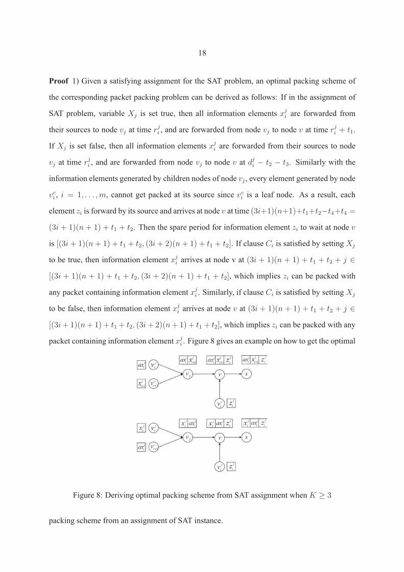
Proof 1) Given a satisfying assignment for the SAT problem, an optimal packing scheme of

the corresponding packet packing problem can be derived as follows: If in the assignment of

SAT problem, variable Xj is set true, then all information elements xji are forwarded from

their sources to node vj at time rji , and are forwarded from node vj to node v at time rji + t1.

If Xj is set false, then all information elements xji are forwarded from their sources to node

vj at time rji , and are forwarded from node vj to node v at dji − t2 − t3. Similarly with the

information elements generated by children nodes of node vj , every element generated by node

vci , i = 1, . . . , m, cannot get packed at its source since vci is a leaf node. As a result, each

element zi is forward by its source and arrives at node v at time (3i+1)(n+1)+t1+t2−t4+t4 =

(3i + 1)(n + 1) + t1 + t2. Then the spare period for information element zi to wait at node v

is [(3i+ 1)(n+ 1) + t1 + t2, (3i+ 2)(n+ 1) + t1 + t2]. If clause Ci is satisfied by setting Xj

to be true, then information element xji arrives at node v at (3i + 1)(n + 1) + t1 + t2 + j ∈

[(3i + 1)(n + 1) + t1 + t2, (3i + 2)(n + 1) + t1 + t2], which implies zi can be packed with

any packet containing information element xji . Similarly, if clause Ci is satisfied by setting Xj

to be false, then information element xji arrives at node v at (3i + 1)(n + 1) + t1 + t2 + j ∈

[(3i+ 1)(n+ 1) + t1 + t2, (3i+ 2)(n+ 1) + t1 + t2], which implies zi can be packed with any

packet containing information element xji . Figure 8 gives an example on how to get the optimal

Figure 8: Deriving optimal packing scheme from SAT assignment whenK ≥ 3

packing scheme from an assignment of SAT instance.

19

Under this scheme, no packet will contain more than 3 elements, which also satisfies the

packing size constraint. Every element zi, i = 1, . . . , m, can be packed at node v with a packet

containing message xji if clause Ci is satisfied due to variable Xj . Therefore, the additional

number of transmission to send each element zi to node s ism. As a result, the total number of

transmission for this tree is Ct0 +m = Ct1.

2) If we may find that the optimal packing scheme has a total number of transmission Ct1,

which implies that every element zi joins a packet consisting of xji for some j value. If x

ji leaves

from node vj at time rji + t1, and zi joins the packet that contains xji at node v, this can only

happen whenXj is unnegated in clauseCi because (3i+1)(n+1)+t1+t2+j ∈ [(3i+1)(n+1)+

t1+t2, (3i+2)(n+1)+t1+t2] and 3i(n+1)+j /∈ [(3i+1)(n+1)+t1+t2, (3i+2)(n+1)+t1+t2].

Thus we setXj to be true. If xji leaves from node v at time d

ji−(t2+ t3), and zi joins the packet

that contains xji at node v, this can only happen when Xj is negated in clause Ci because

(3i + 1)(n + 1) + t1 + t2 + j ∈ [(3i + 1)(n + 1) + t1 + t2, (3i + 2)(n + 1) + t1 + t2] and

(3i+2)(n+1)+ j+ t1+ t2 /∈ [(3i+1)(n+1)+ t1+ t2, (3i+2)(n+1)+ t1+ t2]. Thus we set

Xj to be false. By this way, if we have an optimal solution to this instance of packet packing

problem, we can have a satisfying assignment of the original SAT problem. Note that due to

Claim 3, the following case cannot happen: element zi gets packed with xji by letting x

ji leaves

node vj at time rji + t1, and in the meantime, that element zk gets packed with xjk by letting x

jk

leaves node vj at time djk − (t2 + t3).

Then, Claim 4 and the fact that the reduction shown in Figure 5 is a polynomial reduction

from SAT to P0 imply that P0 is strong NP-hard whenK ≥ 3.

Note that the above proof did not consider the impact of packet length on link reliability

and thus ETX. As long as we construct the reduction so that the ETX along links 〈vj, v〉, j =

1, . . . , n is significantly greater than that along link 〈v, s〉, however, the above analysis can beeasily extended to and still hold for cases where ETX is a function of packet length.

Having proved the strong NP-hardness of P0 when K ≥ 3, we analyze the hardness of

approximation for P0 using a gap-preserving reduction from MAX-3SAT to P0 [32], and we

have

20

Theorem 2 When K ≥ 3, there exists ε ≥ 1 such that it is NP-hard to achieve an approxima-

tion ratio of 1 + 1200N

(1 − 1ε) for problem P0, where N is the number of information elements

in P0.

Proof We first show that the reduction presented in Figure 5 is a gap-preserving reduction [32]

from MAX-3SAT to problem P0. It is easy to verify that the proof of Theorem 1 holds if the

discussion of the proof is based on 3SAT instead of the general SAT problem, in which case∑n

j=1 kj = 3m and we denote the reduction as f . Therefore, if a 3SAT problemΠ is satisfiable,

the minimum cost of the P0 problem Π′ = f(Π) is

Ct1 = Ct0 +m

= (∑n

j=1(2kj + 1) +∑n

j=1(kj + 1)(D + 1)+

2n(D + 1) + 2n+ 1) +m

= m(3D + 10) + n(3D + 6) + 1

(6)

Since n < 4m, (6) implies that

Ct1 < m(3D + 10) + n(3D + 10)

< 5m(3D + 10)

(7)

Note that the proof of Theorem 1 holds if D = n +∑n

j=1(2kj + 3) = 6m + n, which is the

number of information elements generated by the descendants of node v. Thus, (7) implies that

Ct1 < 5m(3(6m+ n) + 10)

= 5m(18m+ 3n+ 10)

< 5m(18m+ 3× 4m+ 10)

= 5m(30m+ 10)

< 5m(30m+ 10m)

= 200m2

(8)

21

If onlym0 of them clauses in Π are satisfiable, then the minimum cost in Π′ = f(Π) (with

K ≥ 3 is Ct1 +m−m0. This is because (m−m0) number of zi’s cannot be packed with any

other packet and have to be sent from node v to s alone, which incurs an extra cost of 1 each.

Accordingly, if less thanm0 of them clauses in Π are satisfiable, then the minimum cost C ′ in

Π′ = f(Π) is greater than Ct1 +m−m0. Letting ε = mm0, (8) implies that

C′

Ct1> Ct1+m−m0

Ct1

= Ct1+εm0−m0

Ct1

= 1 + (ε−1)m0

Ct1

> 1 + (ε−1)m0

200m2

= 1 + ε−1200m

1ε

= 1 + 1200m

(1− 1ε)

≥ 1 + 1200N

(1− 1ε)

(9)

where N is the number of non-sink nodes in the network and N ≥ m.

LetOPT (Π) andOPT (Π′) be the optima of a MAX-3SAT problemΠ and the correspond-

ing P0 problem Π′ = f(Π). Then the polynomial-time reduction f from MAX-3SAT to P0

satisfy the following properties:

OPT (Π) = 1 =⇒ OPT (Π′) = Ct1

OPT (Π) < 1ε

=⇒ OPT (Π′) > Ct1(1 +1

200N(1− 1

ε))

(10)

From [32], we know that there exists a polynomial-time reduction f1 from SAT to MAX-3SAT

such that, for some fixed ε > 1, reduction f1 satisfies

I ∈ SAT =⇒ MAX-3SAT(f1(I)) = 1

I /∈ SAT =⇒ MAX-3SAT(f1(I)) < 1ε

(11)

22

Then, (10) and (11) imply the following:

I ∈ SAT =⇒ OPT (f(f1(I))) = Ct1

I /∈ SAT =⇒ OPT (f(f1(I))) > Ct1(1 +1

200N(1− 1

ε))

(12)

Therefore, it is NP-hard to achieve an approximation ratio of 1 + 1200N

(1− 1ε) for problem P0.

Based on the definition of polynomial time approximation scheme (PTAS) and Theorem 2,

we then have

Corollary 1 There is no polynomial time approximation scheme (PTAS) for problem P0 when

K ≥ 3.

Based on the findings for P0, we have

Theorem 3 When K ≥ 3, problems P1, P2, and P are strong NP-hard whether or not the

routing structure is a tree or a linear chain, and there is no polynomial-time approximation

scheme (PTAS) for solving them.

Proof To prove the hardness results for P1, let’s consider a special case Π1 of P1 where 1)

every node is generating information elements using the same period p0 and the same spare

time s0 for information elements, 2) p0 is significantly larger than s0, and 3) p0 is significantly

larger than the latest time r0 when a node generates its first information element such that the

following holds: in the optimal packing scheme for Π1, no two elements from the same node

can be aggregated into the same packet, and the i-th information element from one node cannot

be packed with the j-th element from another node unless i = j. It is easy to see that the special

case Π1 does exist by properly choosing the parameters p0, s0, and r0. Therefore, solving Π1

becomes the same as solving an instance Π0 of P0 where the information elements consist of

the first element from every node of Π1. Therefore, P1 is at least as hard as P0. Since P0 is

strong NP-hard, P1 is strong NP-hard, and the there is no PTAS for the problem.

Since P1 is a special case of P2, and P2 is a special case of P, both P2 and P are strong

NP-hard too, and there is no PTAS for them.

23

Theorems 1 and 3 show that the joint optimization problems are strong NP-hard and there

is no PTAS, whether or not the routing structure is a tree or a linear chain and whether or

not the information elements are of equal length. In contrast, Becchetti et al. [10] showed

that, for total aggregation, the joint optimization problems are solvable in polynomial time via

dynamic programming on chain networks. Therefore, we see that aggregation constraints make

the difference on whether a problem is tractable for certain networks, and thus it is important

to consider them in the joint optimization. Incidentally, we note that Theorem 3 also answers

the open question on the complexity of Problem (P4) of batch-process scheduling in interval

graphs [22].

Complexity when K = 2

We showed in the previous section that the problems Pi, i = 0, 1, 2, and P are all strong NP-

hard and there is no PTAS for these problems whenK ≥ 3. We prove in this section that, when

K = 2, the complexity of these problems depends on whether information elements in a packet

can be separated and re-packed with other elements (which we call re-aggregation hereafter)

on their way to the sink. When re-aggregation is disallowed, these problems are solvable in

polynomial time; otherwise they are strong NP-hard. Note that, when K ≥ 3, these problems

are all strong NP-hard even if re-aggregation is disallowed, which can be seen from the proof of

Theorem 1. Note also that, even though re-aggregation may well be allowed in most sensornet

systems when the in-network processing (INP) method is packet packing, re-aggregation may

not be possible or allowed when INP is data fusion such as lossy data compression [67]. Via

the study on the impact of re-aggregation, therefore, we hope to shed light on the structure of

the joint optimization problems when general INP methods are considered.

In what follows, we first analyze the case when re-aggregation is allowed, then we analyze

the case when re-aggregation is disallowed.

When re-aggregation is allowed

Use a method similar to that of Theorem1, we prove the following theorem.

24

Theorem 4 When K = 2 and re-aggregation is allowed, problem P0 is strong NP-hard, and

this result holds whether or not the routing structure is a tree or a linear chain.

Proof Given an instance Π of SAT problem with n Boolean variables X1, . . . , Xn and m

clauses C1, . . . , Cm, we derive a polynomial time transformation from Π to an instance Π′′

of problem P0 with K = 2 as follows. The transformation is the same as what we present

through Figure 5 except for the following changes:

• Define a node p between node v and node s, andm children p1, . . . , pm of node p. Addi-tionally, define ETXvp = ETXps = ETXpip = 1, and tvp = t3, tps = t5, and tpip = t6.

• Define m information elements gi’s generated by nodes p1, , pm: gi : [rpi , dpi ] = [(3i +

1)(n+1)+n+0.1+ t1 + t2+ t3− t6, (3i+1)(n+1)+n+0.1+ t1 + t2+ t3+ t5], and

for node p, define an information element g with lifetime [5(m+ 1)2(n+ 1) + i, 5(m+

1)2(n+ 1) + i+ t5].

• For all parameters defined during the transformation in Figure 5, replace t3 by t3 + t5.

Therefore, the time complexity of the new transformation is still O(nm), and the new re-

duction is shown in Figure 9.

Then, the following claims hold for Π′′:

Claim 5 If nodes vc1, . . . , vcm, and nodes p1, . . . , pm are ignored, the minimum number of trans-

missions in Π′′ is C ′t0 =

∑n

j=1(2kj + 1) +∑n

j=1[(kj + 1)(D + 2)] + 2n(D + 2) + 2n+ 3.

Claim 6 If nodes vc1, . . . , vcm, and nodes p1, . . . , pm are ignored, in the optimal packing scheme

of Π′′, every information element q generated by a leaf node of node vj ,j = 1, . . . , n, is for-

warded to the source’s parent at time rq, and then leaves the parent to next hop either at time

rq + t1, or at time dq − (t2 + t3 + t5).

Claim 7 If nodes vc1, . . . , vcm, and nodes p1, . . . , pm are ignored, in the optimal packing scheme

of Π′′, for each j = 1, . . . , n, all the information elements xji leave node vj for v either at time

rji + t1, or at time dji − (t2 + t3 + t5).

25

Figure 9: Reduction from SAT to P0 when K = 2

These claims can be proved in the same way as how Claims 1, 2, and 3 are proved respec-

tively, and we skip the details here. Then, we propose

Claim 8 The minimal number of transmissions required in Π′′, denoted by C ′t1, is C ′

t0 + 4m if

and only if the SAT problem Π is satisfiable.

Proof 1) Given a satisfying assignment for the SAT problem, an optimal packing scheme of

the corresponding packet packing problem can be derived as follows: If in the assignment of

SAT problem, variableXj is set true, then all information elements xji are forwarded from their

sources to node vj at time rji , and are forwarded from node vj to node v at time rji + t1. If

Xj is set false, then all information elements xji are forwarded from their sources to node vj

at time rji , and are forwarded from node vj to node v at dji − (t2 + t3 + t5). Similarly with

the information elements generated by children nodes of node vj , every information element

generated by node vci , i = 1, . . . , m, cannot get packed at its source since vci is a leaf node.

As a result, each information element zi is forward by its source and arrives at node v at time

(3i + 1)(n + 1) + t1 + t2 − t4 + t4 = (3i + 1)(n + 1) + t1 + t2. Then the spare period for

information element zi to wait at node v is [(3i+1)(n+1)+ t1+ t2, (3i+2)(n+1)+ t1+ t2].

If clause Ci is satisfied by setting Xj to be true, then information element xji arrives at node v

26

at (3i+ 1)(n+ 1) + t1 + t2 + j ∈ [(3i+ 1)(n+ 1) + t1 + t2, (3i+ 2)(n+ 1) + t1 + t2], which

implies that zi can be packed with the packet containing information element xji . Similarly, if

clause Ci is satisfied by setting Xj to be false, then information element xji arrives at node v at

(3i+ 1)(n+ 1) + t1 + t2 + j ∈ [(3i+ 1)(n+ 1) + t1 + t2, (3i+ 2)(n + 1) + t1 + t2], which

implies zi can be packed with the packet containing information element xji . However, due

to the packet size constraint, one packet cannot contain more than 2 information elements. In

the meantime, every information element generated by node pi cannot get packed at its source

since node pi is a leaf node. Thus each information element gi is forwarded by its source and

arrives at node p at time (3i + 1)(n + 1) + n + 0.1 + t1 + t2 + t3. Then the spare period for

element gi to wait at node p is 0. In this case, to minimize the total number of transmission,

if clause Ci is satisfied by setting Xj to be true, information element xji arrives at node v with

information element axji−1 at time (3i+1)(n+1)+ t1+ t2+ j in one packet. When this packet

arrives at v, information element axji−1 and information element zi form a new packet while

information element xji waits at v until (3i+ 1)(n+ 1) + t1 + t2 + n+ 0.1. xj

i arrives at node

g at time (3i + 1)(n + 1) + n + 0.1 + t1 + t2 + t3 and forms a new packet with information

element gi. In this scheme, axji−1 first packed x

ji at node vj , then leaves x

ji at node v so that

xji can pack another information element gi some time later at node p, which implies that a

carry-over operation is used to achieve the optimal packing scheme. Similarly, if clause Ci is

satisfied by setting Xj to be false, element xji is arrives at node v with element ax

ji at time

(3i+1)(n+1)+ t1 + t2 + j in one packet. When this packet arrives at v, information element

xji and information element zi form a new packet while information element ax

ji waits at v until

(3i+1)(n+1)+t1+t2+n+0.1. axji arrives at node p at time (3i+1)(n+1)+n+0.1+t1+t2+t3

and forms a new packet with information element gi. In this scheme, xji first packed ax

ji at node

vj , then leaves axji at node v so that ax

ji can pack another information element gi some time

later at node p, which implies that a carry-over operation is used to achieve the optimal packing

scheme. An demonstration on how the optimal packing scheme is derived is given in Figure

10.

In the optimal packing scheme, every information element zi can be packed at node v with

27

Figure 10: Deriving optimal packing scheme from SAT assignment when K = 2

an information element xji or ax

ji−1 if clause Ci is satisfied due to variable Xj . Therefore, the

additional number of transmission to send each information element zi to node s ism, and the

additional number of transmission to send each information element gi to node s ism, and the

additional number of transmission to break up m packet at node v and send them to node s is

2m. As a result, the total number of transmission for this tree is C ′t0 + 4m = C ′

t1.

2) If we may find that the optimal packing scheme has a total number of transmission C ′t1,

which implies that every information element zi pack with one information element in a packet

consisting of xji for some j value, and the other information element in the old packet packs

with information element gi. If xji leaves from node vj at time r

ji + t1, and zi packs with one

information element in the packet that contains xji at node v, this can only happen when Xj is

unnegated in clauseCi because (3i+1)(n+1)+t1+t2+j ∈ [(3i+1)(n+1)+t1+t2, (3i+2)(n+

1)+t1+t2] and 3i(n+1)+j /∈ [(3i+1)(n+1)+t1+t2, (3i+2)(n+1)+t1+t2]. Thus we setXj

to be true. If xji leaves from node v at time d

ji−(t2+t3+t5), and zi packs with one information

element in the packet that contains xji at node v, this can only happen when Xj is negated in

clauseCi because (3i+1)(n+1)+t1+t2+j ∈ [(3i+1)(n+1)+t1+t2, (3i+2)(n+1)+t1+t2]

and (3i+2)(n+1)+ j + t1 + t2 /∈ [(3i+1)(n+1)+ t1 + t2, (3i+2)(n+1)+ t1 + t2]. Thus

we set Xj to be false. By this way, if we have an optimal solution to this instance of packet

28

packing problem, we can have a satisfying assignment of the original SAT problem. Note that

due to Claim 7, the following case cannot happen: element zi gets packed with xji by letting

xji leaves node vj at time r

ji + t1, and in the meantime, that element zk gets packed with xj

k by

letting xjk leaves node vj at time d

jk − (t2 + t3 + t5).

Then, Claim 8 and the fact that the reduction shown in Figure 9 is polynomial imply that

P0 is strong NP-hard whenK = 2.

Note that the above proof did not consider the impact of packet length on link reliability

and thus ETX. As long as we construct the reduction so that the ETX along links 〈vj, v〉, j =

1, . . . , n is significantly greater than that along links 〈v, p〉 and 〈p, s〉, however, the above anal-ysis can be easily extended to and still hold for cases where ETX is a function of packet length.

Note also that the above proof can be extended to the case when all the information elements

are generated at the same time, as well as the case when the routing structure is a linear chain

(with information elements having different generation time).

Then, we prove the hardness of approximation using a gap-preserving reduction from

MAX-3SAT, and we have

Theorem 5 When K = 2 and re-aggregation is allowed, there exists ε ≥ 1 such that it is

NP-hard to achieve an approximation ratio of 1 + 1120N

(1− 1ε) for problem P0, where N is the

number of information elements in P0.

Proof The proof is similar to that of Theorem 2.

We first show that the reduction presented in Figure 9 is a gap-preserving reduction [32]

from MAX-3SAT to problem P′0. It is easy to verify that the proof of Theorem 4 holds if

the discussion of the proof is based 3SAT instead of the general SAT problem, in which case∑n

j=1 kj = 3m and we denote the reduction as f . Therefore, if a 3SAT problemΠ is satisfiable,

29

the minimum cost of the P′0 problem Π′ = f(Π) is

C ′t1 = C ′

t0 + 4m

= (∑n

j=1(2kj + 1) +∑n

j=1(kj + 1)(D + 2)+

2n(D + 2) + 2n+ 3) + 4m

= m(3D + 16) + n(3D + 9) + 3

(13)

Since n < 4m, Equation 13 implies that

C ′t1 < m(3D + 16) + n(3D + 16)

< 5m(3D + 16)

(14)

Note that the proof of Theorem 4 holds if D = n +∑n

j=1(2kj + 3) = 6m + n, which is the

number of information elements generated by the descendants of node v. Thus, Equation 14

implies that

C ′t1 < 5m(3(6m+ n) + 16)

= 5m(18m+ 3n+ 16)

< 5m(18m+ 3× 4m+ 16)

= 5m(30m+ 16)

< 5m(30m+ 16m)

= 240m2

(15)

If onlym0 of them clauses in Π are satisfiable, then the minimum cost in Π′ = f(Π) (with

K = 3 is C ′t1+(m−m0). This is because (m−m0) number of zi’s cannot be packed with any

other packet and have to be sent from node v to s alone, which incurs an extra cost of 2 each.

Accordingly, if less thanm0 of them clauses in Π are satisfiable, then the minimum cost C ′ in

30

Π′ = f(Π) is greater than C ′t1 + 2(m−m0). Letting ε = m

m0, Equation 15 implies that

C′

C′t1>

C′t1+2(m−m0)

C′t1

=C′t1+2(εm0−m0)

C′t1

= 1 + 2 (ε−1)m0

C′t1

> 1 + 2 (ε−1)m0

240m2

= 1 + ε−1120m

1ε

= 1 + 1120m

(1− 1ε)

≥ 1 + 1120N

(1− 1ε)

(16)

where N is the number of non-sink nodes in the network and N ≥ m.

LetOPT (Π) andOPT (Π′) be the optima of a MAX-3SAT problemΠ and the correspond-

ing P′0 problem Π′ = f(Π). Then the polynomial-time reduction f from MAX-3SAT to P

′0

satisfy the following properties:

OPT (Π) = 1 =⇒ OPT (Π′) = C ′t1

OPT (Π) < 1ε

=⇒ OPT (Π′) > C ′t1(1 +

1120N

(1− 1ε))

(17)

From [32], we know that there exists a polynomial-time reduction f1 from SAT to MAX-3SAT

such that, for some fixed ε > 1, reduction f1 satisfies

I ∈ SAT =⇒ MAX-3SAT(f1(I)) = 1

I /∈ SAT =⇒ MAX-3SAT(f1(I)) < 1ε

(18)

Then, Equation 17 and 18 imply the following:

I ∈ SAT =⇒ OPT (f(f1(I))) = C ′t1

I /∈ SAT =⇒ OPT (f(f1(I))) > C ′t1(1 +

1120N

(1− 1ε))

(19)

Therefore, it is NP-hard to achieve an approximation ratio of 1 + 1120N

(1− 1ε) for problem P0.

31

We relegate the details to the appendix.

Based on the definition of polynomial time approximation scheme (PTAS) and Theorem 5,

we then have

Corollary 2 There is no polynomial time approximation scheme (PTAS) for problem P0 when

K = 2 and re-aggregation is allowed.

Based on the relations among P0, P1, P2, and P, we have

Theorem 6 When K = 2 and re-aggregation is allowed, problems P1, P2, and P are strong

NP-hard whether or not the routing structure is a tree or a linear chain, and there is no

polynomial-time approximation scheme (PTAS) for solving them.

Proof The proof is similar to that of Theorem 3.

Theorems 4 and 6 show that, whenK = 2 and re-aggregation is allowed, the joint optimiza-

tion problems are strong NP-hard whether or not the routing structure is a tree or a linear chain,

and whether or not the information elements are of the same length. That is, the complexity

of these problems when K = 2 and re-aggregation is allowed is very much similar to the case

when K ≥ 3.

When re-aggregation is prohibited

WhenK = 2 and re-aggregation is prohibited, we can solve problem P (and thus its special

versions P0, P1, and P2) in polynomial time by transforming it into a maximum weighted

matching problem in an interval graph. An interval graph GI is a graph defined on a set I of

intervals on the real line such that 1) GI has one and only one vertex for each interval in the

set, and 2) there is an edge between two vertices if the corresponding intervals intersect with

each other. Given an instance of problem P, we solve it using Algorithm 1 as follows:

For Algorithm 1, we have

Theorem 7 When K = 2 and re-aggregation is prohibited, Algorithm 1 solves problem P in

O(n3) time, where n is the number of information elements considered in the problem.This

32

Algorithm 1 Algorithm for solving P whenK = 2 and re-aggregation is prohibited1: Generate an interval graph GI(VI , EI) for problem P as follows:

• Select an arbitrary information element q generated by node vq at time rq and withspare time sq, define an interval [rq, rq + sq] for q on the real line.

• For each remaining information element p generated by node vp at time rp and withspare time sp, let node vpq be the common ancestor of vp and vq that is the farthestaway from R among all common ancestors of vp and vq, then define an interval[rq − tvqvpq + tvpvpq , rq − tvqvpq + tvpvpq + sq] for information element p.

• Let VI = ∅. Then, for each information element s, define a vertex s and add it to VI .

• Let EI = ∅. If the two intervals that represent any two information elements u andh overlap with each other, define an edge (u, h) and add it to EI ; then assign edge(u, h)with a weight com(u, h) = ETXvuhR(lu)+ETXvuhR(lh)−ETXvuhR(lu+lh),where lu and lh are the length of u and h respectively.

2: Solve the maximum weighted matching problem for GI using Edmonds’ Algorithm [24].3: For each edge (u, h) in the matching, information elements u and h are packed together atnode vuv. For all other vertices not in the matching, their corresponding information ele-ments are sent to the sink alone without being packed with any other information element.

holds whether or not the routing structure is a tree or a linear chain, and whether or not the

information elements are of equal length.

Proof It is easy to see that if information elements u and h are packed together, the total num-

ber of transmissions taken to deliver u and h is ETXvuR(lu) +ETXvhR(lh)−ETXvuhR(lu)−ETXvuhR(lh) +ETXvuhR(lu + lh) = ETXvuR(lu) +ETXvhR(lh)− com(u, h). Let VI be the

set of vertices in the interval graph GI , M be a matching in GI , V1 be the set of nodes in M ,

and V2 = VI/V1. Then the weight ofM , denoted byWM , is expressed in Equation 20:

Note that∑

v∈VIETXvR(lv) is a fixed value, and

∑(u,h)∈M [ETXvuR(lu)+ETXvhR(lh)−

com(u, h)] +∑

v∈V2ETXvR(lv) is the total number of transmissions, denoted by ETXtotal,

incurred in the packing scheme generated by Algorithm 1. Therefore, ETXtotal is minimized

if and only if WM is maximized, which means that solving the maximum weighted matching

problem can give us an optimal solution to the original packet packing problem.

33

WM =∑

(u,h)∈M com(u, h)

=∑

(u,h)∈M [ETXvuR(lu) + ETXvhR(lh)

−(ETXvuR(lu) + ETXvhR(lh)

−com(u, h))]

=∑

(u,h)∈M(ETXvuR(lu) + ETXvhR(lh))

−∑(u,h)∈M [ETXvuR(lu) + ETXvhR(lh)

−com(u, h)]

=∑

s∈V1ETXsR(ls) +

∑v∈V2

ETXvR(lv)

−{∑(u,h)∈M [ETXvuR(lu) + ETXvhR(lh)

−com(u, h)]

+∑

v∈V2ETXvR(lv)}

=∑

v∈VIETXvR(lv)

−{∑(u,h)∈M [ETXvuR(lu) + ETXvhR(lh)

−com(u, h)] +∑

v∈V2ETXvR(lv)}

(20)

Let n denote the total number of information elements in this problem. The whole algorithm

consists of three parts. The first one is to define an interval graph and assign weights to each

node and edge in the graph, whose time complexity is O(n2). The second part is to solve

the maximum weighted matching problem, whose time complexity is O(n3) by Edmonds’

Algorithm [24]. And the third part is to convert the optimal matching problem to the optimal

packing scheme, whose time complexity is O(n). Therefore, the time complexity of the whole

algorithm is O(n2) +O(n3) +O(n) = O(n3).

By the definition of the weight com(u, h) for elements u and h in Algorithm , the solution

generated by the maximum weighted matching tends to greedily pack elements as soon as pos-

sible after they are generated. This observation motivates us to design a local, greedy online

algorithm tPack in the next section for the general joint optimization problems, and the effec-

34

tiveness of this approach will be demonstrated through competitive analysis and testbed-based

measurement study in next two sections. Note that, incidentally, Theorem 7 also answers the

open question on the complexity of scheduling batch-processes with release times in interval

graphs [22].

A Utility-based online algorithm

We see from the complexity study section that problem P and its special cases in sensornets

are strong NP-hard in most system settings, and there is no polynomial-time approximation

scheme (PTAS) for these problems. Instead of trying to find global optimal solution, therefore,

we focus on designing a distributed, approximation algorithm tPack that optimizes the local

utility of packet packing at each node. Given that packet arrival processes are usually unknown

a priori, we consider the online version of the optimization problem.

Based on the definition of P, its optimization objective is to minimize

AC =TXnet∑x∈X lx

(21)

where TXnet is the total number of transmissions taken to deliver each information element

x ∈ X to the sink before its deadline. For convenience, we call AC the amortized cost of

delivering∑

x∈X lx amount of data. In what follows, we design an online algorithm tPack

based on this concept of amortized cost of data transmission. Accordingly, a local optimization

objective at a node j is to minimize

ACj =TXj

dataj(22)

where TXj is the total number of transmissions taken to deliver dataj amount of data from j

to the sink R before their deadline. Then an online algorithm, which we denote as tPack, is to

minimize ACj for the timely delivery of the data that node j currently holds.

When node j has a packet pkt in its data buffer, j can decide to transmit pkt immediately

35

or to hold it. If j transmits pkt immediately, information elements carried in pkt may be

packed with packets at j’s ancestors to reduce the amortized cost of data transmissions from

those nodes; if j holds pkt, more information elements may be packed with pkt so that the

amortized cost of transmission from j can be reduced. Therefore, we can define the utility of

transmitting or holding pkt as the expected reduction in amortized data transmission cost as a

result of the corresponding action, and then the decision on whether to transmit or to hold pkt

depends on the utilities of the two actions. For simplicity and for low control overhead, we only

consider the immediate parent of node j when computing the utility of transmitting pkt. We

will show the goodness of this local approach through competitive analysis later in this section

and through testbed-based measurement in next section.

In what follows, we first derive the utilities of holding and transmitting a packet, then we

present a scheduling rule that improves the overall utility.

Utility calculation

For convenience, we define the following notations:

L : maximum payload length per packet;

ETXjp(l) : expected number of transmissions taken to transport a

packet of length l from node j to its ancestor p;

pj : the parent of node vj in the routing tree.

The utilities of holding and transmitting a packet pkt at a node vj depend on the following

parameters related to traffic pattern:

• With respect to vj itself and its children:

rl : expected rate in receiving another packet pkt′ from a child or locally from an

upper layer;

sl : expected payload size of pkt′.

• With respect to the parent of vj :

36

rp : expected rate for the parent to transmit another packet pkt′′ that does not contain

information elements generated or forwarded by vj itself;

sp : expected payload size of pkt′′.

The utilities of holding and transmitting a packet pkt also depend on the following con-

straints posed by timeliness requirement for data delivery as well as limited packet size:

• Grace period t′f for delivering pkt: the maximum allowable latency in delivering pkt

minus the maximum time taken to transport pkt from vj to the sink without being held at

any intermediate node along the route.

If t′f ≤ 0, pkt should be transmitted immediately to minimize the extra delivery latency.

• Spare packet space s′f of pkt: the maximum allowable payload length per packet minusthe current payload length of pkt.

Parameter s′f and the size of the packets coming next from an upper layer at vj or from

vj’s children determine how much pkt will be packed and thus the potential utility of

locally holding pkt.

In the design and analysis of this section, we assume that packet arrival process (i.e.,, rl, rp),

packet payload size and spare space (i.e., sl, sp, s′f ), and grace period (i.e., t′f ) are independent

of one another. Then, the utilities of holding and transmitting a packet are calculated as follows.

Utility of holding a packet. When a node vj holds a packet pkt, pkt can be packed with

incoming packets from vj’s children or from an upper layer at vj . Therefore, the utility of hold-

ing pkt at vj is the expected reduction in the amortized cost of transmitting pkt after packing

pkt. The utility depends on (a) the expected number of packets that vj will receive within t′f

time (either from a child or locally from an upper layer), and (b) the expected payload size sl of

these packets. Given that the expected packet arrival rate is rl, the expected number of packets

to be received at vj within t′f time is t′frl. Thus, the expected overall size S ′l of the payload to

be received within t′f time is

S ′l =

t′ftlsl

37

Given the spare space s′f in the packet pkt, the expected size Sl of the payload that can bepacked into pkt can be approximated2 as

Sl = min{S ′l , s

′f} = min{t

′f

tlsl, s

′f}

Therefore, the expected amortized cost ACl of transporting the packet to the sink R after

the anticipated packing can be approximated as2

ACl =1

L− s′f + SlETXjR(L− s′f + Sl)

where (L− s′f ) is the payload length of pkt before packing.

Since the amortized cost AC ′l of transporting pkt without the anticipated packing is

AC ′l =

1

L− s′fETXjR(L− s′f)

the utility Ul of holding pkt is

Ul = AC ′l − ACl (23)

Utility of immediately transmitting a packet. If node vj transmits the packet pkt imme-

diately to its parent pj , the utility comes from the expected reduction in the amortized cost of

packet transmissions at pj as a result of receiving the payload carried by pkt. When vj transmits

pkt to pj , the grace period of pkt at pj is still t′f , thus the expected number of packets that do

not contain information elements from vj and can be packed with pkt at pj is t′frp, and we use

Ppkt to denote this set of packets. Given the limited payload that pkt carries, it may happen that

not every packet in Ppkt gets packed (to full) via the payload from pkt. Accordingly, the utility

Up of immediately transmitting pkt is calculated as follows:

• If every packet in Ppkt gets packed to full with payload from pkt, i.e., t′frp(L − sp) ≤L− s′f :

2We use this approximation because it is usually difficult to estimate and store the complete distributions ofrandom variables in resource-constrained sensor nodes.

38

Then, the overall utility U ′p can be approximated as 2

U ′p =

t′ftp

ETXpjR(sp)

t′ftp

sp

−t′ftp

ETXpjR(L)

t′ftp

L

=ETXpjR

(sp)

sp− ETXpjR

(L)

L

(24)

• If not every packet in Ppkt gets packed to full with payload from pkt, i.e., t′frp(L− sp) >

L− s′f :

In this case, �L−s′f

L−sp number of packets are packed to full; if mod(L − s′f , L − sp) > 0,

there is also a packet that gets partially packed with mod(L−s′f , L−sp) length of payloadfrom pkt. Thus the total number of packets that benefit from the packet transmission is

�L−s′f

L−sp�. Denoting mod(L − s′f , L − sp) by lmod and letting Imod be 1 if lmod > 0 and 0

otherwise, then the overall utility U ′′p can be approximated as2

U ′′p =

�L−s′

fL−sp

�ETXpjR(sp)

�L−s′

fL−sp

�sp

−

�L−s′

fL−sp

�ETXpjR(L)+ImodETXpjR

(sp+lmod)

�L−s′

fL−sp

�sp+L−s′f

(25)

Therefore, the utility Up of immediately transmitting pkt to pj can be computed as

Up =

⎧⎪⎨⎪⎩

U ′p if t′frp(L− sp) ≤ L− s′f

U ′′p otherwise

(26)

where U ′p and U ′′

p are defined in Equations (24) and (25) respectively.

39

Scheduling rule

Given a packet to be scheduled for transmission, if the probability that the packet is imme-

diately transmitted is Pt (0 ≤ Pt ≤ 1), then the expected utility Ut(Pt) is

Ut(Pt) = Pt × Up + (1− Pt)Ul

= Ul + Pt(Up − Ul)

(27)

where Up and Ul are the utilities of immediately transmitting and locally holding the packet

respectively. To maximize Ut, Pt should be set according to the following rule:

Pt =

⎧⎪⎨⎪⎩

1 if Up > Ul

0 otherwise

That is, the packet should be immediately transmitted if the utility of immediate transmission is

greater than that of locally holding the packet. For convenience, we call this local, distributed

decision rule tPack (for time-sensitive packing). Interested readers can find the discussion on

how to implement tPack in TinyOS in [68].

Competitive analysis

To understand the performance of tPack as compared with an optimal online algorithm, we

analyze the competitive ratio of tPack. Since it is difficult to analyze the competitive ratio of

non-oblivious online algorithms for arbitrary network and traffic pattern in the joint optimiza-

tion and tPack is a non-oblivious algorithm, we only study the competitive ratio of tPack for

complete binary trees where all the leaf nodes generate information elements according to a

common data generation process, and we do not consider the impact of packet length on link

ETX. We denote these special cases of problem P as problem P′. The theoretical analysis here

is to get an intuitive understanding of the performance of tPack; we experimentally analyze

the behaviors of tPack with different networks, traffic patterns, and application requirements

through testbed-based measurement in the performance evaluation section. We relegate the

40

study on the competitive ratio of tPack as well as the lower bound on the competitive ratio of

non-oblivious online algorithms for the general problem P as a part of our future work. (Note

that the best results so far on the lower bound of the competitive ratio of joint INP- and latency-

optimization also only considered the cases where only leaf nodes generate information ele-

ments [59], and these results are for oblivious algorithms and for cases where no aggregation

constraint is considered [59].)

Theorem 8 For problem P′, tPack ismin{K,maxvj∈V>1

2ETXvjR

2ETXvjR−ETXpjR

}-competitive, whereK is the maximum number of information elements that can be packed into a single packet, V>1

is the set of nodes that are at least two hops away from the sink R.

Proof For convenience, we denote the optimal packing scheme as OPT . By definition, tPack

is at least K-competitive since, considering the packets transmitted by a given node vi in the

routing tree, the length of the packet containing an information element x in OPT is no more

thanK times the length of the packet containing x in tPack.

To get a tighter performance bound for tPack, we first analyze the packet length for the

packets transmitted by a leaf node vj . Suppose that vj transmits a packet pkt with length lpkt

when the latency requirement could have allowed packing another l′ amount of data with the

packet. In this case, the utility of holding pkt is

Ul =ETXvjR

lpkt− ETXvjR

lpkt + l′= ETXvjR

l′

lpkt(lpkt + l′)(28)

By definition, the utility of immediately transmitting pkt is no more than the transmission

utility that would be generated if the information elements of pkt are all packed into another

packet pkt∗ at pj , the parent of vj , that was transmitted to pj from its the child other than vj .

Given that the routing tree is a complete binary tree and that the leaf nodes generate informa-

tion elements according to a common data generation process, the lengths of packets that are

transmitted along links at the same tree level are expected to be the same. Thus we can assume

that the payload length of pkt∗ is also lpkt. Therefore, the utility of immediately forwarding pkt

41

at vj satisfy the following inequality

Up ≤ETXpjR

lpkt− ETXpjR

lpkt + lpkt=

ETXpjR

2lpkt(29)

By the design of tPack, we know that Ul < Up. From (28) and (29), thus we have

ETXvjR

l′

lpkt(lpkt + l′)<

ETXpjR

2lpkt

Thus

l′ <a

2− alpkt (30)

where a =ETXpjR

ETXvjR.

Due to the constraint imposed by application’s requirement on the timeliness of data de-

livery, we know that the length of the packet, denoted by lopt, that contains the information

elements of pkt in OPT is no more than lpkt + l′. Then from (30), we know that

lopt ≤ lpkt + l′ <2

2− alpkt =

2ETXvjR

2ETXvjR −ETXpjR

lpkt

That is,loptlpkt

<2ETXvjR

2ETXvjR − ETXpjR

(31)

For a node vi that is not a leaf node, the same analysis applies. Given a packet pkt′ of length

lpkt′ that is transmitted by vi when the latency requirement could have allowed packing another

l′′ amount of data with pkt′, we have

l′′ <a′

2− a′lpkt′ (32)

where a′ = ETXpiR

ETXviR. Moreover, the length of the packet, denoted by lopt′ , that contains the

information elements of pkt′ in OPT is no more than lpkt′ + l′′; this is due to the following

reasons:

42

• If a packet pktmax contains lpkt′ + l′′ amount of data payload without constrained by

packet size limit, then the spare time of pktmax is 0.

• Consider a packet pkt′′ transmitted by vi in OPT whose length is lopt′ . If vi holds pkt′′

until its spare time is 0 (instead of transmitting pkt′′) in OPT, the resulting length of the

new packet pkt′′0 is no more than lpkt′ + l′′. This is because data flows faster toward the

sink in tPack as compared with OPT, and pkt′ reaches vi earlier than pkt′′ does.

• Therefore, lopt′ is no more than the length of pkt′′0 , which is no more than lpkt′ + l′′. Thus,

lopt′ ≤ lpkt′ + l′′

Therefore, we havelopt′

lpkt′<

2ETXviR

2ETXviR − ETXpiR

(33)

From (31) and (33), we know that tPack is at leastO(maxvj∈V>1

2ETXvjR

2ETXvjR−ETXpjR

)-competitive.

Therefore, tPack is min{K,maxvj∈V>1

2ETXvjR

2ETXvjR−ETXpjR

}-competitive for problem P′.

From Theorem 8, we see that tPack is 2-competitive if every link in the network is of equal

ETX value.

Implementation

From the discussion in last section, a node vj needs to obtain the following parameters when

calculating the utilities of holding and transmitting a packet:

• On routing tree: ETXjR(l), pj , and ETXpjR(l);

• On traffic pattern: rl, sl, rp, sp, andK.

Parameters related to routing tree can be provided by the routing component in a given

system platform. Given a link 〈j, p〉,ETXjp(l) as a function of packet length l can be estimated

using ETXjp(1), the ETX value of transmitting a packet of one unit length, as follows:

ETXjp(l) = 1/(1

ETXjp(1))l = ETXjp(1)

l

43

Accordingly, the routing component only needs to estimate ETXjp(1) instead of the ETX

values for packets of arbitrary length.

For parameters related to traffic pattern, vj can estimate by itself the parameters rl and sl,

andK is readily available and fixed for each specific platform. To enable each node vj to obtain

parameters rp and sp, every node i in the network estimates the expected rate ri to transmit two

consecutive packets at i itself and the expected size si of these packets. Then, every node i

shares with its neighbors the parameters ri and si by piggybacking these information onto data

packets or other control packets in the network. When a node vj overhears parameter rpj and

spj from its parent pj , vj can approximate rp and sp with rpj − rjsjspjand spj respectively. The

derivation is as follows.

Approximation of rp and sp: Since information elements generated or forwarded by the chil-

dren of node pj are treated in the same manner (without considering where they are from), the

expected size of the packet being transmitted by pj does not depend on whether the packet

contains information elements generated or forwarded by vj . Thus, vj can simply regard spj as

sp, the expected size of the packet transmitted by pj that does not contain information elements

coming from vj .

Now we derive rp as follows. Since the amount of payload transmitted by pj per unit time is

rpjspj and the amount of payload transmitted by vj is rjsj per unit time, the amount of payload

lp that are transmitted by pj but are not from vj per unit time is calculated as: lp = rpjspj−rjsj .

Thus, the expected rate rp that pj transmits packets that do not contain information elements

from vj is calculated as: rp = lp/spj = rpj − rjsjspj. Therefore, the expected interval tp between

pj transmitting two consecutive packets that do not contain information elements from vj is as

follows: tp = 1rp

=tpj×tj×spj

tj×spj−tpj×sj.

Performance evaluation

To characterize the impact of packet packing and its joint optimization with data delivery

timeliness, we experimentally evaluate the performance of tPack in this section. We first present

the experimentation methodology and then the measurement results.

44

Methodology

Testbed. We use the NetEye wireless sensor network testbed at Wayne State University

[3]. NetEye is deployed in an indoor office as shown in Figure 11. We use a 10 × 13 grid

Figure 11: NetEye wireless sensor network testbed

of TelosB motes in NetEye, where every two closest neighboring motes are separated by 2

feet. Out of the 130 motes in NetEye, we randomly select 120 motes (with each mote being

selected with equal probability) to form a random network for our experimentation. Each of

these TelosB motes is equipped with a 3dB signal attenuator and a 2.45GHz monopole antenna.

In our measurement study, we set the radio transmission power to be -25dBm (i.e., power

level 3 in TinyOS) such that multihop networks can be created. We also use channel 26 of the

CC2420 radio to avoid external interference from sources such as the campus WLANs. We

use the TinyOS collection-tree-protocol (CTP) [27] as the routing protocol to form the routing

structure, and we use the Iowa’s Timesync protocol [2] for network wide time synchronization.

Protocols studied. To understand the impact of packet packing and its joint optimization

with data delivery timeliness, we comparatively study the following protocols:3

• noPack: information elements are delivered without being packed in the network.

• simplePack: information elements are packed if they happen to be buffered in the samequeue, but there is not packing-oriented scheduling.

• SL: the spread latency algorithm proposed in [10], where the spare time of an informa-tion element is evenly spent at each hop from its source to the sink without considering

3We use the terms protocols, algorithms, and decision rules interchangeably in this paper.

45

specific network conditions (e.g., network-wide traffic pattern). SL was proposed with

total aggregation in mind without considering aggregation constraints such as maximum

packet size.

• CC: the common clock algorithm proposed in [10], where the spare time of an informa-tion element is only partly spent at the node where it is generated. Same as SL, CC was

proposed with total aggregation in mind.

• tPack: the packing- and timeliness-oriented scheduling algorithm that maximizes thelocal utility at each node, as we proposed in this chapter. (We have also evaluated another

version of tPack, denoted by tPack-2hop, where the forwarding utility Up considers both

the parent node and the parent’s parent; we find that tPack-2hop does not bring significant

improvement over tPack while introducing higher overhead and complexity, thus our

discussion here only focuses on tPack.)

We have implemented, in TinyOS [5], a system library which includes all the above proto-

cols. The implementation takes 40 bytes of RAM (plus the memory required for regular packet

buffers) and 4,814 bytes of ROM.

Performance metrics. For each protocol we study, we evaluate their behavior based on the

following metrics:

• Packing ratio: number of information elements carried in a packet;

• Delivery reliability: percentage of information elements correctly received by the sink;

• Delivery cost: number of transmissions required for delivering an information elementfrom its source to the sink;

• Deadline catching ratio: out of all the information elements received by the sink, thepercentage of them that are received before their deadlines;

• Latency jitter: variability of the time taken to deliver information elements from the samesource node, measured by the coefficient-of-variation (COV) [36] of information delivery

46

latency.

Traffic pattern. To experiment with different sensornet scenarios, we use both periodic data

collection traffic and event detection traffic trace as follows:

• D3: each source node periodically generates 50 information elements with an inter-

element interval, denoted by Δr, uniformly distributed between 500ms and 3s; this is to

represent high traffic load scenarios.

• D6: same as D3 except that Δr is uniformly distributed between 500ms and 6s; this is

to represent relatively low traffic load scenarios.

• D9: same asD3 except that Δr is uniformly distributed between 500ms and 9s.

• Elites: an event traffic where a source node generates one packet based on the Lites [1]

sensornet event traffic trace.

To understand the impact of the timeliness requirement of data delivery, we experiment with

different latency requirements. For periodic traffic, we consider maximum allowable latency in

delivering information elements that is 1, 3, and 5 times the average element generation period,

and we denote them by L1, L3, and L5 respectively; for event traffic, we consider maximum

allowable latency that is 2s, 4s, or 6s, and we denote them by L2′, L4′, and L6′ respectively. Out

of the 120 motes selected for experimentation, we let the mote closest to a corner of NetEye

be the sink node, and the other mote serves as a traffic source if its node ID is even. For

convenience, we regard a specific combination of source traffic model and latency requirement

a traffic pattern. Thus we have 8 traffic patterns in total. To gain statistical insight, we repeat

each traffic pattern 20 times. Note that, in each traffic pattern, all the information elements

have the same maximum allowable latency. In our implementation, each information element

is 16-byte long, and the TelosB motes allow for aggregating up to 7 information elements into

a single packet (i.e., K = 7).

47

Figure 12: Packing ratio: D3

Measurement Results

In what follows, we first present the measurement results for periodic traffic patterns D3,

D6, and D9, then we discuss the case of event traffic pattern Elites. In most figures of this sec-

tion, we present the means/medians and their 95% confidence intervals for the corresponding

metrics such as the packing ratio, delivery reliability, delivery cost, deadline catching ratio, and

the latency jitter.4

Periodic Data Traffic

For the periodic traffic pattern D3, Figures 12-16 show the packing ratio, delivery relia-

bility, delivery cost, deadline catching ratio, and latency jitter in different protocols. tPack

tends to enable higher degree of packet packing (i.e., larger packing ratio) than other protocols

except the CC protocol. The increased packing in tPack reduces channel contention and thus

reduces the probability of packet transmission collision, which improves data delivery reliabil-4The distributions for delivery reliability and latency jitter are not symmetric, thus we use medians instead of

means to summarize their properties [36].

48

Figure 13: Delivery reliability: D3

Figure 14: Delivery cost: D3

49

Figure 15: Deadline catching ratio: D3

Figure 16: Latency jitter: D3

50

Figure 17: Histogram of routing hop count: D3 with maximum latency L1

ity. The reduced probability of transmission collision and the increased number of information

elements carried per packet in tPack in turn reduces delivery cost, since there are fewer num-

ber of packet retransmissions as well as fewer number of packets generated. Note that the low

delivery reliability in simplePack is due to intense channel contention.

Exceptions to the above general observation happen in the case of maximum allowable

latency L1 or when comparing tPack with CC. In the first case, the packing ratio in tPack is

lower than that in SL, but tPack still achieves much higher delivery reliability (i.e., by more

than 40%) and much lower delivery cost (i.e., by a factor of more than 3). This is because the

packing ratio in SL is too high such that, in the presence of high wireless channel contention

due to the high traffic load of D3 and the stringent real-time requirement of L1, the resulting

long packet length leads to higher packet error rate and lower packet delivery reliability (as

shown in Figure 13). The routing protocol CTP adapts to the higher packet error rate in SL,

and this leads to longer routes and larger routing hops in SL. This can be seen from Figure 17

which shows the histogram of routing hop counts in different protocols. The maximum hop

51

count in tPack is 4, whereas the hop count can be up to 9 in SL. Together, the higher packet

error rate and the longer routes in SL lead to larger delivery cost in SL as compared with tPack.

Similar arguments apply to the case when comparing tPack with CC. From these data on the

benefits of tPack in comparison with SL and CC, we can see the importance of adapting to

network conditions and data aggregation constraints in in-network processing. Note that similar

arguments also explain the phenomenon where SL has higher packing ratio than simplePack

but lower delivery reliability and higher delivery cost under all latency settings of D3 traffic.

Figure 13 also shows that tPack improves data delivery reliability even when the allowable

latency in data delivery is small (e..g, in the case of L1) where the inherent probability for

packets to be packed tends to be small. Therefore, tPack can be used for real-time applications

where high data delivery reliability is desirable. Figure 12 shows that the packing ratio in tPack

is close to 4 except for the case of L1 where 1) too much packing is undesirable as discussed

earlier and 2) the packing probability is significantly reduced by the limited probability for

a node to wait due to stringent timeliness requirement. Our offline analysis shows that the

optimal packing ratio is ∼5 for the traffic patterns D3-L3 and D3-L5; thus tPack achieves a

packing ratio very close to the optimal, which corroborates our analytical result in Theorem 8.

Figure 15 shows the deadline catching ratio in deadline-aware data aggregation schemes

tPack, SL, and CC. Though the deadline catching ratio of all the three protocols are close to

1, the catching ratio of tPack is the highest and is greater than 0.99 in all cases. The slightly

higher deadline catching ratio in tPack is a result of its online adaptation of packet holding

time at each hop according to in-situ channel and traffic conditions along the path. As a re-

sult of the properly controlled packet packing, the reduced channel contention and improved

packet delivery reliability in tPack also help enable lower performance variability. For instance,

Figure 16 shows the latency jitter in different protocols, and we see that the jitter tends to be

the lowest in tPack, especially when the real-time requirement is stringent (e.g., in L1 and

L3). These properties are desirable in cyber-physical-system (CPS) sensornets where real-time

sensing and control require predictable data delivery performance (e.g., in terms of low latency

jitter), especially in the presence of potentially unpredictable, transient perturbations.

52



53



54



55



56



57

Figures 18-22 and Figures 23-27 show the measurement results for periodic traffic patterns

D6 and D9 respectively. We see that, in terms of relative protocol performance, the overall

trends in D6 and D9 are similar to those in D3. For instance, with stringent real-time require-

ment in L1, SL achieves a lower delivery reliability and a higher delivery cost than tPack even

though the packing ratio tends to be higher in SL. Due to the reduced traffic load and thus the

reduced wireless channel contention and collision, however, the delivery reliability of noPack,

simplePack, and SL is also relatively high compared with their delivery reliability in D3.

Note that, in [10], CC is shown to have a much higher competitive ratio than SL through

theoretical analysis. From our measurement study, however, we see that the performance of

CC is not always better than SL. For instance, CC has a lower delivery reliability and a higher

delivery cost than SL in D6 − L5. This seemingly discrepancy is due to the fact that the

theoretical analysis of [10] does not consider the limit of data aggregation capacity, nor does it

consider wireless link unreliability and interference in scheduling.

Surprisingly, Figures 18-20 show that, for the traffic pattern D6, simplePack introduces

higher delivery cost than noPack does even though the packing ratio and the end-to-end de-

livery reliability are higher in simplePack. One reason for this is that, partially due to the

increased packet length in simplePack, the link reliability in simplePack is lower than that in

noPack as shown in Figure 28.5 The routing protocol CTP adapts to the lower link reliability in

simplePack and introduces longer routing hop length, which can be seen from Figure 29 which

shows the histogram of routing hop counts for noPack and simplePack in traffic patternD6-L1.

Together, the lower link reliability and the longer routes in simplePack introduce larger infor-

mation delivery cost when compared with noPack inD6. This observation is also corroborated

by the detailed analysis of the cost (e.g., mean number of transmissions) taken to deliver an

information element. For instance, Figure 30 shows the mean cost of delivering an information

element from a node at different geographic distances (in terms of the number of grid hops)

from the base station for the traffic pattern D6-L1. (Similar phenomena are observed for other5The reason why simplePack still has higher end-to-end information element delivery reliability despite its

lower link reliability is because each packet delivered in simplePack carries more information elements due to thehigher packing ratio.

58

Figure 28: Link reliability: D6

Figure 29: Histogram of routing hop count: D6 with maximum latency L1

59

Figure 30: Per-element delivery cost vs. geo-distance: D6 with maximum latency L1

traffic patterns.) We see that, for most of the cases, the per-element delivery cost is higher in

simplePack. Note that similar arguments explain why simplePack has higher delivery cost

than noPack in traffic pattern D9 and why SL also has higher delivery cost than noPack in sev-

eral cases (e.g., for traffic pattern D6-L1). In view with the consistently better performance in

tPack, these observations demonstrate again the importance of considering network conditions

and data aggregation constraints in in-network processing.

Event Traffic

Figures 31-35 show the measurement results for event traffic pattern Elites. The overall

trend on the relative protocol performance is similar to that in the periodic traffic patterns D3,

D6, and D9. Even though the delivery reliability tends to be high for all protocols, tPack still

achieves lower delivery cost and latency jitter, as well as 100% deadline catching ratio.

Related work

In-network processing (INP) has been well studied in sensornets, and many INP methods

have been proposed for query processing [54, 69, 55, 58, 15, 14, 49, 30] and general data

60

Figure 31: Packing ratio: Elites

Figure 32: Delivery reliability: Elites

61

Figure 33: Delivery cost: Elites

Figure 34: Deadline catching ratio: Elites

62

Figure 35: Latency jitter: Elites

collection [20, 21, 43, 52, 61, 71]. When controlling spatial and temporal data flow to enhance

INP, however, these methods did not consider application requirements on the timeliness of

data delivery. As a first step toward understanding the interaction between INP and applica-

tion QoS requirements, our study has shown the benefits as well as the challenges of jointly

optimizing INP and QoS from the perspective of packet packing. As sensornets are increas-

ingly being deployed for mission-critical tasks, it becomes important to address the impact of

QoS requirements on general INP methods other than packet packing, which opens interesting

avenues for further research.

As a special INP method, packet packing has also been studied for sensornets as well as

general wireless and wired networks, where mechanisms have been proposed to adjust the de-

gree of packet packing according to network congestion level [29, 35], to address MAC/link

issues related to packet packing [48, 53, 46], to enable IP level packet packing [40], and to

pack periodic data frames in automotive applications [62]. These works have focused on is-

sues in local, one-hop networks without considering requirements on maximum end-to-end

63

packet delivery latency in multi-hop networks. With the exception of [62], these works did not

focus on scheduling packet transmissions to improve the degree of packet packing, and they

have not studied the impact of finite packet size either. Saket et al. [62] studied packet pack-

ing in single-hop controller-area-networks (CAN) with finite packet size. Our work addresses

the open questions on the complexity and protocol design issues for jointly optimizing packet

packing and data delivery timeliness in multi-hop wireless sensornets.

Most closely related to our work are [10] where the authors studied the issue of optimiz-

ing INP under the constraint of end-to-end data delivery latency. But these studies did not

consider aggregation constraints and instead assumed total aggregation where any arbitrary

number of information elements can be aggregated into one single packet. These studies did

not evaluate the impact of joint optimization on data delivery performance either. Our work

focuses on settings where packet size is finite, and we show that aggregation constraints (in

particular, maximum packet size and re-aggregation tolerance) significantly affect the problem

complexity and protocol design. Using a high-fidelity sensornet testbed, we also systemati-

cally examine the impact of joint optimization on packet delivery performance in multi-hop

wireless networks. By showing that tPack performs better than the algorithm SL and CC [10],

our testbed based measurement results also demonstrate the benefits of considering realistic

aggregation constraints in the joint optimization.

Solis et al. [63] also considered the impact that the timing of packet transmission has on data

aggregation, and the problem of minimizing the sum of data transmission cost and delay cost

has been considered in [59] and [38]. These studies also assumed total aggregation, and they

did not consider hard real-time requirements on maximum end-to-end data delivery latency.

Ye et al. [70] considered the local optimal stopping rule for data sampling and transmission in

distributed data aggregation. It did not consider hard real-time requirement either, and it did not

study network-wide coordination and the limit of data aggregation. Yu et al. [72] studied the

latency-energy tradeoff in sensornet data gathering by adapting radio transmission rate; it did

not study the issue of scheduling data transmission to improve the degree of data aggregation.

64

Concluding remarks

Through both theoretical and experimental analysis, we examine the complexity and impact

of jointly optimizing packet packing and the timeliness of data delivery. We find that aggre-

gation constraints (in particular, maximum packet size and re-aggregation tolerance) affect the

problem complexity more than network and traffic properties do, which suggest the importance

of considering aggregation constraints in the joint optimization. We identify conditions for the

joint optimization to be strong NP-hard and conditions for it to be solvable in polynomial time.

For cases when it is polynomial-time solvable, we solve the problem by transforming it to the

maximum weighted matching problem in interval graphs; for cases when it is strong NP-hard,

we prove that there is no polynomial-time approximation scheme (PTAS) for the problem. We

also develop a local, distributed online protocol tPack for maximizing the local utility of each

node, and we prove the competitiveness of the protocol with respect to optimal solutions. Our

testbed-based measurement study also corroborates the importance of QoS- and aggregation-

constraint aware optimization of packet packing.

While this chapter has extensively studied the complexity, algorithm design, and impact

of jointly optimizing packet packing and data delivery timeliness, there are still a rich set of

open problems. Even though we have analyzed the competitiveness of tPack for non-trivial

scenarios and this has given us insight into the behavior of tPack, it remains an open question

on how to characterize in a closed form the competitiveness of tPack and non-oblivious online

algorithms in broader contexts. The analytical and algorithmic design mechanisms developed

for packet packing may well be extensible to address other in-network processing methods such

as data fusion, and a detailed study of this will help us better understand the structure of the

joint optimization problem and will be interesting future work to pursue. We have focused on

the scheduling aspect of the joint optimization, and we are able to use mathematical tools such

as interval graphs to model the problem; on the other hand, how to mathematically model and

analyze the impact of the joint optimization on spatial data flow is still an open question and

is beyond the scope of most existing network flow theory, thus it will be interesting to explore

65

new approaches to modeling and solving the joint optimization problem.

66

CHAPTER 3

ENERGY-EFFICIENT NETWORK CODING BASED ROUTING

Preliminary

Ahlswede et al. [6] first proposed the network coding technique. The authors showed that

the use of network coding can effectively increase throughput in wired networks. Since then,

different network coding strategies have been studied, e.g., linear network coding [6], non-

linear network coding [45] and random network coding [31] [34]. Ho et al. [31] proved that

the use of random network coding can achieve the theoretical maximal throughput in wireless

networks. And Eryilmaz et al. [18] show that network coding can reduce transmission latency,

therefore can increase the throughput in multicast traffic flow.

Recently, Chachulski et al. [13] propose MORE, the first protocol to integrate random net-

work coding with opportunistic routing for unicast flow in wireless mesh networks. Experiment

results show that MORE yields a higher network throughput than ExOR [12] which only uses

opportunistic routing. Based on the framework of [13], [50] [41] further improve the network

throughput by introducing different ACK and rate control schemes. To the best of our knowl-

edge, however, there has been no systemic study on spatial and energy consumption control on

network-coding-based (NC-based) routing, which is of great importance in power-constrained

distributed systems, e.g., wireless sensor networks.

In this work, we study the open problem of minimal cost NC-based routing in wireless

networks. Our main contributions are as follows.

• We propose an effective load based approach to measure the expected number of trans-missions of NC-based transmission for arbitrary topologies. This is the first mathematical

framework to compute the transmission cost of NC-based routing.

• We propose a polynomial greedy algorithm to compute the minimal transmission costand the corresponding routing braid for NC-based routing. We prove the optimality of

67

this algorithm and an upper bound of transmission cost for the optimal NC-based routing

braid, which is equal to the cost of shortest single path routing.

• Based on the algorithm we proposed, we design and implement EENCR, an energy-efficient NC-based routing protocol, for resource-constrained sensor platforms. In EENCR,

we incorporate the 4-bit link estimator of CTP [27], realize a light-weight distributed im-

plementation for our greedy forwarder set selection algorithm in the rouging engine,

and design a modified null-spaced-based (M-NSB) coded feedback scheme and a corre-

sponding rate control component. Compared to CTP, EENCR introduces zero additional

communication cost but yields an optimal routing braid with lower cost than the shortest

single path routing.

• We evaluate the performance of EENCR on the NetEye testbed by comparing it with CTP[27], MORE [13] and CodeOR [50]. Experiment results show that EENCR achieves a

close to 100% reliability with a large transmission cost reduction of CTP, i.e., 25 - 28%.

And EENCR further improves the goodput of NC-based routing protocol by adaptively

selecting the forwarders instead of utilizing the whole forwarder candidate set.

The remaining of this chapter is organized as follows. We first introduce the system settings

and problem definition. We then propose the effective-load-based framework to compute the

transmission cost of NC-based routing. Based on this framework, we design a polynomial-time

greedy algorithm that can compute the optimal routing braid for arbitrary topologies. Next we

present EENCR, which includes a distributed implementation of our greedy algorithm. We

evaluate the performance of EENCR under different topologies on the NetEye testbed. Before

we conclude this chapter, we discuss related work in the field of network coding.

System settings and problem definition

In this section, we first present the system settings we used in this study. Next we explain

why we choose intra-flow network coding in designing efficient routing protocol for mission-

68

critical WCPS. Based on the system model, we formally define the problems of transmission

cost computation and optimization for NC-based routing.

System settings

In this study, we model a wireless network as a graphG = (V,E)with node S as the source

and T as the destination. For each node i ∈ G, we useUi andDi to denote the set of senders and

receivers of i, respectively. And we denote the forwarder set of i as FSi ⊂ Di. For each link

i→ j ∈ E, we denote ETXxij as its expected number of transmission to deliver a packet with

length x and P xij =

1ETXij

as the corresponding link reliability. Since network coding will not

change the packet length during the transmission, we use ETXij and Pij for simplicity. Then

we define CiT (x) as the transmission cost of delivering x linear independent packets from i to

T , and CiDi(x) as the expected number of broadcasts of node i when nodes in Di collectively

receive x linear independent coded packets from i. Assuming S needs to deliverK packets as

a batch to T , we define Kji as the number of linear independent packets node i received from

node j.

Comparison between inter-flow and intra-flow network coding

In studies of network coding in wireless environment, there are two general techniques. The

first one is inter-flow network coding, which allows a node to encode packets from different

flows and broadcast the coded packet. The second one is intra-flow network coding, which

allows a node only encode packets of the same flow and broadcast the coded packet. Both

techniques have their advantages and suitable application scenarios. Inter-flow network coding

suits well for multiple source-destination pairs in a wireless environment while intra-flow net-

work coding suits better for single unicast data flow in wireless networks. In mission-critical

WCPS, the most common traffic flow is called convergecast, in which multiple sources send

data to single destination. Convergecast is a variant of both multiple source-destination flows

and single unicast flow. Theoretically, we can use both inter-flow and intra-flow technique to

improve the energy efficiency of convergecast in WCPS. However, inter-flow coding requires

69

perfect feedback information for a sending node to make encoding decision. This requirement

incurs very high communication overhead and therefore makes inter-flow network coding un-

favorable for convergecast applications in WCPS. Furthermore, applying inter-flow coding in

convergecast also requires defining auxiliary nodes in the network, which will make the whole

solution too complex for mission-critical WCPS. On the contrary, intra-flow coding requires

little feedback information. Not only will this feature of intra-flow coding makes it suitable for

efficiency improvement inWCPS, but also it will make the protocol design and implementation

simpler for resource-constrained sensor platforms.

Problem definition

We define the minimal cost NC-based routing problem as follows:

Problem Q0 Given a graph G = (V,E) with one source S and one destination T , find the

optimal total transmission cost and the corresponding FSi for each node i to deliverK packets

using intra-flow random network coding from S to T .

To the best of our knowledge, however, there has been no study on how to measure the

transmission cost of intra-flow network coding, letting alone the optimal transmission cost.

Therefore, we need to first find a way to measure the transmission cost of NC-based routing

before we can solveQ0. Therefore, we define the following problem:

ProblemQ1 the same asQ0 except that FSi = Di for each node i.

The solution to problemQ1 can provide a mathematical framework to compute the expected

transmission cost of NC-based routing. Not only will this framework provide a tool for our

solution to problemQ0, but also it will shed lights towards energy-efficiency study of NC-based

transmission in future study. In the following sections, we will propose optimal polynomial-

time algorithms for both problemQ1 andQ0.

70

Cost optimization for NC-based routing

In this section, we first propose an effective load assignment algorithm to solve problemQ1.

The key idea of this algorithm is to compute the number of encoded packets each intermediate

node should forward and the corresponding cost. Based on this approach, we then design

a distributed polynomial-time algorithm to optimally solve Q0. For each node i in Q0, we

choose the forwarder set FSi out of Di using a greedy algorithm based on the transmission

cost from each node inDi to T We prove this algorithm’s optimality and show that the optimal

transmission cost of NC-based routing has an upper bound that equals to the transmission cost

of the shortest path routing.

Effective load based assignment algorithm forQ1

In NC-based opportunistic routing protocols, such as MORE [13], the network throughput

is significantly improved compared with single path routing. However, the transmission cost

of these protocols are not carefully controlled and it may be higher than the cost of single path

routing since every intermediate node will forwards re-encoded packets to its own forwarder

candidate set. To precisely measure and control the transmission cost while still fully utilizing

the benefit of network coding on throughput, we propose a concept called effective load.

Definition 1 For a node j in the forwarder candidate set FCSi, the effective load Lj is defined

as the number of linear independent packets that are received by j but not by any of the other

nodes in FCSi that has lower transmission cost to the destination.

To demonstrate this concept, we first look at the following example in Figure 36. In this

example, the source node S has K = 3 packets that needs delivering to T and CAT < CBT .

Therefore, node A has a higher priority than B in FCSS . When S stops broadcasting, the

coding vectors of packets received by node A are {1, 2, 3} and {1, 1, 1} and the vectors at nodeB are {2, 3, 5} and {1, 1, 1}. Since node A has a lower transmission cost to T than B, node Ahas an effective load LA = 2. Node B only has an effective load LB = 1 because the packet

with coding coefficient {1, 1, 1} is also received by A. If both node A and B forward up to

71

their effective load of re-encoded packets to T , T will receive 3 linear independent packets,

which is just enough to decode the whole batch. In the meantime, there will be no unnecessary

re-encoding forwarding operations from FSCS to T .

Figure 36: An illustrating example of NC-based routing

Based on the concept of effective load, we then propose a framework to compute the trans-

mission cost of NC-based routing based on different effective load between nodes within the

same forwarder candidate set, i.e., given a node i, each node j ∈ Di will forward Lj linear

independent packets to the destination

To better illustrate how to use the effective load approach to compute the transmission cost

of NC-based routing, we first study the following example in Figure 37.

In this diamond topology, we define that P2 ≥ P4 ≥ P6. The whole transmission process

can be divided into two steps. The first step is node S broadcasting toDS = {A,B,C} and thesecond step is nodes in DS forwarding re-encoded packets to T . In the first step, we treat node

A,B,C as one single virtual node VDS. The link reliability of link S → VDS

is then expressed

as PSVDS= 1− (1− P1)(1− P3)(1− P5). Therefore, the transmission cost for the first step is

72

Figure 37: Example topology

CSDS(K) =

K

PSVDS

=K

1− (1− P1)(1− P3)(1− P5)(34)

In the second step, since we have P2 ≥ P4 ≥ P6, we want path A → T to forward as

many packets as it is capable of and path C → T to forward as least packets as needed. To

compute the effective load for nodes inDS, we first computeKi, the expected number of linear

independent packets received by each node from S in the first step.

⎧⎪⎪⎪⎪⎪⎨⎪⎪⎪⎪⎪⎩

KSA =

KP1

1− (1− P1)(1− P3)(1− P5)

KSB =

KP3

1− (1− P1)(1− P3)(1− P5)

KSC =

KP5

1− (1− P1)(1− P3)(1− P5)

(35)

Using Li to denote the number of linear independent packets node i needs to forward to T ,

it is easy to see that LA = KSA. However, we cannot simply calculate LB asmin(K−LA, K

SB)

because node B and A may receive some same packets, resulting in less entropy held by B.

Instead, we need to compute KS′

B , the expected number of linear independent packets that are

received by node B but not A.

KS′

B = KKS

B

K(1− P1) = KS

B(1− P1) (36)

73

The detailed deduction to compute KS′

B is to solve an easy probability theory problem and

is hence omitted. It is easy to see thatKS′

B < K−LA, thus we have LB = KBS′. Similarly, we

have LC = KS′

C = KSC(1−P1)(1−P3) and we can verify that LA+LB+LC = K. Combining

these intermediate results, we have the total transmission cost computed as:

CS(K) = CSDS(K) + CAT (LA)

+CBT (LB) + CCT (LC)

=K

1− (1− P1)(1− P3)(1− P5)

+LA

P2

+LB

P4

+LC

P6

=K

1− (1− P1)(1− P3)(1− P5)

[1 +P1

P2+

P3(1− P1)

P4+

P5(1− P1)(1− P3)

P6]

(37)

Through this example, we demonstrate how to compute the transmission cost of NC-based

routing. The basic idea is to first compute the broadcast cost treating all the nodes in the

forwarder candidate set as one single virtual node, and then compute the effective load, i.e., the

number of re-encoded packets needs to be forwarded at each node in the forwarder candidate

set based on an non-decreasing order of their cost to the destination.

Although the topology in Figure 37 consists of only node-disjoint paths from the source to

the destination, we can generalize this approach to recursively compute the cost of NC-based

routing in arbitrary topologies. We formally present this computing process as Algorithm 2.

Basically, each node i runs Algorithm 2 to compute its transmission cost to the destination if

every node in Di has its transmission cost computed and updated. Node i then sends its own

cost information to its sender(s). The sender(s) then run this algorithm again to compute their

transmission cost to the destination. By the end of this backwards recursive process, the source

node S will be able to compute its transmission cost to the destination based on the transmission

cost of nodes in DS. Note that the complexity of Algorithm 2 is O(|V | lg |V |), which makes itsuitable for power-constrained computation platforms, e.g., the Telosb sensor platform.

74

Algorithm 2 Compute the transmission cost of NC-based routing for the current node S withM forwarder candidates1: Input: current node S,DS = {A1, A2, . . . , AM}2: Output: CS(1): the expected number of transmissions to deliver 1 packet from S to T3: Sort nodes inDS by a non-descending order of CAi

(1), where i = 1, 2, . . . ,M .4: Sorted nodes are labeled as {A′

1, A′2, . . . , A

′M}

5: CSDS(1) = 1

1−∏M

i=1(1−PSA′

i)

6: LA′1= CSDS

(1)PSA′1

7: F = 1− PSA′1

8: for i→ 2, 3, . . . ,M do9: LA′i

= CSDS(1)PSA′i

F10: CA′i

(LA′i) = LA′i

CA′i(1)

11: F = F (1− PSA′i)

12: end for13: CS(1) = CSDS

(1) +∑M

i=1CA′i(LA′i

)

As described above, the major principle we use here is to always assign more traffic load

to forwarders with lower cost, which implies that we should apply different utilization of for-

warders in the DAG to minimize the transmission cost instead of fully utilizing every possible

path in the network. This observation provides two insights: 1)it shows that we do not need

full network coding redundancy in the network to perform regular data transmission, which

would cause higher transmission cost and contention; 2) extra redundancy may be used to pro-

vide proactive protection to mission-critical networks against single node failures. These two

insights lead us to the solution to problemQ0 in this chapter and problemQ in Chapter 4.

Optimal NC-based transmission cost algorithm

In the last section, we proposed a distributed algorithm executed by each node to compute

the transmission cost of NC-based routing from a given source to the destination. However,

there still lacks a precise control on transmission cost in NC-based routing, making NC-based

transmission energy-inefficient. This energy-inefficiency is especially severe in dense networks

where each node has many forwarder candidates.

In MORE-based protocols, forwarder candidates with low expected effective load are usu-

ally not allowed to forward the flow to reduce the contention in the network, which can reduce

the transmission cost sometimes. However, this reduction is not guaranteed and sometimes it

75

may even increase the transmission cost. Based on the observations we had a priori, we design

a distributed greedy algorithm, Algorithm 3. The basic idea of Algorithm 3 is as follows. For

an input node S, we first sort all nodes in DS in a non-descending order of their transmission

cost to the destination. We then remove the node A′i with the lowest transmission cost from

the sorted DS, add it to the forwarder set FSS and compute the total transmission cost using

Algorithm 2. If the transmission cost of S can be reduced by adding A′i to FSS, we keep it in

FSS and add another node with the lowest cost from the remaining sorted DS . We continue

this loop until either of the following two conditions is satisfied:

1. the sortedDS is empty, i.e., all receivers of S have been selected into the FSS;

2. moving another node from the sorted DS to FSS would increase the total transmission

cost from S to T .

Each non-destination node executes this algorithm to determine the minimal transmission

cost from itself to the destination T and the corresponding forwarder candidate set. Upon the

convergence of the whole network, we will get the solution to problemQ0.

Algorithm 3 Compute the minimal transmission cost of NC-based routing and the correspond-ing FCS for the input node S withM forwarders1: Input: node S,DS = {A1, A2, . . . , AM}, FSS = ∅2: Output: C∗

S(1): the minimal transmission cost to deliver 1 packet from S to T3: Sort nodes inDS by a non-descending order of CAi

(1), where i = 1, 2, . . . ,M .4: Sorted nodes are labeled as {A′

1, A′2, . . . , A

′M}

5: FSS = {A′1}

6: C∗S(1) =

1PSA′

1

+ CA′1(1)

7: for i→ 2, 3, . . . ,M do8: Run Algorithm 2 with input S and DS = {A′

1, . . . , A′i}

9: Get the result as CnewS (1)

10: if CnewS (1) > CS(1) then

11: break12: else13: FSS = FSS ∪A′

i

14: C∗S(1) = Cnew

S (1)15: end if16: end for

76

The complexity of this algorithm is O(|V |2 lg |V |). In NC-based routing, the size of FCS

can also be one and in this case the routing braid is the equivalent to the shortest single path.

Next we show readers the optimality of this algorithm by proving the following theorem:

Theorem 9 Given a node S and its forwarder candidate set DS = {A1, A2, . . . , AM}, Algo-rithm 3 yields the minimal transmission cost to the destination node of NC-based routing and

the corresponding forwarder set.

Proof We prove the correctness of this theorem by contradiction. Given a node S and its

forwarder candidate set DS , we denote the minimal transmission cost as C∗ and the corre-

sponding transmission forwarder set is FS∗S with a cardinality of k. We sort nodes in FS∗

S in

non-descending order of their transmission cost to the destination and denote them as FS∗S =

{A∗1, A

∗2, . . . , A

∗k} where CA∗

1≤ CA∗

2≤, . . . ,≤ CA∗

k.

If this theorem is not correct, then there exists at least one node Ax having CAx≤ CA∗i

for

some integer i ∈ [1, k]. Without loss of generality, we assume that CA∗k−1≤ CAx

≤ CA∗k. We

will have a contradiction when we can find a forwarder set FS∗∗S that has a lower transmission

cost C∗∗ than C∗. To find this contradiction, we study the following forwarder sets:

FS∗S = {A∗

1, A∗2, . . . , A

∗k}

FS1S = FS∗

S − {A∗k}

FS2S = FS∗

S ∪ {Ax}

(38)

For each forwarder set, we compute the transmission cost for these forwarder sets using

Algorithm 2. The transmission cost of FS∗S is expressed as:

C∗ =1 +

∑k

i=1[CA∗iPSA∗i

∏i−1j=1(1− PSA∗j

)]

1−∏k

i=1(1− PSA∗i)

(39)

Compared with FS∗S , FS1

S does not have node A∗k, therefore cost C1 is expressed as:

C1 =1 +

∑k−1i=1 [CA∗i

PSA∗i

∏i−1j=1(1− PSA∗j

)]

1−∏k−1i=1 (1− PSA∗i

)(40)

77

On the other hand, FS2S consists of both FS∗

S and node Ax. Since Ax has a lower transmis-

sion cost than node A∗k, we compute C2 as:

C2 =1

1− (1− PSAx)∏k

i=1(1− PSA∗i)

·{1 +∑k−1i=1 [CA∗i

PSA∗i

∏i−1j=1(1− PSA∗j

)] + CAxPSAx

∏k−1i=1 (1− PSA∗i

)

+PSA∗k(1− PSAx

)∏k−1

i=1 (1− PSA∗i)}

(41)

Based on our assumption, C∗, C1 and C2 have the following relations:

C∗ − C1 ≤ 0

C∗ − C2 ≤ 0(42)

The basic idea next is to prove that C∗ − C2 ≥ 0 when C∗ − C1 ≤ 0, which leads to a

contradiction.

C∗

C1=

1−∏k−1i=1 (1− PSA∗i

)

1−∏k

i=1(1− PSA∗i)· 1 +

∑k

i=1[CA∗iPSA∗i

∏i−1j=1(1− PSA∗j

)]

1 +∑k−1

i=1 [CA∗iPSA∗i

∏i−1j=1(1− PSA∗j

)]≤ 1

⇔ [1−∏k−1i=1 (1− PSA∗i

)] · {1 +∑k

i=1[CA∗iPSA∗i

∏i−1j=1(1− PSA∗j

)]}

−[1−∏k

i=1(1− PSA∗i)] · {1 +∑k−1

i=1 [CA∗iPSA∗i

∏i−1j=1(1− PSA∗j

)]} ≤ 0

⇔ {1 +∑k−1i=1 [CA∗i

PSA∗i

∏i−1j=1(1− PSA∗j

)]} · {∏k

i=1(1− PSA∗i)−∏k−1

i=1 (1− PSA∗i)}

+[1−∏k−1i=1 (1− PSA∗i

)]PSA∗kCA∗

k

∏k−1i=1 (1− PSA∗i

) ≤ 0

⇔ {1 +∑k−1i=1 [CA∗i

PSA∗i

∏i−1j=1(1− PSA∗j

)]} · (−PSA∗k)

+[1−∏k−1i=1 (1− PSA∗i

)]PSA∗kCA∗

k≤ 0

⇔

1 +∑k−1

i=1 [CA∗iPSA∗i

∏i−1j=1(1− PSA∗j

)] ≥ [1−∏k−1i=1 (1− PSA∗i

)]CA∗k

(43)

To accomplish this goal, we conduct some mathematical transformation of two inequities

78

above. The first inequity is between C∗ and C1. Starting from the fact that C∗

C1≤ 1, we have a

useful result in Equation 43:

And the second result is betweenC∗ and C2 and this time we directly expand the difference:

C∗ − C2 =1 +

∑k

i=1[CA∗iPSA∗i

∏i−1j=1(1− PSA∗j

)]

1−∏k

i=1(1− PSA∗i)

− 1

1 − (1− PSAx)∏k

i=1(1− PSA∗i)

·{1 +∑k−1i=1 [CA∗i

PSA∗i

∏i−1j=1(1− PSA∗j

)] + CAxPSAx

∏k−1i=1 (1− PSA∗i

)

+CA∗kPSA∗

k(1− PSAx

)∏k−1

i=1 (1− PSA∗i)}

= {1 +∑k−1i=1 [CA∗i

PSA∗i

∏i−1j=1(1− PSA∗j

)]}

·{ 1

1−∏k

i=1(1− PSA∗i)− 1

1− (1− PSAx)∏k

i=1(1− PSA∗i)}

+∏k−1

i=1 (1− PSA∗i)

·{PSA∗kCA∗

k[

1

1−∏k

i=1(1− PSA∗i)− 1− PSAx

1− (1− PSAx)∏k

i=1(1− PSA∗i)]

−PSAxCAx

· 1

1− (1− PSAx)∏k

i=1(1− PSA∗i)}

(44)

Using some simple technique, we further transform the right-hand of Equation 44 and have

the following result in Equation 45:

Using the result of Inequality 43 and the fact that CA∗k> CAx

, we can find that the right

hand side of Equation 45 is greater than 0, which means C∗ > C2 and shows the existence

of a contradiction. And we note that using the above mathematical deduction framework, a

contradiction can be found for any number of is where i ∈ [1, k] and CA∗i> CAx

. Therefore,

we proved that we can find the minimal transmission cost of S to the destination by adding

forwarder candidates with lower transmission cost to the destination into the forwarder set until

adding more candidates will increase the CS. By now, we complete our proof on the optimality

of Algorithm 3 in computing the optimal NC-based routing topology.

79

C∗ − C2 = {1 +∑k−1i=1 [CA∗i

PSA∗i

∏i−1j=1(1− PSA∗j

)]}

· PSAx

∏k

i=1(1− PSA∗i)

[1−∏k

i=1(1− PSA∗i)][1− (1− PSAx

)∏k

i=1(1− PSA∗i)]

+PSAx

∏k−1i=1 (1− PSA∗

i)

1− (1− PSAx)∏k

i=1(1− PSA∗i)· [ PSA∗

kCA∗

k

1−∏k

i=1(1− PSA∗i)− CAx

]

=PSAx

∏k−1i=1 (1− PSA∗i

)

[1−∏k

i=1(1− PSA∗i)][1− (1− PSAx

)∏k

i=1(1− PSA∗i)]

·{{1 +∑k−1i=1 [CA∗

iPSA∗

i

∏i−1j=1(1− PSA∗

j)]}(1− PSA∗

k)

+PSA∗kCA∗

k− [1−∏k

i=1(1− PSA∗i)]CAx

}

=PSAx

∏k−1i=1 (1− PSA∗i

)

[1−∏k

i=1(1− PSA∗i)][1− (1− PSAx

)∏k

i=1(1− PSA∗i)]

·{{1 +∑k−1i=1 [CA∗i

PSA∗i

∏i−1j=1(1− PSA∗j

)]}(1− PSA∗k)

+PSA∗kCA∗

k− PSA∗

kCAx

− [1− PSA∗k−∏k


=PSAx

∏k−1i=1 (1− PSA∗i

)

[1−∏k

i=1(1− PSA∗i)][1− (1− PSAx

)∏k

i=1(1− PSA∗i)]

{(1− PSA∗k){1 +∑k−1

i=1 [CA∗iPSA∗i

∏i−1j=1(1− PSA∗j

)]

−[1 −∏k


}

+ · PSA∗kCA∗

k− PSA∗

kCAx

}

(45)

A theoretical comparison with other routing protocols

In the previous section, we proposed an optimal greedy algorithm that computes the min-

imal transmission cost of NC-based routing. Different from the heuristic control of spatial

diversity in other MORE-based network coding opportunistic routing protocols, this algorithm

intelligently explores the routing diversity in wireless transmission and only adds routes that can

reduce the transmission cost into the forwarding topology. Therefore, our algorithm has a lower

transmission cost than existing NC-based protocols [13] [41] [50]. When implementing a rout-

ing protocol, nonetheless, we still need to face the choice between NC-based routing and single

path routing. In this section, we study a few properties of our solution, which demonstrates the

80

advantage of our NC-based transmission algorithm over traditional single path routing in terms

of energy efficiency, i.e., transmission cost.

In traditional single path routing, it is the common sense that we always want to select the

shortest path in the network. The term ”shortest” depends on different metrics or constraints we

use, e.g., transmission cost, hop count, capacity and latency. However, when we use intra-flow

network coding to tackle the forwarder selection problem in opportunistic routing to minimize

the transmission cost, the first property we find for our solution is that the shortest (i.e., lowest

cost) single path is not necessarily chosen into the transmission topology. This property is

formally presented in the following theorem:

Theorem 10 Given a node S with a candidate set FCSS of M forwarders, the optimal for-

warder set FSS computed in Algorithm 3 does not always contain node A∗ where A∗ ∈ FCSS

and 1PSA∗

+ CA∗ ≤ 1PSAi

+ CAifor any i ∈ FCSS/{A∗}.

Proof The proof of this theorem is not complex. As long as we give an instance of node S

with M forwarders that has the minimal cost transmission topology not including the lowest

cost single path, we have the proof we need. Thus we build an instance in Figure 38.

In this instance, the lowest cost single path is S → A3 → T with a cost 10.9

+ 10.1

= 11.11.

After we run Algorithm 3, however, the optimal forwarder set we have is FSS = {A1, A2}because we have the following results:

C{A1,A2} = 11−(1−0.1)(1−0.15)

· [1 + 0.10.4

+ 0.15(1−0.1)0.2

]

= 10.235

· (1 + 14+ 0.135

0.2)

= 8.1915

C{A1,A2,A3} = 11−(1−0.1)(1−0.15)(1−0.9)

· [1 + 0.10.4

+ 0.15(1−0.1)0.2

+ 0.9(1−0.1)(1−0.15)0.1

]

= 10.9235

· (1 + 14+ 0.135

0.2+ 0.6885

0.1)

= 9.5398 > C{A1,A2}

(46)

Using this instance, we finish our proof for this theorem.

81

Figure 38: Routing braid v.s. single path routing

From this example, it is also easy to see that the optimal transmission cost of NC-based

transmission is lower than that of shortest single path routing. This further raises the ques-

tion: will the minimal cost of NC-based transmission always be better than that of single path

routing? To answer this question, we propose the following theorem:

Theorem 11 Given a node S with a candidate set FCSS ofM forwarders, the optimal trans-

mission cost C∗S computed in Algorithm 3 is always lower than or equal to 1

PSA∗+CA∗where

A∗ ∈ FCSS and 1PSA∗

+ CA∗ ≤ 1PSAi

+ CAifor any i ∈ FCSS/{A∗}.

Proof Through Theorem 10 we showed that the forwarder on the lowest cost single path is not

always in the forwarder set computed in Algorithm 3. Therefore, we prove the correctness of

this theorem under two different cases:

1) A∗ /∈ FSS When the forwarder A∗ on the lowest cost single path is not selected into FSS ,

based on the greedy construction order of FSS , we have the following inequity:

82

CA∗ ≥ CAjfor any Aj ∈ FSS (47)

The only reason the algorithm does not add A∗ into FSS is because this operation will

increase the total NC-based transmission cost. We denote FSS = {A1, A2, . . . , Ak}. Thisargument can be mathematically expressed as:

C∗S − CFSS∪{A∗} =

1+∑k

i=1[CAi

PSAi

∏i−1

j=1(1−PSAj

)]

1−∏k

i=1(1−PSAi)

−1+∑k

i=1[CAi

PSAi

∏i−1

j=1(1−PSAj

)]+CA∗PSA∗∏k

i=1(1−PSA∗

i)

1−(1−PSA∗)∏k

i=1(1−PSAi

)

= {1 +∑k

i=1[CAiPSAi

∏i−1j=1(1− PSAj

)]}

·{ 1

1−∏k

i=1(1−PSAi

)− 1

1−(1−PSA∗)∏k

i=1(1−PSAi

)}

− CA∗PSA∗∏k

i=1(1−PSA∗

i)

1−(1−PSA∗)∏k

i=1(1−PSAi

)

={1+

∑ki=1[CAi

PSAi

∏i−1

j=1(1−PSAj

)]}PSA∗∏k

i=1(1−PSA∗i)

{1−∏k

i=1(1−PSAi

)}{1−(1−PSA∗ )∏k

i=1(1−PSAi

)}

−CA∗ ·PSA∗

∏ki=1(1−PSA∗

i)

1−(1−PSA∗)∏k

i=1(1−PSAi

)

=PSA∗

∏ki=1

(1−PSA∗i)

1−(1−PSA∗)∏k

i=1(1−PSAi)· {1+

∑ki=1

[CAiPSAi

∏i−1

j=1(1−PSAj

)]

1−∏k

i=1(1−PSAi)

− CA∗}

< 0

(48)

From this inequity, we then conduct the following transformation:

1+∑k

i=1[CAi

PSAi

∏i−1

j=1(1−PSAj

)]

1−∏k

i=1(1−PSAi)

− CA∗} < 0

⇔ C∗S − CA∗ < 0

⇒ C∗S < 1

PSA∗+ CA∗

(49)

Therefore, when A∗ is not selected into FSS, the optimal NC-based transmission cost C∗S

is lower than the transmission cost of shortest single path routing.

2) A∗ ∈ FSS In this case, we consider three scenarios:

a) If FSS = {A∗}, it is clear that C∗S = 1

PSA∗+ CA∗ .

83

b) If FSS �= {A∗} and A∗ is the first node selected into FSS, C∗ < 1PSA∗

+ CA∗ is implied in

the greedy forwarder selection process of Algorithm 3.

c) If FSS �= {A∗} and A∗ is not the first node selected into FSS, it is straightforward that

1

1− (1− PSA∗)∏i∈FSS

i (1− PSAi)>

1

PSA∗(50)

And it is implied in the greedy forwarder selection process that before adding A∗ into FSS ,

CA∗ is greater than or equal to the forwarding cost from the old FSS to the destination.

Therefore we still have C∗ < 1PSA∗

+ CA∗ under this scenario.

Combining all different scenarios, we can reach the conclusion that the minimal cost of

NC-based transmission is always smaller than or equal to the shortest single path routing. This

completes our proof.

Protocol design and implementation

After we proposed a minimal cost NC-based routing algorithm and proved its advantage

over traditional shortest single path routing through theoretical analysis, we move on to deploy

this algorithm into resource-constrained wireless platforms, e.g. wireless sensor networks. Not

only do we need to implement this core algorithm, we also need other components to build

the whole routing protocol. When designing a NC-based routing protocol, there are three key

challenges, which are:

1. For each node, which neighbor of it should be selected into the forwarder set?

2. For each node, howmany times of broadcast it should conduct for a batch before it stops?

3. For each node, how fast it should broadcast a re-encoded packet for a batch?

To address these challenges, we propose the energy-efficient NC-based routing (EENCR)

protocol to perform minimal cost NC-based transmission in wireless sensor networks. EENCR

84

is a fully distributed routing protocol that runs on every node in the network. In this section, we

present three key components of EENCR, each of which addresses one of the challenges listed

above.

Routing engine

Run on each node, the routing engine component computes the optimal forwarder set for

the current node, which address the first challenge. We design the routing engine in EENCR

based on the 4-bit link estimator component and routing engine component of the collection

tree protocol(CTP). Our routing engine is responsible for the following assignments:

(a) Estimate the single link reliability from the current node to each of its 1-hop neighbor;

(b) Compute and update the minimal cost of NC-based transmission from the current node

to the designated destination based on the received transmission cost information from its

neighbors;

(c) Broadcast the computed minimal cost and the forwarder set effective load table to all its

1-hop neighbor;

(d) Provide the optimal effective load information to the ACK component and the rate control

component.

The key difference between the routing engine in EENCR and CTP is that instead of select-

ing only the neighbor on the shortest single path as the next hop forwarder, EENCR selects a set

of neighbors into the forwarder set using Algorithm 3 such that the total transmission cost can

be further reduced. In this way, we make use of the routing diversity of wireless communication

to the max extent.

Modified NSB coded feedback

The routing engine component decides the forwarder set for the current node. In NC-based

routing, each node needs to knowwhen it can stop broadcasting to its forwarders. The condition

85

for a node i to stop broadcast is that nodes in the forwarder set of i have collectively receive

Li linear independent packets, where Li is the effective load information computed from the

routing engine component.

The usual way node i gets information to decide when to stop transmitting is via the ACK

feedback from nodes in FSi. One naive approach is to make nodes in FSi transmit ACK on a

per-packet basis. However, this per-packet ACK cannot be used in EENCR due to two reasons.

• The total size of per-packet ACK for the whole effective load is too large. In practicalnetwork coding protocols with symbol size GF (28) and batch size 8, each coding vector

contains 8 bytes. If a forwarder j wants to convey the whole coding vector space it

received from i, it will needKji 8-byte vectors, which is too large for energy-constrained

sensor networks.

• Sending back per-packet ACKs will introduce high-contention and communication over-head in the network, which reduces the energy-efficiency of the whole protocol.

One approach to avoid this high overhead is to use coded feedback. First proposed in

[60], the null-space-based (NSB) coded feedback scheme is originally designed to enhance

reliability of an NC-based multicast protocol for multimedia applications in mobile ad hoc

networks. To apply coded feedback into NC-based opportunistic routing, a Coded Cumulative

ACK (CCACK) was proposed in [41]. CCACK designs a more complex ACK generating and

testing scheme to solve the collective-space problem and false-positive problem when directly

applying NSB in NC-based opportunistic routing. However, CCACK is designed to deploy in

wireless mesh networks, where each node has a stronger computation power and larger storage

space. It is hard to transplant it into sensor networks because:

• Compared to NSB, CCACK needs a much larger storage space to storeM multiple hash

metrics, whereM ≥ 1;

• To decrease the probability of false-positive, CCACK needs to run test algorithms Mtimes, each of which with a different hash metrics;

86

Although CCACK can reduce the false-positive probability from 128to ( 1

28)M , it introduces

both higher memory overhead and computation overhead. And whenM = 1, the false-positive

probability of CCACK is the same as NSBwhile having a more complex computation overhead.

In fact, to overcome the collective-space problem in NC-based transmission, we only need a

modified NSB ACK scheme (M-NSB) instead of the more complex CCACK.

We first elaborate how the original NSB ACK works. We denote the set of coding vectors

received by node i to be Bri . When node i wants to broadcast about the feedback information

of linear independent packets it currently has, it generates the feedback information as a vector

zi that satisfies:

zi · v = 0, ∀v ∈ Bri (51)

Let V ri denote the linear space spanned by vectors in Br

i . It is shown in [60] that:

Lemma 1 With the above random construction of zi, any vector v′ ∈ V ri must satisfy zi ·v′ = 0.

And for any vector v′′ /∈ V ri , the probability of zi · v′′ = 0 is 1

28when GF (28) is used.

The reason why NSB coded feedback may cause the collective-space problem is because

NSB is not designed to convey the collective space of all downstream nodes but only the space

relationship between the individual node pairs. To overcome this shortcoming while keeping

the implementation at a low complexity level, we design the M-NSB coded feedback scheme.

M-NSB has two different features from the original NSB:

1. Instead of generating zi for set Bri , M-NSB generates zi for set Bw

i , which is the coding

vector set of all the re-encoded packets node i broadcasts. Then the condition zi needs to

satisfy becomes:

zi · v = 0, ∀v ∈ Bwi (52)

2. Node i stops broadcasting when there are Li vectors in Bwi are marked to be received by

nodes in FSi.

87

After a M-NSB ACK is generated, it is broadcast by the receiving node. M-NSB is dif-

ferent from CCACK in that M-NSB does not take nodes overhearing from different upstream

nodes into account. This is for the objective of precisely measuring and controlling the total

transmission cost for the whole network. In EENCR, each node has its own effective load and

packets received by the same node but from different senders will be viewed as different traffic

flows. By solving the collective-space problem for each sender separately, every coded packet

can be effectively used for the decoding at the destination. Therefore, M-NSB addresses the

second challenge in designing NC-based routing protocols.

Rate control

In EENCR, the routing engine component provides the effective load information, and the

M-NSB component provides the receipt status of re-encoded packets to the forwarder set. We

then design a rate control component to help each node decide when to start the broadcast and

how fast it should broadcast.

We first give the following definition of traffic flow:

Definition 2 A traffic flow f is defined as a 5-tuple f = (S, T, x, j, i) to represent a load of

packets originated at node S and destined at T with batch index x, which is forwarded from

sender j to forwarder i.

At each non-destination node i, EENCR maintains an array Bvi (f) to store linear indepen-

dent packets received for each flow. We also define a binary active-flow indicator If for each

flow (S, x, j, i). If is set to be false by default and is updated to true only when one of the

following two conditions is satisfied:

1. Node i is the first member of FSj for flow f ;

2. Node i receives more than Ki(f) − Li(f) linear independent packets from node j for

flow f , where Ki(f) is the number of linear independent packets i expected to receive

from j for flow and Li(f) is the effective load assignment of node i for flow f .

88

Every time there is a transmission opportunity for node i, one active-flow is chosen in

a round-robin fashion. A re-encoded packet is generated by selecting non-zero elements in

GF (28) as re-encoding vectors for packets in Bvi (f). Node i then broadcasts this re-encoded

packet and adding the re-encoding vectors intoBwi (f). Once the forwarder set of i has received

Li(f) linear independent packets, If is set to false and the array for flow f will be flushed.


To characterize the feasibility and effectiveness of network coding in improving the energy

efficiency , we experimentally evaluate the performance of EENCR in this section. We first

present the experimentation methodology and then the measurement results.

Methodology

Testbed. We use the NetEye wireless sensor network testbed at Wayne State University

[3]. Different from the environment of NetEye presented in Chapter 2, We have moved NetEye

to a new location since 2011 due to university arrangements. Nonetheless, we did our best to

keep the basic features of NetEye unchanged in the new location. In the new NetEye, we still

deployed 130 TelosB motes, where every two closest neighboring motes are separated by 2 feet

in an indoor environment. But the layout of the whole testbed is no longer a regular grid due to

the constraints of the room.

Out of the 130 motes in NetEye, we randomly select 40 motes (with each mote being



In our measurement study, we set the radio transmission power to be -7dBm (i.e., power

level 15 in TinyOS) such that multihop networks can be created. And we use the default MAC

protocol provided in TinyOS 2.x.

Protocols studied. To understand the impact of network coding in improving the energy

efficiency of wireless sensor networks, we comparatively study the following protocols:

89

• EENCR: the distributed NC-based routing protocol we proposed, which selects the opti-mal forwarder set for each node to minimize the transmission cost;

• CTP: a state-of-the-art collection tree protocol designed for data collection in sensornetworks [27];

• MORE: the first NC-based opportunistic routing protocol that fully explores the routingdiversity in the network by letting each forwarder to forward randomly coded packets;

• CodeOR: a NC-based opportunistic routing protocol that increases the concurrency ofdata flow by adding hop-by-hop ACK to the prototype of MORE.

We implement all four protocols in TinyOS 2.x. Due to the constraints of memory space of

TelosB motes, which is only 10 kilobytes, and the short data payload length in sensor network

applications, we choose a batch size of 8 for network coding operation instead of the mostly

used batch size of 32 in wireless mesh networks.

Performance metrics. For each protocol we study, we evaluate their behavior based on the

following metrics:



• Goodput: number of valid information elements received by the sink per second;

• Routing diversity: number of forwarders selected to transmit a packet.

Different from the throughput metric used to evaluate the performance of NC-based routing

protocols in [13] [50], in this study we use goodput instead. An information element is defined

as valid if and only if it is linear independent to all elements that are in the same batch and

90

received by the sink. And we do not study the routing diversity of CTP because its number of

forwarders to transmit a packet is always one.

Traffic pattern. To experiment with both light and heavy traffic scenarios, we use two

periodic data collection traffic patterns as follows:

• S10: out of all 40 nodes in the networks, 10 are selected as source nodes; Each source

node periodically generates 40 information elements with an inter-element interval, de-

noted by Δr, uniformly distributed between 500ms and 3s; for EENCR, MORE and

CodeOR, every consecutive 8 information elements compose a batch; this is to represent

light traffic load scenarios.

• S20: same as S10 except that 20 nodes are selected as source nodes; this is to represent

heavy traffic load scenarios.

Measurement results

In what follows, we first present the measurement results for light traffic pattern S10, then

we discuss the case of heavy traffic pattern S20. In the figures of this section, we present the

means and their 95% confidence intervals for the corresponding metrics.

Light data traffic

For the light traffic pattern S10, Figures 39 - 41 show the delivery reliability, delivery cost

and goodput of different protocols. We found that EENCR and CTP provide high data delivery

reliabilities (both are close to 100%) while MORE and CodeOR can only delivery 78% and

85% of the data to the sink on average. In the meantime, EENCR has a much lower delivery

cost than CTP, i.e. a 26% reduction, in terms of average number of transmissions to deliver

a packet but the delivery costs of MORE and CodeOR are around 400% and 300% of CTP

respectively. Furthermore, EENCR enables a higher data goodput very close to the theoretical

maximal value than all other three protocols.

The reasons for the inferior performance of MORE and CodeOR in our study are as follows:

91

Figure 39: Delivery reliability: 10 sources

Figure 40: Delivery cost: 10 sources

92

Figure 41: Goodput: 10 sources

1. The main design principle of MORE and CodeOR is to have all the forwarders encode

and broadcast the packets they received. Although this principle made full use of the

spatial routing diversity for wireless networks, having all nodes in a network would sig-

nificantly increase the contention of the network and compromising its performance. On

the other hand, EENCR adopts an optimal greedy approach that only allows forwarders

that can contribute in reducing the total transmission cost to get involved in the forward-

ing process. This strategy also helps reduce the contention in the network, which further

improves EENCR’s performance.

2. Both MORE and CodeOR rely heavily on the assumption of a reliable end-to-end ACK

scheme to make source nodes and intermediated nodes stop broadcasting after the des-

tination received enough coded packets for a certain batch. However, end-to-end ACKs

tend to be unreliable, and it takes non-negligible time for all the nodes in the network to

get an end-to-end ACK for a certain batch from the destination.

To elaborate on the above observations, we compare the number of forwarders selected in

EENCR, MORE and CodeOR and summarize the results in Figure 44. It is shown in this figure

93

Figure 42: Routing diversity: 10 sources

that the average forwarders selected for each non-sink node in EENCR is around 2, but this

number becomes 5 in MORE and CodeOR.

Heavy data traffic

To study the performance of EENCR in a more saturated network, we increase the number

of sources to 20 to create a heavy traffic scenario S20, Figures 43 - 45 show the delivery

reliability, delivery cost and goodput of different protocols. With heavier traffic in the network,

EENCR is still able to provide a 98% data delivery reliability. Additionally, the reduction of

EENCR compared to CTP has increased to 28%. This observation again is consistent with the

design philosophy of EENCR. With heavier data traffic load in the network, the transmission

cost of single path routing degrades. On the contrary, the transmission cost of EENCR still stays

at a low level in that it fully explores and optimally leverages the wireless routing diversity in

the network.

Meanwhile, the performance ofMORE and CodeOR degrades evenmore severely than CTP

due to similar reasons in the light traffic scenario. It is worthwhile to note that the goodput of

CodeOR is even lower than MORE under S20. This is because CodeOR tries to increase the

94

Figure 43: Delivery reliability: 20 sources

Figure 44: Delivery cost: 20 sources

95

Figure 45: Goodput: 20 sources

concurrency of the network by allowing multiple flows for the same source to be injected in the

network. However, it still has all the forwarders in the network to encode and forward packets

towards the destination, which would result in high contention and poor delivery performance

in the network. Injecting too many flows in the network without considering the negative effects

brought by allowing every forwarder to perform forwarding operation can be disastrous in a

network with heavy traffic, as shown in our experiment results. We show the routing diversity

in terms of average number of forwarders selected in these NC-based protocols in Figure 46.

This observation demonstrates, from another perspective, that it is of great importance and

necessity to choose forwarder sets in NC-based routing protocols carefully.

Related work

Network coding was first proposed for wired networks in the pioneering paper [6]. By

mixing packets at intermediate nodes during the transmission, the bandwidth can be saved and

therefore the throughput of the whole network can be significantly improved. During the past

years, network coding has been one of the most popular research topics in computer networks.

96

Figure 46: Routing diversity: 20 sources

Different coding schemes are designed, categorized into linear network coding and non-linear

network coding. Compared with linear network coding, non-linear network coding has been

reported to outperform linear coding in several studies [45] [16] [44] [17]. Especially in [17],

it is shown that there are multi-source network coding problems for which non-linear coding

has a general better performance on throughput. Nevertheless, according to the analysis from

[47], linear network coding can provide a performance close to the best possible throughput

while only requires a relative low complexity compared with the high complexity of non-linear

coding.

Due to the broadcast nature in wireless communication, each intermediate node can receive

redundant packets during the transmission in wireless networks. Network coding is one of the

best choices to make use of these redundancies. By mixing redundant packets together and

forwarding the mixed packet, the throughput of the wireless networks can be further improved.

It is shown that linear coding functions can be designed randomly and independently at each

node [31] [34]. Authors in these papers proposed a coding technique called random linear

coding (RLC). Since RLC can be easily implemented in a distributed manner and it has a low

complexity, it is widely used in wireless networks, including wireless sensor networks [28].

97

After network coding has been proved to be able to effectively use the overhearing re-

dundancy in wireless environment, research on network coding in wireless networks has been

following two different broad directions.

Network-coding-based multicast

Multicast has been well studied in wireless networks in the past few decades. Introducing

network coding into multicast protocol, researchers find that the randomness of coded packets

can effectively reduce the latency of multicast, therefore increase the network throughput.

Eryilmaz et al. [18] is the first work studying the delay performance gains from network

coding. The authors study the problem on a wireless network model with one source and

multiple receivers. Files are transferred from the source to receivers using network coding. The

delay performance in this paper is defined as the average complete time of a file transmission.

The authors study two different cases: 1) a file is broadcast to all receivers (broadcast case);

2) each receiver demands a different file (multiple unicast case). According to the theoretical

analysis in this paper,there is a significant delay performance gain in both broadcast case and

multiple unicast case via network coding, i.e., the average completion time is reduced.

Although network coding is proved to be able to provide average latency guarantee in [18],

there is still a trade-off between the throughput and end-to-end latency for network coding in

different wireless networks. Katabi et al. [23] used a simple example as follows to demonstrate

this trade-off.

Suppose there are k packets needed to be sent from node A to B, link AB has a reliability

of 50%. If node A sends these packets separately, it would require an expected number of

transmission 4k including sending back k ACK packets. If all these packets are generated by A

at the same time and therefore could be coded into k coded packets. Successfully sending these

k coded packets would require an ETX of only 2k + 1 including sending back only 1 ACK

packet. If k/2 packets are generated first and has to be sent to B before the other k/2 packets

are generated, these k packets could only be coded into two groups with k/2 coded packets

each. The whole ETX for this transmission scheme is 2k + 2 including sending back 2 ACK

98

packets.

Zhang et al. [74] investigate the benefits of using Random Linear Coding (RLC) for unicast

communications in a mobile Disruption Tolerant Network (DTN) under epidemic routing. In

this paper, the authors propose the following coding and transmitting scheme: DTN nodes store

and then forward random linear combinations of packets as they encounter other DTN nodes.

The simulation results show that when there is one single file composed of several packets

propagating in the network, when bandwidth is constrained, applying intra-flow RLC over

packets can improve the delivery delay to deliver the whole file, and there is more improvement

when the buffer in each node is limited. When there are multiple files propagating in the

network, simulations results show that intra-flow RLC offers only slight improvement over

the non-coded scheme when only bandwidth is constrained, but more significant improvement

when both bandwidth and buffers are constrained.

The work in the above paragraph studies the benefits of network coding in DTN by a sim-

ulation based approach. Different from [74], Lin et al. [51] study this problem in a theoretical

analysis framework. The theoretical analysis achieves similar conclusions as those in [74].

Based on the analysis, the authors also design a priority coding protocol, in which packets in

the same file are divided into different groups with priorities and packets with higher priority

would be coded and transmitted first. When the destination receives all coded packets for a

certain level, it notifies the whole network and the source so that the same packets stored in the

network will be dropped to further increase the performance of the network.

In both [74] and [51], the authors do not consider interferences in the network, which is rea-

sonable only for sparse networks. Zhang et al. [73] conduct an analysis on the throughput-delay

tradeoffs in mobile ad hoc networks (MANETs) with network coding, and compare results in

the situation where only replication and forwarding are allowed in each node. The network

model is built on both fast mobility model (i.i.d. mobility model) and slowmobility model (ran-

dom walk model). The authors propose a k-hop relay scheme in a n -node MANET using RLC

in MANETs and prove the trade-off between throughput and delay of the proposed scheme

under two mobility models. Under fast mobility model, where k = Θ(logn), the throughput

99

T (n) = Θ(1/n) and the average delay D(n) = Θ(log n), where T (n) represents through-

put and D(n) represents average delay. Under the slow mobility mode, where k = Θ(√n),

T (n) = Θ(1/n) and D(n) = Θ(√n). This is the first work to study the trade-off between

throughput and delay using RLC in MANETs. However, this study still uses the average delay

as the metric instead of putting hard latency constraints on the analysis.

Katti et al. [39] propose COPE, a new architecture for wireless mesh networks. It is the first

network coding that is implemented with the current network stack seamlessly. In the design of

COPE, only inter-flow network coding is concerned. That means packets headed to the same

next hop or generated by the same source cannot be encoded together under COPE. And COPE

adopts an opportunistic coding scheme, which does not delay packets’ transmissions for further

coding opportunity. According to the theoretical analysis, not only can network coding bring

a significant improvement on throughput, but also the MAC layer protocol can also improve

the network throughput when it is combined with coding technique. COPE is implemented on

a 20-node wireless network testbed. The experiment results show that COPE can increase the

throughput of wireless mesh networks without modifying routing or higher layers.

Network-coding-based opportunistic routing

Other than network coding, opportunistic routing is another technique that fully explores

the diversity of the broadcast nature in wireless communication. ExOR is the first opportunistic

routing protocol and was proposed in [12]. Since then, extensive work has been conducted to

further improve the forwarder candidate selection process in opportunistic routing. However,

the essential component in opportunistic routing protocols incurs heavy communication cost of

node coordination and requires a delicately designed MAC protocol.

As a continuous research of [12][39], Chachulski et al. [13] integrated intra-flow RLC

and the opportunistic routing protocol in [12] to develop a new routing protocol called MORE

in wireless mesh networks. The contribution of MORE is multi-dimensional. First, it makes

use of the broadcast property of wireless communication to improve the network throughput

without modifying the existingMAC layer, e.g., 802.11. Secondly, it adopts RLC for intra-flow

100

network coding. RLC has a low complexity and is is easy to implement in a distributed system.

Therefore, the network throughput is further improved. Thirdly, both the memory overhead

and the header overhead are bounded within a reasonable range. MORE is also evaluated in a

20-node testbed and it outperform ExOR in both unicast and multicast traffic flow with a higher

throughput.

Quite a few new protocols has been built based onMORE to further improve the throughput

of NC-based opportunistic routing [50] [41] [28] [42] [75]. The basic idea of these studies is

the natural combination of opportunistic routing and network coding because they both made

use of the broadcast nature of wireless transmission. Koutsonikolas et al. [42] propose another

intra-flow network coding architecture called Pacifier. Pacifier builds an efficient multicast tree

and extends it to opportunistic overhearing. Then it applies intra-flow RLC technique to ensure

the reliability. Both these two steps are similar with MORE. Besides these two components,

Pacifier also applies a source rate control module to avoid the congestion in the network. Most

importantly, Pacifier solves the ”crying baby” problem by having the source send batches of

packets in a round-robin fashion. Not only large scale simulations but also a series of exper-

iments in a 22-node wireless testbed show that Pacifier have a large improvement on average

throughput compared with MORE. Similar to Pacifier, [28] proposed Rateless Deluge, the first

implementation of NC-based opportunistic routing protocol in wireless sensor networks.

Zhu et al. [75] propose a hybrid coding scheme that does inter-flow coding first and intra-

flow coding later. In the proposed scheme, packets are first encoded following the same coding

scheme adopted by COPE. Then the encoded packets are divided into different batches. En-

coded packets in the same batch are further encoded following the same coding scheme adopted

byMORE. During the transmission, the whole system uses a multiple-path transmitting scheme

to further improve the network throughput. The authors do a theoretical analysis on their pro-

posed coding scheme in a simple wireless network model. Compared with COPE, the hybrid

coding scheme has a significant improvement on both throughput and reliability in this network

model. However, simulation or experiments are needed to further testify the efficiency of this

hybrid scheme.

101

To further improve the throughput of wireless networks, Lin et al. [50] make use of hop-

by-hop ACK and sliding window to allow different segments of packets to be transmitted in

the network concurrently (CodeOR). However, it still adopts offline ETX metric to decide how

many coded packets to transmit to ensure the end-to-end decodability. To be adaptive to the

dynamic of wireless links, Koutsonikolas et al. [41] uses a Cumulative Coded ACK(CCACK)

scheme to allow nodes to notifying their upstream nodes that they have received enough coded

packets in a simple and low overhead way. The throughput of CCACK is shown to be 45%

better than MORE. [41] is the most closely work related to our problem. The cumulative coded

ACK scheme gives a good solution to the problem ”when should a sender stop broadcasting”.

However, CCACK’s major objective is to minimize the broadcast cost at each sender/forwarder.

This approach cannot give a global minimization on transmission cost for NC-based oppor-

tunistic routing. Furthermore, CCACK requires a high memory space and a relatively complex

computation process, which is not suitable for resource-constrained sensing networks.

Concluding remarks

NC-based routing has drawn the interests of many researchers in wireless community. In

this section we studied the minimal cost NC-based routing problem. We proposed the first

effective load based mathematical framework to compute the cost of NC-based routing for a

given topology. To the best of our knowledge, this is the first successful attempt towards mea-

suring the energy consumption of NC-based routing. Our solution provides a formal theoretical

method to measure the transmission cost of intra flow network coding routing protocols.

Based on this framework, we then studies the open problem of computing the optimal trans-

mission cost of NC-based transmission and the corresponding routing braid. We were able to

derive a distributed polynomial-time greedy algorithm for this problem an proved its optimality.

We further studied the property of this algorithm and showed that the optimal routing braid does

not necessarily contains the shortest single path route as expected in traditional routing and op-

portunistic routing protocols. Plus, we proved that the upper bound of the energy consumption

for optimal routing braid is the same as that of single path routing in terms of expected number

102

of transmissions.

Furthermore, we proposed EENCR, an energy-efficient NC-based routing protocol for resource-

constrained sensor networks. In EENCR, we adopted the 4-bit link estimator [27] and our mini-

mal cost forwarder set selection algorithm in the routing engine component. We then developed

M-NSB, a coded feedback scheme without near-zero additional communication overhead and

designed a rate control component to avoid the energy waste caused by unnecessary broadcast.

EENCR incorporated the design philosophy of CTP [27], a state-of-art single path routing

protocol in sensor networks, so that the complexity of protocol is maintained at a low level,

which is of great importance and favorable on low-power distributed platforms, e.g., TelosB

sensors. Experiment results of EENCR on the NetEye testbed showed that EENCR yields a

high reliability as CTP, and has a transmission cost that is only around 72-75% of CTP. In the

meantime, the goodput of EENCR is significantly improved fromMORE and CodeOR because

it adaptively selects the forwarders instead of utilizing the whole forwarder candidate set.

103

CHAPTER 4

PROACTIVE NETWORK CODING BASED PROTECTION

Preliminary

There has been a lot work done on protection against network failures in both wired and

wireless networks. Existing protection techniques can be generally categorized into two classes:

1) proactive protection that sends the same data along two different paths simultaneously, which

is also called 1+1 or 1+N protection, and 2) reactive protection that sends the data along one

path at the beginning and switch to another path when there is a failure detected, which is also

called 1:1 or 1:N protection. It is easy to see that both protection strategies have their own

advantages and drawbacks. Proactive protection has zero response time when failures happen

while having a higher transmission cost. Reactive protection has a lower transmission cost than

proactive protection but requires failure detection mechanism and longer time to take actions.

Different from traditional wired networks, network failures in mission-critical wireless

cyber-physical systems usually have the following characteristics:

1. Network failures in WCPS are usually transient (e.g., lower reliability in wireless trans-

mission due to environment change), which means failed nodes and links can function

normally after some time;

2. When transient failures happened in WCPS, it is usually not an efficient way to identify

and replace the failed hardware because of both the transient nature of these failures and

the extra high cost incurred by failure detection and correction operations.

Therefore, an important design principle in building a resilient mission-critical WCPS is to

ensure efficient and fast data delivery in the presence of transient network failures by enabling

proactive network protections. Making use of the broadcast nature of wireless communication,

network coding has promising potentials in network protection because every coded packet

104

contains the same amount of information entropy. Using network coding, every packet is basi-

cally equally useful when the destination retrieves the original information.

Recently, there has been some work on providing proactive protection using network cod-

ing in mesh networks [7] [37] [57]. However, most of the application scenarios for these

work are in optical networks or require some specific routing structure to realize the protection

scheme. Therefore, these work cannot be applied to the general scenarios of mission-critical

cyber-physical systems. To cope with the requirement of reliable and real-time data delivery

in mission-critical WCPS, we extend our solution to minimal cost NC- based routing in Chap-

ter 3 to study the NC-based proactive protection problem in wireless sensor networks. The

contribution of this study is as follows:

• We study the minimal cost 1+1 NC-based proactive protection problem. Different fromthe well-known minimal 2 node-disjoint path problem, we show that this new problem is

NP-hard even in a simplified version through a reduction from the 2-partition problem.

As a trivial note, we also point out and fix a mistake in the NP-hardness proof of the

classic 2 integral network flow problem in [19].

• Motivated by the classic 2 node-disjoint path algorithm and Algorithm 3 we designed inChapter 3, we propose a heuristic algorithm for the 1+1 NC-based proactive protection

problem. This algorithm computes two node-disjoint braids that has a total transmission

cost upper bounded by the 2 shortest node-disjoint paths.

• We further design and implement ProNCP, a proactive network coding based protectionprotocol, on TelosB sensor platforms. We evaluate the performance of ProNCP on our

NetEye testbed by comparing it with a benchmark routing protocol (TNDP) that transmits

data along 2 node-disjoint paths. Experiment results show that ProNCP performs better

than TNDP in terms of reliability, transmission cost and goodput under both no-failure

scenario and random transient failure scenarios.

The rest of this chapter is organized as follows: we first present the system model and

problem definitions of this study. Then we study the complexity of 1+1 NC-based proactive

105

protection problem and propose a heuristic algorithm. Based on this algorithm, we further

implement ProNCP and evaluated its performance on the NetEye testbed. Before we conclude

this chapter, we also discuss related work on proactive protection in wireless networks.

System model and problem definition

This study shares the similar system model and notations as in Chapter 3. We model a

wireless network as a graphG = (V,E)with node S as the source and T as the destination. For

each node i ∈ G, we use Ui andDi to denote the set of senders and receivers of i, respectively.

And we denote the forwarder set of i as FSi ⊂ Di. For each link i→ j ∈ E, we denoteETXxij

as its expected number of transmission to deliver a packet with length x and P xij = 1

ETXijas

the corresponding link reliability. Since network coding will not change the packet length

during the transmission, we use ETXij and Pij for simplicity. Then we define CiT (x) as

the transmission cost of delivering x linear independent packets from i to T , and CiDi(x) as

the expected number of broadcasts of node i when nodes in Di collectively receive x linear

independent coded packets from i. Assuming S needs to deliverK packets as a batch to T , we

defineKji as the number of linear independent packets node i receives from node j.

Given a graph G = (V,E) and K original packets to be delivered from S to T . We first

define the 1+1 proactive protection problem with minimal transmission cost as follows:

Problem Q Given a graph G = (V,E) with one source S and one destination T , find two

node-disjoint NC-based routing braids B1 and B2 such that the total cost of deliveringK linear

independent packets to T along each braid is minimized.

The transmission objective of ProblemQ is to deliver 2 copies of each piece of data gener-

ated by S to T , which is the same as the 2 node-disjoint path problem. However, the solution

to the 2 node-disjoint path problem can only deal with single-node failures. On the contrary,

the solution to Problem Q will be able to provide robust routing structure for sensor networks

against up to F node failures, where F = min(|VB1, VB2

|) ≥ 1. Therefore, its solution can

protect the network against random transient node failures.

106

1+1 NC-based proactive protection problem

In this section, we study the 1+1 network coding based proactive protection problem in

detail. In traditional 1+1 protection schemes, the most common approach is to build 2 node-

disjoint paths with the minimal total cost. This problem has been well studied and is solvable in

polynomial time [65] [66] [11]. The basic idea of these algorithms is to make use of successive

cycling cancellation methods in network flow theory. However, when network coding is intro-

duced into wireless transmission, we will be able to further reduce the transmission cost for

single data flow as we have proved in Chapter 3. Therefore, how to construct 2 node-disjoint

routing braids with minimal total cost for NC-based transmission becomes an interesting and

open problem. To propose the solution to this problem, we first explore its computation com-

plexity.

Complexity study on problem Q

Though constructing 2 node-disjoint paths with minimal cost for a single data flow can be

solved efficiently for survivable networks. It is impossible to transplant the solution idea to

construct 2 node-disjoint routing braids with minimal cost for NC-based transmission due to

the following reasons:

• In NC-based transmission, the cost of the first hop broadcast does not follow the additivelinear law as in traditional network flow theory;

• Routing braid has multiple paths at the second hop such that the traffic load on eachpath is dynamic depending on its order in the forwarder set instead of being static as in

traditional network flow problems.

Towards better understanding the property of problemQ, we study its computational com-

plexity and propose the following theorem.

Theorem 12 ProblemQ is NP-hard.

107

Proof To prove this theorem, we first look at Problem Q′, a simpler version of Problem Q as

follows:

Problem Q′ The same as problem Q except that all the paths from S to T are node-disjoint

to each other.

Since we are required to assign each non-terminal node to either braid B1, braidB2 or none

of them. We are able to build a binary programming model for problemQ′.

Minimize: C1 + C2 =1

1−∏m

i=1(1− xi · P2i−1)·

m∑i=1

xi · P2i−1

∏i−1j=1(1− xj · P2j−1)

P2i

+1

1−∏m

i=1(1− yi · P2i−1)·

m∑i=1

yi · P2i−1

∏i−1j=1(1− yj · P2j−1)

P2i

+max{ 1

1−∏m

i=1(1− xi · P2i−1),

1

1−∏m

i=1(1− yi · P2i−1)}

such that

xi ∈ {0, 1}

yi ∈ {0, 1}

xi + yi ≤ 1

P2i ≥ P2(i+1)

0 ≤ P2i ≤ 1

0 ≤ P2i−1 ≤ 1

for i = 1, 2, . . . , m,

(53)

Although 0-1 programming is generally NP-hard, it does not necessarily result in the NP-

hardness of this special class of 0-1 programming. To tackle this class of 0-1 programming, we

propose the following lemma about the complexity of Problem Q′:

Lemma 2 ProblemQ′ is NP-hard.

Proof We prove the NP-hardness of problemQ′ via a reduction from the classic two-partition

problem. There are different expressions of the 2-partition problem and we use the following

108

optimization version:

Two-partition problem: Given a finite set A and a weight w(a) for any element a ∈ A,

partition set A into two subsets A1 and A2 such that the difference between∑

a∈A1w(a) and

∑b∈A2

w(b) is minimized.

Without loss of generality, we assume that every element in the finite set of the two-partition

problem has a positive weight. Given Y , an instance of the two-partition problem with set

X = {X1, X2, . . . , Xm}, we construct Z, an instance of problem Q′ as follows. We first build

a topology S → {A1, A2, . . . , Am} → T . For each i = {1, 2, . . . , m}, we define PSAi=

1− 0.1w(Xi) and PAiT = 1.

In this constructed instance ofQ′, it is straightforward to see that the objective function can

be simplified to

C1 + C2 = 2 +max{ 1

1−∏m

i=1(1− xiPSAi),

1

1−∏m

i=1(1− yiPSAi)} (54)

To minimize Equation 54, the optimal solution must satisfy the following condition,

xi + yi = 1 for any i (55)

This means each node Ai must be either assigned to braid 1 or braid 2. This point can be

proved through a simple contradiction. Suppose the optimal solution of Z has a node Ax not

assigned braid 1 or braid 2. By assigning Ax to the braid that has a higher 1st hop broadcast

cost, we can decrease this broadcast cost, which leads to a better solution to Z. Therefore,

solving problemQ′ is equivalent to solve the following problem:

Q′ - Partition version: Partition set {A1, A2, . . . , Am} into two subsets S1 and S2 such that

the difference between∏Ai∈S1 1− PSAi

and∏Aj∈S2 1− PSAj

is minimized.

After a simple mathematical transformation, we can see that

∏Ai∈S1 1− PSAi= 0.1

∑Ai∈S1 w(Xi)

∏Aj∈S2 1− PSAj= 0.1

∑Aj∈S2 w(Xj)

(56)

109

Through this equation it is readily to see that the partition version of Z is equivalent to Y ,

which means there is an optimal solution to Z if and only if there is an optimal solution to Y .

From this we claim that there exists a one-to-one mapping from two-partition problem to Q′.

Therefore problem Q′ is NP-hard.

Having proved the NP-hardness of problem Q′, the NP-hardness of problem Q is an imme-

diate outcome.

Having proved Theorem 12, we show that it is impossible to develop a polynomial-time

solution to even a simplified version of problem Q. This finding motivates us to design an

efficient heuristic algorithm to compute good solutions to problemQ.

A finding in the NP-hardness proof for two-commodity integral flow problem

During our work in the complexity study on the problem of finding two node-disjoint rout-

ing braids with minimal cost, we find a technical mistake in the NP-hardness proof of two-

commodity integral flow (TCIF) problem in the classic paper [19]. In this paper, the authors

proposed a reduction from any instance of the satisfiability (SAT) problem to the TCIF problem.

For any instance of A of the SAT problem, this paper denotes variables in A as x1, x2, . . . , xn

and the clauses in A as C1, C2, . . . , Ck. For each variable xi, pi represents the number of pos-

itive occurrences of xi and qi represents the number of negative occurrences of xi. A lobe Li

is then constructed for each xi as shown in Figure 47. After connecting each lobe one by one

and adding some extra nodes corresponding all the clauses in instance A. The authors proved

that there exists an satisfiable assignment for A if and only if there exists two commodities of

integral flow in the reduced instance of the TCIF problem.

However, this proof ignored the case when pi = 0 or qi = 0 for some xi, which can affect

the correctness of this proof. For example, if pi = 0 for some xi, the constructed lobe Li

has only the lower part. Under this case, when there is a satisfiable assignment which assigns

xi = 0 for the SAT instance A, the constructed TCIF instance cannot find two commodities

of integral flow because each arc has only a capacity of 1 and lobe Li cannot be used for two

commodities of flow. Therefore, it is a lethal mistake for the whole proof.

110

Figure 47: lobe i for variable xi

Though this mistake invalids the whole correctness of this proof, we propose a simple patch

to fix it:

EXPatch When pi = 0 or qi = 0 for variable xi, we add a node vnulli in the upper lobe or a

node vnulli in the lower lobe as in Figure 48.

Figure 48: lobe i for variable xi

Adding EXPatch into the NP-hardness proof of TCIF problem, it is readily to verify that

111

the mistake in the original proof is now fixed because there are always the upper part and the

lower part in each lobe. Note that this will not affect the proof of ”there exists an satisfiable

assignment for an instance of SAT problem if and only if there exists two commodities of

integral flow in the reduced instance of TCIF problem“ because there is no link from S2 to

node vnulli or vnulli for any i. Therefore, EXPatch fixes the mistake in [19] and completes the

whole proof.

A heuristic algorithm for ProblemQ

Since problem Q is NP-hard, in this section we propose a heuristic algorithm to this prob-

lem. This algorithm is motivated by both the classic algorithms for k node-disjoint paths with

minimal cost [65] [66] [11], our effective load based mathematical framework for measuring

the cost of NC-based transmission cost, and our optimal greedy single routing braid algorithm

for network coding based routing in Chapter 3.

Algorithms proposed to construct k node-disjoint paths with minimal cost in a given di-

rected graph [65] [66] [11] have a time complexity of O(k|V |3). In traditional protectionstudies, these algorithms have been showed to be effective in providing proactive protection

to networks against single-node failures. However, by solving problem Q0 in Chapter 3, we

find that the total transmission cost in wireless environment can be further reduced by fully ex-

ploring the routing diversity in sensor networks using NC-based routing because the minimal

cost of NC-based routing is upper bounded by shortest single path routing in any DAG. Inte-

grating solution ideas behind these two problems together, we propose a heuristic algorithm

for problem Q that is able to find 2 node-disjoint braids with a total transmission cost upper

bounded by two shortest node-disjoint paths and present it as Algorithm 4.

The first step of this heuristic algorithm is finding two node-disjoint paths with minimal

total cost using the algorithm proposed in [65] as a reference point. We denote the two routing

braids we want to construct asB1 andB2 and the two node-disjoint paths with minimal cost we

find as R1 = S → A11 →, . . . , A1

m → T and R2 = S → A21 →, . . . , A2

n → T . And we assign

the initial of B1 and B2 as:

112

B1 = {A11, A

12, . . . , A

1m}

B2 = {A21, A

22, . . . , A

2n}

(57)

Without loss of generalness, we assume that the cost of B1 is larger than or equal to that of

B2, i.e., CB1≥ CB2

. After the initialization of B1 and B2, we build an auxiliary graph G1 by

excluding all intermediate nodes in B2 and all the links attached to these nodes from G. We

then use Algorithm 3 to get the optimal single braid on G1. Denoting the resulting braid as

B1single, we update the first braid as:

B1 = B1single (58)

With this newB1, we then perform the same operations to updateB2. We build an auxiliary

graph G2 by excluding all intermediate nodes in B2 and all the links attached to these nodes

from G. Next we run Algorithm 3 again onG2. Denoting the resulting braid as B2single, we will

be able to update the second braid as:

B2 = B2single (59)

After these operations, the algorithm stops and we will get two node-disjoint braids with

a transmission cost upper bounded by two node-disjoint paths with minimal total cost. The

rationale behind this heuristic approach is as follows:

• Instead of randomly dividing nodes into two braids or starting from two randomly paths,starting from two node-disjoint paths with minimal total costs can improve the efficiency

of future node assignment process and guarantee the resulting braids have a total trans-

mission cost upper bounded by the two shortest node-disjoint paths;

• Because transient failures are random in WCPS, we allow B1 to have the priority to

select nodes into the braid so that the cost of resulting braids can be balanced. With

two node-disjoint braids of equal or balanced cost, the performance of WCPS, including

113

transmission cost and throughput, can stay at a stable level under the existence of random

transient failures. This feature is very desirable in modern mission-critical WCPS.

Algorithm 4 A heuristic algorithm for two node-disjoint braids construction1: Input: a DAG G = (V,E) with source S and destination T2: Construct 2 minimal cost node-disjoint paths {R1, R2} from S and T , where CR1

≥ CR2

3: B1 = R1, B2 = R2

4: G1 = G5: for every node Vi in G1 do6: if Vi ∈ B2 then7: Remove Vi and all links attached to Vi from G1

8: end if9: end for10: Run Algorithm 3 on G1 and denote the resulting braid as B1

single

11: B1 = B1single

12: G2 = G13: for every node Vi in G2 do14: if Vi ∈ B1 then15: Remove Vi and all links attached to Vi from G2

16: end if17: end for18: Run Algorithm 3 on G2 and denote the resulting braid as B2

single

19: B2 = B2single

20: Stop and return {B1, B2}

Note: Different from Algorithm 3, we presented Algorithm 4 as a centralized algorithm. One

reason we did this is because the construction of 2 minimal cost node-disjoint paths requires the

complete information of the whole graph. The other reason, as we will show in the next section,

is that a distributed version of Algorithm 4 would introduce large amounts of communication

overhead to the network.

Protocol design and implementation

In the last section, we give a description on how to construct two node-disjoint routing

braids with low transmission cost from a global perspective. In this section, we present the pro-

tocol design of 1+1 proactive NC-based protection (ProNCP) and details of its implementation.

ProNCP is essentially a NC-based routing protocol. It adopts most of EENCR’s design prin-

ciples we presented in Chapter 3, e.g., we implement the random network coding component,

114

the coded feedback scheme and the rate control scheme the same as EENCR. However, we

do not adopt the same distance-vector routing engine in EENCR. In EENCR, each node only

needs to optimize its forwarder set without considering potential overlapping between the sub-

braids of its forwarders and a distance-vector routing engine is sufficient for Algorithm 3. In

ProNCP, on the contrary, to avoid braid overlapping is the most important constraint for braids

construction. Therefore, a distance-vector routing engine is insufficient because a sender needs

to know the whole graph of the network. A link-state routing component, on the other hand,

will introduce high communication overhead and take up too much memory space, and is there-

fore inapplicable in resource-constrained mission-critical WCPS. To fill this gap, we conduct

a long-time sampling test in our testbed to get packet delivery ratio for each link, perform of-

fline computation of Algorithm 4 to get node-disjoint braids for each source, and assign these

braids information into the implementation of ProNCP. We leave the design of a low-overhead

distributed algorithm for two node-disjoint braids construction as a future research topic. Fur-

thermore, we also add related control schemes in the packet forwarding component to make it

fit ProNCP better.


To characterize the feasibility and effectiveness of network coding in providing proactive

protection in mission-critical WCPS, we experimentally evaluate the performance of ProNCP

in this section. We first present the experimentation methodology and then the measurement

results.

Methodology

Testbed. We use the NetEye wireless sensor network testbed at Wayne State University [3].

The working environment of NetEye is different from that presented in Chapter 2, but the same

as that presented in Chapter 3. 130 TelosB motes are deployed in an indoor environment, where

every two closest neighboring motes are separated by 2 feet. The layout of the whole testbed is

of a grid shape but with some slight variances due to the constraints of the room.

115

Out of the 130 motes in NetEye, we randomly select 60 motes (with each mote being



In our measurement study, we set the radio transmission power to be -15dBm (i.e., power level 7

in TinyOS) such that multihop networks can be created. And we use the default MAC protocol

provided in TinyOS 2.x.

Protocols studied. To the best of our knowledge, this is the first work to apply network

coding against transient node failures in mission-critical WCPS. Some researchers have de-

signed protocols to provide proactive protection using network coding in mesh networks [7]

[37] [57]. However, these work cannot be applied to the general scenarios of mission-critical

cyber-physical systems because they can only work under the existence of certain routing struc-

tures. Given the fact that most of works on routing selection for proactive protection in net-

works (wired and wireless) are based on the node-disjoint path construction algorithm, we study

and compare the performance of the following protocols with the aim to understand the impact

of network coding in improving the resilience of mission-critical WCPS against transient node

failures,

• ProNCP: the 1+1 proactive NC-based protection protocol we propose in this chapter;

• TNDP: a routing protocol that sends data along two shortest node-disjoint paths to thereceiver.

We implement both protocols in TinyOS 2.x. We choose a batch size of 8 for network

coding operation as in Chapter 3. As we explained in the last section, we first conduct a long-

time sampling test to get the packet delivery ratio of the whole network. Then we compute

both node-disjoint paths and node-disjoint braids offline and assign the results into these two

protocols. For TNDP protocol, we define the maximal number of retries for each packet to be

10 if no ACK of this packet was received by the sender/forwarder, this value is the same as

what is used in CTP, a shortest single path routing protocol [27].

Performance metrics. For both protocols we study, we evaluate their behavior based on the

116

following metrics:



• Goodput: number of valid information elements received by the sink per second;

Different from the throughput metric used to evaluate the performance of NC-based routing

protocols in [13] [50], in this study we use goodput instead. An information element is defined

as valid if and only if it is linear independent to all packets that are in the same batch and

received by the sink.

Topology. We randomly select 60 nodes out of 130 nodes in NetEye to form our experiment

topology. From these 60 nodes, we randomly select 10 as source nodes. Each source node

periodically generates 40 information elements with an inter-element interval, denoted by Δr,

uniformly distributed between 500ms and 3s. For ProNCP, every consecutive 8 information

elements compose a batch.

Transient node failure model

In our experiments, we deploy a periodic timer for all intermediate nodes in the network.

Every time the timer at intermediate node Vi fires, Vi has a probability f to enter a transient fail-

ure status, i.e., not able to send or receive any packet. We comparatively study the performance

of ProNCP and TNDP under different settings of f :

• F0: f = 0 for all intermediate nodes in the network; this is to represent the scenario

where no node failure happens in the network.

• F10 f = 0.1 for all intermediate nodes in the network; this is to represent the scenario

where intermediate nodes have a 10% chance to stop working for a short period of time.

• F20 f = 0.2 for all intermediate nodes in the network; this is to represent the scenario

where intermediate nodes have a 20% chance to stop working for a short period of time.

117

Measurement Results

In what follows, we first present the measurement results for no failure scenario F0, then

we discuss the case of failure pattern F10. In the figures of this section, we present the means

and their 95% confidence intervals for the corresponding metrics.

No failure in the network

For the scenario that there is no failure in the network, we run ProNCP and TNDP 5 times

each on the selected topology. Figures 49 - 51 show the delivery reliability, delivery cost and

goodput of different protocols. In Figure 49, we find that both ProNCP and TNDP achieve a

delivery reliability close to 100%. However, the average transmission cost of ProNCP is only

50% of that of TNDP, as shown in Figure 50. This observation is consistent with the design

principle of Algorithm 4. By finding the optimal single braid on each auxiliary graph, we are

able to significantly reduce the transmission cost of delivering two copies of data from sources

to the root.

The reason why TNDP’s transmission cost is much higher than ProNCP is because we set

a maximal number of retries for each packet when the ACK of this packet is missing. We also

try to set this maximal retries a smaller value, e.g. 5 and 8. But the corresponding reliability

drops significantly to only 80%. On the contrary, we do not set any maximal number of retries

in ProNCP. The number of coded transmissions for each received packet at any node is strictly

assigned by the result of Algorithm 4. This further verifies the delivery efficiency of ProNCP

over traditional node-disjoint paths algorithm.

In Figure 51, we find that the goodput of TNDP is slightly higher than ProNCP. This charac-

teristic of ProNCP is acceptable. Different from EENCR, senders in ProNCP send two copies

of each batch to the root. This proactive protection scheme doubles the traffic load in the whole

network, making it more saturated. According to our experiment setting, the goodput of both

ProNCP and TNDP are close to the capacity of the whole network.

118

Figure 49: Delivery reliability: 10 sources without failure

Figure 50: Delivery cost: 10 sources without failure

119

Figure 51: Goodput: 10 sources without failure

Random transient node failures in the network

After studying the performance of ProNCP under no failure scenario, we continue to eval-

uate the performance of ProNCP under the presence of random transient node failure. We run

ProNCP and TNDP under each failure model for 10 times. Figures 52 - 54 show the perfor-

mance of ProNCP and TNDP, including delivery reliability, delivery cost and goodput under

both failure models. It is observed in Figure 52 that ProNCP is able to keep the delivery reli-

ability close to 100% under both F10 and F20 failure models. On the contrary, The delivery

reliability of TNDP degrades to 91% under F10 model and drops to 80% under F20 model.

This figure proves that ProNCP is able to provide resilient against transient node failures for

mission-critical WCPS.

Figure 53 shows that even under the existence of transient node failures, the average trans-

mission cost of ProNCP is kept stable at a very low level. Comparatively, the average trans-

mission cost of TNDP slightly increases in F10 case, and drastically increases by 30% while

still not able to guarantee data delivery in both failure models. This huge increase of trans-

mission cost in TNDP is because we set the maximal number of retransmissions to be 10 for

120

Figure 52: Delivery reliability: 10 sources with failures

Figure 53: Delivery cost: 10 sources with failures

121

Figure 54: Goodput: 10 sources with failures

each packet. Under F0 scenario where no transient node failure happened, usually a packet is

successfully transmitted over a link before the maximal number of retransmissions is reached.

When intermediate nodes randomly enter transient failure status, under which they cannot re-

ceive or send packet, other working nodes have to retransmit packets for more times. The

higher transient failure probability is, the higher the probability that a node has to keep retrans-

mitting a packet till reaching maximal retries will be. On the contrary, the transmission cost of

ProNCP is about the same in both F10 and F20 compared to the average number of transmis-

sions in F0 scenario. This observation proves again the necessity and importance of an optimal

algorithm for forwarder set selection in NC-based routing protocols. And it also shows that

keep retransmitting under transient node failure cannot bring extra guarantee on reliability but

only increase the transmission cost.

Furthermore, the difference between ProNCP’s goodput and TNDP’s goodput is very little

under F10 model. And the goodput of ProNCP is even higher than that of TNDP in F20. This

observation also demonstrates that ProNCP is capable of guaranteeing high data delivery and

goodput under various transient node failures.

As a summary, in this section we show that ProNCP is resilient against the dynamics of

122

wireless environment, i.e., transient node failures, in mission-critical WCPS. It is able to pro-

vide 1+1 proactive protection to the network with a significant lower transmission cost than the

class proactive protection protocol, and maintain a high delivery reliability and goodput under

different random transient node failure models.

Related work

There has been a lot work done on protection against node/link failure in both wired and

wireless networks. Most existing protection techniques can be categorized into two classes: 1)

proactive protection that sends the same data along two different paths simultaneously, which

is also called 1+1 protection. 2) reactive protection that sends the data along one path at the

beginning and switch to another path when there is a failure detected, which is also called 1:1

protection. It is straightforward to see that reactive protection has a lower transmission cost

than proactive protection while proactive protection needs no response time or failure detection

mechanism when failures happened in the network.

In proactive protection, many work focus on constructing node/link disjoint paths such

that any single node/link failure will not affect the delivery of data to the destination. Several

papers [65] [66] [11] studied disjoint paths in a network and proposed an algorithm to compute

k minimum weight node-disjoint paths with a complexity of O(kN2) where N is the number

of nodes in the network. Based on this result, many works have been done. Srinivas et al. [64]

proposed an algorithmwith a complexity ofO(kN3) that controls the transmission power of the

source node and compute the corresponding k node-disjoint paths with minimum energy cost in

wireless networks. The wireless broadcast nature was considered in this paper for calculating

the minimum energy consumption.

Recently, there has been some research on providing protection using network coding. Al-

Kofahi et al. [7] enhanced the survivability of the information flow between two communicat-

ing nodes S and T without compromising the maximum achievable S−T information rate. Theauthors claimed that most of the links in a network are not bottleneck links, which means that

link failures are more likely to affect non-bottleneck links than links in the min-cut. Therefore,

123

they can enhance the survivability of the S − T information flow without reducing the use-

ful S − T rate below the max-flow, if protection is provided to the non-bottleneck links only.

The system model of this work is in wired network and the solution cannot provide complete

proactive protection to the network.

Kamal et al. [37] [57] studied the 1+N protection in the optical network against single link

failure. By sending network coded packets on the protection Steiner tree in parallel with the

working traffic, the proposed 1+N protocol is able to recover from any single link failure with-

out enduring the delay from switching to the backup path. This problem is strongly NP-hard.

And the heuristic solutions proposed in these two papers requires specific routing structure to

ensure the protection, which is not realistic in wireless environment.

Braided multipath routing was first proposed in [25]. The major goal of braided multipath

routing is to provide reactive protection in networks. After a single path is calculated as the

main path, each non-destination node selects another path from itself to the destination. In

this way, the data flow can always be switched to another path when there is a failure on the

main path. Braided multipath routing can significantly improve the reliability of the network

by having a higher connectivity than single path routing [56]. However, it cannot be applied

into traditional proactive protection due to high transmission cost.

From the discussion above, we can see that traditional 1+1 protection in wireless network

has a low throughput since it does not fully explore the broadcast nature of wireless transmis-

sion. Furthermore, packets received by the destination with the same packet number make the

transmission redundant, which will increase the transmission cost.

On the contrary, protocols using network coding with opportunistic forwarding [13] [50]

[41] have a higher throughput than regular single path routing because any packet received by

the destination is not redundant as long as it is linear independent with packets already received

by the destination. In the meantime, no node coordination is required between nodes within the

same forwarder candidate set. Additionally, network coding with opportunistic forwarding has

some implicit proactive protection scheme because the destination can decode all K original

packets in the batch as long as it receive anyK linear independent packets of this batch.

124

However, this type of protocols may have high transmission cost caused by no node coordi-

nation cost. Furthermore, even though network coding protocols have some implicit proactive

protection scheme, they cannot guarantee full proactive protection, i.e., there are cases that one

single node failure will lead the destination not receiving K linear independent packets unless

it sends retransmission request to the source node.

Having seen both the benefit (the higher throughput and the implicit proactive protection)

and drawbacks (high transmission cost and partial protection) brought by wireless network

coding, we are motivated to design a network coding protocol for wireless networks in this

chapter, such that it can provide full proactive protection against random transient node failures

while keeping the high throughput by exploring the broadcast nature of wireless transmission

with a low transmission cost.

In [13][50][41], protocols chose nodes with lower delivery cost to the destination into for-

warder candidate set. This forwarder selection methods can increase network throughput but

increase transmission cost as well because it was originally designed for opportunistic routing.

In opportunistic routing, forwarders of the same node are prioritized. A forwarder can only

forward the packet it received when no forwarders with higher priority successfully forwarded

the packet. In this fashion, network transmission cost can be controlled at a low level. How-

ever, in network coding based opportunistic forwarding protocols, every forwarder can forward

coded packets when the MAC is ready[13]. This approach did increase the network throughput

with no need to design any specific MAC protocol. But if we still adopt the forwarder selection

methods designed for opportunistic routing, the transmission cost will be increased.

Concluding remarks

NC-based routing has drawn the interests of many researchers in wireless community. Par-

ticularly, researchers have been trying to apply this technique into proactive protection for

networks. In this section we study how to design energy-efficient network coding based solu-

tion in mission-critical wireless cyber-physical systems. Specifically, we study how to provide

1+1 proactive protection in sensor networks. We formally defined the two node-disjoint rout-

125

ing braids problem and prove its NP-hardness via a reduction from 2-partition problem. We

then design a heuristic node assignment algorithm to compute two node-disjoint braids with a

lower transmission cost than any two node-disjoint paths in the network. Based on this algo-

rithm, we propose ProNCP, a proactive NC-based protection protocol. ProNCP inherits similar

modules and components in EENCR, but we add corresponding control schemes to make the

implementation satisfy the requirement of proactive protection in mission-critical WCPS.

We evaluate the performance of ProNCP on the NetEye testbed by comparing it with the

two shortest node-disjoint paths algorithm (TNDP), the most classic approach in proactive

protection. When there is no failure happening in the network, ProNCP is able to achieve a

delivery reliability close to 100% with only half of the cost of of TNDP. When intermediate

nodes have a probably of randomly entering transient failure state, the delivery reliability of

TNDP degrades significantly while ProNCP is still able to maintain a high reliability and a

low transmission cost. The resilience of ProNCP shown in the evaluation demonstrates the

benefits of network coding in providing proactive protection for mission-critical WCPS. Future

work towards this research direction includes the design of a distributed node-disjoint braids

construction algorithm with low communication overhead.

126

CHAPTER 5

CONCLUSION

In this dissertation, we have studied two classic in-network processing methods, packet

packing and network coding, as well as their performance in mission-critical wireless net-

worked sensing and control. Through comprehensive theoretical study, we first demonstrate

that both techniques can significantly improve network performance in providing real-time, ef-

ficient and resilient services to mission-critical WCPS. Based on these findings, we designed

and implemented:

1. tPack, a utility-based packet packing scheduling protocol;

2. EENCR, an optimal minimal cost NC-based routing protocol;

3. ProNCP, a heuristic two node-disjoint braids proactive NC-based protection protocol.

Through extensive performance evaluation in our NetEye testbed, we showed that these

three protocols outperform other in-network processing protocols, including some state-of-the-

art protocols. Both our theoretical and experimental results shown in this dissertation provide

deep insights on in-network processing protocol design for mission-critical wireless networked

sensing and control systems.

To summarize, we studied in-network processing in wireless CPS from a real-time, effi-

ciency and resilience perspective in this dissertation. And our findings will shed lights for

future research in mission-critical wireless networked sensing and control system.

127

REFERENCES

[1] An event traffic trace for sensor networks. http://www.cs.

wayne.edu/˜hzhang/group/publications/Lites-trace.txt.

[2] Iowa’s timesync component. http://tinyos.cvs.sourceforge. net/viewvc/tinyos/tinyos-2.x-

contrib/iowa/T2.tsync/.

[3] NetEye testbed. http://neteye.cs.wayne.edu/neteye/home.php.

[4] IETF 6LowPAN working group. http://www.ietf.org/ html.charters/6lowpan-

charter.html.

[5] TinyOS. http://www.tinyos.net/.

[6] R. Ahlswede, Ning Cai, S.-Y.R. Li, and R.W. Yeung. Network information flow. Infor-

mation Theory, IEEE Transactions on, 46(4):1204 –1216, July 2000.

[7] O.M. Al-Kofahi and A.E. Kamal. Max-flow protection using network coding. In Com-

munications (ICC), 2011 IEEE International Conference on, pages 1–5, 2011.

[8] A. Arora, R. Ramnath, E. Ertin, P. Sinha, S. Bapat, V. Naik, V. Kulathumani, Hongwei

Zhang, H. Cao, M. Sridhara, S. Kumar, N. Seddon, C. Anderson, T. Herman, N. Trivedi,

C. Zhang, M. Gouda, Y. R. Choi, M. Nesterenko, R. Shah, S. Kulkarni, M. Aramugam,

L. Wang, D. Culler, P. Dutta, C. Sharp, G. Tolle, M. Grimmer, B. Ferriera, and K. Parker.

Exscal: Elements of an extrem scale wireless sensor network. In IEEE RTCSA, 2005.

[9] Anish Arora, Prabal Dutta, Sandip Bapat, Vinod Kulathumani, and Hongwei Zhang et al.

(17 authors). A line in the sand: A wireless sensor network for target detection, classifi-

cation, and tracking. Computer Networks (Elsevier), 46(5), 2004.

[10] Luca Becchetti, Peter Korteweg, Alberto Marchetti-Spaccamela, Martin Skuttella, Leen

Stougie, and Andrea Vitaletti. Latency constrained aggregation in sensor networks. In

European Symposium on Algorithms (ESA), 2006.

128

[11] R. Bhandari. Optimal physical diversity algorithms and survivable networks. In Com-

puters and Communications, 1997. Proceedings., Second IEEE Symposium on, pages 433

–441, jul 1997.

[12] Sanjit Biswas and Robert Morris. ExOR: Opportunistic multi-hop routing for wireless

networks. In ACM SIGCOMM, 2005.

[13] Szymon Chachulski, Michael Jennings, Sachin Katti, and Dina Katabi. Trading structure

for randomness in wireless opportunistic routing. In Proceedings of the 2007 conference

on Applications, technologies, architectures, and protocols for computer communications,

SIGCOMM ’07, pages 169–180, New York, NY, USA, 2007. ACM.

[14] Amol Deshpande, Carlos Guestrin, Wei Hong, and Samuel Madden. Exploiting correlated

attributes in acquisitional query processing. Technical report, Intel Research - Berkeley,

2004.

[15] Amol Deshpande, Carlos Guestrin, Samuel Madden, Joseph Hellerstein, and Wei Hong.

Model-driven data acquisition in sensor networks. In VLDB, 2004.

[16] R. Dougherty, C. Freiling, and K. Zeger. Linearity and solvability in multicast networks.

Information Theory, IEEE Transactions on, 50(10):2243–2256, Oct. 2004.

[17] R. Dougherty, C. Freiling, and K. Zeger. Insufficiency of linear coding in network infor-

mation flow. Information Theory, IEEE Transactions on, 51(8):2745–2759, Aug. 2005.

[18] A. Eryilmaz, A. Ozdaglar, and M. Medard. On delay performance gains from network

coding. In Information Sciences and Systems, 2006 40th Annual Conference on, pages

864 –870, 2006.

[19] S. Even, A. Itai, and A. Shamir. On the complexity of time table and multi-commodity

flow problems. In Proceedings of the 16th Annual Symposium on Foundations of Com-

puter Science, pages 184–193, Washington, DC, USA, 1975. IEEE Computer Society.

129

[20] Kai-Wei Fan, Sha Liu, and Prasun Sinha. Scalable data aggregation for dynamic events

in sensor networks. In ACM SenSys, 2006.

[21] Qing Fang, Feng Zhao, and Leonidas Guibas. Lightweight sensing and communication

protocols for target enumeration and aggregation. In ACM MobiHoc, 2003.

[22] Gerd Finke, Vincent Jost, Maurice Queyranne, and Andras Sebo. Batch processing with

interval graph compatibilities between tasks. Discrete Applied Mathematics (Elsevier),

156, 2008.

[23] Christina Fragouli, Dina Katabi, Athina Markopoulou, Muriel Medard, and Hariharan

Rahul. Wireless network coding: Opportunities & challenges. In Military Communica-

tions Conference, 2007. MILCOM 2007. IEEE, pages 1–8, Oct. 2007.

[24] H.N. Gabow. An efficient implementation of edmonds’ algorithm for maximum match-

ings on graphs. Journal of ACM, 23:221–234, 1975.

[25] Deepak Ganesan, Ramesh Govindan, Scott Shenker, and Deborah Estrin. Highly-resilient,

energy-efficient multipath routing in wireless sensor networks. SIGMOBILE Mob. Com-

put. Commun. Rev., 5(4):11–25, October 2001.

[26] M. R. Garey and D. S. Johnson. Computers and Intractability: A Guide to the Theory of

NP-Completeness. Freeman and Company, 1979.

[27] Omprakash Gnawali, Rodrigo Fonseca, Kyle Jamieson, David Moss, and Philip Levis.

Collection tree protocol. In ACM SenSys, 2009.

[28] Andrew Hagedorn, David Starobinski, and Ari Trachtenberg. Rateless deluge: Over-the-

air programming of wireless sensor networks using random linear codes. In Proceedings

of the 7th international conference on Information processing in sensor networks, IPSN

’08, pages 457–466, Washington, DC, USA, 2008. IEEE Computer Society.

130

[29] Tian He, Brian M. Blum, John A. Stankovic, and Tarek Abdelzaher. AIDA: Adaptive

application independent data aggregation in wireless sensor networks. ACM Transaction

on Embedded Computing System, May, 2004.

[30] Joseph Hellerstein, Wei Hong, Samuel Madden, and Kyle Stanek. Beyond average: To-

ward sophisticated sensing with queries. In IPSN, 2003.

[31] T. Ho, R. Koetter, M. Medard, D.R. Karger, and M. Effros. The benefits of coding over

routing in a randomized setting. In Information Theory, 2003. Proceedings. IEEE Inter-

national Symposium on, pages 442–, June-4 July 2003.

[32] Dorit S. Hochbaum. Approximation Algorithms for NP-hard Problems. PWS Publishing

Company, 1997.

[33] IETF. Routing over low power and lossy networks (ROLL) working group.

http://www.ietf.org/html.charters/roll-charter.html.

[34] S. Jaggi, P.A. Chou, and K. Jain. Low complexity algebraic multicast network codes. In

Information Theory, 2003. Proceedings. IEEE International Symposium on, pages 368–

368, June-4 July 2003.

[35] Ashish Jain, Marco Gruteser, Mike Neufeld, and Dirk Grunwald. Benefits of packet

aggregation in ad-hoc wireless network. Technical Report CU-CS-960-03, University of

Colorado at Boulder, 2003.

[36] Raj Jain. The Art of Computer Systems Performance Analysis. John Wiley & Sons, Inc.,

1991.

[37] Ahmed E. Kamal. 1 + n network protection for mesh networks: network coding-based

protection using p-cycles. IEEE/ACM Trans. Netw., 18(1):67–80, February 2010.

[38] Anna R. Karlin, Claire Kenyon, and Dana Randall. Dynamic TCP acknowledgement and

other stories about ee−1. In ACM STOC, 2001.

131

[39] Sachin Katti, Hariharan Rahul, Wenjun Hu, Dina Katabi, Muriel Medard, and Jon

Crowcroft. Xors in the air: practical wireless network coding. IEEE/ACM Trans. Netw.,

16(3):497–510, 2008.

[40] Dzmitry Kliazovich and Fabrizio Granelli. Packet concatenation at the ip level for per-

formance enhancement in wireless local area networks. Wireless Networks, 14:519–529,

2008.

[41] D. Koutsonikolas, Chih-ChunWang, and Y.C. Hu. Ccack: Efficient network coding based

opportunistic routing through cumulative coded acknowledgments. In INFOCOM, 2010

Proceedings IEEE, pages 1 –9, 2010.

[42] Dimitrios Koutsonikolas, Y. Charlie Hu, and Chih-Chun Wang. Pacifier: High-

throughput, reliable multicast without.

[43] Rajnish Kumar, MatthewWolenetz, Bikash Agarwalla, JunSuk Shin, Phillip Hutto, Arnab

Paul, and Umakishore Ramachandran. DFuse: A framework for distributed data fusion.

In ACM SenSys, 2003.

[44] April Rasala Lehman. Network coding. PhD thesis, Cambridge, MA, USA, 2005.

Supervisor-Sudan, Madhu.

[45] April Rasala Lehman and Eric Lehman. Complexity classification of network information

flow problems. In SODA ’04: Proceedings of the fifteenth annual ACM-SIAM symposium

on Discrete algorithms, pages 142–150, Philadelphia, PA, USA, 2004. Society for Indus-

trial and Applied Mathematics.

[46] Ming Li, Hua Zhu, Yang Xiao, Imrich Chlamtac, and B. Prabhakaran. Adaptive frame

concatenation mechanisms for qos in multi-rate wireless ad hoc networks. In IEEE IN-

FOCOM, 2008.

[47] S.-Y.R. Li, R.W. Yeung, and Ning Cai. Linear network coding. Information Theory, IEEE

Transactions on, 49(2):371–381, Feb. 2003.

132

[48] Tianji Li, Qiang Ni, David Malone, Douglas Leith, Yang Xiao, and Thierry Turletti. Ag-

gregation with fragment retransmission for very high-speed WLANs. IEEE/ACM Trans-

actions on Networking, 17(2):591–604, 2009.

[49] Xin Li, Young Jin Kim, Ramesh Govindan, and Wei Hong. Multi-dimensional range

queries in sensor networks. In ACM SenSys, 2003.

[50] Yunfeng Lin, Baochun Li, and Ben Liang. Codeor: Opportunistic routing in wireless mesh

networks with segmented network coding. In Network Protocols, 2008. ICNP 2008. IEEE

International Conference on, pages 13 –22, 2008.

[51] Yunfeng Lin, Baochun Li, and Ben Liang. Stochastic analysis of network coding in

epidemic routing. Selected Areas in Communications, IEEE Journal on, 26(5):794–808,

June 2008.

[52] Junning Liu, Micah Adler, Don Towsley, and Chun Zhang. On optimal communication

cost for gathering correlated data through wireless sensor networks. In ACM MobiCom,

2006.

[53] Kejie Lu, Dapeng Wu, Yi Qian, Yuguang Fang, and Robert Caiming Qiu. Performance of

an aggregation-based MAC protocol for high-data-rate ultrawideband ad hoc networks.

IEEE Transactions on Vehicular Technology, 56(1):312–321, 2007.

[54] Samuel Madden, Michael Franklin, and Joseph Hellerstein. TinyDB: An acquisitional

query processing system for sensor systems. In ACM Transactions on Database Systems,

2004.

[55] Samuel Madden, Michael Franklin, Joseph Hellerstein, and Wei Hong. TAG: a tiny

aggregation service for ad-hoc sensor networks. In OSDI, 2002.

[56] Victoria Manfredi, Robert Hancock, and Jim Kurose. Robust routing in dynamic manets,

2008.

133

[57] M. Mohandespour and A.E. Kamal. 1+n protection in polynomial time: A heuristic ap-

proach. In Global Telecommunications Conference (GLOBECOM 2010), 2010 IEEE,

pages 1–5, 2010.

[58] Suman Nath, Phillip Gibbons, Srinivasan Seshan, and Zachary Anderson. Synopsis dif-

fusion for robust aggregation in sensor networks. In ACM SenSys, 2004.

[59] Yvonne Anne Oswald, Stefan Schmid, and Roger Wattenhofer. Tight bounds for delay-

sensitive aggregation. In ACM PODC, 2008.

[60] Joon-Sang Park, M. Gerla, D.S. Lun, Y. Yi, and M. Medard. Codecast: a network-coding-

based ad hoc multicast protocol. Wireless Communications, IEEE, 13(5):76–81, 2006.

[61] Sundeep Pattem, Bhaskar Krishnamachari, and Ramesh Govindan. The impact of spatial

correlation on routing with compression in wireless sensor networks. In ACM/IEEE IPSN,

2004.

[62] Rishi Saket and Nicolas Navet. Frame packing algorithms for automotive applications.

Journal of Embedded Computing, 2:93–102, 2006.

[63] Ignacio Solis and Katia Obraczka. The impact of timing in data aggregation for sensor

networks. In IEEE ICC, 2004.

[64] Anand Srinivas and Eytan Modiano. Minimum energy disjoint path routing in wireless

ad-hoc networks. In Proceedings of the 9th annual international conference on Mobile

computing and networking, MobiCom ’03, pages 122–133, New York, NY, USA, 2003.

ACM.

[65] J. W. Suurballe. Disjoint paths in a network. Networks, 4(2):125–145, 1974.

[66] J. W. Suurballe and R. E. Tarjan. A quick method for finding shortest pairs of disjoint

paths. Networks, 14(2):325–336, 1984.

[67] Pu Wang, Jun Zheng, and Cheng Li. Data aggregation using distributed lossy source

coding in wireless sensor networks. In IEEE GLOBECOM, 2007.

134

[68] Qiao Xiang, Jinhong Xu, Xiaohui Liu, Hongwei Zhang, and Loren J. Rittle.

When in-network processing meets time: Complexity and effects of joint opti-

mization in wireless sensor networks. Technical report, Wayne State University

(http://www.cs.wayne.edu/˜hzhang/group/TR/DNC-TR-09-01.pdf), 2009.

[69] Yong Yao and Johannes Gehrke. The cougar approach to in-network query processing in

sensor networks. In ACM SIGMOD, 2002.

[70] Zhenzhen Ye, Alhussein A. Abouzeid, and Jing Ai. Optimal policies for distributed data

aggregation in wireless sensor networks. In IEEE INFOCOM, 2007.

[71] Sunhee Yoon and Cyrus Shahabi. The clustered aggregation (CAG) technique leveraging

spatial and temporal correlation in wireless sensor networks. ACM Transactions on Sensor

Networks, 3(1), 2007.

[72] Yang Yu, Viktor Prasanna, and Bhaskar Krishnamachari. Energy minimization for real-

time data gathering in wireless sensor networks. IEEE Transactions on Wireless Commu-

nications, 5(11), 2006.

[73] Chi Zhang, Yuguang Fang, and Xiaoyan Zhu. Throughput-delay tradeoffs in large-scale

manets with network coding. In INFOCOM 2009, IEEE, pages 199–207, April 2009.

[74] Xiaolan Zhang, G. Neglia, J. Kurose, and D. Towsley. On the benefits of random linear

coding for unicast applications in disruption tolerant networks. In Modeling and Opti-

mization in Mobile, Ad Hoc and Wireless Networks, 2006 4th International Symposium

on, pages 1–7, April 2006.

[75] Xiaoyan Zhu, Hao Yue, Fang Yuguang, and Yumin Wang. A batched network coding

scheme for wireless networks. Wireless Networks, 15(8):1152–1164, Nov 2009.

135

ABSTRACT

IN-NETWORK PROCESSING FORMISSION-CRITICALWIRELESSNETWORKED SENSING AND CONTROL: A REAL-TIME, EFFICIENCY, AND

RESILIENCY PERSPECTIVE

by

QIAO XIANG

August 2014

Advisor: Dr. Hongwei Zhang

Major: Computer Science

Degree: Doctor of Philosophy

As wireless cyber-physical systems (WCPS) are increasingly being deployed in mission-

critical applications, it becomes imperative that we consider application QoS requirements in

in-network processing (INP). In this dissertation, we explore the potentials of two INP meth-

ods, packet packing and network coding, on improving network performance while satisfying

application QoS requirements. We find that not only can these two techniques increase the

energy efficiency, reliability, and throughput of WCPS while satisfying QoS requirements of

applications in a relatively static environment, but also they can provide low cost proactive

protection against transient node failures in a more dynamic wireless environment.

We first study the problem of jointly optimizing packet packing and the timeliness of data

delivery. We identify the conditions under which the problem is strong NP-hard, and we find

that the problem complexity heavily depends on aggregation constraints instead of network and

traffic properties. For cases when the problem is NP-hard, we show that there is no polynomial-

time approximation scheme (PTAS); for cases when the problem can be solved in polynomial

time, we design polynomial time, offline algorithms for finding the optimal packet packing

schemes. We design a distributed, online protocol tPack that schedules packet transmissions to

maximize the local utility of packet packing at each node. We evaluate the properties of tPack

in NetEye testbed. We find that jointly optimizing data delivery timeliness and packet packing

and considering real-world aggregation constraints significantly improve network performance.

136

We then work on the problem of minimizing the transmission cost of network coding based

routing in sensor networks. We propose the first mathematical framework so far as we know

on how to theoretically compute the expected transmission cost of NC-based routing in terms

of expected number of transmission. Based on this framework, we design a polynomial-time

greedy algorithm for forwarder set selection and prove its optimality on transmission cost mini-

mization. We designed EENCR, an energy-efficient NC-based routing protocol that implement

our forwarder set selection algorithm to minimize the overall transmission cost. Through com-

parative study on EENCR and other state-of-the-art routing protocols, we show that EENCR

significantly outperforms CTP, MORE and CodeOR in delivery reliability, delivery cost and

network goodput.

Furthermore, we study the 1+1 proactive protection problem using network coding. We

show that even under a simplified setting, finding two node-disjoint routing braids with minimal

total cost is NP-hard. We then design a heuristic algorithm to construct two node-disjoint

braids with a transmission cost upper bounded by two shortest node-disjoint paths. And we

design ProNCP, a proactive NC-based protection protocol using similar design philosophy as

in EENCR. We evaluate the performance of ProNCP under various transient network failure

scenarios. Experiment results show that ProNCP is resilient to various network failure scenarios

and provides a state performance in terms of reliability, delivery cost and goodput.

Our findings in this dissertation explore the challenges, benefits and solutions in design-

ing real-time, efficient, resilient and QoS-guaranteed wireless cyber-physical systems, and our

solutions shed lights for future research on related topics.

137

AUTOBIOGRAPHICAL STATEMENT

I received the Bachelor Degree of Engineering in Information Security and the Bachelor

Degree of Economics in Nankai University, Tianjin, China in 2007. After that, I joined the

Department of Computer Science at Wayne State University in Detroit, Michigan as a graduate

student. My research interests include protocol design in wireless sensor networks, cyber-

physical systems and vehiular networks, smart grid and network economics. I received the

Master Degree of Science majored in computer science in 2012. I will be joining the School

of Computer Science in McGill University at Montreal in Quebec, Canada as a postdoctoral

fellow after finishing my doctoral study.

Documents

IN-NETWORK PROCESSING FOR MISSION-CRITICAL WIRELESS ...cpslab.cs.mcgill.ca/people/qiaoxiang/files/papers/dissertation14-Qiao-Xiang.pdf · in-network processing for mission-critical