LIE

·RESEARCH

IN

E SI S

INTERPRETATION OF AIRBORNE EM MEASUREMENTS

BASED ON

NO. 4

THIN SHEET MODELS

BY

MRINAL K. GHOSH

GEOPHYSICS LABORATORY

DEPARTMENT OF PHYSICS

UNIVERSITY Of TOR.ONTO

OCT. 1972

INTERPRETATION OF AIRBORNE EM MEASUREMENTS

BASED ON

THIN SHEET MODELS

by

MRINAL IC. GHOSH

A the-0i-0 -0ubmitted in Qonfionmity with the

nequinement-0 fion the Vegnee ofi

VOCTOR OF PHILOSOPHY

DEPARTMENT OF PHYSICS Toronto, Canada

@) 1972 by M.K. GHOSH

.d

m ******************** * * * * i Ved~Qated to ~

* * * * ~ SUNSHINE! ~ * * * * ********************

h

c

n

a

ne~eaneh expen~e~ wene met by the Nat~onal R on Canada thnough gnant A1187 and by the Un~ Tononto.

ABSTRACT

An airborne electromagnetic (AEM) prospecting

system &s used as a very rapid means of economically

searching large geologically potential areas for sulphide

ore bodies within the top few hundred feet of the earth's

surface. This is possible because massive sulphide ores

are usually much more electrically conductive than most

host rocks The system usually consists of a trans­

mitting coil and a receiving coil flown by an aircraft.

The transmitting coil generates a time-varying magnetic

field in the low audio-frequency range (100-4000 hz).

Any small perturbations of a component of the field

are then recorded continuously as the aircraft flies

along flight lines. The record over a conducting body

is called an anomaly profile.

The magnitude of an anomaly depends on conductivity 3

size and shape of the conducting body causing it 3 and the

flight direction and height of the AEM system. Inter­

pretation is based on a qualitative or quantitative

comparison of the observed response (anomaly) with the

responses that would be observed by the system over simple

idealized conductors. Many geological conductors are

somewhat sheet-Zike in form and dip into the earth at

an appreciable angle. The extent of the sheet is often

large compared to the region sensed by the system. Both

for airborne and ground EM measurements the single most

important model has been the (thin) half-plane. For the

multitude of AEM systems actually in use even this simple

model has not been fully explored. The only available

data are the peak amplitudes of the vertical half-plane

for 'small-scale' systems (inaccurate) and the Lockwood

quadrature system 3 and some profiles over perfectly

conducting half-planes for a variety of systems plus a

few random model profiles for a few systems.

The thesis contains systematic studiffiwith several

AEM systems over vertical and dipping half-planes, vertical

and flat ribbons, strike limited sheets, vertical half­

plane under a thin flat overburden and two parallel half­

planes. Studies have been restricted to thin conductors

because of modelling convenience, and to keep the number

of parameters under control. While thick bodies are

interesting,the simpler thin case must obviously be done

f . ~

&rs~.

Field and model data have been compared in a

numb,·r of cases~and it is found that most of the field

data is explicable without further elaboration of the

models. However, certain discrepancies are found even

in these selected cases which indicate that additional

features of the conductors may have to be taken into

ac?ount (and cast suspicio~ on the quality of altimetry).

In the cases examined, it did not seem that the conductivity

of host rocks was having much influence.

The study indicates that it is often possible

to discriminate flat-lying conductors from dipping

conductors with the present systems. Other effects such

as finite extent, influence of overburden, and fringe

conductors are difficult to identify from a single

flight with a eurrent AEM system.

TABLE OF CONTENTS

Page No.

I. INTRODUCTION:

1. 1 Wha.t il.:i an AEM Sy1.:i.tem? . . . . . . . . . . . . . . . . . . . . • . . . . . 1

1. 2 Ac..tual AEM Sy1.:i.tem1.:i . . . . . . • . . . . . . . . . . . . . . . . • . . . . . . 2

1.2. l 11 Rigid-boom 11 systems . . . . . . . . . . . . . . . . . . . . . 2

1.2.2 Quadrature systems . . . . . . . . . . . .. . . .. . . . . . ?

l .2.3 Transient (INPUT) system ................ 9

1.3 Wha.t i1.:i an AEM Sy1.:i.tem U1.:ied Fon? ........•.....•.. 11

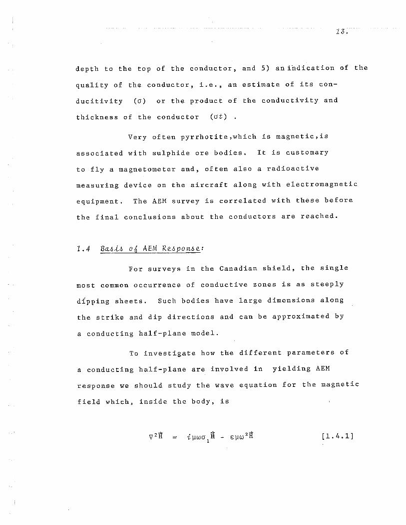
1.4 Ba1.:ii1.:i 06 AEM Re1.:ipon1.:ie ....•......•........•..... 13

1.5 Pne1.:ien.t S.ta.te 06 .the An.t .•.......•.......•...... 18

1.6 S.tandand In.tenpne.ta.tion Method ...............•.. 20

1.6.l Inphase and Quadrature Measuring Systems . 21

1.6.2 Quadrature systems ...................... 25

l .6.3 Transient (INPUT) system ................ 25

1.7 Objec..t 06 The1.:ii1.:i Re1.:ieanc.h ....................... 28

II. MOVEL MEASUREMENTS:

2.1 AEM Sy1.:i.tem1.:i Studied ..••......•...•.........•... 31

2.2 Quadna.tune and Tnan1.:iien.t Sy1.:i.tem1.:i ................ 33

2. 3 Model Conduc..ton1.:i ...•.•.•.•...........•.•........ 34

2.4 Mea1.:iuning Appana.tu1.:i .•..••.....•.•.•..•......•... 36

III. VERTICAL HALF-PLANE CONDUCTORS:

3.1 Smoothing 06 Signal1.:i ....•.....•..........•••.... 42

3. 2 Shape 06 Pno6ile1.:i ............................... 48

Page No.

3.2.1 Symmetrical Systems .................... 48

3.2.2 Unsymmetrical Systems .................. 51

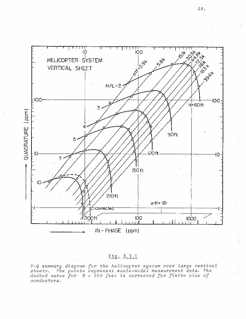
3. 3 Su.mmaJI.y ViagJI.am.o . . . . . . . . . . . . . . . . . . . . . . . . . . . . . . 5?

3.4 VependenQe an Re.opon.oe Pall.ametell. ... ........... 62

3.4.1 Ratio of Inphase and Quadrature Responses . . . . . . . . . . . . . . . . . . . . . . . . . . . . 62

3.4.2 Double-dipole Approximation ............ 6?

3.5 Fall-066 06 Re.opon.oe.o with Height ............. ?O

3. 6 Field Example.o ?5

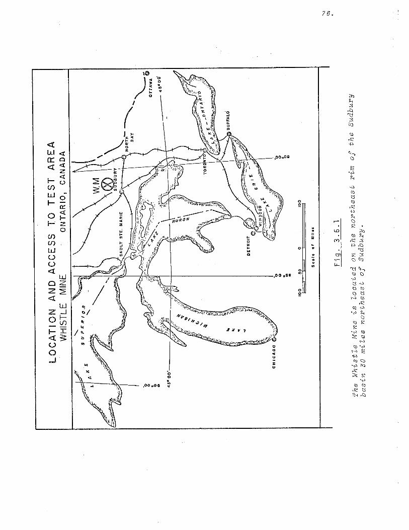
3. 6. 1

3. 6. 2

Whistle deposit 3.6.1.1 Dighem System ................ . 3.6.1.2 Whale-tail (Barringer)

system .................... . 3.6.1.3 Lockwood quadrature system ... . 3.6.1.4 McPhar quadrature system ..... .

Sturgeon 3.6.2.1 3. 6. 2. 2 3. 6. 2. 3

Lake Ore Body ................ . Scintrex HEM-701 ............. . McPhar quadrature system Lockwood quadrature system ....

?5

?5

80 83

86

92

92

95 96

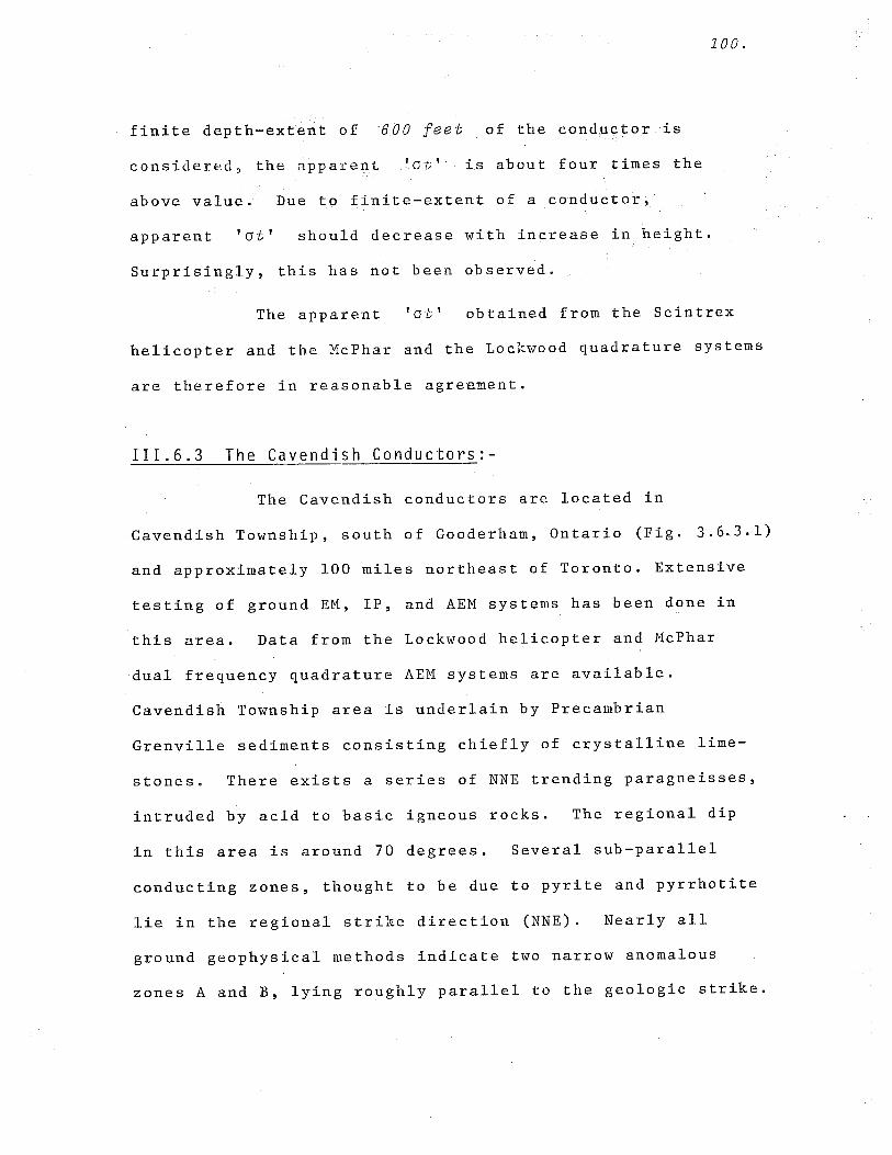
3.6.3 Cavendish Conductors ................... 100

3.6.3.l Lockwood helicopter system .... 102 3.6.3.2 McPhar quadrature system ...... 105

IV. FLAT-LYING CONVUCTORS:

4.1 SQale-madel Meahull.ement Vata ................. 111

4.1.l Shape of Profiles ..................... 111

4.1.1.1 Symmetrical systems .......... 111 4.1.1.2 Unsymmetrical systems ......... 114

4. 1 . 2 Magnitude of Responses 119

4.2. Field Example.o ................................ '12?

Page No.

V. ATTITUVE OF CONVUCTORS:

5. 1 Dipping Halfi-Plane-0 139

5 . 1 . 1 Symmetrical Systems ................... 139

5.1 .2 Unsymmetrical Systems .....•........... 142

5.1.3 Field Examples ......................... 150

5.Z Efifiec..t ofi S.tJiik.e Angle-0 ....................... 155

VI. CONDUCTORS OF LIMITED EXTENT:

6 • 1

6. z Vep.th-Ex.ten.t

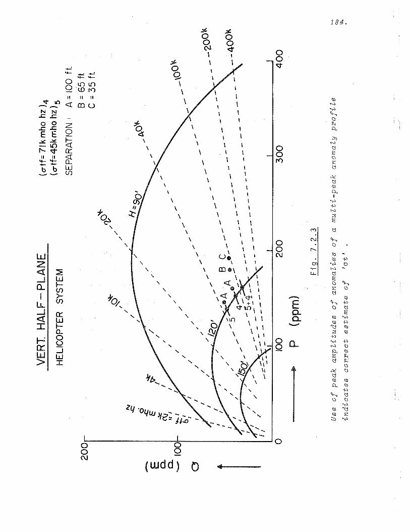
S.tJiik.e -Ex.ten.t

163

167

6 . 3 End En fi ec..t • • • • . • • • • • • . • • . • • • • • • • • • • • . • • • • • • • • • 1 7 2

VII. STUDY OF SPECIAL CASES:

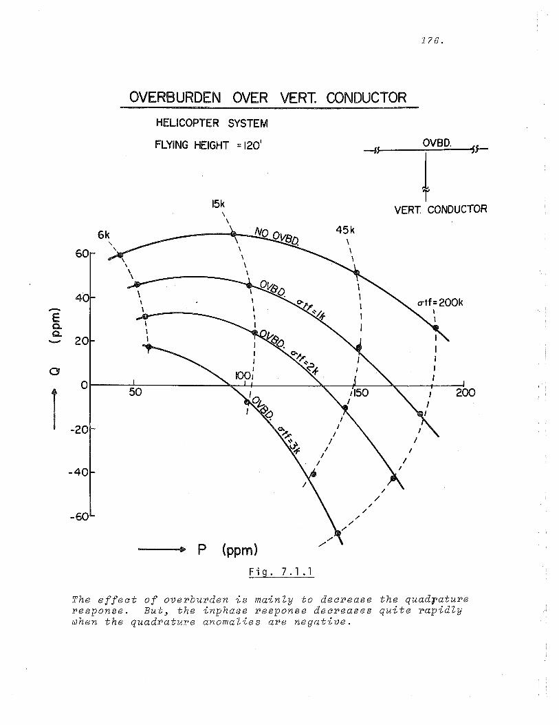
7.1 OveJibuJiden 175

7.Z Two PaJiallel Conduc..toJL-0 ....................... 180

7.3 Paoli Conduc..toJL-O SuJLJiounding a Good Conduc.to!L . . . . . . . . . . . . . . . . . . . . . . . . . . . . . . . . . . . . . 185

VIII. CONCLUSIONS: ................................ 189

APPENDIX 196

000000

1.

I I INTRODUCTION

I. 1 What~~ an AEM Sy~tem?

An airborne electromagnetic (AEM) prospecting

system is used for the detection of subsurface bodies which

are electrically conducting. It consists usually of a

transmitting coil and a receiving coil flown by an aircraft.

A controlled time-varying magnetic field is produced by the

transmitter. Most often the frequency of the transmitting

current is in the range 100-4000 hz. A component of the

field is then recorded at a point separated from the source,

by measuring the emf induced in the receiving coil.

The transmitter can be thought of as having a

dipole type alternating magnetic field. If a conducting

zone is in the vicinity, the source field will cut it, and

induced or eddy currents will flow inside the conductor in

closed loops more or less normal to the direction of the

magnetic field. These eddy currents, in turn, will

generate their own magnetic field. Thus at any point, the

total magnetic field is composed of a primary field due to

the source, and a secondary field due to the eddy currents

induced in the conducting zone. This secondary field lags

behind the primary field. Its amplitude is dependent upon

the frequency of the source current and the conductivity

distribution of the body. Since the secondary field is

2.

extremely small compared to the primary field, the primary

field at the receiver must be separated out somehow and

only the secondary field measured. Measurements made using

simple alternating fields are known as 'frequency-domain'

measurements; where a complex waveform or transient time­

variation is employed the measurements are said to be made

in the 'time-domain'.

I.Z Aetual AEM Sy~tem~:

In several actual 'frequency domain' AEM systems,

the inphase (P) and quadrature (Q) components of the

secondary field are measured with respect to the primary

field. These quantities are recorded continuously as the

aircraft flies along survey lines. They are referred to

as inphase (P) and quadrature (Q) responses or anoma-

lies, respectively. We obtain the spatial distribution

of these anomalies along the flight line. Magnitudes of

these anomalies are usually expressed in parts per million

(ppm) of the primary field which, by definition, is

totally inphase.

I. 2. 1 'Rigid-Boom' Systems:-

The most straightforward method of separating

the secondary and primary field strengths is to have the

transmitter and the receiver coils rigidly coupled so that

3.

the primary field is stable. These systems are known as

the 'rigid-boom' systems. A change in the coil-separation

of one part in a hundred thousand causes a change of

30 ppm in the inphase response. Presently, a sensitivity

of a few parts per million has been achieved in these

systems.

'Rigid-boom' systems are of three kinds depending

on how the tLansmitter and receiver coils are mounted. In

the most common kind of the 'rigid-boom' systems the coils

are separated by a distance of 20-30 feet and are housed

in a large bird which is towed by a helicopter by means of

a long cable (Fig. 1.2.la). The coils are vertical* and

coaxially oriented, the axis being directed along the line

of flight. This is known as the helicopter system (HEM).

Th~ helicopter flies at a normal height of 200 feet 3

and the bird trails at a height of about 100 feet . The

distance between the transmitter and receiver coils is very

small compared to the flight height of the bird. Because

of the small dimensions of the coil-separation

and the bird-height these systems are, in a rather loose

term, known as 'small-scale' systems.

* Coil configurations are usually described by stating the orientation of the plane in which the winding lies, although this is more ambiguous than describing the orientation of the axes.

4.

IOOft.

:+ --&

I· , ~ 3ott ·I h:::IOOft.

(a) HELICOPTER TOWED (BOOM) (b) HELICOPTER FIXED-FRAME {BOOM)

~2.ft. ~

h:::200ft.

{c) WING-TIP (BOOM)

L, 4 k BARRINGER 385

1

2401

4501

LOCKWOOD 4201

2301

4501

McPHAR 2001

3251

450'.

(d) TOWED~ BIRD

Fig. 1.2.1

h

Airborne eZeotromagnetic systems and their approximate

dimensions.

5.

Several of these systems are in use at the present

time: Scintrex HEM-701, Lockwood LHEM 200/300, Dighem

(main coaxial), Barringer HEM and Sander HEM systems. The

frequency employed in the systems is usually 900-1000 hz.

The Lockwood LHEM system has a choice of a high frequency

of 4000 hz besides the normal frequency of 1000 hz

Typical inphase and quadrature anomalies for a large,

outcropping conductor are around 200 ppm and 100 ppm

respectively,. for a normal flight height of the helicopter.

A noise level of as little as

in these systems.

3-10 ppm is often achieved

Besides the main coaxial receiver coil, the Dighem

system uses two more receiver coils which are null coupled

(Fig. 1.2.2). This means that the primary field cutting

these receiver coils is zero. The horizontal receiver coil

is known as the whale-tail receiver, and the vertical

receiver coil is known as the fish-tail receiver. The

Barringer HEM system also has a provision to use a whale­

tail receiver.

In another type of the 'rigid-boom' systems, the

transmitter and receiver coaxial coils are mounted on a

structure attached to the frame of a helicopter or a fixed

wing aircraft. The axes of the coils are in line with the

flight direction (Fig. 1.2.lb). Separation between the

coils is 50-83 feet Normal flying height is 150-175

feet. The frequency employed is around 400 hz The

3 RECEIVER COILS

DIGHEM SYSTEM

Fig. 1.2.2

6.

TRANSMITTER COIL (918 hz)

Schematic of the muZticoiZ receivers of the Dighem

helicopter towed system (Fraser, 19?2).

?.

anomalies obtained aregreater than those in the helicopter

systems. Typical noise level is 20-50 ppm. The Texas

Gulf Sulfer-Varian, Canadian Aero Service Canso, and

Newmont-Aero Service are the three existing systems.

A third kind of the 'rigid-boom' systems uses two

vertical coplanar coils as the transmitter and receiver,

mounted on the wing-tips of a small fixed wing aircraft

(Fig. 1.2.lc). The axes of the coils are parallel to the

line of flight. These systems are known as wing-tip systems.

The separation between the transmitter and receiver is

62 feet for an Otter aircraft. The aircraft flies at a

normal height of 150-200 feet . The frequency employed is

320 hz. The coil separation and height of the coil system

above ground surface are larger than those of the helicopter

systems. These are called 'medium-scale' systems and the

anomalies are higher than those obtained by the helicopter

systems. The noise level is 20-50 ppm . A few of these

systems which are presently in use are the Geoterrex Otter,

Scintrex Rio Mullard Otter, and Canadian Aero Otter systems.

I.2.2 Quadrature Systems:-

In contrast to the two component measuring 'rigid­

boom' systems, there exist a kind of system in which only

the quadrature components of the secondary field are

measured at two different frequencies. These systems are

8.

known as dual frequency qHadrature systems, or simply,

quadrature systems. Because the inphase components are

not utilized, the stability requirements in the relative

positioning of the receiver and transmitter coils are very

much relaxed. The transmitter may be a big loop wrapped

around the wings and tail of the aircraft. The receiver

is towed in a bird by means of a long cable. Systems

using the receiver on a bird, towed behind the aircraft,

are generally known as towed bird systems (Fig. 1.2.ld).

The horizontal and vertical separations between the trans-

mitter and receiver are a few hundred feet.

flies at a normal height of about 450 feet.

The aircraft

Due to the

greater dimensions of these systems, they are often called

'large-scale' systems. Two quadrature systems exist in

the industry: one is the Lockwood LEM 200 and the other

is the McPhar F-400. The Lockwood system employs a

horizontal coil as the transmitter, and a vertical coil,

with its axis along the line of flight, as the receiver.

The orientations of the coils of the McPhar system are

just the opposite. It has a vertical coil as the trans-

mitter and a horizontal coil as the receiver. The horizontal

and vertical separations of the Lockwood system are about

420 feet and 230 feet , and of the McPhar system are

about 200 feet and 325 feet, respectively. The

frequencies of the Lockwood system are 400 hz and

2300 hz, and those of the McPhar system are 340 hz

1O7 1 hz. The anomalies obtained in the field are

typically a few thousand ppm . The noise level is around

500 ppm.

I.2.3 Transient (Input) System:-

In all the systems already discussed the

measurements are made in the 'frequency-domain'. Only in

the Barringer INPUT system are the measurements made in

the 'time-domain'. This is a towed bird system of the

sta1 <lard geometrical configuration. The coil system

9.

con[>ists of a horizontal transmitter coil, and a vertical

rec~iver coil with its axis along the line of flight.

This system resembles the Lockwood quadrature system.

The transmitter coil is energized with what is essentially

a 'pulse current in the form of half of a sine curve. In

the absence of any conductor, a sharp transient emf

proportional to the time derivative of the magnetic field

is produced at the receiver in the form of half of a

cosine curve (Fig. 1.2.3). When a conductor is present,

however, the sudden change in the primary magnetic field

intensity will induce in it a flow of current which will

slowly decay, and will, through its secondary field induce

an emf in the receiver after the primary field has

ceased. The primary field is alternated in polarity and

lasts for 6.92 msec. It is repeated 144 times a second

H

a)

b)

c)

I.I msec 2.37 msec

I 2 3 4 5 6

Fig. 1.2.3

Principle of the time domain INPUT system: a) Primary current pulses alternate in polarity, the fundamental frequency is 144 Hz.; b) Emf due to primary field as detected in the bird; c) Emf due to secondary field, as detected in the bird. The emf decay is sampled at six time intervals, centred at 0.26, 0.48, 0.75, 1.1, 1.57, and 2.10 msec after cessation of the primary pulse (Palacky, 1972).

10.

t

11.

as the aircraft flies, so that the signal is virtually

continuous. The decay curve is sampled six times after

cessation of the transmitting pulse. It should be noted

that it is not decay of the magnetic field but its time

derivative which is recorded, because a coil is used as

a receiver. The entire decay of the secondary field is

equivalent to 'frequency-domain' measurements over the

whole frequency spectrum.

I.3 What l~ an AEM Sy~tem U~ed Fon?

An AEM survey is employed as a very rapid means

of economically searching large, geologically potential

areas to detect sulphide ore bodies within the top few

hundred feet of the earth's surface. The objectives of an

AEM survey are somewhat more limited than, or are at least f

different from , those of a ground survey. The primary

objective in both cases is to discover zonesof sulphide

mineralization and to discriminate between different types

of conductors. Beyond this, a ground survey is usually

required to provide some information of the shape of the

conductive body and to pinpoint its position sufficiently

well so that a drill might be accurately aimed towards it.

This second objective is rarely required of an AEM survey.

The physical property of the sulphide deposit

which is responsible for its detection by AEM surveys is

the high electrical conductivity. Sulphide minerals

including those comprising the usual ores of copper,

nickel, lead and silver possess this common property.

12.

Most unweathered igneous and metamorphic rocks have very

low electrical conductivity, and they are essentially

insulating as far as AEM measurements are concerned. Hence,

the AEM system may produce distinct anomalies over elec­

trically conducting bodies.

It is well known, however, ( e.g. Paterson(l971))

that the electrical conductivities of sulphide ores overlap

those of several uneconomical but commonly occurring

geological materials, including soils, graphitic schists

and carbonaceous sediments, water filled fauks and shear

zones, swamps, etc. So, it is easy to comprehend that an

overabundance of anomalies may be obtained in an AEM

survey. It is therefore expected that the AEM systems

give some indication of the conductor's general charac­

teristics so that only those which offer reasonable promise

may need be further investigated. In many cases, sulphide

mineralized zones occur in the form of steeply dipping

sheet type bodies.

The information which could be obtained from

the AEM survey are: 1) the type of model which the

conductor resembles; 2) how long the conductor extends

in the strike direction; 3) the direction in which the

conductor dips and some idea of the dip angle; 4) the