JSS Journal of Statistical SoftwareOctober 2016, Volume 74, Issue 7. doi: 10.18637/jss.v074.i07

Imputation with the R Package VIM

Alexander KowarikStatistics Austria

Matthias TemplVienna University of Technology &

Statistics Austria

Abstract

The package VIM (Templ, Alfons, Kowarik, and Prantner 2016) is developed to ex-plore and analyze the structure of missing values in data using visualization methods,to impute these missing values with the built-in imputation methods and to verify theimputation process using visualization tools, as well as to produce high-quality graphicsfor publications.

This article focuses on the different imputation techniques available in the package.Four different imputation methods are currently implemented in VIM, namely hot-deckimputation, k-nearest neighbor imputation, regression imputation and iterative robustmodel-based imputation (Templ, Kowarik, and Filzmoser 2011). All of these methodsare implemented in a flexible manner with many options for customization. Furthermorein this article practical examples are provided to highlight the use of the implementedmethods on real-world applications.

In addition, the graphical user interface of VIM has been re-implemented from scratchresulting in the package VIMGUI (Schopfhauser, Templ, Alfons, Kowarik, and Prantner2016) to enable users without extensive R skills to access these imputation and visualiza-tion methods.

Keywords: missing values, imputation methods, R.

1. Introduction

Data sets often include missing values but most statistical methods available in softwarepackages can only be applied to complete data sets. The aim of this paper is not to providea thorough discussion of single versus multiple imputation; a comparison of both in practicecan be found, for example, in Gómez-Carracedo, Andrade, López-Mahía, Muniategui, andPrada (2014). However, some practical issues in this regard are also mentioned in this paper.In a typical statistical production process, the aim is often to generate one complete data set

2 Imputation with the R Package VIM

for further analysis by subject matter specialists, researchers or analysts. Therefore singleimputation is still of great importance. Typically, the data is handed from the data collectionsystem to the experts on imputation to perform imputation on the data, before the data isthen used by subject matter specialists and made available to researchers, analysts, and ispublished.On the other hand, if the estimation of the variance of certain parameters is of interest, thevariances might be underestimated using (single) imputed data sets since unique values arepredicted for missing values and thereby the uncertainty in the prediction is not reflected(Rubin 1987; Little and Rubin 2014). Multiple imputation methods are designed to reflectalso this uncertainty by imputing several values for each missing value, leading to a set ofimputed data sets. The variability between these imputations is then taken into account asit reflects the variance of the prediction. The variances of the estimators of interest are thenestimated on each imputed data set and these results are combined, e.g., using the formulasgiven in Rubin (1987).A wide range of single imputation algorithms are available, e.g., in the R (R Core Team2016) packages yaImpute (Crookston and Finley 2008), missMDA (Josse and Husson 2016),CoImp (Lascio and Giannerini 2016), as well as multiple imputation methods, e.g., in theR packages mice (van Buuren and Groothuis-Oudshoorn 2011), AmeliaII (Honaker, King,and Blackwell 2011), mix (Schafer 2015), missMDA (Josse and Husson 2016), Hmisc (Harrell2015), missForest (Stekhoven and Bühlmann 2012). These packages are well-known andwidely used and for many applications they give excellent results in their field of application.In many fields the data contains variables of different distributions. For example, data fromofficial statistics, social statistics or econometrics consists of a variety of differently scaledvariables. To give an example, demographic variables like gender, age, region, economicstatus or branch, citizenship, household size, etc., are present in data along with variableson income and income components. For imputing missing values in one variable, all thesevariables of different scales might be used since they provide essential information.However, most of these packages are not designed to deal with a mix of continuous, semi-continuous, categorical and count data. Note that for the predictive mean matching method(van Buuren and Groothuis-Oudshoorn 2011) in the package mice, treating semi-continuousvariables as continuous variables may not necessarily give worse results. Regarding the mixof variables, an exception is the package mi (Su, Gelman, Hill, and Yajima 2011) which usesa two-part model to deal with semi-continuous variables and which supports a mix of semi-continuous, continuous and categorical variables, further it allows for multiple imputation.In addition, some of the implemented popular methods cannot be found in those packages, likehot-deck imputation, robust regression imputation or k nearest neighbor (kNN) imputationusing generalized distance functions. An exception is the package yaImpute (Crookston andFinley 2008) which has excellent features for kNN methods for continuous scaled variables.Another package, rrp (Iacus and Porro 2007), includes nearest neighbor hot-deck imputationusing a random recursive partitioning dissimilarity matrix. Random hot-deck imputation isalso available in an SPSS (IBM Corporation 2015) implementation (Myers 2011) and in SAS(SAS Institute Inc. 2013) with SUDAAN’s (Research Triangle Institute 2008) SAS-callablePROC HOTDECK (Izrael and Battaglia 2013). However, these packages are not designed to dealwith generalized distances, which should be used when dealing with a mix of differently scaledvariables.

Journal of Statistical Software 3

In addition, the data sets are often of moderate or large size and fast imputation algorithmsare needed. Especially, the packages for multiple imputation based on MCMC methods maynot provide feasible solutions in terms of computational speed for large data sets.Another important issue in practice is how imputation methods deal with outliers in con-tinuous variables. The literature on robust statistics clearly shows that methods based onnon-robust estimators are highly influenced by outliers (see, e.g., Maronna, Martin, and Yohai2006). The imputation model can be highly influenced by outliers and the imputed valuesmay deviate from the majority of the data, and can itself be outliers. As a result, the variancesof estimators of imputed data can become arbitrary large but also point estimates might behighly influenced by non-robust imputations of continuous variables (Templ et al. 2011).The R package VIM (Templ et al. 2016), available from the Comprehensive R Archive Network(CRAN) at http://CRAN.R-project.org/package=VIM, provides solutions for mixed scaledvariables, large data sets and data sets including outliers. It includes several improvementswith respect to the robustness of the parameter estimation of models to impute missing values.This functionality is included in the EM-based imputation method (see Section 4).In addition, the package VIM includes two single imputation methods, (random and se-quential) hot-deck imputation and kNN imputation using a generalized distance function toconsider mixed scaled variables in the data set to impute, and user-specified aggregationfunctions.The only method in package VIM that supports multiple imputation is the (robust) EM-based imputation method in Section 4. It works differently from other well-known methodsthat draw values for imputations from their conditional distributions by Markov chain MonteCarlo (MCMC) techniques (see e.g., van Buuren and Groothuis-Oudshoorn 2011; Schunk2008). Such techniques need longer to converge and are typically more demanding in termsof computer resources. The implemented EM-approach has advantages regarding the speedof “convergence” since expected values are used for imputations and only in a last iterationvariability is added to the model (see Section 4 and Templ et al. 2011 for details).Typically, multiple imputation methods such as those available in packages mice or mixfollow a fully conditional specification approach, where iteratively one variable is selected asthe response and all other variables serve as predictors. With package VIM also a model foreach variable can be specified. Note that package mi includes this additional feature as well.The package VIM also supports the visual exploration of the data by several visualizationmethods that have been adapted to work with and show the structure of missing values.Further details on these methods can be found in Templ, Alfons, and Filzmoser (2012).To visualize the structure of missing values and to learn about these structure is highlyrecommended before missing values are imputed. In addition, the same visualization featurescan be used to visualize the structure of imputed values to get an impression if the imputedvalues follows the main structure of the (observed) data.All methods can be applied by using the point-and-click graphical user interface (availablein the package VIMGUI; Schopfhauser et al. 2016) that has been newly implemented fromscratch. In addition, objects from the package survey (Lumley 2016, 2004) can be imputed.This is especially useful in the area of survey methodology. However, this contribution doesnot focus on the graphical user interface.The methods in package VIM also have some limitations. There is no direct support forlongitudinal data. For such data, package AmeliaII (Honaker et al. 2011) can be mentioned

4 Imputation with the R Package VIM

that is designed to impute cross-sectional data and time series. In VIM longitudinal data canonly be combined by rows (e.g., using rbind()) before imputation to consider a longitudinalaspect in data imputation. In addition the MI approach implemented in the function irmi isnot based on MCMC methods and thus coverage rates might theoretically be biased.

The four implemented imputation methods are described in the following sections, where eachsection contains theoretical background, implementation details and an example of applicationfor each method. Section 2 describes the hot-deck imputation function of the package VIM.Since the main advantage of this implementation is computational speed, also informationon the computational time for a large data set is given. The kNN imputation method is thefocus of Section 3. Attention is given to the description of the generalized distance functionand an application with a user-defined aggregation function is presented. In Section 4, theusage and implementation of iterative robust model-based imputation is shown on practicalapplications. Here, user-defined models are specified for each variable including missing valuesin order to show the flexibility of the implemented functions. Section 5 shows how to imputea single variable by regression imputation using the formula interface. Section 6 concludes bygiving an outline on the broad range of applications where package VIM can be used.

2. Hot-deck imputation

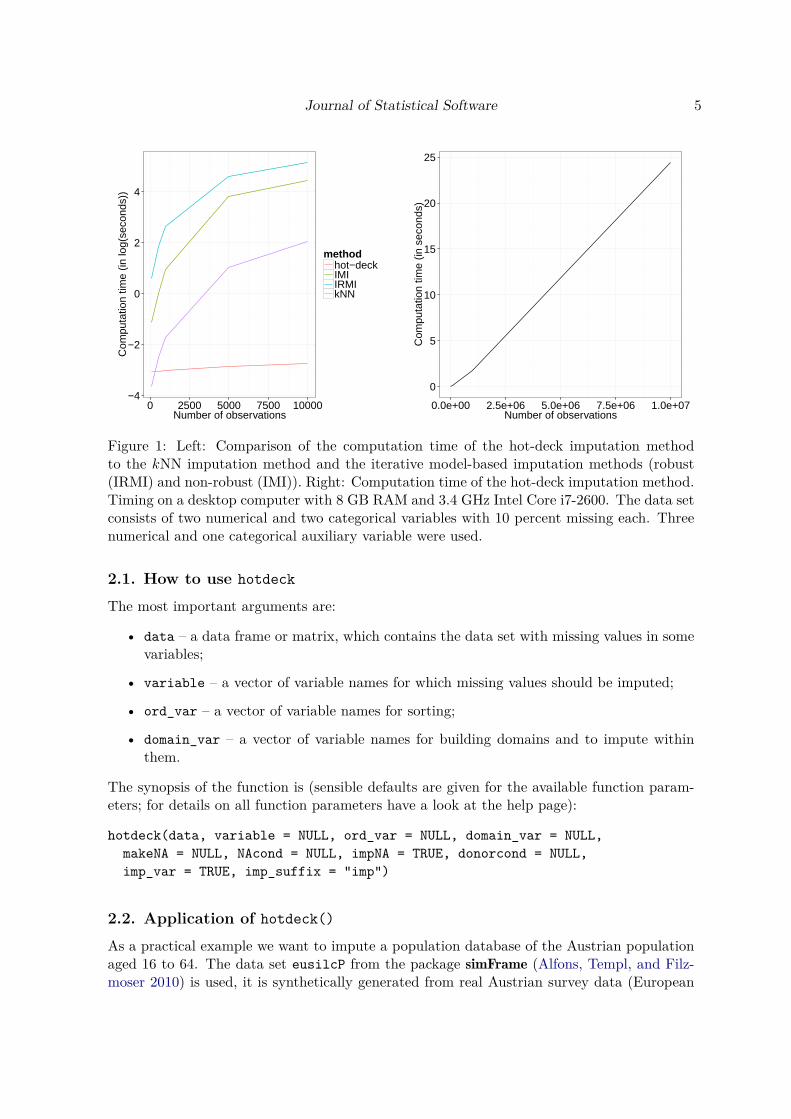
Hot-deck imputation dates back to the days when data sets were saved on punch cards,the hot-deck referring to the “hot” staple of cards (in opposite to the “cold” deck of cardsfrom the previous period). This very heuristic approach was later also studied theoretically,e.g., by Sande (1983), Ford (1983) and Fuller and Kim (2005). Most of the time, hot-deckimputation refers to sequential hot-deck imputation, meaning that the data set is sorted andmissing values are imputed sequentially running through the data set line (observation) byline (observation). Nowadays, methods with better theoretical properties are available, butthe method is still quite popular due to its simplicity and speed. In a lot of cases the quality ofimputation with hot-deck imputation can be similar to nearest neighbor imputation, howeveras seen in Figure 1 it is much faster. The speed disadvantage of the nearest neighbor approachis mainly due to computing distances between all observations with missing values and thepossible donor observations to find the k nearest neighbors (see Section 3 for more details).Therefore hot-deck imputation is very well suited for imputation of big data sets as seen inFigure 1. The computation speed of the hot-deck method is much faster than kNN (describedin Section 3) and the model-based methods (described in Section 4). For this small simulation,eight variables are synthetically produced, where ten percent of the values of four variablesare set to missing. One variable determines the domain and three variables are used forordering the data within the hot-deck procedure. For example, for 10,000 observations, themodel-based methods need around 150 seconds while hot-deck is below 0.1 seconds (compareFigure 1). The computational time increases linearly with the number of observations in thedata sets and it is still below 26 seconds for a data set with 10,000,000 observations (seeFigure 1).

The function hotdeck() is the implementation of the popular sequential and random hot-deck algorithm with the option to use it within a domain. It is optimized for usage on bigdata sets by using the R package data.table (Dowle, Srinivasan, Short, and Lianoglou 2015).

Journal of Statistical Software 5

−4

−2

0

2

4

0 2500 5000 7500 10000Number of observations

Com

puta

tion

time

(in lo

g(se

cond

s))

methodhot−deckIMIIRMIkNN

0

5

10

15

20

25

0.0e+00 2.5e+06 5.0e+06 7.5e+06 1.0e+07Number of observations

Com

puta

tion

time

(in s

econ

ds)

Figure 1: Left: Comparison of the computation time of the hot-deck imputation methodto the kNN imputation method and the iterative model-based imputation methods (robust(IRMI) and non-robust (IMI)). Right: Computation time of the hot-deck imputation method.Timing on a desktop computer with 8 GB RAM and 3.4 GHz Intel Core i7-2600. The data setconsists of two numerical and two categorical variables with 10 percent missing each. Threenumerical and one categorical auxiliary variable were used.

2.1. How to use hotdeck

The most important arguments are:

• data – a data frame or matrix, which contains the data set with missing values in somevariables;

• variable – a vector of variable names for which missing values should be imputed;

• ord_var – a vector of variable names for sorting;

• domain_var – a vector of variable names for building domains and to impute withinthem.

The synopsis of the function is (sensible defaults are given for the available function param-eters; for details on all function parameters have a look at the help page):

hotdeck(data, variable = NULL, ord_var = NULL, domain_var = NULL,makeNA = NULL, NAcond = NULL, impNA = TRUE, donorcond = NULL,imp_var = TRUE, imp_suffix = "imp")

2.2. Application of hotdeck()

As a practical example we want to impute a population database of the Austrian populationaged 16 to 64. The data set eusilcP from the package simFrame (Alfons, Templ, and Filz-moser 2010) is used, it is synthetically generated from real Austrian survey data (European

6 Imputation with the R Package VIM

Union Statistics on Income and Living Conditions; EU-SILC). The data set is enlarged bysampling 5.5 million observations with replacement from the data set with 39 thousand obser-vations. The data set is split by federal state (region) and gender by using these variablesas domain variables. The numeric variables are equalized household income (eqIncome), ageand the number of persons in a household (hsize) and are used for sorting the data set. Tenpercent missing values are generated in the person’s economic status (ecoStat), citizenshipand three income components (py010n, py050n and py090n). Detailed information about thedata set and the variables can be found in the help file of eusilcP in the package simFrame.Finally, hot-deck imputation is applied to the data set ordered by equalized income, age andhousehold size within the domains constructed by region and gender. The imputed data setis stored in object popImp and the computation time is given for these approximately half amillion imputations

R> library("VIM")R> data("eusilcP", package = "simFrame")R> eusilcP <- eusilcP[eusilcP$age > 15 & eusilcP$age < 65, ]R> pop <- eusilcP[sample(1:nrow(eusilcP), 5.5e6, replace = TRUE),+ c("region", "gender", "hsize", "age", "eqIncome", "ecoStat",+ "citizenship", "py010n", "py050n", "py090n")]R> dim(pop)

[1] 5500000 10

R> for (v in c("ecoStat", "citizenship", "py010n", "py050n", "py090n")) {+ pop[sample(1:nrow(pop), round(nrow(pop)/10), replace = TRUE), v] <- NA+ }R> system.time(popImp <- hotdeck(pop, ord_var = c("eqIncome", "age",+ "hsize"), domain_var = c("region", "gender")))

user system elapsed10.60 0.44 11.08

3. k nearest neighbor imputationSimilar to the hot-deck method, the k nearest neighbor method is based on donor observation.An aggregation of the k values of the nearest neighbors is used as imputed value. The kindof aggregation depends on the type of the variable.The distance computation for defining the nearest neighbors is based on an extension of theGower distance (Gower 1971), which can now handle distance variables of the type binary,categorical, ordered, continuous and semi-continuous. The distance between two observationsis the weighted mean of the contributions of each variable, where the weight should representthe importance of the variable. Therefore the distance between the ith and the jth observationcan be defined as

di,j =∑p

k=1wkδi,j,k∑pk=1wk

, (1)

Journal of Statistical Software 7

where wk is the weight and δi,j,k is the contribution of the kth variable.For continuous variables the absolute distance divided by the total range is used

δi,j,k = |xi,k − xj,k|/rk , (2)

where xi,k is the value of the kth variable of the ith observation and rk is the range ofthe kth variable. Ordinal variables are converted to integer variables and then the absolutedistance divided by the range is computed. The categories are therefore treated as if theywere equidistant; this can be changed by manually converting the ordinal variables to integervariables.For nominal and binary variables a simple 0/1 distance is used

δi,j,k ={

0 if xi,k = xj,k ,

1 if xi,k 6= xj,k .(3)

Another special type of variables are semi-continuous variables, consisting of a continuouslydistributed part and probability mass at one point. An example for such a variable might bean income component, which is 0 for some observations and continuously distributed in theremaining observations. The contributions for semi-continuous variables are computed as amixture of the contribution for nominal and continuous variables

δi,j,k =

0 if xi,k = sk ∧ xj,k = sk ,

1 if xi,k 6= sk ∧ xj,k = sk ,

1 if xi,k = sk ∧ xj,k 6= sk ,

|xi,k − xj,k|/rk if xi,k 6= sk ∧ xj,k 6= sk ,

(4)

where sk is the special value for the kth variable, e.g., the 0 in the income variable example.As described above, all δi,j,k are in [0, 1], as a consequence the computed distances di,j betweentwo observation are also inside this interval.The distance computation is implemented in C++ with usage of the R package Rcpp (Eddel-buettel, François, Allaire, Chambers, Bates, and Ushey 2011).The second important part of this method is the aggregation of the k values to one imputedvalue. For continuous variables the default is the median, but also other statistics are pos-sible e.g., the arithmetic mean. For categorical variables the default method is to use thecategory with the most occurrences in the k values, if this results in a tie, a category fromthe tied categories is randomly drawn (function maxCat()). A second implemented methodof aggregation is to sample the category from the categories in the k nearest neighbors withprobabilities equal to the occurrences in the k values (function sampleCat()).

3.1. How to use kNN()

The most important arguments are:

• dist_var – a vector of variable names to be used for calculating the distances;

• weights – a numeric vector containing a weight for each distance variable;

8 Imputation with the R Package VIM

• numFun – a function for aggregating the k nearest neighbors in case of a numericalvariable, defaults to the median;

• catFun – a function for aggregating the k nearest neighbors in case of a categoricalvariable, defaults to the function maxCat();

• addRandom – a Boolean variable if an additional variable containing only random num-bers is added to avoid multiple selection of the same donor;

• useImputedDist – a Boolean variable if an imputed value should be used for distancecalculation for imputing another variable. Be aware that this results in a dependencyon the ordering of the variables;

• weightDist – a Boolean variable if the inverse of the distances of the k nearest neigh-bours should be used as weights in the aggregation step.

The full synopsis (including sensible defaults) of the function is:

kNN(data, variable = colnames(data), metric = NULL, k = 5,dist_var = colnames(data), weights = NULL, numFun = median,catFun = maxCat, makeNA = NULL, NAcond = NULL, impNA = TRUE,donorcond = NULL, mixed = vector(), mixed.constant = NULL, trace = FALSE,imp_var = TRUE, imp_suffix = "imp", addRandom = FALSE,useImputedDist = TRUE, weightDist = FALSE)

The method is implemented in a sophisticated manner so that not the whole distance matrixhas to be calculated but only distances for observations including missing values, and vari-ables which are chosen by the variable argument. Thus the implementation in VIM is alsoapplicable for reasonably large data sets. However, computation of the distance is in any casemore time-consuming than the hot-deck method (Figure 1).

3.2. Application of kNN

Again we use the EU-SILC data set for showcasing the imputation method. As mentionedbefore the function kNN() is versatile in handling different variable types in the distancefunction, but it is also possible to use aggregation functions for different variable types. For asemi-continuous variable an aggregation function might look like the function medianMixed().It returns 0 with a probability equivalent to the relative frequency of 0 in the k nearestneighbors and the median of the non-0 observations otherwise.Again missing values are introduced. The user-defined aggregation function (medianMixed())is given in the following code snippet and kNN() is applied where all variables defined in theobject samp are used for distance calculation. In this case we do not use the function argumentweights to weight the variables for distance calculations. However if the importance of thevariables is considered to differ substantially, this can be handled by this argument.

R> data("eusilcP", package = "simFrame")R> eusilcP <- eusilcP[eusilcP$age > 15 & eusilcP$age < 65, ]R> samp <- eusilcP[sample(1:nrow(eusilcP), 14e3, replace = FALSE),+ c("region", "gender", "hsize", "age", "eqIncome", "ecoStat",

Journal of Statistical Software 9

+ "citizenship", "py010n", "py050n", "py090n")]R> for (v in c("ecoStat", "citizenship", "py050n", "py090n", "py010n")) {+ samp[sample(1:nrow(samp), round(nrow(samp) / 10),+ replace = TRUE), v] <- NA+ }R> medianMixed <- function(x) {+ nr <- sum(x == 0) / length(x)+ out <- sample(c(0, 1), size = 1, prob = c(nr, 1 - nr))+ if (out == 0 || nr == 1)+ return(0)+ else+ return(median(x[x != 0]))+ }R> sampImp <- kNN(samp, dist_var = c("eqIncome", "age", "hsize", "region",+ "gender"), k = 5, numFun = medianMixed)

Time difference of 39.34293 secs

The output (object sampImp) can be further analyzed using the visualization features of VIM(Templ et al. 2012). (The imputation took about 39 seconds).

4. Iterative robust model-based imputationThis iterative regression imputation method is described in detail in Templ et al. (2011). Ineach step of the iteration (inner loop), one variable is used as a response variable and theremaining variables serve as the regressors. The procedure is repeated until the algorithmconverges (outer loop). The data can consist of a mix of binary, categorical, count, continuousand semi-continuous variables, appropriate regression methods are selected internally by thealgorithm. Robust regression using MM-estimation (Maronna et al. 2006) is used by defaultto get reliable results even if the data contains outliers. This method is most useful to getreliable imputations in an automated manner. However, if the users are trained in regressionmodeling, a model for each variable can also be specified.

4.1. How to use irmi()

The most important arguments are:

• robust – a Boolean variable to enable or disable robust regression;

• step – a Boolean variable to enable or disable a step-wise (stepAIC) selection of regres-sors in each iteration;

• mixed – column index of the semi-continuous variables:

• count – column index of the count variables;

• modelFormulas – a named list with the name of variables for the right-hand side of theformulas. The list must contain a right-hand side formula for each variable with missing

10 Imputation with the R Package VIM

values and it should look like list(y1 = c("x1", "x2"), y2 = c("x1", "x3")) iffactor variables for the mixed variables should be created for the regression models;

• mi – the number of multiple imputed values.

The latter two arguments are important for selecting the correct regression method, whichis done within the algorithm in an automatized manner hidden from the user. If the datacontains semi-continuous or count variables, this must be specified while the algorithm detectsthe correct distribution for all other types (continuous, binary, categorical).The full call of the function is:

irmi(x, eps = 5, maxit = 100, mixed = NULL, mixed.constant = NULL,count = NULL, step = FALSE, robust = FALSE, takeAll = TRUE, noise = TRUE,noise.factor = 1, force = FALSE, robMethod = "MM", force.mixed = TRUE,mi = 1, addMixedFactors = FALSE, trace = FALSE, init.method = "kNN")

4.2. Application of irmi()

The data set ses from the package laeken (Alfons and Templ 2013) is a synthetically generateddata for the Austrian structural earnings survey. It contains variables of various kinds. Tenpercent of the following four variables are set to missing:

• location – the NUTS3 region in Austria;

• earningsMonth – the gross earnings in the reference month;

• earningsOvertime – the gross earnings related to overtime;

• overtimeHours – the number of paid overtime hours in the reference month.

R> data("ses", package = "laeken")R> sesOrig <- sesR> variables <- c("earningsMonth", "earningsOvertime", "overtimeHours",+ "location")R> for (v in variables) {+ ses[sample(1:nrow(ses), round(nrow(ses) / 10), replace = TRUE), v] <- NA+ }R> modelFormulas <- list(earningsMonth = c("earningsHour", "fullPart"),+ earningsOvertime = c("overtimeHours", "earningsHour"),+ overtimeHours = c("earningsOvertime", "shareNormalHours"),+ location = c("NACE1", "size"))R> sesImp <- irmi(ses, init.method = "median",+ mixed = c("overtimeHours", "earningsOvertime"),+ modelFormulas = modelFormulas)R> sesImpRob <- irmi(ses, init.method = "median",+ mixed = c("overtimeHours", "earningsOvertime"), robust = TRUE,+ modelFormulas = modelFormulas)

Journal of Statistical Software 11

The computation is done with non-robust regression methods and robust regression methods;the former took five seconds and the latter took 16 seconds to complete. Diagnostics canagain be run by using the visualization features of VIM, see Templ et al. (2012).

5. Individual regression imputationThis method is based on using well-known regression models to impute missing values on a pervariable basis. For continuous variables a linear model is internally fitted with the functionlm() or robustly with the function lmrob() from the R package robustbase (Rousseeuw et al.2016). The functions glm() and glmrob() (again from the package robustbase) are usedwhen a family is specified. For ordinal variables the function multinom() from the R packagennet (Venables and Ripley 2002) is used.

5.1. How to use regressionImp

The most important arguments are:

• formula – model formula to impute one variable;

• robust – TRUE/FALSE indicating if robust regression should be used;

• family – family argument passed to glm() or glmrob(). The default value "AUTO" triesto select the correct model family automatically.

The full call of the function is:

regressionImp(formula, data, family = "AUTO", robust = FALSE,imp_var = TRUE, imp_suffix = "imp", mod_cat = FALSE)

5.2. Application of regressionImp

The data set of the structural earnings survey of Austria is used again. Ten percent missingvalues are introduced in two variables earningsHour – the hourly earnings – and NACE1 – theeconomic branch. These two variables are imputed using a linear regression model for thefirst variable and multinomial regression for the second variable.

R> data("ses", package = "laeken")R> form1 <- earningsHour ~ location + size + economicFinanc ++ payAgreement + sex + age + education + occupation + contract ++ lengthService + overtimeHours + holiday + notPaid + earningsOvertime ++ paymentsShiftWork + earningsMonth + earningsR> form2 <- NACE1 ~ location + size + economicFinanc + payAgreement ++ sex + age + education + occupation + earningsR> for (v in c("earningsHour", "NACE1")) {+ ses[sample(1:nrow(ses), round(nrow(ses) / 10)), v] <- NA+ }R> ses <- regressionImp(form1, ses)R> ses <- regressionImp(form2, ses)

The two variables are now imputed and included in object ses.

12 Imputation with the R Package VIM

6. A short note on the graphical user interfaceThe R package VIMGUI implements a graphical user interface for the R package VIM. Theimputation methods described in this paper and the visualization techniques described inTempl et al. (2012) are accessible via an easy-to-use point and click user interface.Some of the additionally supported features of the graphical user interface are:

Import/Export: Import of .csv files with interactive selection of parameters for importing.The import and export of SPSS, SAS (XPORT format), Stata (StataCorp. 2015) andR binary files is supported. Objects of class ‘survey’, from the R package survey(Lumley 2016, 2004) for analyzing data from sample surveys, can be used as input forthe imputation process through the menu entry Survey where such survey objects canbe imported to VIMGUI and exported. Facilities to create a survey object are includedas well.

Scaling/Transformation: Standardization and/or transformation of continuous and semi-continuous variables.

Script: The results produced within the GUI are saved as commands in a separated file.This is useful to provide reproducibility.

Methods: A dozen of univariate, bivariate, multiple and multivariate diagnostic plots areavailable to evaluate the structure of missing values (∼ missing values diagnostics) andimputed values (∼ imputed values diagnostics).

As the graphical user interface is still under development, improvement to its functionalitycan be expected with future versions of the package.

7. ConclusionsThe VIM (and VIMGUI) package includes a comprehensive collection of imputation (andvisualization methods). Before imputation, the structure of missing values can be exploredusing the built-in visualization tools. Methods for the imputation of missing values are avail-able and special attention was given to efficient implementations of the methods.In summary, the package VIM can be widely applied since it

• can be used to impute incomplete data sets with continuous, semi-continuous, categor-ical, ordered-categorical, binary or count variables;

• is highly customizable by providing own functions and models;

• is optimized for large data sets, i.e., it includes efficient implementations of algorithmsusing the R packages Rcpp (Eddelbuettel et al. 2011) and data.table (Dowle et al. 2015);

• is possible to apply the imputation methods either to data frames or objects from thepackage survey;

• can be used by users with no experience in R via the package VIMGUI;

Journal of Statistical Software 13

• includes a lot of visualization features for analyzing the structure of missing values (herewe refer to Templ et al. 2012);

• even not shown in this paper, VIM include a lot of visualization features for analyzingthe imputed values. Imputations are highlighted in the plots, similar to the methods inTempl et al. (2012) where missing values are highlighted.

The packages VIM and VIMGUI are currently widely used around the world. The downloadstatistics for the R package downloads over one of many download mirrors – the RStudioserver – shows that the package has been downloaded more than 150 times a week over thelast two years (package updates also contribute to this number).

Session information

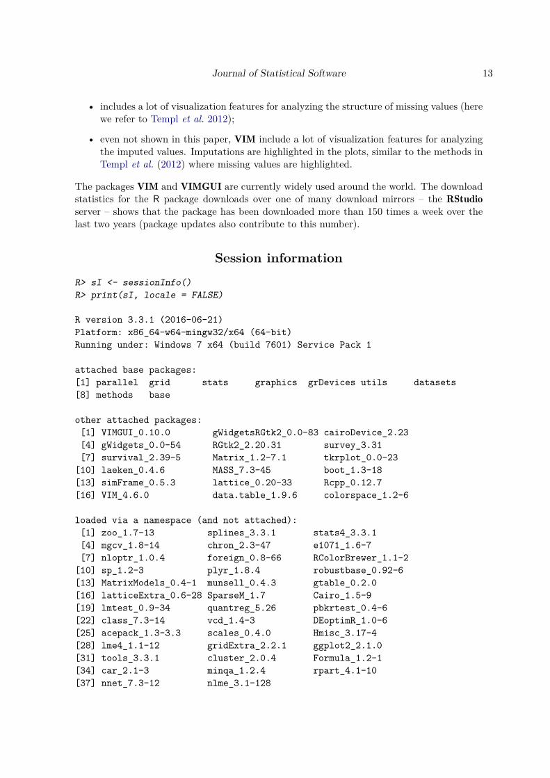
R> sI <- sessionInfo()R> print(sI, locale = FALSE)

R version 3.3.1 (2016-06-21)Platform: x86_64-w64-mingw32/x64 (64-bit)Running under: Windows 7 x64 (build 7601) Service Pack 1

attached base packages:[1] parallel grid stats graphics grDevices utils datasets[8] methods base

other attached packages:[1] VIMGUI_0.10.0 gWidgetsRGtk2_0.0-83 cairoDevice_2.23[4] gWidgets_0.0-54 RGtk2_2.20.31 survey_3.31[7] survival_2.39-5 Matrix_1.2-7.1 tkrplot_0.0-23

[10] laeken_0.4.6 MASS_7.3-45 boot_1.3-18[13] simFrame_0.5.3 lattice_0.20-33 Rcpp_0.12.7[16] VIM_4.6.0 data.table_1.9.6 colorspace_1.2-6

loaded via a namespace (and not attached):[1] zoo_1.7-13 splines_3.3.1 stats4_3.3.1[4] mgcv_1.8-14 chron_2.3-47 e1071_1.6-7[7] nloptr_1.0.4 foreign_0.8-66 RColorBrewer_1.1-2

[10] sp_1.2-3 plyr_1.8.4 robustbase_0.92-6[13] MatrixModels_0.4-1 munsell_0.4.3 gtable_0.2.0[16] latticeExtra_0.6-28 SparseM_1.7 Cairo_1.5-9[19] lmtest_0.9-34 quantreg_5.26 pbkrtest_0.4-6[22] class_7.3-14 vcd_1.4-3 DEoptimR_1.0-6[25] acepack_1.3-3.3 scales_0.4.0 Hmisc_3.17-4[28] lme4_1.1-12 gridExtra_2.2.1 ggplot2_2.1.0[31] tools_3.3.1 cluster_2.0.4 Formula_1.2-1[34] car_2.1-3 minqa_1.2.4 rpart_4.1-10[37] nnet_7.3-12 nlme_3.1-128

14 Imputation with the R Package VIM

References

Alfons A, Templ M (2013). “Estimation of Social Exclusion Indicators from Complex Surveys:The R Package laeken.” Journal of Statistical Software, 54(15), 1–25. doi:10.18637/jss.v054.i15.

Alfons A, Templ M, Filzmoser P (2010). “An Object-Oriented Framework for StatisticalSimulation: The R Package simFrame.” Journal of Statistical Software, 37(3), 1–36. doi:10.18637/jss.v037.i03.

Crookston NL, Finley AO (2008). “yaImpute: An R Package for kNN Imputation.” Journalof Statistical Software, 23(10), 1–16. doi:10.18637/jss.v023.i10.

Dowle M, Srinivasan A, Short T, Lianoglou S (2015). data.table: Extension of data.frame.R package version 1.9.6, URL https://CRAN.R-project.org/package=data.table.

Eddelbuettel D, François R, Allaire J, Chambers J, Bates D, Ushey K (2011). “Rcpp: SeamlessR and C++ Integration.” Journal of Statistical Software, 40(8), 1–18. doi:10.18637/jss.v040.i08.

Ford BL (1983). “An Overview of Hot-Deck Procedures.” Incomplete Data in Sample Surveys,2(Part IV), 185–207.

Fuller WA, Kim JK (2005). “Hot Deck Imputation for the Response Model.” Survey Method-ology, 31(2), 139.

Gómez-Carracedo MP, Andrade JM, López-Mahía P, Muniategui S, Prada D (2014). “A Prac-tical Comparison of Single and Multiple Imputation Methods to Handle Complex MissingData in Air Quality Datasets.” Chemometrics and Intelligent Laboratory Systems, 134,23–33. doi:10.1016/j.chemolab.2014.02.007.

Gower JC (1971). “A General Coefficient of Similarity and Some of Its Properties.” Biometrics,pp. 857–871. doi:10.2307/2528823.

Harrell F (2015). Hmisc: Harrell Miscellaneous. R package version 3.16-0, URL https://CRAN.R-project.org/package=Hmisc.

Honaker J, King G, Blackwell M (2011). “Amelia II: A Program for Missing Data.” Journalof Statistical Software, 45(7), 1–47. doi:10.18637/jss.v045.i07.

Iacus S, Porro G (2007). “Missing Data Imputation, Matching and Other Applications ofRandom Recursive Partitioning.” Computational Statistics & Data Analysis, 52(2), 773–789. doi:10.1016/j.csda.2006.12.036.

IBM Corporation (2015). IBM SPSS Statistics 23. IBM Corporation, Armonk, NY. URLhttp://www.ibm.com/software/analytics/spss/.

Izrael D, Battaglia MP (2013). “Weighted Sequential Hot Deck Imputation: SAS Macrovs. SUDAAN’s PROC HOTDECK.” Paper 213.

Josse J, Husson F (2016). missMDA: A Package for Handling Missing Values in MultivariateData Analysis. doi:10.18637/jss.v070.i01.

Journal of Statistical Software 15

Lascio F, Giannerini S (2016). CoImp: Copula Based Imputation Method. R package version0.3-1, URL https://CRAN.R-project.org/package=CoImp.

Little R, Rubin D (2014). Statistical Analysis with Missing Data. John Wiley & Sons.

Lumley T (2004). “Analysis of Complex Survey Samples.” Journal of Statistical Software,9(8), 1–19. doi:10.18637/jss.v009.i08.

Lumley T (2016). survey: Analysis of Complex Survey Samples. R package version 3.31-2,URL https://CRAN.R-project.org/package=survey.

Maronna RA, Martin RD, Yohai VJ (2006). Robust Statistics: Theory and Methods. JohnWiley & Sons. doi:10.1002/0470010940.

Myers TA (2011). “Goodbye, Listwise Deletion: Presenting Hot Deck Imputation as an Easyand Effective Tool for Handling Missing Data.” Communication Methods and Measures,5(4), 297–310. doi:10.1080/19312458.2011.624490.

R Core Team (2016). R: A Language and Environment for Statistical Computing. R Founda-tion for Statistical Computing, Vienna, Austria. URL https://www.R-project.org/.

Research Triangle Institute (2008). SUDAAN Release 10.0. Research Triangle Institute,Research Triangle Park, NC. URL http://www.rti.org/sudaan/.

Rousseeuw P, Croux C, Todorov V, Ruckstuhl A, Salibian-Barrera M, Verbeke T, Koller M,Mächler M (2016). robustbase: Basic Robust Statistics. R package version 0.92-6, URLhttps://CRAN.R-project.org/package=robustbase.

Rubin DB (1987). Multiple Imputation for Nonresponse in Surveys. John Wiley & Sons.

Sande IG (1983). “Hot-Deck Imputation Procedures.” Incomplete Data in Sample Surveys,3, 334–350.

SAS Institute Inc (2013). The SAS System, Version 9.4. SAS Institute Inc., Cary, NC. URLhttp://www.sas.com/.

Schafer J (2015). mix: Estimation/Multiple Imputation for Mixed Categorical and ContinuousData. R package version 1.0-9, URL https://CRAN.R-project.org/package=mix.

Schopfhauser S, Templ M, Alfons A, Kowarik A, Prantner B (2016). VIMGUI: Visu-alization and Imputation of Missing Values. R package version 0.10.0, URL https://CRAN.R-project.org/package=VIMGUI.

Schunk D (2008). “A Markov Chain Monte Carlo Algorithm for Multiple Imputation inLarge Surveys.” AStA Advances in Statistical Analysis, 92(1), 101–114. doi:10.1007/s10182-008-0053-6.

StataCorp (2015). Stata Data Analysis Statistical Software: Release 14. StataCorp LP, CollegeStation, TX. URL http://www.stata.com/.

Stekhoven D, Bühlmann P (2012). “MissForest – Non-Parametric Missing Value Imputationfor Mixed-Type Data.” Bioinformatics, 28(1), 112–118. doi:10.1093/bioinformatics/btr597.

16 Imputation with the R Package VIM

Su YS, Gelman A, Hill J, Yajima M (2011). “Multiple Imputation with Diagnostics (mi) inR: Opening Windows into the Black Box.” Journal of Statistical Software, 45(2), 1–31.doi:10.18637/jss.v045.i02.

Templ M, Alfons A, Filzmoser P (2012). “Exploring Incomplete Data Using Visual-ization Techniques.” Advances in Data Analysis and Classification, 6, 29–47. doi:10.1007/s11634-011-0102-y.

Templ M, Alfons A, Kowarik A, Prantner B (2016). VIM: Visualization and Imputation ofMissing Values. R package version 4.6.0, URL https://CRAN.R-project.org/package=VIM.

Templ M, Kowarik A, Filzmoser P (2011). “Iterative Stepwise Regression Imputation UsingStandard and Robust Methods.” Computational Statistics & Data Analysis, 55(10), 2793–2806. doi:10.1016/j.csda.2011.04.012.

van Buuren S, Groothuis-Oudshoorn K (2011). “mice: Multivariate Imputation by ChainedEquations in R.” Journal of Statistical Software, 45(3), 1–67. doi:10.18637/jss.v045.i03.

Venables WN, Ripley BD (2002). Modern Applied Statistics with S. 4th edition. Springer-Verlag, New York.

Affiliation:Alexander Kowarik, Matthias TemplMethods UnitStatistics Austria1110 Vienna, AustriaE-mail: alexander.kowarik@statistik.gv.at

Journal of Statistical Software http://www.jstatsoft.org/published by the Foundation for Open Access Statistics http://www.foastat.org/

October 2016, Volume 74, Issue 7 Submitted: 2014-11-07doi:10.18637/jss.v074.i07 Accepted: 2015-09-07