Embed Size (px)
Citation preview

September 6, 2010 18:39 WSPC/S0218-3390 129-JBS 00356
Invited Paper
Journal of Biological Systems, Vol. 18, No. 3 (2010) 535–569c© World Scientific Publishing CompanyDOI: 10.1142/S0218339010003561
IMPULSIVE CONTROL OF AN INTEGRATED PESTMANAGEMENT MODEL WITH DISPERSAL
BETWEEN PATCHES
PAUL GEORGESCU∗
Department of Mathematics“Gheorghe Asachi” Technical University of Iasi
Bd. Copou 11, 700506 Iasi, [email protected]
GABRIEL DIMITRIU
Department of Mathematics and Informatics“Grigore T. Popa” University of Medicine and Pharmacy
Bd. Universitatii 16, Iasi, 700115 Iasi, [email protected]
ROBERT SINCLAIR
Mathematical Biology UnitOkinawa Institute of Science and Technology
1919-1 Tancha, Onna-Son, Okinawa 904-0412, [email protected]
Received 20 December 2009Accepted 23 June 2010
We consider a two-patch SI model of integrated pest management with dispersal ofboth susceptible and infective pests between patches. A biological control, consistingof the periodic release of infective pests and a chemical control, consisting of periodicand impulsive pesticide spraying, are employed in order to maintain the size of the pestpopulation below an economically acceptable level. It is assumed that the spread of thedisease which is inflicted on the pest population through the use of the biological controlis characterized by a nonlinear force of infection expressed in an abstract form. A suffi-cient condition for the local stability of the susceptible pest-eradication periodic solutionis found using Floquet theory for periodic systems of ordinary differential equations, ananalysis of the influence of dispersal between patches being performed for several partic-ular cases. Our numerical simulations indicate that an increase in the amount but notin the frequency of pesticide use may not result in control. We also show that patcheswhich are stable in isolation can be destabilized by dispersal between patches.
Keywords: Integrated Pest Management; SI Model; Impulsive Controls; Patch Structure;Population Dispersal; Nonlinear Infection Rate; Stability; Floquet Theory.
∗Corresponding author.
535

September 6, 2010 18:39 WSPC/S0218-3390 129-JBS 00356
536 Georgescu, Dimitriu & Sinclair
1. Introduction
The environmental and health risks caused by the indiscriminate use or misuse ofpesticides are now well-documented. It has been shown that overexposure to pesti-cides is associated with chronic health problems1,2 and often human poisoning,3 aswell as a general decrease in the biodiversity of the environment.4 The urgency ofthe need for alternatives is further illustrated by the fact that the development ofresistance to even the strongest pesticides, such as DDT,5 can occur.6 Consequently,Integrated Pest Management (IPM) has emerged as an integrative, sustainable andenvironmentally friendly approach which employs a large array of combined tech-niques in order to control pests while minimizing hazardous effects on non-targetorganisms. Here, “pests” refers to any organisms which are detrimental to humaninterests, including vertebrate or invertebrate animals, pathogens and weeds, while“management” refers to a set of decision rules based on ecological as well as oneconomical principles.7 One does not usually aim to eradicate pests completely, asthis would not be cost-effective and would unnecessarily damage the ecosystem,but to reduce the pest population under an economically significant level calledthe economic injury level (EIL).8 In this approach, pesticides are used only whenthey are deemed as an absolute necessity, as they are sometimes the quickest wayto contain a pest outbreak, the emphasis being put on the use of biological andmechanical controls, as well as preventive cultural practices.
Biological control of insects involves the use of natural enemies (predators, par-asitoids or pathogens) or natural pesticides such as Bt9,10 to reduce or maintainpest populations under EIL.11 Several examples of successful application of biolog-ical control are the use of the predatory arthropod Orius sauteri to protect egg-plant crops in greenhouses in Japan against the pest Thrips palmi Karny (melonthrips),12 the use of the predatory mites Phytoseiulus persimilis and Neoseiulus cal-ifornicus against the red spider mite Tranychus urticae Koch in strawberry fieldsin England13 and the use of granuloviruses against the diamondback moth Plutellaxylostella in cabbage farms in East Africa.14 See Ref. 15 for an overview of howbiocontrol agents act towards the incapacitation of pests.
Among the possible approaches to biological control we mention conservation,importation and augmentation methods. The goal of the conservation method isto reduce the factors which interfere with the growth of the natural enemies ofthe given pests and to provide resources that natural enemies rely upon,16 whilethe purpose of the importation method is to reunite prey, that have become pestsoutside their original geographical areas, with their natural predators.17
Augmentation represents the manipulation of natural enemy populations inorder to increase their effectiveness.11 A typical approach to augmentation con-sists of raising and periodically releasing natural enemies into the environmentswhere pest suppression is needed. This may take the form of inoculative release,in which the natural enemy is intended to establish and reproduce in the envi-ronment, while keeping the pest in control, or the form of inundative release, in

September 6, 2010 18:39 WSPC/S0218-3390 129-JBS 00356
Impulsive Control of an IPM Model with Dispersal Between Patches 537
which large amounts of natural enemies are released for the purpose of overwhelm-ing the pest, the persistence of the natural enemies in the environment not beingof concern.
A variant of the innoculative method is to periodically release infective pest indi-viduals, with the purpose of maintaining the endemicity of a disease into the targetpest population, on the grounds that infective pests are less likely to reproduce andto damage the environment. In this case, the dynamics of the pest population underconsideration may be described using a compartmental model for disease propaga-tion. The inherent discontinuity of the control activities and the immediate jumpsin the size of the infective pest population after each release can be described usingmodels involving impulsive perturbations. See Refs. 18–20 for a general overviewof impulsive control theory and of its applications, as well as Refs. 21–23 for otherimpulsive models of IPM. An analysis of optimal timing for impulsive IPM mod-els has been performed by Tang, Tang and Cheke.24 See also Refs. 25 and 26 foroptimal control problems associated with a three-dimensional food chain and to aLotka-Volterra model, respectively.
Ultimately, all species live in environments which are patched at one scale oranother. Patchiness may occur since niches, conditions and food resources whichfavor survival are unevenly distributed in space and time, facilitating aggregationof individuals.27 Patchiness may also be a feature of the physical environment itself,which may consist of separate spaces (islands, mountain tops) surrounded by inhos-pitable areas. Finally, the patch structure may be an outcome of the activities ofthe organisms themselves, through the depletion of local resources.
Consequently, an approach to spatial modelling is to consider spatially hetero-geneous groups of populations (metapopulations) which are connected by dispersal.Among factors which favor population migration between patches are mating andbreeding, seasonal or diurnal variability of the environment, avoidance of overcrowd-ing, inbreeding and kin competition.28 Dispersal rate is sometimes considered acharacteristic trait of a species, as dispersal may occur at a constant per-capita rate,but might also be condition-dependent, in particular density-dependent. Dispersalmay either increase (positive density-dependent dispersal) or decrease (negativedensity-dependent dispersal) as population density increases, both forms of disper-sal being observed in mites, insects and vertebrates.29
Mathematical models of interacting populations which disperse between patcheshave become a subject of growing interest (see, for instance Refs. 30–35). Mostpapers focus on discussing the coexistence or extinction of species, or the exis-tence and stability of the positive steady states. However, the stability resultsobtained therein are usually of a local nature, due to the complexity of the globalanalysis. The influence of dispersal upon the stability of the equilibria remainslargely unknown, again due to computational difficulties. In this regard, it hasbeen observed that while dispersal on its own is not stabilizing and can destabilizelocal equilibria, its connection with other features such as spatial and temporal

September 6, 2010 18:39 WSPC/S0218-3390 129-JBS 00356
538 Georgescu, Dimitriu & Sinclair
heterogeneity can promote stability (see the comprehensive survey of Briggs andHoopes),36 while it has also been observed that under some particular conditions,density dependent dispersal can generate limit cycles.37
The purpose of this paper is to construct a two-patch SI model of IPM withdispersal of both susceptible and infective pests between patches, which is subjectto impulsive and periodic biological and chemical controls, employed with the sameperiodicity, but not simultaneously. It is assumed that the biological control consistsof the periodic release of infective pests in a constant amount, while the chemicalcontrol consists of periodic pesticide spraying, which causes the removal of fixedproportions of susceptible and infective pests. The spread of the disease which isinflicted on the pest population through the release of infective pests is characterizedby a nonlinear force of infection given in an abstract, unspecified form. Of concernis the stability of the susceptible pest-eradication periodic solution, a sufficientcondition for local stability being obtained via the use of Floquet theory for periodicsystems of ordinary differential equations. Our results extend those in Ref. 38, wherea single-patch version of our model is discussed, and those in Ref. 39, where onlysusceptible pests were allowed to disperse between patches.
The remaining part of this paper is organized as follows: In Sec. 2, our two-patch model is formulated together with the biological assumptions it relies upon.Several stability, persistence and bifurcation results which are valid for the single-patch version of this model are also listed for future reference. In Sec. 3, a few basicnotions regarding Floquet theory for periodic systems of linear differential equa-tions are introduced together with a discussion of time-dependent matrix exponen-tials. Section 4 is concerned with proving the existence and global attractivity of aperiodic solution for the reduced (no susceptible pests) system. In Sec. 5, the stabil-ity properties of the corresponding susceptible pest-eradication state are discussedunder general assumptions. Our results are then specialized for several particularcases, the influence of dispersal between patches upon the stability of the suscepti-ble pest-eradication state being then investigated. Several comments regarding thebiological significance of our results are also formulated. In particular, we are ableto show analytically that the dispersal of pests has the potential to destabilize anotherwise stable system.
In Sec. 6, we provide the results of numerical simulations which illustrate var-ious properties of our model. By simulation, we are also able to go beyond ouranalytical results and show what appear to be period-doubling bifurcations leadingto chaos40 in the one-patch model in its unstable regime. For this model, we areable to show that an increase in the amount, but not frequency, of application ofpesticides will not always lead to control, a result with obvious biological signifi-cance. Finally, we present a numerical example of two stable patches being destabi-lized by pest dispersal, a result, consistent with earlier theoretical findings,41–43 ofsome importance for any attempt to understand the application of IPM to patchedlandscapes.
September 6, 2010 18:39 WSPC/S0218-3390 129-JBS 00356
Impulsive Control of an IPM Model with Dispersal Between Patches 539
2. The Model
In the following, we shall suppose that the environment consists of two distinctpatches, P1 and P2 and denote by Si and Ii the sizes of the susceptible pest popu-lation and infective pest population in patch i, respectively (i = 1, 2). The followingassumptions are made to derive our mathematical model:
(A1) All pests are either susceptible or infective. The infective pests may neitherdamage the crop, reproduce nor recover.
(A2) The incidence rate of infection in patch i is given by g(Ii)Si, i = 1, 2, whereg is the (possibly nonlinear) force of infection, assumed to be the same in eachpatch.
(A3) In the absence of infection, the intrinsic growth rate of the susceptible classSi is given by the logistic-like growth function Sibi(Si), where bi are (possiblynonlinear) birth functions, i = 1, 2.
(A4) Infective pests are impulsively released in both patches with periodicity T > 0,in the same amount µ > 0 each time.
(A5) The mortality rate of the infective population Ii is wi > 0, i = 1, 2. The timescale of the disease propagation is assumed to be fast enough that the naturalmortality of susceptibles need not be considered.
(A6) Pesticides are sprayed with periodicity T and with a fixed efficiency, in thesense that fixed proportions δ1 and δ2 of the susceptible pest populations S1
and S2, respectively, and a fixed proportion δI of the infective pest populationsI1 and I2, 0 < δ1, δ2, δI < 1, are removed each time the pesticides are applied.
(A7) All pests, susceptible or infective, can disperse between patches.
The birth functions b1, b2 and the force of infection g are assumed to satisfy thefollowing hypotheses:
(B) bi(0) = ri, bi is decreasing on [0,∞), limS→∞
bi(S) < −wi, S �→ Sbi(S) is locally
Lipschitz on (0,∞), i = 1, 2.(G) g(0) = 0, g is increasing and globally Lipschitz on [0,∞).
Note that hypothesis (B) is satisfied if the growth rates of the susceptible pestpopulations Si are given by the Richards growth law (Sib(Si) = rR
1−pSi((Si
K )p − 1),p �= 1), which generalizes the logistic growth law. Regarding the propagation ofthe disease which is spread through the periodic release of infective pests, it hasbeen observed (see Refs. 44 and 45) that the dependence of the rate of incidenceof infection upon the size of the infective pest population plays a more significantrole than the dependence upon the size of the susceptible pest population, whichjustifies the use of incidence rates of infection of type g(Ii)Si. A nonlinear force ofinfection g(I) = kI
1+αI has been employed by Capasso and Serio.46 A very generalincidence rate of type g(S) = kIp
1+αIq has been proposed by Liu, Levin and Iwasa;47

September 6, 2010 18:39 WSPC/S0218-3390 129-JBS 00356
540 Georgescu, Dimitriu & Sinclair
see also Ref. 48. Particular incidence rates of type g(I) = kI2
1+αI2 , g(I) = kI1+αI2 have
been used in Ruan and Wang,49 respectively in Xiao and Ruan.50
Assumption (A1) demands pure horizontal transmission of the infection, andthis needs to be justified, particularly since purely vertical transmission of insectviruses is known,51 some parasites alternate between vertical and horizontal trans-mission as they move from one host to another52 and strategies requiring changefrom a vertical to a horizontal transmission mode in response to host stress arewell documented in phage53 and also appear to have been adopted by honeybee viruses.54 Regarding diseases with very high vertical transmission, Wolbachiarepresents a maternally inherited proteobacteria which infects a wide range ofarthropods,55 causing reproductive alterations in their hosts, such as cytoplasmaticincompatibility, parthenogenesis and feminization, all of which influence the popu-lation dynamics of Wolbachia as well as their hosts. Wolbachia is able to infect thereproductive tissues of arthropods and is transmitted to offspring via egg cytoplasm,which results in a very high transmission probability. Also, vertical transmission ofviruses infectious to the tobacco budworm Heliothis virescens, the nucleopolyhedro-sis viruses56 Autographa californica and Heliothis zea have been studied by Nordin,Brown and Jackson,57 being observed that all eggs laid by females indirectly con-taminated with viruses had some degree of virus contamination, although muchvariation in concentration occured.
In other words, in order to understand natural pest control mechanisms fully,vertical transmission must be considered. We justify our restriction to horizontaltransmission in our model formulation in two ways. First, pest control by disease canonly be achieved by effective pathogenicity (virulence), and it is generally acceptedthat vertical transmission is typically associated with benign infection51 whereashorizontal transmission is associated with increased virulence.58–60 Our second rea-son for restricting our model to horizontal transmission only is the socioeconomicimportance of damage caused by the diamondback moth Plutella xylostella,6,61
which affects cruciferous vegetable crops, and the potato tuberworm Phthorimaeaoperculella.62 It is the larvae of these pests which cause the damage. Our modelis intended to be useful in understanding the control of these serious pests, takingthe associated granuloviruses56,63 PxGV14,64 and PoGV65 as promising biologicalcontrol agents. These and other granuloviruses infect primarily larvae, and, amongother things, induce secretion of an enzyme which inactivates a hormone neededto initiate pupation.66,67 The end effect is that the infected larvae are literally liq-uefied before they can pupate, and are thus prevented from becoming adults andreproducing.
Assumption (A6) should not mislead the reader into thinking that pesticides’effectiveness does not change with time,68 or that our model absolutely requiresthis. The assumption is perhaps best understood as referring to a steadily changingregime of pesticides, since this can approximate, for some limited time, the ideal ofthe pesticide for which there could be no resistance.

September 6, 2010 18:39 WSPC/S0218-3390 129-JBS 00356
Impulsive Control of an IPM Model with Dispersal Between Patches 541
Assumption (A7) does not necessarily imply that infective pests are able tomove on their own accord between patches. Baculoviruses liquefy larvae, as alreadydiscussed above, and there is no reason to believe that infected larvae would be ableto move to a new patch on their own. Infected larvae do however have a tendency tomove up their host plant, and it has been suggested that this would in fact promoteinterpatch dispersal, since larvae become more visible to predators the higher upthey are,56 and predators can effectively disperse viruses from infected prey.69
As a result, the following impulsively perturbed system is formulated to describethe dynamics of the model under consideration:
S′1(t) = S1(t)b1(S1(t)) − g(I1(t))S1(t)
+ d21S2(t) − d12S1(t), t �= (n + l − 1)T, t �= nT ;
S′2(t) = S2(t)b2(S2(t)) − g(I2(t))S2(t)
+ d12S1(t) − d21S2(t), t �= (n + l − 1)T, t �= nT ;
I ′1(t) = g(I1(t))S1(t) − w1I1(t)
+ D21I2(t) − D12I1(t), t �= (n + l − 1)T, t �= nT ;
I ′2(t) = g(I2(t))S2(t) − w2I2(t)
+ D12I1(t) − D21I2(t), t �= (n + l − 1)T, t �= nT ;
∆S1(t) = −δ1S1(t), t = (n + l − 1)T ;
∆S2(t) = −δ2S2(t), t = (n + l − 1)T ;
∆Ii(t) = −δIIi(t), t = (n + l − 1)T, i = 1, 2;
∆Si(t) = 0, t = nT, i = 1, 2;
∆Ii(t) = µ, t = nT, i = 1, 2.
(2.1)
∆ϕ(t) = ϕ(t+) − ϕ(t) for ϕ ∈ {Si, Ii}, i = 1, 2 represent the instantaneous jumpsin the sizes of the susceptible and infective pest populations, respectively, after theuse of the impulsive controls. Note that these terms may also be used to describethe effects of selective catching or to conflate other regulatory measures rather thanto describe pesticide spraying and pest release alone. Also, lT , 0 < l < 1, describesthe time lag between the release of infective pests and pesticide spraying. Thenonnegative constants dij and Dij (i, j ∈ {1, 2}, i �= j) represent the dispersal ratesof susceptibles and infectives from patch i to patch j, respectively. Regarding pestdispersal between patches, a common situation is the one in which d12 = d21 = d
and D12 = D21 = D, i.e., the dispersal of susceptible pests and infective pestsbetween patches obeys a Fickian law, being proportional to the difference betweenthe respective population sizes.
This model has also been studied in Ref. 39 for D12 = D21 = 0, i.e., in thesituation in which only the susceptible pests are allowed to disperse, and a sufficient

September 6, 2010 18:39 WSPC/S0218-3390 129-JBS 00356
542 Georgescu, Dimitriu & Sinclair
condition for the local stability of the susceptible pest-eradication periodic solutionhas been found via Floquet theory, the effect of pest dispersal between patches uponthe stability of this solution also being discussed. The impulsive control of a two-patch Lotka-Volterra model has been considered by Yang and Tang,43 the effects ofpopulation dispersal upon pest persistence also being investigated. A single-patchversion of this model has been considered by Georgescu and Morosanu38 and byGeorgescu, Zhang and Chen,70 in the following form:
S′(t) = S(t)b(S(t)) − g(I(t))S(t), t �= (n + l − 1)T, t �= nT ;
I ′(t) = g(I(t))S(t) − wI(t), t �= (n + l − 1)T, t �= nT ;
∆S(t) = −δ1S(t), t = (n + l − 1)T ;
∆I(t) = −δII(t), t = (n + l − 1)T ;
∆S(t) = 0, t = nT ;
∆I(t) = µ, t = nT.
(2.2)
For the sake of comparison and for further reference we shall indicate here thecontrollability results obtained by Georgescu and Morosanu38 and the bifurcationresults deduced by Georgescu, Zhang and Chen.70
Let us denote by I∗w the periodic solution of the following subsystem of (2.2),which describes the dynamics of the susceptible pest-free state,
I ′(t) = −wI(t), t �= nT, (n + l − 1)T ;
∆I(t) = −δII(t), t = (n + l − 1)T ;
∆I(t) = µ, t = nT.
(2.3)
It is seen that I∗w is given by
I∗w =
µ
1 − e−wT (1 − δI)e−w(t−nT ), t ∈ (nT, (n + l)T ]
µ(1 − δI)1 − e−wT (1 − δI)
e−w(t−nT ), t ∈ ((n + l)T, (n + 1)T ].(2.4)
Also, it has been proved by Georgescu and Morosanu38 that the followingdichotomy result holds.
Theorem 2.1. (Georgescu and Morosanu38)The following statements hold.
(1) The susceptible pest-eradication periodic solution (0, I∗w) of (2.2) is globallyasymptotically stable provided that
∫ T
0
g(I∗w(s))ds − ln(1 − δ1) > rT. (2.5)

September 6, 2010 18:39 WSPC/S0218-3390 129-JBS 00356
Impulsive Control of an IPM Model with Dispersal Between Patches 543
(2) The susceptible pest-eradication periodic solution (0, I∗w) of (2.2) is unstableprovided that ∫ T
0
g(I∗w(s))ds − ln(1 − δ1) < rT. (2.6)
In this case, (2.2) is also permanent (both susceptible and infective populationssurvive in the long-term).
In the limit case, i.e., the case in which∫ T
0
g(I∗w(s))ds − ln(1 − δ1) = rT, (2.7)
it is seen that the susceptible pest-eradication periodic solution (0, I∗w) is stable,but not necessarily asymptotically stable, and a supercritical bifurcation occurs, asestablished in the following result obtained by Georgescu, Zhang and Chen.70
Theorem 2.2. (Georgescu, Zhang and Chen70) A supercritical bifurcation occursif (2.7) is crossed, in the sense that a stable positive periodic solution bifurcatesfrom the susceptible pest-eradication periodic solution.
Indeed, numerical experiments (see Fig. 4) indicate that further period-doublingbifurcations occur beyond this crossing, in the unstable parameter regime.
Note that the conditions (2.5)–(2.7) have an immediate biological significance,as they represent balance conditions near the susceptible pest-eradication peri-odic solution (0, I∗w). Specifically, if (S, I) approaches (0, I∗w), then the integral∫ T
0g(I∗w(t))dt approximate the (normalized, per-susceptible) movement of suscepti-
ble pests to the infective class in a given period, rT approximates the (normalized,per-susceptible) amount of susceptible pests which are born in a given period, whileln(1 − δ1) is a correction term which represents the (normalized, per-susceptible)loss of susceptible pests due to pesticide spraying.
It is also to be seen that the stability of (0, I∗w) cannot be characterizedby a basic reproduction number defined in the classical sense, although RS =R
T0 g(I∗
w(t))dt−ln(1−δ1)
rT is a threshold parameter for the stability of (2.2), since thebasic reproduction number is usually employed to characterize the dynamics of thesystem near the infective-free state, in a system with no impulsive perturbations.Of concern here is the extinction or nonextinction of susceptible pests, rather thanof infective pests, since due to the periodic release of infective pests, which occursat t = nT , the infective pest population never dies out. Consequently, we may notexpect the existence of a basic reproduction number in the classical sense for thetwo-patched system. An additional difficulty consists in the fact that the systemapproaches a periodic solution, rather than a stationary state. In this regard, theformula for the basic reproduction number R0 in a constant environment has beengeneralized to the case of a periodic environment by Bacaer and Ouifki,71 Bacaer72
and Wang and Zhao;73 however, these models do not account for the effect ofimpulsive perturbations.

September 6, 2010 18:39 WSPC/S0218-3390 129-JBS 00356
544 Georgescu, Dimitriu & Sinclair
It is to be noted that our model can be used to describe some situations whichare apparently not covered by (2.1). In this sense, suppose that the pests in thefirst patch grow according to a logistic growth rate with intrinsic birth rate r andcarrying capacity K. The infective pests in the first patch do contribute towardsthe carrying capacity of the environment and consequently the first equation in ourmodel is replaced by,
S′1(t) = rS1(t)
(1 − S1(t) + αI1(t)
K
)− g(I1(t))S1(t) + d21S2(t) − d12S1(t), (2.8)
where α is a constant which characterizes the fact that susceptible and infectivepests have different capabilities to damage the environment. Then (2.8) can berearranged as,
S′1(t) = rS1(t)
(1 − S1(t)
K
)−(
g(I1(t)) +αrI1(t)
K
)S1(t) + d21S2(t) − d12S1(t),
which fits our framework for the new function g(I1) = g(I1) + αr I1K , although this
time the limiting size of the infective pest population is also of concern. Specifically,the global stability of the susceptible pest-eradication periodic solution would notsuffice, another requirement being that the average endemicity level be lower than acertain value which is determined knowing the value of the EIL. Also, if the infectivepests do reproduce, but with purely vertical transmission (i.e., any offspring of aninfective is an infective) then the third equation of the model is replaced by,
I ′1 = βI1(t) + g(I1(t))S1(t) − w1I1(t) + D12I1(t) − D21I2(t),
where β denotes the (constant) birth rate for the infective compartment, then thisequation can be rearranged as,
I ′1(t) = g(I1(t))S1(t) − (w1 − β)I1(t) + D12I1(t) − D21I2(t),
which again fits our framework provided that β < w1.
3. Preliminaries
As in the single-patch case, the pulsed supply of infective pests which occurs att = nT and the periodic pesticide spraying which occurs at t = (n + l − 1)Tshould be regarded as periodic forcings which are expected to ensure some stabilityproperties for a semitrivial (susceptible pest-free) periodic solution E∗, whose exis-tence is yet to be determined. In the following, we shall introduce several notionsof Floquet theory for linear differential systems with periodic coefficients and oftime-dependent matrix exponentials which are necessary in order to discuss suchstability properties.
Let us consider the homogeneous, first order system of n linear differential equa-tions with periodic coefficients and periodic impulsive perturbations
x′(t) = A(t)x, t �= τk, t ∈ R;
∆x = Bkx, t = τk, τk < τk+1, k ∈ Z,(3.1)

September 6, 2010 18:39 WSPC/S0218-3390 129-JBS 00356
Impulsive Control of an IPM Model with Dispersal Between Patches 545
under the following hypotheses:
(H1) A(·) ∈ PC(R, Mn(R)) and there is T > 0 such that A(t + T ) = A(t) for allt ≥ 0.
(H2) Bk ∈ Mn(R), det(In + Bk) �= 0 for k ∈ Z.(H3) There is q ∈ N
∗ such that Bk+q = Bk, τk+q = τk + T for k ∈ Z.
In the above hypotheses, PC(R+, R) (PC1(R+, R)) denotes the class of real piece-wise continuous (real piecewise continuously differentiable) functions defined on[0,∞).
Now let Φ(t) be a fundamental matrix of (3.1). Then there is a unique nonsin-gular matrix M ∈ Mn(R) such that Φ(t + T ) = Φ(t)M for all t ≥ 0, which is calledthe monodromy matrix of (3.1) associated to Φ. Obviously, the monodromy matrixM of (3.1) is not uniquely determined, as it depends on Φ, but all monodromymatrices, being similar, have the same eigenvalues, called the Floquet multipliersof (3.1). These eigenvalues determine whether Φ(t) “shrinks” or “expands” withtime, in the sense that the following stability result holds:
Lemma 3.1. (Bainov and Simeonov18) Suppose that conditions (H1)–(H3) hold.Then,
(1) The system (3.1) is stable if and only if all Floquet multipliers λk, 1 ≤ k ≤ n,
satisfy |λk| ≤ 1 and if |λk| = 1, then to λk there corresponds a simple elementarydivisor.
(2) The system (3.1) is asymptotically stable if and only if all Floquet multipliersλk, 1 ≤ k ≤ n, satisfy |λk| < 1.
(3) The system (3.1) is unstable if there is a Floquet multiplier λk such that|λk| > 1.
Here, by elementary divisors of a square matrix we understand the characteristicpolynomials of its Jordan blocks. In order to use the above result, one often needsto compute explicitly a monodromy matrix, which is feasible provided that thefundamental matrix of the unperturbed system consisting of the first part of (3.1)is written as a matrix exponential. Several remarks in this direction are given inAppendix A.
4. The Dynamics of the Susceptible Pest-EradicationPeriodic Solution
Here, we shall consider that the following relation between death rates and dispersalrates of infective pests holds:
w2 − w1 = 2(D12 − D21). (4.1)

September 6, 2010 18:39 WSPC/S0218-3390 129-JBS 00356
546 Georgescu, Dimitriu & Sinclair
Note that this equality, motivated by the need of constructing the exponential ofa certain time-dependent matrix, the technical reason for which will be detailedbelow, is satisfied, for instance, if w1 = w2 = w and D12 = D21 = D (i.e., if themortality rate of infective pests is the same in each patch and their dispersal isproportional to the difference in their respective population sizes). We do providea numerical example for which this relation does not hold (Fig. 5).
Let us consider the following subsystem of (2.1), which models the dynamics ofthe susceptible pest-eradication state:
I ′1(t) = −(w1 + D12)I1(t) + D21I2(t), t �= (n + l − 1)T, t �= nT ;
I ′2(t) = D12I1(t) − (w2 + D21)I2(t), t �= (n + l − 1)T, t �= nT ;
∆Ii(t) = −δIIi(t), t = (n + l − 1)T, i = 1, 2;
∆Ii(t) = µ, t = nT, i = 1, 2.
Ii(0+) = I0i i = 1, 2.
(4.2)
The system which consists of the first four equations of (4.2) has a globally attract-ing periodic solution (I∗, I∗)t, as shown in the following lemma. Here, we shalldenote by (x, y)t the transpose of (x, y).
Lemma 4.1. There is a T -periodic solution (I∗, I∗)t of the first four equations of(4.2), such that,
limt→∞(|I1(t) − I∗(t)| + |I2(t) − I∗(t)|) = 0
for all solutions (I1, I2)t of (4.2).
The proof of Lemma 4.1 is given in Appendix B.
5. The Stability Result
In this section, we shall establish the well-posedness of the system (2.1) in amathematical and biological sense and discuss the stability of the susceptiblepest-eradication periodic solution E∗ = (0, 0, I∗, I∗) by using the method of smallamplitude perturbations. First of all, it is easy to see that (2.1) has a unique solu-tion for all sets of initial data. The proofs of the following lemmas, which establishthe well-posedness of the system (2.1) in a biological sense, are immediate.
Lemma 5.1. The set (0,∞)4 is an invariant region for the system (2.1).
Thus, numbers of both susceptible and infective pests remain non-negative for alltime and no population explosion, in which pest numbers would become infinite,can occur.

September 6, 2010 18:39 WSPC/S0218-3390 129-JBS 00356
Impulsive Control of an IPM Model with Dispersal Between Patches 547
Lemma 5.2. There is M > 0 such that Si(t) ≤ M, Ii(t) ≤ M for t ≥ 0, i = 1, 2.
We now begin to discuss the stability of E∗ = (0, 0, I∗, I∗). To this purpose, letus denote
S1(t) = u1(t);
S2(t) = u2(t);
I1(t) = v1(t) + I∗(t);
I2(t) = v2(t) + I∗(t),
(5.1)
where, ui, vi, i = 1, 2 are understood to be small amplitude perturbations. Bysubstituting (5.1) into (2.1), one obtains,
u′1(t) = u1(t)b1(u1(t)) − g(v1(t) + I∗(t))u1(t) + d21u2(t) − d12u1(t);
u′2(t) = u2(t)b2(u2(t)) − g(v2(t) + I∗(t))u2(t) + d12u1(t) − d21u2(t);
v′1(t) = g(v1(t)) + I∗(t))u1(t) − w1v1(t) − D12v1(t) + D21v2(t);
v′2(t) = g(v2(t)) + I∗(t))u2(t) − w2v2(t) + D12v1(t) − D21v2(t)
. (5.2)
The linearization of (5.2) around (0, 0, 0, 0)t reads as,
u′1(t) = r1u1(t) − g(I∗(t))u1(t) + d21u2(t) − d12u1(t);
u′2(t) = r2u2(t) − g(I∗(t))u2(t) + d12u1(t) − d21u2(t);
v′1(t) = g(I∗(t))u1(t) − wv1(t) − D12v1(t) + D21v2(t);
v′2(t) = g(I∗(t))u2(t) − wv2(t) + D12v1(t) − D21v2(t),
(5.3)
while the linearization of the jump conditions at (n + l − 1)T is,
∆u1 = −δ1u1(t), t = (n + l − 1)T ;
∆u2 = −δ2u2(t);
∆v1 = −δIv1(t);
∆v2 = −δIv2(t),
(5.4)
and the linearization of the jump conditions at nT is,
∆u1 = ∆u2 = ∆v1 = ∆v2 = 0, t = nT. (5.5)

September 6, 2010 18:39 WSPC/S0218-3390 129-JBS 00356
548 Georgescu, Dimitriu & Sinclair
Let us use the following block writing of the (time-dependent) matrix M of (5.3)
M =
(r1 − d12) − g(I∗(t)) d21 0 0
d12 (r2 − d21) − g(I∗(t)) 0 0
g(I∗(t)) 0 −(w1 + d12) d21
0 g(I∗(t)) d12 −(w2 + d21)
=
(A(t) O2
g(I∗(t))I2 −C
).
It is then seen that the following commutation condition holds,
A(t)(∫ t
0
A(s)ds
)=(∫ t
0
A(s)ds
)A(t), ∀ t ≥ 0.
The proof of this fact is given in Appendix C, together with a motivation for usingthe same nonlinear force of infection g and the same proportional loss of infectivepests δI in each patch and also for using condition (4.1).
The fundamental matrix Φ of the linearized system (5.3) is then given by,
Φ(t) =
exp(∫ t
0
A(s)ds
)O2
∫ t
0
exp((t − s)C)g(I∗(s)) exp(∫ s
0
A(τ)dτ
)ds exp(tC)
,
to which there corresponds the following monodromy matrix:
M =
(1 − δ1 0
0 1 − δ2
)exp
(∫ T
0
A(s)ds
)O2
(1 − δI)∫ T
0
exp((T − s)C)g(I∗(s)) exp(∫ s
0
A(τ)dτ
)ds (1 − δI) exp(CT )
.
Since the eigenvalues of (1 − δI) exp(TC) are (1 − δI)eλ1T , (1 − δI)eλ2T ∈ (0, 1),it follows that the stability of the susceptible pest-eradication periodic solution isdetermined by the eigenvalues of the matrix,
M1 =(
1 − δ1 00 1 − δ2
)exp
(∫ T
0
A(s)ds
),
called in what follows the reduced monodromy matrix. We first prove that theseeigenvalues are actually positive real numbers. To this purpose, we computeexp(
∫ T
0A(t)dt). It is seen that,∫ T
0
A(t)dt =(
α1 d21T
d12T α2
),

September 6, 2010 18:39 WSPC/S0218-3390 129-JBS 00356
Impulsive Control of an IPM Model with Dispersal Between Patches 549
where
α1 =∫ T
0
a1(t)dt = (r1 − d12)T −∫ T
0
g(I∗(t))dt
α2 =∫ T
0
a2(t)dt = (r2 − d21)T −∫ T
0
g(I∗(t))dt.
The eigenvalues of∫ T
0A(t)dt are then,
ξ1 =12(α1 + α2 +
√(α1 − α2)2 + 4d12d21T 2) (5.7)
ξ2 =12(α1 + α2 −
√(α1 − α2)2 + 4d12d21T 2), (5.8)
the two associated eigenvectors being,
v1 =(
d21T
ξ1 − α1
), v2 =
(d21T
ξ2 − α1
).
From (5.7), we have,
ξ1 ≥ max(α1, α2), ξ2 ≤ min(α1, α2).
Consequently, since
∫ T
0
A(s)ds =(
d21T d21T
ξ1 − α1 ξ2 − α1
)(ξ1 00 ξ2
)(d21T d21T
ξ1 − α1 ξ2 − α1
)−1
,
it follows that,
exp
(∫ T
0
A(s)ds
)=(
d21T d21T
ξ1 − α1 ξ2 − α1
)(eξ1 00 eξ2
)(d21T d21T
ξ1 − α1 ξ2 − α1
)−1
,
and the reduced monodromy matrix M1 is given by,
M1 =
(1 − δ1)(ξ1 − α1)eξ2 − (ξ2 − α1)eξ1
ξ1 − ξ2(1 − δ1)
d21T (eξ1 − eξ2)ξ1 − ξ2
(1 − δ2)(ξ1 − α1)(ξ2 − α1)(eξ2 − eξ1)
d21T (ξ1 − ξ2)(1 − δ2)
(ξ1 − α1)eξ1 − (ξ2 − α1)eξ2
ξ1 − ξ2
.
Now
µ1 =TrM1 +
√(Tr M1)2 − 4 detM1
2,
µ2 =TrM1 −
√(Tr M1)2 − 4 detM1
2,
(5.9)

September 6, 2010 18:39 WSPC/S0218-3390 129-JBS 00356
550 Georgescu, Dimitriu & Sinclair
where
Tr M1 = (1 − δ1)(ξ1 − α1)eξ2 − (ξ2 − α1)eξ1
ξ1 − ξ2
+ (1 − δ2)(ξ1 − α1)eξ1 − (ξ2 − α1)eξ2
ξ1 − ξ2, (5.10)
det M1 = (1 − δ1)(1 − δ2)eξ1+ξ2 . (5.11)
Since ξ1 − α1 ≥ 0, ξ2 − α1 ≤ 0, ξ1 − ξ2 ≥ 0, it follows that TrM1 ≥ 0, detM1 ≥ 0.Consequently
(Tr M1)2 − 4 detM1 =[(1 − δ1)
(ξ1 − α1)eξ2 − (ξ2 − α1)eξ1
ξ1 − ξ2
− (1 − δ2)(ξ1 − α1)eξ1 − (ξ2 − α1)eξ2
ξ1 − ξ2
]2
+ 4(1 − δ1)(1 − δ2)
(ξ1 − ξ2)2(−(ξ1 − α1)(ξ2 − α1))(eξ1 − eξ2)2
≥ 0. (5.12)
It then follows from (5.10), (5.11) and (5.12) that 0 < µ2 < µ1 and the susceptiblepest-eradication periodic solution is stable provided that,
TrM1 +√
(Tr M1)2 − 4 detM1 ≤ 2, (5.13)
or unstable provided that the reverse inequality holds. Since the interpretation ofthe stability condition (5.13) is somewhat difficult, we shall concentrate on severalparticular cases. Namely, we shall discuss the case in which there is no dispersal ofpests and the case in which the chemical control is equally efficient in both patches,the last one being further specialized.
5.1. No dispersal (d12 = d21 = D12 = D21 = 0)
In this case, necessarily w1 = w2 = w, due to (4.1), and consequently
M =
r1 − g(I∗(t)) 0 0 00 r2 − g(I∗(t)) 0 0
g(I∗(t)) 0 −w 00 g(I∗(t)) 0 −w
,
which implies that the monodromy matrix is,
M =
(1 − δ1)er1T−R T0 g(I∗(t))dt 0 0 0
0 (1 − δ2)er2T−RT0 g(I∗(t))dt 0 0
m31 0 e−wT 00 m42 0 e−wT
.

September 6, 2010 18:39 WSPC/S0218-3390 129-JBS 00356
Impulsive Control of an IPM Model with Dispersal Between Patches 551
where
m31 = (1 − δI)∫ T
0
e−w(T−s)g(I∗(s))er1s−R s0 g(I∗(τ))dτds
m42 = (1 − δI)∫ T
0
e−w(T−s)g(I∗(s))er2s−R s0 g(I∗(τ))dτds
In this case, the stability condition becomes
max((1 − δ1)er1T−RT0 g(I∗(t))dt, (1 − δ2)er2T−R
T0 g(I∗(t))dt) ≤ 1,
i.e., E∗ is stable if (0, I∗) is stable in each patch in isolation, as seen from (2.5)–(2.7).
5.2. Equal efficiency of chemical control in both patches
(δ1 = δ2 = δ)
In this case, it is seen from (5.10) that,
TrM1 = (1 − δ)(eξ1 + eξ2), detM1 = (1 − δ)2eξ1+ξ2
and consequently, from (5.9),
µ1 = (1 − δ)max(eξ1 , eξ2) = (1 − δ)eξ1 , µ2 = (1 − δ)min(eξ1 , eξ2) = (1 − δ)eξ2 .
It follows that the sufficient condition for stability is ln(1 − δ) + ξ1 ≤ 0, i.e.,
E(r1, r2, d12, d21, w1, w2, g, T ) ≤ 0,
where
E(r1, r2, d12, d21, w1, w2, g, T )
= 2 ln(1 − δ) + (r1 − d12)T + (r2 − d21)T − 2∫ T
0
g(I∗(t))dt
+√
((r1 − d12)T − (r2 − d21)T )2 + 4d12d21T 2. (5.20)
Note that
E(r, r, d12, d21, w1, w2, g, T ) = 2 ln(1 − δ) + 2rT − 2∫ T
0
g(I∗(t))dt,
so the dispersal of susceptible pests has no influence upon the stability of E∗,provided that the growth rates r1, r2 are the same in each patch.
We further specialize our results for this situation. We first consider the case ofa linear force of infection g, which allows us to compute the integral term whichappears in (5.20) explicitly.
5.2.1. δ1 = δ2 = δ, g(x) = ax
In this case,∫ T
0 g(I∗(t))dt = 2aµw1+w2
. The stability conditions for each patch areln(1 − δ) + r1T − aµ
w1≤ 0 and ln(1 − δ) + r2T − aµ
w2≤ 0, respectively.

September 6, 2010 18:39 WSPC/S0218-3390 129-JBS 00356
552 Georgescu, Dimitriu & Sinclair
Further, for d12 = d21 = 0 (i.e., no dispersion of susceptible pests betweenpatches), it is seen that
E(r1, r2, 0, 0, w1, w2, a, T ) = 2 ln(1 − δ) + r1T + r2T − 4aµ
w1 + w2+ |r1T − r2T |.
Now let us consider some special cases:(a) Both patches are unstable without dispersion.Then
E(r1, r2, 0, 0, w1, w2, a, T ) = ln(1 − δ) +(
r1T − aµ
w1
)+ ln(1 − δ) +
(r2T − aµ
w2
)
+(
aµ
w1+
aµ
w2− 4aµ
w1 + w2
)+ |r1T − r2T |,
i.e., E∗ is unstable regardless of the values of the dispersion rates D12 and D21.(b) Both patches are stable without dispersion.Then
E(r1, r2, 0, 0, w1, w2, a, T ) = 2 max(ln(1 − δ) + r1T, ln(1 − δ) + r2T )− 4aµ
w1 + w2.
Suppose max(r1T, r2T ) = r1T . Then
E(r1, r2, 0, 0, w1, w2, a, T ) = 2(
ln(1 − δ) + r1T − aµ
w1
)+ 2
aµ(w2 − w1)w1(w1 + w2)
.
Consequently, the stability of E∗ is uncertain, as E ≤ 0 for w1 ≥ w2, while E
might take both positive and negative values for w1 < w2, depending on the valuesof ln(1 − δ) + r1T − aµ
w1. That is, the dispersion of infective pests has the potential
to destabilize an otherwise stable system. Note that if w1 = w2 (i.e., the systemconsists of two identical patches and necessarily D12 = D21 = D), then E ≤ 0 andE∗ is stable regardless of the value of D.
(c) One patch is stable and one patch is unstable without dispersion. Again, bythe same argument, the stability of E∗ is uncertain.
For r1 = r2 = r (i.e., the birth rates in each patch are equal) it is seen that
E(r, r, 0, 0, w1, w2, a, T ) = 2 ln(1 − δ) + 2rT − 4aµ
w1 + w2
=(
ln(1 − δ) + rT − aµ
w1
)+(
ln(1 − δ) + rT − aµ
w2
)
+(
aµ
w1+
aµ
w2− 4aµ
w1 + w2
).
By the same argument, E∗ is unstable if both patches are unstable without disper-sion, while if both patches are stable without dispersion, then the stability of E∗ isuncertain. Note again that the dispersal of susceptible pests has no influence uponthe stability of E∗.

September 6, 2010 18:39 WSPC/S0218-3390 129-JBS 00356
Impulsive Control of an IPM Model with Dispersal Between Patches 553
For d12 = d21 = d (i.e., the dispersal rates of susceptible pests between patchesare equal), it is seen that,
E(r1, r2, d, d, w1, w2, a, T )
= 2 ln(1 − δ) + r1T + r2T − 2dT − 4aµ
w1 + w2+√
(r1T − r2T )2 + 4d2T 2
=(
ln(1 − δ) + r1T − aµ
w1
)+(
ln(1 − δ) + r2T − aµ
w2
)
+(
aµ
w1+
aµ
w2− 4aµ
w1 + w2
)+√
(r1T − r2T )2 + 4d2T 2 − 2dT.
Again, E∗ is unstable if both patches are unstable without dispersion, while if bothpatches are stable without dispersion, then the stability of E∗ is uncertain. Wecontinue our analysis with the case in which the mortality rates are equal in eachpatch.
5.2.2. δ1 = δ2 = δ, w1 = w2 = w
In this case, necessarily D12 = D21 = D. Then
E(r1, r2, d12, d21, w1, w2, g, T )
= 2 ln(1 − δ) + (r1 − d12)T + (r2 − d21)T − 2∫ T
0
g(I∗(s))ds
+√
[((r1 − d12)T − (r2 − d21)T )]2 + 4d12d21T 2.
Note that in this case (0, I∗) represents the susceptible pest-free periodic solutionfor each patch in isolation. It follows that,
E(r1, r2, d12, d21, w, w, g, T )
=
(ln(1 − δ) + r1T −
∫ T
0
g(I∗(s))ds
)+
(ln(1 − δ) + r2T −
∫ T
0
g(I∗(s))ds
)
+√
[((r1 − d12)T − (r2 − d21)T )]2 + 4d12d21T 2 − (d12T + d21T ).
(a) Both patches are stable without dispersal, i.e.,
ln(1 − δ) + r1T −∫ T
0
g(I∗(s))ds ≤ 0, ln(1 − δ) + r2T −∫ T
0
g(I∗(s))ds ≤ 0.
Then
E(r1, r2, d12, d21, w, w, g, T )
≤(
ln(1 − δ) + r1T −∫ T
0
g(I∗(s))ds
)+
(ln(1 − δ) + r2T −
∫ T
0
g(I∗(s))ds
)
+|r1T − r2T |
September 6, 2010 18:39 WSPC/S0218-3390 129-JBS 00356
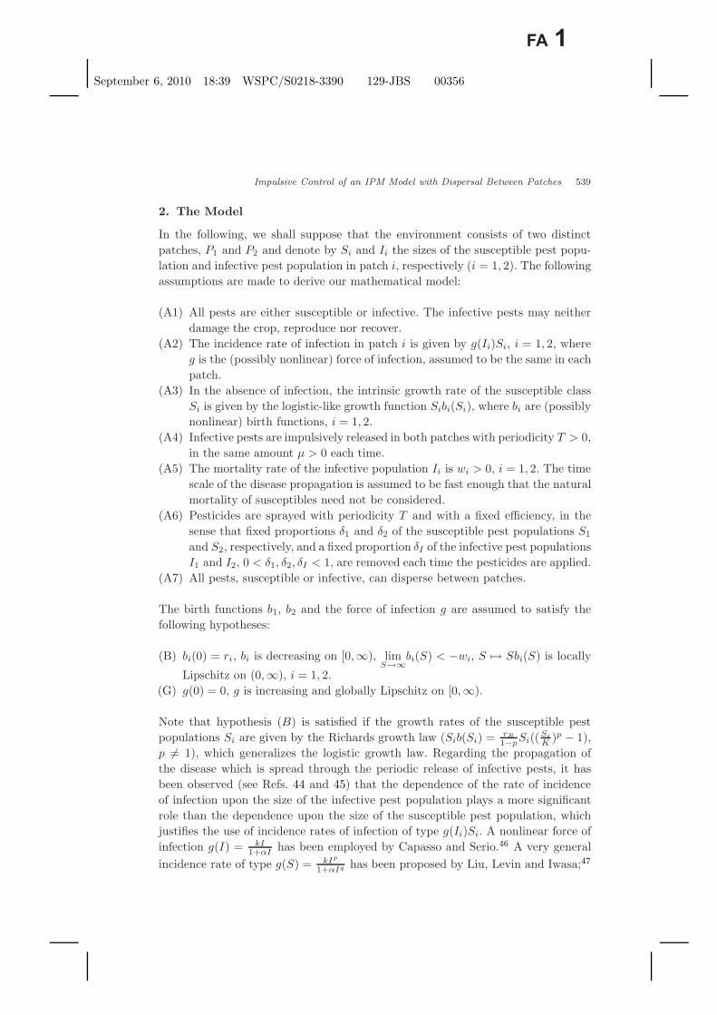
554 Georgescu, Dimitriu & Sinclair
≤ max
(ln(1 − δ) + r1T −
∫ T
0
g(I∗(s))ds, ln(1 − δ) + r2T −∫ T
0
g(I∗(s))ds
)
≤ 0,
i.e., neither the dispersion of susceptible pests nor the dispersion of infective pestshave the potential to destabilize the system.
(b) Both patches are unstable without dispersal, i.e.,
ln(1 − δ) + r1T −∫ T
0
g(I∗(s))ds > 0, ln(1 − δ) + r2T −∫ T
0
g(I∗(s))ds > 0.
Then
E(r1, r2, d12, d21, w, w, a, T )
≥(
ln(1 − δ) + r1T −∫ T
0
g(I∗(s))ds
)+
(ln(1 − δ) + r2T −
∫ T
0
g(I∗(s))ds
)
−|r1T − r2T |
≥ min
(ln(1 − δ) + r1T −
∫ T
0
g(I∗(s))ds, ln(1 − δ) + r2T −∫ T
0
g(I∗(s))ds
)
≥ 0,
i.e., if both patches are unstable in isolation, then E∗ is unstable.(c) One patch is stable and the other is unstable without dispersal. Suppose
that the first patch is stable and the second is unstable, i.e., ln(1 − δ) + r1T −∫ T
0 g(I∗(s))ds ≤ 0, ln(1 − δ) + r2T − ∫ T
0 g(I∗(s))ds > 0.If one of d12 and d21 is zero, then
E(r1, r2, d12, d21, w, w, a, T )
= 2 max
(ln(1 − δ) + r1T −
∫ T
0
g(I∗(s))ds, ln(1 − δ) + r2T −∫ T
0
g(I∗(s))ds
).
Consequently, if the dispersal rate of susceptible pests from the unstable patch tothe stable patch is large enough and the dispersal rate of susceptible pests fromthe stable patch to the unstable patch is 0, then E∗ is stable, i.e., the dispersal ofsusceptible pests from the unstable patch to the stable patch has the potential tostabilize the system. Also, if the dispersal rate of susceptible pests from the unstablepatch to the stable patch is 0, then E∗ is unstable, i.e., the dispersal of infectivepests cannot stabilize the system.

September 6, 2010 18:39 WSPC/S0218-3390 129-JBS 00356
Impulsive Control of an IPM Model with Dispersal Between Patches 555
If d12 = d21 = d, then
E(r1, r2, d, d, w, w, g, T )
=
(ln(1 − δ) + r1T −
∫ T
0
g(I∗(s))ds
)+
(ln(1 − δ) + r2T −
∫ T
0
g(I∗(s))ds
)
+(r1 − r2)2T 2√
(r1 − r2)2T 2 + 4d2T 2 + 2dT
and consequently
limd→∞
E(r1, r2, d, d, w, w, g, T )
=
(ln(1 − δ) + r1T −
∫ T
0
g(I∗(s))ds
)+
(ln(1 − δ) + r2T −
∫ T
0
g(I∗(s))ds
),
i.e., large equal dispersal rates of susceptible pests might stabilize the system pro-vided that,(
ln(1 − δ) + r1T −∫ T
0
g(I∗(s))ds
)+
(ln(1 − δ) + r2T −
∫ T
0
g(I∗(s))ds
)< 0,
or fail to stabilize it provided that the opposite inequality holds.
6. Numerical Simulations
Here, all units will be arbitrary.To illustrate our mathematical findings, we proceed to further investigate the
dynamics of the system (2.1) by using numerical simulations. To discuss the influ-ence of dispersal upon the stability of the susceptible pest-eradication periodic solu-tion E∗, let us first choose g(Ii) = kIi
1+αIiand Sib(Si) = riSi(1 − Si
K )2 for i = 1, 2,T = 1 and l = 0.5. We let d12 vary over the interval [0, 1], with 20 division points.The solutions of the impulsively perturbed system (2.1) are integrated over 10 peri-ods, with 110 time steps in each interval [0, lT ] and [lT, T ], using a fourth-orderRunge-Kutta method, the variation of Si and Ii, i = 1, 2 with respect to t and d12
being illustrated in what follows by means of three-dimensional plots. On the d12
and t axes, the numbers refer to the indices of the division points, rather than toabsolute values. Also, by a stable or unstable patch, respectively, we mean a patchin which, if considered in isolation, the corresponding susceptible pest-eradicationperiodic (0, I∗) for that patch is stable or unstable, respectively.
For d21 = 0.01, D12 = 0.8, D21 = 0.7, δ1 = 0.2, δ2 = 0.4, δI = 0.5, w1 = 0.1,w2 = 0.3, µ = 0.03, r1 = 0.99, r2 = 0.01, k = 1, K = 8, it is seen that the firstpatch is unstable, the second patch is stable and E∗ changes its stability for d12 in[0, 1], going from unstable to stable at d12 = 0.75. The behavior of the trajectory

September 6, 2010 18:39 WSPC/S0218-3390 129-JBS 00356
556 Georgescu, Dimitriu & Sinclair
Fig. 1. g(Ii) = kIi1+αIi
and Sib(Si) = riSi(1 − SiK
)2 for i = 1, 2, T = 1, l = 0.5, d21 = 0.01,
D12 = 0.8, D21 = 0.7, δ1 = 0.2, δ2 = 0.4, δI = 0.5, w1 = 0.1, w2 = 0.3, µ = 0.03, r1 = 0.99,r2 = 0.01, k = 1, K = 8. An increase in the dispersal of susceptible pests from an unstable patchto a stable patch has the potential to contribute to the success of the pest control strategy.
starting with S1(0) = 0.5, S2(0) = 0.8, I1(0) = 0.025, I2(0) = 0.04 is depicted inFig. 1. Since the dispersal of the susceptible pests from the second patch (the stableone) to the first patch (the unstable one) is weak, an increase in the dispersal ofsusceptible pests from the unstable patch to the stable patch has the potential tostabilize E∗ and therefore to contribute to the success of the pest control strategy.Note that the the gain of stability for E∗ occurs with an outburst in the size of thesusceptible pest class in the stable patch.
For d21 = 0.95, D12 = 0.85, D21 = 0.7, δ1 = 0.4, δ2 = 0.1, δI = 0.5, w1 = 0.1,w2 = 0.3, µ = 0.03, r1 = 0.95, r2 = 0.9, k = 1, K = 8, it is seen that both patchesare unstable and E∗ is unstable for d12 in [0, 1]. Also, the value of the instability-causing eigenvalue µ1 is increasing with d12. The behavior of the trajectory startingwith S1(0) = 0.5, S2(0) = 0.8, I1(0) = 0.025, I2(0) = 0.04 is depicted in Fig. 2. It isthen seen that the sizes of the susceptible pest populations in both patches increasenoticeably with the time, i.e., the dispersal of susceptible pest individuals from thefirst patch to the second patch has a negative impact upon the success of the pestcontrol strategy, fact with can be attributed to the increase in the value of µ1.
For d21 = 0.25, D12 = 0.9, D21 = 0.8, δ1 = 0.25, δ2 = 0.2, δI = 0.9, w1 = 0.1,w2 = 0.3, µ = 0.03, r1 = 0.25, r2 = 0.5, k = 2, K = 8, it is seen that the first patchis stable, the second patch is unstable and E∗ changes its stability for d12 in [0, 1],going from stable to unstable at d12 = 0.1. The behavior of the trajectory startingwith S1(0) = 0.5, S2(0) = 0.8, I1(0) = 0.025, I2(0) = 0.04 is depicted in Fig. 3,

September 6, 2010 18:39 WSPC/S0218-3390 129-JBS 00356
Impulsive Control of an IPM Model with Dispersal Between Patches 557
Fig. 2. g(Ii) = kIi1+αIi
and Sib(Si) = riSi(1 − SiK
)2 for i = 1, 2, T = 1, l = 0.5, d21 = 0.95,
D12 = 0.85, D21 = 0.7, δ1 = 0.4, δ2 = 0.1, δI = 0.5, w1 = 0.1, w2 = 0.3, µ = 0.03, r1 = 0.95,r2 = 0.9, k = 1, K = 8. The dispersal of susceptible pest individuals from patch P1 to patch P2
has a negative impact upon the success of the pest control strategy.
Fig. 3. g(Ii) = kIi1+αIi
and Sib(Si) = riSi(1 − SiK
)2 for i = 1, 2, T = 1, l = 0.5, d21 = 0.25,
D12 = 0.9, D21 = 0.8, δ1 = 0.25, δ2 = 0.2, δI = 0.9, w1 = 0.1, w2 = 0.3, µ = 0.03, r1 = 0.25,r2 = 0.5, k = 2, K = 8. An increase in the dispersal of susceptible pests from a stable patch toan unstable patch has the potential to destabilize the two-patch system.
where one sees that an increase in the dispersal of susceptible pests from the stablepatch to the unstable patch has the potential to destabilize E∗.
In an attempt to understand the nature of the bifurcation of solutions ofthe single-patch model system (2.2) described by Theorem 2.1, we performed a

September 6, 2010 18:39 WSPC/S0218-3390 129-JBS 00356
558 Georgescu, Dimitriu & Sinclair
large number of simulations using g(I) = 200 I/(40 + I) and b(S) = r − S/1000,T = 5, l = 0.5, δ1 = 0.8 δI/0.99, w = 10, µ = 0.03, r = 3, a choice made tohave some qualitative similarity to the case of the diamondback moth (high mor-tality rates for a highly contagious infection, high fecundity for the pest). Notethat the period of release of infective pests and of insecticide spraying (T ) is keptconstant. This reflects the fact that climate or life-cycle rhythms, as well as economicconsiderations, do not allow for complete freedom in the choice of this period inthe field. It would not make sense to spray pesticides every five minutes, for exam-ple. The susceptible pest-eradication periodic solution was first allowed to establishitself from initial conditions S(0) = 0 and I(0) = µ, and then perturbed at t = 400T
by adding a fixed number of susceptible pests (setting S(400T ) = 0.0001 in arbi-trary units). The solutions were then followed for another 1000T . Convergencewas checked using the highly conservative approach of comparing the values ofS(1400T ) and I(1400T ) computed using two different step sizes, differing by a fac-tor of two. If the absolute difference was less than a specified tolerance (0.000001),the simulation was considered to have converged, otherwise the number of stepswas increased until reaching a fixed limit. Each colored circle in Fig. 4 is the resultof a simulation which passed this convergence check. From these data sets, valuesat times nT + (after addition of infective pests according to ∆I(nT ) = µ) were
Fig. 4. An illustration of Theorem 2.1 using g(I) = 200 I/(40+I) and b(S) = r−S/1000, T = 5,l = 0.5, δ1 = 0.8 δI/0.99, w = 10, µ = 0.03, r = 3. Each point corresponds to one simulation runwith initial conditions S(0) = 0 and I(0) = µ, perturbed at t = 400 T by assigning S(400 T ) =0.0001. The green points indicate stability of the susceptible pest-eradication periodic solution.The black curve is the limit case defined by (2.7). The remaining points are coloured accordingto the periods of the corresponding solutions. White regions indicate failure of convergence of thenumerical method, presumably due to the solutions being chaotic.

September 6, 2010 18:39 WSPC/S0218-3390 129-JBS 00356
Impulsive Control of an IPM Model with Dispersal Between Patches 559
recorded. The final 41 such SI pairs (i.e. S(1360T +), S(1361T +), . . . , S(1400T +)and I(1360T +), I(1361T +), . . . , I(1400T +)) were then analysed for periodicity.According to the period detected, a color was chosen for the corresponding col-ored circle. What one sees is that the susceptible pest-eradication periodic solu-tion is indeed globally asymptotically stable (the green region of Fig. 4) if (2.5) issatisfied, confirming Theorem 2.1 (this is a test of the dedicated numerical softwarewe wrote). Once the limit case (2.7) is passed, we see the predicted bifurcation to astable positive period solution, confirming Theorem 2.2. What the theorems cannotexplain is the remaining structure of the region of instability. Numerically, it seemsthat period-doubling bifurcations leading to chaos are characteristic of this regime.From a biological point of view, what is interesting to note is that increasing thenumber of infective pests released (µ) will, if all other parameters are fixed to thevalues given above, always lead to control. On the other hand, simply increasingthe efficiency of the periodic pesticide spraying (increasing δ1 and δI , perhaps bysimply spraying more pesticide each time) does not typically lead to control.
In a large-scale numerical study, we used the dedicated software written forthe bifurcation study above to try to find parameter sets for which the individ-ual patches would be stable (S1(700T +) + S2(700T +) < 0.00003), but the two-patch system not. One sample parameter set found by this automated search wasdefined by δ1 = 18/25, δ2 = 18/25, δI = 891/1000, µ = 45.0, r1 = 2.781782,r2 = 6.245837, d12 = 0.077159, d21 = 0.306883, D12 = D21 = 0.1, w1 = 10.0,w2 = 4.951027, T = 5, l = 1/2, g(I) = I/(30 + I/1000), b1(S) = r1 − S/1000and b2(S) = r2 −S/1000. Note that this parameter set does not satisfy the relationbetween death rates and dispersal rates of pests (4.1) we have otherwise enforced fortechnical reasons. The dispersal rates of susceptibles are asymmetric. Such asymme-try could occur in the wild as the result of prevailing winds or altitude gradients and
Fig. 5. Instability of the susceptible pest-eradication periodic solution for the two-patch model,in a case in which each patch is stable in isolation. The loss of control is due to dispersion of pests.

September 6, 2010 18:39 WSPC/S0218-3390 129-JBS 00356
560 Georgescu, Dimitriu & Sinclair
directed water flow, for example. Since the parameter set was found by a numericalsimulation performed to hardware precision only (C double precision, correspond-ing to about 17 significant decimal digits), we also ran high-precision simulationsusing Maple74 computing with 400 decimal digit software floating-point numbersand a seventh-eighth order Runge-Kutta method. These high-precision calculationsstrongly support the initial calculations, leading us to believe that this parameterset does indeed represent a case in which dispersal between otherwise stable patchescan lead to a loss of control for the two-patch system (see Fig. 5). The two-patchsolution, once control is lost, appears to be chaotic.
7. Concluding Remarks
The focus of this paper is on investigating the behavior of a two-patch integratedpest management model which is subject to a biological control, consisting of theperiodic release of infective pests and to a chemical control, consisting of pesticidespraying, which are applied in a periodic fashion, with the same periodicity, butnot simultaneously. An abstract, unspecified force of infection, which is possiblynonlinear, is used to describe the spread of the disease which is propagated throughthe release of infective pests, assuming that both susceptible and infective pests cantravel between patches.
Since it is assumed that the infective pests neither damage crops nor reproduce,a measure for the success of the impulsive control strategy is represented by thestability properties of the susceptible pest-eradication periodic solution, which wediscussed using Floquet theory for periodic and impulsive systems of ordinary dif-ferential equations. In order for our approach to be consistent, a relation betweenthe death rates and the dispersal rates of infective pests has been assumed to hold.Note that, although it has been observed that the case in which infective pestscan reproduce with totally successful vertical transmission (i.e., any offspring of aninfective pest is an infective pest) can be reformulated to fit our framework, thecase of a imperfect vertical transmission (the offspring of infective pests can be bothsusceptible pests or infective pests) is not treatable using our approach.
The local stability of the susceptible pest-eradication periodic solution isobtained in terms of a condition which is significantly more complicated than itssingle-patch counterpart in Georgescu and Morosanu.38 This gives formal supportto the intuitive notion that the patch structure induces a nontrivial layer of com-plexity which is worth investigating.
A comparison with the corresponding results in Ref. 39 also reveals the fact thatthe dispersal of infective pests bears, in some sense, a more prominent role than thedispersal of susceptible pests. Supposing that only the susceptible pests are able todisperse between patches, it has been seen39 that the stability or instability of bothpatches in isolation is transmitted to the system at large regardless of the values ofthe dispersal rates, in sense that if both patches are stable or unstable in isolation,then the same can be said about the two-patch system. Note that, these findings

September 6, 2010 18:39 WSPC/S0218-3390 129-JBS 00356
Impulsive Control of an IPM Model with Dispersal Between Patches 561
agree with those of Takeuchi,32 who observed that, considering a patchy systemoccupied by a single species, if the species is able to survive at a globally stableequilibrium point when patches are isolated, it will continue to do so at a differentequilibrium in the presence of dispersal. However, it has been observed in our settingthat the dispersal of infective pests has the potential to destabilize an otherwisestable system, although it cannot do so, given certain technical assumptions, if thedeath rates of infective pests are the same in each patch. Also, if both patches areunstable in isolation, then the system at large will remain unstable regardless ofthe values of the dispersal rates of infective pests.
In a system with one stable and one unstable patch, it has been seen numericallythat an increase in the dispersal rate of the susceptible pest individuals from theunstable patch to the stable patch has the potential to stabilize the susceptiblepest-eradication periodic solution E∗ and to contribute to the success of the pestcontrol strategy, while an increase in the dispersal rate from the stable patch tothe unstable patch has the potential to destabilize E∗ and to be detrimental to thesuccess of the pest control strategy. Also, in a system with two unstable patches,an increase in the dispersal rate of susceptible pest individuals from one patch toanother can have a significant negative impact upon the success of the pest controlstrategy.
Numerical experiments have revealed complex bifurcation structure in theunstable regime of a single patch, and show that a simple increase in the amountof pesticide applied does not guarantee control of a pest. In a system with twopatches, both stable in the absence of dispersion, it has been seen that loss of con-trol in both patches can occur due to dispersal of pests. This was demonstrated inour model both analytically, in the case of equal efficiency of chemical control inboth patches, and also in a numerical simulation involving asymmetric dispersionbetween patches.
Acknowledgments
The work of P. Georgescu and G. Dimitriu was supported by by CNCSIS —UEFISCSU (Romania) project number PN II — IDEI 342/2008, contractno. 447/2009: “Nonlinear evolution equations — theoretical aspects and applica-tions to life and environmental sciences”.
References
1. Alavanja MC, Hoppin JA, Kamel F, Health effects of chronic pesticide exposure:cancer and neurotoxicity, Annu Rev Public Health 25:155–1997, 2004.
2. Kamel F, Hoppin JA, Association of pesticide exposure with neurologic dysfunctionand disease, Environ Health Perspect 112:950–958, 2004.
3. Richter ED, Acute human poisonings, Encyclopedia of Pest Management, Pimentel D(ed.), Dekker, New York, pp. 3–6, 2002.
4. Pimentel D, Environmental and economic costs of the application of pesticidesprimarily in the United States, Environ Dev Sustain 7:229–252, 2005.

September 6, 2010 18:39 WSPC/S0218-3390 129-JBS 00356
562 Georgescu, Dimitriu & Sinclair
5. Eskenazi B, Chevrier J, Rosas LG, Anderson HA, Bornman MS, Bouwman H, ChenA, Cohn BA, de Jager C, Henshel DS, Leipzig F, Leipzig JS, Lorenz EC, SnedekerSM, Stapleton D, The Pine River statement: human health consequences of DDT use,Environ Health Perspect 117:1359–1367, 2009.
6. Talekar NS, Shelton AM, Biology, Ecology, and management of the diamondbackmoth, Annu Rev Entomol 38:275–301, 1993.
7. Kogan M, Integrated pest management: historical perspectives and contemporarydevelopments, Annu Rev Entomol 43:243–270, 1998.
8. Smith RF, van den Bosch R, Integrated control, in Pest Control: Biological, Physicaland Selected Chemical Methods, Wendell W, Kilglore WW, Doutt RL (eds.), AcademicPress, New York, pp. 295–340, 1967.
9. De Maagd RA, Bravo A, Crickmore N, How Bacillus thuringiensis has evolved specifictoxins to colonize the insect world, TIG 17:193–199, 2001.
10. Raymond B, Wyres KL, Sheppard SK, Ellis RJ, Bonsall MB, Environmental factorsdetermining the epidemiology and population genetic structure of the Bacillus cereusgroup in the field, PloS Pathogens 6:e1000905, 2010.
11. DeBach P, Rosen D, Biological Control by Natural Enemies, Cambridge UniversityPress, 1991.
12. Nagai K, Yano E, Predation by Orius sauteri (Poppius) (Heteroptera: Anthocoridae)on Thrips palmi Karny (Thysanoptera: Thripidae). Functional response and selectivepredation, Appl Entomol Zool 35:565–574, 2000.
13. Port CM, Scopes NEA, Biological control by predatory mites (Phytoseiulus persimilisAthias-Henriot) of red spider mite (Tetranychus urticae Koch) infesting strawberriesgrown in walk-in plastic tunnels, Plant Pathology 30:95–99, 1981.
14. Grzywacz D, Parnell M, Kibata G, Oduor G, Ogutu W, Miano D, Winstanley D,The development of endemic baculoviruses of Plutella xylostella (diamondback moth,DBM) for control of DBM in East Africa, in The Management of DiamondbackMoth and Other Cruciferous Pests, Proceedings of the Fourth International Work-shop on Diamondback Moth, Endersby N, Ridland P (eds.), Melbourne University,pp. 179–183, 2001.
15. Brudea V, Modul de actiune al insecticidelor si al preparatelor biologice ın manage-mentul integrat al daunatorilor (Romanian), Bucovina Forestiera 1–2:93–100, 2004.
16. Rabb RL, Stinner RE, van den Bosch R, Conservation and augmentation of naturalenemies, Theory and Practice of Biological Control, Huffaker CB, Messenger PS (eds.),Academic Press, New York, pp. 233–254, 1976.
17. O’Neil R, Yaninek S, Landis S, Orr D, Biological control and integrated pest man-agement, Integrated Pest Management in the Global Arena, Maredia KM, Dakouo D,Mota-Sanchez D (eds.), Cabi Publishing, Wallingford, pp. 19–30, 2003.
18. Bainov D, Simeonov P, Impulsive Differential Equations: Periodic Solutions andApplications, Longman, John Wiley, New York, NY, 1993.
19. Haddad WM, Chellaboina V, Nersesov SG, Impulsive and Hybrid Dynamical Systems:Stability, Dissipativity and Control, Princeton University Press, Princeton and Oxford,2006.
20. Yang T, Impulsive Control Theory, Lecture Notes in Control and Information Sciences272, Springer, Berlin, 2001.
21. Mailleret L, Grognard F, Global stability and optimisation of a general impulsivebiological control model, Research Report, INRIA no. 6637, 2008.
22. Zhang H, Chen L, Georgescu P, Impulsive control strategies for pest management,J Biol Syst 15:235–260, 2007.
23. Tang S, Cheke R, State-dependent impulsive models of integrated pest management(IPM) strategies and their dynamic consequences, J Math Biol 50:257–292, 2005.

September 6, 2010 18:39 WSPC/S0218-3390 129-JBS 00356
Impulsive Control of an IPM Model with Dispersal Between Patches 563
24. Tang S, Tang G, Cheke R, Optimum timing for integrated pest management:modelling rates of pesticide application and natural enemy releases, J Theor Biol264:623–638, 2010.
25. Apreutesei N, Necessary optimality conditions for a Lotka-Volterra three species sys-tem, Math Modelling Nat Phenomena 1:123–135, 2006.
26. Apreutesei N, Dimitriu G, Optimal control for Lotka-Volterra systems with a hunterpopulation, Lecture Notes in Computer Science 4818, Springer Verlag, Berlin, 2008,pp. 277–284.
27. Begon M, Townsend CR, Harper JL, Ecology: From Individuals to Ecosystems,Blackwell Publishing, Oxford, U.K., 2006.
28. Wu J, Modelling dynamics of patchy landscapes: linking metapopulation theory, land-scape theory and conservation biology, Wealth, Health and Faith-Sustainability Studyin China, Wang R, Zhao J, Ouyang Z, Niu T (eds.), China Environmental SciencePress, Beijing, pp. 97–116, 1995.
29. Hauzy C, Hulot FD, Gins A, Loreau M, Intra- and interspecific density-dependentdispersal in an aquatic prey-predator system, J Anim Ecol 76:552–558, 2007.
30. Takeuchi Y, Cui J, Miyazaki R, Saito Y, Permanence of delayed population modelwith dispersal loss, Math Biosci 201:143–156, 2006.
31. Kuang Y, Takeuchi Y, Predator-prey dynamics in models of prey dispersal in two-patch environments, Math Biosci 120:77–98, 1994.
32. Takeuchi Y, Cooperative system theory and global stability of diffusion models, ActaAppl Math 14:49–57, 1989.
33. Hsieh YH, van den Driessche P, Wang L, Impact of travel between patches for spatialspread of disease, Bull Math Biol 69:1355–1375, 2007.
34. Takeuchi Y, Wang W, Saito Y, Global stability of population models with patchstructure, Nonlinear Anal Real World Appl 7:235–247, 2006.
35. Goldwyn E, Hastings A, When can dispersal synchronize populations? Theor PopBiol 73:395–402, 2008.
36. Briggs C, Hoopes M, Stabilizing effects in spatial parasitoid-host and predator-preymodels: a review, Theor Pop Biol 65:299–315, 2004.
37. El Abdllaoui A, Auger P, Kooi B, Bravo de la Parra R, Mchich R, Effects of density-dependent migrations on stability of a two-patch predator-prey model, Math Biosci210:335–354, 2007.
38. Georgescu P, Morosanu G, Pest regulation by means of impulsive controls, Appl MathComput 190:790–803, 2007.
39. Georgescu P, Zhang H, The impulsive control of a two-patch integrated pest manage-ment model, Proceedings of 6-th Edition of International Conference on Theory andApplications of Mathematics and Informatics, Breaz D, Breaz N, Wainberg D (eds.),Iasi, Romania, Acta Univ. Apulensis, Math. Inform. (Special Issue), Aeternitas Pub-lishing House, 2009, pp. 297–320.
40. May RM, Biological populations with nonoverlapping generations: stable points, sta-ble cycles, and chaos, Science 186:645–647, 1974.
41. Pascual M, Diffusion-induced chaos in a spatial predator-prey system, Proc R SocLond B 251:1–7, 1993.
42. Koelle K, Vandermeer J, Dispersal-induced desynchronization: from metapopulationsto metacommunities, Ecol Lett 8:167–175, 2005.
43. Yang J, Tang S, Effects of population dispersal and impulsive control tactics on pestmanagement, Nonlinear Anal Hybrid Syst 3:487–500, 2009.
44. Liu WM, Hethcote HW, Levin SA, Dynamical behavior of epidemiological modelswith nonlinear incidence rates, J Math Biol 25:359–380, 1987.

September 6, 2010 18:39 WSPC/S0218-3390 129-JBS 00356
564 Georgescu, Dimitriu & Sinclair
45. Korobeinikov A, Maini PK, Non-linear incidence and stability of infectious diseasemodels, Math Med Biol 22:113–128, 2005.
46. Capasso V, Serio G, A generalization of Kermack-McKendrick deterministic epidemicmodel, Math Biosci 42:43–61, 1978.
47. Liu WM, Levin SA, Iwasa Y, Influence of nonlinear incidence rates on the behaviorof SIRS epidemiological models, J Math Biol 23:187–204, 1986.
48. Hethcote HW, van den Driessche P, Some epidemiological models with nonlinearincidence, J Math Biol 29:271–287, 1991.
49. Ruan S, Wang W, Dynamical behavior of an epidemic model with a nonlinear inci-dence rate, J Differential Equations 188:135–163, 2003.
50. Xiao D, Ruan S, Global analysis of an epidemic model with nonmonotone incidencerate, Math Biosci 208:419–429, 2007.
51. Contamine D, Gaumer S, Sigma Rhabdoviruses, Encyclopedia of Virology, 3rd. edn.,Volume 4, Mahy BWJ, Van Regenmortel MHV (eds.), Academic Press, Amsterdam,2008, pp. 576–581.
52. Andreadis TG, Evolutionary strategies and adaptations for survival betweenmosquito-parasitic microsporidia and their intermediate copepod hosts: a comparativeexamination of Amblyospora connecticus and Hyalinocysta chapmani (Microsporidia:Amblyosporidae), Folia Parasitologica 52:23–35, 2005.
53. Dodd IB, Shearwin KE, Egan JB, Revisited gene regulation in bacteriophage λ, CurrOpin Genet Dev 15:145–152, 2005.
54. Chen Y, Evans J, Feldlaufer M, Horizontal and vertical transmission of viruses in thehoney bee, Apis mellifera, J Invertebr Pathol 92:152–159, 2006.
55. Bouchon D, Rigaud T, Juchault P, Evidence for widespread Wolbachia infectionin isopod crustaceans: molecular identification and host feminization, Proc Biol Sci265:1081–1090, 1998.
56. Cory JS, Myers JH, The ecology and evolution of insect baculoviruses, Annu Rev EcolEvol Systemat 34:239–272, 2003.
57. Nordin GL, Brown GC, Jackson DM, Vertical transmission of two baculovirusesinfectious to the tobacco budworm, Heliothis virescens (F.) (Lepidoptera: Noctuidae)using an autodissemination technique, J Kansas Entomol Soc 63:393–398,1990.
58. Stewart AD, Logsdon JM, Kelley SE, An empirical study of the evolution of virulenceunder both horizontal and vertical transmission, Evolution 59:730–739, 2005.
59. Lambrechts L, Scott TW, Mode of transmission and the evolution of arbovirus viru-lence in mosquito vectors, Proc R Soc B 276:1369–1378, 2009.
60. Dunn AM, Smith JE, Microsporidian life cycles and diversity: the relationship betweenvirulence and transmission, Microb Infect 3:381–388, 2001.
61. Talekar NS, Biological control of diamondback moth in Taiwan — a review, PlantProt Bull 38:167–189, 1996.
62. Rondon SI, The Potato Tuberworm: a literature review of its biology, ecology, andcontrol, Am J Pot Res 87:149–166, 2010.
63. Hilton S, Baculoviruses: molecular biology of ganuloviruses, Encyclopedia of Virology,3rd. edn., Volume 1, Mahy BWJ, Van Regenmortel MHV (eds.), Academic Press,Amsterdam, 2008, pp. 211–219.
64. Dezianian A, Sajap AS, Lau WH, Omar D, Kadir HA, Mohamed R, Yusoh MRM,Morphological characteristics of P. xylostella granulovirus and effects on its larvalhost diamondback moth Plutella xylostella L. (Lepidoptera, Plutellidae), Am J AgricBio Sci 5:43–49, 2010.

September 6, 2010 18:39 WSPC/S0218-3390 129-JBS 00356
Impulsive Control of an IPM Model with Dispersal Between Patches 565
65. Arthurs SP, Lacey LA, De La Rosa F, Evaluation of a Granulovirus (PoGV) and Bacil-lus thuringiensis subsp. kurstaki for control of the potato tuberworm (Lepidoptera:Gelechiidae) in stored tubers, J Econ Entomol 101:1540–1546, 2008.
66. Volkman LE, Baculoviruses: Pathogenesis, in Encyclopedia of Virology, 3rd. edn.,Volume 1, Mahy BWJ, Van Regenmortel MHV (eds.), Academic Press, Amsterdam,2008, pp. 265–272.
67. Nakai M, Goto C, Shiotsuki T, Kunimi Y, Granulovirus prevents pupation and retardsdevelopment of Adoxophyes honmai larvae, Physiol Entomol 27:157–164, 2002.
68. Hoy MA, Myths, models and mitigation of resistance to pesticides, Phil Trans R SocLond B 353:1787–1795, 1998.
69. Lee Y, Fuxa JR, Transport of wild-type and recombinant nucleopolyhedroviruses byscavenging and predatory arthropods, Microb Ecol 39:301–313, 2000.
70. Georgescu P, Zhang H, Chen L, Bifurcation of nontrivial periodic solutions for animpulsively controlled pest management model, Appl Math Comput 202:675–687,2008.
71. Bacaer N, Ouifki R, Growth rate and basic reproduction number for population mod-els with a simple periodic factor, Math Biosci 210: 647–658, 2007.
72. Bacaer N, Periodic matrix population models: growth rate, basic reproduction numberand entropy, Bull Math Biol 71: 1781–1792, 2009.
73. Wang W, Zhao XQ, Threshold dynamics for compartmental epidemic models in peri-odic environments, J Dyn Diff Eq 20:699–717, 2008.
74. Monagan MB, Geddes KO, Heal KM, Labahn G, Vorkoetter SM, McCarron J,DeMarco P, Maple 10 Programming Guide, Maplesoft, Waterloo ON, Canada, 2005.
Appendix: The Exponential Representation Formula
To write the fundamental matrix Φ(t) of (2.1) as a matrix exponential, we firststate several considerations regarding the exponential representation formula forthe solutions of a n-dimensional time-dependent homogeneous linear differentialsystem.
Let us consider the differential system with continuous coefficients
x′(t) = B(t)x(t), t ≥ 0. (A.1)
The fundamental matrix of (A.1) which satisfies Φ(0) = In can be expressed as aPeano-Baker series of the form,
Φ(t) = In +∫ t
0
B(s1)ds1 +∫ t
0
B(s1)∫ s1
0
B(s2)ds2ds1 (A.2)
+∫ t
0
B(s1)∫ s1
0
B(s2)∫ s2
0
B(s3)ds3ds2ds1 + · · · .
To compute a monodromy matrix, a closed form representation of Φ would besignificantly more useful. If B commutes with its integral, i.e.,
B(t)(∫ t
0
B(s)ds
)=(∫ t
0
B(s)ds
)B(t) for t ≥ 0, (A.3)

September 6, 2010 18:39 WSPC/S0218-3390 129-JBS 00356
566 Georgescu, Dimitriu & Sinclair
then the fundamental matrix Φ can be expressed as the exponential of a time-dependent matrix, in the form,
Φ(t) = exp(∫ t
0
B(s)ds
),
where, given N ∈ Mn(R), exp(N) is defined as,
exp(N) =∞∑
k=0
1k!
Nk.
Note that, in general, the fundamental matrix Φ given by (A.2) may be differentfrom exp(
∫ t
0 B(s)ds) if B does not satisfy (A.3). Also, it is easy to see that (A.3)holds if B(t) commutes with B(s) for all t, s ≥ 0, i.e.,
B(t)B(s) = B(s)B(t) for t, s ≥ 0. (A.6)
In this regard, note that the applicability of the results in Yang and Tang43 shouldbe somewhat restricted, as no commutation condition is verified therein.
Appendix B: The Proof of Lemma 4.1
Proof. Let C =(−(w1 + D12) D21
D12 −(w2 + D21)
)and let us also denote by (I∗1 , I∗2 )t the
desired periodic solution of (4.2). Obviously, one should have
(I∗1 (t)I∗2 (t)
)=
exp(tC)
(I∗1 (0+)
I∗2 (0+)
), t ∈ (0, lT ]
(1 − δI) exp(tC)
(I∗1 (0+)
I∗2 (0+)
), t ∈ (lT, T ].
By the T -periodicity requirement, it is seen that the initial data should satisfy
(1 − δI)eTC
(I∗1 (0+)I∗2 (0+)
)+(
µ
µ
)=(
I∗1 (0+)I∗2 (0+)
). (B.2)
Let
λ1,2 =−[(w1 + D12) + (w2 + D21)] ±
√[(w1 + D12) − (w2 + D21)]2 + 4D12D21
2be the (real) eigenvalues of C. Since
λ1 + λ2 = −(w1 + D12) − (w2 + D21) < 0
λ1 · λ2 = (w1 + D12)(w2 + D21) − D12D21 > 0,
it follows that λ1, λ2 < 0. Consequently, the eigenvalues of exp(TC) are eλ1T ,eλ2T ∈ (0, 1), which implies that I2 − (1 − δI) exp(TC) is invertible, and(
I∗1 (0+)I∗2 (0+)
)= (I2 − (1 − δI) exp(TC))−1
(µ
µ
).

September 6, 2010 18:39 WSPC/S0218-3390 129-JBS 00356
Impulsive Control of an IPM Model with Dispersal Between Patches 567
Now, it is seen that I∗1 − I∗2 verifies
(I∗1 − I∗2 )′(t) = −(w1 + 2D12)(I∗1 − I∗2 )(t), t �= (n + l − 1)T, t �= nT ;
∆(I∗1 − I∗2 )(t) = −δI(I∗1 − I∗2 )(t), t = (n + l − 1)T ;
∆(I∗1 − I∗2 )(t) = 0, t = nT,
which implies that limt→∞(I∗1 (t) − I∗2 (t)) = 0 and, since I∗1 , I∗2 are T -periodic, I∗1 ≡
I∗2 ≡ I∗. Now, I∗ verifies
I∗ = −w1 + w2
2I∗, t �= (n + l − 1)T, t �= nT ;
∆I∗ = −δII∗, t = (n + l − 1)T ;
∆I∗ = µ, t = nT
and the periodicity condition (B.2) translates as,
(1 − δI)e−w1+w2
2 T I∗(0+) + µ = I∗(0+),
which implies that
I∗(0+) =µ
1 − (1 − δI)e−w1+w2
2 T.
Consequently, I∗ is given by,
I∗(t) =
µ
1 − (1 − δI)e−w1+w2
2 Te−
w1+w22 (t−(n−1)T ), t ∈ ((n − 1)T, (n + l − 1)T ]
µ(1 − δI)
1 − (1 − δI)e−w1+w2
2 Te−
w1+w22 (t−(n−1)T ), t ∈ ((n + l − 1)T, nT ]
,
and the susceptible pest-eradication periodic solution E∗ of (2.1) is given by,
E∗ = (0, 0, I∗, I∗).
Now let (I1, I2)t be a solution of (4.2). As (I1 − I∗, I2 − I∗)t satisfies the system
(I1 − I∗
I2 − I∗
)′
(t) = C
(I1 − I∗
I2 − I∗
)(t), t �= (n + l − 1)T, t �= nT ;
∆
(I1 − I∗
I2 − I∗
)(t) = (1 − δI)
(I1 − I∗
I2 − I∗
)(t), t = (n + l − 1)T ;
∆
(I1 − I∗
I2 − I∗
)(t) = 0, t = nT
,

September 6, 2010 18:39 WSPC/S0218-3390 129-JBS 00356
568 Georgescu, Dimitriu & Sinclair
it is seen that,
(I1 − I∗
I2 − I∗
)(t) =
(1 − δI)n−1 exp (tC)
(I01 − I∗(0+)
I02 − I∗(0+)
), t ∈ ((n − 1)T, (n + l − 1)T ]
(1 − δI)n exp (tC)
(I01 − I∗(0+)
I02 − I∗(0+)
), t ∈ ((n + l − 1)T, nT ].
Since the eigenvalues of exp (TC) are eλ1T , eλ2T ∈ (0, 1) and exp ((t − (n − 1)T )C)is bounded for t ∈ ((n − 1)T, nT ], it is seen that,
limn→∞‖(1 − δI)n−1 exp ((n − 1)TC)‖ = 0
for any matrix norm ‖ · ‖, from which the conclusion follows.
Appendix C: The Proof of the Commutation Condition
It is seen that
A(t)(∫ t
0
A(s)ds
)=
a1(t)
∫ t
0 a1(s)ds + d12d21t d21
(ta1(t) +
∫ t
0 a2(s)ds)
d12
(ta2(t) +
∫ t
0a1(s)ds
)a2(t)
∫ t
0a2(s)ds + d12d21t
,
(∫ t
0
A(s)ds
)A(t) =
a1(t)
∫ t
0a1(s)ds + d12d21t d12
(ta2(t) +
∫ t
0a1(s)ds
)d21
(ta1(t) +
∫ t
0 a2(s)ds)
a2(t)∫ t
0 a2(s)ds + d12d21t
with
a1(t) = (r1 − d12) − g(I∗(t))
a2(t) = (r2 − d21) − g(I∗(t)).
Also,
ta2(t) +∫ t
0
a1(s)ds = t(r1 − d12 + r2 − d21) − tg(I∗(t)) −∫ t
0
g(I∗(s))ds
= ta1(t) +∫ t
0
a2(s)ds,
from which we deduce that
A(t)(∫ t
0
A(s)ds
)=(∫ t
0
A(s)ds
)A(t), ∀ t ≥ 0.
This commutation condition represents the motivation for using the same nonlinearforce of infection g and the same proportional loss of infective pests δI in each patchand also for using condition (4.1), meant to ensure that the limiting susceptible

September 6, 2010 18:39 WSPC/S0218-3390 129-JBS 00356
Impulsive Control of an IPM Model with Dispersal Between Patches 569
pest-eradication periodic solution has identical components in each patch. In thisregard, if different nonlinear forces of infection g1 and g2 were used in each patchand the susceptible pest-eradication periodic solution had distinct components I∗1and I∗2 for each patch, then the desired equality
t(g1(I∗1 (t)) − g2(I∗2 (t))) =∫ t
0
(g1(I∗1 (s)) − g2(I∗2 (s)))ds ∀ t ≥ 0
would not necessarily hold, as this would imply that t �→ g1(I∗1 (t)) − g2(I∗2 (t)) is aconstant function. Now, for g1 = g2 = g and I∗1 = I∗2 = I∗, it is seen from (4.2)that I∗ satisfies
(I∗)′(t) = (−w1 + D21 − D12)I∗(t) t �= (n + l − 1)T, t �= nT
(I∗)′(t) = (−w2 + D12 − D21)I∗(t),
from which we deduce that −w1 + D21 −D12 = −w2 + D12 −D21, i.e. (4.1) holds.


![Terminix integrated pest management [ipm] pest control indonesia](https://img.dokumen.tips/doc/110x75/556c5d50d8b42acc228b5069/terminix-integrated-pest-management-ipm-pest-control-indonesia.jpg)