IMPROVING STUDENTS’ UNDERSTANDING OF … · Electricity and magnetism are important ... multiple choice questions and essay ... 4.5.11 Invoking the dynamics of charges in an electrostatics

IMPROVING STUDENTS’ UNDERSTANDING OF ELECTRICITY AND MAGNETISM

by

Jing Li

B.S, University of Science and Technology of China, 2008

M.S., University of Pittsburgh, 2009

Submitted to the Graduate Faculty of

Department of Physics and Astronomy in partial fulfillment

of the requirements for the degree of

Doctor of Philosophy

University of Pittsburgh

2012

ii

UNIVERSITY OF PITTSBURGH

KENNETH P. DIETRICH SCHOOL OF ARTS AND SCIENCES

DEPARTMENT OF PHYSICS AND ASTRONOMY

This dissertation was presented

by

Jing Li

It was defended on

March 20th, 2012

and approved by

Dr. Rainer Johnsen, Professor Emeritus, Department of Physics and Astronomy

Dr. Russell Clark, Lecturer, Department of Physics and Astronomy

Dr. Arthur Kosowsky, Associate Professor, Department of Physics and Astronomy

Dr. Larry Shuman, Professor, Department of Industrial Engineering

Dissertation Advisor: Dr. Chandralekha Singh, Professor, Department of Physics

and Astronomy

iii

Copyright © by Jing Li

2012

iv

Electricity and magnetism are important topics in physics. Research shows that students have

many common difficulties in understanding concepts related to electricity and magnetism.

However, research to improve students’ understanding of electricity and magnetism is limited

compared to introductory mechanics. This thesis explores issues related to students’ common

difficulties in learning some topics in electricity and magnetism and how these difficulties can be

reduced by research-based learning tutorials. We investigated students’ difficulties in solving

problems involving light bulbs and equations involving circuit elements. We administered

multiple choice questions and essay questions to many classes and conducted individual

interviews with a subset of students. Based on these investigations, we provide suggestions to

improve learning. We also developed and evaluated five tutorials on Coulomb’s law, Gauss’s

law and the superposition principle to help students build a robust knowledge structure and firm

understanding of these concepts. Students’ performance on the corresponding pre- and post-tests

indicates that these tutorials effectively improved their understanding. We also designed a

Magnetism Conceptual Survey (MCS) that can help instructors probe students’ understanding of

magnetism concepts. The validity and reliability of this MCS is discussed. The performance of

students from different groups (e.g. female students vs. male students, calculus-based students

vs. algebra-based students) was compared. We also compare the MCS and the Conceptual

Survey of Electricity and Magnetism (CSEM) on common topics.

IMPROVING STUDENTS’ UNDERSTANDING OF ELECTRICITY AND

MAGNETISM

Jing Li, PhD

University of Pittsburgh, 2012

v

TABLE OF CONTENTS

PREFACE ............................................................................................................................... XVII

1.0 INTRODUCTION ........................................................................................................ 1

1.1 MOTIVATION .................................................................................................... 1

1.1.1 Traditionally taught E&M is challenging ..................................................... 1

1.1.2 Developing reasoning skills is important for student learning .................... 4

1.2 INFLUENCE FROM COGNITIVE SCIENCE ............................................... 5

1.2.1 Memory and cognitive load ............................................................................ 6

1.2.2 Alternative conceptions or Misconceptions ................................................... 7

1.2.3 Optimal mismatch and the zone of proximal development ......................... 9

1.2.4 Preparation for future learning.................................................................... 10

1.2.5 Guided inquiry ............................................................................................... 12

1.3 A STUDY OF STUDENTS’ UNDERSTANDING IN THE CONTEXT OF

E&M ............................................................................................................................. 14

1.3.1 Investigation of students’ difficulties with circuits involving light bulbs . 14

1.3.2 Student difficulties with equations involving circuit elements .................. 15

1.3.3 Coulomb’s law, superposition principle and Gauss’s law ......................... 16

1.3.4 Magnetism conceptual survey ...................................................................... 17

1.4 CHAPTER REFERENCES .............................................................................. 18

vi

2.0 STUDENTS’ CONCEPTUAL DIFFICULTIES WITH LIGHT BULBS

CONNECTED IN SERIES AND PARALLEL ........................................................................ 21

2.1 ABSTRACT ........................................................................................................ 21

2.2 INTRODUCTION ............................................................................................. 22

2.3 METHOD OF INVESTIGATION ................................................................... 26

2.4 RESULTS ........................................................................................................... 30

2.4.1 Light bulbs connected in parallel or series with resistance provided ....... 31

2.4.2 Light bulbs connected in parallel or series with standard power supply

provided ...................................................................................................................... 32

2.4.3 Comparison of the performance of introductory students with physics

graduate students ....................................................................................................... 34

2.5 DISCUSSION ..................................................................................................... 36

2.5.1 Students’ difficulties ...................................................................................... 36

2.5.2 Are these questions quantitative or conceptual? ........................................ 41

2.6 SUMMARY AND CONCLUSION .................................................................. 43

2.7 REFERENCES .................................................................................................. 44

3.0 STUDENT DIFFICULTIES WITH EQUATIONS INVOLVING CIRCUIT

ELEMENTS ................................................................................................................................ 45

3.1 ABSTRACT ........................................................................................................ 45

3.2 INTRODUCTION ............................................................................................. 46

3.3 METHODOLOGY ............................................................................................ 46

3.4 RESULTS ........................................................................................................... 49

3.5 DISCUSSION ..................................................................................................... 51

vii

3.6 SUMMARY AND CONCLUSION .................................................................. 55

3.7 REFERENCES .................................................................................................. 57

4.0 IMPROVING STUDENTS’ UNDERSTANDING OF ELECTROSTATICS I.

COULOMB’S LAW AND SUPERPOSITION PRINCIPLE ................................................. 58

4.1 ABSTRACT ........................................................................................................ 58

4.2 INTRODUCTION ............................................................................................. 58

4.3 OTHER INVESTIGATIONS RELATED TO ELECTRICITY AND

MAGNETISM ..................................................................................................................... 60

4.4 TUTORIAL DEVELOPMENT AND ADMINISTRATION ......................... 61

4.5 DISCUSSION OF STUDENTS’ DIFFICULTIES ......................................... 65

4.5.1 If distances from different charges add up to the same value at two points,

the electric field will be the same at those points ..................................................... 66

4.5.2 Only the nearest charge contributes to the electric field at a point .......... 72

4.5.3 Charges in a straight line that are blocked by other charges do not

contribute to the electric field.................................................................................... 72

4.5.4 Confusion between the electric field due to an individual charge and the

net electric field due to all charges ............................................................................ 73

4.5.5 Confusion between electric field, electric force and electric charge ......... 73

4.5.6 Electric field can only be found at points where there is a charge present ..

......................................................................................................................... 74

4.5.7 Assuming that a positive charge attracts all points around it so that the

electric field due to the charge points towards it ..................................................... 75

viii

4.5.8 Confusion about electric field line representation and interpretation of

electric field using it ................................................................................................... 76

4.5.9 Electric field cannot be zero at any point in a region if only positive

charges are present .................................................................................................... 79

4.5.10 Difficulty with the electric field due to an electric dipole at points on the

perpendicular bisector ............................................................................................... 80

4.5.11 Invoking the dynamics of charges in an electrostatics problem .............. 82

4.5.12 Confusion about symmetry of charge distribution vs. symmetry of the

object in which charges are distributed ................................................................... 83

4.5.13 Difficulties in generalizing from discrete to continuous charge

distribution ................................................................................................................. 84

4.6 PERFORMANCE OF TUTORIAL AND CONTROL GROUPS ................ 86

4.7 SUMMARY ........................................................................................................ 90

4.8 ACKNOWLEDGMENTS ................................................................................. 90

4.9 REFERENCES .................................................................................................. 90

5.0 IMPROVING STUDENTS’ UNDERSTANDING OF ELECTROSTATICS II.

SYMETRY AND GAUSS’S LAW ............................................................................................ 94

5.1 ABSTRACT ........................................................................................................ 94

5.2 INTRODUCTION ............................................................................................. 94

5.3 TUTORIAL TOPIC .......................................................................................... 97

5.4 DISCUSSION OF STUDENT DIFFICULTIES ............................................. 99

5.4.1 Difficulty with the principle of superposition ............................................. 99

ix

5.4.2 Measuring distances from the surface of a uniformly charged sphere or

cylinder ...................................................................................................................... 100

5.4.3 Magnitude of the net electric field is the sum of the magnitudes of the

components ............................................................................................................... 101

5.4.4 Confusion that a non-conductor completely shields the inside from the

electric field due to outside charges ........................................................................ 102

5.4.5 Difficulty realizing that electric flux can be calculated without knowing

electric field at each point on a closed surface ....................................................... 107

5.4.6 Ignoring the symmetry of the problem and assuming that the electric flux

is always EA ...................................................................................................... 108

5.4.7 Confusion about the underlying symmetry of a charge distribution ...... 110

5.4.8 Difficulty in determining how symmetric is symmetric enough to find the

electric field using Gauss’s law ............................................................................... 111

5.4.9 Difficulty in drawing a Gaussian surface to find the electric field at a

point due to a symmetric charge distribution ....................................................... 112

5.4.10 Confusing electric flux for a vector ........................................................... 117

5.4.11 Confusion between electric flux and electric field ................................... 117

5.4.12 Confusion between open and closed surfaces and Gauss’s law .............. 120

5.4.13 There must be a charge present at the point where the electric field is

desired ...................................................................................................................... 120

5.4.14 Assuming a point charge is present if the charge distribution in a region

is not given explicitly ................................................................................................ 121

5.4.15 Difficulty visualizing in three dimensions ................................................ 122

x

5.4.16 Student difficulty with basic mathematical tools ..................................... 123

5.4.17 Student difficulty with scientific language ............................................... 124

5.4.18 If A implies B then B must imply A or other convoluted reasoning ...... 127

5.5 PERFORMANCE OF TUTORIAL AND CONTROL GROUPS .............. 130

5.6 CONCLUSION ................................................................................................ 135

5.7 ACKNOWLEDGEMENTS ............................................................................ 135

5.8 REFERENCES ................................................................................................ 135

6.0 DEVELOPING A MAGNETISM CONCEPTUAL SURVEY ............................ 137

6.1 ABSTRACT ...................................................................................................... 137

6.2 INTRODUCTION ........................................................................................... 138

6.3 MAGNETISM CONCEPTUAL SURVEY DESIGN ................................... 139

6.4 MCS ADMINISTRATION ............................................................................. 141

6.5 DISCUSSION OF STUDENT DIFFICULTIES ........................................... 143

6.5.1 Magnetic force between bar magnets ........................................................ 148

6.5.2 Distinguishing between magnetic poles and charges ................................ 148

6.5.3 Magnetic field of a bar magnet ................................................................... 150

6.5.4 Directions of magnetic force, velocity and magnetic field ....................... 150

6.5.5 Work done by magnetic force..................................................................... 152

6.5.6 Movement doesn’t necessarily imply force ............................................... 153

6.5.7 Net force on a charged particle or a current carrying wire in a magnetic

field ....................................................................................................................... 154

6.5.8 Distinguishing between current carrying wires pointing into/out of the

page and static charges ............................................................................................ 157

xi

6.5.9 Magnetic field due to current loops ........................................................... 160

6.5.10 3D visualization and right hand rule ........................................................ 160

6.5.11 Performance of upper-level undergraduates ........................................... 161

6.5.12 Performance of graduate students ............................................................ 163

6.6 PERFORMANCE BY GENDER ................................................................... 164

6.7 ALGEBRA-BASED COURSES VS. CALCULUS-BASED COURSES .... 168

6.8 PERFORMANCE ON CSEM ........................................................................ 170

6.9 SUMMARY ...................................................................................................... 173

6.10 REFERENCES ................................................................................................ 173

7.0 CONCLUSION AND FUTURE CONSIDERATIONS ........................................ 175

7.1 INVESTIGATION OF STUDENTS’ DIFFICULTIES ............................... 175

7.2 COULOMB’S LAW, SUPERPOSITION PRINCIPLE AND GAUSS’S

LAW TUTORIALS .......................................................................................................... 176

7.3 MAGNETISM CONEPTUAL SURVEY ...................................................... 177

APPENDIX A ............................................................................................................................ 179

APPENDIX B ............................................................................................................................ 183

APPENDIX C ............................................................................................................................ 187

APPENDIX D ............................................................................................................................ 205

APPENDIX E ............................................................................................................................ 242

xii

LIST OF TABLES

Table 2.1. Introductory students’ responses to each free-response question with known

resistances ..................................................................................................................................... 31

Table 2.2. Introductory students’ responses to both free-response questions with known

resistances ..................................................................................................................................... 32

Table 2.3. Introductory students’ responses to each free-response question with known wattage

rating for a household power supply. ............................................................................................ 33

Table 2.4. Introductory students’ responses to both free-response questions with known wattage

rating for each bulb for a household power supply. ...................................................................... 33

Table 2.5. Graduate students’ responses to multiple-choice questions. ....................................... 36

Table 3.1. Distribution of introductory students’ responses to the multiple-choice questions. .... 50

Table 3.2.Distribution of introductory students’ responses to the free-response questions. ........ 50

Table 3.3. Distribution of physics graduate students’ responses to the multiple-choice questions.

....................................................................................................................................................... 51

Table 4.1 : Average percentage scores obtained on individual questions on the pre-/post-tests in

tutorial classes. .............................................................................................................................. 87

Table 4.2 : Average percentage scores obtained on individual questions on the pre-/post-tests in

non-tutorial class. .......................................................................................................................... 88

xiii

Table 4.3 : P values for the t-tests comparing performance of tutorial classes and non-tutorial

classes on the pre-/post-tests. ........................................................................................................ 88

Table 4.4 : Percentage average pre-/post-test scores (matched pairs) in tutorial classes for each of

the two tutorials (I-II), divided into three groups according to the pre-test performance. ........... 89

Table 4.5 : Percentage average pre-/post-test scores (matched pairs) in non-tutorial class related

to each of the two tutorials (I-II), divided into three groups according to the pre-test performance.

....................................................................................................................................................... 89

Table 5.1 : Average percentage scores obtained on individual questions on the pre-/post-tests for

tutorial classes ............................................................................................................................. 130

Table 5.2 : Average percentage scores obtained on individual questions on the pre-/post-tests for

the non-tutorial class. .................................................................................................................. 131

Table 5.3 : P value for t-tests comparing performance of tutorial classes and non-tutorial classes

on the pre-/post-tests. .................................................................................................................. 131

Table 5.4 : Percentage average pre-/post-test scores (matched pairs) in tutorial classes for each of

the three tutorials (III-V), divided into three groups according to the pre-test performance. ..... 132

Table 5.5 : Percentage average pre-/post-test scores (matched pairs) in non-tutorial class related

to each of the three tutorials (III-V), divided into three groups according to the pre-test

performance. ............................................................................................................................... 133

Table 5.6 : The average percentage of correct responses to each of the 25 questions on the

cumulative test (Singh 2006) for different student population. .................................................. 134

Table 6.1 : Concepts covered and the questions that addressed them in the test ........................ 145

Table 6.2 : Percentage of introductory algebra- based physics students who selected choices (a)-

(e) on Problems (1)-(30) on the test. ........................................................................................... 146

xiv

Table 6.3 : Percentage of introductory calculus- based physics students who selected choices (a)-

(e) on Problems (1)-(30) on the test. ........................................................................................... 147

Table 6.4 : Percentage of students in the upper-level undergraduate E&M course who selected

choices (a) – (e) on Problems (1)-(30) on the pre-test. ............................................................... 162

Table 6.5 : Percentage of students in the upper-level undergraduate E&M course who selected

choices (a) – (e) on Problems (1)-(30) on the post-test. ............................................................. 162

Table 6.6 : Percentage of physics graduate students enrolled in a course for teaching assistants

who selected choices (a) – (e) on Problems (1)-(30) on the post-test. ........................................ 163

Table 6.7 : Algebra-based course pre-test performance by gender ............................................ 165

Table 6.8 : Algebra-based course post-test performance by gender ........................................... 165

Table 6.9 : Regular calculus-based course pre-test performance by gender .............................. 165

Table 6.10 : Regular calculus-based course post-test performance by gender ........................... 165

Table 6.11 : Honors calculus-based course post-test performance by gender ............................ 166

Table 6.12 : Percentage of correct response on each item by gender in algebra- and regular

calculus-based courses ................................................................................................................ 167

Table 6.13 : Algebra-based course vs. Calculus-based course pre-test performance ................ 169

Table 6.14 : Algebra-based course vs. Calculus-based course post-test performance ............... 169

Table 6.15 : Overall results for CSEM pre-test and post-test ..................................................... 171

Table 6.16 : Overall results for MCS pre-test and post-test ....................................................... 172

Table 6.17 : Algebra-based course vs. Calculus-based course pre-test performance ................. 172

Table 6.18 : Algebra-based course vs. Calculus-based course post-test performance ............... 172

xv

LIST OF FIGURES

Figure 4.1: A sample response for the post-test question (4) on tutorial II .................................. 71

Figure 4.2: A sample drawing for the pre-test question (1) on tutorial II ..................................... 75

Figure 4.3: Sample responses for the pre-test question (1) on tutorial I ....................................... 77

Figure 4.4 : A sample response for the post-test question (1) on tutorial I ................................... 78

Figure 4.5 : A sample response for the pre-test question (1) on tutorial II ................................... 85

Figure 5.1 : The setup for the question given to both introductory students and graduate students

..................................................................................................................................................... 106

Figure 5.2 : A sample response claiming EA on the pre-test question (1) on tutorial III. .... 109

Figure 5.3 : Sample responses claiming the shape of the Gaussian surface is not important. .... 113

Figure 5.4: A sample response claiming point A and B should be on the axis of Gaussian

cylinder ....................................................................................................................................... 114

Figure 5.5 : A sample response claiming both points A and B should be on the same Gaussian

surface. ........................................................................................................................................ 115

Figure 5.6 : Sample responses with Gaussian surfaces involving incorrect symmetry to find the

magnitude of the electric field at points A and B ....................................................................... 116

Figure 5.7 : Question on which students display confusion between electric field and electric

flux. ............................................................................................................................................. 119

Figure 5.8 : A sample response for the pre-test question (5) on tutorial III .............................. 121

xvi

Figure 5.9 : Figure for Wason Task in abstract context (Wason 1968). ..................................... 129

Figure 5.10 : Figure for Wason Task in concrete context (Wason 1968). .................................. 129

Figure 6.1 : Difficulty index for various items in the MCS ........................................................ 142

Figure 6.2 : Discrimination index for the MCS items ............................................................... 143

Figure 6.3 : Point biserial coefficient for the MCS items ........................................................... 143

xvii

PREFACE

I dedicate this thesis to my advisor, Dr. Chandralekha Singh. I thank her for all her help and

support during the past three years, especially those difficult times. Her guidance gives me the

confidence to complete this degree in physics and start a career in physics education.

I would also like to thank the members of the committee: Dr. Rainer Johnson, Dr. Larry

Shuman, Dr. Russell Clark and Dr. Arthur Kosowsky for their insight and critiques as members

of my committee.

I would also like to thank Dr. Robert Devaty and Dr. Jeremy Levy for their aid and

suggestions in reading over some of our papers and checking for errors.

I want to give additional thanks to Dr. Russell Clark, Dr. James Mueller, Dr. Eric

Swanson and other faculty members at the University of Pittsburgh for helping Dr. Singh and me

to work with their classes as part of my projects. I am also grateful to all the faculty and students

who participated in all the studies in this work.

1

1.0 INTRODUCTION

Electricity and Magnetism (E&M) are two important topics in physics. They play an important

role in understanding the world around us. They are also fundamental to most current and

emergent technologies. Electronics, power generation, and sensors all involve electricity and

magnetism. E&M is also the simplest example of unification in science. However, many students

find learning E&M to be very difficult including those who have done well in learning

mechanics (McDermott & Shaffer 1992, Pepper et al. 2010).

1.1 MOTIVATION

1.1.1 Traditionally taught E&M is challenging

From cognitive point of view, it is not difficult to understand why E&M is challenging for

students. In mechanics, many important concepts, for example force, velocity and acceleration,

are related to everyday experience and many situations involve objects like cars, balls, boats that

can be seen in everyday life. However, in E&M, it is the first time student experience abstract

and sophisticated mathematical problems. Many concepts like electrons, electric field and

electric force are microscopic and invisible. Students’ intuition in mechanics (which can often be

incorrect but can be improved with research-based instruction) does not work in E&M. Students

2

often believe that in mechanics everything is mainly common sense whereas it is not common

sense to believe that the electric field anywhere inside a hollow conducting sphere is zero. In

mechanics, students can directly observe almost everything they study; in E&M, they should

make measurements to determine, judge and calculate physical quantities they cannot directly

observe.

In most traditional introductory E&M courses (both calculus-based and algebra-based),

the sequence of teaching the course involves going through new concepts at high speed and

spending most of the course on rote problem solving. The ideas of charge, electric force, field,

flux, and Gauss’s law are often presented within the first couple of weeks of the course. These

ideas are quickly followed by the concepts of potential, potential difference, and electric current,

which appear to be only slightly related to the previous set of concepts (Chabay & Sherwood

2005). Students have little “conditioning” about electric and magnetic fields which are new for

them as well as less intuitive than mechanics topics. They usually have not yet had enough

exposure and experience with these ideas to have become skilled and comfortable with them.

The conceptual and mathematical complexity of the field is exacerbated by the extraordinarily

rapid introduction of a long sequence of new and increasingly abstract concepts.

In calculus-based courses, calculus becomes an important mathematical tool in E&M. For

algebra-based courses, students’ algebra skills need to be on solid ground throughout. For

calculus-based courses, he ability to apply calculus in unfamiliar ways like calculating the line

integral or surface integral of a quantity is challenging for students while processing the relevant

physics at the same time. Simply teaching or reviewing relevant calculus to students who have

previously taken it or are concurrently taking it is not sufficient to help students learn physics. A

introductory E&M courses is also the first time for students to think in three dimensions and

3

consider symmetry in their reasoning. Students have little experience in three dimensional

visualization and symmetry arguments which are both required in correctly understanding and

applying concepts in E&M.

The introduction of Gauss’s law is a good example that manifests the student difficulties

in learning E&M (Chabay & Sherwood 2005, Pepper et al. 2010, Singh 2006). Gauss’s law is

often introduced during the first few weeks of the course. While physics teachers lament that

students do not understand Gauss’s law despite their efforts, they simply lecture about these

concepts at a rapid pace in a traditional course. When students are still struggling with

distinguishing the concepts of charge and field, they are introduced to Gaussian surface and the

complicated Gauss’s law equation which embodies a complex relationship between charge and

field in three-dimensional space. Before the students have not gotten familiar with the concept of

field, they are lectured on how to apply the laws of E&M in diverse situations without success.

In traditional courses, students are not provided modeling, coaching and fading approach

(Collins, Brown & Newman 1989) and sufficient time and practice to understand and

discriminate these concepts and apply them correctly. Many students are unable to connect

physics and mathematics and make sense of the physics involved when the calculus involved is

challenging. They often memorize a collection of derived algebraic expressions (which they

believe are disconnected formulas) and apply them in the tests without understanding whether

they are applicable and why they are applicable in a given situation and not in another situation.

Moreover, students’ lack of ability in three dimensional visualization and symmetry arguments

which play a major role in the applications of Gauss’s law contribute to the difficulty in

understanding this concept.

4

Thus, in traditional classes, the lack of modeling, coaching and weaning in addition to the

unfamiliarity with the concepts, the students’ lack of mathematical background, and their

unfamiliarity with visualizing in three dimension and symmetry arguments make the learning of

E&M frustrating. To help improve students’ learning of E&M and provide effective learning and

assessment tools which can be used in conjunction with traditional instruction, we focus our

research on developing and evaluating conceptual research-based learning tools (tutorials) and

assessment tools (conceptual tests) in introductory E&M. The conceptual test on magnetism and

the tutorials for Coulomb’s law, superposition principle and Gauss’s law have been developed

and administered to a large number of students. Details will be discussed in the next few

chapters.

1.1.2 Developing reasoning skills is important for student learning

Reasoning is often referred to as the ability to analyze information and solve problems on a

complex, thought-based level. When people reason, they must go “beyond the information given

(Bruner 1957)”. They can do reasoning by the following two ways: 1. “They attempt to infer

(either automatically or deliberately) concepts, patterns, or rules that best characterize the

relationships or patterns they perceive among all the elements (e.g., words, symbols, figures,

sounds, movements) in a stimulus set”; 2. “They attempt to deduce the consequences or

implications of a rule, set of premises, or statements using warrants that are rendered plausible

by logic or by information that is either given in the problem or assumed to be true within the

community of discourse (Lakin 2009).” Reasoning procedures require the skills of forming

theories, understanding subjects, applying knowledge and interpreting relationships.

5

“(Reasoning) skills help students think clearly and logically, as answers to issues and

problems usually entail making careful distinctions in arguments and as solutions to these issues

also require logical and critical thinking (Moore & Bruder, 1990).” Reasoning skills are good

reflections on students’ learning. By tracking their reasoning skills and learning outcomes, we

can understand how to provide effective instructions and instructional adaptations to help

students’ learning. Reasoning skills are also dependent on knowledge and expertise. Expertise is

rooted in knowledge, and experts reason differently about problems than do novices (Feltovich et

al. 2006). Experts are more likely to build a robust and hierarchical knowledge structure than

novices. Since helping students think like an expert is one of the goals of physics education

research, it is crucial to investigate students’ reasoning skills during problem solving to learn

about their learning and understanding.

1.2 INFLUENCE FROM COGNITIVE SCIENCE

Cognitive psychology is a field of psychology focused on studying mental processes such as

problem solving, memory, reasoning, learning, attention, perception and language

comprehension. Some of the interesting findings of cognitive psychology carry important

implications for physics learning and problem solving even though they are not directly

applicable to improving classroom instruction (Pollock and Chasteen 2009). In investigating

students’ understanding of concepts and assessing students’ performance, cognitive theories and

findings are carefully integrated, e.g., Piaget’s “optimal mismatch”, Vygotsky’s “zone of

proximal development”, the Preparation for Future Learning model of Bransford and Schwartz

and the knowledge related to memory (Smith 1985, Piaget 1964, Raymond 2000, Bransford &

6

Schwartz 1999, Schwartz et al. 2005). The following is a short review of the relevant cognitive

theories and concepts that helped my research.

1.2.1 Memory and cognitive load

Human memory is also known as human information processing system, which refers to the

brain’s ability to store, retain and retrieve information. It consists of two major components:

short-term memory (or working memory) and long-term memory (Simon, 1974). Short- term

memory is where the information is processed and long-term memory is where the prior learned

knowledge is stored. While problem solving, short-term memory uses input from the sensory

buffers (e.g., eyes, ears, hands) and the knowledge retrieved from long-term memory to

rearrange and synthesize ideas to reach the goal.

George Miller showed that the storage ability of short-term memory is limited to 7 2 bits,

which indicates that if people attempt to process many disparate bits of information at the same

time, they experience cognitive overload and are unable to complete the task (Miller, 1956).

However, short-term memory can be “extended” by chunking disparate bits of information with

specific association into the same group. For example, it is much easier for people to remember a

phone number in the US by dividing the string into three “3digits – 3 digits – 4 digits” chunks

than by memorizing ten digits together.

Research shows that experts have better chunking skills. Experts can retrieve their

compiled knowledge from long-term memory and use one bit of working memory to process the

information without noticing that they have processed many related concepts. On the other hand,

novices whose knowledge chunks are smaller than experts must use many “slots” in their

7

working memory to process the same information, have a higher cognitive load and are more

likely to experience cognitive overload.

One major goal of most introductory physics classes is to help students develop thinking skills of

an expert physicist. In the schema or knowledge structure of a physics expert, the most

fundamental principles are at the top of the hierarchy and the secondary and tertiary concepts are

lower. On the other hand, novices don’t have their knowledge organized hierarchically. When

solving a problem, unlike experts who discern the deep feature of the problem which provides an

overall plan for solving the problem, novices often notice the superficial features and are likely

to apply a concept even without thinking if it is applicable in a given situation.

To decrease the possibility of a cognitive overload and improve students’ thinking skills,

a variety of research-based methods, e.g., carefully designed curriculum, scaffolding using

guided inquiry and working in groups, can be applied. Research-based curricula can improve

students’ thinking skills, and help students organize their knowledge hierarchically. This can

improve their chunking ability and cognitive overload can be avoided and managed

appropriately.

1.2.2 Alternative conceptions or Misconceptions

The goal of instruction is to guide students from their current knowledge state to the desired

knowledge state. Students’ knowledge state after instruction depends not only on the instruction

but also on their initial knowledge state. The same instruction can produce very different final

knowledge states for different students. Students are not blank slates (Schauble 1995). It is

important to assess and be familiar with students’ initial knowledge state. Everyone is constantly

trying to make sense of the world around them based upon his/her existing knowledge. When

8

people encounter new circumstances, they attempt to build “micro” knowledge structures which

they are satisfied with. However, the “micro” knowledge structures usually are only locally

consistent and often lack global consistency if people are not experts in that domain. People also

have a tendency to over-generalize the knowledge acquired in one context and believe that the

knowledge is valid in other contexts in which they are not applicable without noticing the

similarities and differences between those contexts. For example, some students believe that a

battery is a constant current source because they over-generalize the fact that a battery is used to

produce current. This tendency of over-generalization often leads to alternative conceptions or

misconceptions.

Alternative conceptions or misconceptions are often very robust and difficult to change

without proper intervention. Even if it is removed after instruction, it can re-emerge after

sometime. They interfere with learning during and after the learning process. Students often

interpret and mould physics concepts to suit their alternative conceptions. For example, when

children who believe that earth is flat are told that it is round, they infer that it is round like a

pancake (Vosniadou & Brewer, 1992). When they are told that it really is round like a ball, they

infer that it is hemispherical and we are standing on the flat side. The confusion between physics

terms and their everyday interpretation is also a common hindrance in learning physics. In

everyday life, how fast we walk refers to the term speed in physics. On the other hand, the term

velocity not only refers to the speed of the walk but also its direction. Novices have difficulty in

discriminating these concepts which can lead to alternative conceptions or misconceptions.

In most physics classes, instructors’ awareness of alternative conceptions is not enough to

help students learn the correct concepts. In fact, even during instruction, alternative conceptions

can emerge. Indeed, these issues must be discussed within a coherent curriculum. Without

9

providing an opportunity to focus on the knowledge structure, students can misinterpret or

modify what they are told or what they observe based upon prior knowledge if they are not

guided appropriately. Thus, it is very important for the students to get an opportunity to connect

new and prior knowledge and learn to build knowledge coherently and hierarchically. Piaget’s

“optimal mismatch” idea and Vygotsky’s “zone of proximal development” theory which are

discussed in the next section can help develop curriculum that bridges the gap between the new

and prior knowledge.

1.2.3 Optimal mismatch and the zone of proximal development

Learning is incremental. The new knowledge builds on the prior knowledge of an individual.

Piaget suggested that “optimal mismatch” strategies can create a state of disequilibrium in

students’ minds and help students learn new concepts effectively. In particular, students can

realize a contradiction between their initial prediction and something they observe by working on

the tasks instructors pose in which common difficulties and misconceptions are elicited (Smith,

1985). By noticing the discrepancies between their observation and prior predictions, they realize

there is inconsistency in their reasoning and they are in a state of disequilibrium in which they

are eager to resolve the discrepancies (Piaget 1964, p. 29). At this point, it is suggested that

students should be provided with systematic tasks commensurate with their prior knowledge to

help them resolve the discrepancies and accommodate and assimilate new knowledge. The

accommodating and assimilating of knowledge requires the instructional approach to not only

help students understand why the new ideas are applicable, but also why the old ideas do not

apply.

10

Similar to the optimal mismatch idea of Piaget, another cognitive model that emphasizes

the importance of building new knowledge on the prior knowledge is the zone of proximal

development (ZPD) attributed to Vygotsky in the early twentieth century. ZPD is commonly

defined as “the distance between the actual developmental level as determined by independent

problem solving and the level of potential development as determined through problem solving

under adult guidance, or in collaboration with more capable peers” (Vygotsky, p. 86). It refers to

what students can do on their own vs. with the help of an instructor who is familiar with their

prior knowledge and skills. The heart of ZPD is scaffolding which can be used to stretch

students’ learning process and help them develop independence. Base on the student’s

knowledge state at a given time, the instructor can manipulate the current instructional strategies

and keep the knowledge difficulty level within the zone of proximal development to facilitate

student’s understanding of the new material. This can help students to connect with their current

knowledge with prior knowledge and help them develop an organized and solid knowledge

structure.

1.2.4 Preparation for future learning

The cognitive model of Bransford and Schwartz on preparation for future learning (PFL)

suggests that the transfer of knowledge from the acquired situation to new situations is optimal if

both the elements of innovation and efficiency are included in instruction (Bransford & Schwartz

1999). In their model, efficiency and innovation are two orthogonal coordinates.

People with high efficiency can “rapidly retrieve and accurately apply appropriate

knowledge and skills to solve a problem or understand an explanation” (Schwartz et al. 2005).

11

Generally speaking, the best way to be efficient is to practice appropriate and useful skills so that

they become “routine” (Anderson 1999).

However, prior research shows the disadvantages of over-emphasis of efficiency. Hatano

and Inagaki’s study (1986) discusses “routine experts” who are good at solving similar problems

and have difficulty in acquiring new knowledge to solve non-routine problems (Hatano & Oura

2003). With over-emphasis of efficiency, people can behave “functional fixedly” while solving

routine problems instead of trying to re-conceptualize learning and transfer knowledge to new

situations appropriately (Schwartz et al. 2005).

The fact that a focus on efficiency alone in instruction (which is typical for traditional

instruction) cannot help students become physics experts is also observed in our study discussed

later. For example, in research related to circuit problems discussed later, many students believe

that the current is always the same through the battery regardless of how resistors are connected

to it because that is the case in some situations.

Therefore, to effectively transfer knowledge and prepare for future learning, the element

of “innovation” should be included in instructional design. Being different from efficiency of

repeating a behavior to tune speed, innovation involves reaching beyond the immediately known

(Schwartz et al. 2005). The creativity of problems forces students’ cognitive engagement and

learning. Working through numerous rote exercises or reading a physics textbook like a novel

may not help students become adaptive experts. Appropriate combination of efficiency and

innovation in instruction can help students break non-routine, difficult-to-solve problems into

routine problems that can be solved easily (Schwartz et al. 2005).

When students’ prior experiences do not work and foster a state of disequilibrium or

curiosity, it is best to design instruction that lets the procedure of innovation to work out.

12

Connecting the PFL model to ZPD, we note that within the zone of proximal development,

innovation helps students develop a better grasp of knowledge and conceptual interpretation.

However, innovation can be too challenging if it is out of the zone of proximal development.

Students may experience too much struggle that can inhibit problem engagement and they may

lose confidence of learning. Thus, for meaningful learning and appropriate transfer of

knowledge, instruction should focus on a combination of efficiency and innovation along a

diagonal trajectory in the two dimensional space of innovation and efficiency (Schwartz et al.

2005). With a good control and balance of efficiency and innovation, students can not only

quickly and accurately solve routine problems but also apply knowledge to solve novel

problems.

1.2.5 Guided inquiry

In most traditional physics classes, instructors design the curriculum based on their

perspective of understanding as physics experts instead of from students’ perspective

(McDermott 1991). Without guidance from physics education research, many instructors fail to

realize that knowing students’ prior knowledge is very important to help design the instruction

appropriately.. Moreover, many instructors do not model a systematic approach to problem

solving and use their instruction as an opportunity for helping students repair and extend their

knowledge structure. Their instructional approach does not necessarily focus on the importance

of reflection and metacognition.

To overcome the disadvantages of traditional instruction, several inquiry-oriented science

instruction have been developed. The National Committee on Science Education Standards and

Assessment (1992) has noted that one goal of science education is “to prepare students who

13

understand the modes of reasoning of scientific inquiry and can use them.” Inquiry is defined as

follows (National Research Council 1996, p.23):

“Scientific inquiry refers to the diverse ways in which scientists study the natural world

and propose explanations based on evidence derived from their work. Inquiry also refers to the

activities of students in which they develop knowledge and understanding of scientific ideas, as

well as an understanding of how scientists study the natural world.”

Effective learning must involve students actively engaged in the process. From a science

perspective, inquiry-oriented instruction engages students in the investigative nature of science

(Haury 1993). It helps students reflect on how science is developed and how people understand

the world. It focuses on the active search for knowledge or understanding to satisfy a curiosity

and involves activity and skills. Thus, it is a more natural and effective way to foster student

motivation, develop research competency and construct their knowledge structure. Guided

inquiry is a commonly used learning process in science education. In the guided inquiry

approach, students are provided with course materials and “guiding” questions and they try to

investigate the questions or generate an explanation (Colburn 2000).

When we develop our tutorials on Coulomb’s law and Gauss’s law, we incorporated the

guided inquiry approach to help improve student learning. When students work on the tutorials,

they start working on questions using their prior knowledge of the concepts so that they develop

their own explanations based upon their current understanding. Then they discuss their reasoning

and explanations with their classmates to see if their interpretations are consistent with others.

The students must also answer questions in various situations and asked to evaluate if their

reasoning is consistent with what actually happens and with the guidance and perspective

14

provided by the instructor. If the students find that inconsistency exists between their and their

classmates’ interpretation or between their reasoning and the provided perspective, their raised

curiosity forces them to examine possible misconceptions and gaps in their knowledge and to

reconcile the difference between their prior reasoning and the correct perspective. After that,

another question on another aspect of the concepts can be posed to the students for investigation.

By repeating this guided inquiry learning cycle, students can be helped to build a robust

knowledge structure and deep understanding of the relevant concepts.

1.3 A STUDY OF STUDENTS’ UNDERSTANDING IN THE CONTEXT OF E&M

My studies that involve improving students’ understanding of E&M are described in the

following chapters. We look deep into students’ understanding of relevant concepts and provide

methods to improve and assess their understanding. The following is a short description of my

studies on investigations involving circuit elements, Coulomb’s law, Gauss’s law and

magnetism.

1.3.1 Investigation of students’ difficulties with circuits involving light bulbs

Conceptual reasoning is severely underemphasized in many traditional courses. Most traditional

courses do not explicitly teach students problem solving strategies and only emphasize plug and

chug approach. Students often solve physics problems by applying concepts without thinking if it

is applicable or not. Thus, investigation of students reasoning is very important to help students

learn better. Being familiar with students’ thinking process and knowledge state can help

15

instructors use appropriate research-based strategies to improve student learning.

We investigate introductory physics students’ conceptual difficulties with the brightness

of two non-identical light bulbs connected in series or parallel to each other in a circuit. Students

were asked which light bulb will be brighter when connected in series or parallel with given

wattage or resistance. We compare students’ performance of the wattage version and resistance

version and find that the students are more capable of answering the resistance version and have

more difficulty with the wattage version. We also compare the performance of the introductory

students on written free-response questions with those of the physics graduate students on

multiple-choice questions. Possible reasons for students’ difficulties and misconceptions are

discussed.

1.3.2 Student difficulties with equations involving circuit elements

In the second investigation, we explore students’ conceptual difficulties in understanding

equations involving circuit elements. The way students view physics equations as plug-and –

chug tools is not only limited to circuit elements questions, but it can be a general difficulty in

introductory physics learning. We expected students to internalize that each equation is a

constraint that relates variables and constants represented by symbols. However, students had

great difficulty with these.

We investigate the difficulties by analyzing calculus-based introductory physics students’

performance on questions about circuit elements (cylindrical resistor, parallel plate capacitor and

solenoid inductor) both in the free-response and multiple-choice formats and by comparing their

performance to that of physics graduate students. We also conducted formal paid interview with

six introductory physics students individually to understand their thought processes better. We

16

discuss the difficulties we observed in our investigation and provide instructional strategies to

help improve learning.

1.3.3 Coulomb’s law, superposition principle and Gauss’s law

Followed by the procedure of investigating students’ conceptual difficulties, developing effective

methods for improving learning is also important in physics education research (PER). Being

informed by the knowledge of zone proximal development and alternative conceptions, we

designed and assessed five tutorials which address difficulties found via research and provide

helpful tools for students developing a coherent understanding of Coulomb’s law, superposition

principle, symmetry and Gauss’s law.

We administered pre-/post-tests in four different calculus-based introductory classes.

Three of the classes were given tutorials and the other class was used as a control group without

tutorials. In pre-/post-tests, we investigated students’ difficulties on Coulomb’s law,

superposition principle and Gauss’s law in these classes. Out of the five tutorials, the first two

focused on Coulomb’s law, superposition and symmetry. The first tutorial started with electric

field due to a single charge and then extended to two or more charges. The second tutorial

continued the conceptual discussion that started in the first tutorial to continuous charge

distributions. The third tutorial was designed to help students learn to determine the electric flux.

The fourth tutorial was designed to help students exploit Gauss’s law to calculate the electric

field at a point. The fifth tutorial revisited superposition principle after Gauss’s law.

Comparing the results of pre-/post-tests, it is very encouraging to observe that students in

tutorial classes have improved understanding these concepts. Students from the non-tutorial class

did not perform as well as the tutorial class students on the post-tests. Students were also

17

separated into three levels based on their pre-test scores to observe how they performed on the

post-tests. Results suggest that the tutorials help students from all three levels.

1.3.4 Magnetism conceptual survey

From the model of learning we know that students’ final knowledge states depend on both the

instructional design and their initial knowledge states. We need assessment tools to become

familiar with students’ initial knowledge state and to learn how much they learned after

instruction. Our research-based Magnetism Conceptual Survey (MCS) covers topics in

magnetism discussed in a traditional calculus- or algebra-based introductory physics curriculum

up to Faraday’s law. Multiple-choice is chosen as the format of the test. MCS was administered

both as a pre-test and a post-test to a large number of algebra- or calculus-based students at Pitt.

Our analysis of the reliability index KR-20, the item difficulty and discrimination indices, and

point biserial coefficient of the items suggest that our test is reliable and valid (Ding et al. 2006).

Although it is not easy to capture student thought process by looking at their choices on a

multiple-choice test, we developed the distracter choices for the multiple-choice questions to

conform to common misconceptions found via research. Also, we observed that the introductory

physics students have difficulty with 3D visualization and the right hand rule. Other common

difficulties are also discussed in a later chapter of this thesis.

We also perform analysis of variance (ANOVA) to investigate the gender differences in

the pre-test and the post-test MCS data. The results for algebra-based classes and calculus-based

classes are not the same. However, the results for different calculus-based classes were different.

We also compare students’ performance in the calculus-based classes and algebra-based classes

on the post-test and pre-test. The result suggests that significant difference appears at the

18

beginning of learning and persists on the post-test.

We have also collected data for the CSEM test (Maloney et al. 2001) from Pitt. We first

compare the Pitt data on CSEM with the data reported in Maloney et al. 2001. We then compare

the students’ performance on CSEM on certain questions with their performance on comparable

questions on MCS.

1.4 CHAPTER REFERENCES

Anderson, J. (1999). Learning and memory: An integrative approach. New York: Wiley.

Bransford, J., and Schwartz, D. (1999). "Rethinking transfer: A simple proposal with multiple

implications", A. Iran-Nejad and P. Pearson, (eds.), Review of Research in Education.

Washington, D.C.: American Educational Research Association, pp. 61-100.

Bruner, J.S. (1957). “Going beyond the information given”. In J.S. Bruner, E, Brunswik, L.

Festinger, F. Heider, K.F. Muenzinger, C.E. Osgood, & D. Rapaport,

(Eds.), Contemporary approaches to cognition (pp. 41-69). Cambridge, MA: Harvard

University Press.

Chabay, R., & Sherwood, B. (2006). "Restructuring the Introductory electricity and magnetism

course," American Journal of Physics 74. p. 329-336.

Colburn, A. (2000). "An Inquiry Primer." Science Scope, 23(6), 42-44.

Collins, A., Brown, J.S. & Newman, S.E. (1989). “Cognitive Apprenticeship: Teaching the crafts

of reading, writing and mathematics”. In L. B. Resnick, Knowing, learning and

instruction: eassys in hornor of Robert Glaser.

Ding, L., Chabay, R., Sherwood, B., & Beichner, R. (2006). “Evaluating an assessment tool:

Brief electricity and magnetism assessment”, Phys. Rev. ST PER 2, 10105.

Feltovich, P. J., Prietula, M. J., & Ericsson, K. A. (2006). Studies of expertise from psychological

perspectives. In K. A. Ericsson, N. Charness, P. J. Feltovich, & R. R. Hoffman (Eds.), The

19

Cambridge handbook of expertise and expert performance (pp. 41-68). New York, NY:

Cambridge University Press.

Hatano, G., and Inagaki, K. (1986). "Two courses of expertise", H. Stevenson, H. Azuma, and

K. Hakuta, (eds.), Child development and education in Japan. New York: Freeman, pp.

262-272.

Hatano, G., and Oura, Y. (2003). "Reconceptualizing school learning using insight from

expertise research." Educational Researcher 32(8), 26-29.

Haury, D. L. (1993). “Teaching science through inquiry”. In Striving for excellence: The

national education goals, Volume II. Washington, DC: Educational Resources

Information Center.)

Hestenes, D., Wells, M. & Swackhamer, G. (1992). “Force Concept Inventory,” Phys. Teach. 30,

141.

Lohman, D., & Lakin, J. (2009). “ Reasoning and Intelligence”, In Handbook of Intelligence

(2nd ed.). New York: Cambridge University press.

McDermott, L. C. (1991). "Millikan Lecture 1990: What we teach and what is learned—Closing

the gap." Am. J. Phys. 59(4), 15.

McDermott, L. C., & Shaffer, P. S. (1992). “Research as a guide for curriculum development:

An example from introductory electricity. Part I: Investigation of student understanding”,

American Journal of Physics 60, 994. erratum, ibid. 61, 81, 1993; Shaffer, P. S. &

McDermott, L. C. (1992). “Research as a guide for curriculum development: An example

from introductory electricity. Part II: Design of an instructional strategy”, American

Journal of Physics 60, 1003.

Maloney, D., O’Kuma, T., Hieggelke, C., & Heuvelen, A. V. (2001). “Surveying students’

conceptual knowledge of electricity and magnetism”, American Journal of Physics 69,

S12-23.

Miller, G. (1956). "The magical number seven, plus or minus two: Some limits on our capacity

for processing information." Psychological Review, 63, 81-97.

Moore, B.N., & Bruder, K. (1990). Philosophy: the power of ideas. Mayfield Publishing

Company.

National Committee on Science Education Standards and Assessment. (1992). National science

education standards: A sampler. Washington, DC: National Research Council.

National Research Council. (1996). National Science Education Standards. Washingtion D.C.:

National Academy of Sciences.

20

Pepper, R.E., Chasteen, S.V., Pollock, S.J. & Perkins, K. K.(2010). “Our best juniors still

struggle with Gauss’s law: Characterizing their difficulties”, PERC Proceedings.

Piaget, J. (1964). "Development and learning", R. Ripple and V. Rockcastle, (eds.), Piaget

Rediscovered. New York: Cornell University Press, pp. 29.

Pollock, S. J. & Chasteen, S. V. (2009). “Cognitive Issues in Upper-Division Electricity &

magnetism”, PER Proceedings, 1179.

Raymond, E. (2000). Cognitive Characteristics, Needham Heights, MA: Allyn & Bacon, A

Pearson Education Company.

Schauble, L. (1996). The development of scientific reasoning in knowledge-rich contexts.

Developmental Psychology. 32(1), 102-119.

Schwartz, D., Bransford, J., and Sears, D. (2005). "Efficiency and Innovation in Transfer", J.

Mestre, (ed.) Transfer of Learning: Research and Perspectives. Greenwish, CT:

Information Age Publishing Inc., pp. 1-52.

Simon, H. (1974). "How big is a memory chunk." Science, 183(4124), 482-488.

Singh, C. (2006). “Student understanding of Symmetry and Gauss’s law of electricity”,

American Journal of Physics, 74(10), 923-236.

Smith, L. (1985). "Making Educational Sense of Piaget's Psychology." Oxford Review of

Education, 11(2), 181-191.

Vosniadou, S. & Brewer, W.F. (1992). Mental models of the earth: A study of conceptual

change in childhood. Cognitive Psychology, 24, 535-85.

Vygotsky, L. S. (1978). “Mind in society: The development of higher psychological

Processes”.(M. Cole, V. John-Steiner, S. Scribner, & E. Souberman, Eds.). Cambridge,

Massachusetts: Harvard University Press.

21

2.0 STUDENTS’ CONCEPTUAL DIFFICULTIES WITH LIGHT BULBS

CONNECTED IN SERIES AND PARALLEL

2.1 ABSTRACT

Conceptual learning and sense making is at the heart of developing a robust knowledge structure

and becoming an expert in physics. Unfortunately, conceptual reasoning is severely

underemphasized in traditional physics classes all the way from the introductory level to the

graduate level. Prior research has shown that if students are reasonably comfortable with the

mathematical manipulations required to solve a quantitative problem, they may perform better on

quantitative problems using an algorithmic approach than on the corresponding conceptual

questions requiring sense making. Here, we discuss an investigation of students’ conceptual

difficulties with the brightness of light bulbs connected in series and parallel. The questions

about the light bulbs could be solved quantitatively but a majority of students chose not to write

down any equations while answering the questions. We discuss the conceptual difficulties in the

context of introductory physics students' performance on these questions in the free-response

format in which students were asked to explain their reasoning and compare their performance to

that of a set of graduate students. We also discuss the findings of individual interviews that

provided further insights into student reasoning.

22

2.2 INTRODUCTION

In physics, there are very few fundamental laws. They are expressed in compact mathematical

forms and can provide students tools for organizing their knowledge hierarchically. Such

organization is crucial for easy retention and retrieval of knowledge and can help students in

reasoning and deciding which concept is applicable in a particular context. The goal of an

introductory physics course is to enable students to develop complex reasoning and problem

solving skills and use these skills in a unified manner to explain and predict diverse phenomena

in everyday experience. However, numerous studies show that students do not acquire these

skills from a traditional course (McDermott & Shaffer 1992). The problem can partly be

attributed to the fact that the kind of reasoning that is usually learned and employed in everyday

life is not systematic or rigorous. Although such hap hazardous reasoning may have little

measurable negative consequences in the everyday domain, it is insufficient to deal with the

complex chain of reasoning that is required in the relatively precise scientific domain.

Instruction can help students develop their scientific reasoning skills in two broad ways:

first, students can be taught to reason conceptually without equations; second, they can learn to

reason by drawing conceptual inferences from symbolic equations. Due to a high level of math

anxiety and lack of relevant experience, physics courses geared towards non-science majors

resort to the first route. Use of quantitative tools in such courses can increase students' cognitive

load to the extent that very little cognitive resources may be available for drawing conceptual

inferences. But most introductory physics courses are tailored to science, engineering, and pre-

professional students. These students are supposed to be reasonably comfortable with

mathematics and are expected to learn to reason by drawing conceptual inferences from

quantitative problem solving. However, in order to learn physics and build a robust knowledge

23

structure with quantitative tools, students must interpret symbolic equations correctly and be able

to draw conceptual inferences from them. This implies that students must not treat quantitative

problem solving merely as a mathematical exercise but as an opportunity for sense making,

learning physics and developing expertise. This requires that students engage in effective

problem solving strategies.

Unfortunately, students often solve physics problems using superficial clues and cues,

applying concepts without doing sense making and thinking whether they are applicable or not.

Also, most traditional courses do not explicitly teach students effective problem solving

strategies. Rather, they reward inferior problem solving strategies that many students engage in.

Instructors implicitly assume that students know that analysis, planning, evaluation, and

reflection phases of problem solving are as important as the implementation phase.

Consequently, they do not explicitly discuss these strategies while solving problems during the

lecture. Recitation is usually taught by the teaching assistants who present homework solutions

on the blackboard while students copy them in their notebooks. There is no mechanism in place

in a traditional physics course to ensure that students make a conscious effort to interpret the

concepts, make conceptual inferences from the quantitative problem solving tasks, relate the new

concepts with their prior knowledge and build a robust knowledge structure.

Moreover, conceptual problem solving can often be more challenging than quantitative

problem solving because quantitative problems can be solved algorithmically by constraint

satisfaction. For example, if a student knows which equations are involved in solving the

problem, he or she can combine them in any order to obtain a quantitative answer. On the

contrary, while reasoning conceptually, the student must understand the physics underlying the

given situation and generally proceed in a particular order to arrive at the correct conclusion.

24

Therefore, the probability of deviating from the correct reasoning chain increases rapidly as the

chain of reasoning becomes long.

In a study on student understanding of diffraction and interference concepts, the group

that was given a quantitative problem performed significantly better than the group given a

similar conceptual question (McDermott 1999). In another study, Kim et al. examined the

relation between traditional physics textbook-style quantitative problem solving and conceptual

reasoning (Kim and Pak 2001). They found that, although students in a mechanics course on

average had solved more than 1000 quantitative problems and were facile at mathematical

manipulations, they still had many common difficulties when answering conceptual questions on

related topics. When Mazur gave a group of Harvard students quantitative problems related to

power dissipation in a circuit, students performed significantly better than when an equivalent

group was given conceptual questions about the relative brightness of light bulbs in similar

circuits (Mazur 1997). In solving the quantitative problems given by Mazur, students applied

Kirchhoff’s rules to write down a set of equations and then solved the equations algebraically for

the relevant variables from which they calculated the power dissipated. When the conceptual

circuit question was given to students in similar classes, many students appeared to guess the

answer rather than reasoning about it systematically. For example, if students are given

quantitative problems about the power dissipated in each (identical) headlight of a car with

resistance R when the two bulbs are connected in parallel to a battery with an internal resistance

r and then asked to repeat the calculation for the case when one of the headlights is burned out,

the procedural knowledge of Kirchhoff’s rules can help students solve for the power dissipated in

each headlight even if they cannot conceptually reason about the current and voltage in different

parts of the circuit. To reason without resorting explicitly to mathematical tools (Kirchhoff’s

25

rules) that the single headlight in the car will be brighter when the other headlight is burned out,

students have to reason in the following manner. The equivalent resistance of the circuit is lower

when both headlights are working so that the current coming out of the battery is larger. Hence,

more of the battery voltage drops across the internal resistance r and less of the battery voltage

drops across each headlight and therefore each headlight will be less bright. If a student deviates

from this long chain of reasoning required in conceptual understanding, the student may not

make a correct inference.

Here, we discuss introductory physics students’ conceptual difficulties with the

brightness of two light bulbs which are not identical and connected in series or parallel to each

other and to a battery with no internal resistance in a circuit. Students were either given the

wattage (for the standard power supply) or the resistance of each light bulb connected in series or

parallel in the circuit and asked which bulb will be brighter. Students were told that they can

assume that the light bulbs are ohmic and that the brightness of the light bulbs is proportional to

the power dissipated. We also compare the performance of the introductory students on written

free-response questions with those of the physics graduate students who were given the questions

in the multiple-choice format. We also conducted individual interviews with a subset of

introductory students to get a better understanding of the origins of their difficulties. Although

these questions could be answered using quantitative tools (equations), a majority of introductory

students wrote down no equation to answer them. Moreover, while one may predict that students

may have less difficulty in reasoning about the brightness of the light bulb in the circuits we used

in our research compared to those used in the earlier studies (e.g., in which the battery to which

the identical light bulbs were connected had an internal resistance), students had great conceptual

26

difficulties with these questions discussed here. The fact that the light bulbs were not identical

made the questions we discuss here quite challenging for most students.

2.3 METHOD OF INVESTIGATION

In the preliminary administration of the questions in the free-response format, introductory

students in the calculus-based courses were asked to explain their reasoning after answering the

questions. We then developed the multiple-choice questions and refined the free response

questions based upon student responses to the preliminary version of the free-response questions.

Here we only discuss student responses to the final version of the questions administered in the

free-response format to introductory physics students and multiple-choice format to the physics

graduate students. The multiple-choice questions are useful because the analysis of data is not

time consuming. The free-response questions are useful for understanding the students’ thought

processes since students were asked to explain their reasoning. There were two versions of both

the free-response and multiple-choice questions. In one version of the questions (which we will

call the wattage version), students were given the wattage of the light bulbs when connected to a

standard power supply. In the other version of the questions (which we will call the resistance

version), they were given the resistance of each light bulb. Before attempting to answer the

questions in both the free-response and multiple-choice formats, students were told to assume

that the brightness of the light bulbs is proportional to the power dissipated. Here are the

multiple-choice questions in the wattage version:

1) Two light bulbs are rated 100 W and 25 W (for a standard 120 V power supply). They

are connected in parallel to each other and to a 20 V ideal power supply. Which one of the

27

following statements is correct about the relative brightness of the light bulbs assuming their

resistances to be ohmic?

a) 100W light bulb will be brighter.

b) 25W light bulb will be brighter.

c) The light bulbs will be equally bright.

d) Initially, they will be equally bright but after a few minutes the 100 W bulb will be

brighter.

e) None of the above


are connected in series to each other and to a 20 V ideal power supply. Which one of the







brighter.


The following are the multiple-choice questions in the resistance version:

28

1) Two light bulbs have 200 ohm and 500 ohm resistances. They are connected in parallel

to each other and to a 20 V ideal power supply. Which one of the following statements is correct

about the relative brightness of the light bulbs assuming their resistances to be ohmic?

a) 200 ohm light bulb will be brighter.

b) 500 ohm light bulb will be brighter.


d) Initially, they will be equally bright but after a few minutes the 200 ohm bulb will be

brighter.


2) Two light bulbs have 200 ohm and 500 ohm resistances. They are connected in series







brighter.


The following are the free-response questions in the wattage version:

29


are connected in parallel to each other and to a 20 V ideal power supply. Which light bulb is

brighter assuming their resistances to be ohmic? You must explain your reasoning.


are connected in series to each other and to a 20 V ideal power supply. Which light bulb is


Similar free response questions were also administered to some introductory physics

students in the resistance version. We note that the questions in the free-response format were

administered in different calculus-based introductory physics courses. All students involved in

this study received traditional lecture-based instruction on circuits in their relevant courses. The

questions were administered in pairs on written quizzes in the recitations after relevant

instruction. We administered the wattage version of the questions in the multiple-choice format

to 300 calculus-based introductory physics students but we will not discuss these data in this

paper in detail because the results are very similar to those obtained for the free-response

version. The resistance version of the free-response questions were administered to 241 students

from two calculus-based classes. The results for the two classes are very similar (differences are

not statistically significant). The wattage version of the free-response questions was administered

to 103 students from a different calculus-based class. One of the classes which were given the

resistance version of the free-response questions had the same instructor as the class which was

given the wattage version of the free-response questions. We note that the resistance version is

easier than the wattage version because students have an additional step to work out in the

30

wattage version and have to figure out the resistance of the bulbs from the wattage provided for

the standard power supply. We hypothesized that even the students who can answer the

resistance version correctly may not be able to answer the wattage version correctly due to the

difficulty in this conversion. By comparing the student performance on these two versions of the

questions, we expected to obtain a crude measure of the percentage of students who had

difficulty converting from the wattage of the bulb in the wattage version to the corresponding

resistance.

We also conducted individual interviews to get a better insight into student reasoning.

The interviews were conducted with six students from a calculus-based course in which the

written test was not administered. They were all volunteers whose first midterm exam grades

were around the class mean. During the interviews, students were asked to work on both versions

of the questions and also articulate if there is any difference in the difficulty level of the two

versions from their perspective. Interviewed students were first asked about the wattage version

and then about the resistance version. The analysis of student responses to the interview

questions yielded further insight into student difficulties with the brightness of light bulbs.

2.4 RESULTS

Before discussing the results, we reiterate that all students were specifically given that the

brightness of the light bulbs is proportional to the power dissipated and that the bulbs have ohmic

resistances. For the wattage version, students have to exploit the fact that the standard wattage

rating is for light bulbs connected in parallel to the standard power supply (and to the other

appliances). They had to make use of the relation between the power dissipated, voltage and

31

resistance to calculate the resistance of each light bulb. When the bulbs are connected in parallel

as in the standard household connection, the higher wattage bulb (the lower resistance bulb) will

have a higher power dissipated. Then, to determine which light bulb is brighter when connected

in series, students must realize that the bulbs have the same current through them in series.

Therefore, the bulb with a higher resistance (lower wattage rating for the standard power supply)

will have a higher power dissipated.

2.4.1 Light bulbs connected in parallel or series with resistance provided

Table 2.1 shows that for light bulbs connected in parallel given as a free response question, 71%

of the students correctly answered that the 200 ohm light bulb is brighter. About 18% of them

thought that the one with a higher resistance will be brighter and 5% of them claimed that the

two bulbs have the same brightness. For the case for which the light bulbs are connected in

series, 53% of them answered the question correctly and 17% of them believed that the

brightness of both bulbs should be the same.

Table 2.1. Introductory students’ responses to each free-response question with known resistances

Light bulbs connected in parallel

(N=241)

Light bulbs connected in series

(N=241)

200ohm is brighter 71% 19%

500ohm is brighter 18% 53%

same brightness 5% 17%

Whichever one is first 0% 5%

Other Responses 6% 6%

To better understand the patterns in answering these questions correctly, we analyzed the

distribution of students’ responses for both (series and parallel) situations together. The results

are shown in Table 2.2. Table 2.2 shows that 46% of the students answered both questions

32

correctly and noted that for light bulbs connected in parallel, the one with lower resistance will

have a higher current and thus be brighter. Moreover, 15% of them answered the question about

the light bulbs connected in parallel correctly but claimed that the light bulbs connected in series

should have the same brightness. According to some of them, only the current through the bulb

determines the brightness. Some of them noted that for the light bulbs connected in series, the

current is the same and therefore the brightness should be the same. 10% of the students believed

that the 500ohm light bulb will be brighter when connected in parallel and the 200ohm light bulb

will be brighter in series.

Table 2.2. Introductory students’ responses to both free-response questions with known resistances


or series

Problems with known

resistances (N=241)

200ohm, 500ohm

46%

200ohm, same 15%

500ohm, 200ohm 10%

200ohm, 200ohm 7%

500ohm, 500ohm 5%

Other responses 17%

2.4.2 Light bulbs connected in parallel or series with standard power supply provided

The correct answer for these questions requires the ability to determine which light bulb has a

larger resistance. Once the students find the resistance, the questions are the same as the ones

discussed above.

33

Table 2.3. Introductory students’ responses to each free-response question with known wattage rating for a

household power supply.


(N=103)

Light bulbs connected in series

(N=103)

100W is brighter 49% 54%

25W is brighter 29% 8%

same brightness 12% 23%

Whichever one first 0% 7%

Other responses 10% 8%

Table 2.3 suggests that the question about the light bulb in series is much more difficult

than when they are connected in parallel. Table 2.3 shows that 49% of the students answered the

question about the light bulbs in parallel correctly but only 8% of them answered the question

about the bulbs in series correctly. More than half of the students believed that the 100W bulb is

brighter when the bulbs are connected in series. Written explanations suggest that many students

expected the brightness to be the same as in parallel when the bulbs are connected in series.

These results for the free-response questions are qualitatively similar those for the multiple

choice questions.

Table 2.4. Introductory students’ responses to both free-response questions with known wattage rating for each bulb

for a household power supply.

Problems with known power

(N=103)

100W, 25W 6%

100W, 100W 24%

25W, 100W 22%

100W, same 19%

100W/25W, whichever one first 7%

Other responses 22%

Table 2.4 shows that if we consider introductory physics students who answered both the

series and parallel questions correctly in the wattage version, only 6% of them answered both

questions correctly. Table 2.4 also shows that 24% of them thought that the 100W light bulb is

34

always brighter no matter how they are connected (parallel or series). Moreover, 22% of the

students chose answers for both questions to be incorrect. Interviews and written explanations

suggest that some of these students believed that the 100W light bulb has a higher resistance than

the 25W bulb. Table 2.4 also shows that 19% of the students claimed that the 100W light bulb is

brighter when it is connected in parallel and it has the same brightness when it is connected in

series. Interviews and written explanations suggest that some of them regarded the current as the

only factor that determines the brightness and argued that when the bulbs are in parallel, the

100W bulb has more current flowing through it and when the bulbs are in series, they have the

same current.

Table 2.1-2.4 together show that students who worked on the resistance version

performed much better than those who worked on the wattage version. Since the two versions

were given to similar calculus-based introductory physics classes (with the instructor being the

same for two sections of the course, which were administered different versions), it is likely that

students performed poorly on the wattage version because they had difficulty in finding the

resistance of each light bulb. Our interviews with individual students support this conclusion.

2.4.3 Comparison of the performance of introductory students with physics graduate

students

As noted earlier, we administered both versions of the questions in the multiple-choice format to

physics graduate students in their first semester in a mandatory semester long teaching assistant

training course. These questions were administered in the multiple-choice format to the graduate

students because they were given as a part of a large number of multiple-choice questions. The

performance of the graduate students is helpful in benchmarking the performance of the

35

introductory students. The wattage version of the questions was administered to 42 graduate

students in the TA training courses in two consecutive years (26 students in one class and 16 in

another class). The 26 graduate students in one of the classes were also given the resistance

version of the questions on a separate day. As can be seen from Table 2.5, graduate students’

performance in most situations is better than that of the introductory students. However, even the

graduate students had difficulties in answering some of these questions. Moreover, if we only

consider the performance of the 26 graduate students who answered both versions, 85%

answered the question about bulbs in parallel and 46% answered the question about bulbs in

series correctly in the resistance version. In the power version, 65% of the graduate students

answered the question for bulbs in series correctly and 35% answered the question for bulbs in

parallel correctly. Overall, the performance of graduate students suggests that these questions are

quite challenging.

36

Table 2.5. Graduate students’ responses to multiple-choice questions.

.

Light bulbs

connected in

parallel (with

known wattage

rating, N=42)

Light bulbs

connected in

series (with

known wattage

rating, N=42)

Light bulbs

connected in

parallel (with

known

resistances,

N=26)

Light bulbs

connected in

series (with

known

resistances,

N=26)

100W is

brighter 71% 40%

200ohm is

brighter 85% 31%

25W is

brighter 12% 43%

500ohm is

brighter 8% 46%

same

brightness 17% 12%

same

brightness 8% 12%

Other

responses 0% 5%

Other

responses 0% 12%

2.5 DISCUSSION

2.5.1 Students’ difficulties

Written explanations and individual interviews suggest that students had many common

difficulties. Here, we discuss student difficulties in answering both versions of the questions.

Current alone determines the brightness of a light bulb: This is one of the most

common misconceptions. Due to this misconception, 15% -18% of the students answered the

question with light bulbs connected in parallel correctly but the one with light bulbs connected in

series incorrectly. These students claimed that the light bulb with more current will always be

brighter and the light bulbs with the same current through them will be equally bright. In the

37

interviews, even those students who noted that they have to find the power dissipated in each

light bulb to compare their brightness, sometimes only focused on current. For example, to

answer the question about the two light bulbs connected in series correctly, students must know

that the current is the same for both light bulbs and also the resistance of each bulb (or the

voltage across each bulb). Sometimes the students ignored the information about the resistances

of the bulbs (especially in the wattage version) and only focused on the current to determine the

brightness. The following statements are from a student who answered both versions of the

questions in the interview: For the wattage version in series, the student ignored the resistance

and incorrectly noted that “the bulb brightness will be equal, because current is equal in series.

With the current equal, the brightness has to be the same.” For the resistance version, the same

student correctly noted that “the current is the same through both bulbs. Since the current is the

same, the voltage drop across the 500ohm resistor will be greater. The 500ohm light bulb is

brighter.” Further probing suggests that this student did not know how to compute the resistance

for the wattage version of the questions so he simply chose to ignore it and assumed that the

current determines the brightness in the wattage version.

Consideration of resistance of the light bulbs alone determines their brightness: The

difficulties of the students who incorrectly believed that the resistance alone determines the

brightness of the bulbs fall in several categories. One group of students believed that the current

is the same through both light bulbs without considering how the bulbs are connected in a circuit.

Another group of students believed that the bulb with less resistance always has more current

flowing through it even if it is connected in series to the other bulb. Some students were

confused about whether they should take into account the equivalent resistance of the entire

circuit or the resistance of each light bulb especially when connected in series to determine the

38

brightness of each bulb. These students asserted that when the light bulbs are connected in series,

the resistance applies to the entire circuit and not to each bulb separately. Therefore, the

brightness of both bulbs in series should be the same. For example, one student claimed the

following: “the brightness of the light bulbs is the same. In series, the resistance is evenly

distributed.”

The light bulb with a larger wattage rating for a standard power supply will always be

brighter: 24% of the students believed that the 100W light bulb is always brighter than the 25W

bulb no matter how they are connected to each other (in parallel or in series). In the interviews,

some students explicitly mentioned that the 100W light bulb is always brighter than the 25W

bulb because that is how they are manufactured and that fact cannot be changed by changing the

circuit. When interviewed students were asked explicitly about how the bulbs are connected to

the standard power supply in everyday life, none of them could articulate that they are connected

in parallel to the power supply. Moreover, few students who provided written explanation for the

free-response wattage questions mentioned that the light bulbs are connected in parallel to the

standard power supply as part of their explanations.

Failure to recognize the relation between resistance of a bulb and power dissipated: As

mentioned earlier, the wattage version is much more difficult because students have to first

figure out which of the two light bulbs has a higher resistance. During the interviews, students

were encouraged to articulate the connection between the two versions of problems. However,

not a single interviewed student noted that there is an extra step involved in going from the

wattage version to the resistance version. They could only state the literal difference between the

two versions, namely, one provides the wattage of the bulbs for the standard power supply and

the other provides the resistances. Even asking students explicitly to relate the wattage of the

39

bulbs to their resistance and thus explore the connection between the two versions rarely helped.

For the resistance version with light bulbs in parallel, some students correctly claimed that since

P=IV but the voltage V is the same for both bulbs in parallel, the light bulb with a higher wattage

rating for the standard power supply will have more current through it. However, they often

incorrectly believed that this “fact” also applies to the bulbs connected in series.

Wattage rating of a bulb is proportional to the resistance: Some students incorrectly

believed that the bulb with a higher wattage for a standard power supply will have a higher

resistance. The reasons used by these students were sometimes simple and sometimes quite

convoluted. Some of the students who believed that the wattage rating of a bulb is proportional

to the resistance claimed that a higher resistance of a tungsten filament in the bulb will make the

bulbs glow brighter. They noted that higher resistance implies a higher power dissipated and

hence a brighter bulb. Therefore, the higher wattage bulbs which glow brighter must have a

larger resistance. The following student responses to the wattage version manifest the difficulty

due to different reasons:

“In series, the 100W bulb will be brighter. It has a higher resistance, which will use more

voltage. The 25 watt bulb has less resistance, but the same current. This will produce less

heat/light than the 100W bulb.”

“The 25W light bulb will be brighter. In series, more current will flow through the path of

least resistance. Power is measured in watts. Power=I2*R. Assuming each has equal currents, the

100W bulb will have a higher resistance. Therefore, the 25 watt bulb will have more current

when connected in parallel.”

Failure to understand the basic features of circuits in parallel and series: From the

interviews, we find that when many introductory students see an electrical circuit, the first

40

feature that comes to their mind is the relation between the equivalent resistance and individual

resistances even though it may not be relevant for the given question. Even when students were

asked explicitly about these issues, many interviewed students did not understand that the

voltage is the same across resistances in parallel and current is the same for the resistances in

series. Students who were explicitly asked sometimes admitted that they did not know these

things while others incorrectly noted that the current is the same for resistances in parallel and

the voltage is the same across resistances in series. Some students noted that when light bulbs

with 200ohm and 500ohm are connected in parallel, the 200ohm is brighter because it has more

current flowing through it and hence has a higher voltage across it. They believed that a larger

current means a higher voltage without realizing that the resistors connected in parallel have the

same voltage across them.

In series the light bulb that is close to the power supply has a higher voltage across it:

Some students incorrectly believed that the voltage across the first light bulb is the entire

potential difference of the power supply and the voltage across the second light bulb is only part

of it because the current flowing through the first light bulb will cause a “voltage drop”. For

example, one student wrote that “It would depend on which one came first in the series because

the voltage would drop after going across the resistances of the bulbs. So the first bulb would be

the brightest because it got the most voltage.”

Failure to distinguish the rated power and the dissipated power: Students written

explanations on the wattage version questions suggest that many students assume that the rated

power of a light bulb equals the dissipated power of that light bulb no matter what the supply

voltage is or how the bulbs are arranged. This leads to confusion when they try to solve for the

resistance. For example, when light bulbs are connected in parallel, many students use the 20V

41

voltage and the provided wattage to solve for the resistance instead of using the standard power

supply 120V.

Failure to realize that it is the power dissipated that determines the brightness:

Although it was specifically written that the brightness of the light bulbs is proportional to the

power dissipated, many students did not consider the power explicitly when working on either

version of the questions.

Confusion between resistance, current, voltage and power: Some students used

resistance and power interchangeably. Others used current and power interchangeably. Yet,

others used voltage and power interchangeably.

2.5.2 Are these questions quantitative or conceptual?

We note that the questions with the light bulbs discussed here are such that students are given the

actual wattage for a standard power supply or the resistance of the light bulbs and asked which

bulb will be brighter. These questions can be answered quantitatively by actually calculating the

power dissipated in each light bulb for each case (parallel or series). In the wattage version,

students will have to first figure out the resistances of each of the light bulbs using the relation

between power, resistance and voltage. One interesting finding is that for the wattage version

questions, only 26% of the students answering the question in parallel and 14% of the students

answering the question in series by writing any equations (e.g., R=V2/P,P=V

2*R, P=i

2*R). For

the resistance version, approximately 40% of the students wrote any equation to answer the

question for both series and parallel cases. Students who used equations were more likely to

answer the question correctly.

42

One relevant question is why more students did not invoke equations to solve the

problem. There are many advantages of learning to reason with equations if math anxiety is not

dominant. Equations can provide the necessary constraints and act as roadmaps to navigate and

help students draw meaningful inferences. When reasoning without quantitative tools, it is

significantly more difficult to recreate the correct reasoning chain if the student is rusty about a

concept. Equations can provide a pivot point for reconstructing it. For example, if a student does

not remember whether the resistance of a bulb with a higher wattage is lower, the student can use

the relation between the power, voltage and resistance to infer it. As noted in this study, for the

wattage version of questions discussed here, only 26% of the students who answered the

questions in parallel wrote down any equation and only 14% of those who answered the

questions in series used any equation. Also, as students develop expertise, their dependence on

equations for drawing conceptual inferences may gradually decrease. For example, while a

novice student who has learned to reason with equations will invoke the equation relating power,

voltage and resistance explicitly to conclude that a for a standard parallel power supply, a higher

wattage implies a bulb with lower resistance, an expert can use the same relation implicitly to

conclude the same thing.

Discussions with several instructors who have taught introductory physics recently

suggests that many students may not have used equations to answer these questions because they

were asked which light bulb will be brighter and not “what is the power dissipated in each bulb”.

Several professors claimed that many introductory students only think of using an equation when

they are asked to calculate a physical quantity explicitly. For example, in the questions discussed

here, if the students were asked to calculate the power dissipated (instead of being asked which

bulb is brighter), they would have resorted to a quantitative analysis and thought of relevant

43

equations. Some of these professors claimed that if a question asks which bulb is brighter, even if

the relevant numerical values are provided, students treat it as a conceptual question and often

use their gut feelings rather than explicitly invoking a relevant physics concept or principle.

These discussions suggest that if we want students to do sense making and answer these

questions using physics concepts, one strategy would be to combine quantitative and conceptual

questions so that students learn to make sense of a physical situation gradually. As the students

develop expertise, their explicit dependence on physics equations may decrease.

2.6 SUMMARY AND CONCLUSION

We find that many introductory students have difficulty in determining the brightness of light

bulbs under different conditions despite being told explicitly that the brightness of a light bulb is

proportional to the power dissipated and that the bulbs have ohmic resistances. To investigate

student difficulties, we developed and administered both free-response and multiple-choice

questions and interviewed a subset of introductory students in-depth. One version of the

questions provided the resistance of each light bulb while the other version provided the wattage

rating of each light bulb when connected to a standard power supply. By comparing student

performance on the two versions, we found that the wattage version of the questions was much

more difficult than the resistance version because it involved an additional step. In particular, to

answer the wattage version correctly, students must first figure out the resistance of the light

bulbs and then the power dissipated under different conditions.

We also find that these questions are quite challenging for first year graduate students

enrolled in a training course for teaching assistants.

44

Many students did not understand that the standard wattage rating of a light bulb

corresponds to the case when they are connected in parallel to the standard power supply and

they assumed that the light bulbs will have the same brightness regardless of how they are

connected in a circuit. Students need explicit guidance in comprehending that the brightness of a

light bulb can change depending on how it is connected in a circuit and the only thing that would

not change is the resistance of the bulb. Also, some students believed that a higher current

always implies a higher voltage across the bulb (even if the bulbs are in parallel) or a higher

resistance always implies a lower current through a bulb (even if both bulbs are in series).

Moreover, some students had a tendency to associate the brightness of a light bulb only with the

current or the voltage which often lead to incorrect inferences. Curricula and pedagogies

developed to improve students’ understanding should take into account these difficulties.

2.7 REFERENCES

McDermott, L. C. (2001). “Oersted Medal Lecture 2001: Physics education research–The key to

student learning”, Am. J. Phys. 69, 1127; Ambrose, B. S., Shaffer, P. S. & McDermott, L.

C., (1999). “An investigation of student understanding of single-slit diffraction and

double-slit interference”, ibid. 67, 146.







Kim, E. and Pak, S. J. (2002). “Students do not overcome conceptual difficulties after solving

1000 traditional problems”, Am. J. Phys. 70, 759.

Mazur, E. (1997). “Peer Instruction: A User’s Manual, Prentice-Hall Series in Educational

Innovation”, Prentice-Hall, Upper Saddle River, NJ.

45

3.0 STUDENT DIFFICULTIES WITH EQUATIONS INVOLVING CIRCUIT

ELEMENTS

3.1 ABSTRACT

We discuss an investigation exploring students' difficulties with equations involving circuit

elements. We find that introductory physics students have great difficulty understanding the

physical meaning of equations. For instance, they know that the resistance of an ohmic

resistor can be written in terms of the potential difference across it and the current through it,

but they fail to see that the resistance does not change when the potential difference across the

resistor is varied. Similar confusions arose in problems relating to capacitors and inductors.

We discuss these difficulties with equations in the context of introductory physics students'

performance on questions about circuit elements both in the free-response and multiple-choice

formats and compare their performance to that of graduate students. The student difficulties

with equations discussed here in the context of circuit elements are likely to be prevalent even

in other physics contexts.

46

3.2 INTRODUCTION

In order to become an expert in physics, students must learn to regard an equation as a relation

between physical quantities, and not merely as a plug-and-chug tool or a formula that only

requires numerical substitution to obtain a solution. They must internalize that each equation is a

constraint that may relate variables and constants written in symbolic form, and that there may be

many constraints relating one physical quantity to different physical quantities. They must also

learn that some symbols represent universal constants, some are constant under certain

conditions (e.g., the resistance of an ohmic material of a given length and a given cross sectional

area at a fixed temperature), and some have a truly functional relationship (e.g., current and

voltage across a resistor). Here, we discuss an investigation exploring students' difficulties with

equations involving circuit elements (Engelhard & Beichner 2004, McDermott & Shaffer

1992). We hypothesize that the difficulties discussed here in the context of circuit elements may

be more generally applicable across different topics since many introductory students view

physics equations solely as plug-and-chug tools.

3.3 METHODOLOGY

These difficulties were investigated by analyzing calculus-based introductory physics students’

performance on questions about circuit elements both in the free-response and multiple-choice

formats and by comparing their performance to that of physics graduate students. We also

discussed the responses individually with a subset of introductory students to understand their

thought processes better. We note that students who participated in the research had all received

47

traditional lecture-based instruction on relevant content. The problems discussed here were

administered in the recitations either as part of quizzes in courses taught by different instructors.

In addition to the discussions with a subset of students, we conducted formal paid interviews

with six volunteers from a calculus-based course whose first midterm exam scores were close to

the class average. In addition to the written explanations, the analysis of the responses from the

interviews yielded further information about student reasoning pertaining to the factors on which

the various circuit elements depend.

One question administered in the multiple choice format to 237 calculus-based

introductory students and 42 physics graduate students was the following:

The resistance of a cylindrical ohmic resistor at a fixed temperature depends on:

(I) the current;

(II) the potential difference across it;

(III) the cross-sectional area;

(IV) the length of the resistor.

Answers: A. (I) and (II) only;

B. (III) and (IV) only;

C. (I), (II) and (III) only;

D. (I), (II) and (IV) only;

E. All of the above

In the corresponding problem in the free-response format, various factors were listed and

students had to choose all of the factors on which the resistance of an ohmic resistor at a fixed

temperature depends and explain their reasoning. The free-response questions were given to 430

48

students from four calculus-based introductory physics courses which were different from those

in which the multiple-choice questions were administered. We wanted students to reason that

although the resistance of a cylindrical ohmic resistor can be defined by the equation IVR / , it

is an intrinsic property of the resistor and is given by SlR / , where V is the voltage, I is the

current, is the resistivity, l is the length and S is the cross-sectional area. We wanted them to

argue that the resistance does not depend on the potential difference or current. If the potential

difference across the resistor is changed, the current will change correspondingly because the

resistance remains fixed.

Students were asked analogous questions in both multiple-choice and open-ended formats

about the capacitance of a parallel-plate capacitor and the inductance of a solenoid. Similar to the

resistance question, we wanted students to reason, for example, that although the capacitance is

the charge on each plate per unit voltage, the ratio will remain unchanged when the voltage

across the plates is changed because the charge on the plates will change correspondingly. We

wanted them to argue that the capacitance is an intrinsic property of a parallel plate capacitor and

will depend only on the dielectric constant of the dielectric between the plates, the distance

between the plates and the area of cross section of the plates.

Analogous to the resistance question, students had to choose from the following factors

on which the capacitance of a parallel plate capacitor may depend:

(I) the charge on the plates;

(II) the potential difference across the plates;

(III) the area of the plates;

(IV) the distance between the plates.

49

The choices provided to them for the factors that determine the inductance of an inductor

are:

(I) the current;

(II) the magnetic flux through the coil and number of ideal turns of coil;

(III) the cross sectional area of the coil;

(IV) the number of turns per unit length.

Here, the Roman numerals assigned to the factors (on which the capacitance and

inductance depend) refer to their order in the multiple-choice questions and they will be referred

to in the results section. We note that the resistor and capacitor questions were always

administered in the same recitation but the inductor question was sometimes given in a separate

recitation class after the instructor had covered the material on inductors in the course.

3.4 RESULTS

Table 3.1 shows the introductory students’ responses to the multiple choice questions

about resistance, capacitance and inductance. The bold numbers represent the percentage for the

correct answer. It shows that 54% of the students answered the question about resistance

correctly; 25% incorrectly believed that the resistance depends on only the current and voltage;

and 12% thought that the resistance depends on all of the factors given. Only 35% of the students

correctly answered the question about capacitance; 29% incorrectly believed that capacitance

depends on the charge on the plates, the voltage and the distance between the plates; and 27%

believed that all of the given factors determine the capacitance. For the question about

inductance, the answers were almost equally distributed across various choices suggesting

50

students may be guessing the answer. Individual discussions with students also suggest that their

knowledge about inductors was often shaky and many students admitted not understanding this

topic.

Table 3.1. Distribution of introductory students’ responses to the multiple-choice questions.

I&II III&IV I,II&III I,II&IV ALL

RESISTANCE 25 54 7 3 12

CAPACITANCE 6 35 4 29 27

INDUCTANCE 25 17 15 25 17

Table 3.2.Distribution of introductory students’ responses to the free-response questions.

I&II III&IV ALL I,III&IV OTHER




Table 3.2 shows that introductory students’ response to the free-response and multiple choice

questions are similar for resistance but the performance is better on the capacitance and

inductance questions. Moreover, in the free-response questions, some students selected other

combinations of the possible factors provided. For the inductor free-response question, 8% chose

II, III & IV, 7% choose I, II & III, and 5% choose I, II & IV. The wide variety of responses for

the inductor question again suggests guess work.

51

Table 3.3. Distribution of physics graduate students’ responses to the multiple-choice questions.

I&II III&IV I,II&III I,II&IV ALL




In order to compare and benchmark introductory students’ responses with physics

graduate students, we administered the same three multiple-choice questions to 42 graduate

students enrolled in a second semester mandatory TA training course two years in a row. Table

3.3 shows that while the graduate students perform significantly better than the introductory

students, they have similar difficulties. Also, the inductor question is relatively difficult even for

them.

3.5 DISCUSSION

Although students performed somewhat worse on the multiple-choice questions than on

the free-response ones, the results from both versions have similar trends. Written responses and

individual discussions both suggest that, at least within the context of resistance, students were

often more familiar with IVR / than its relation with the resistivity, length and the cross

sectional area of the resistor. During individual discussions, many students were surprised that

there are “two” equations for the resistance ( IVR / and SlR / ) because they felt that one

should be able to plug numbers in only one special formula that epitomizes resistance.

52

Some of the students who questioned how there can be two equations for the same

physical quantity (e.g., resistance) were reminded by the interviewer that the acceleration of an

object can be described in terms of the net force per unit mass or the rate of change of velocity

with time. In response to this comment, students often noted that they had not thought about the

fact that more than one equation can be used to calculate the acceleration. Very often, however,

they still continued to express their concern about the fact that a physical quantity can be

calculated using two totally different equations. Discussions suggest that students often believed

that if one is given a formula for calculating a physical quantity, all the physics must be buried in

that formula and one should be able to calculate everything about that physical quantity using

that unique formula. We note that some of these students noted that the capacitance of a

capacitor can depend on charge, voltage, as well as the area of cross section and the distance

between the plates. Moreover, some of them were even able to recite the formula VQC / and

note that there was some formula that relates the capacitance to the distance between the plates

and cross sectional area. These students were inconsistent in their assertion that there should be

only one formula for a physical quantity. In particular, they felt that there should be only one

formula for resistance but they mentioned more than one formula or relation for capacitance

often without realizing that there was an inconsistency in their reasoning.

Another lesson learned both from the written tasks and discussions is that students often

did not think of the resistance of an ohmic resistor at a fixed temperature, the capacitance of a

capacitor and the inductance of an inductor as properties of the resistor, capacitor and inductor

respectively. They incorrectly believed that the resistance of an ohmic resistor at a given

temperature should change when the voltage or current is changed because of the definition

R=V/I. Similarly, they believed that the capacitance of a capacitor must depend on the potential

53

difference across it and on the charge on the capacitor plates. As one student summarized it “if I

rearrange V=IR I get R=V/I which means that the resistance depends on V and I…how can it not

be true?” Some of the students who stated that the resistance depends on voltage incorrectly

interpreted that “a higher voltage will resist the flow of charge and cause a higher resistance”.

During individual discussions, when students were explicitly told that the resistance (of

an ohmic resistor at a fixed temperature), the capacitance and the inductance are intrinsic

properties of a resistor, capacitor and inductor, respectively, and were provided the relevant

relationships to illustrate these points and asked to explain how they would explain relations such

as R=V/I or C=Q/V, students were confused. They were in general unable to explain, e.g., that

when V increases I must increase proportionately in order to keep R constant. Moreover, during

individual discussions, in a familiar Newtonian mechanics context, the same students who

correctly claimed that Newton's second law implies that increasing the net force on an object will

increase the acceleration but not change the mass of the object, had difficulty understanding how

the resistance of an ohmic resistor will not depend on the voltage and current when V=IR is an

abstract context.

As noted earlier, students had similar difficulties with the capacitor question and were

confused about why VQC / does not necessarily imply that C depends on Q and V. Even when

the interviewer discussed both equations VQC / and dAC / and asked students to interpret

what C should depend on using both equations, they often believed that it should depend on all

of the variables occurring on the right hand side of both equations. For example, one student

noted "variables that occur in an equation affect each other". Another student noted that C should

depend on Q and V because “charge and potential difference determine whether C is fully

charged resulting in its ability to hold additional charge.” Discussions also suggest that some

54

students believed that the capacitance depends on the energy stored in the capacitor because the

voltage and the charge affect the stored energy. Even when students were told during the

discussions that the capacitance is an intrinsic property of a capacitor and asked to interpret what

should happen when the voltage across a capacitor is changed, it was difficult for them to exploit

VQC / to infer that Q must change proportionately when V changes to keep C fixed. We note

that these types of scientific reasoning skills are very important but the traditional physics

courses are unable to help students develop them.

Similarly, many students incorrectly claimed that the inductance of an inductor depends

on the current through the coil or the magnetic flux through the coils because of the equation

relating the inductance to the current and the flux (although students in general admitted during

individual discussions that they did not know about inductance as well as they knew about

resistance and capacitance). Some students noted that the inductance depends on the current and

the magnetic field because the current running through the inductor creates an induced magnetic

field and the magnetic field produces the inductance. They believed that the inductance is non-

zero only when an inductor is connected in a circuit and there is a current.

During individual discussions, students were most likely to answer the inductance

question using a formula perhaps because this topic was most unfamiliar to them. However, they

often mixed up the definitions of magnetic flux, magnetic field, induced emf and inductance. For

example, some students who used the equation for Faraday’s law of electromagnetic induction,

confused the induced emf with the inductance of the inductor. A typical response from a student

is the following: “E=-Nd/dt”. The inductance depends on the number of turns and the change in

magnetic flux. The flux depends on the magnetic field which depends on the current. Therefore,

the inductance depends on the flux, the current and the number of turns.”

55

3.6 SUMMARY AND CONCLUSION

We find that many students believe that there should be only one equation for a physical quantity

that should provide the one and only “solution” for that physical quantity. For example, they

were confused when presented with two separate equations for the resistance: one relating it to

the potential difference and current; and the other relating it to the resistivity, length and area of

cross-section of the resistor. Similar confusions arose in problems relating to capacitors and

inductors. Students struggled with the fact that each equation is a constraint that may relate

variables and constants written in symbolic form and there may be many constraints relating one

physical quantity to other ones. The introductory students had great difficulty understanding

concepts such as how the resistance of an ohmic resistor can be written in terms of the potential

difference across it and the current through it, but it does not change when the potential

difference across the resistor is varied. It was difficult for them to understand that some symbols

represent universal constants, while others are constant under certain conditions.

Instructional strategies to improve students’ understanding of these issues related to

interpreting equations should take into account these difficulties found in the context of circuit

elements. Such difficulties are likely to be prevalent across different topics. Instruction should

help students learn to reason appropriately about equations rather than viewing them as plug-

and-chug tools. Physics topics (e.g., related to electrical circuits discussed) should not simply be

taught as algorithmic exercises but rather should be used to help students develop reasoning skill.

Conceptual and quantitative questions can be combined to help students think about the issues

related to equations discussed here in more depth.

Prior research shows that knowing students' current knowledge and designing instruction

to build on it is important (McDermott & Shaffer 1992). While it may be easy for an instructor to

56

understand that when the voltage increases, the current increases proportionately so that the

resistance of an ohmic resistor does not change at a fixed temperature, it is very challenging for

students. Research suggests that it is not sufficient to simply tell students that IVR / does not

imply that the resistance depends on the voltage or current. Because students can quickly revert

back to interpreting these equations incorrectly (McDermott & Shaffer 1992).

One strategy to help students with these concepts is to provide them with guided

exploration activities within a coherent curriculum that challenge these incorrect notions so that

students have the opportunity to organize and extend their knowledge (McDermott et al. 2002,

Singh 2002b). It may be beneficial to ask students to first predict what should happen in a given

situation before performing an exploration so that if the prediction and observation do not match,

students would notice that there is a discrepancy between their prediction and observation. This

would be an opportune time to provide them with guidance and support to help them

accommodate and assimilate new concepts. For example, within a coherent curriculum, students

can be given a resistor and asked to connect it to batteries with different voltages and measure

the current through it. They can be asked to calculate the ratio of V/I for difference cases and

interpret why this ratio, which is the resistance, does not change when the voltage changes. They

can perform similar explorations with a capacitor where they can increase the charge on the

plates and observe how it affects the voltage across the plates and whether the ratio of the charge

to the voltage is the same for different cases. They can also be asked to comment on the

correctness of several statements provided to them only one of which is correct, and discuss their

reasoning with their peers and instructor.

57

3.7 REFERENCES

Engelhard, P. & Beichner, R. (2004). “Students’ understanding of direct current electrical

circuits”, American Journal of Physics 72, 98113.







McDermott, L. C., Shaffer, P. S. & the Physics Education Group (2002). University of

Washington Tutorials in Introductory Physics. Prentice Hall, NJ..

Singh, C. (2002b). Hands-on Homework for Introductory Science. Journal of College Science

Teaching, 32(2), 126-130.

58

4.0 IMPROVING STUDENTS’ UNDERSTANDING OF ELECTROSTATICS I.

COULOMB’S LAW AND SUPERPOSITION PRINCIPLE

4.1 ABSTRACT

We discuss the development and evaluation of two research-based tutorials on Coulomb’s law

and superposition principle to help students in the calculus-based introductory physics courses

learn these concepts. The tutorials were developed based upon research on students’ difficulties

on relevant topics. During the development of the tutorials, we obtained feedback both from

physics faculty who regularly teach introductory courses and from introductory students for

whom the tutorials are intended. We discuss the performance of students in individual interviews

and on the pre-/post-tests given before and after the tutorials, respectively, in three calculus-

based introductory physics courses. We also compare the performance of students who used the

tutorials with those who did not use them. We find that students performed significantly better in

classes in which tutorials were used than in the classes where students learned the material via

traditional lecture only.

4.2 INTRODUCTION

Electrostatics is an important topic in most calculus-based introductory physics courses.

59

Although Coulomb’s law, the superposition principle, and Gauss’s law are taught in most of

these courses, investigations have shown that these concepts are challenging for students

(Maloney et al. 2001, Ding et al. 2006, Engelhard et al. 2004, Rainson et al 1994, Sadaghiani

2011, Savelsbergh et al. 2011, Guisasola et al. 2010, Wallace & Chasteen 2010, Pollock 2009,

Sayre & Heckler 2009). Despite the fact that students may have learned the superposition

principle in the context of forces in introductory mechanics, this learning does not automatically

transfer to the abstract context of electrostatics and students get distracted by the different surface

features of the electrostatics problems. Effective application of Coulomb’s law or Gauss’s law to

find the net electric field due to a charge distribution requires understanding the principle of

superposition for electric fields. Moreover, beyond the mathematical facility (Nguyen & Rebello,

2011), discerning the symmetry associated with a given charge distribution is critical for

applying Gauss’s law to find the magnitude of the electric field due to highly symmetric charge

distributions. Helping students learn these concepts can improve their reasoning and higher-order

learning skills and can help them build a more coherent knowledge structure.

In this chapter, we discuss the development and evaluation of two research-based

tutorials (I and II) and the corresponding pre-/post-tests to help students develop a functional

understanding of Coulomb’s law and the superposition principle. We find that classes in which

students worked on the tutorials did significantly better than those which did not use them. In the

next chapter, we focus on similar issues while developing and evaluating three tutorials (III-V)

on Gauss’s law and symmetry considerations, which build on tutorials I and II.

60

4.3 OTHER INVESTIGATIONS RELATED TO ELECTRICITY AND MAGNETISM

Investigation of student difficulties related to a particular physics concept is important for

designing instructional strategies to reduce them. The origin of student difficulties in learning

physics concepts can broadly be classified in two categories: gaps in students’ knowledge, and

misconceptions. Cognitive theory suggests that learning is incremental and new knowledge

builds on prior knowledge (Simon 1989, Anderson 1999). Knowledge gaps can arise from many

sources, e.g., a mismatch between the levels at which the material is presented in a course and

student’s prior knowledge. Deep-rooted misconceptions can also seriously impede the learning

process at all levels of instruction. Prior investigations related to electricity and magnetism have

included difficulties with general introductory concepts, electrical circuits, and superposition of

the electric field. Maloney et al. (2001) developed and administered a 32 item multiple-choice

test (the Conceptual Survey of Electricity and Magnetism) that surveys many important concepts

covered in the introductory physics courses and is suitable for both calculus-and algebra-based

courses. Ding et al. (2006) developed another multiple-choice test that surveys topics covered in

introductory electricity and magnetism courses. These investigations found that students have

common difficulties with fundamental concepts related to electricity and magnetism. Engelhard

et al. (2004) have developed conceptual assessments related to electrical circuits. Rainson et al.

(1994) investigated difficulties with the superposition of electric fields by administering written

questions. McDermott et al.(1992) performed an in-depth investigation of the difficulties

students have with electrical circuits and developed tutorials and the inquiry-based curriculum

that significantly reduce these difficulties among introductory physics students and pre-and in-

service teachers (McDermott et al 2002).Some tutorials on Coulomb’s law and Gauss’s law

61

topics have been developed by the University of Washington group (McDermott et al 2002).

Those tutorials are complementary to the ones we have developed, which focus on achieving

competency with symmetry ideas in Coulomb’s Law, the superposition principle, and Gauss’s

Law. Belcher et al. and Belloni and Christian (2004) have developed visualization tools to

improve student understanding of physics concepts including those related to electricity and

magnetism.

4.4 TUTORIAL DEVELOPMENT AND ADMINISTRATION

The development and assessment of research-based tutorials to minimize student difficulties was

carried out with the following core issues in mind: (1) the tutorials must build on students’ prior

knowledge so it is important to investigate the difficulties students have related to a particular

topic before the development of the tutorials, (2) the tutorials must create an active learning

environment where students get an opportunity to build a robust knowledge structure in which

there is less room for misconceptions, (3) the tutorials must provide scaffolding support,

guidance and feedback to students and opportunity to organize, reconstruct, and extend their

knowledge.

Before the development of the tutorials, we conducted an investigation of student

difficulties with these concepts (Singh 2006)

by administering free-response and multiple-choice

questions and by interviewing individual students using a think aloud protocol (Chi 1994).

In this

think aloud protocol, we initially ask students to verbalize their thought processes while they

answer questions but do not disturb them except asking them to keep talking. Only at the end, we

ask for clarifications of points that the students had not made clear earlier. We found that many

62

students have difficulty distinguishing between the electric charge, electric field and force.

Students also have difficulty with the principle of superposition and in recognizing whether

sufficient symmetry exists to predict whether the magnitude of the electric field should be the

same at various points for a particular charge distribution.

We then developed the preliminary version of the tutorials and the corresponding pre-

/post-tests based upon the universal students’ difficulties with these concepts found in research

and a theoretical task analysis of the underlying concepts. Theoretical task analysis involves

making a fine-grained flow chart of the concepts involved in solving a specific class of problems

from the perspective of an expert. Such analysis can help identify some stumbling blocks where

students may have difficulty. Investigation of students’ difficulties using written tests and

interviews is critical for developing tutorials because theoretical analysis from the perspective of

an expert often does not capture all of the difficulties students have with relevant concepts.

During the investigation of students’ difficulties with relevant concepts, we gave written

free response and multiple-choice questions to students in many courses and also interviewed a

subset of students. Then, the two tutorials were developed to help students learn about

Coulomb’s law, the superposition principle and symmetry in the context of discrete and

continuous charge distributions (conceptually). The first tutorial started with the electric field due

to a single point charge and then extended this discussion to two or more point charges. The

second tutorial further continued the conceptual discussion that started in the first tutorial (which

was mainly about discrete charges) to continuous charge distributions. The tutorials guided

students to understand the vector nature of the electric field, learn the superposition principle and

recognize the symmetry of the charge distribution. Students worked on examples in which the

symmetry of the charge distribution (and hence the electric field) was the same but the charges

63

were embedded on objects of different shapes (e.g., four equidistant charges on a plastic ring vs.

a plastic square). Sometimes common misconceptions were explicitly brought out by having two

characters in a tutorial discuss an issue in a particular context. Students were asked to identify

the person with whom they agreed and justify their reasoning. Then the students were given

guidance and support to develop a knowledge structure related to these topics so that there is less

room for misconceptions.

We administered each pre-test, tutorial and post-test to several students individually, who

were asked to talk aloud while working on them. After each administration, we modified the

tutorials based upon the feedback obtained from student interviews. The tutorials also went

through several iterations with four physics faculty members who had taught introductory

electricity and magnetism courses. These individual evaluations helped to fine-tune the tutorials

and improve their organization and flow. Then, the tutorials were administered to four different

calculus-based introductory physics classes with four lecture hours and one recitation hour per

week. Students worked on each tutorial in groups of two or three either during the lecture section

of the class or in the recitation depending upon what was most convenient for an instructor. The

pre-tests and post-tests were taken individually by the students.

Although the pre-test and post-test accompanying a particular tutorial assess student

understanding of concepts learned in the tutorials, the same test was not used as both the pre-test

and post-test for a given tutorial. Research has shown that, in some situations, students

performed better on the post-test because they had seen the pre-test, and we wanted to minimize

this effect (Kulik et al 1984, Benedict & Zgaljardic 1998). We also note that the pre-tests were

neither returned to the students nor were they discussed with the students.

All pre-tests and tutorials were administered after traditional instruction in relevant

64

concepts. Instructors often preferred to alternate between lectures and tutorials during the class

and give an additional tutorial during the recitation. This way all of the five tutorials from

Coulomb’s law to Gauss’s law (Gauss’s law tutorials III-V are discussed in the next chapter)

were administered within two weeks. For the tutorials administered in lecture section of the class,

pre-tests were given to students right before they worked on the tutorials in groups. Since not all

students completed a tutorial during the class, they were asked to complete them as part of their

homework assignment. At the beginning of the next class, students were given an opportunity to

ask for clarification on any issue related to the part of the tutorial they completed at home and

then they were administered the corresponding post-test before the lecture began. Each pre-/post-

test counted as a quiz. The pre-tests were not returned but the post-tests were returned after

grading. When a tutorial was administered in the recitation (tutorial II in this chapter and tutorial

V in the next chapter), the teaching assistant (TA) was given specific instruction on how to

conduct the group work effectively during the tutorial. Moreover, since the TA had to give the

post-test corresponding to the tutorial during the same recitation class in which the students

worked on the tutorials (unlike the lecture administration in which the post-tests were in the

following class), the pre-tests were skipped for some of these tutorials due to a lack of time.

Sometimes, the instructors gave the pre-tests in the lecture section of the class for a tutorial that

was administered in the following recitation.

In all of the classes in which the tutorials were used, 2-2.5 weeks were sufficient to cover

all topics from Coulomb’s law to Gauss’s law. This time line is not significantly different from

what the instructors in other courses allocated to this material. The main difference between the

tutorial and the non-tutorial courses is that fewer solved examples were presented in the tutorial

classes (students worked on many problems themselves in the tutorials). We note that since

65

many of the tutorials were administered during the lecture section of the class, sometimes two

instructors (e.g., the instructor and the TA) were present during these “large” tutorial sessions to

ensure smooth facilitation. In such cases, students working in groups of three were asked to raise

their hands for questions and clarifications. Once the instructor knew that a group of students was

making good progress, that group was invited to help other groups in the vicinity which had

similar questions. Thus, students not only worked in small groups discussing issues with each

other, some of them also got an opportunity to help those in the other groups.

4.5 DISCUSSION OF STUDENTS’ DIFFICULTIES

The process of the development and evaluation of the tutorials started with the investigation of

common difficulties that students have about these concepts. These difficulties were explicitly

addressed in the tutorials. While students were less likely to have these difficulties in the post-

tests after the tutorials than in the pre-tests, some students still had difficulties with these

concepts. The difficulties on the pre-test and post-test were similar in nature for both the tutorial

and comparison groups, but students in the tutorial group were less likely to have these

difficulties. Below, we discuss examples of the common difficulties found about topics related to

the tutorials without separating performance of the tutorial groups and comparison group on pre-

/post-tests. For reference the pre-tests and post-tests for both tutorials are included in the

Appendix.

Students often have difficulty with the principle of superposition and in calculating the

vector sum of the electric fields due to the individual point charges to obtain the net electric field

at a point if more than one point charge is present in the region. All of the questions on the pre-

66

/post-tests of both tutorials require the use of the superposition principle to compare the electric

field at various points for a given charge distribution. Therefore, the performance of many

students on the pre-/post-tests was closely tied with their understanding of the principle of

superposition. Below, we discuss common difficulties found.

4.5.1 If distances from different charges add up to the same value at two points, the

electric field will be the same at those points

When asked to compare the electric field at different points due to more than one charge in

situations where there wasn’t sufficient symmetry to claim that the magnitudes of the electric

field are the same, some students incorrectly claimed that the magnitudes of the net electric field

will be the same at those points because the electric field produced by different charges will

somehow compensate for each other. These kinds of arguments made no mention of the vector

nature of the electric field and were solely based upon arguments about the distances of various

charges from those points adding up to the same value.

The pre-test questions for tutorial I involve a situation with three identical point charges

on a straight line. Our prior study about this situation shows that 13% of the students in the

calculus-based introductory physics sequence believe that the magnitude of the electric field is

the same at points A, B and C (see the Appendix C) but the directions are different (Singh

2006).Interviews suggest that these students believed that the magnitude of the electric field at

these points should be the same because they were the same perpendicular distance from the

straight line joining the three charges. Some students provided more detailed reasoning. Instead

of viewing it as a problem involving the addition of three electric field vectors, these students

often made guesses by looking at the distances of points A, B, and C from the three charges and

67

hoping that the electric field will somehow work out to be the same at the three points. They

often claimed that point A is closer to one charge and farther away from the other two charges

than point B, which is equidistant from the two charges and not as far away from the third charge

as point A. Therefore, the electric field at points A and B will have the same magnitude if we

take into account all the three charges. In one on one discussion, some students with such

difficulties were explicitly asked about the case with only two point charges. When they were

asked to compare the electric field at two different points such that the distances from these two

point charges added up to the same value at each point but the symmetries of those points were

different with respect to the two charges, those students continued to claim that the magnitude of

the electric field produced by the two charges must work out to be the same at both points.

In the same spirit, the most common difficulty with question (2) on the post-test of

tutorial I was that they agreed with the statement. Some students claimed that since one charge is

closer and the other two charges are (for most points) farther from a point on the dashed triangle,

the magnitude of the net electric field will work out to be the same at all points on the dashed

triangle. The following sample student responses illustrate this type of claim:

I agree because on the dashed triangle, the closer you get to one charge, you must move

that much farther from the other charges. This keeps everything in equilibrium.

I agree because everywhere on the dashed line the sum of the distances is the same from

all 3 charges

Agree. Since it is a symmetrical situation, net electric field is equal everywhere

Agree because when the magnitude from one charge weakens because of increase in

68

distance, the next charge evens it out. So the electric field magnitude is equal.

Interviews suggest that some students had great difficulty in adding the electric field

vectors due to the three charges at various points of the dashed triangle and realizing that the

magnitude of the electric field cannot work out to be the same at all points of the dashed triangle.

After the individual interviews, some students stayed back and discussed the correct answers for

each question. The interviewer tried to explain to a student that the magnitude of the electric field

cannot work out to be the same at all points by choosing two points on the dashed triangle, one

point at the vertex of the dashed triangle and another equidistant from two vertices on the dashed

triangle, drawing individual contributions to the electric field due to the three charges and

arguing that the vector sum need not have the same magnitude at the two points. However, the

student argued that the interviewer had not convinced him of anything. He said: “I do not see

how you can convince anybody that those two points on the dashed triangle will not have the

same magnitude electric field without using numerical values for charges and distances.” The

interviewer further tried to explain to the student by taking a limiting case such that the ring with

three charges was very small compared to the dashed triangle so that the three point charges can

approximately be lumped into a single point charge. The interviewer tried to explain that in this

case the electric field magnitudes cannot be the same at different points on the dashed triangle

because the distances of different points on the dashed triangle from the single point charge

“lump” are different without even accounting for the fact that a vector addition is required to find

the net electric field. The student was still not convinced and claimed that he did not see how the

three point charges can be lumped into a single point charge if they are actually supposed to be

arranged in a triangular shape no matter how large the dashed triangle is compared to the ring on

69

which the charges are located. The interviewer had further discussion with the student about

what a point charge is and the student initially said that it was probably a single proton or

electron. When the interviewer pointed out that the point charges can have magnitudes much

larger than the magnitude of charge on a single electron or proton, which is 1.6 × 10−19

C, the

student was a little confused and said that perhaps a point charge can be more than one proton or

electron and he needs to think about it. The arguments from the student show the difficulty in

conceptual reasoning and in making approximations. If students are given a quantitative problem

with numerical values of charges and distances of the charges from the point where they have to

find the electric field, students may succeed by using an algorithmic approach to solve for the

electric field without even thinking about the conceptual implications of those results. The

conceptual questions can sometimes be more challenging because students cannot use a recipe

and must use their conceptual understanding (McDermott 2001, Mazur 1997, Kim and Pak 2002).

Some students claimed that the electric field will have the same magnitude at every point

on the triangle except at the three vertices. Here is a sample response from a student: “disagree.

The electric field is radial so for this effect to equal at every point on the dashed triangle, the

corners would need to be rounded slightly.” The use of the word “slightly” also shows that the

student may not have understood that the laws of physics are precise and words like “slightly” do

not have a quantitative definition.

Some students who correctly disagreed with the statement in question (2) on the post-test

for tutorial I did not explicitly mention anything about the vector nature of the electric field and

claimed that the magnitude of the electric field cannot be the same at all points on the dashed

triangle because different points of the triangle are closer from some charges and farther from the

other charges. In the written responses, students got full credit if they noted that the magnitude of

70

the electric field will not be equal at all points on the triangle and explained this by mentioning

that the vector sum of the electric field due to the three charges at different points cannot be the

same or invoked reasoning involving the distances of different points on the dashed triangle not

being the same from the three charges. For example, the following response was given full credit

although the explanation is far from perfect: “Disagree because some parts of the dashed lines

are closer to the charges than other parts. Thus some parts will be less affected by some charges

and the magnitude of the electric field at different points on the dashed triangle cannot be the

same.”

In response to question (2) on the post-test of tutorial I, one of the interviewed students

noted that the electric field magnitude is not the same at every point on the dashed triangle

because the electric field is proportional to 1/r2

. He incorrectly claimed that the sum of the

distances from the three point charges of any point on the dashed triangle is the same and the

electric field magnitude would have been the same at every point on the dashed triangle if it were

proportional to 1/r instead of 1/r2

. Further prodding showed that the student was not able to

distinguish between a quantity proportional to r vs. 1/r and thought that the functional

dependence 1/r is a linear dependence on the distance r. Moreover, the student ignored the vector

nature of the electric field. They assumed that if the electric field were proportional to 1/r, the net

electric field due to the three charges will work out to be the same at all points.

As expected, the principle of superposition is also challenging for students in the context

of a continuous charge distribution. In question (4) on the post-test for tutorial II, charge is

uniformly distributed on a finite square sheet and students were asked to compare the electric

field at points B and C. In fact, a similar question was asked to 541 introductory students in the

multiple-choice format and some students incorrectly claimed that the electric field at points B

71

and C have the same magnitude and same direction (20%), same magnitude but different

directions (15%), and different magnitudes but same direction (7%) (Singh 2006). Those who

claimed that the magnitude of the electric field is the same at both points but not the direction

often justified it by citing that the vertical distance of points B and C from the finite uniform

sheet of charge is the same so the magnitude is the same but the direction of the electric field at

point C above the center is perpendicular to the sheet but not at point B near the sheet edge.

Those who stated that the direction of the electric field at points A and B are the same often

incorrectly claimed that the direction of the electric field is perpendicular and outward from the

sheet at both points. Students who claimed that both the magnitudes and directions of the electric

field must be the same at both points claimed that this was true because the sheet has a uniform

charge and points B and C are at the same heights above the sheet. Figure 4.1 shows the

reasoning of a student who believed that both the magnitudes and directions of the electric field

must be the same at both points.

Figure 4.1: A sample response for the post-test question (4) on tutorial II

72

4.5.2 Only the nearest charge contributes to the electric field at a point

Some students claimed that only the nearest charge will contribute to the electric field at a point

(McDermott & Shaffer 1992). When asked to find the net electric field at a point, they only took

into account the electric field at that point due to the nearest charge. However, most of these

students invoked this idea selectively and claimed that only the nearest charge will contribute to

the electric field if they “felt” that the other charges are sufficiently farther away and could not

contribute to the electric field at the point. For example, in question (2) on the post-test for

tutorial I, the following are sample responses provided by the students: “The triangle will have

less electric field at its corner because only one charge will act on it.” “The center of dashed side

of the triangle will have more electric field because more than one charge will act on it.”

Similarly, on question (3) on the post-test of tutorial I, some students claimed that only the

nearest charge will produce the electric field at points A, C or E.

4.5.3 Charges in a straight line that are blocked by other charges do not contribute to the

electric field

Some students claimed that if several charges are in a straight line, the effect of the charges that

were “blocked” by other charges do not contribute to the electric field at a point. For example, in

response to question (3) on the pre-test of tutorial I, some students claimed that the electric field

at point D is zero because the field due to the two charges on the two sides cancel out. Interviews

confirm that some of these students were ignoring the effect of the third charge assuming it was

blocked by the other charge and could not influence the electric field at point D.

73

4.5.4 Confusion between the electric field due to an individual charge and the net electric

field due to all charges

Some students had difficulty differentiating between the electric field due to individual charges at

a point and the net electric field. These students often drew several arrows to show the

contributions of various point charges to the electric field at a point but did not realize they had

to add them vectorially to find the net electric field. The responses to the pre-/post-test questions

for tutorial I show that some students could not distinguish between the electric field at a point

due to the individual charges and the net electric field. These students drew the electric field at a

point from the individual point charges present and did not address the net electric field even

though they were asked about the net electric field.

4.5.5 Confusion between electric field, electric force and electric charge

Some students had difficulty differentiating between the electric field, electric force and electric

charge. They used the words “electric force”, “electric field” and “electric charge”

interchangeably. For example, in response to various questions about the electric field at a point,

some students claimed that the “charge” or “force” at that point is in a particular direction.

Before the development of tutorials, we gave several open-ended and multiple-choice questions

to students. In a multiple-choice question given to 541 introductory students, 10% of the students

identified electric charge as a vector (Singh 2006).To justify why the electric charge is a vector

in one-on-one interview situations, these students claimed that the positive charges point outward

and the negative charges point inward. It was clear from the responses that students were often

referring to the electric field but calling it “charge.”

74

4.5.6 Electric field can only be found at points where there is a charge present

Some students believed that there must be a charge present at the point where they are asked to

find the electric field. This type of confusion is coupled with the difficulty in differentiating

between the electric force and electric field. While discussing the pretest question in tutorial I

about the electric field due to three identical point charges in a straight line, one interviewed

student said that the charge at point A will be repelled from other charges. He was explicitly

asked by the interviewer why there is a charge at point A. The student first appeared a little

surprised but then argued that there could not be any attraction or repulsion if there was no

charge present at point A and it would not make sense to talk about the electric field at that point.

Further discussion shows that the student was confusing “electric field” at a point produced by

charges in that region with the “electric force” on a charge placed at that point. Since F= qE,

students are often taught that in order to find the direction of the electric field at a point, they

should place an imaginary positive test charge at that point. Then, the direction of the net force

on that charge and the electric field at that point will point in the same directions. Interviews with

individual students suggest that over-generalization of this explanation may be partially

responsible for students believing that there must be a point charge present at the point where the

electric field is to be calculated. While the electric field is defined as the force per unit charge,

the electric field and electric force do not even have the same units. In response to the pre-test

question (1) on tutorial II, one student drew the diagram shown in Figure 4.2 and claimed that

“the electric field due to point charges at points A, B and C will point in all directions so the

electric field cannot be directed perpendicular to the finite line of charge everywhere”.

75

Figure 4.2: A sample drawing for the pre-test question (1) on tutorial II

4.5.7 Assuming that a positive charge attracts all points around it so that the electric field

due to the charge points towards it

Some students believe that the electric field due to a positive point charge points towards the

charge. For example, when asked to draw the direction of the electric field at points A, B and C

in the pre-test question (1) for tutorial I, one difficulty was drawing the electric field arrows

towards the three point charges as though the three charges shown in the figure are negative. One

interviewed student explicitly explained his drawing by incorrectly arguing that the positive

charges will attract points A, B and C because positive charges attract all points around them.

When asked to elaborate, the student could not explain the reasoning but said that this is what he

remembers. Further discussions with him suggest that this confusion may be due to the fact that

the student had done some problems in which negative charges were present and they were

attracted towards a positive charge and the student interpreted that the arrows for the electric

field were always towards a positive charge. The student was also not making a distinction

between the electric field and electric force.

76

4.5.8 Confusion about electric field line representation and interpretation of electric field

using it

The electric field line representation is used as a tool to obtain the direction of the electric field

and to get a qualitative feel for the magnitude of the electric field at various points for a given

charge distribution. In this representation, the electric field is tangent to the electric field line at

any given point. If the field lines are closer together in a region, the electric field is stronger in

that region. Unfortunately, this representation can be very misleading for introductory students.

Some students claimed that the direction of the electric field at a point is given by the curved

electric field lines rather than the tangent to those lines at each point. A common difficulty was

discerning the connection between the electric field line representation, the electric field at a

point due to individual charges and the net electric field at that point. For example, in response to

question (1) on the pre-test of tutorial I, two sample responses are shown in Figure 4.3.

77

Figure 4.3: Sample responses for the pre-test question (1) on tutorial I

Similarly, in response to question (1) on the post-test for tutorial I, some students drew electric

field lines of a dipole. If students had interpreted this electric field line representation correctly,

they would have predicted the direction of the electric field correctly at both points A and B.

Some students who correctly drew the electric field lines for the electric dipole did not know how

to interpret the direction of the electric field at points A and B using the electric field line

representation. For example, in response to question (1) on the post-test of tutorial I, a sample

78

response shown in Figure 4.4 points to this difficulty.

Figure 4.4 : A sample response for the post-test question (1) on tutorial I

The student whose response is shown in Figure 4.4 and who drew the electric field lines for an

electric dipole and claimed that the “neg(ative) ion attracts pos(itive) charge & elec(tric) field

flows in that dir(ection)” was interviewed. When the student was specifically asked to draw the

direction of the electric field at point B, the student drew a field line passing through point B. He

kept pointing to the electric field line he had drawn passing through point B and said that the

whole curve gives the direction of the electric field at point B. When the interviewer insisted that

the student should say something specifically about the direction of the electric field at point B,

the student incorrectly added that point B will get pulled towards the negative charge. As can be

seen from the student response to question (1b) on the post-test for tutorial I, the student believes

that the electric field at point A is zero. Many other students who drew electric field lines used

this representation inappropriately in a similar manner and focused on the whole curve

connecting, e.g., point B to the two charges as representing the direction of the electric field at

79

point B rather than drawing the tangent to the electric field line at point B where they were asked

to find the electric field. Even those students who correctly noted that the field at point A points

towards the negative charge were often confused about the direction of the electric field at point

B. They claimed incorrectly (similar to the interviewed student) that the electric field at point B

is pointing towards the negative charge because the field line curves towards the negative charge

or because point B is attracted to the negative charge.

Incidentally, some the students who drew the electric field lines correctly and had a field

line pointing to the right at point A incorrectly claimed that the net electric field at point A is

zero in response to Question 1(b) on the post-test of tutorial I. The most common reason cited

was that the effect of the positive and negative charges will cancel at the midpoint. It was clear

from student responses that there was a disconnect between the electric field line they had drawn

connecting the positive and negative charges passing through point A and what it implied for the

electric field at point A. One interviewed student drew arrows showing the electric field lines

emanating in all directions from a single point charge and claimed that the electric field due to a

point charge cancels out since it points in all directions.

4.5.9 Electric field cannot be zero at any point in a region if only positive charges are

present

Some students believe that both the positive and negative charges must be present in a region for

the electric field to be zero at a point in that region. In response to question (3) on the pre-test of

tutorial I, many students correctly noted that the electric field cannot be zero at any of the points

shown because all the three charges present are positive. While the electric field is not zero at

any point shown in the figure, a large number of students provided reasoning that was incorrect

80

for why the electric field cannot be zero. They incorrectly argued that, in order for the electric

field to be zero at a point, there must be both positive and negative charges present in the region

and the electric field cannot be zero at any location in situations where only positive charges

were present as in the pre-test question (3) of tutorial I. This statement is incorrect, e.g., the

electric field will be zero on a straight line joining two identical positive charges equidistant from

each charge. An interviewed student who said that the field cannot be zero at any point in pre-test

question (3) on tutorial I explained: “can’t cancel the effect because the effect of positive needs

to be canceled by negative”. The student further argued that this must be true because opposite

charges repel and cancel each other out. As noted below in the discussion related to the electric

field due to an electric dipole, students often invoked the idea that the positive and negative

charges negate each other so both must be present in a region to make the net electric field zero

at a point.

4.5.10 Difficulty with the electric field due to an electric dipole at points on the

perpendicular bisector

Question 1(a) in the post-test for tutorial I is about the direction of the electric field at point A

midway between the straight line joining the two charges of an electric dipole and the direction

of the electric field at point B on the perpendicular bisector (but not on the straight line joining

the two charges). Students who incorrectly claimed that the electric field is zero at both points A

and B ignored the vector nature of the electric field. The most common difficulty with the

electric field at point A was assuming that the electric field is zero at that point. The three most

common difficulties with the direction of the electric field at point B were the following in order

of their prevalence:

81

(I) It points towards the negative charge because point B is positively charged and is

pulled towards the negative charge or the electric field line pulls point B towards the negative

charge.

(II) It is zero because the effects of the negative and positive charges cancel out at the

perpendicular bisector of the straight line joining the two charges (which are equal in magnitude

and opposite in sign).

(III) It is vertically downward because both charges will pull point B towards them with

an equal magnitude force so that the net electric field is downward. The following are sample

incorrect responses for post-test Question 1(a) for tutorial I:

B will be drawn into the middle of the field by opposing forces and point down. A will

remain stationary due to the canceling forces.

They cancel at both points because charges are opposite and they attract. Being equal

they are equally attracted to one another.

Net field for both points is zero because they are equidistant from opposite forces of the

same magnitude.

A has no net electric field and B is downward.

The charges emitted from +Q will be drawn towards the -Q charge so at point B they will

be at an angle towards -Q.

Question 1(b) on the post-test of tutorial I asked students to consider the following

82

statement about point A between the two charges of an electric dipole: “The net electric field at

point A is zero”. The students were asked to explain why they agree or disagree with the

statement. The following are sample responses from students who agreed with the statement:

Agree because the forces cancel each other out.

Agree, the two charges cancel each other out.

Agree, charges of equal magnitude but opposite sign will pull against each other so

point A is pulled in each direction equally.

Agree assuming point B is not charged. The charges have equal magnitude so they

cannot dump a net charge on A.

Agree since opposites attract. They are putting the same force on A that cancels out.

Agree as long as A remains equal distance from the two charges.

4.5.11 Invoking the dynamics of charges in an electrostatics problem

In electrostatics problems, students sometimes invoked the dynamics of charges and discussed

how charges would accelerate. For example, when students were asked to calculate the electric

field for the charge distributions shown in the pre-test and post-test of tutorial I, some students

described how charges will move around due to the attraction and repulsion between them. None

of these students who described the dynamics of charges in this manner and how it will affect the

electric field mentioned that the positive and negative charges will essentially collide and the

same type of charges will move infinitely far away from each other if the electrostatic force was

the only force acting on them. In the post-test of tutorial I, a student who noted that the opposite

83

charges will move towards each other in problem (1) incorrectly agreed with the statement in

problem (2) about three point charges. He agreed with the statement claiming that the magnitude

of the net electric field is the same everywhere on the dashed imaginary triangle and provided the

following reasoning: “I agree because like charges repel and so these charges will maintain the

same distance between them”.

4.5.12 Confusion about symmetry of charge distribution vs. symmetry of the object in

which charges are distributed

Students often have difficulty in evaluating the symmetry of the charge distribution in a given

situation and confuse the symmetry of the charge distribution with the symmetry of the object in

which charges are embedded. The most common difficulty with question (3b) on the post-test of

tutorial I was the assumption that all the points shown have the same magnitude of the net

electric field as point A. Students often justified this by incorrectly citing that the problem had

circular symmetry confusing the symmetry of the object on which charges are embedded with

the symmetry of the charge distribution. Question (3c) on the post-test was very difficult for

students and many students agreed with the statement. They claimed that the electric field is

radially outward everywhere on the dashed circle. The following are examples of student

responses:

Agree. At any point on the circle the three point charges will cause there to be a radially

outward electric field.

Agree. This has to do with the fact that the three charges are in a circle making the final

outcome radial.

84

Agree, the tangent to any point on the imaginary circle would point to the center.

I agree because there are only positive charges which push out.

Agree. This region is infinitely concentric so the electric field vector cannot point

anywhere else but radially outward.

Agree because charges will always balance out and produce the same electric field going

radially outward.

We note that students were explicitly told on the test that the meaning of “radially”

outward is straight out from the center. Interviews suggest that those who believed that all points

on the circle have an electric field that is radial also believed that the magnitude of the electric

field is the same at all points on the dashed circle.

4.5.13 Difficulties in generalizing from discrete to continuous charge distribution

Many students have difficulty realizing that they should invoke the principle of linear

superposition and vectorially add the electric field at a point due to the individual point charges

to find the electric field due to a charge distribution. The principle of linear superposition can be

applied to the continuous distribution of charge and students can break up the continuous charge

distribution to infinitesimal elements of charge (length, area or volume) and find the net electric

field at a point by vectorially adding (or integrating over) the electric field due to the whole

charge distribution. We find that the difficulty in using the principle of linear superposition

correctly was exacerbated for cases where the charge distributions are continuous. Incidentally,

85

students were never asked to perform any difficult integrals. They only had to draw the arrows

showing the electric field qualitatively for the continuous charge distributions or predict whether

the magnitude of the electric field will be the same at two different points due to a given charge

distribution based upon symmetry considerations.

Interviews suggested that sometimes a student who knew how to calculate the net electric

field at a point due to an electric dipole by drawing the electric field due to individual charges

and then finding their vector sum did not realize that the same procedure could apply for a charge

distribution which is continuous. One interviewed student who found the direction of the electric

field correctly for the dipole said that he never understood how to handle the continuous charge

distributions and found those problems difficult. He did not apply the principle of linear

superposition to the continuous charge distribution and used his memorized knowledge to guess

the answers. For example, for a uniformly charged finite rod, he claimed that the electric field is

radially outward even if the rod is finite in length. A similar response on pre-test question (1) for

tutorial II is shown in Figure 4.5. Discerning the symmetry of the charge distributions was

difficult for him.

Figure 4.5 : A sample response for the pre-test question (1) on tutorial II

86

It appeared from the interviews that students either found the continuous charge

distribution problems too cognitively demanding and did not know how to deal with them or

they did not understand that the same superposition principle that can be exploited for finding the

electric field due to a dipole can also be used for a continuous charge distribution. Interviews

suggested that some students knew the procedure for calculating the electric field for the electric

dipole by rote, but they had difficulty in extending this procedure even to situations with more

discrete charges. These students had a lack of conceptual understanding about the procedural

knowledge they were applying correctly for calculating the electric field due to an electric dipole.

Interviews also suggested that some of the students had never carefully thought about what it

means to calculate the electric field due to a charge distribution. These students treated the

problems requiring the direction of the electric field for discrete charge distribution differently

from the direction of the electric field for a continuous charge distribution. The lack of transfer of

knowledge from one situation to another is a common difficulty in physics where the same

concept is applicable in diverse situations with different surface features (Gick and Holyoak

1987, Dufresne et al. 2005, Lobato 2003, Bassok and Holyoak 1989, Bransford 1999).

4.6 PERFORMANCE OF TUTORIAL AND CONTROL GROUPS

The pre-tests and post-tests (shown in the Appendix C) were graded by two individuals based

upon an agreed rubric, and the inter-rater reliability was better than 85%. Table 4.1 shows the

pre-/post-test data on each question from three of the classes in which the tutorials were

administered. In the fourth class, the post-tests were returned without photocopying them and we

only have data on student performance on the cumulative test (administered after all tutorials),

87

which will be discussed in the next chapter.

As shown in Table 4.1, for tutorial I, an additional

question was included in the pre-test for classes 1 and 2 after analysis of data for class 3 (which

was the first class in which the tutorials were administered). As noted earlier, the pre-/post-tests

were not identical but focused on the same topics covered in a tutorial. Table 4.1 shows the

student performance (on each question and also overall) on the pre-test and post-test in each of

the two tutorials (I-II) for each class. We find that the average performance was significantly

better on the post-tests compared to the pre-tests for both tutorials. We note that the classes

utilizing each tutorial may differ either because additional pre-/post-test questions were added or

the pre-test for tutorial II was not administered to all classes. The differences in the performance

of different classes may also be due to the differences in student samples, instructor/TA

differences or the manner in which the tutorials were administered.

Table 4.1 : Average percentage scores obtained on individual questions on the pre-/post-tests in tutorial classes.

Tutorial Class n

Pre-test Post-test

1 2 3 4 Pre-

total 1 2 3 4 5

Post-

total

I

1 83 65 58 47 45 53 92 85 93 - - 90

2 61 53 41 50 - 49 87 79 88 - - 85

3 59 51 58 38 46 49 98 99 96 - - 97

II

1 87 - - - - - 77 83 77 79 93 79

2 64 65 6 41 - 38 90 96 88 88 98 92

3 64 - - - - - 68 84 70 72 91 77

Table 4.2 shows the pre-/post-test data from a comparison group which consists of a class

in which tutorials I and II were not used. The total class time devoted to these topics was

equivalent to the time spent by the instructors in the tutorial groups. The pre-tests were given to

the students in the comparison group immediately after relevant instruction. The post-tests were

88

given in the following week as part of the weekly recitation quizzes after the students had the

opportunity to complete all the homework problems from those topics.

Table 4.2 : Average percentage scores obtained on individual questions on the pre-/post-tests in non-tutorial class.

Tutorial n

Pre-test Post-test

1 2 3 4 Pre-

total 1 2 3 4 5

Post-

total

I 66 44 57 34 52 47 42 45 60 - - 49

II 57 63 9 41 - 38 45 61 63 45 59 55

Table 4.3 shows the results of t-test comparing the performance of the tutorial classes and

non-tutorial class on the pre- and post-tests. The results show that regardless of which class the

students belong to (i.e., whether they belonged to the tutorial or comparison groups), their

performance on the pre-test was poor after traditional instruction. Moreover, students in the

comparison group did significantly worse on the post-test than the classes in which students

worked on the tutorials. This finding may not be surprising considering conceptual understanding

is generally under-emphasized in the traditional classes.

Table 4.3 : P values for the t-tests comparing performance of tutorial classes and non-tutorial classes on the pre-

/post-tests.

P value Tutorial I Tutorial II

pre-test 0.23 0.95

post-test 0.00 0.00

Table 4.4 shows the performance of students on the pre-/post-tests for each of the two

tutorials partitioned into three separate groups based upon the performance on the pre-tests (see

the Range column). As can be seen from Table 4.4, tutorials generally helped all students

89

including those who performed poorest on the pre-tests. Table 4.5 shows the performance of

students in the comparison group on the pre-/post-tests for each tutorial partitioned into three

separate groups based upon the pre-test performance. As can be seen from comparing Tables 4.4

and 4.5, students in the comparison group did not perform on-par with the tutorial groups on the

post-tests for any of the three pre-test ranges.

Table 4.4 : Percentage average pre-/post-test scores (matched pairs) in tutorial classes for each of the two tutorials

(I-II), divided into three groups according to the pre-test performance.

N Tutorial Range (%) n1

pre post n2

pre post n3

pre post (class 1) (class 2) (class 3)

204 I

All 83 54 90 61 49 85 59 49 97

0-34 24 19 78 28 21 75 21 16 95

34-67 29 53 93 21 58 92 18 51 98

67-100 30 82 97 12 98 94 20 83 99

64 II

All

64 38 92

0-34

28 19 88

34-67

34 51 95

67-100

2 85 95

Table 4.5 : Percentage average pre-/post-test scores (matched pairs) in non-tutorial class related to each of the two

tutorials (I-II), divided into three groups according to the pre-test performance.

Tutorial Range

(%) n pre post

I

All 66 47 49

0-34 20 17 40

34-67 29 49 50

67-100 17 78 59

II

All 57 38 55

0-34 27 22 39

34-67 29 51 68

67-100 1 70 90

90

4.7 SUMMARY

Students have many common difficulties about Coulomb’s law and the superposition principle.

We developed and evaluated research-based tutorials to help calculus-based introductory

students learn Coulomb’s law and the superposition principle. Pre-/post-tests for each tutorial

show that the tutorials can be effective in improving student understanding of these concepts.

Moreover, the tutorials appear to be helpful for students who obtained low scores (0 − 33%) on

the pre-test after traditional instruction. The tutorials did not increase the class time devoted to

these topics significantly. While all the tutorials were administered in-class in all of the classes in

this study, instructors may choose to give pre-/post-tests in class and ask students to work on the

tutorials in small groups outside of the class as part of the homework assignment. If post-tests

count for grade, students will have an incentive to work on the tutorials even outside of the class.

4.8 ACKNOWLEDGMENTS

We are very grateful to Z. Isvan for help in grading and analyzing data related to the pre/post-

tests. We thank F. Reif, R.P. Devaty and J. Levy for helpful discussions. We thank all the faculty

who helped in this study by administering the tutorials and/or pre-/post-tests to their classes.

4.9 REFERENCES

Anderson, J. R. (1999). Learning and memory: An integrative approach, (2nd Ed.), Wiley, NY.

91

Bassok, M. & Holyoak, K. (1989). “Interdomain transfer between isomorphic topics in algebra

and physics”, J. Experimental Psychology: Memory, Learning and Cognition, 15(1), 153-

166.

Belcher, from http://web.mit.edu/8.02t/www/802TEAL3D/

Belloni, from http://www.opensourcephsyics.org.

Benedict, R. H. B. & Zgaljardic, D. J. (1998). “Practice eff ects during repeated administrations

of memory tests with and without alternate forms”, J. Clinical and Experimental

Neuropsychology, 20 (3), 339-352.

Bransford, J. D. & Schwartz, D. (1999). “Rethinking transfer: A simple proposal with multiple

implications”, Review of Research in Education, 24, 61-100.

Chi, M. T. H. (1994) “Thinking aloud”. In M. W. van Someren, Y. F. Barnard, &J. A. C.

Sandberg, The Think Aloud Method, Chap. 1. London: Academic Press.

Christian, W. & Belloni, M.(2004). Physlet Physics Prentice Hall.



Dufresne, R., Mestre, J., Thaden-Koch, T., Gerace, W. & Leonard, W. (2005). “Knowledge

representation and coordination in the transfer process”. In J. P. Mestre (Ed.), Transfer of

learning from a modern multidisciplinary perspective (pp. 155-215).Greenwich, CT:

Information Age Publishing.

Engelhard, P. & Beichner, R. (2004). “Students’ understanding of direct current electrical

circuits”, American Journal of Physics 72, 98113.

Gick. M. & Holyoak, K. (1987). “The cognitive basis of knowledge transfer, in Transfer of

learning: Contemporary research and applications”, Edited by Cornier & Hagman. New

York, Academic Press.

Guisasola, J., Zubimendi, Jos L. & Zuza, Kristina (2010). “How much have students learned?

Research-based teaching on electrical capacitance”, Phys. Rev. ST PER, 6(2),

020102(10).

Kulik, J., Kulik, C. C. & Bangert, R. L. (1984). “Effects of practice on aptitude and achievement

test scores”, Am.Ed.Res.J. 21 (2), 435-447.

Kim, E. & Pak, S-J. (2002). “Students do not overcome conceptual difficulties after solving 1000

traditional problems”, American Journal of Physics 70 (7), 759-765.

http://web.mit.edu/8.02t/www/802TEAL3D/

http://www.opensourcephsyics.org/

92

Lobato, J. (2003) “How design experiments can inform a rethinking of transfer and vice versa”,

Educational Researcher, 32(1), 17-20. Lobato, J. (2006). “Alternative perspectives on the

transfer of learning: History, issues and challenges for future research”, J. Learning

Sciences, 15(4), 431-439.



S12-23.

Mazur, E. (1997). Peer Intruction: A User’s Manual, Series title: Prentice Hall series in

educational innovation. Upper Saddle River, Prentice Hall, N.J.

McDermott, L. C. (2001). “Oersted Medal Lecture 2001: Physics Education Research: The key

to student learning”, American Journal of Physics. 69 (11), 1127-1137.







McDermott, L. C., Shaffer, P. S. & the Physics Education Group (2002). University of

Washington Tutorials in Introductory Physics. Prentice Hall, NJ..

Nguyen, Dong-Hai & Rebello, N. Sanjay (2011). “Students understanding and application of the

area under the curve concept in physics problems”, Phys. Rev. ST PER, 7(1),

010112(17).

Nguyen, Dong-Hai & Rebello, N. Sanjay (2011). “Students difficulties with integration in

electricity”, Phys. Rev. ST PER, 7(1), 010113(11).

Ozimek, D. J., Engelhardt, P. V., Bennett, A. G. and Rebello, N. S. (2004). “Retention and

transfer from trigonometry to physics”, Proceedings of the Physics Education Research

Conference, eds. J. Marx, P. Heron, S. Franklin, 173-176.

Pollock, S. J. (2009). “Longitudinal study of student conceptual understanding in electricity and

magnetism”, Phys. Rev. ST PER, 5(2), 020110(8).

Rainson, S., Transtromer, G. & Viennot, L. (1994). “Students’ understanding of superposition of

electric fields”, American Journal of Physics 62 (11), 1026.

Sadaghiani, H. R. (2011). “Using multimedia learning modules in a hybrid-online course in

electricity and magnetism”, Phys. Rev. ST PER, 7(1), 010102(7).

93

Savelsbergh, Elwin R., Jong, Ton de & Ferguson-Hessler, Monica G. M. (2011). “Choosing the

right solution approach: The crucial role of situational knowledge in electricity and

magnetism”, Phys. Rev. ST PER, 7(1), 010103(12).

Sayre, E. C. & Heckler, A. F. (2009). “Peaks and decays of student knowledge in an

introductory E&M course”, Phys. Rev. ST PER, 5(1), 013101(5).

Simon, H. and Kaplan, C. (1989). Foundations of cognitive science. Edited by M. I. Posner. MIT

press.

Singh, C. (2006). “Student understanding of Symmetry and Gauss’s law of electricity”,

American Journal of Physics, 74(10), 923-236.

Wallace, Colin S. & Chasteen, Stephanie V. (2010). “Upper-division students difficulties with

Ampre’s law”, Phys. Rev. ST PER, 6(2), 020115(8).

94

5.0 IMPROVING STUDENTS’ UNDERSTANDING OF ELECTROSTATICS II.

SYMETRY AND GAUSS’S LAW

5.1 ABSTRACT

In this chapter, we discuss students’ difficulties with symmetry and Gauss’s Law and the

development and evaluation of three research-based tutorials related to these topics to help

students in the calculus-based introductory physics courses learn these concepts. The tutorials

were developed based upon research on students’ difficulties in learning these concepts. During

the development of the tutorials, we interviewed students individually at various stages of

development and gave written tests in the free-response and multiple-choice formats to learn

about the difficulties with these concepts. We also obtained feedback from physics faculty

members who teach introductory physics regularly. We discuss the performance of students on

individual interviews and on the written pre-/post-tests given before and after the tutorials. We

find that classes in which students used the tutorials outperformed those in which tutorials were

not used.

5.2 INTRODUCTION

In this chapter, we discuss the development and evaluation of tutorials on symmetry and Gauss’s

95

law to help students develop a functional understanding of these concepts. Gauss’s Law allows

us to relate the net electric flux through a closed surface to the net charge enclosed by the surface:

0/ enclosedQ (1)

This means:

If we know the net electric flux through a closed surface, we can readily find the net

charge inside it.

If we know the net charge inside a closed surface, we can readily find the net electric flux

through it.

It does not mean that, in general, we can use Gauss’s Law to readily find the magnitude

of the electric field E

at a point. Only in situations where the charge distribution has very high

symmetry can we find, E

from the net electric flux. Although there are only three types of

symmetry (spherical, cylindrical, and planar) for which Gauss’s law can readily be exploited to

determine the electric field at various points from the information about the electric flux,

students need help in learning to identify when these symmetries are present.

The net electric flux through a closed surface is given by:

AdEAdEE

cos (2)

where θ is the angle between the electric field E

and infinitesimal area vector Ad

. The net

electric flux over a closed (Gaussian) surface can be exploited to determine the electric field

96

magnitude E

at an arbitrary point P, on the surface readily only if the following conditions are

met:

We can determine the direction of E

relative to the area vector everywhere on the closed

surface by symmetry (only 00 180,0 or 090 are associated with sufficiently high

symmetry).

In some cases, we can divide the closed surface into sub-sections (for each sub-section

the electric flux can be readily calculated e.g., side and two caps of a cylinder) such that one of

the following is true:

1. E

is the same everywhere on the sub-section by the symmetry of the charge

distribution.

2. E

and the area vector (outward normal to the surface) are perpendicular

( 090 )so that there is no electric flux through that sub-section.

Thus, to determine if the information about the net electric flux through a closed surface

can be exploited to determine E

at a point P, we may cleverly choose a Gaussian (closed

imaginary) surface such that:

it contains the point P where we want to determine E

cosE

is known (by symmetry) to have a constant value on each sub-section of the

surface so that it can be pulled out of the flux integral in Eq.(2). Then, Ad

total area

97

of the sub-section of the surface.

Learning to reason whether Gauss’s law can be exploited in a particular situation to

determine the electric field, without having to evaluate complicated integrals, can provide an

excellent context for helping students develop a good grasp of symmetry considerations and

develop their reasoning and meta-cognitive skills (National Research Council 1999, Simon

&Kaplan 1989, Newell 1990, Schoenfeld 1987, Brown 1978). Unfortunately, students often

memorize a collection of formulas for the magnitude of the electric field for various geometries,

without paying attention to symmetry considerations. Many students have difficulty identifying

situations where Gauss’s law is useful and overgeneralize results obtained for highly symmetric

charge distributions to situations where they are not applicable. Most textbooks do not

sufficiently emphasize symmetry considerations or the chain of reasoning required to determine

if Gauss’s law is useful for calculating the electric field. Distinguishing between electric field and

flux is often difficult for students. Choosing appropriate Gaussian surfaces to calculate the

electric field using Gauss’s law when sufficient symmetry exists is also challenging. Many

students were confused about the symmetry of the charge distribution vs. the symmetry of the

object on which the charges were embedded.

5.3 TUTORIAL TOPIC

The two tutorials on Coulomb’s law and superposition principle (I and II) discussed in chapter 4

were administered before the three tutorials (III-V) related to Gauss’s law so we will call the

three tutorials discussed here tutorials III-V. Tutorial III focused on distinguishing between

98

electric flux and field, and the fourth and fifth tutorials dealt with symmetry and Gauss’s law and

on revisiting the superposition principle after Gauss’s law. The development and administration

process of all the tutorials is described in the previous chapter. Here we focus on the findings and

discussions about tutorials III-V related to Gauss’s law. The pre-tests and post-tests for these

tutorials are in the Appendix D.

Tutorial III, which was designed to help students learn to distinguish between the electric

field and flux, strived to help students learn that the electric field is a vector while the electric

flux is a scalar. Also, the electric field is defined at all points in space surrounding a charge

distribution while the electric flux is always through an area. Through the tutorial, students learn

about Gauss’s law and how to relate the electric flux through a closed surface to the net charge

enclosed. Rather than emphasizing the symmetry considerations, this tutorial focused on helping

students use Gauss’s law to find the net electric flux through a closed surface given the net

charge enclosed and vice versa. Common misconceptions were explicitly elicited, e.g., by having

two hypothetical people discuss an issue in a particular context. The students were asked to

identify the statement they agreed with and provide an explanation (Posner et al 1982).

Tutorial IV was designed to help students learn to exploit Gauss’s law to calculate the

electric field at a point due to a given charge distribution if a high symmetry exists. Students

were helped to draw upon the superposition and symmetry ideas they learned in the first two

tutorials (discussed in the previous chapter) to evaluate whether sufficient symmetry exists to

exploit Gauss’s law to calculate the electric field. Then, students learn to choose the appropriate

Gaussian surfaces that would aid in using Gauss’s law to find the electric field. Finally, they use

Gauss’s law to calculate the electric field in these cases.

Tutorial V revisits the superposition principle after students have learned to exploit

99

Gauss’s law to calculate the electric field. For example, students learn to find the electric field at

a point due to two non-concentric uniform spheres of charge or due to a point charge and an

infinitely long uniform cylinder of charge.

5.4 DISCUSSION OF STUDENT DIFFICULTIES

Before the development of the tutorials, we conducted investigation of students’ difficulties with

these concepts (Singh 2006) by administering free-response and multiple-choice questions and

by interviewing individual students using a think aloud protocol (Chi et al 1994). Most of these

difficulties were explicitly addressed in the tutorials. While students were less likely to have

these difficulties in the post-tests after the tutorials than in the pre-tests, some students still had

difficulties with these concepts. Moreover, the difficulties on the pre-test and post-test were

similar in nature for both the tutorial and comparison groups, but the students in the tutorial

group were less likely to have these difficulties. Below, we discuss examples of the common

difficulties found about topics related to the tutorials without separating the performance of the

tutorial groups and the comparison group on pre-/post-tests. Later, we will discuss the

performance of the tutorial groups and the comparison group in Tables 5.1-5.5. For reference, the

pre-tests and post-tests, for all three tutorials are included in the Appendix D.

5.4.1 Difficulty with the principle of superposition

In chapter 4, we discussed that the performance of many students was closely tied with their

100

understanding of the principle of superposition. The difficulty with the principle of

superposition was also observable when students worked on the pre-tests and post-tests for

tutorials III-V. The pre-tests and post-tests for tutorials III-V are included in the Appendix D.

Tutorial V deals with revisiting the superposition principle after learning to use Gauss’s

law to find the electric field due to a symmetric charge distribution. Some students were

confused about the difference between the net electric field and its components. For example,

when asked to find the net electric field in the pre-test question (3) in tutorial V, some drew

electric field vectors due to the individual non-conducting uniform spheres of charge, but did

not draw the direction of the net electric field. In the post-test question (3) for tutorial V,

students had difficulty finding the electric field at points C and A. Some students incorrectly

claimed that the electric field at point C is directed radially away from the closer sphere since

only the closer sphere will produce an electric field at that point. In the post-test questions (4)

and (5) for tutorial V, the most common mistake was assuming that the electric field is zero at

point B because the point is not in-between the sheets. One interviewed student who was

making a generalization for the case of a parallel plate capacitor to claim that the electric field at

point B is zero (see post-test for Tutorial V) was explicitly asked to show why the electric field

is zero at point B. The student was uncomfortable using the principle of superposition and said

that he remembers that the electric field should be zero outside the parallel plates.

5.4.2 Measuring distances from the surface of a uniformly charged sphere or cylinder

At the beginning of the pre-test and post-test of tutorial V, students were explicitly given that

the magnitude of the electric field due to a sphere of charge, with total charge +Q, outside the

101

sphere at a distance r from the center is 2/ rKQ . Some students appear not to have taken note of

this instruction carefully. One common difficulty was assuming that the electric field outside a

uniform sphere of charge is 2/ rKQ , but r is the distance measured from the surface. For

example, in the pre-test question (1) of tutorial V, some students did not realize that the electric

field at point B is zero because the electric field produced by the infinite non-conducting hollow

cylinder with uniform charge exactly cancels the electric field due to an infinite line with

uniform charge. One common reason for this difficulty was measuring the distance of point B

from the cylinder to be from the surface (L) as opposed to from the center (3L).The fact that for

point B outside the cylinder, the charge on the cylinder can be thought of as a line of charge on

the axis of the cylinder was non-intuitive to many students who focused on the distance of the

closest end of the cylinder from point B.

Similar difficulty was observed in the post-test question (1) of tutorial V. Many students

incorrectly claimed that the electric field due to the sphere and the point charge will cancel each

other out at point B. Their incorrect claim that the electric field is zero at point B was due to the

fact that they measured the distance of point B from the surface of the sphere (rather than the

center of the sphere) to account for the electric field due to a uniform sphere of charge at a point

B outside.

5.4.3 Magnitude of the net electric field is the sum of the magnitudes of the components

Students had great difficulty with the pre-test questions (1) and (2) on tutorial V, which are

related. In these questions, students had to draw arrows to show the direction of the net electric

field and write its magnitude at two points A and B shown. The point A was inside an infinite

102

non-conducting hollow cylinder with uniform surface charge and point B was outside. There was

also an infinite line with uniform charge present in the region. Few students provided the correct

responses to both parts and many students (especially those without the tutorials) did neither part

correctly. One common difficulty in question (2) about the magnitude of the electric field was

that many students did not take into account the fact that the electric field is a vector so the

directions of both vectors must be taken into account to calculate the magnitude of the net

electric field. These students simply added the magnitudes of the electric field due to the infinite

cylinder with uniform surface charge and the infinite line with uniform charge. One interviewed

student who used this incorrect method was asked explicitly if the electric field is a vector. This

student asserted that the electric field is indeed a vector but, since he is asked for the magnitude

of the net electric field, he is adding the magnitudes of the electric field contributions coming

from the two charged objects. Of course, the student has difficulty realizing that the magnitude of

the net electric field is not the sum of the magnitudes of the contribution to the electric field from

the two charged objects.

5.4.4 Confusion that a non-conductor completely shields the inside from the electric field

due to outside charges

Students had difficulty with the electric field inside hollow non-conducting objects of different

shapes due to the charges on their surface or charges outside. Many students claimed that such

material will “isolate” or “screen” the inside completely from the electric field due to outside

charges. Thus, the students were confused about the role of conductor vs. insulator in shielding

the inside from the electric field produced by outside charges. For example, many students

claimed that the electric field inside a non-conducting hollow cube with charge uniformly

103

distributed on its surface will be zero everywhere. Interviews suggest that these students often

believed that a hollow region inside an object is always shielded from the charges on the surface

or charges outside regardless of whether the object is a conductor or non-conductor. This notion

of shielding was maintained by some of the interviewed students even when they were reminded

by the interviewer that the object on which the charges are distributed is non-conducting. Some

students incorrectly claimed that the net electric field due to any charge outside must work out to

be zero everywhere inside a hollow region of any shape regardless of whether the hollow region

was bounded by a conductor or an insulator. For example, some students drew spherical or cubic

Gaussian surfaces inside a hollow cube made of non-conducting material to argue that because

there is no charge enclosed, the electric field will be zero everywhere according to Gauss’s law.

One student went on to incorrectly claim that he has always been amazed at how Gauss’s law

can be used to prove that the electric field in the hollow region inside a closed object is always

zero everywhere, a result that appears to be counterintuitive to him.

Question (5) on the post-test of tutorial III was extremely difficult and a majority of

students incorrectly agreed with the statement. A very common notion was that since the sphere

is made of an idealized non polarizable non-conducting material, it would shield the inside from

any charges on the outside. When asked for an explanation, interviewed students often invoked

Gauss’s law but they were not able to explain how it implies that the inside of an insulator or

non-conductor is shielded from the outside. The following are sample incorrect responses:

Agree. Even with a positive surface charge and negative point charge, the inside of the

ball remains nonpolar and therefore not charged.

Agree. The ball does not contain a charge and so the net electric field everywhere inside

104

must be zero.

Agree because all charge is located outside of the Gaussian sphere. By Gauss’s law there

is no electric field.

Agree because the point charge has to be enclosed within the sphere for it to cause an

electric field.

Agree. as long as point P is not charged, no charges will penetrate the non-polarizable

non-conducting ball.

Agree. Nothing will penetrate a non-conducting ball.

The net flux inside the sphere would be zero and since there is some area to the Gaussian

surface, so AdEE

means E =0.

Agree. Materials that are non-conducting are not able to hold a charge.

For question (1) on the post-test of tutorial V, many students had difficulties with the

principle of superposition and the electric field inside a hollow non-conducting sphere. When

they were explicitly asked by the interviewer why the point charge near the sphere does not

produce an electric field at point A, students who claimed that the net electric field at point A is

zero often referred to the shielding of the inside of the sphere from the charges on the sphere and

the charges outside of the sphere. Similar to the previous questions, even when the interviewer

reminded students that the sphere was non-conducting, most students maintained that the point

charge cannot have any influence inside the sphere. Some students said that they could not

explain exactly why the non-conducting sphere will produce shielding, but that they remember

that the electric field must somehow cancel out in the hollow region for all shapes and charge

105

distributions. Further prodding showed that due to a lack of thorough understanding, these

students were often overgeneralizing or confusing two different facts: the symmetry argument

that shows (using Gauss’s law) that the electric field for a sphere with a uniform surface charge

is zero everywhere inside regardless of whether the sphere is conducting or non-conducting,

and/or the fact that the electric field inside a conductor is zero in equilibrium regardless of the

shape of the conductor. In the pre-test given in conjunction with tutorial V, similar difficulties

were found. For example, in pre-test question (1) of tutorial V, many students believed that the

infinite line with uniform charge cannot produce an electric field at point A inside the infinite

non-conducting hollow cylinder with uniform surface charge because point A is inside the

cylinder and is shielded from charges outside. Most of them also claimed that in the pre-test

question (3) of tutorial V, the second sphere cannot produce an electric field at point A inside the

first sphere because point A is shielded from the charges on the second sphere.

We also gave to the introductory physics students and physics graduate students the

following question that points to similar difficulty (Bilak & Singh, 2007). A small aluminum ball

hanging from a non-conducting thread is placed at the center of a tall cylinder made with a good

insulator (Styrofoam) and a positively charged plastic rod is brought near the ball in such a way

that the Styrofoam wall is in between the rod and the ball (see Figure 5.1. Which one of the

following statements is true about this situation?

(a)The aluminum ball will not feel any force due to the charged rod.

(b)The aluminum ball will be attracted to the charged rod and the force of attraction is the

same as that without the Styrofoam cylinder.

(c) The aluminum ball will be attracted to the charged rod but the force of attraction is more

than that without the Styrofoam cylinder.

106

(d) The aluminum ball will be attracted to the charged rod and the force of attraction is less

than that without the Styrofoam cylinder.

(e) None of the above.

Figure 5.1 : The setup for the question given to both introductory students and graduate students

In response to this question, 32% of the graduate students and 27% of the introductory

physics students chose option (a). Interviews suggest that students believed that the inside of an

insulator is “insulated” or “isolated” from outside electric field. An introductory physics student

who was interviewed drew an analogy with heat conduction and said that just like heat transfer

can be made negligible with a good insulator, electric field penetration into the cylinder can be

made negligible by choosing a good insulator. Discussions with the student suggest that the

student incorrectly believed that an idealized non-polarizable insulator will ensure that the inside

is completely screened from the outside. In contrast, the higher the dielectric constant, the more

effective the screening will be.

107

5.4.5 Difficulty realizing that electric flux can be calculated without knowing electric field

at each point on a closed surface

Sometimes students get too hung up on a particular equation and believe that it provides the only

way to solve for an unknown. The sole dependence on one equation leads many students to claim

that the electric flux cannot be calculated without knowing the electric field at each point on a

closed surface. For example, for question (1a) on the pre-test of tutorial III, the most common

difficulty was not realizing that one can calculate the flux through a closed surface from the

knowledge of the charge enclosed with no need to know the electric field at each point on the

surface. These students often incorrectly claimed that it is impossible to calculate electric flux

because the electric field is not given. They often focused on the equation dAE

or EA

or cosEA and thought that one must know the electric field and the area of the closed

surface to be able to calculate the electric flux. We note that the surface area was provided in the

problem description. In response to question (1a) on the pre-test of tutorial III, one interviewed

student incorrectly claimed: “impossible because the electric field is not given”. After the

interview, the student wanted to go over the correct answer to each question and said that he does

not understand how there can be two ways of calculating the same quantity. He said he would

really like to understand why there is more than one method. In this case, net flux through a

closed surface can be calculated using 0/ Q or dAE

and if the charged enclosed is

given, the first equation can be used to calculate the net flux through the closed surface without

knowing the electric field at each point or the surface area. Then, the student asked how common

it is that two equations can be used to calculate the same quantity. The interviewer responded

that it is quite common in physics to have two equations to calculate the same quantity and he

108

has encountered several such examples before. The interviewer reminded the student that he can

calculate the acceleration of an object, e.g., using a kinematics equation or using Newton’s

second law. Similarly, he can calculate the resistance of an Ohmic material, e.g., by using the

definition of resistance (in terms of current and voltage) or by invoking the relation between the

resistance, resistivity, area of cross section and the length of the conductor. Similarly, he can

calculate the capacitance of a parallel plate capacitor, e.g., by using the fact that the capacitance

is the charge on each plate per unit potential difference across the plates or by invoking the

relation between the capacitance, area of cross section of the plates, the distance between the

plates, and dielectric constant of the material between the plates. The student thought for some

time and said that he had never thought about the fact that these equations give different ways of

calculating the same quantity. In response to the post-test question (1a) on tutorial III, some

students incorrectly used the equation 0/ QEA to claim that while the area is given as

0.13 2m

, we cannot calculate the charge enclosed because the electric field cannot be determined

from the given information. Instead, they could have used 0/ Q to calculate the enclosed

charge Q since the net electric flux Φ through the surface of the sphere was provided.

5.4.6 Ignoring the symmetry of the problem and assuming that the electric flux is always

EA

Many students have difficulty realizing that the electric flux EA cannot always be written as

EA but only in situations where there is sufficient symmetry. Many students did not account

for symmetry consideration in determining whether EA is valid and used this equation even

in cases where it is not applicable. For example, in post-test question (1b) in tutorial III, the most

109

common difficulty was using AE / to calculate the electric field. Some students explicitly

mentioned that 1cos (where θ is the angle between E

and A

and used the electric flux Φ and

the area of cross section A provided. Similarly, in the pre-test question (1) for tutorial III, Figure

5.2 shows that the student assumed EA although it is not true in the given situation to claim

that the flux cannot be calculated from the information given. Instead, the student could have

calculated the flux from the information about the net charge inside the closed surface. Some

students who had correctly calculated the electric flux Φ in the pre-test question (1a) for tutorial

III (using the charge enclosed) incorrectly claimed that AE / and calculated the magnitude

of electric field at point P incorrectly in question (1b) using the information about the flux Φ

from question (1a) and the area A.

Figure 5.2 : A sample response claiming EA on the pre-test question (1) on tutorial III.

110

5.4.7 Confusion about the underlying symmetry of a charge distribution

Similar to the difficulty comprehending the symmetry of the charge distribution discussed in the

previous chapter about tutorials I and II, many students displayed difficulty realizing that it is the

symmetry of the charge distribution (and not the symmetry of the object on which the charges

are embedded) that is important in determining whether Gauss’s law can be applied to calculate

the electric field at a point. For example, in question (2) of the pre-test and question (1) of the

post-test of tutorial IV, students had to identify the shape of the appropriate Gaussian surfaces

that would make it easy to use Gauss’s law to calculate the electric field due to an infinite

uniform line of charge and an infinite uniform sheet of charge, respectively. For the uniform

sheet of charge, many students believed that spherical surfaces will work because they are

symmetric. However, the calculation with a Gaussian sphere is not easy because the area vector

and the electric field make different angles for different infinitesimal areas on the sphere.

The pre-test and post-test questions for tutorial IV probe the extent to which students can

discern the underlying symmetry of the charge distribution. In question (2) on the post-test for

tutorial IV, Some students believed that we can use Gauss’s law to find the electric field at a

point outside due to a cube or finite cylinder with uniform surface charge. In the interviews

students sometime recalled using Gauss’s law for these surfaces. More prodding showed that

they were either confusing the fact that those surfaces can be used as Gaussian surfaces for

appropriate charge distributions or the fact that for an infinite uniformly charged cylinder (but

not a finite cylinder) it is possible to exploit Gauss’s law to find the electric field easily. It

appears that many students have not thought carefully about the principle of superposition and its

implication for the electric field due to a charge distribution and were applying memorized

111

knowledge whose correct applicability was forgotten. In question (2) of the pre-test of tutorial IV

students had to choose the Gaussian surfaces that would help them determine the electric field at

point P readily due to the infinite line of charge. All of the alternative choices were selected with

an almost uniform frequency. Students were often unsure about the symmetry concepts relevant

for making appropriate decisions and those who chose option (c) were often quite confident that

the magnitude of the electric field due to the infinite line must be the same at every point on the

cube as well.

5.4.8 Difficulty in determining how symmetric is symmetric enough to find the electric

field using Gauss’s law

Gauss’s law is useful for finding the magnitude of the electric field only when there is sufficient

symmetry to simplify the surface integral for the electric flux in terms of the electric field and

area vector. Although students are always taught that spherical, cylindrical and planar

symmetries are the only types of symmetries for which Gauss’s law can be exploited to find the

electric field, students have difficulty in figuring out when these symmetries exist. Both the pre-

test and post-test questions (6) for tutorial IV were very difficult for students since students had

difficulty discerning if there is sufficient symmetry to exploit Gauss’s law to find the electric

field in each of these cases. In the pre-test question (6) for tutorial IV, some students felt that the

finite cylinder with a uniform charge on the surface had sufficient cylindrical symmetry so that

Gauss’s law can be exploited to easily find the electric field due to the uniform charge on the

surface of the finite cylinder. Similarly, in the post-test question (6) for tutorial IV, many

students felt that the cube with charge uniformly distributed on its surface was symmetric enough

that one can use Gauss’s law to find the magnitude of the electric field at a point P outside the

112

cube. Some of these students incorrectly claimed that the Gaussian surface should be a cube, or

surfaces that are not closed such as a square or a circle around the actual cube with uniform

surface charge.

5.4.9 Difficulty in drawing a Gaussian surface to find the electric field at a point due to a

symmetric charge distribution

In exploiting symmetry and using Gauss’s law to find the magnitude of the electric field at a

point due to a highly symmetric charge distribution, students should draw an appropriate

hypothetical Gaussian surface consistent with the symmetry of the problem through the point

where the electric field is desired.

The difficulty in drawing the Gaussian surface was evident, for example, in the pre-test

and post-test questions (3) and (4) for tutorial IV. Written responses and interviews suggest that

some students incorrectly believed that the shape of the Gaussian surface does not matter for

determining the electric field at a point using Gauss’s law (see sample Figure 5.3 for the pre-test

question (3) on tutorial IV). Gauss’s law is indeed valid for a closed surface of any shape and the

knowledge of the charge enclosed by the surface is sufficient to yield information about the

electric flux. However, information about the electric flux through a Gaussian surface does not

yield information about the electric field at a point unless the charge distribution is symmetric

and the Gaussian surface is chosen carefully.

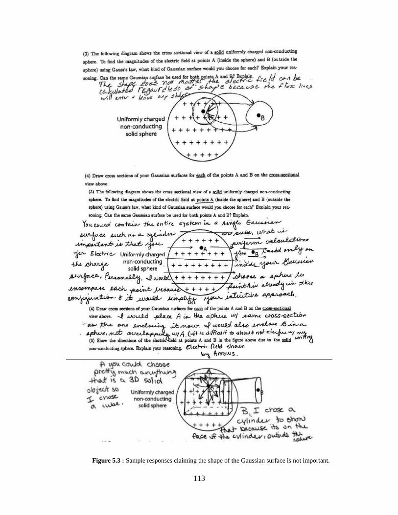
113

Figure 5.3 : Sample responses claiming the shape of the Gaussian surface is not important.

114

Many students did not even realize that the Gaussian surfaces should be through the point

where they were supposed to find the magnitude of the electric field. Some students incorrectly

situated the points where the electric field was to be determined at the center of a Gaussian

sphere or on the axis of a Gaussian cylinder they drew. For example, on the pre-test question (3)

for tutorial IV, some students claimed that points A and B should be at the center of a Gaussian

sphere, circle (which is not even a Gaussian surface), or on the axis of a Gaussian cylinder (see

Figure 5.4 as a sample response to the pre-test question (3) on tutorial IV).

Figure 5.4: A sample response claiming point A and B should be on the axis of Gaussian cylinder

Another common misconception that students had is that if they have to find the electric

field at two points A and B, e.g., inside and outside the sphere due to a uniform sphere of charge,

then there should be one hypothetical Gaussian surface drawn through both points A and B. For

example, the Gaussian surface that some students drew in pre-test question (3) for tutorial IV to

find the electric field at points A and B due to a solid uniformly charged non-conducting sphere

was a finite cylinder with both points A and B at the caps of the same cylinder (see Figure 5.5 as

a sample response to the pre-test question (3) for tutorial IV).Other students used Gaussian

115

surfaces with incorrect symmetry to find the magnitude of the electric field at points A and B in

the pre-test question (3) for tutorial IV as shown in sample Figure 5.6.

Figure 5.5 : A sample response claiming both points A and B should be on the same Gaussian surface.

116

Figure 5.6 : Sample responses with Gaussian surfaces involving incorrect symmetry to find the magnitude

of the electric field at points A and B

117

Similarly, in the post-test question (3), some students did not know that the hypothetical

Gaussian surface to find the magnitude of the electric field due to a symmetric charge

distribution should be such that the Gaussian surface passes through the point where they had to

find the magnitude of the electric field. In the tutorial group, the number of students who had

such difficulty was significantly less than in the pre-test.

5.4.10 Confusing electric flux for a vector

A common difficulty was mistakenly thinking that the electric flux is a vector. In interviews,

students justified their response about why the electric flux is a vector by using the following

facts: The expression for flux involves a scalar product of two vectors. Instead of identifying

cos with the angle between the electric field and the area vector, many students concluded that

the flux is a vector because it involves a cos . Students pointed to the fact that the electric flux

can have both positive and negative signs so it must be a vector. When asked if it would make

sense to say that the electric flux points at 030 south of west, students often avoided a direct

response. Their response implied that for a physical quantity to be a vector, it was not necessary

to be able to specify the exact direction. Rather, because the electric field lines “going out” of a

closed surface contribute positively and those “going in” contribute negatively to the total

electric flux through a closed surface, electric flux must be a vector.

5.4.11 Confusion between electric flux and electric field

Students often have difficulty distinguishing between electric field and electric flux. While the

electric field is a vector which is defined at each point, electric flux is a scalar quantity which is

118

defined through a surface. Of course, electric field and electric flux are related and students often

have difficulty understanding this relation properly. It is difficult for students to understand that

no net electric flux through a closed surface does not imply there cannot be a non-zero electric

field at each point on the surface. For example, in response to the post-test question (3) on

tutorial III, one student incorrectly noted: “Agree. No electricity with no net flux”

Tutorial III helps students learn to distinguish between electric field and electric flux.

Some students were quite assertive during interviews and incorrectly claimed that if the

magnitude of the electric flux through a closed surface is smaller than it is for another surface,

then the magnitude of the electric field at points on the surface through which the electric flux is

smaller must be smaller too. Interviews suggest that if two concentric Gaussian spheres were

drawn with a single point charge at the center, some students claimed that the electric flux

through the smaller sphere must be larger because it is closer to the positive charge at the center

although the net charge enclosed is the same for both surfaces. These students were often

confused about the distinction between electric flux and electric field. Interviews also show that

some students incorrectly claimed that the electric flux through the larger sphere must be larger

because it has a larger area although again the net charge enclosed is the same for both spheres.

A common difficulty with a question which was part of tutorial III, for which Figure 5.7

shows the setup, was assuming that the electric field is zero at point B on the side surface of the

cube, although the question explicitly mentions that the cube is in a uniform electric field of

20N/C. During the development of the tutorial, in interviews and free-response questions, some

students explicitly claimed that the area vector of the side surface is perpendicular to the

direction of the electric field lines. Therefore, the electric field must be zero at point B. This kind

of confusion between the electric field at a point and the contribution to the electric flux from a

119

certain area was quite common.

Figure 5.7 : Question on which students display confusion between electric field and electric flux.

Similar difficulty in differentiating and relating the electric field and electric flux was

manifested in response to, e.g., questions (1) and (2) on the pre-test for tutorial IV. Responses to

these questions suggest that many students are not comfortable with the statement of Gauss’s law

that relates the net flux through a closed surface to the net charge enclosed. They have difficulty

differentiating between the electric flux through a closed surface and the electric field at a point

on the surface. For example, in question (1) many students chose (I) (or (I) and (III)) and claimed

incorrectly that only those surfaces can be used to determine the net electric flux through them

because the other surfaces did not have the correct symmetry. A possible reason for this mistake

is the confusion between electric flux and electric field.

A common incorrect response for question (2) on the post-test of tutorial III was that the

net charge enclosed in a region is largest if the number of field lines penetrating the region is

greatest. Students who made this mistake did not pay attention to the direction of the electric

field lines which is crucial for determining the net flux through a closed surface and is related to

the net charge enclosed via Gauss’s law.

120

Question (5) on the post-test of tutorial III was extremely difficult and many students

incorrectly agreed with the statement. The confusion was often between the electric field and

flux and these students claimed that if there is no charge inside the Gaussian surface, the electric

field must be zero everywhere inside the hollow region. Some students incorrectly argued that

the effect of the positive charges on the surface of the sphere and the negative point charge

outside will somehow mutually cancel each other’s effect so that the net electric field inside the

non-conducting sphere is zero everywhere.

5.4.12 Confusion between open and closed surfaces and Gauss’s law

Students were sometimes unsure about the distinction between open and closed surfaces and that

Gauss’s law is only applicable to closed surfaces. For example, pre-test questions (1) and (2) in

tutorial IV at least partly assess whether students understand this distinction. Some students

incorrectly believed that Gauss’s law applies to any symmetrical surface even if it is not closed.

For example, in response to question (1), these students claimed that the electric flux due to an

infinitely long line of charge (with uniform linear charge density ) is 0/ L even for the

two-dimensional square sheet.

5.4.13 There must be a charge present at the point where the electric field is desired

Similar to the difficulty found when students worked on tutorials I and II, some students claimed

that if they are asked to find the electric field at a point A, there must be a charge present at that

point even when working on symmetry and Gauss’s law tutorials. For example, in the pre-test

question (5) for tutorial IV in which students were asked to find the electric field due to a solid

121

non-conducting sphere with uniform surface charge at a point A, some students drew electric

field lines coming out of point A as though there was a point charge located at point A and that

was the only charge that was contributing to the electric field at point A. A sample response from

a student who made such a claim is shown in Figure 5.8. Some students believed that there were

two charges with equal magnitude but opposite signs present at points A and B and they drew the

electric field lines from A to B as one would draw for a dipole because they were asked for the

electric field at two points A (inside the uniform sphere of charge) and B (outside). On the other

hand, some students claimed that the electric field at point B is zero because there is no charge at

point B since it is outside the sphere of charge.

Figure 5.8 : A sample response for the pre-test question (5) on tutorial III

5.4.14 Assuming a point charge is present if the charge distribution in a region is not given

explicitly

When students are asked questions without a concrete case (with a given charge distribution),

they sometimes assume that the charge distribution must be the simplest possible, namely, a

122

point charge. Incidentally, students who made such an assumption never said that they were

considering a very special case and in general the charge distribution could be more complex.

For example, a common problem with post-test question (1b) in tutorial III was assuming that

there was a point charge at the center of the sphere and using the given radius of the sphere to

find the electric field using Coulomb’s law.

In response to the post-test question (2d) for tutorial III, one common incorrect response

was A and C because all lines are going in or out from the center and students assumed that there

must be a point charge at the center of each of the regions A and C. For example, one student

noted: “A and C because all the flux lines seem to be directed in and out of the center of the

sphere.” One interviewed student claimed that it is easy to tell from the figure that A and C have

point charges at the center. However, there is no way to tell from the information given because

even if the electric field lines are perpendicular to a spherical surface everywhere, the hidden

charges inside could be uniformly distributed about the center of the sphere and not necessarily

be localized as point charges at the center of the sphere.

5.4.15 Difficulty visualizing in three dimensions

Some students had great difficulty visualizing in three dimensions. Some students did not distinguish

between two and three dimensional surfaces, e.g., some of them used the words sphere and circle

interchangeably or used the words cube and square interchangeably. Some students incorrectly

claimed that the Gaussian surface for a spherical charge distribution is a circle although a circle

is not a closed surface and hence cannot be a Gaussian surface. In response to question (2) on the

pre-test of tutorial IV, one interviewed student argued for a long time that the distances of all

points on the surface of the Gaussian sphere must be the same from the axis of the infinitely long

123

line (with uniform charge) similar to the distance of all points on a coaxial Gaussian cylinder. It

was clear from the discussion that the student had difficulty in visualizing how different points of

the surface of the Gaussian sphere with its diameter coinciding with the infinite line of charge

can have different distances from the axis of the cylinder. Visualizing this situation became more

difficult because the student kept confusing what was relevant for the problem with the fact that

all points on the sphere are at the same distance from the center of the sphere.

In some questions, we provided students with two views, e.g., cross-sectional view and

side view for an infinite non-conducting hollow cylinder with uniform surface charge and

infinite line with uniform charge in the pre-test question (1) of Tutorial V. Some students who

used the cross-sectional view, referred to the cross-sectional view of the cylinder as a sphere or

circle in their written explanations. There were also students who used either the cross-sectional

view to find the electric field at a point A inside the cylinder and used the side view for the

electric field at a point B outside or vice versa. Sometimes, these students incorrectly claimed

that the appropriate Gaussian surface for point A inside the cylinder is a sphere and for the point

B outside the cylinder is a cylinder (or vice versa).

5.4.16 Student difficulty with basic mathematical tools

Although the level of mathematics required to carry out Gauss’s law is not very difficult, some

students struggle with simple mathematical concepts such as the dot product of two vectors or the

conceptual understanding of a surface integral. For example, in response to question (3) on the post-

test of Tutorial III, one student wrote, “disagree, AAdEAdE 0

.” This addition,

at least in this context, is surprising since the two terms that he is adding do not even have the same

dimensions!

124

5.4.17 Student difficulty with scientific language

Physics is a discipline with precise meanings for various concepts. One common difficulty is the

imprecise language students use to express physics concepts. Part of the reason Newton’s third

law is so difficult because students have not learned to differentiate between the concepts of

“acceleration” and “force” (Halloun & Hestenes 1985, Hestenes et al 1992, Thornton & Sokoloff

1998, Hake 1998). For instance, students often believe that a large trailer truck will exert a larger

magnitude force on a small car than the car will exert on the truck. While the forces on both

objects will be equal in magnitude and opposite in direction, the acceleration is larger for the

smaller object and hence the damage to the small car may in general be larger.

We find that students sometimes have difficulty in constructing sentences that are

scientifically correct. In some cases, we could infer what students meant despite their imprecise

language. But in other cases, it was difficult to make sense of their sentence structures. For

example, in response to the post-test question (1) on tutorial III, one student incorrectly claimed:

“ cosEA . All charges are pointing perpendicular to the surface so = 0.” Prodding the

student further suggests that the student believed that the electric field at each infinitesimal area

of the surface will be parallel to the area vector which need not be true for the situation given.

Similarly, in response to question 2 on the post-test of tutorial III, a student who provided the

correct responses to parts (a) and (b), respectively, noted “[Figure] A because charge is leaving.”

and “[Figure] C because charge is coming towards the sphere”. It is clear from the student’s

response that the student is referring to the electric field lines and calling them charges. In

response to the post-test question 2(d) for tutorial III, the following examples also show similar

difficulty with the language of physics.

There could be multiple charges but the net charge is pointing in the direction indicated.

125

Yes, A and C because they have a positive or negative electric field.

In the first statement, the student is correct that there could be multiple charges but the

student talks about the net charge pointing in a certain direction which is semantically incorrect. The

second student’s response is incorrect but, additionally, the student is using scientifically

inappropriate language while talking about the electric field being positive or negative without any

coordinate axes and probably referring to electric field lines pointing outward or inward from the

closed surface.

One student who correctly disagreed with the statement in the post-test question (3) of

Tutorial III, drew a charge outside the cube as a counterexample and said, “electric field through

the cube is zero because the charge passes through the cube”. The idea the student was trying to

convey was that, since the point charge is outside the cube, all of the electric field lines entering

the cube also leave the cube so that there is no net flux through the cube. Such incorrect use of

language can significantly impede student’s ability to organize their knowledge hierarchically. In

response to the same question (3) on the post-test of tutorial III, the following sample responses

from the students also show difficulty with the language of physics:

disagree. flux could be travelling opposite of field

disagree because there must be some point on the surface of the cube that is not balanced.

I disagree. The only flux that has any effect on the object is the enclosed flux or charge.

Agree because the electric field should have the same charge as the flux running through it

Agree. The only electric flux that has any effect on the object is the charge/flux enclosed.

126

None of these sentence structures are consistent with the expert view of relevant physics

concepts.

In response to post-test question (4) for tutorial III, the following sample incorrect

responses illustrate student difficulties with language.

disagree. Flux could be negative thus exerting an inward force.

disagree because there is a uniform electric field on the surface does not always mean

there is zero flux. The sphere may contain charge and there would be flux even if field

cancels out. (Note that in this example, the student initially refers to “zero” electric field

as “uniform” electric field, which may technically be correct, but later makes an

argument that the electric flux through a sphere can be non-zero even if the electric field

everywhere on the surface is zero.)

agree because flux would be distributed evenly throughout the sphere along with the electric

field

agree because points on the sphere are not tilted in some direction.

We found it difficult to change students’ language significantly in a short period of time and

students did not easily give up using related words, e.g., “electric field lines” and ”electric charge”

interchangeably as in some of the examples above. Similarly, words such as electric force, electric

field, electric flux, and electric charge were often used interchangeably by some students. Our

preliminary analysis shows that students who do not speak the scientific language precisely and use

related terms indiscriminately usually have a much more difficult time learning relevant concepts

than others. However, further study is required to understand students’ facility with scientific

language and their ability to learn concepts well within a fixed period.

127

5.4.18 If A implies B then B must imply A or other convoluted reasoning

Students sometimes use incorrect circular reasoning, e.g., if zero electric field at each point on the

surface implies that the electric flux through the surface must be zero then zero electric flux through a

closed surface implies that the electric field must be zero at each point. In response to post-test

question (3) for tutorial III, one interviewed student incorrectly claimed: “flux is equal to the total

charge divided by 0 . If the flux is zero, then charge is zero, and so the field is zero.” While his first

statement is correct if the student is referring to the charge enclosed by the closed surface, the second

statement is incorrect because the relationship between the electric flux through a closed surface and

the electric field at various points on the surface is complicated. The following sample responses for

the same question also illustrate the tendency to over generalize:

Agree. Flux is what creates the field so if there is no flux there is no electric field.

Agree. Electric flux and field are determined only by q enclosed. Flux outside does not matter.

In response to the post-test question (4) on tutorial III, while students correctly agreed with the

statement, their reasoning is incorrect. If all the excess charge is outside the closed surface, it only

implies that the electric flux through a closed surface will be zero according to Gauss’s law and not

the electric field at various points on the surface. The following sample responses illustrate such

responses:

agree. The excess charge must be in the exterior.

agree because if the net charge inside is zero then both the flux and field at the surface will be

zero.

128

In response to the post-test Question (5) for tutorial III, here is an example of a circular

reasoning: “agree. The ball must have a net charge inside of it for there to be a net flux which means

there can’t be a net electric field if no charge inside.”

Such convoluted reasoning is common in physics especially amongst introductory physics

students because physics is abstract and proper reasoning about abstract concepts is difficult.

Students need guidance and support with concrete examples in different contexts to internalize

various abstract physics concepts. The following Wason tasks (Wason 1968) are examples from

cognitive psychology of abstract and concrete problems which are conceptually similar, but the

abstract problem is cognitively more demanding.

Abstract Task: You will lose your job unless you enforce the following rule: “If a person

is rated K, then his/her document must be marked with a 3”.

Each card on the table for a person has a letter on one side and a number on the

other side.

Indicate only the card(s) shown in Figure 5.9 that you definitely need to turn over

to see if the document of any of these people violates this rule.

Concrete Task: You are serving behind the bar of a city center pub and will lose your job

unless you enforce the following rule: “If a person is drinking beer, then he/she must be

over 18 years old”.

Each person has a card on the table which has his/her age on one side and the name of

his/her drink on the other side. Indicate only the card(s) shown in Figure 5.10 that you definitely

need to turn over to see if any of these people are breaking this rule.

129

Figure 5.9 : Figure for Wason Task in abstract context (Wason 1968).

Figure 5.10 : Figure for Wason Task in concrete context (Wason 1968).

The correct answer for the abstract case is that you must turn the cards with K and 7 (to make

sure that there is no K on the other side). Note that the logic presented in the task is one sided in that

it is okay for a document with a 3 to have anything on the other side. The correct answer for the

concrete case is “beer” and “16 years old”, and it is much easier to identify these correct answers

than the correct answers for the abstract case. Typically, people find the abstract Wason task difficult

the first time they encounter it but not as difficult in subsequent encounters. One implication for

teaching abstract concepts of physics is that once the instructor has built an intuition about a set of

related concepts, the concepts may not appear difficult to him/her even if they are abstract. In such

situations, the instructor may overlook the cognitive complexity of the problem for a beginning

student unless the instructor puts himself/herself in the students’ shoes. Tutorials provide scaffolding

to help students develop a robust knowledge structure so that there is less possibility for students

reasoning in a convoluted manner.

130

5.5 PERFORMANCE OF TUTORIAL AND CONTROL GROUPS

Table 5.1 shows the student performance (on each question and also overall) on the pre-test and

post-test in each of the three tutorials (III-V) in percentage for each class. The classes utilizing

each tutorial may differ either because additional pre-/post-test questions were added or the pre-

test for tutorial V was not administered to some of the classes. The differences in the

performance of different classes may also be due to the differences in student samples,

instructor/TA differences or the manner in which the tutorials were administered.

Table 5.1 : Average percentage scores obtained on individual questions on the pre-/post-tests for tutorial classes

Tutorial Class n

Pre-test Post-test

1 2 3 4 5 6 Pre-

total 1 2 3 4 5 6

Post-

total

III

1 86 48 - - - - - 48 79 86 73 93 83 - 83

2 62 49 - - - - - 49 78 90 83 98 - - 86

3 63 55 - - - - - 55 83 80 85 96 88 - 86

IV

1 64 41 19 53 54 43 3 37 86 84 92 95 96 86 90

2 51 30 8 57 29 - - 31 88 91 88 54 - - 87

3 65 29 22 58 58 41 18 40 83 91 96 92 91 92 91

V

1 87 - - - - - - - 69 59 68 69 96 73 70

2 57 20 26 35 - - - 27 82 76 85 - - - 81

3 65 - - - - - - - 93 81 90 91 98 92 90

Table 5.2 shows the pre-/post-test data from a comparison group which consists of a class

in which tutorials III-V were not used. The total class time devoted to these topics was

equivalent to the classes in which the tutorials were administered. In the tutorial classes,

instructors did not do some of the examples but let the students do them as part of the tutorials to

save time. The pre-tests were given to the students in the comparison group immediately after

relevant instruction but post-tests were given in the following week as part of the weekly

131

recitation quizzes after the students had the opportunity to complete all the homework problems

from those topics.

Table 5.2 : Average percentage scores obtained on individual questions on the pre-/post-tests for the non-tutorial

class.

Tutorial n Pre-test Post-test

1 2 3 4 5 6 Pre-total 1 2 3 4 5 6 Post-total

III 59 43 - - - - - 43 36 70 72 72 28 - 56

IV 69 33 13 52 36 46 12 34 45 59 51 51 45 26 43

V 57 18 11 49 - - - 24 18 19 44 27 69 34 35

Table 5.3 shows the p values obtained by comparing the performance of tutorial classes

and non-tutorial class on the pre-/post-tests. The results of Table 5.1-5.3 indicate that regardless

of whether the students belonged to the tutorial or comparison groups, their performance on the

pretest was poor after traditional instruction. However, students in the comparison group did

significantly worse on the post-test than the classes in which students worked on the tutorials.

Table 5.3 : P value for t-tests comparing performance of tutorial classes and non-tutorial classes on the pre-/post-

tests.

P value Tutorial III Tutorial IV Tutorial V

pre-test 0.32 0.52 0.60

post-test 0.00 0.00 0.00

Table 5.4 shows the performance of students on the pre-/post-tests for each tutorial

partitioned into three separate groups based upon the pre-test performance (see the Range

column). As can be seen from Table 5.4, tutorials generally helped all students including those

who performed poorly on the pre-test.

132

Table 5.4 : Percentage average pre-/post-test scores (matched pairs) in tutorial classes for each of the three tutorials

(III-V), divided into three groups according to the pre-test performance.

N Tutorial Range (%) n1 (class 1) pre post n2 (class 2) pre post n3 (class 3) pre post

211 III

All 86 48 83 62 49 86 63 55 86

0-34 30 18 80 23 21 84 21 16 85

34-67 39 52 83 26 55 87 19 53 85

67-100 17 92 86 13 86 89 23 92 89

180 IV

All 64 37 90 51 31 87 65 40 91

0-34 31 17 86 30 16 83 26 15 88

34-67 29 51 94 14 44 92 31 49 91

67-100 4 78 94 7 64 93 8 85 97

57 V

All

57 27 81

0-34

43 14 78

34-67

9 48 90

67-100

5 96 92

Table 5.5 shows the performance of students in the comparison group on the pre-/post-

tests for each tutorial partitioned into three separate groups based upon the pre-test performance.

As can be seen from comparing Tables 5.4 and 5.5, students in the comparison group for none of

the pre-test range performed on par with the tutorial groups on the post-tests.

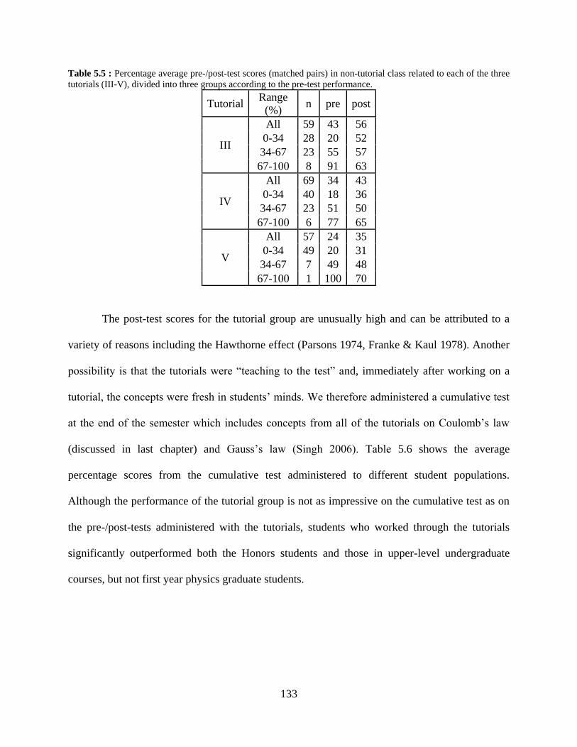
133

Table 5.5 : Percentage average pre-/post-test scores (matched pairs) in non-tutorial class related to each of the three

tutorials (III-V), divided into three groups according to the pre-test performance.

Tutorial Range

(%) n pre post

III

All 59 43 56

0-34 28 20 52

34-67 23 55 57

67-100 8 91 63

IV

All 69 34 43

0-34 40 18 36

34-67 23 51 50

67-100 6 77 65

V

All 57 24 35

0-34 49 20 31

34-67 7 49 48

67-100 1 100 70

The post-test scores for the tutorial group are unusually high and can be attributed to a

variety of reasons including the Hawthorne effect (Parsons 1974, Franke & Kaul 1978). Another

possibility is that the tutorials were “teaching to the test” and, immediately after working on a

tutorial, the concepts were fresh in students’ minds. We therefore administered a cumulative test

at the end of the semester which includes concepts from all of the tutorials on Coulomb’s law

(discussed in last chapter) and Gauss’s law (Singh 2006). Table 5.6 shows the average

percentage scores from the cumulative test administered to different student populations.

Although the performance of the tutorial group is not as impressive on the cumulative test as on

the pre-/post-tests administered with the tutorials, students who worked through the tutorials

significantly outperformed both the Honors students and those in upper-level undergraduate

courses, but not first year physics graduate students.

134

Table 5.6 : The average percentage of correct responses to each of the 25 questions on the cumulative test (Singh

2006) for different student population.

Without

Tutorial

Honors

Students

Upper-level

Undergrad With

Tutorial

Graduate

Students Pre Post

Q N=135 N=182 N=33 N=28 N=278 N=33

1 56 44 42 53 60 73

2 45 64 52 57 84 64

3 23 57 61 61 70 79

4 22 31 33 39 67 73

5 82 77 70 68 84 88

6 60 55 82 82 69 76

7 69 73 64 68 79 91

8 37 38 52 32 68 88

9 61 53 67 68 66 91

10 41 46 45 50 56 70

11 46 25 24 68 72 94

12 45 35 43 53 69 79

13 3 19 18 14 26 36

14 54 49 55 64 72 85

15 23 26 36 25 52 61

16 13 14 9 36 45 52

17 15 25 27 7 45 45

18 40 28 58 39 63 73

19 42 66 64 53 58 94

20 52 45 55 53 47 94

21 20 43 36 53 34 88

22 21 30 27 50 46 73

23 34 55 42 53 62 82

24 22 32 18 61 38 55

25 22 31 27 28 40 55

Avg 38 42 44 49 59 75

p 0.00 0.00 0.00 0.053 0.00

135

5.6 CONCLUSION

We have developed and evaluated tutorials to help calculus-based introductory students learn about

symmetry and Gauss’s law. Pre-/post-tests for each tutorial suggest that the tutorials can be effective

in improving student understanding of these concepts. Students in four different classes who used the

tutorials performed significantly better on a cumulative test related to these topics than even the

students in the upper-level electricity and magnetism undergraduate course.

5.7 ACKNOWLEDGEMENTS

We are very grateful to Z. Isvan for help in grading and analyzing the pre-/post-test data. We thank F.

Reif, R. P. Devaty and J. Levy for helpful discussions. We thank all the faculty who helped in this

study by administering the tutorials and/or pre-/post-tests to their classes.

5.8 REFERENCES

Bilak, J. & Singh, C. (2007). “Improving Students’ Conceptual Understanding of Conductors

and Insulators”, Proceedings of the Phys. Ed. Res. Conference, Greensboro, NC, (L. Hsu,

L. Mc-Cullough, C. Henderson Eds.), AIP Conf. Proc. 951, 49-52.

Brown, A.(1978). “Knowing when, where and how to remember: A problem of metacognition”.

In Ed. R. Glaser, Advances in instructional psychology, Hillsdale, NJ: Lawrence

Erlbaum.

Chi, M. T. H. (1994) “Thinking aloud”. In M. W. van Someren, Y. F. Barnard, &J. A. C.

Sandberg, The Think Aloud Method, Chap. 1. London: Academic Press.

Hake, R. R. (1998). “Interactive-engagementversus traditional methods: A six-thousand-student

survey of mechanics test data for introductory physics courses”, Am. J. Phys. 66, 64.

136

Halloun, I. & Hestenes, D.(1985). “The initial knowledge state of college physics students”, Am.

J. Phys. 53, 1043.

Hestenes, D., Wells, M. & Swackhamer, G. (1992). “Force Concept Inventory,” Phys. Teach. 30,

141.

Franke, R. H. & Kaul, J. D. (1978). “The Hawthorne experiments: First statistical interpretation”,

American Sociological Review, 43, 623-643.

National Research Council (1999a), How people learn: Brain, mind, experience and school.

Committee on developments in science on learning. Edited by J. Bransford, A. Brown

and R. Cocking. Washington, DC: National Academy Press.

National Research Council (1999b). How people learn: Bridging research and practice.

Committee on learning research and educational practices. Edited by M. Donovan, J.

Bransford, and J. Pellegrino. Washington, DC: National Academy Press.

Newell, A. (1990) Unified theories of cognition, Cambridge, MA: Harvard University Press.

Parsons, H. M. (1974). “What happened at Hawthorne?”, Science, 183(4128), 922-932.

Posner, G., Strike, K., Hewson, P. & Gertzog, W. (1982). “Accommodation of a scientific

conception: Toward a theory of conceptual change”, Science Education, 66, 211-227.

Schoenfeld, A. (1987). “What’s all the fuss about metacognition?”. In A. Schoenfeld (Ed),

Cognitive science and mathematics education. Hillsdale NJ: Lawrence Erlbaum; Davis,

E. (1997). “Metacognitive scaff olding to foster scientific explanations”, paper at the

annual meeting of American Educational Research Association, New York: NY.

Simon, H. and Kaplan, C. (1989). Foundations of cognitive science. Edited by M. I. Posner. MIT

press.

Singh, C. (2006). “Student understanding of Symmetry and Gauss’s law of electricity”, Am. J.

Phys., 74(10), 923-236.

Thornton, R. & Sokoloff, D. (1998). “Assessing student learning of Newton’s laws: The force

and motion conceptual evaluation and the evaluation of active learning laboratory and

lecture curricula,” Am. J. Phys. 66, 338.

Wason, P. (1968). “Reasoning about a rule”, Quarterly Journal of experimental psychology, 20,

273281; Wason, P. & Johnson-Laird, P. (1972). Psychology of reasoning: Structure and

content, Cambridge, MA: Harvard University Press.

137

6.0 DEVELOPING A MAGNETISM CONCEPTUAL SURVEY

6.1 ABSTRACT

We discuss the development and evaluation of a research-based conceptual multiple-choice

survey related to magnetism, students’ difficulties related to magnetism concepts and the

performance of introductory students on the test before and after traditional instructions. We also

discuss the performance of the upper level undergraduates and graduate students. We compare

the performance of students from algebra-based classes and calculus-based classes and find that

calculus-based students outperformed algebra-based students on the conceptual test both before

and after traditional instruction. We also discuss the use of the survey to investigate gender

differences in students' difficulties with concepts related to magnetism. We find that while there

was no gender difference on the pre-test, female students performed significantly worse than

male students when the survey was given as a post-test in traditionally taught calculus-based

introductory physics courses (similar results in both the regular and honors versions of the

course). In the algebra-based courses, the performance of the female students and the male

students has no statistical difference on the pre-test or the post-test. We compare algebra-based

and calculus-based students’ performance on MCS both as a pre-test and a post-test. Significant

difference appeared on the pre-test and persisted on the post-test. We also compare students’

performance on MCS with their performance on CSEM. We find that students performed slightly

better on CSEM.

138

6.2 INTRODUCTION

Research-based multiple-choice tests can be useful tools for surveying student learning in

physics courses. They are easy and economical to administer and to grade, have objective

scoring, and are amenable to statistical analysis that can be used to compare student populations

or instructional methods. A major drawback is that the thought processes are not revealed by the

answers alone. However, when combined with student interviews, well-designed tests are

powerful tools for educational assessment. A number of multiple-choice tests have been

developed and widely used by physics instructors to measure students’ conceptual learning in

physics courses. A commonly used research-based multiple-choice test for mechanics is the

Force Concept Inventory (FCI) (Hestenes, et al. 1992). In Electricity and Magnetism (E&M), the

CSEM and BEMA surveys have been developed which cover E&M concepts discussed in

introductory courses (Maloney et al. 2001, Ding et al. 2006).

Magnetism is an important topic in introductory physics. We developed a research-based

30 item multiple-choice test on magnetism (called the Magnetism Conceptual Survey or MCS) to

explore the difficulties students have in interpreting magnetism concepts and in correctly

identifying and applying them in different situations. The identification of student difficulties

with magnetism for these various groups can help in designing instructional tools to address the

difficulties. We also wish to know the extent to which the difficulties are universal, and if there

is a correlation with instructor or student preparation and background, e.g., whether they are in

the calculus-based or algebra-based courses or whether they are females or males.

Previous research shows that there is often a gender difference in student performance in

mathematics and other disciplines (Hyde et al. 1990, Kahle & Meece 1994) as well as in physics

(Lorenzo et al. 2006, Pollock et al. 2007, Kost et al. 2009, Kohl & Kuo 2009, Kost et al. 2009)

139

which can sometimes be reduced by carefully designed curricula. Here, we explore gender

difference in student understanding of magnetism concepts covered in introductory physics

courses by surveying students in the calculus- and algebra-based courses using the MCS as a pre-

test and a post-test (before and after instruction in relevant concepts).

6.3 MAGNETISM CONCEPTUAL SURVEY DESIGN

The Magnetism Conceptual Survey (MCS) covers topics in magnetism discussed in a traditional

calculus- or algebra-based introductory physics curriculum up to Faraday’s law. During the test

design, we paid particular attention to the important issues of reliability and validity (Ding et al.

2006). Reliability refers to the relative degree of consistency in scores between testing if the test

procedures are repeated in immediate succession for an individual or group. On a reliable survey,

students with different levels of knowledge of the topic covered should perform according to

their mastery. In our research, we use the data collected to perform statistical tests to ensure that

the survey is reliable within the classical test theory. For example, the reliability index measures

the internal consistency of the whole test (Ding et al. 2006). One commonly used index of

reliability is KR-20 which is calculated for the survey as a whole (Ding et al. 2006).

Validity refers to the appropriateness of the test score interpretation (Ding et al. 2006). A

test must be reliable for it to be valid for particular use. The design of the MCS test began with

the development of a test blueprint that provided a framework for planning decisions about the

desired survey attributes. We tabulated the scope and extent of the content covered and the level

of cognitive complexity desired. During this process, we consulted with several faculty members

140

who teach introductory E&M courses routinely about concepts they believed their students

should know about magnetism.

We classified the cognitive complexity using a simplified version of Bloom’s taxonomy:

specification of knowledge, interpretation of knowledge and drawing inferences, and applying

knowledge to different situations. Then, we outlined a description of conditions/contexts within

which the various concepts would be tested and a criterion for good performance in each case.

The tables of content and cognitive complexity along with the criteria for good performance

were shown to three physics faculty members at the University of Pittsburgh (Pitt) for review.

Modifications were made to the weights assigned to various concepts and to the performance

criteria based upon the feedback from the faculty about their appropriateness. The performance

criteria were used to convert the description of conditions/contexts within which the concepts

would be tested to make free-response questions. These questions required students to provide

their reasoning with the responses.

The multiple-choice questions were then designed. The responses to the free-response

questions and accompanying student reasoning along with individual interviews with a subset of

students guided us in the design of good distracter choices for the multiple-choice questions. In

particular, we used the most frequent incorrect responses in the free-response questions and

interviews as a guide for making the alternative distracter choices. Four alternative choices have

typically been found to be optimal, and we chose the four distracters to conform to the common

difficulties to increase the discriminating properties of the items. Three physics faculty members

were asked to review the multiple-choice questions and comment on their appropriateness and

relevance for introductory physics courses and to detect ambiguity in item wording. They went

over several versions of the survey to ensure that the wording was not ambiguous. Moreover,

141

several introductory students were asked to answer the survey questions individually in

interviews to ensure that the questions were not misinterpreted.

6.4 MCS ADMINISTRATION

The final version of the MCS was administered both as a pre-test and a post-test to a large

number of students at Pitt. These students were from three traditionally taught algebra-based

classes, and eight regular (in contrast to the honors) calculus-based introductory classes. In our

analysis presented here for the reliability index KR-20, the item difficulty and discrimination

indices, and point biserial coefficient of the items, we kept only those students who took the

survey both as a pre-test and a post-test except in one algebra-based class. In that class, most of

the students who worked on the survey did not provide their names and seven more students

participated in the post-test than the pre-test. Thus, in the algebra-based course, 267 students

took the pre-test, and 273 students took the post-test. In the regular calculus-based courses, 575

students took both the pre-test and the post-test.

Pre-tests were administered in the first lecture or recitation at the beginning of the

semester in which students took introductory second semester physics with E&M as a major

component. The students were not allowed to keep the survey. Post-tests were administered in

the recitations after instruction in all relevant concepts on magnetism covered in the MCS.

Students were typically asked to work on the survey for a full class period (40-50 minutes).

The KR-20 for the combined algebra-based and calculus-based data is 0.83, which is

reasonably good by the standards of test design (Ding et al. 2006). The MCS was also

administered to 42 physics graduate students enrolled in a first year course for teaching assistants

to bench mark the performance that can be expected of the undergraduate students. The average

score for the graduate students is 83% with a KR-20 of 0.87.

142

The item difficulty is a measure of the difficulty of a single test question (Ding et al.

2006). It is calculated by taking the ratio of the number of correct responses on the question to

the total number of students who attempted to answer the question. Figure 6.1 shows the

difficulty index for each item in the survey for the sample of 848 students obtained by combining

the algebra-based and calculus-based classes. The average difficulty index is 0.46 which falls

within the desired criterion range (Ding et al. 2006). The average difficulty index for the algebra-

based class is 0.45 which is lower than 0.53 for the calculus-based class.

Figure 6.1 : Difficulty index for various items in the MCS

The item discrimination index measures the discriminatory power of each item in a test

(Ding et al. 2006). A majority of the items in a test should have relatively high discrimination

indices to ensure that the test is capable of distinguishing between strong and weak mastery of

the material. A large discrimination index for an item indicates that students who performed well

on the test overall performed well on that item. The average item discrimination index for the

combined 848 students sample including all items on the MCS is 0.33 which is reasonable from

the standards of test design (Ding et al. 2006). Figure 6.2 shows that for this sample the item

discrimination indices for 22 items are above 0.3. The average discrimination index for the

algebra-based class is 0.29 and for the calculus-based class it is 0.33.

143

Figure 6.2 : Discrimination index for the MCS items

The point biserial coefficient is a measure of consistency of a single test item with the

whole test (Ding et al. 2006). It is a form of a correlation coefficient which reflects the

correlation between students’ scores on an individual item and their scores on the entire test. The

widely adopted criterion for a reasonable point biserial index is 0.2 or above (Ding et al. 2006).

The average point biserial index for the MCS is 0.42. Figure 6.3 shows that all items have a point

biserial index equal to or above 0.2.

Figure 6.3 : Point biserial coefficient for the MCS items

6.5 DISCUSSION OF STUDENT DIFFICULTIES

The magnetism topics covered in the test include magnitude and direction of the magnetic field

produced by current carrying wires, forces on current carrying wires in an external magnetic

field, force and trajectory of a charged particle in an external magnetic field, work done by the

144

external magnetic field on a charged particle, magnetic field produced by bar magnets, force

between bar magnets and static charges. Table 6.1 shows the concepts that were addressed by the

various questions in the test. This is one of the several ways of classifying questions. This

classification does not necessarily reflect the way physics experts would classify the questions.

For example, one of the concept categories in which we placed Problem 9, 13, and 17 is “motion

doesn’t necessarily cause force.” As shown in Table 6.2 and 6.3, one of the common

misconceptions in Problem 9 was due to the assumption that there was force due to the particle’s

initial velocity. In Problem 13, the most common incorrect response was choice (c) because

students believed that since the magnetic field points opposite to the particle’s direction of

motion, there must be a force due to the magnetic field to decrease the speed of particle. The

most common incorrect response for Problem 17 was choice (a), which also arose due to the

incorrect belief that there must be a force or a component of force in the direction of motion.

Similarly, we classified Problem 22, 23, and 24 in the same concept category “distinguishing

between current carrying wires pointing into/out of the page and static point charges” because

many students misinterpreted the representation of current carrying wires pointing into or out of

the page as positive or negative charges.

145

Table 6.1 : Concepts covered and the questions that addressed them in the test

Concepts Question Numbers

Magnetic force on bar magnets 1, 2, 3

Distinguishing between charges and magnetic poles 4, 5, 6

Direction of magnetic field inside/outside a bar magnet 7,8

Forces on a charged particle in a magnetic field and other fields 15, 18, 19, 26

Motion doesn’t necessarily imply force 9, 13, 17

Direction of motion or magnetic force on a moving charged particle in a magnetic field 10, 14, 16, 17

Work done by magnetic force 11, 12

Forces on current carrying wires in a magnetic field 21, 25, 27

Distinguishing between current carrying wires pointing into/out of the page and static

point charges 22, 23, 24

Magnetic field generated by current loops 28, 29, 30

The average score of the algebra-based courses was 24% as a pre-test and 41% as a post-

test. In calculus-based courses, the average pre-test score was 28% and post-test score was 49%.

Table 6.2 and 6.3 shows the percentage of students who selected the choices (a)–(e) on Problems

1–30. The correct response for each question has been underlined. Table 6.2 includes the results

from algebra-based courses on both the pre- and post-test. Table 6.3 contains the pre- and post-

test results for calculus-based courses. The correct responses are italicized and bolded. Although

some questions have a strong single distractor, others have several distractor choices that are

equally popular.

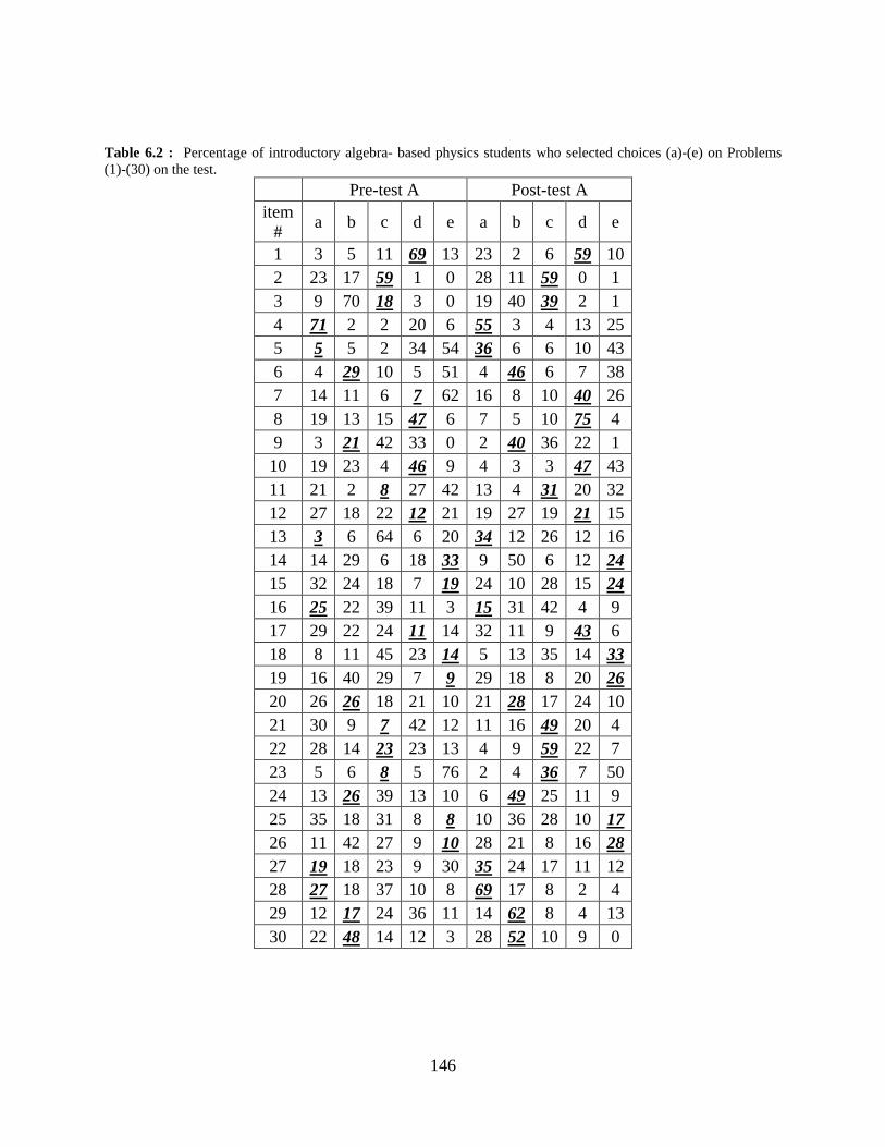
146

Table 6.2 : Percentage of introductory algebra- based physics students who selected choices (a)-(e) on Problems

(1)-(30) on the test.

Pre-test A Post-test A

item

# a b c d e a b c d e

1 3 5 11 69 13 23 2 6 59 10

2 23 17 59 1 0 28 11 59 0 1

3 9 70 18 3 0 19 40 39 2 1

4 71 2 2 20 6 55 3 4 13 25

5 5 5 2 34 54 36 6 6 10 43

6 4 29 10 5 51 4 46 6 7 38

7 14 11 6 7 62 16 8 10 40 26

8 19 13 15 47 6 7 5 10 75 4

9 3 21 42 33 0 2 40 36 22 1

10 19 23 4 46 9 4 3 3 47 43

11 21 2 8 27 42 13 4 31 20 32

12 27 18 22 12 21 19 27 19 21 15

13 3 6 64 6 20 34 12 26 12 16

14 14 29 6 18 33 9 50 6 12 24

15 32 24 18 7 19 24 10 28 15 24

16 25 22 39 11 3 15 31 42 4 9

17 29 22 24 11 14 32 11 9 43 6

18 8 11 45 23 14 5 13 35 14 33

19 16 40 29 7 9 29 18 8 20 26

20 26 26 18 21 10 21 28 17 24 10

21 30 9 7 42 12 11 16 49 20 4

22 28 14 23 23 13 4 9 59 22 7

23 5 6 8 5 76 2 4 36 7 50

24 13 26 39 13 10 6 49 25 11 9

25 35 18 31 8 8 10 36 28 10 17

26 11 42 27 9 10 28 21 8 16 28

27 19 18 23 9 30 35 24 17 11 12

28 27 18 37 10 8 69 17 8 2 4

29 12 17 24 36 11 14 62 8 4 13

30 22 48 14 12 3 28 52 10 9 0

147

Table 6.3 : Percentage of introductory calculus- based physics students who selected choices (a)-(e) on Problems

(1)-(30) on the test.

Pre-test C Post-test C

item

# a b c d e a b c d e

1 11 2 8 67 12 2 2 5 78 13

2 23 12 64 1 1 12 8 80 1 0

3 10 52 36 1 0 5 40 55 0 0

4 53 8 4 24 12 71 3 2 17 6

5 10 6 5 24 54 40 4 4 11 42

6 5 22 8 5 59 3 38 5 5 49

7 11 16 11 11 51 3 3 19 35 40

8 14 20 8 49 8 7 8 6 77 2

9 2 36 25 35 2 2 61 20 16 2

10 18 9 3 49 21 6 3 3 55 32

11 23 5 13 27 32 17 3 40 19 21

12 24 21 20 17 19 17 24 16 33 11

13 13 15 56 8 9 59 3 24 9 6

14 11 29 4 15 41 5 46 3 9 37

15 32 24 17 11 16 19 13 24 17 27

16 29 25 35 7 4 45 19 31 3 3

17 35 18 23 14 10 28 11 14 44 3

18 11 8 50 14 17 4 9 26 10 51

19 16 33 28 11 12 19 24 10 20 27

20 23 24 18 25 11 16 34 17 26 7

21 22 19 17 29 13 11 22 54 8 6

22 17 11 34 30 8 4 4 60 29 4

23 8 9 16 6 61 2 2 50 6 41

24 10 30 41 13 7 6 47 33 10 5

25 26 20 38 9 7 7 25 35 12 21

26 15 39 25 8 12 20 27 7 16 30

27 22 23 21 15 20 44 21 12 10 14

28 36 16 20 9 19 70 9 5 2 14

29 19 26 23 22 11 17 52 6 5 21

30 22 40 20 15 4 28 54 10 8 1

Below, we discuss students’ difficulties observed in understanding concepts on

magnetism. The magnetism conceptual survey (MCS) is included in the Appendix for reference.

148

6.5.1 Magnetic force between bar magnets

Problems 1-3 are related to magnetic force on bar magnets. The most common distracter in

Problem 1 was (e). Some students claimed that the net force on the middle bar magnet should be

zero because the forces due to the bar magnets on the sides should cancel out. When students

saw that there are two magnets on each side of a magnet they immediately concluded that the

forces due to the magnets are opposite to each other and therefore there is no net force on the bar

magnet. Students often did not bother to draw a free body diagram to determine the directions for

forces due to the individual bar magnets. From the students’ responses it appears that many

students did not consider Newton’s Third Law when they answered the questions. In Problem 2,

whether there is a third bar magnet or not, due to Newton’s Third Law, the force magnet 1 exerts

on magnet 2 should be equal in magnitude to the force magnet 2 exerts on magnet 1. However,

the appearance of the third bar magnet made many students think that the force with which

magnet 1 repels magnet 2 is half or twice the force with which magnet 2 repels magnet 1. In

Problem 3, the most common incorrect choice was (b). Because it is mentioned in the problem

that Magnet 1 is twice as strong as magnet 2, some students intuitively thought that the stronger

the bar magnet, the larger the force due to that bar magnet.

6.5.2 Distinguishing between magnetic poles and charges

Problems 4-6 exemplified students’ difficulties in distinguishing between the north and south

poles and localized positive and negative charges or between an electric dipole and a magnetic

dipole. When considering these types of questions, many students claimed that a bar magnet is

an electric dipole with positive and negative charges located at the north and south poles. Thus,

149

they incorrectly believed that a bar magnet can exert force on static charges or conductors. In

Problem 4, some students considered the north pole of the bar magnet as consisting of positive

charges which can induce negative charges on the conductor. Hence, they claimed that the bar

magnet exerts a force on the conductor toward the magnet. In Problem 5, students had a similar

difficulty. In the post-test, more than 40% of the students chose distracter (e), because they

considered the north pole as a positive charge which repels another positive charge. This type of

confusion was even more prevalent in Problem 6. On the post-test, 38% of the calculus-based

students answered problem 6 correctly which is not significantly different from the pre-test

performance of 22% (before instruction). The most common incorrect response was option (e),

i.e., there is no net force on charge q0. Both written explanations and interviews suggest that

students often considered a bar magnet as an electric dipole. When the interviewer asked them

whether a magnet will retain its magnetic properties when broken into two pieces by cutting it at

the center, most of them claimed that the magnetic properties will be retained, and each of the

two smaller pieces will become a magnet with opposite poles at the ends. When the interviewer

asked how that is possible if they had earlier claimed that the north and south poles are

essentially localized opposite charges, some students admitted they were unsure about how to

explain the development of opposite poles at each end of the smaller magnets but others

provided creative explanations about how charges will move around while the magnet is being

cut into two pieces to ensure that each of the cut pieces has a north and south pole. During the

interviews, we probed how students developed the misconception that a bar magnet must have

opposite charges localized at the two poles because when a child plays with a bar magnet, he/she

does not necessarily think about localized electric charges at the end. Some students claimed that

they learned it from an adult while he/she tried to explain why a bar magnet behaves the way it

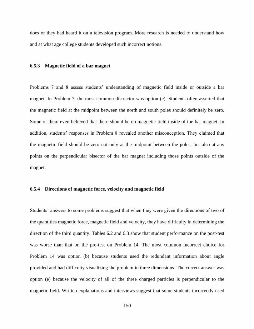
150

does or they had heard it on a television program. More research is needed to understand how

and at what age college students developed such incorrect notions.

6.5.3 Magnetic field of a bar magnet

Problems 7 and 8 assess students’ understanding of magnetic field inside or outside a bar

magnet. In Problem 7, the most common distractor was option (e). Students often asserted that

the magnetic field at the midpoint between the north and south poles should definitely be zero.

Some of them even believed that there should be no magnetic field inside of the bar magnet. In

addition, students’ responses in Problem 8 revealed another misconception. They claimed that

the magnetic field should be zero not only at the midpoint between the poles, but also at any

points on the perpendicular bisector of the bar magnet including those points outside of the

magnet.

6.5.4 Directions of magnetic force, velocity and magnetic field

Students’ answers to some problems suggest that when they were given the directions of two of

the quantities magnetic force, magnetic field and velocity, they have difficulty in determining the

direction of the third quantity. Tables 6.2 and 6.3 show that student performance on the post-test

was worse than that on the pre-test on Problem 14. The most common incorrect choice for

Problem 14 was option (b) because students used the redundant information about angle

provided and had difficulty visualizing the problem in three dimensions. The correct answer was

option (e) because the velocity of all of the three charged particles is perpendicular to the

magnetic field. Written explanations and interviews suggest that some students incorrectly used

151

the superfluous information provided about the angles that the charged particles (1) and (3) make

with the horizontal. During interviews, only when the students choosing option (b) were asked

explicit questions about the direction of the magnetic field, velocity and the angle between them

for particles (1) and (3), did they realize that the angle between them is 900 in all three cases. The

fact that these students initially claimed that the angle between the magnetic field and velocity

vector is 450 for particles (1) and (3) is similar to our finding in mechanics. In the context of

kinematics, when introductory physics students were asked a question about a rabbit's motion

whose ears were at 450

angle to the horizontal, approximately one third of the introductory

students used this redundant information about the angle of the rabbit's ears to solve the problem

incorrectly. In Problem 17, the calculus-based student performance on this question changed

from 14% on pre-test to 44% on post-test. It is similar to the performance of algebra-based

students. The most common incorrect response to this question was option (a) (but options (b)

and (c) were also chosen). In written explanations, students who chose option (a) often

incorrectly claimed that the velocity of a charged particle and the magnetic force can be at any

angle to each other, but some claimed that the magnetic field and force must be perpendicular

while others said that the field and force must be parallel. In interviews, students who provided

incorrect responses were asked to write down an expression for the magnetic force on the

charged particle in an external magnetic field. Approximately half of the students were unable to

write the correct expression. Those who wrote the correct expression were explicitly asked about

the cross product between the velocity and magnetic field and what it implies about the angle

between the magnetic force and the velocity or the magnetic field vector. Approximately half of

these students corrected their initial error and said that the cross product implies that the

magnetic force must be perpendicular to both the velocity and the magnetic field. Others did not

152

know that the cross product of two vectors must be perpendicular to each of the vectors. In

Problem 10, the most common distracter was option (e). It suggests that students have difficulty

in realizing that for electrons the direction of motion while applying the right hand rule should be

opposite to the direction for positive charges. This is also one of the difficulties students display

on Problem 20. On Problem 20, students must first use the relation between the radius of the

trajectory and the mass of a particle to determine whether this particle is an electron or proton.

Then, based on this information, they can determine the direction of motion. Students’ chose

options (a) – (d) with almost equal probability. Interview and written explanations suggest that

students have difficulty in deducing the relation between the radius of trajectory and the mass of

a particle. Some students never thought of using this relation to solve the problem. There were

also some students who correctly found that the particle is an electron. However, they incorrectly

chose option (d) because of a difficulty similar to that discussed with Problem 10.

6.5.5 Work done by magnetic force

Problem 11 and 12 are related to the work done by the magnetic field. They also probe the extent

to which students understand that magnetic force is perpendicular to velocity and only change

the direction of motion of a charge. In Problem 11 and 12, the distracters were equally popular.

Some students claimed that the work done by the magnetic force is always positive while other

students believed that it can be positive or negative depending on the charge or the orientation of

the initial velocity. Some students referred to the equation relating work to the inner product of

force and displacement to solve for work. However, they did not realize that the magnetic force

is always perpendicular to the direction of motion. As a result, they often believed that the

directions of force and velocity can form any angle and the magnetic force can do work.

153

6.5.6 Movement doesn’t necessarily imply force

Previous research in mechanics shows that students often believe that motion always implies a

force in the direction of motion. Our findings are consistent with previous research. In Problem

9, the most common incorrect option was (c), i.e., there is a force due to the electron’s initial

velocity. Another common incorrect option was (d). In response to the Problem 13, students

performed significantly better on the post-test compared to pre-test. The most common incorrect

response to Problem 13 was option (c) followed by options (d) and (e). Interviewed students

were asked such questions in the context of a lecture-demonstration related to the effect of

bringing a powerful bar magnet from different angles towards an electron beam (including the

case where the magnetic field and velocity vectors are collinear as in Problem 13). Students

were explicitly told to predict the outcome for both the electron beam and a beam of positive

charges. Students who incorrectly chose option (c) in Problem 13 explained that the particle will

slow down because the magnitude of the magnetic field is opposite to the direction of velocity

and this implies that the force on the charged particle must be opposite to the velocity. Of course,

this prediction could not be verified by performing the experiment. Students who chose options

(d) or (e) often incorrectly remembered the right hand rule about magnetic force being

perpendicular to magnetic field and provided animated explanations such as “Oh, the electron

wants to get out of the way of the magnetic field and that's why it bends”. They were surprised

to observe that the deflection of the electron beam is negligible when the strong magnet has its

north pole or south pole pointing straight at the beam.

154

6.5.7 Net force on a charged particle or a current carrying wire in a magnetic field

Problem 15, 19 and 26 are related to the net force on charges in a magnetic field and another

field. In these problems, students need to be able to figure out the directions of magnetic force

and electric force on a charge and then to see if the forces are comparable based on the

information provided to them. Problem 15 and 19 are similar types of problems and the

differences are in the directions of the magnetic field and electric field in each problem. Problem

26 is similar to Problem 19 in which the electric field it is replaced with gravitational field.

Students’ response distributions for these problems were similar. As Table 6.2 and 6.3 show,

students’ choices are almost equally distributed. The percentages of correct responses on these

problems ranged from 27% to 30% in calculus-based classes and from 24% to 28% in algebra-

based classes. Interviews and written explanations suggest that there are two main reasons that

students have difficulty in answering these types of questions. One reason is that students only

consider the effect of one force, magnetic force or electric force (or gravitational force).

Therefore, they often conclude that the direction of net force is in the direction of magnetic force

or electric force. The other reason is that students don’t know how to determine the direction of

net force with two forces in opposite directions. To answer the questions correctly, they should

notice that they were not provided any information to evaluate the magnitude of the forces.

Therefore, the direction of the net force cannot be determined. However, written explanations

show that some students believe that the force has to be in one direction, either in the direction of

magnetic force or the direction of electric force (or gravitational force). When they have

difficulty in determining which of those two directions to choose, they often chose one

randomly. Those students who claimed that the net force is zero often claimed that because the

directions of the two forces are opposite to each other, the net force should be zero.

155

In Problem 18, the electric and magnetic fields are parallel. Students’ answers to this

problem reveal another aspect of their difficulties. Table 6.3 shows that 51% of calculus-based

students provided the correct response on post-test, three times the number on the pre-test. The

most common incorrect option in response to Problem 18 was option (c). Written explanations

and interviews suggest that students had learned about velocity selectors in which the electric

and magnetic fields are perpendicular to each other (not the situation shown here) and to the

velocity of the particles and there is a particular speed v=E/B for which the net force on the

particle is zero. These students had over-generalized this situation and had simply memorized

that whenever the velocity is perpendicular to both the electric and magnetic fields, the net force

on the charged particle is zero. They neglected to account for the fact that the magnitudes of

electric and magnetic fields must satisfy v=E/B and the two fields must be perpendicular to each

other and oriented appropriately for the net force on the particle to be zero. During interviews,

students were often not systematic in their approach and talked about the net effect of the electric

and magnetic fields simultaneously rather than drawing a free body diagram and considering the

contributions of each field separately first. A systematic approach to analyzing this problem

involves considering the direction and magnitude of the electric force EqFE

and magnetic

force BvqFB

individually and then taking their vector sum to find the net force. Some

interviewed students who made guesses based upon their recollection of the velocity selector

example discussed in the class claimed that the net force on the particle is zero for this situation.

They were asked by the interviewer to draw a free body diagram for the case in which the

charged particle is launched perpendicular to both fields. Some of them who knew the right hand

rule for the magnetic force and the fact that the electric field and force are collinear ( EqFE

)

were able to draw correct diagrams showing that the electric force and magnetic force are not

156

even collinear. One of these students exclaimed: “I don't know what I was thinking when I said

that the net force is zero in this case. These two are (pointing at the electric and magnetic forces

in the free body diagram he drew) perpendicular and can never cancel out”. Such discussions

with students suggest the need for students to understand systematic approach to solve a

conceptual problem instead of a guessing task. Many students resist making the effort to

understand the systematic approach of solving problems and instead, they just walk away with a

set of simplified assumptions which lead to the misconceptions.

Problem 25 and 27 are related to the net force of one of two parallel current carrying

wires in a magnetic field. Students’ responses to these two problems reflect the difficulties that

are similar to those shown in Problem 15, 19 and 26. Problem 25 was the most difficult question

in the test. 21% of the students responded correctly. Options (b) and (c) were the most common

incorrect distracters. Students answered this problem incorrectly either because they only

considered the effect of one force or because they randomly chose a direction for the force since

they were unable to compare the magnitude of the forces. Unlike previous problems asking for

the direction of net force, Problem 27 asks for the possible direction of the magnetic field to

make the net force zero. Student performance on Problem 27 was slightly better than the

previous problems. Distracters were almost equally popular. This revealed another students’

difficulty that is mentioned in the next section. In particular, many students were unable to

systemically solve for the direction of force on a current carrying wire due to another current

carrying wire.

157

6.5.8 Distinguishing between current carrying wires pointing into/out of the page and

static charges

We observed that when students were presented with current carrying wires with current flowing

into or out of the page, they often failed to figure out the magnetic field or magnetic force due to

the wires by using the right hand rule. Students’ responses to Problems 22-24 reflect this

difficulty. Problem 22 is about the direction of the force on a current carrying wire due to a

parallel wire carrying current in the opposite direction. The most common incorrect response

(option (d)) was chosen based on the assumption that the wires would attract each other. Even in

the individual lecture-demonstration based interviews, many students explicitly predicted that the

wires would attract and come closer to each other. When asked to explain their reasoning,

students often cited the maxim “opposites attract” and frequently made an explicit analogy

between two opposite charges attracting each other and two wires carrying current in opposite

directions attracting each other. In lecture-demonstration based interviews, when students

performed the experiment and observed the repulsion, none of them could reconcile the

differences between their initial prediction and observation. One difficulty with Problem 22 is

that there are several distinct steps (as opposed to simply one step) involved in arriving at the

correct response. In particular, understanding the repulsion between two wires carrying current in

opposite directions requires comprehension of the following issues: (I) There is a magnetic field

produced by one wire at the location of the other wire. (II) The direction of the magnetic field

produced by each current carrying wire is given by a right hand rule. (III) The magnetic field

produced by one wire will act as an external magnetic field for the moving charges in the other

wire and will lead to a force on the other wire whose direction is given by a right hand rule.

None of the interviewed students was able to explain the reasoning systematically. What is

158

equally interesting is the fact that none of the interviewed students who correctly predicted that

the wires carrying current in opposite directions would repel could explain this observation based

upon the force on a current carrying wire in a magnetic field even when explicitly asked to do so.

A majority of them appeared to have memorized that wires carrying current in opposite

directions repel. They had difficulty applying both right hand rules systematically to explain their

reasoning: the one about the magnetic field produced by wire 2 at the location of wire 1 and the

other one about the force on wire 1 due to the magnetic field. This difficulty in explaining their

prediction points to the importance of asking students to explain their reasoning. In Problem 24,

the most common incorrect response was option (c). Similar to Problem 22, students did not

follow the steps mentioned above to figure out the directions of magnetic forces and simply used

“opposite attract”. As can be seen from Tables 6.2 and 6.3, for Problem 23, option (e) was the

most common incorrect response on both the pre- and post-tests. These students claimed that the

magnetic field is zero at point P between the wires. In written explanations and individual

interviews, students who claimed that the magnetic field is zero at point P between the wires

carrying opposite currents argued that at point P, the two wires will produce equal magnitude

magnetic fields pointing in opposite directions, which will cancel out. During interviews, when

students were explicitly asked to explain how to find the direction of the magnetic field at point

P, they had difficulty figuring out the direction of the magnetic field produced by a current

carrying wire using the right hand rule and in using the superposition principle to conclude

correctly that the magnetic field at point P is upward. Interviews suggest that for many students,

confusion about similar concepts in electrostatics were never cleared up and had propagated to

difficulties related to magnetism. For example, several students drew explicit analogy with the

electric field between two charges of equal magnitude but opposite sign, incorrectly claiming

159

that the electric field at the midpoint should be zero because the contributions to the electric field

due to the two charges cancel out similar to the magnetic field canceling out in Problem 23.

Some interviewed students who were asked to justify their claim that the electric field at

midpoint between two equal magnitude charges with opposite sign is zero were reluctant

claiming the result was obvious. Then, the interviewer told them that the influence of equal and

opposite charges at midpoint between them must cancel out is not a good explanation and they

must explicitly show the direction of electric field due to each charge and then find the net field.

This process turned out to be impossible for some of them but others who drew the electric field

due to each charge in the same direction at midpoint were surprised. One of them who realized

that the electric field cannot be zero at midpoint between the two equal and opposite charges

smiled and said that this fact is so amazing that he will think carefully later on about why the

field did not cancel out at midpoint. There is a question similar to Problem 23 on the broad

survey of electricity and magnetism CSEM (Maloney et al. 2001). However, students performed

much worse on Problem 23 than on the corresponding question on CSEM (50% calculus-based

courses on post-test for Problem 23 vs. 63% for the corresponding question on CSEM). One

major difference is that we asked students for the direction of magnetic field at the midpoint

between current carrying wires carrying current in opposite directions and many students had the

misconception that the magnetic field is zero at the midpoint. Thus, they gravitated to option (e).

In CSEM, all incorrect choices were quite popular because the misconception specifically

targeted by Problem 23 about the magnetic field being zero at the midpoint between the wires

was not targeted there.

160

6.5.9 Magnetic field due to current loops

Problems 28-30 explored student difficulties in determining the magnetic field generated by a

current loop. Although these problems were not very challenging for students, common

misconceptions were observed. The most common misconception for Problem 28 was that the

magnetic field inside a loop should be zero. Interviews suggest that students confused the

magnetic field inside a 2D loop with the electric field inside a 3D sphere with uniform charges.

In Problem 29, the most common incorrect option was option (e) followed by option (a).

Students believed that the magnetic field outside of a loop should be zero or in the same

direction of the field inside the loop. In Problem 30, the most common distracter was (a).

Interviews and written explanations suggest that, similar to determining the direction of magnetic

field due to two current carrying wires pointing into/out of the page, students were likely to use

“opposites attract” to solve the problem. They believed that two current loops with current

flowing in opposite directions should attract each other, therefore, the magnetic force in between

should be added up. Students should be encouraged to follow systematic steps to solve problems

instead of use their gut feelings.

6.5.10 3D visualization and right hand rule

The performance of many students was closely tied to their ability in applying the right hand rule

and three-dimension visualization. In magnetism, there are many questions related to magnetic

field and magnetic forces. The students are often given a current carrying wire or moving charge

in a magnetic field and they have to determine the magnetic force. Therefore, students must

know how to use the right hand rule. For example question 21 requires the application of the

161

right hand rule once. However, the results shown in Tables 2 and 3 suggest that many students

have difficulty with it. In response to question 21, many students incorrectly chose either the

direction opposite to the correct direction or the direction of the current.

The requirement of 3D visualization is also high in magnetism because the directions of

magnetic field, magnetic force and the direction of motion are always perpendicular to each

other. In the MCS test, questions 10 – 30 all require the ability to visualize in three dimensions.

Question 16 is a good example involving 3D visualization. In this problem, students need to

understand that the proton will undergo circular motion in the plane that is perpendicular to the

page and simultaneously move along the direction of magnetic field with a constant speed

making its overall path helical. Failure to decompose the initial velocity into two components

and use the correct sub-velocity to figure out the magnetic force results in incorrect responses.

6.5.11 Performance of upper-level undergraduates

We also administered the 30 item multiple-choice test as a pre- and post-test to the upper level

physics students enrolled in an E&M course which used Griffiths’ E&M textbook (Griffiths

1999). 26 students took the pretest and 25 students took the post-test. Tables 6.4 and 6.5 show

the percentage of students who made the various choices on various questions on the pre-test and

post-test, respectively. The correct response for each question has been underlined. The average

pre- and post-test scores are 51% and 59%, respectively. This difference is not statistically

significant.

162

Table 6.4 : Percentage of students in the upper-level undergraduate E&M course who selected choices (a) – (e) on

Problems (1)-(30) on the pre-test.

Upper Level

Undergraduate

Upper Level

Undergraduate

Item

# a b c d e

Item

# a b c d e

1 0 0 0 73 27 16 50 23 23 4 0

2 4 4 92 0 0 17 42 8 8 35 8

3 4 46 50 0 0 18 8 8 15 4 65

4 58 4 0 35 4 19 4 35 8 8 46

5 42 0 8 8 42 20 15 54 12 15 4

6 8 46 0 0 46 21 12 39 39 8 4

7 0 4 39 27 31 22 0 4 69 23 4

8 4 4 0 89 4 23 0 0 19 0 81

9 4 50 27 19 0 24 4 42 39 8 8

10 8 0 4 77 12 25 8 39 27 4 23

11 15 4 39 27 15 26 4 19 12 8 58

12 8 12 27 27 27 27 47 27 12 0 15

13 50 0 35 15 0 28 85 15 0 0 0

14 4 31 0 12 54 29 23 58 0 0 19

15 8 23 15 12 42 30 35 65 0 0 0

Table 6.5 : Percentage of students in the upper-level undergraduate E&M course who selected choices (a) – (e) on

Problems (1)-(30) on the post-test.

Upper Level

Undergraduate

Upper Level

Undergraduate

Item

# a b c d e

Item

# a b c d e

1 0 0 4 76 20 16 52 34 34 0 0

2 0 4 92 4 0 17 33 12 4 50 0

3 4 44 52 0 0 18 4 4 12 12 68

4 68 0 0 32 0 19 20 16 8 12 44

5 56 0 0 16 28 20 8 40 8 32 12

6 0 52 0 4 44 21 8 16 76 0 0

7 4 0 12 72 12 22 0 0 68 28 4

8 0 4 4 92 0 23 0 0 52 0 48

9 0 60 24 16 0 24 0 36 44 20 0

10 4 0 0 52 44 25 0 16 32 8 44

11 8 0 80 4 8 26 12 28 0 8 52

12 4 8 16 28 44 27 56 12 12 0 20

13 60 4 24 4 8 28 84 16 0 0 0

14 0 36 0 8 56 29 4 76 0 0 20

15 24 8 24 12 32 30 36 56 0 8 0

163

6.5.12 Performance of graduate students

To calibrate the test we also administered it over two consecutive years to a total of 42 physics

graduate students who were enrolled in a seminar course for teaching assistants (TAs). Most of

them were first year graduate students who were simultaneously enrolled in the first semester of

the graduate E&M course. Students were told ahead of time that they would be taking a test

related to electrostatics concepts. They were asked to take the test seriously, but it did not count

for their course grade. The average test score for the graduate students was approximately 83%

with the reliability coefficient 0.87. The better performance of graduate students compared to the

undergraduates is statistically significant. The minimum score obtained by a graduate student

was 33% and the maximum score obtained was 100%. Table 6.6 shows the percentage of

graduate students who selected the various choices on the test.

Table 6.6 : Percentage of physics graduate students enrolled in a course for teaching assistants who selected choices

(a) – (e) on Problems (1)-(30) on the post-test.

Graduate

Graduate

Item a b c d e Item a b c d e

1 0 2 5 83 10 16 74 12 14 0 0

2 2 0 98 0 0 17 12 0 10 79 0

3 0 5 95 0 0 18 0 2 2 2 93

4 81 0 0 17 2 19 2 5 2 0 91

5 93 0 2 0 5 20 5 60 10 21 5

6 0 91 5 2 2 21 0 24 74 0 2

7 0 0 14 71 14 22 0 0 74 26 0

8 0 2 2 95 0 23 2 0 74 5 19

9 0 93 5 2 0 24 0 86 10 5 0

10 0 2 2 81 14 25 2 12 14 2 69

11 7 0 88 5 0 26 2 10 0 2 86

12 2 2 2 88 5 27 74 16 0 7 2

13 95 0 0 0 5 28 91 2 0 0 7

14 0 14 0 0 86 29 5 76 0 2 17

15 19 2 2 0 76 30 10 83 2 5 0

164

6.6 PERFORMANCE BY GENDER

For analyzing gender difference in students’ performance on the MCS, we separate our data into

male and female groups. Only the students who provided this gender related information were

kept in this analysis. The gender comparison in the algebra-based classes includes 121 females

and 110 males (total 231 students) on the pre-test and 106 females and 91 males (total 197) on

the post-test. There were 168 females and 403 males (total 571 students) from the regular (not

honors) calculus-based classes who took both the pre-test and the post-test and are included in

the analysis below. In addition to comparing the results from the algebra-based and regular

calculus-based classes, we also analyzed the gender data for the post-test of 95 students enrolled

in the honors calculus-based introductory physics course. The honors students were not

administered the MCS as a pre-test.

We perform analysis of variance (ANOVA) to investigate the gender differences from the

pre-test and the post-test MCS data. Our null hypothesis is that there is no significant gender

difference on MCS. If the p-value is less than the significance level 0.05, the rule of thumb is to

conclude that the assumption is false (here it will imply that there is a significant difference

between the male and female performance).

Tables 6.7-6.8 show the results for the algebra-based students on the pre-test and the

post-test. Table 6.7 shows that in the pre-test, the means are 7.3 and 7.1 for the males and the

females respectively. The p-value, 0.94, which is larger than 0.05, suggests no significant

difference between the males and females on the pre-test in algebra-based classes. Table 6.8

165

shows the results for the post-test. It shows that the mean for the females is 12.3 compared to the

mean for the males, 13.2. The p-value, 0.36, suggests that even on the post-test, the algebra-

based students do not have a significant difference in performance based on gender.

Table 6.7 : Algebra-based course pre-test performance by gender

Gender N Mean S.D. P value

Male 91 7.3 2.5 0.94

Female 106 7.1 2.4

Table 6.8 : Algebra-based course post-test performance by gender


Male 110 13.2 5.2 0.36

Female 121 12.3 5.6

The results for the regular calculus-based classes are qualitatively different from the

algebra-based classes for the post-test. The pre-test mean for males is 8.5 and for females is 7.8.

The p-value for analysis of variance between these groups is 0.49 suggesting no significant

difference based on gender on the pre-test. However, the results shown in Table 6.10 suggest that

there is a significant difference on the post-test and males outperformed females. The mean for

the males is 15.3 compared to the mean for the females which is 13.0 ( p-value, 0.019).

Table 6.9 : Regular calculus-based course pre-test performance by gender


Male 403 8.5 3.4 0.49

Female 168 7.8 3.05

Table 6.10 : Regular calculus-based course post-test performance by gender


Male 403 15.3 6.2 0.019

Female 168 13 5.4

166

Table 6.11 : Honors calculus-based course post-test performance by gender


Male 75 17.4 5.9 0.030

Female 20 14.1 6.2

The gender difference also exists on the post-test for the calculus-based honors

introductory physics course. Table 6.11 shows that the mean for 75 males is 17.4 and for 20

females is 14.1 (p-value is 0.030).

To summarize the data presented in Tables 6.7-6.11, for both the algebra- and calculus-

based classes, there is no significant difference between the males and females on the pre-test.

After traditional instruction, there is still no gender difference in the algebra-based classes.

However, a statistically significant difference appeared on the post-test for the calculus-based

classes in which there are significantly fewer females in each class than males (both regular and

honors).

167

Table 6.12 : Percentage of correct response on each item by gender in algebra- and regular calculus-based courses

Item Alg-M Alg-F Calc-M Calc-F

1 61 55 79 73

2 62 55 82 74

3 40 39 56 53

4 59 50 73 67

5 36 43 42 38

6 49 50 38 39

7 46 42 38 28

8 79 74 80 71

9 44 40 62 56

10 48 41 57 50

11 36 32 41 37

12 28 20 35 26

13 37 32 61 53

14 25 18 42 24

15 25 26 28 23

16 21 8 45 43

17 41 54 42 48

18 44 30 56 38

19 33 25 30 21

20 25 31 36 29

21 51 55 54 51

22 64 52 63 51

23 39 32 54 39

24 55 46 50 38

25 18 20 24 14

26 28 32 33 23

27 37 35 47 36

28 72 69 72 63

29 66 67 54 46

30 49 55 54 52

We looked at students’ responses to each MCS item individually to understand how

males and females performed on each question. The results in Table 6.12 show that in the

algebra-based classes, males outperformed females on 20 questions including 4 questions on

168

which the differences are larger than 10%. On the 10 questions on which females outperformed

males, only one has a difference of more than 10%. In the calculus-based classes, males

outperformed females on 28 questions and 9 of them have a difference larger than 10%. On the

other two questions, females only performed slightly better than the males.

Answering many of the questions on the MCS correctly requires that students be able to

visualize the situation in three dimensions (3D). For example, some questions require that

students apply the right hand rule to figure out the directions of the magnetic field or the force on

a moving charge or a current carrying wire. Some prior research suggests that females generally

have a better verbal ability but worse spatial ability than males which can restrict their reasoning

in 3D (Halpern 2000) and often there is a correlation between students’ spatial ability and their

self-confidence (Law et al. 1993, Casey et al. 2001). The reasons for gender differences are quite

complex. In addition to the difference of spatial abilities, factors such as accumulated societal

bias, value affirmation and self-efficacy issues all may play a role in gender difference.

6.7 ALGEBRA-BASED COURSES VS. CALCULUS-BASED COURSES

MCS investigates students’ conceptual understanding of magnetism. It doesn’t involve

mathematical calculations when solving the conceptual problems. One issue we want to

investigate is if students from calculus-based courses outperform those from algebra-based

courses on MCS. Therefore, we compare algebra-based courses and calculus-based courses

based on their pre-test and post-test scores. It includes 267 algebra-based students and 575

calculus-based students on the pre-test and 273 algebra-based students and 575 calculus-based

students on the post-test.

169

Tables 6.13-6.14 show the results for the algebra-based students and calculus-based

students on the pre-test and the post-test. Table 6.13 shows that on the pre-test, the means are 7.2

and 8.3 for the algebra-based courses and calculus-based courses respectively. The p-value, 0.00,

which is smaller than 0.05, suggests significant difference between algebra-based courses and

calculus-based courses on the pre-test. Table 6.14 shows the results for the post-test. It shows

that the mean for algebra-based courses is 12.2 compared to the mean for calculus-based courses,

14.6. The p-value, 0.010, suggests that on the post-test, there is also significant difference

between algebra-based courses and calculus-based courses.

Table 6.13 : Algebra-based course vs. Calculus-based course pre-test performance

N Mean S.D. P value

Algebra 267 7.2 2.5 0.00

Calculus 575 8.3 3.3

Table 6.14 : Algebra-based course vs. Calculus-based course post-test performance

N Mean S.D. P value

Algebra 273 12.2 5.3 0.01

Calculus 575 14.6 6.1

It is interesting to find that students in the algebra-based and calculus-based courses

perform significantly different on conceptual questions before and after instruction. One possible

reason may be that calculus-based students’ better mathematic skills and scientific reasoning

skills help them in understanding concepts better. Calculus-based students are more likely to

build a robust knowledge structure and less likely to have cognitive overload during learning.

These issues may contribute to the better performance of calculus-based students.

170

6.8 PERFORMANCE ON CSEM

The Conceptual Survey of Electricity and Magnetism (CSEM) developed by David Maloney et

al. aims to assess students’ knowledge of topics in electricity and magnetism covered at the

introductory level (Maloney et al. 2001). This survey is a 32-question, multiple-choice test that

can be used as both a pre-test and post-test. The average pre-test score for algebra-based students

is 25% and for calculus-based students is 31%. The post-test scores are 44% and 47%,

respectively. This includes more than 5000 introductory physics students at 30 different

institutions.

We administered CSEM to students at the University of Pittsburgh (Pitt). One goal was to

see if students’ performance on CSEM at Pitt is comparable to the averages reported by Maloney

et al. and also compare the performance on CSEM with the performance on MCS. The students

at Pitt were from one traditionally taught algebra-based class and four calculus-based

introductory classes. In our analysis, for calculus-based classes, we only kept students who took

both CSEM and MCS as a pre-test and a post-test. For algebra-based class, we kept the students

who took both the pre-test and the post-test with CSEM. These students might not be the same

students who took the MCS as pre-test and post-test because many students who worked on

MCS didn’t provide their names. Thus, in the algebra-based course, 83 students took the MCS as

pre-test and post-test, and 95 students took the CSEM as a pre-test and post-test. In the calculus-

based course, 355 students took the CSEM and MCS as a pre-test and post-test. 26 first year

graduate students who were enrolled in a semester long seminar course for teaching assistants

were also administered the CSEM.

Tables 6.15-6.16 show the performance on CSEM and MCS for the algebra-based

students and calculus-based students on the pre-test and the post-test. Table 6.15 shows that in

171

the pre-test, the average score for algebra-based class is 24% and for calculus-based class is

36%. The post-test average scores are 36% and 53%, respectively. The graduate students

obtained 82%. In Maloney et al.’s previous research on CSEM, it shows that the average pre-test

score for algebra-based class is 25%, for calculus-based class is 31%. The average post-test score

for algebra-based class is 44% and for calculus-based class is 47%. The graduate students’

scored 70% in that research (Maloney et al. 2001). So by comparing Pitt students’ performance

with students’ performance at other institutions, we find that our algebra-based students

performed slightly lower than those from other institutions on the pre-test and post-test. Our

calculus-based students and graduate students performed better than students at other institutions.

Table 6.16 shows that the average pre-test score on MCS for algebra-based students is 24% and

for calculus-based students is 28%. The average post-test score on MCS for algebra-based

students is 32% and for calculus-based students is 46%. The results suggest that algebra-based

and calculus-based students performed better on CSEM than MCS as a pre-test and a post-test.

Graduate students performance on both tests is about the same. Future research can investigate

whether the better performance of introductory students on CSEM is due to the inclusion of the

content of electricity on CSEM (but not on MCS) or due to other reasons (e.g., a wider variety of

questions on magnetism in the MCS).

Table 6.15 : Overall results for CSEM pre-test and post-test

Course Pre-test (Standard deviation) n Post-test (Standard Deviation) n

Algebra 24% 8% 95 36% 13% 95

Calculus 36% 13% 355 53% 18% 355

Graduate 82% 13% 26

172

Table 6.16 : Overall results for MCS pre-test and post-test

Course Pre-test (Standard deviation) n Post-test (Standard Deviation) n

Algebra 24% 8% 83 32% 15% 83

Calculus 28% 10% 355 46% 19% 355

Graduate 83% 17% 42

We also compared students’ performance in algebra-based class and calculus-based class.

Table 6.17 shows that for the pre-test the mean for algebra-based courses is 7.6 compared to the

mean of calculus-based courses, 11.7. The p-value, 0.00, suggests significant difference between

algebra-based courses and calculus-based courses on the pre-test. Table 6.18 shows the results

for the post-test. The means are 11.4 and 16.9 for algebra-based and calculus-based courses

respectively. The p-value, 0.00, suggests that the significant difference between algebra-based

courses and calculus-based courses persist on the post-test.

Table 6.17 : Algebra-based course vs. Calculus-based course pre-test performance

N Mean S.D. P value

Algebra 95 7.6 2.5 0.00

Calculus 355 11.7 4.2

Table 6.18 : Algebra-based course vs. Calculus-based course post-test performance

N Mean S.D. P value

Algebra 95 11.4 4 0.00

Calculus 355 16.9 5.7

The fact that students from algebra-based and calculus-based courses perform differently

on CSEM is consistent with what we found on MCS. As noted earlier, one possible reason for

this difference may be that calculus-based students’ mathematical skills and scientific reasoning

skills may help them to understand the physics concepts better.

173

6.9 SUMMARY

We developed a research-based survey on magnetism and administered the MCS as a pre-test

and a post-test in introductory physics classes. We find no gender difference in the algebra-based

courses but a significant gender difference in both the regular and honors calculus-based courses

on the post-tests (but not on the pre-tests). Further research is needed to investigate the reasons

for these differences. We also compared algebra-based students’ performance with calculus-

based students. A difference was observed on the pre-test which persists on the post-test.

6.10 REFERENCES

Casey, M.B., Nuttall, R.L., & Rezaris, E. (2001). “Spatial-mechanical reasoning skills versus

mathematics self-confidence as mediators of gender differences on mathematics subtests

using cross-national gender-based items”. Journal for Research in Mathematics

Education, 32, 28-57.



Griffiths, D. (1999). Introduction of electrodynamics. New Jersey: Prentice Hall.

Halpern D. (2000) Sex differences in cognitive abilities: third edition. Psychology Press.

Hestenes, D., Wells, M., & Swackhamer, G. (1992). “Force Conceptual Inventory”, Physics

Teacher. 30, 141.

Hyde, J. S., Fennema, E., & Lamon, S. J. (1990). “Gender differences in mathematics

performance: A meta-analysis”, Psychological Bulletin, 107(2), 139-155.

Kahle, J. & Meece, J. L. (1994). Research on girls in science: Lessons and applications. In. D.

Gabel (Ed.), Handbook of research on science teaching (pp. 1559-1610). Washington,

DC: National Science Teachers Association.

Kohl, P., & Kuo, H. (2009). “Introductory physics gender gaps: Pre- and post-studio transition”,

PERC Proceedings. 1179, 173.

Kost, L., Pollock, S., & Finkelstein, N. (2009). “Characterizing the gender gap in introductory

physics”, Phys. Rev. ST PER 5, 010101.

174

Kost, L., Pollock, S., & Finkelstein, N. (2009). “Unpacking gender differences in students’

perceived experiences in introductory physics”, PERC Proceedings, 1179, 177.

Kost, L., Pollock, S., & Finkelstein, N. (2010). “Gender disparities in second-semester college

physics: The incremental effects of a ‘smog of bias’”, Phys. Rev. ST PER 6(2), 020112.

Law, D., J. Pelligrino & E.B. Hunt (1993) “Comparing the tortoise and the hare: Gender

differences and experience in dynamic spatial reasoning tasks.” Psychological Science

4.1: 35-40.

Lorenzo, M., Crouch C., & Mazur, E. (2006). “Reducing the gender gap in the physics

classroom”, Am. J. Phys. 74(2), 118.



S12-23.

Pollock, S., Finkelstein, N., & Kost, L. (2007). “Reducing the gender gap in the physics

classroom: How sufficient is interactive engagement?”, Phys. Rev. ST PER 3, 010107.

175

7.0 CONCLUSION AND FUTURE CONSIDERATIONS

In this thesis, we discuss investigations of students’ common difficulties in learning electricity

and magnetism and the development and evaluation of some research-based learning tools to

improve students’ understanding. We investigated students’ conceptual understanding of circuit

elements and of equations related to circuits. We developed research-based learning tutorials,

and the corresponding pre- and post-tests on Coulomb’s law, superposition principle and Gauss’s

law to help students build a robust knowledge structure of the relevant concepts. We also

designed a research-based Magnetism Conceptual Survey (MCS) as an assessment tool to

evaluate students’ understanding of magnetism concepts.

7.1 INVESTIGATION OF STUDENTS’ DIFFICULTIES

We investigated students’ reasoning with circuit elements involving non-identical light bulbs and

with equations related to circuit elements. By administering multiple-choice and free-response

questions, students’ common difficulties were observed.

We can further our study by collecting more data. For example, for the circuit element

questions, we only collected data from graduate students in the multiple choice format. We can

give them free-response format in the coming year to see if there is a difference in their

performance. The multiple-choice version of the light bulb questions with a given resistance was

176

not given to introductory physics students. It would be interesting to collect data on introductory

students’ performance and compare it with that of the graduate students (whose data we already

have). After collecting and analyzing data, it would be very useful to develop tutorials to help

students with relevant concepts. For example, we can develop tutorials that help students better

understand the relation between current, voltage, resistance and power. We can also design

tutorials to help students make sense of equations better. These tutorials can teach students not

only to reason about equations related to circuit problems, but other equations that involve

defining a physical quality or the relation between physical qualities.

7.2 COULOMB’S LAW, SUPERPOSITION PRINCIPLE AND GAUSS’S LAW

TUTORIALS

In traditionally taught E&M physics courses, students typically focus more on a plug and chug

approach than on conceptual learning. Students don’t have sufficient motivation to deepen their

conceptual understanding because conceptual reasoning is not emphasized or rewarded.

However, students need effective and systematic tools to help them improve their understanding

of the basic concepts. Preliminary assessments indicate that our tutorials on Coulomb’s law and

Gauss’s law improved students’ understanding of the targeted concepts and principles.

In the future, we can improve the pre-test and post-test questions further to give us a

better understanding of students’ difficulties. In addition, since having students work in groups

on the tutorials in the class takes time, some instructors prefer to make the tutorials self-study

tools. In the future, it would be very useful to evaluate students’ self-monitoring skills to see how

much students can learn from the tutorials when working on them individually instead of in

177

groups. It will also be useful to explore whether students’ learning can be transferred from one

context to another. We can carry out research to investigate if students learning and reasoning

skills can be transferred to upper-level E&M courses and whether this transfer is challenging.

7.3 MAGNETISM CONEPTUAL SURVEY

Based on previous investigations of students’ difficulties in magnetism, we designed a research-

based multiple-choice test (MCS) to evaluate students’ conceptual understanding of magnetism.

MCS addresses many fundamental concepts and principles in magnetism up to Faraday’s law. It

was administered to algebra- and calculus-based classes as a pre-test and a post-test at Pitt. Many

graduate students and upper level undergraduate students also participated. The statistical results

proved that MCS is reliable and valid. We compared students from different groups and obtained

interesting results. Our analysis indicates that there is gender difference in calculus-based

courses on the post-test and males generally performed better than females on most questions.

We also observed that algebra-based students significantly performed worse than calculus-based

students on MCS on both the pre- and post-tests. Also, same students performed better in general

on CSEM than MCS.

Future research on MCS can focus on detailed data analysis. We can perform Differential

Item Function (DIF) to study if there is gender preference on each question. It would be useful to

separate students into different levels based on their pre- or post-test scores and compare the

gender difference at each level. It would be interesting to investigate if students’ learning is

related to their initial knowledge state. Normalized gains can be analyzed and correlation

178

analysis with students’ pre-test scores can be performed to investigate the role of prior

knowledge in students learning process.

179

APPENDIX A

LIGHT BULB QUESTIONS (CHAPTER 2)

A.1 MULTIPLE-CHOICE LIGHT BULB QUESTIONS

A.1.1 Multiple-choice questions in the wattage version


are connected in parallel to each other and to a 20 V ideal power supply. Which one of the







brighter.


180


are connected in series to each other and to a 20 V ideal power supply. Which one of the







brighter.


A.1.2 Multiple-choice questions in the resistance version

1) Two light bulbs have 200 ohm and 500 ohm resistances. They are connected in parallel






d) Initially, they will be equally bright but after a few minutes the 200 ohm bulb will be

brighter.


181

2) Two light bulbs have 200 ohm and 500 ohm resistances. They are connected in series







brighter.


A.2 FREE-RESPONSE LIGHT BULB QUESTIONS

A.2.1 Free-response questions in the wattage version


are connected in parallel to each other and to a 20 V ideal power supply. Which light bulb is



are connected in series to each other and to a 20 V ideal power supply. Which light bulb is


182

A.2.2 Free-response questions in the resistance version

1) Two light bulbs are rated 200 ohm and 500 ohm (for a standard 120 V power supply).

They are connected in parallel to each other and to a 20 V ideal power supply. Which light bulb

is brighter assuming their resistances to be ohmic? You must explain your reasoning.

2) Two light bulbs are rated 200 ohm and 500 ohm (for a standard 120 V power supply).

They are connected in series to each other and to a 20 V ideal power supply. Which light bulb is


183

APPENDIX B

CIRCUIT ELEMENTS QUESTIONS (CHAPTER 3)

B.1 MULTIPLE-CHOICE CIRCUIT ELEMENTS QUESTIONS

1) The resistance of a cylindrical ohmic resistor at a fixed temperature depends on:

(I) the current;








E. All of the above

184

2) The capacitance of a parallel plate capacitor depends on:

(I) the charge on the plates

(II) the potential difference across the plates

(III) the area of the plates

(IV) the distance between the plates





E. All of the above

3) The inductance of an inductor (long solenoid) depends on:

(I) the current

(II) the magnetic flux through the coil and number of turns of coil

(III) the cross sectional area of the coil

(IV) the number of turns per unit length





E. All of the above

185

B.2 FREE-RESPONSE CIRCUIT ELEMENTS QUESTIONS

1) Choose all of the following quantities on which the resistance of a cylindrical ohmic

resistor at a fixed temperature depends:

(I) the current;




You must explain your reasoning for your answer.

2) Choose all of the following quantities on which the capacitance of a parallel plate

capacitor depends:

(I) the charge on the plates

(II) the potential difference across the plates

(III) the area of the plates

(IV) the distance between the plates


3) Choose all of the following quantities on which the inductance of an inductor (long

solenoid) depends:

(I) the current

(II) the magnetic flux through the coil and number of turns of coil

(III) the cross sectional area of the coil

186

(IV) the number of turns per unit length


187

APPENDIX C

TUTORIALS AND PRE-/POST-TESTS ON COULOMB’S LAW AND SUPERPOSITION

PRINCIPLE (CHAPTER 4)

C.1 TUTORIAL I

188

C.1.1 Pre-test

189

C.1.2 Post-test

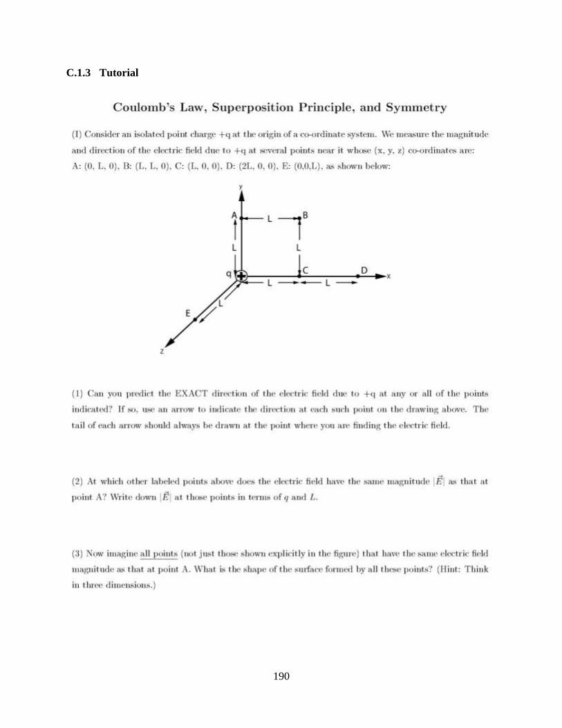
190

C.1.3 Tutorial

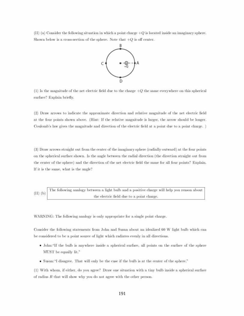
191

192

193

194

195

196

197

198

199

C.2 TUTORIAL II

C.2.1 Pre-test II

200

C.2.2 Post-test II

201

C.2.3 Tutorial II

202

203

204

205

APPENDIX D

TUTORIALS AND PRE-/POST-TESTS ON GAUSS’S LAW AND SUPERPOSITION

PRINCIPLE (CHAPTER 5)

D.1 TUTORIAL III

206

D.1.1 Pre-test III

207

D.1.2 Post-test III

208

D.1.3 Tutorial III

209

210

211

212

213

214

215

216

217

218

D.2 TUTORIAL IV

D.2.1 Pre-test IV

219

220

D.2.2 Post-test IV

221

222

D.2.3 Tutorial IV

223

224

225

226

227

228

229

230

231

232

D.3 TUTORIAL V

233

D.3.1 Pre-test V

234

D.3.2 Post-test V

235

236

D.3.3 Tutorial V

237

238

239

240

241

242

APPENDIX E

MAGNETISM CONCEPTUAL SURVEY (CHAPTER 6)

243

244

245

246

247

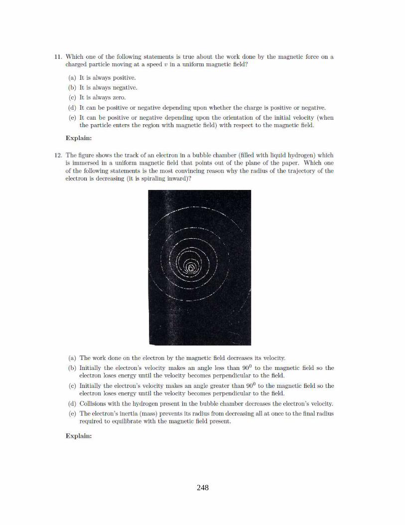
248

249

250

251

252

253

254

255

256

Documents

IMPROVING STUDENTS’ UNDERSTANDING OF … · Electricity and magnetism are important ... multiple choice questions and essay ... 4.5.11 Invoking the dynamics of charges in an electrostatics