IMPROVING SECOND ORDER REDUCED BIAS EXTREME … · IMPROVING SECOND ORDER REDUCED BIAS EXTREME VALUE INDEX ESTIMATION ... for all x>0. Equivalently, the quantile function U(t) = F

REVSTAT – Statistical Journal

Volume 5, Number 2, June 2007, 177–207

IMPROVING SECOND ORDER REDUCED BIAS

EXTREME VALUE INDEX ESTIMATION

Authors: M. Ivette Gomes– Universidade de Lisboa, D.E.I.O. and C.E.A.U.L., Portugal

[email protected]

M. Joao Martins– D.M., I.S.A., Universidade Tecnica de Lisboa, Portugal

[email protected]

Manuela Neves– D.M., I.S.A., Universidade Tecnica de Lisboa, Portugal

[email protected]

Received: November 2006 Accepted: February 2007

Abstract:

• Classical extreme value index estimators are known to be quite sensitive to the num-ber k of top order statistics used in the estimation. The recently developed secondorder reduced-bias estimators show much less sensitivity to changes in k. Here, weare interested in the improvement of the performance of reduced-bias extreme valueindex estimators based on an exponential second order regression model applied tothe scaled log-spacings of the top k order statistics. In order to achieve that improve-ment, the estimation of a “scale” and a “shape” second order parameters in the bias isperformed at a level k1 of a larger order than that of the level k at which we computethe extreme value index estimators. This enables us to keep the asymptotic varianceof the new estimators of a positive extreme value index γ equal to the asymptoticvariance of the Hill estimator, the maximum likelihood estimator of γ, under a strictPareto model. These new estimators are then alternatives to the classical estimators,not only around optimal and/or large levels k, but for other levels too. To enhance theinteresting performance of this type of estimators, we also consider the estimation ofthe “scale” second order parameter only, at the same level k used for the extreme valueindex estimation. The asymptotic distributional properties of the proposed class ofγ-estimators are derived and the estimators are compared with other similar alter-native estimators of γ recently introduced in the literature, not only asymptotically,but also for finite samples through Monte Carlo techniques. Case-studies in the fieldsof finance and insurance will illustrate the performance of the new second orderreduced-bias extreme value index estimators.

Key-Words:

• statistics of extremes; semi-parametric estimation; bias estimation; heavy tails; maxi-

mum likelihood.

AMS Subject Classification:

• 62G32, 62H12; 65C05.

178 M. Ivette Gomes, M. Joao Martins and Manuela Neves

Improving Second Order Reduced-Bias Extreme Value Index Estimation 179

1. INTRODUCTION AND MOTIVATION FOR THE NEWCLASSOF EXTREME VALUE INDEX ESTIMATORS

Examples of heavy-tailed models are quite common in the most diversified

fields. We may find them in computer science, telecommunication networks,

insurance, economics and finance, among other areas of application. In the area

of extreme value theory, a model F is said to be heavy-tailed whenever the tail

function, F := 1 − F , is a regularly varying function with a negative index of

regular variation equal to −1/γ, γ > 0, denoted F ∈ RV−1/γ , where the notation

RVα stands for the class of regularly varying functions at infinity with an index

of regular variation equal to α, i.e., positive measurable functions g such that

limt→∞ g(tx)/g(t) = xα, for all x > 0. Equivalently, the quantile function U(t) =

F←(1− 1/t), t ≥ 1, with F←(x) = inf{y : F (y) ≥ x}, is of regular variation with

index γ, i.e.,

(1.1) F is heavy-tailed ⇐⇒ F ∈ RV−1/γ ⇐⇒ U ∈ RVγ ,

for some γ > 0. Then, we are in the domain of attraction for maxima of an

extreme value distribution function (d.f.),

EVγ(x) =

{exp(−(1 + γx)−1/γ

), 1 + γx ≥ 0 if γ 6= 0 ,

exp(− exp(−x)

), x ∈ R if γ = 0 ,

but with γ > 0, and we write F ∈ DM(EVγ>0). The parameter γ is the extreme

value index, one of the primary parameters of extreme or even rare events.

The second order parameter ρ rules the rate of convergence in the first

order condition (1.1), let us say the rate of convergence towards zero of

lnU(tx) − lnU(t) − γ lnx, and is the non-positive parameter appearing in the

limiting relation

(1.2) limt→∞

lnU(tx) − lnU(t) − γ lnx

A(t)=

xρ − 1

ρ,

which we assume to hold for all x > 0, and where |A(t)| must then be of regular

variation with index ρ (Geluk and de Haan, 1987). We shall assume everywhere

that ρ < 0. The second order condition (1.2) has been widely accepted as an

appropriate condition to specify the tail of a Pareto-type distribution in a semi-

parametric way, and it holds for most common Pareto-type models.

Remark 1.1. For Hall–Welsh class of Pareto-type models (Hall and Welsh,

1985), i.e., models such that, with C > 0, D1 6= 0 and ρ < 0,

(1.3) U(t) = C tγ(1 +D1t

ρ + o(tρ)), as t→∞ ,

condition (1.2) holds and we may choose A(t) = ρD1 tρ.


Here, although not going into a general third order framework, as the one

found in Gomes et al. (2002) and Fraga Alves et al. (2003), in papers on the

estimation of ρ, as well as in Gomes et al. (2004a), in a paper on the estima-

tion of a positive extreme value index γ, we shall further specify the term o(tρ)

in Hall–Welsh class of models, and, for some particular details in the paper,

we shall assume to be working with a Pareto-type class of models with a quantile

function

(1.4) U(t) = C tγ(1 +D1t

ρ +D2 t2ρ + o(t2ρ)

),

as t→∞, with C > 0, D1, D2 6= 0, ρ< 0. Consequently, we may obviously choose,

in (1.2),

(1.5) A(t) = ρD1 tρ =: γ β tρ , β 6= 0, ρ < 0 ,

and, with

(1.6) B(t) = (2D2/D1−D1) tρ =: β′ tρ =

β′A(t)

β γ,

we may write

lnU(tx) − lnU(t) − γ lnx = A(t)

(xρ−1

ρ

)+A(t)B(t)

(x2ρ−1

2 ρ

)(1 + o(1)

).

The consideration of models in (1.4) enables us to get full information on the

asymptotic bias of the so-called second-order reduced-bias extreme value index

estimators, the type of estimators under consideration in this paper.

Remark 1.2. Most common heavy-tailed d.f.’s, like the Frechet, the Gen-

eralized Pareto (GP), the Burr and the Student’s t belong to the class of models

in (1.4), and consequently, to the class of models in (1.3) or, to the more general

class of parents satisfying (1.2).

For intermediate k, i.e., a sequence of integers k= kn, 1≤ k <n, such that

(1.7) k = kn → ∞ , kn = o(n), as n→∞ ,

and withXi:n denoting the i-th ascending order statistic (o.s.), 1≤ i≤ n, associated

to an independent, identically distributed (i.i.d.) random sample (X1, X2, ..., Xn),

we shall consider, as basic statistics, both the log-excesses over the random high

level lnXn−k:n, i.e.,

(1.8) Vik := lnXn−i+1:n − lnXn−k:n , 1≤ i≤ k <n ,

and the scaled log-spacings,

(1.9) Ui := i{lnXn−i+1:n − lnXn−i:n

}, 1≤ i≤ k <n .


We have a strong obvious link between the log-excesses and the scaled log-spacings

provided by the equation,∑k

i=1Vik =∑k

i=1 Ui.

It is well known that for intermediate k, and whenever we are working

with models in (1.1), the log-excesses Vik, 1≤ i ≤ k, are approximately the k

o.s.’s from an exponential sample of size k and mean value γ. Also, under the

same conditions, the scaled log-spacings Ui, 1≤ i ≤ k, are approximately i.i.d.

and exponential with mean value γ. Consequently, the Hill estimator of γ (Hill,

1975),

(1.10) H(k) ≡ Hn(k) =1

k

k∑

i=1

Vik =1

k

k∑

i=1

Ui ,

is consistent for the estimation of γ whenever (1.1) holds and k is intermediate,

i.e., (1.7) holds. Under the second order framework in (1.2) the asymptotic

distributional representation

(1.11) Hn(k)d= γ +

γ√kZ

(1)k +

A(n/k)

1− ρ

(1 + op(1)

)

holds, where Z(1)k =

√k(∑k

i=1Ei/k − 1), with {Ei} i.i.d. standard exponential

random variables (r.v.’s), is an asymptotically standard normal random variable.

Consequently,√k (Hn(k)− γ) converges weakly towards a normal r.v. with vari-

ance γ2 and a non-null mean value equal to λ/(1− ρ), whenever√k A(n/k) →

λ 6= 0, finite.

The adequate accommodation of the bias of Hill’s estimator has been

extensively addressed in recent years by several authors. Beirlant et al. (1999)

and Feuerverger and Hall (1999) consider exponential regression techniques,

based on the exponential approximations Ui ≈ γ(1 + b(n/k) (k/i)ρ

)Ei and

Ui ≈ γ exp(β (n/i)ρ

)Ei, respectively, 1 ≤ i ≤ k. They then proceed to the joint

maximum likelihood (ML) estimation of the three unknown parameters or func-

tionals at the same level k. Considering also the scaled log-spacings Ui in (1.9)

to be approximately exponential with mean value µi = γ exp(β(n/i)ρ

), 1≤ i≤ k,

β 6= 0, Gomes and Martins (2002) advance with the so-called “external” estima-

tion of the second order parameter ρ, i.e., an adequate estimation of ρ at a level k1

higher than the level k used for the extreme value index estimation, together with

a first order approximation for the ML estimator of β. They then obtain “quasi-

ML” explicit estimators of γ and β, both computed at the same level k, and

through that “external” estimation of ρ, are then able to reduce the asymptotic

variance of the extreme value index estimator proposed, comparatively to the

asymptotic variance of the extreme value index estimator in Feuerverger and

Hall (1999), where the three parameters γ, β and ρ are estimated at the same

level k. With the notation

(1.12) dk(α) =1

k

k∑

i=1

( ik

)α−1, Dk(α) =

1

k

k∑

i=1

( ik

)α−1Ui ,


for any real α ≥ 1 [Dk(1)≡H(k) in (1.10)], and with ρ any consistent estimator

of ρ, such estimators are

(1.13) γML

n (k) = H(k) − β(k; ρ)(nk

)ρDk(1− ρ)

and

(1.14) β(k; ρ) :=(kn

)ρ dk(1− ρ)×Dk(1) −Dk(1− ρ)

dk(1− ρ)×Dk(1− ρ) −Dk(1− 2 ρ),

for γ and β, respectively. This means that β, in (1.5), which is also a second

order parameter, is estimated at the same level k at which the γ-estimation

is performed, being β(k; ρ) — not consistent for the estimation of β whenever√k A(n/k) → λ, finite, but consistent for models in (1.2) and intermediate k

such that√k A(n/k) → ∞ (Gomes and Martins, 2002), — plugged in the extreme

value index estimator in (1.13). In all the above mentioned papers, authors have

been led to the now called “classical” second order reduced-bias extreme value

index estimators with an asymptotic variance larger or equal to γ2((1− ρ)/ρ

)2,

the minimal asymptotic variance of an asymptotically unbiased estimator in

Drees class of functionals (Drees, 1998).

We here propose an “external” estimation of both β and ρ, through β and ρ,

respectively, both using a number of top o.s.’s, k1, larger than the number of

top o.s.’s, k, used for the extreme value index estimation. We shall thus consider

the estimator

(1.15) MLβ,ρ(k) := H(k) − β(nk

)ρDk(1− ρ) ,

for adequate consistent estimators β and ρ of the second order parameters β and ρ,

respectively, to be specified in subsection 3.3 of this paper. Additionally, we shall

also deal with the estimator

(1.16) MLβ,ρ(k) =1

k

k∑

i=1

Ui exp(−β(n/i)ρ

),

the estimator directly derived from the likelihood equation for γ with β and ρ

fixed and based upon the exponential approximation, Ui ≈ γ exp(β(n/i)ρ

)Ei,

1 ≤ i ≤ k. Doing this, we are able to reduce the bias without increasing the

asymptotic variance, which is kept at the value γ2, the asymptotic variance of

Hill’s estimator. The estimators are thus better than the Hill estimator for all k.

Remark 1.3. If, in (1.15), we estimate β at the same level k used for

the estimation of γ, we may be led to γMLn (k) in (1.13). Indeed, γML

n (k) =

MLβ(k;ρ),ρ(k), with β(k; ρ) defined in (1.14).

Remark 1.4. The ML estimator in (1.15) may be obtained from the esti-

mator in (1.16) through the use of the first order approximation,{1− β(n/i)ρ

},

for the exponential weight, e−β(n/i)ρ, of the scaled log-spacing Ui, 1≤ i ≤ k.


Remark 1.5. The estimators in (1.15) and (1.16) have been inspired in

the recent papers of Gomes et al. (2004b) and Caeiro et al. (2005). These authors

consider, in different ways, the joint external estimation of both the “scale” and

the “shape” parameters in the A function in (1.2), parameterized as in (1.5), being

able to reduce the bias without increasing the asymptotic variance, which is kept

at the value γ2, the asymptotic variance of Hill’s estimator. Those estimators

are also going to be considered here for comparison with the new estimators in

(1.15) and (1.16). The reduced-bias extreme value index estimator in Gomes

et al. (2004b) is based on a linear combination of the log-excesses Vik in (1.8),

and is given by

(1.17) WHβ,ρ(k) :=1

k

k∑

i=1

e−β(n/k)ρ ψρ(i/k) Vik , ψρ(x) = −x−ρ − 1

ρ lnx,

with the notation WH standing for Weighted Hill estimator. Caeiro et al. (2005)

consider the estimator

(1.18) Hβ,ρ(k) := H(k)

(1− β

1− ρ

(nk

)ρ),

where the dominant component of the bias of Hill’s estimatorH(k) in (1.10), given

byA(n/k)/(1−ρ) = βγ(n/k)ρ/(1−ρ), is thus estimated throughH(k) β(n/k)ρ/(1−ρ),and directly removed from Hill’s classical extreme value index estimator.

As before, both in (1.17) and (1.18), β and ρ need to be adequate consistent

estimators of the second order parameters β and ρ, respectively, so that the

new estimators are better than the Hill estimator for all k.

In section 2 of this paper, and assuming first that only γ is unknown,

we shall state a theorem that provides an obvious technical motivation for the

estimators in (1.15) and (1.16). Next, in section 3, we consider the derivation of

the asymptotic behavior of the classes of estimators in (1.15) and (1.16), for an

appropriate estimation of β and ρ at a level k1 larger than the value k used for the

extreme value index estimation. We also do that only with the estimation of ρ,

estimating β at the same level k used for the extreme value index estimation.

In this same section, we finally briefly review the estimation of the two second

order parameters β and ρ. In section 4, using simulation techniques, we exhibit

the performance of the ML estimator in (1.15) and the ML estimator in (1.16),

comparatively to the other “Unbiased Hill” (UH ) estimators, WH and H, in

(1.17) and (1.18), respectively, to the classical Hill estimator H in (1.10) and to

the “asymptotically unbiased” estimator γMLn (k) in (1.13), studied in Gomes and

Martins (2002), or equivalently, MLβ(k;ρ),ρ, with MLβ,ρ the estimator in (1.15).

Section 5 is devoted to the illustration of the behavior of these estimators for

the Daily Log-Returns of the Euro against the UK Pound and automobile claims

gathered from several European insurance companies co-operating with the same

re-insurer (Secura Belgian Re).


2. ASYMPTOTIC BEHAVIOR OF THE ESTIMATORS (ONLY γ

IS UNKNOWN)

For real values α ≥ 1, and denoting again {Ei} a sequence of i.i.d. standard

exponential r.v.’s, let us introduce the following notation:

(2.1) Z(α)k =

√(2α−1)k

(1

k

k∑

i=1

( ik

)α−1Ei −

1

α

).

With the same kind of reasoning as in Gomes et al. (2005a), we state:

Lemma 2.1. Under the second order framework in (1.2), for intermediate

k-sequences, i.e., whenever (1.7) holds, and with Ui given in (1.9), we may guar-

antee that, for any real α ≥ 1, and Dk(α) given in (1.12),

Dk(α)d=

γ

α+

γ Z(α)k√

(2α− 1) k+A(n/k)

α− ρ

(1 + op(1)

),

where Z(α)k , given in (2.1), is an asymptotically standard normal random variable.

If we further assume to be working with models in (1.4), and with the same

notation as before, we may write for any α, β ≥ 1, α 6= β, the joint distribution

(Dk(α), Dk(β)

) d=(γα,γ

β

)+

γ√k

(Z

(α)k√

(2α− 1),

Z(β)k√

(2β − 1)

)

+ A(n/k)

(1

α−ρ,1

β−ρ

)+β′A2(n/k)

β γ

(1

α−2ρ,

1

β−2ρ

)(2.2)

+ Op

(A(n/k)√

k

)+ op

(A2(n/k)

),

with β and β′ given in (1.5) and (1.6), respectively.

Let us assume that only the extreme value index parameter γ is unknown,

and generally denote ML either ML or ML. This case obviously refers to a

situation which is rarely encountered in practice, but reveals the potential of

the classes of estimators in (1.15) and (1.16).

2.1. Known β and ρ

We may state:


Theorem 2.1. Under the second order framework in (1.2), further as-

suming that A(t) may be chosen as in (1.5), and for levels k such that (1.7)

holds, we get asymptotic distributional representations of the type

(2.3) MLβ,ρ(k)d= γ +

γ√kZ

(1)k + op

(A(n/k)

),

where Z(1)k is the asymptotically standard normal r.v. in (2.1) for α = 1.

Consequently,√k(MLβ,ρ(k) − γ

)is asymptotically normal with variance equal

to γ2, and with a null mean value not only when√k A(n/k) −→ 0, but also

when√k A(n/k) −→ λ 6= 0, finite, as n→ ∞.

For models in (1.4), we may further specify the term op(A(n/k)

), writing

MLβ,ρ(k)d= γ +

γ√kZ

(1)k +

(β′−β)A2(n/k)

β γ (1−2ρ)

(1+ op(1)

),(2.4)

MLβ,ρ(k)d= γ +

γ√kZ

(1)k +

(2β′−β)A2(n/k)

2β γ (1−2ρ)

(1+ op(1)

),(2.5)

with β and β′ given in (1.5) and (1.6), respectively. Consequently, even if√k A(n/k) → ∞, with

√k A2(n/k) → λ

A, finite,

√k (MLβ,ρ(k) − γ) and√

k (MLβ,ρ(k) − γ) are asymptotically normal with variance equal to γ2 and

asymptotic bias equal to

(2.6) bML

=(β′−β)λ

A

β γ (1−2ρ)and b

ML=

(2β′−β)λA

2β γ (1−2ρ),

respectively.

Proof: If all parameters are known, apart from the extreme value index γ,

we get directly from Lemma 2.1,

MLβ,ρ(k) := Dk(1) − β(nk

)ρDk(1−ρ)

d= γ +

γ√kZ

(1)k +

A(n/k)

1−ρ

− A(n/k)

γ

(γ

1−ρ +γ√

(1−2ρ)kZ

(1−ρ)k +

A(n/k)

1−2ρ

(1+ op(1)

))

d= γ +

γ√kZ

(1)k + op

(A(n/k)

).

Similarly, since we may write

MLβ,ρ(k) = MLβ,ρ(k) +A2(n/k)

2 γ2Dk(1−2ρ)

(1+ op(1)

)(2.7)

= MLβ,ρ(k) +A2(n/k)

2 γ (1−2ρ)

(1+ op(1)

),


(2.3) holds for ML as well. For models in (1.4), and directly from (2.2), we get

MLβ,ρ(k)d= γ +

γ√kZ

(1)k +

A(n/k)

1−ρ +β′A2(n/k)

β γ (1−2ρ)

(1+ op(1)

)+Op

(A(n/k)√

k

)

− A(n/k)

γ

(γ

1−ρ +γ√

(1−2ρ) kZ

(1−ρ)k +

A(n/k)

1− 2ρ

(1+ op(1)

)).

Working this expression, we finally obtain

MLβ,ρ(k)d= γ +

γ√kZ

(1)k +Op

(A(n/k)√

k

)+

A2(n/k)

γ(1−2ρ)

(β′

β− 1

)(1+ op(1)

),

i.e., (2.4) holds. Also directly from (2.4) and (2.7), (2.5) follows. Note that

since√k Op

(A(n/k)/

√k)

= Op(A(n/k)

)→ 0, the summand Op

(A(n/k)/

√k)

is

totally irrelevant for the asymptotic bias in (2.6), that follows straightforwardly

from the above obtained distributional representations.

Remark 2.1. We know that the asymptotic variances of ML and ML are

the same. Since λA≥ 0, b

ML= b

ML+ λ

A/(2 γ (1−2ρ)

)≥ b

ML. We may thus say

that, asymptotically, the ML-statistic is expected to exhibit a better performance

than ML, provided the bias are both positive. Things work the other way round

if the bias are both negative, i.e., the sample paths of ML are expected to be

in average above the ones of ML.

Remark 2.2. For the Burr d.f. F (x) = 1−(1+x−ρ/γ)1/ρ, x ≥ 0, we have

U(t) = tγ(1− tρ)−γ/ρ = tγ(1 + γ tρ/ρ + γ(γ+ρ) t2ρ/(2 ρ2) + o(t2ρ)

), for t ≥ 1.

Consequently, (1.4) holds with D1 = γ/ρ, D2 = γ(γ+ρ)/(2 ρ2), β′= β = 1 and

bML

= 0. A similar result holds for the GP d.f. F (x) = 1− (1+ γ x)−1/γ , x ≥ 0.

For this d.f., U(t) = (tγ−1)/γ, and (1.4) holds with ρ=−γ, D1 = −1 and D2 = 0.

Hence β = β′= 1 and bML

= 0. We thus expect a better performance of ML,

comparatively to ML, WH and H whenever the model underlying the data is

close to Burr or to GP models, a situation that happens often in practice, and

that is another point in favour of the ML-statistic.

2.2. Known ρ

We may state the following:

Theorem 2.2. For models in (1.4), if k= kn is a sequence of intermediate

integers, i.e., (1.7) holds, and if√k A(n/k) → ∞, with

√k A2(n/k) converging

towards λA, finite, as n→∞, then, with β(k; ρ), MLβ,ρ(k) and MLβ,ρ(k) given in

(1.14), (1.15) and (1.16), respectively, the asymptotic variance of both ML∗(k) =


MLβ(k;ρ),ρ(k) and ML∗(k) = MLβ(k;ρ),ρ(k) is equal to

(γ (1−ρ)/ρ

)2, being their

asymptotic bias given by

(2.8) b∗ML

=(β−β′) (1−ρ)λ

A

β γ (1−2ρ) (1−3ρ)and b∗

ML

=

(β (3−5ρ) − 2β′(1−ρ)

)λ

A

2β γ (1−2ρ) (1−3ρ),

respectively, again with β and β′ given in (1.5) and (1.6), respectively.

Proof: Following the steps in Gomes and Martins (2002), but working

now with models in (1.4) and the distributional representation (2.2), we may

write:

ML∗(k) = H(k) −Dk(1−ρ)

{Dk(1)

(1+ o(1)

)− (1−ρ)Dk(1−ρ)

}

Dk(1−ρ)(1+ o(1)

)− (1−ρ)Dk(1−2ρ)

=: H(k) − ϕk(ρ)

ψk(ρ),

with Dk(α) given in (1.12). Directly from (2.2), we get

1

ψk(ρ)= − (1−ρ) (1−2ρ)

γ ρ2

(1 −

{2(1−ρ)A(n/k)

γ (1−3ρ)+Op

(1√k

)}(1+ op(1)

))

and, under the conditions on k imposed,

ϕk(ρ) =γ2

√k

(Z

(1)k

1−ρ − Z(1−ρ)k√1− 2ρ

)− γ ρ2A(n/k)

(1−ρ)2 (1−2ρ)

− ρ2A2(n/k)

(1−ρ) (1−2ρ)

(2β′

β (1−3ρ)+

1

1− 2ρ

)(1+ op(1)

).

Consequently,

ϕk(ρ)

ψk(ρ)= − γ

ρ2√k

((1−2ρ)Z

(1)k − (1−ρ)

√1− 2ρ Z

(1−ρ)k

)+A(n/k)

1−ρ

+A2(n/k)

γ

(2(β′−β)

β (1− 3ρ)+

1

1− 2ρ

)(1+ op(1)

).

Then, with

Zk =

(1−ρρ

)2Z

(1)k −

((1−ρ)√1− 2ρ

ρ2

)Z

(1−ρ)k ,

ML∗(k) = MLβ(k;ρ),ρ(k)d= γ +

γ√kZk −

(β′−β) (1−ρ)A2(n/k)

β γ (1−2ρ) (1− 3ρ)

(1+ op(1)

),

and the result in (2.8) follows for ML∗(k). Also, since the asymptotic covariance

between Z(1)k and Z

(1−ρ)k is given by

√1− 2ρ /(1−ρ), the asymptotic variance of

Zk is given by

(1−ρρ

)4+

(1−ρ)2 (1−2ρ)

ρ4− 2(1−ρ)3 √1− 2ρ

ρ4×

√1− 2ρ

1−ρ =

(1−ρρ

)2.


Hence, the asymptotic variance γ2{(1−ρ)/ρ

}2, stated in the theorem. If we

consider MLβ(k;ρ),ρ(k), since√k A(n/k) → ∞, β(k; ρ) converges in probability

towards β and a result similar to (2.7) holds, i.e.,

ML∗(k) = MLβ(k;ρ),ρ(k) = MLβ(k;ρ),ρ(k) +

A2(n/k)

2γ (1−2ρ)

(1+ op(1)

).

The result in the theorem follows thus straightforwardly.

Remark 2.3. For models in (1.4) and λA6= 0 in Theorem 2.2, b∗

ML= 0 if

and only if β = β′. Again, this holds for Burr and GP underlying models.

Remark 2.4. When we look at Theorems 2.1 and 2.2, we see that, for

(β, ρ) known, despite the increasing in the asymptotic variance, (bML/b∗

ML)2 =(

(1−3ρ)/(1−ρ))2

is an increasing function of |ρ|, always greater than one,

for ρ < 0, i.e., there is here again a compromise between bias and variance.

2.3. Asymptotic comparison at optimal levels

We now proceed to an asymptotic comparison of ML and ML∗ at their

optimal levels in the lines of de Haan and Peng (1998), Gomes and Martins

(2001) and Gomes et al. (2005b, 2006), among others, but now for second order

reduced-bias estimators. Suppose γ•n(k) is a general semi-parametric estimator

of the extreme value index γ, for which the distributional representation

(2.9) γ•n(k)d= γ +

σ•√kZ•n + b•A

2(n/k) + op(A2(n/k)

)

holds for any intermediate k, and where Z•n is an asymptotically standard normal

random variable. Then we have

√k[γ•n(k)−γ

] d→ N(λAb•, σ

2•), as n→∞ ,

provided k is such that√k A2(n/k) → λ

A, finite, as n→ ∞. In this situation

we may write Bias∞[γ•n(k)] := b•A2(n/k) and Var∞[γ•n(k)] := σ2

•/k. The so-called

Asymptotic Mean Squared Error (AMSE ) is then given by

AMSE [γ•n(k)] :=σ2•

k+ b2•A

4(n/k) .

Using regular variation theory (Bingham et al., 1987), it may be proved that,

whenever b• 6= 0, there exists a function ϕ(n), dependent only on the underlying

model, and not on the estimator, such that

(2.10) limn→∞

ϕ(n)AMSE [γ•n0] = C(ρ) (σ2•)− 4ρ

1−4ρ (b2•)1

1−4ρ =: LMSE [γ•n0] ,


where γ•n0 := γ•n(k•0(n)), k•0(n) := arg infk AMSE [γ•n(k)], is the estimator γ•n(k)

computed at its optimal level, the level where its AMSE is minimum.

It is then sensible to consider the usual:

Definition 2.1. Given two second order reduced-bias estimators, γ(1)n (k)

and γ(2)n (k), for which distributional representations of the type (2.9) hold, with

constants (σ1, b1) and (σ2, b2), b1, b2 6= 0, respectively, both computed at their

optimal levels, the Asymptotic Root Efficiency (AREFF ) of γ(1)n0 relatively to

γ(2)n0 is AREFF1|2 ≡AREFFbγ(1)

n0 |bγ(2)n0

:=(LMSE

[γ

(2)n0

]/LMSE

[γ

(1)n0

])1/2, with LMSE

given in (2.10).

Remark 2.5. This measure was devised so that the higher the AREFF

measure the better the estimator 1 is, comparatively to the estimator 2.

Proposition 2.1. For every β 6= β′, if we compare ML = MLβ,ρ and

ML∗= MLβ(k;ρ),ρ, we get AREFFML|ML∗ = (1−ρ)2

((1− 3ρ) ρ−4ρ

)−1/(1−4ρ)> 1

for all ρ < 0.

We may also say that AREFFML|ML

> 1, for all ρ, β and β′. This indicator

depends then not only of ρ, but also of β and β′. This result, together with the

result in Proposition 2.1, provides again a clear indication on an overall better

performance of the ML estimator, comparatively to ML and ML∗.

3. EXTREME VALUE INDEX ESTIMATION BASED ON THE

ESTIMATION OF THE SECOND ORDER PARAMETERS

β AND ρ

Again for α ≥ 1, let us further introduce the following extra notations:

W(α)k = (2α−1)

√(2α−1) k/2

(1

k

k∑

i=1

( ik

)α−1ln( ik

)Ei +

1

α2

),(3.1)

D′k(α) =dDk(α)

dα:=

1

k

k∑

i=1

( ik

)α−1ln( ik

)Ui ,(3.2)

with Ui and Dk(α) given in (1.9) and (1.12), respectively.

Again with the same kind of reasoning as in Gomes et al. (2005a), we state:


Lemma 3.1. Under the second order framework in (1.2), for intermediate

k-sequences, i.e., whenever (1.7) holds, and with Ui given in (1.9), we may guar-

antee that, for any real α ≥ 1 and with D′k(α) given in (3.2),

(3.3) D′k(α)d= − γ

α2+

γ W(α)k

(2α−1)√

(2α−1) k/2− A(n/k)

(α−ρ)2(1+ op(1)

),

where W(α)k , in (3.1), are asymptotically standard normal r.v.’s.

3.1. Estimation of both second order parameters β and ρ at a lower

threshold

Let us assume first that we estimate both β and ρ externally at a level k1

of a larger order than the level k at which we compute the extreme value index

estimator, now assumed to be an intermediate level k such that√k A(n/k) → λ,

finite, as n→ ∞, with A(t) the function in (1.2). We may state the following:

Theorem 3.1. Under the initial conditions of Theorem 2.1, let us consider

the class of extreme value index estimators MLβ,ρ(k), with ML denoting again

either the ML estimator in (1.15) or the ML estimator in (1.16), with β and ρ

consistent for the estimation of β and ρ, respectively, and such that

(3.4) (ρ−ρ) lnn = op(1), as n→∞ .

Then,√k{MLβ,ρ(k)−γ

}is asymptotically normal with null mean value and vari-

ance σ21 = γ2, not only when

√k A(n/k) → 0, but also whenever

√k A(n/k) →

λ 6= 0, finite.

Proof: With the usual notation Xnp∼Yn if and only if Xn/Yn goes in

probability to 1, as n→ ∞, we may write

∂MLβ,ρ

∂β

p∼ −(nk

)ρDk(1−ρ) = −A(n/k) Dk(1−ρ)

β γ

p∼ − A(n/k)

β(1−ρ)and

∂MLβ,ρ

∂ρ

p∼ −A(n/k)

γ

(ln(nk

)Dk(1−ρ) −D′k(1−ρ)

)

p∼ −A(n/k)

1−ρ

(ln(nk

)+

1

1−ρ

).

If we estimate consistently ρ and β through the estimators β and ρ in the con-

ditions of the theorem, we may use Taylor’s expansion series, and we obtain

(3.5) MLβ,ρ(k)−MLβ,ρ(k)p∼ −A(n/k)

1−ρ

{(β−ββ

)+(ρ−ρ

)(ln(n/k)+

1

1−ρ

)}.


Consequently, taking into account the conditions in the theorem,

MLβ,ρ(k) − MLβ,ρ(k) = op(A(n/k)

).

Hence, if√k A(n/k) → λ, finite, Theorem 2.1 enables us to guarantee the results

in the theorem.

3.2. Estimation of the second order parameter ρ only at a lower

threshold

If we consider γ and β estimated at the same level k, we are going to have

an increase in the asymptotic variance of our final extreme value index estimators,

but we no longer need to assume that condition (3.4) holds. Indeed, as stated

in Corollary 2.1 of Theorem 2.1 in Gomes and Martins (2002), for the estimator

in (1.13), Theorem 3.2 in Gomes et al. (2004b), for the estimator WHβ(k;ρ),ρ and

Theorem 3.2 in Caeiro et al. (2005), for the estimator Hβ(k;ρ),ρ, we may state:

Theorem 3.2. (Gomes and Martins, 2002; Gomes et al., 2004b; Caeiro

et al., 2005) Under the second order framework in (1.2), if k = kn is a sequence

of intermediate integers, i.e., (1.7) holds, and if limn→∞

√k A(n/k) = λ, finite,

then, with UH denoting any of the statistics ML, ML, WH or H in (1.15),

(1.16), (1.17) and (1.18), respectively, ρ any consistent estimator of the second

order parameter ρ, and β(k; ρ) the β-estimator in (1.14),

(3.6)√k(UHβ(k;ρ),ρ(k) − γ

)d−→

n→∞Normal

(0, σ2

2 := γ2(1−ρ

ρ

)2),

i.e., the asymptotic variance of UHβ(k;ρ),ρ(k) increases of a factor((1−ρ)/ρ

)2> 1

for every ρ < 0.

Remark 3.1. If we compare Theorem 3.1 and Theorem 3.2, we see that,

as expected, the estimation of the two parameters γ and β at the same level k

induces an increase in the asymptotic variance of the final γ-estimator of a factor

given by((1−ρ)/ρ

)2, greater than 1. The estimation of the three parameters γ,

β and ρ at the same level k may still induce an extra increase in the asymptotic

variance of the final γ-estimator, as may be seen in Feuerverger and Hall (1999)

(where the three parameters are indeed computed at the same level k). These

authors get an asymptotic variance ruled by σ2FH

:= γ2((1−ρ)/ρ

)4, and we have

σ1 < σ2 < σFH

for all ρ < 0. Consequently, and taking into account asymptotic

variances, it seems convenient to estimate both β and ρ “externally”, at a level k1

of a larger order than the level k used for the estimation of the extreme value

index γ.


3.3. How to estimate the second order parameters

We now provide some details on the type of second order parameters’ es-

timators we think sensible to use in practice, together with their distributional

properties.

3.3.1. The estimation of ρ

Several classes of ρ-estimators are available in the literature. Among them,

we mention the ones introduced in Hall and Welsh (1985), Drees and Kaufman

(1998), Peng (1998), Gomes et al. (2002) and Fraga Alves et al. (2003). The one

working better in practice and for the most common heavy-tailed models, is the

one in Fraga Alves et al. (2003). We shall thus consider here particular members of

this class of estimators. Under adequate general conditions, and for ρ < 0, they

are semi-parametric asymptotically normal estimators of ρ, which show highly

stable sample paths as functions of k1, the number of top o.s.’s used, for a wide

range of large k1-values. Such a class of estimators has been first parameterized

by a tuning parameter τ > 0, but τ may be more generally considered as a real

number (Caeiro and Gomes, 2004), and is defined as

(3.7) ρ(k1; τ) ≡ ρτ (k1) ≡ ρ(τ)n (k1) := −

∣∣∣∣∣∣

3(T

(τ)n (k1) −1

)

T(τ)n (k1) − 3

∣∣∣∣∣∣,

where

T (τ)n (k1) :=

(M

(1)n (k1)

)τ −(M

(2)n (k1)/2

)τ/2(M

(2)n (k1)/2

)τ/2 −(M

(3)n (k1)/6

)τ/3 , τ ∈ R ,

with the notation abτ = b ln a, whenever τ = 0 and with

M (j)n (k) :=

1

k

k∑

i=1

{lnXn−i+1:n

Xn−k:n

}j, j ≥ 1

[M (1)n ≡H in (1.10)

].

We shall here summarize a particular case of the results proved in Fraga

Alves et al. (2003):

Proposition 3.1 (Fraga Alves et al., 2003). Under the second order frame-

work in (1.2), if k1 is an intermediate sequence of integers, and if√k1 A(n/k1) →

∞, as n→ ∞, the statistics ρ(τ)n (k1) in (3.7) converge in probability towards ρ,

as n→∞, for any real τ . Moreover, for models in (1.4), if we further assume


that√k1 A

2(n/k1) −→ λA1

, finite, ρτ (k1)≡ ρ(τ)n (k1) is asymptotically normal

with a bias proportional to λA1

, and{ρτ (k1) − ρ

}= Op

(1/(

√k1 A(n/k1))

).

If√k1A

2(n/k1) → ∞,{ρτ (k1)−ρ

}= Op

(A(n/k1)

).

Remark 3.2. Note that if we choose for the estimation of ρ a level k1

under the conditions that assure, in Proposition 3.1, asymptotic normality with

a non-null bias, we may guarantee that k1 = O(n−4ρ/(1−4ρ)

)and consequently√

k1 A(n/k1) = O(n−ρ/(1−4ρ)

). Hence, ρτ (k1) − ρ = Op

(1/(

√k1 A(n/k1))

)=

Op(nρ/(1−4ρ)

)= op(1/ lnn) provided that ρ < 0, i.e., (3.4) holds whenever

we assume ρ < 0.

Remark 3.3. The adaptive choice of the level k1 suggested in Remark 3.2

is not straightforward in practice. The theoretical and simulated results in Fraga

Alves et al. (2003), together with the use of these ρ-estimators in the Generalized

Jackknife statistics of Gomes et al. (2000), as done in Gomes and Martins (2002),

has led these authors to advise the choice k1 = min(n−1, [2n/ ln lnn]

), to esti-

mate ρ. Note however that with such a choice of k1,√k1A

2(n/k1) → ∞ and{ρτ (k1)−ρ

}= Op

(A(n/k1)

)= Op

((ln lnn)ρ

). Consequently, without any further

restrictions on the behavior of the ρ-estimators, we may no longer guarantee that

(3.4) holds.

Remark 3.4. Here, and inspired in the results in Gomes et al. (2004b)

for the estimator in (1.17), we advise the consideration of a level of the type

(3.8) k1 =[n1−ǫ

], for some ǫ > 0, small ,

where [x] denotes, as usual, the integer part of x. When we consider the level k1

in (3.8),√k1 A

2(n/k1) → ∞, if and only if ρ > 14 − 1

4ǫ → −∞, as ǫ→ 0, and

such a condition is an almost irrelevant restriction in the underlying model,

provided we choose a small value of ǫ. For instance, if we choose ǫ = 0.001,

we get ρ > −249.75. Then, and with such an irrelevant restriction in the models

in (1.4), if we work with any of the ρ-estimators in this section, computed at the

level k1, {ρ−ρ} is of the order of A(n/k1) = O(nǫ×ρ), which is of smaller order

than 1/ lnn. This means that, again, condition (3.4) holds, being the choice in

(3.8) a very adequate choice in practice.

We advise practitioners not to choose blindly the value of τ in (3.7). It is

sensible to draw some sample paths of ρ(k; τ), as functions of k and for a few

τ -values, electing the value of τ ≡ τ∗ which provides the highest stability for

large k, by means of any stability criterion, like the ones suggested in Gomes

et al. (2004a), Gomes and Pestana (2004) and Gomes et al. (2005a). Anyway,

in all the Monte Carlo simulations we have considered the level k1 in (3.8), with


ǫ = 0.001, and

(3.9) ρτ := −

∣∣∣∣∣∣

3(T

(τ)n (k1) − 1

)

T(τ)n (k1) − 3

∣∣∣∣∣∣, τ =

{0 if ρ≥−1 ,

1 if ρ<−1 .

Indeed, an adequate stability criterion, like the one used in Gomes and Pestana

(2004), has practically led us to this choice for all models simulated, whenever the

sample size n is not too small. Note also that the choice of the most adequate

value of τ , let us say the tuning parameter τ = τ∗ mentioned before, is much

more relevant than the choice of the level k1, in the ρ-estimation and everywhere

in the paper, whenever we use second order parameters’ estimators in order to

estimate the extreme value index.

From now on we shall generally use the notation ρ ≡ ρτ = ρ(k1; τ) for any

of the estimators in (3.7) computed at a level k1 in (3.8).

3.3.2. The estimation of β based on the scaled log-spacings

We have here considered the estimator of β obtained in Gomes and Martins

(2002), already defined in (1.14), and based on the scaled log-spacings Ui in (1.9),

1≤ i ≤ k. The first part of the following result has been proved in Gomes and

Martins (2002) and the second part, related to the behavior of β(k; ρ(k; τ)), has

been proved in Gomes et al. (2004b):

Proposition 3.2 (Gomes and Martins, 2002; Gomes et al., 2004b). If the

second order condition (1.2) holds, with A(t) = β γ tρ, ρ < 0, if k = kn is

a sequence of intermediate positive integers, i.e. (1.7) holds, and if limn→∞√k A(n/k) =∞, then β(k;ρ), defined in (1.14), converges in probability towards β,

as n→∞. Moreover, if (3.4) holds, β(k;ρ) is consistent for the estimation of β.

We may further say that

(3.10) β(k; ρ(k; τ)

)− β

p∼ −β ln(n/k)(ρ(k; τ)−ρ

),

with ρ(k;τ) given in (3.7). Consequently, β(k; ρ(k;τ)

)is consistent for the estima-

tion of β whenever (1.7) holds and√k A(n/k)/ ln(n/k) → ∞. For models in (1.4),

β(k; ρ(k;τ)

)− β = Op

(ln(n/k)/(

√k A(n/k))

)whenever

√k A2(n/k) → λ

A, finite.

If√k A2(n/k) → ∞, then β

(k; ρ(k; τ)

)− β = Op

(ln(n/k) A(n/k)

).

An algorithm for second order parameter estimation, in a context of high

quantiles estimation, can be found in Gomes and Pestana (2005).


4. FINITE SAMPLE BEHAVIOR OF THE ESTIMATORS

4.1. Simulated models

In the simulations we have considered the following underlying parents:

the Frechet model, with d.f. F (x) = exp(−x−1/γ), x ≥ 0, γ > 0, for which

ρ=−1, β =1/2, β′= 5/6; and the GP model, with d.f. F (x) = 1− (1+γ x)−1/γ ,

x ≥ 0, γ > 0, for which ρ = −γ, β =1, β′= 1.

4.2. Mean values and mean squared error patterns

We have here implemented simulation experiments with 5000 runs, based on

the estimation of β at the level k1 in (3.8), with ǫ = 0.001, the same level we have

used for the estimation of ρ. We use the notation βj1 = β(k1; ρj), j = 0, 1, with

β(k; ρ) and ρτ , τ = 0, 1, given in (1.14) and (3.9), respectively. Similarly to what

has been done in Gomes et al. (2004b) for the WH -estimator, in (1.17), and in

Caeiro et al. (2005) for theH-estimator, in (1.18), these estimators of ρ and β have

been also incorporated in the ML-estimators, leading to ML0(k) ≡ MLβ01,ρ0(k)

or to ML1(k) ≡ MLβ11,ρ1(k), with ML denoting both ML and ML in (1.15) and

(1.16), respectively.

The simulations show that the extreme value index estimators UHj(k) ≡UHβj1,ρj

(k), with UH denoting again either ML or ML or WH or H, j equal

to either 0 or 1, according as |ρ| ≤ 1 or |ρ| > 1, seem to work reasonably well,

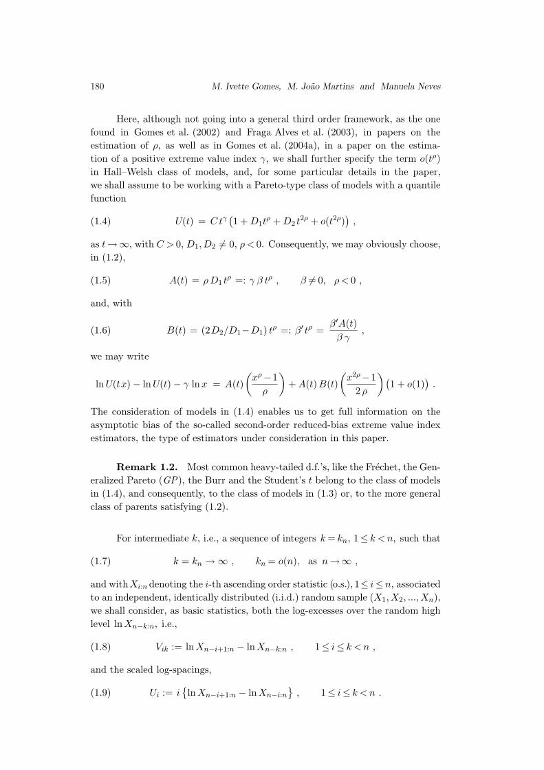
as illustrated in Figures 1, 2 and 3. In these figures we picture for the above

mentioned underlying models, and a sample of size n= 1000, the mean values

(E[•]) and the mean squared errors (MSE [•]) of the Hill estimator H, together

with UHj (left), UH ∗j ≡ UHβ(k;ρj),ρj(right), with j = 0 or j = 1, according as

|ρ| ≤ 1 or |ρ|> 1 and the r.v.’s UH ≡ UH β,ρ (center). The discrepancy, in some

of the models, between the behavior of the estimators proposed in this paper,

the ones in the left figures, and the r.v.’s, in the central ones, suggests that

some improvement in the estimation of second order parameters β and ρ is still

welcome.

Remark 4.1. For the Frechet model (Figure 1), the UHβ,ρ estimators

exhibit a negative bias up to moderate values of k and consequently, as hinted

in Remark 2.1, the ML statistic is the one exhibiting the worst performance in

terms of bias and minimum mean squared error. The ML0 estimator, always quite

close to WH0, exhibits the best performance among the statistics considered.


Figure 1: Underlying Frechet parent with γ = 1 (ρ=−1).

Figure 2: Underlying GP parent with γ = 0.5 (ρ=−0.5).


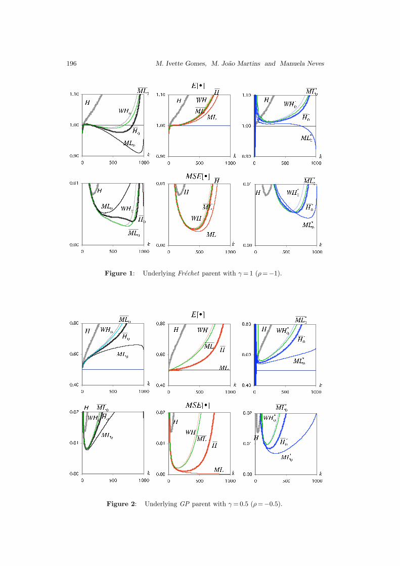
Figure 3: Underlying GP parent with γ = 2 (ρ=−2).

Things work the other way round, either with the r.v.’s UH (Figure 1, center) or

with the statistics UH ∗0 (Figure 1, right). The ML∗0 statistic is then the one with

the best performance.

Remark 4.2. For a GP model, we make the following comments:

1) The ML statistic behaves indeed as a “really unbiased” estimator of γ,

should we get to know the true values of β and ρ (see the central graphs

of Figures 2 and 3). Indeed bML

= 0 (see Remark 2.2), but we believe

that more than this happens, although we have no formal proof of the

unbiasedness of ML(k) for all k and for Burr and GP models, among

other possible parents.

2) For values of ρ>−1 (Figure 2), the estimators exhibit a positive bias,

overestimating the true value of the parameter, and the ML-statistic

is better than H, which on its turn behaves better than ML, this one

better than WH , both regarding bias and mean squared error and

in all situations (either when β and ρ are known or when β and ρ

are estimated at the larger level k1 or when only ρ is estimated at a

larger level k1, with β estimated at the same level than the extreme

value index).


3) For ρ <−1 (Figure 3), we need to use ρ1 (instead of ρ0) or an hybrid

estimator like the one suggested in Gomes and Pestana (2004).

In all the simulated cases the ML1-statistic is always the best one,

being ML1, H1 and WH1 almost equivalent.

4.3. Simulated comparative behavior at optimal levels

In Table 1, for the above mentioned Frechet(γ = 1), GP (γ = .5) and

GP (γ = 2) parents and for the r.v.’s UH ≡ UH β,ρ, we present the simulated val-

ues of the following characteristics at optimal levels: the optimal sample sample

fraction (OSF )/ mean value (E) (first row) and the mean squared error (MSE )/

Relative Efficiency (REFF ) indicator (second row). The simulated output is

now based on a multi-sample simulation of size 1000×10, and standard errors,

although not shown, are available from the authors. The OSF is, for any Tn(k),

OSFT≡ k

(T )0 (n)

n:=

arg mink MSE(Tn(k)

)

n,

and, relatively to the Hill estimator Hn(k) in (1.10), the REFF indicator is

REFFT

:=

√MSE

[Hn

(k

(H)0 (n)

)]/MSE

[Tn(k

(T )0 (n)

)].

For any value of n, and among the four r.v.’s, the largest REFF (equivalent to

smallest MSE ) is in bold and underlined.

It is clear from Table 1 the overall best performance of ML estimator,

whenever (β, ρ) is assumed to be known. Indeed, since bML

= 0, we were intuitively

expecting this type of performance. The choice is not so clear-cut when we

consider the estimation of the second order parameters, and either the statistics

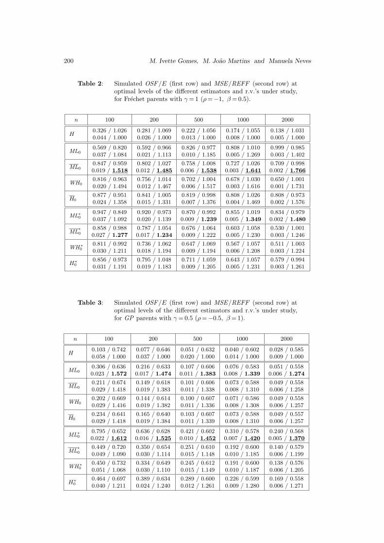
UHj or the statistics UH ∗j . Tables 2, 3 and 4 are similar to Table 1, but for the

extreme value index estimators UHj and UH ∗j , j = 0 or 1 according as |ρ| ≤ 1 or

|ρ > 1. Again, for any value of n, and among any four estimators of the same type,

the largest REFF (equivalent to smallest MSE ) is also in bold and underlined

if it attains the largest value among all estimators, or only in bold if it attains

the largest value among estimators of the same type.

A few remarks:

• For Frechet parents, and among the UH ∗0 estimators, the best perfor-

mance is associated to ML∗0 for n < 500 and to ML∗0 for n ≥ 500. Among

the UH0 estimators, ML0 exhibits the best performance for all n.


• For GP parents with γ = 0.5, ML0 exhibits the best performance among

the UH0 statistics. ML∗0 is also the best among the UH ∗0 statistics,

behaving ML∗0 better than ML0, for all n.

• For GP parents with γ = 2, ML1 exhibits the best performance among

the UH1 statistics. ML∗1 is also the best among the UH ∗1 statistics.

Now, ML∗1 behaves better than ML1, for n ≥ 500 and for n < 500

ML1 performs better than ML∗1.

Table 1: Simulated OSF/E (first row) and MSE/REFF (second row)at optimal levels of the r.v.’s under study.

n 100 200 500 1000 2000

Frechet parent, γ = 1 (ρ = −1)

ML0.642 / 0.986 0.599 / 1.017 0.517 / 1.037 0.473 / 1.039 0.429 / 1.0120.015 / 1.678 0.009 / 1.734 0.004 / 1.832 0.002 / 1.909 0.001 / 2.001

ML0.608 / 0.971 0.544 / 1.008 0.477 / 1.045 0.416 / 1.040 0.367 / 1.0070.016 / 1.647 0.010 / 1.662 0.005 / 1.727 0.003 / 1.782 0.002 / 1.855

WH0.580 / 0.960 0.513 / 1.019 0.450 / 1.052 0.395 / 1.041 0.357 / 1.0030.018 / 1.539 0.011 / 1.577 0.005 / 1.658 0.003 / 1.723 0.002 / 1.805

H0.587 / 0.963 0.537 / 1.012 0.482 / 1.048 0.436 / 1.041 0.379 / 1.0080.018 / 1.560 0.010 / 1.609 0.005 / 1.710 0.003 / 1.786 0.001 / 1.874

GP parent, γ = 0.5 (ρ = −0.5)

ML0.987 / 0.507 0.985 / 0.513 0.991 / 0.504 0.990 / 0.504 0.997 / 0.5030.002 / 5.813 0.001 / 6.567 0.000 / 7.831 0.000 / 9.184 0.000 / 10.487

ML0.295 / 0.565 0.240 / 0.545 0.183 / 0.530 0.157 / 0.531 0.124 / 0.5230.009 / 2.529 0.006 / 2.561 0.003 / 2.591 0.002 / 2.697 0.001 / 2.753

WH0.273 / 0.573 0.221 / 0.566 0.174 / 0.537 0.146 / 0.533 0.117 / 0.5300.012 / 2.246 0.007 / 2.332 0.004 / 2.419 0.002 / 2.542 0.001 / 2.624

H0.391 / 0.549 0.353 / 0.537 0.302 / 0.536 0.262 / 0.5200 0.208 / 0.5210.007 / 2.918 0.004 / 3.128 0.002 / 3.367 0.001 / 3.597 0.001 / 3.835

GP parent, γ = 2 (ρ = −2)

ML0.990 / 2.065 0.994 / 1.921 0.995 / 1.992 0.993 / 2.011 0.999 / 2.0150.032 / 1.923 0.016 / 2.030 0.006 / 2.211 0.00 / 2.382 0.002 / 2.541

ML0.731 / 2.111 0.677 / 1.956 0.633 / 2.033 0.588 / 2.047 0.549 / 2.0630.050 / 1.530 0.027 / 1.544 0.012 / 1.573 0.007 / 1.602 0.004 / 1.640

WH0.659 / 2.091 0.633 / 1.977 0.576 / 2.036 0.540 / 2.057 0.505 / 2.0620.058 / 1.420 0.031 / 1.450 0.014 / 1.496 0.008 / 1.528 0.004 / 1.573

H0.669 / 2.103 0.647 / 1.976 0.604 / 2.047 0.574 / 2.053 0.533 / 2.0570.058 / 1.423 0.030 / 1.470 0.013 / 1.525 0.007 / 1.570 0.004 / 1.622


Table 2: Simulated OSF/E (first row) and MSE/REFF (second row) atoptimal levels of the different estimators and r.v.’s under study,for Frechet parents with γ = 1 (ρ=−1, β= 0.5).

n 100 200 500 1000 2000

H0.326 / 1.026 0.281 / 1.069 0.222 / 1.056 0.174 / 1.055 0.138 / 1.0310.044 / 1.000 0.026 / 1.000 0.013 / 1.000 0.008 / 1.000 0.005 / 1.000

ML00.569 / 0.820 0.592 / 0.966 0.826 / 0.977 0.808 / 1.010 0.999 / 0.9850.037 / 1.084 0.021 / 1.113 0.010 / 1.185 0.005 / 1.269 0.003 / 1.402

ML00.847 / 0.959 0.802 / 1.027 0.758 / 1.008 0.727 / 1.026 0.709 / 0.9980.019 / 1.518 0.012 / 1.485 0.006 / 1.538 0.003 / 1.641 0.002 / 1.766

WH00.816 / 0.963 0.756 / 1.014 0.702 / 1.004 0.678 / 1.030 0.650 / 1.0010.020 / 1.494 0.012 / 1.467 0.006 / 1.517 0.003 / 1.616 0.001 / 1.731

H00.877 / 0.951 0.841 / 1.005 0.819 / 0.998 0.808 / 1.026 0.808 / 0.9730.024 / 1.358 0.015 / 1.331 0.007 / 1.376 0.004 / 1.469 0.002 / 1.576

ML∗

00.947 / 0.849 0.920 / 0.973 0.870 / 0.992 0.855 / 1.019 0.834 / 0.9790.037 / 1.092 0.020 / 1.139 0.009 / 1.239 0.005 / 1.349 0.002 / 1.480

ML∗

00.858 / 0.988 0.787 / 1.054 0.676 / 1.064 0.603 / 1.058 0.530 / 1.0010.027 / 1.277 0.017 / 1.234 0.009 / 1.222 0.005 / 1.230 0.003 / 1.246

WH∗

00.811 / 0.992 0.736 / 1.062 0.647 / 1.069 0.567 / 1.057 0.511 / 1.0030.030 / 1.211 0.018 / 1.194 0.009 / 1.194 0.006 / 1.208 0.003 / 1.224

H∗

00.856 / 0.973 0.795 / 1.048 0.711 / 1.059 0.643 / 1.057 0.579 / 0.9940.031 / 1.191 0.019 / 1.183 0.009 / 1.205 0.005 / 1.231 0.003 / 1.261

Table 3: Simulated OSF/E (first row) and MSE/REFF (second row) atoptimal levels of the different estimators and r.v.’s under study,for GP parents with γ = 0.5 (ρ=−0.5, β= 1).

n 100 200 500 1000 2000

H0.103 / 0.742 0.077 / 0.646 0.051 / 0.632 0.040 / 0.602 0.028 / 0.5850.058 / 1.000 0.037 / 1.000 0.020 / 1.000 0.014 / 1.000 0.009 / 1.000

ML00.306 / 0.636 0.216 / 0.633 0.107 / 0.606 0.076 / 0.583 0.051 / 0.5580.023 / 1.572 0.017 / 1.474 0.011 / 1.383 0.008 / 1.339 0.006 / 1.274

ML00.211 / 0.674 0.149 / 0.618 0.101 / 0.606 0.073 / 0.588 0.049 / 0.5580.029 / 1.418 0.019 / 1.383 0.011 / 1.338 0.008 / 1.310 0.006 / 1.258

WH00.202 / 0.669 0.144 / 0.614 0.100 / 0.607 0.071 / 0.586 0.049 / 0.5580.029 / 1.416 0.019 / 1.382 0.011 / 1.336 0.008 / 1.308 0.006 / 1.257

H00.234 / 0.641 0.165 / 0.640 0.103 / 0.607 0.073 / 0.588 0.049 / 0.5570.029 / 1.418 0.019 / 1.384 0.011 / 1.339 0.008 / 1.310 0.006 / 1.257

ML∗

00.795 / 0.652 0.636 / 0.628 0.421 / 0.602 0.310 / 0.578 0.240 / 0.5680.022 / 1.612 0.016 / 1.525 0.010 / 1.452 0.007 / 1.420 0.005 / 1.370

ML∗

00.449 / 0.720 0.350 / 0.654 0.251 / 0.610 0.192 / 0.600 0.140 / 0.5790.049 / 1.090 0.030 / 1.114 0.015 / 1.148 0.010 / 1.185 0.006 / 1.199

WH∗

00.450 / 0.732 0.334 / 0.649 0.245 / 0.612 0.191 / 0.600 0.138 / 0.5760.051 / 1.068 0.030 / 1.110 0.015 / 1.149 0.010 / 1.187 0.006 / 1.205

H∗

00.464 / 0.697 0.389 / 0.634 0.289 / 0.600 0.226 / 0.599 0.169 / 0.5580.040 / 1.211 0.024 / 1.240 0.012 / 1.261 0.009 / 1.280 0.006 / 1.271


Table 4: Simulated OSF/E (first row) and MSE/REFF (second row) atoptimal levels of the different estimators and r.v.’s under study,for GP parents with γ = 2 (ρ=−2, β= 1).

n 100 200 500 1000 2000

H0.415 / 2.179 0.359 / 1.968 0.319 / 2.018 0.290 / 2.068 0.251 / 2.0690.117 / 1.000 0.064 / 1.000 0.030 / 1.000 0.018 / 1.000 0.010 / 1.000

ML10.817 / 2.184 0.647 / 2.012 0.663 / 2.048 0.657 / 2.077 1.000 / 2.0940.071 / 1.282 0.043 / 1.221 0.021 / 1.194 0.013 / 1.173 0.007 / 1.180

ML10.631 / 2.140 0.558 / 2.008 0.478 / 2.044 0.399 / 2.050 0.358 / 2.0400.079 / 1.215 0.046 / 1.184 0.022 / 1.168 0.013 / 1.158 0.008 / 1.153

WH10.623 / 2.155 0.554 / 2.024 0.470 / 2.048 0.396 / 2.051 0.349 / 2.0410.081 / 1.197 0.047 / 1.171 0.023 / 1.159 0.013 / 1.153 0.008 / 1.149

H10.618 / 2.167 0.545 / 2.041 0.470 / 2.050 0.396 / 2.051 0.349 / 2.0410.083 / 1.186 0.047 / 1.165 0.023 / 1.156 0.013 / 1.152 0.008 / 1.148

ML∗

10.990 / 2.194 0.935 / 2.000 0.828 / 2.034 0.768 / 2.077 0.681 / 2.0550.072 / 1.272 0.044 / 1.211 0.021 / 1.204 0.012 / 1.197 0.007 / 1.191

ML∗

10.751 / 2.199 0.696 / 1.993 0.624 / 2.044 0.571 / 2.065 0.519 / 2.0410.089 / 1.143 0.050 / 1.129 0.024 / 1.123 0.014 / 1.125 0.008 / 1.130

WH∗

10.711 / 2.240 0.652 / 2.002 0.595 / 2.038 0.548 / 2.070 0.510 / 2.0450.100 / 1.079 0.054 / 1.087 0.025 / 1.098 0.014 / 1.105 0.008 / 1.115

H∗

10.710 / 2.240 0.657 / 2.001 0.604 / 2.041 0.561 / 2.071 0.513 / 2.0410.10 / 1.0780 0.054 / 1.088 0.025 / 1.101 0.014 / 1.109 0.008 / 1.120

4.4. An overall conclusion

The main advantage of the estimators UHj , and particularly of the MLj

estimators in this paper, the ones with an overall better performance, lies on

the fact that we may estimate β and ρ adequately through β and ρ so that the

MSE of the new estimator is smaller than the MSE of Hill’s estimator for all k,

even when |ρ|> 1, a region where it has been difficult to find alternatives for the

Hill estimator. And this happens together with a higher stability of the sample

paths around the target value γ. These new estimators work indeed better than

the Hill estimator for all values of k, contrarily to the alternatives so far available

in the literature, like the alternatives UH ∗j , j = 0 or 1, also considered in this

paper for comparison.


5. CASE-STUDIES IN THE FIELDS OF FINANCE AND

INSURANCE

5.1. Euro-UK Pound daily exchange rates

We shall first consider the performance of the above mentioned estimators

in the analysis of the Euro-UK Pound daily exchange rates from January 4, 1999

until December 14, 2004. This data has been collected by the European System of

Central Banks, and was obtained from http://www.bportugal.pt/rates/cambtx/.

In Figure 4 we picture the Daily Exchange Rates xt over the above mentioned

period and the Log-Returns, rt = 100×(lnxt − lnxt−1), the data to be analyzed.

Indeed, although conscious that the log-returns of any financial time-series are not

i.i.d., we also know that the semi-parametric behavior of estimators of rare event

parameters may be generalized to weak dependent data (see Drees, 2002, and

references therein). Semi-parametric estimators of extreme events’ parameters,

devised for i.i.d. processes, are usually based on the tail empirical process, and

remain consistent and asymptotically normal in a large class of weakly dependent

data.

Figure 4: Daily Exchange Rates (left) and Daily Log-Returns (right)on Euro-UK Pound Exchange Rate.

The histogram in Figure 5 points to a heavy right tail. Indeed, the empirical

counterparts of the usual skewness and kurtosis coefficients are β1 = 0.424 and

β2 = 1.835, clearly greater than 0, the target value for an underlying normal

parent.

In Figure 6, and working with the n0 = 725 positive log-returns, we now

picture the sample paths of ρ(k; τ) in (3.7) for τ = 0, and 1 (left), as functions

of k. The sample paths of the ρ-estimates associated to τ = 0 and τ = 1 lead us


Figure 5: Histogram of the Daily Log-Returns on the Euro-UK Pound.

to choose, on the basis of any stability criterion for large values of k, the esti-

mate associated to τ = 0. In Figure 6 we thus present the associated second order

parameters estimates, ρ0 = ρ0(721) = −0.65 (left) and β0 = βρ0(721) = 1.03,

together with the sample paths of β(k; ρ0) in (1.14), for τ = 0 (center). The sam-

ple paths of the classical Hill estimator in (1.10) (H) and of three of reduced-bias,

second order extreme value index estimates discussed in this paper, associated

to ρ0 = −0.65 and β0 = 1.03, are also pictured in Figure 6 (right). We do not

picture the statistic WH0 because that statistic practically overlaps ML0.

Figure 6: Estimates of the second order parameter ρ (left), of the secondorder parameter β (center) and of the extreme value index (right),for the Daily Log-Returns on the Euro-UK Pound.

The Hill estimator exhibits a relevant bias, as may be seen from Figure 6,

and we are for sure a long way from the strict Pareto model. The other estimators,

ML0, ML0 and H0, which are “asymptotically unbiased”, reveal without doubt


a bias much smaller than that of the Hill. All these statistics enable us to take

a decision upon the estimate of γ to be used, with the help of any stability crite-

rion, but the ML statistic is without doubt the one with smallest bias, among the

statistics considered. More important than this: we know that any estimate con-

sidered on the basis of ML0(k) (or any of the other three reduced-bias statistics)

performs for sure better than the estimate based on H(k) for any level k. Here,

we represent the estimate γ ≡ γML

= 0.30, the median of the ML estimates, for

thresholds k between[n−2ρ/(1−2ρ)0 /4

]= 10 and

[4×n−2ρ/(1−2ρ)

0

]= 165, chosen in

an heuristic way. If we use this same criterion on the estimates ML, WH and H

we are also led to the same estimate, γML

≡ γWH

≡ γH

= 0.30. The development

of adequate techniques for the adaptive choice of the optimal threshold for

this type of second order reduced-bias extreme value index estimators is needed,

being indeed an interesting topic of research, but is outside the scope of the

present paper.

5.2. Automobile claims

We shall next consider an illustration of the performance of the above men-

tioned estimators, through the analysis of automobile claim amounts exceeding

1,200.000 Euros, over the period 1988–2001, and gathered from several European

insurance companies co-operating with the same re-insurer (Secura Belgian Re).

This data set has already been studied, for instance, in Beirlant et al. (2004).

Figure 7 is similar to Figure 5, but for the Secura data. It is now quite clear

the heaviness of the right tail. The empirical skewness and kurtosis coefficients

are β1 = 2.441 and β2 = 8.303. Here, the existence of left-censoring is also clear,

begin the main reason for the high skewness and kurtosis values.

Figure 7: Histogram or the Secura data.


Finally, in Figure 8, working with the n= 371 automobile claims exceeding

1,200.000 Euro, we present the sample path of the ρτ (left), ρτ (center) estimates,

as function of k, for τ = 0 and τ = 1, together with the sample paths of estimates

of the extreme value index γ, provided by the Hill estimator, H, the M -estimator

and the M estimator (right).

-3.00

-2.50

-2.00

-1.50

-1.00

-0.50

0.00

100 200 300 400

0.0

0.5

1.0

1.5

100 200 300 400

0.1

0.2

0.3

0.4

0.5

0 100 200 300 400

"0(k)

" = #0.65

"0(k)

" = 0.78

k

k

" = 0.23

H

k

ML0

H0

ML0

Figure 8: Estimates of the second order parameter ρ (left) and of theextreme value index γ (right) for the automobile claims.

Again, the ML0 statistic is the one exhibiting the best performance, leading

us to the estimate γ = 0.23.

ACKNOWLEDGMENTS

Research partially supported by FCT/POCTI and POCI/FEDER.

REFERENCES

[1] Bingham, N.H.; Goldie, C.M. and Teugels, J.L. (1987). Regular Variation,Cambridge University Press.

[2] Beirlant, J.; Dierckx, G.; Goegebeur, Y. and Matthys, G. (1999). Tailindex estimation and an exponential regression model, Extremes, 2, 177–200.

[3] Beirlant, J.; Goegebeur, Y.; Segers, J. and Teugels, J. Statistics of

Extremes. Theory and Applications, Wiley, New York.

[4] Caeiro, F. and Gomes, M.I. (2004). A new class of estimators of the “scale”second order parameter. To appear in Extremes.


[5] Caeiro, F.; Gomes, M.I. and Pestana, D.D. (2005). Direct reduction of biasof the classical Hill estimator, Revstat, 3, 2, 113–136.

[6] Drees, H. (1998). A general class of estimators of the tail index, J. Statist.

Planning and Inference, 98, 95–112.

[7] Drees, H. (2002). Tail empirical processes under mixing conditions. In “Empir-ical Process Techniques for Dependent Data” (Dehling et al., Eds.), Birkhauser,Boston, 325–342.

[8] Drees, H. and Kaufmann, E. (1998). Selecting the optimal sample fraction inunivariate extreme value estimation, Stoch. Proc. and Appl., 75, 149–172.

[9] Feuerverger, A. and Hall, P. (1999). Estimating a tail exponent by mod-elling departure from a Pareto distribution, Ann. Statist., 27, 760–781.

[10] Fraga Alves, M.I.; Gomes, M.I. and de Haan, L. (2003). A new class ofsemi-parametric estimators of the second order parameter, Portugaliae Mathe-

matica, 60, 1, 193–213.

[11] Geluk, J. and de Haan, L. (1987). Regular Variation, Extensions and Taube-

rian Theorems, CWI Tract 40, Center for Mathematics and Computer Science,Amsterdam, Netherlands.

[12] Gomes, M.I.; Caeiro, F. and Figueiredo, F. (2004a). Bias reduction of atail index estimator trough an external estimation of the second order parameter,Statistics, 38, 6, 497–510.

[13] Gomes, M.I.; Figueiredo, F. and Mendonca, S. (2005a). Asymptoticallybest linear unbiased tail estimators under a second order regular variation condi-tion, J. Statist. Planning and Inference, 134, 2, 409–433.

[14] Gomes, M.I., de Haan, L. and Peng, L. (2002). Semi-parametric estimation ofthe second order parameter — asymptotic and finite sample behavior, Extremes,5, 4, 387–414.

[15] Gomes, M.I.; Haan, L. de and Rodrigues, L. (2004b). Tail index estima-

tion through accommodation of bias in the weighted log-excesses, Notas e Comu-nicacoes, CEAUL, 14/2004 (submitted).

[16] Gomes, M.I. and Martins, M.J. (2001). Generalizations of the Hill estimator— asymptotic versus finite sample behaviour, J. Statistical Planning and Infer-

ence, 93, 161–180.

[17] Gomes, M.I. and Martins, M.J. (2002). “Asymptotically unbiased” estimatorsof the extreme value index based on external estimation of the second orderparameter, Extremes, 5, 1, 5–31.

[18] Gomes, M.I. and Martins, M.J. (2004). Bias reduction and explicit estimationof the extreme value index, J. Statist. Planning and Inference, 124, 361–378.

[19] Gomes, M.I.; Martins, M.J. and Neves, M. (2000). Alternatives to a semi-parametric estimator of parameters of rare events — the Jackknife methodology.Extremes, 3, 3, 207–229.

[20] Gomes, M.I.; Miranda, C. and Pereira, H. (2005b). Revisiting the role ofthe Jackknife methodology in the estimation of a positive tail index, Comm. in

Statistics — Theory and Methods, 34, 1–20.

[21] Gomes, M.I.; Miranda, C. and Viseu, C. (2006). Reduced bias tail indexestimation and the Jackknife methodology, Statistica Neerlandica, 60, 4, 1–28.


[22] Gomes, M.I. and Oliveira, O. (2000). The bootstrap methodology in Statis-tical Extremes — choice of the optimal sample fraction, Extremes, 4, 4, 331–358.

[23] Gomes, M.I. and Pestana, D. (2004). A simple second order reduced-biasextreme value index estimator. To appear in J. Statist. Comput. and Simulation.

[24] Gomes, M.I. and Pestana, D. (2005). A sturdy reduced-bias extreme quantile(VaR) estimator. To appear in J. American Statist. Assoc..

[25] Hall, P. and Welsh, A.H. (1985). Adaptive estimates of parameters of regularvariation, Ann. Statist., 13, 331–341.

[26] Hill, B.M. (1975). A simple general approach to inference about the tail ofa distribution, Ann. Statist, 3, 1163–1174.

[27] Peng, L. (1998). Asymptotically unbiased estimator for the extreme-value index,Statistics and Probability Letters, 38, 2, 107–115.

Documents

IMPROVING SECOND ORDER REDUCED BIAS EXTREME … · IMPROVING SECOND ORDER REDUCED BIAS EXTREME VALUE INDEX ESTIMATION ... for all x>0. Equivalently, the quantile function U(t) = F