Improving Reliability of Hydrological Flow Estimation

Improving Reliability of Hydrological Flow Estimation using Hydroinformatics Approach By Md Atiquzzaman Thesis submitted in fulfilment of the requirements for the degree of Doctor of Philosophy under the supervision of Associate Professor Jaya Kandasamy and Professor Saravanamuthu Vigneswaran

University of Technology Sydney Faculty of Engineering and Information Technology June 2019

ii

CERTIFICATE OF AUTHORSHIP

I certify that the work in this thesis has not previously been submitted for any degree nor has

it been submitted as part of requirements for a degree except as fully acknowledged within

the text.

I also certify that the thesis has been written by me. Any help that I have received in my

research work and the preparation of the thesis itself has been acknowledged. In addition, I

certify that all information sources and literature used are indicated in the thesis.

This research is supported by the Australian Government Research Training Program.

………………. Md Atiquzzaman

June 2019

Production Note:Signature removed prior to publication.

iii

ACKNOWLEDGEMENTS I would like to take this opportunity to express my sincere and deep gratitude to my

honourable supervisors who have provided continuous and unlimited supports throughout

this academic research. It was not possible for me to complete this thesis without their

valuable suggestions, timely guidance and helps during the course of my study. My deepest

admiration goes to my principal supervisor Dr. Jaya Kandasamy, Associate Professor of

Faculty of Engineering and Information Technology (FEIT), University of Technology,

Sydney (UTS), Australia, for many fruitful discussions to share his research experience

relevant to my project work. Dr. Jaya directed me towards the correct path with great patience

and understanding about my abilities and limitations. He has always engaged me in various

research activities, and hence, has encouraged me to expand my ideas and thoughts. I also

thank my co-supervisor Professor Saravanamuthu Vigneswaran at UTS for his support and

guidance.

I appreciate the great help of Mr Gurmeet Singh in WaterNSW and would like to

thank for supplying data that I used in this assessment. I would also like to acknowledge DHI

Water and Environment Pty Ltd (Australia) for supplying the MIKE11-NAM license for this

research.

My acknowledgement will never be completed without thanking my parents, my

family and friends. My wife Hasina Akter Lovely has always inspired me to hold positive

thinking towards research activities, and my sons Jaish Zaman and Jergees Zaman have also

been considerate about my engagement in the research work. I would also like to thank my

siblings for their never ending love and supports. Above all, I would like to express my true

iv

faith and gratitude to ALMIGHTY who gave me the opportunity to bring this research to an

end through a life path with many ups and downs.

v

LIST OF PUBLICATIONS

Journal Publications:

• Atiquzzaman, M and Kandasamy, J. (2016). “Prediction of Inflows from Dam

Catchment using Genetic Programming”, International Journal of Hydrology Science

and Technology, vol 6, No. 2, pp103-117,

http://dx.doi.org/10.1504/IJHST.2016.075560.

• Atiquzzaman, M and Kandasamy, J. (2016). “Prediction of Hydrological Time-Series

using Extreme Learning Machine”, Journal of Hydroinformatics. 18.2, pp. 345-353,

http://dx.doi.org/10.2166/hydro.2015.020.

• Atiquzzaman, M and Kandasamy, J. (2018). “Robustness of Extreme Learning

Machine in the prediction of hydrological flow series.”, Computers & Geosciences

Journal, 120, pp. 105-114, http://dx.doi.org/10.1016/j.cageo.2018.08.003.

• Atiquzzaman, M and Kandasamy, J. (2019). “Kernel and node based extreme

learning machines to predict hydrological time-series.”, Paper prepared for the

submission to a journal.

http://dx.doi.org/10.1504/IJHST.2016.075560

http://dx.doi.org/10.2166/hydro.2015.020

http://dx.doi.org/10.1016/j.cageo.2018.08.003

vi

TABLE OF CONTENTS

CERTIFICATE OF AUTHORSHIP ...................................................................................... II

ACKNOWLEDGEMENTS ................................................................................................. III

LIST OF PUBLICATIONS ................................................................................................... V

TABLE OF CONTENTS ..................................................................................................... VI

NOMENCLATURE ............................................................................................................. IX

LIST OF TABLES ............................................................................................................... XI

LIST OF FIGURES ............................................................................................................ XII

ABSTRACT ...................................................................................................................... XIV

1. INTRODUCTION ........................................................................................................ 2

1.1. GENERAL....................................................................................................................................2 1.2. STATEMENT OF THE PROBLEM ...................................................................................................4 1.3. OBJECTIVES OF THIS STUDY ......................................................................................................4 1.4. SCOPE OF THIS STUDY ................................................................................................................7 1.5. ORGANISATION OF THE THESIS ..................................................................................................8

2. LITERATURE REVIEW ........................................................................................... 10

2.1. INTRODUCTION ....................................................................................................................... 10 2.2. CONCEPTUAL TECHNIQUES IN RAINFALL-RUNOFF MODEL ................................................... 10 2.2.1. LINEAR PROGRAMMING ....................................................................................................... 11 2.2.2. NON-LINEAR PROGRAMMING .............................................................................................. 12 2.2.3. DYNAMIC PROGRAMMING ................................................................................................... 12 2.3. ARTIFICIAL INTELLIGENCE (AI) TECHNIQUE .......................................................................... 14 2.3.1. BRIEF DESCRIPTION OF ARTIFICIAL NEURAL NETWORK ..................................................... 27 2.3.2. BRIEF DESCRIPTION OF GENETIC PROGRAMMING ............................................................... 31 2.3.2.1. GENERATION OF OFFSPRING FROM PARENT POPULATION................................................... 32 2.3.2.2. WORKING MECHANISM ........................................................................................................ 34 2.3.3. BRIEF DESCRIPTION OF EXTREME LEARNING MACHINE (ELM) ......................................... 36 2.4. EVOLUTIONARY ALGORITHMS ............................................................................................... 39 2.4.1. GENETIC ALGORITHM (GA) ................................................................................................. 42 2.4.1.1. SELECTION IN GA ................................................................................................................. 43

vii

2.4.1.2. CROSSOVER IN GA ............................................................................................................... 44 2.4.1.3. MUTATION IN GA ................................................................................................................. 44 2.4.2. NONDOMINATED SORTING GENETIC ALGORITHM (NSGA-II) ............................................ 45 2.4.3. SIMULATED ANNEALING (SA) ............................................................................................. 46 2.4.4. SHUFFLED COMPLEX EVOLUTION (SCE) ............................................................................. 47 2.4.5. OTHER OPTIMIZATION ALGORITHMS ................................................................................... 49 2.5. SUMMARY ............................................................................................................................... 50

3. PREDICTION OF INFLOWS FROM DAM CATCHMENT USING GENETIC PROGRAMMING ...................................................................................................... 53

3.1. INTRODUCTION ....................................................................................................................... 53 3.2. PROPOSED SCHEME ................................................................................................................. 54 3.3. APPLICATION .......................................................................................................................... 56 3.3.1. CASE STUDY I ......................................................................................................................... 58 3.3.2. CASE STUDY II ........................................................................................................................ 60 3.3.3. COMPARISON OF GP AND SACRAMENTO MODEL RESULTS ................................................... 62 3.4. IMPROVEMENT OF MODEL CALIBRATION USING GP .............................................................. 69 3.5. LONG TERM RAINFALL SCENARIO ANALYSIS ........................................................................ 73 3.5.1. SCENARIO 1: STRETCHING THE MINIMUM RAINFALL DURATION IN SEQUENCE (STRETCHED

RAINFALL) ............................................................................................................................... 73 3.5.2. SCENARIO 2: RAINFALL VARIATION ....................................................................................... 75 3.5.3. RAINFALL SCENARIO RESULTS ............................................................................................... 77 3.6. DISCUSSION............................................................................................................................. 79 3.7. SUMMARY ............................................................................................................................... 80

4. PREDICTION OF HYDROLOGICAL TIME-SERIES USING EXTREME LEARNING MACHINE (ELM) ................................................................................ 83

4.1. INTRODUCTION ....................................................................................................................... 83 4.2. APPLICATION .......................................................................................................................... 84 4.3. TRYGGEVÆLDE CATCHMENT ................................................................................................. 87 4.4. MISSISSIPPI RIVER AT VICKSBURG FLOW ............................................................................... 89 4.5. DISCUSSION............................................................................................................................. 91 4.6. SUMMARY ............................................................................................................................... 92

5. ROBUSTNESS OF EXTREME LEARNING MACHINE (ELM) IN THE PREDICTION OF HYDROLOGICAL FLOW SERIES ........................................... 95

5.1 INTRODUCTION ....................................................................................................................... 95 5.2 DATA AND METHODS .............................................................................................................. 96 5.2.1 CATCHMENT DATA ................................................................................................................. 96 5.2.2 METHODS ................................................................................................................................ 98 5.2.3 MODEL DEVELOPMENT ........................................................................................................... 99 5.2.4 EXTRAPOLATION AND HIGHER LEAD-DAY PREDICTION ...................................................... 100

viii

5.2.5 PERFORMANCE MEASURES ................................................................................................... 100 5.3 RESULTS ................................................................................................................................ 101 5.3.1 INFLUENCE OF LAGGED VARIABLES ..................................................................................... 101 5.3.2 INFLUENCE OF NUMBER OF HIDDEN NODES ......................................................................... 107 5.3.3 IMPROVEMENT OF REGULARIZATION COEFFICIENT (C) ....................................................... 112 5.3.4 COMPARISON WITH OTHER TECHNIQUES ............................................................................. 113 5.3.5 ELM’S ABILITY TO EXTRAPOLATE ....................................................................................... 115 5.3.6 HIGHER LEAD DAYS PREDICTION ......................................................................................... 117 5.4 DISCUSSION........................................................................................................................... 118 5.5 SUMMARY ............................................................................................................................. 120

6. KERNEL AND NODE BASED EXTREME LEARNING MACHINES TO PREDICT HYDROLOGICAL TIME-SERIES ....................................................... 123

6.1 INTRODUCTION ..................................................................................................................... 123 6.2 MODEL DATA ........................................................................................................................ 123 6.3 MODELLING TECHNIQUE ...................................................................................................... 124 6.4 MODEL PARAMETERS AND INPUT VARIABLES ..................................................................... 124 6.5 PERFORMANCE MEASURES ................................................................................................... 125 6.6 RESULTS ................................................................................................................................ 126 6.6.1 TRYGGEVÆLDE CATCHMENT ............................................................................................... 126 6.6.2 MISSISSIPPI RIVER AT VICKSBURG ....................................................................................... 129 6.6.3 DUCKMALOI CATCHMENT .................................................................................................... 132 6.7 DISCUSSION........................................................................................................................... 135 6.8 SUMMARY ............................................................................................................................. 136

7. CONCLUSIONS AND RECOMMENDATIONS ................................................... 139

7.1 SUMMARY ............................................................................................................................. 139 7.2 CONCLUSIONS ....................................................................................................................... 141 7.3 LIMITATIONS OF THE STUDY ................................................................................................. 143 7.4 RECOMMENDATIONS FOR FURTHER STUDIES ....................................................................... 143

REFERENCES ................................................................................................................... 146

ix

NOMENCLATURE

(Qm)t = “Modelled flow at time t”;

(Qo)t = “Observed flow at time t”;

𝑎𝑖 = “Weight vector connecting the ith hidden node and the input variables”;

𝑏𝑖 = “Bias of the ith hidden node”;

𝑡𝑗 = “Target at time j”;

𝑦𝑗 = “Output at time j”;

∆wij(s) = “Weight adjustment between node j in layer s and node i in layer (s-1)”;

Fj(s) = “Output of the neuron j in layer s”;

H = “Hidden layer output matrix”;

H’ = “Moore-Penrose generalized inverse of hidden layer output matrix”;

L = “Number of random hidden nodes;

Qgp = “Predicted flow by GP”;

Qnam = “Predicted flow by NAM”;

Qt = “Flow at time t”;

Rt = “Rainfall at time t”;

wij(s-1)= “Weight in the link between neuron j in layer s and neuron i in layer (s-1)”;

xi(s) = “Iinput of neuron j from previous layer’s neuron I”;

xi(s-1) = “Input from neuron i in layer s-1”;

Yj(s) = “Weighted sum for neuron j in layer s”;

βi = “Weight connecting the hidden node and the output node”;

𝑔(𝑥) = “Activation function (example, sigmoidal function)”;

x

𝛿j(s) = “Local or instantaneous gradient”; and

𝜀 = “Error Value”.

xi

LIST OF TABLES TABLE 3. 1 GOODNESS-OF-FIT MEASURES - 1990 ............................................................................................. 59 TABLE 3. 2 GOODNESS-OF-FIT MEASURES – 1954 TO 1981 .............................................................................. 60 TABLE 3. 3: MODEL PERFORMANCE CRITERIA .................................................................................................. 67 TABLE 3. 4: NAM MODEL PARAMETERS ............................................................................................................ 72 TABLE 3. 5: MODE PERFORMANCE – GP VS. NAM ............................................................................................ 72 TABLE 3. 6: DISCHARGE AGAINST % OF TIME EXCEEDED OR EQUALED ............................................................ 79 TABLE 4. 1: ELM PREDICTION ACCURACY FOR BOTH TRAINING AND VALIDATION DATASET FOR

TRYGGEVÆLDE CATCHMENT ................................................................................................................... 88 TABLE 4. 2: PREDICTION ACCURACY FOR VALIDATION DATASET, THE NUMBER OF ITERATIONS AND

TRAINING TIME FROM VARIOUS TECHNIQUES FOR TRYGGEVÆLDE CATCHMENT ................................. 89 TABLE 4. 3: ELM PREDICTION ACCURACY FOR BOTH TRAINING AND VALIDATION DATASET FOR MISSISSIPPI

RIVER FLOW, VICKSBURG ........................................................................................................................ 90 TABLE 4. 4: PREDICTION ACCURACY FOR VALIDATION DATASET, THE NUMBER OF ITERATIONS AND

TRAINING TIME FROM VARIOUS TECHNIQUES FOR MISSISSIPPI RIVER FLOW, VICKSBURG ................... 91 TABLE 5. 1: COMPARISON OF PREDICTION ACCURACIES FOR DIFFERENT LAGGED VARIABLES - TRYGGEVÆLDE

CATCHMENT .......................................................................................................................................... 104 TABLE 5. 2: COMPARISON OF PREDICTION ACCURACIES FOR DIFFERENT LAGGED VARIABLES - MISSISSIPPI

RIVER CATCHMENT ................................................................................................................................ 105 TABLE 5. 3: PREDICTION ACCURACY FOR DUCKMALOI WEIR CATCHMENT .................................................... 106 TABLE 5. 4: INFLUENCE OF NUMBER OF HIDDEN NODES ON PREDICTION ACCURACY FOR TRYGGEVÆLDE

CATCHMENT .......................................................................................................................................... 108 TABLE 5. 5: INFLUENCE OF NUMBER OF HIDDEN NODES ON PREDICTION ACCURACY FOR MISSISSIPPI RIVER

FLOW, VICKSBURG ................................................................................................................................. 110 TABLE 5. 6: INFLUENCE OF NUMBER OF HIDDEN NODES ON PREDICTION ACCURACY FOR DUCKMALOI WEIR

CATCHMENT .......................................................................................................................................... 111 TABLE 5. 7: IMPROVEMENT OF PREDICTION ACCURACY BY CHANGING C VALUES ........................................ 113 TABLE 5. 8: COMPARISON OF PREDICTION ACCURACIES ................................................................................ 114 TABLE 5. 9: EXTRAPOLATION CAPABILITY OF ELM .......................................................................................... 116 TABLE 5. 10: EXTRAPOLATION CAPABILITY OF ELM FOR DUCKMALOI WEIR CATCHMENT ............................ 117 TABLE 5. 11: PREDICTION ACCURACY FOR DIFFERENT LEAD-DAY PREDICTION .............................................. 117 TABLE 5. 12: ACCURACY FOR DIFFERENT LEAD-DAY PREDICTION FOR DUCKMALOI WEIR CATCHMENT ....... 118 TABLE 6. 1: PREDICTION ACCURACY FOR TRYGGEVÆLDE CATCHMENT ......................................................... 127 TABLE 6. 2: PREDICTION ACCURACY FOR MISSISSIPPI RIVER FLOW, VICKSBURG ........................................... 130 TABLE 6. 3: PREDICTION ACCURACY FOR DUCKMALOI WEIR CATCHMENT .................................................... 133

xii

LIST OF FIGURES FIGURE 1. 1: FLOW CHART ILLUSTRATING THE OVERALL METHODOLOGY ADOPTED IN THE CURRENT ............ 6 FIGURE 2. 1: 3-LAYERED FEED FORWARD NEURAL NETWORK ARCHITECTURE ................................................ 30 FIGURE 2. 2: PARENT POPULATION IN GP (SOURCE: LIONG ET AL., 2002) ....................................................... 33 FIGURE 2. 3: CHILD POPULATION IN GP (SOURCE: LIONG ET AL., 2002)........................................................... 34 FIGURE 2. 4: GP PARSE TREE REPRESENTING SQRT(B2-4AC)-B/2A (SOURCE: LIONG ET AL., 2002) ............... 34 FIGURE 2. 5: FLOW CHART OF GENETIC PROGRAMMING (SOURCE: LIONG ET AL., 2002) ............................... 35 FIGURE 2. 6: STRUCTURE OF NEURAL NETWORK ............................................................................................... 37 FIGURE 2. 7: FLOW CHART OF EVOLUTIONARY ALGORITHM (SOURCE: ATIQUZZAMAN, 2004) ..................... 41 FIGURE 2.8: ILLUSTRATION OF CROSSOVER OPERATION (SOURCE: ATIQUZZAMAN, 2004) ............................ 44 FIGURE 2.9: ILLUSTRATION OF MUTATION OPERATION (SOURCE: ATIQUZZAMAN, 2004) ............................. 45 FIGURE 2. 10: SCHEMATIC DIAGRAM OF NSGA-II PROCEDURE (SOURCE: AL-FAYYAZ, 2004) .......................... 46 FIGURE 3.1: SCHEMATIC DIAGRAM OF THE PROPOSED METHOD .................................................................... 55 FIGURE 3.2: LONG TERM RUNOFF PREDICTION ............................................................................................... 56 FIGURE 3.3: OBERON DAM AND DUCKMALOI WEIR CATCHMENTS ................................................................ 57 FIGURE 3.4: COMPARISON OF HYDROGRAPH BETWEEN OBSERVED AND GP RUNOFF – YEAR 1990 .............. 59 FIGURE 3.5: COMPARISON OF HYDROGRAPH BETWEEN OBSERVED AND ANN RUNOFF – YEAR 1990............ 60 FIGURE 3.6: COMPARISON OF MEASURED AND SIMULATED INFLOWS AT DUCKMALOI WEIR - GP ................ 61 FIGURE 3.7: COMPARISON OF MEASURED AND SIMULATED INFLOWS AT DUCKMALOI WEIR – ANN ............ 61 FIGURE 3.8: COMPARISON OF OBSERVED AND SIMULATED DISCHARGES FROM GP AND SACRAMENTO

MODELS – 1954 TO 1956 ......................................................................................................................... 62 FIGURE 3.9: COMPARISON OF OBSERVED AND SIMULATED DISCHARGES FROM GP AND SACRAMENTO








MODELS – JUNE TO OCTOBER 1960 ........................................................................................................ 66 FIGURE 3.17: COMPARISON OF OBSERVED AND SIMULATED YEARLY VOLUMES OF INFLOWS AT DUCKMALOI

WEIR ........................................................................................................................................................ 67 FIGURE 3.18: LOW FLOW SERIES IN YEAR 1965. ............................................................................................... 68 FIGURE 3. 19: COMPARISON OF DUCKMALOI WEIR INFLOWS – 1954 TO 1981 ............................................... 68 FIGURE 3.20: SCATTER PLOT OF OBSERVED AND SIMULATED DISCHARGES – 1965 ........................................ 69 FIGURE 3.21: EVAPORATION TIME SERIES ........................................................................................................ 70 FIGURE 3. 22: RANKED PLOT - COMPARISON OF DUCKMALOI WEIR INFLOWS ................................................ 71 FIGURE 3.23: RANKED PLOT OF DAILY RECORDED AND MODELLED INFLOW TO DUCKMALOI WEIR

IMPROVEMENT BY BASE FLOW ............................................................................................................... 72 FIGURE 3. 24: YEARLY TOTAL RAINFALL IN THE PAST 100 YEARS ..................................................................... 74

xiii

FIGURE 3. 25: ORIGINAL AND STRETCHED RAINFALLS - SCENARIO 1. THE X AXIS LABEL IS THE YEAR ENDING OF THE 5 YEAR PERIOD. ........................................................................................................................... 75

FIGURE 3. 26: ORIGINAL AND VARIED RAINFALLS – SCENARIO 2 .................................................................... 76 FIGURE 3. 27: GP FLOW FROM STRETCHED RAINFALL (SCENARIO 1) ............................................................... 76 FIGURE 3. 28: GP FLOW FROM RAINFALL CHANGES (SCENARIO 2) .................................................................. 77 FIGURE 3. 29: RANKED PLOT OF 100 YEARS DAILY INFLOWS TO DUCKMALOI WEIR FOR SCENARIOS 1

(STRETCHED RAINFALL) AND 2 (RAINFALL VARIATION) ........................................................................... 78 FIGURE 3. 30: YEARLY VOLUME OF 100 YEAR INFLOWS TO DUCKMALOI WEIR FOR DIFFERENT SCENARIOS 1

(STRETCHED RAINFALL) AND 2 (RAINFALL VARIATION). .......................................................................... 79 FIGURE 4. 1: DAILY OBSERVED FLOWS AT TRYGGEVÆLDE CATCHMENT (SOURCE: YU ET AL., 2004) .............. 88 FIGURE 4. 2: DAILY OBSERVED FLOWS AT MISSISSIPPI RIVER CATCHMENT (SOURCE: YU ET AL., 2004) ......... 90 FIGURE 5. 1: LOCATION OF DUCKMALOI WEIR CATCHMENT ........................................................................... 97 FIGURE 5. 2: DAILY OBSERVED FLOWS - DUCKMALOI WEIR CATCHMENT ....................................................... 98 FIGURE 5. 3: ELM MODEL PREDICTION ACCURACIES FOR TRAINING AND TESTING DATASET - TRYGGEVÆLDE

CATCHMENT .......................................................................................................................................... 103 FIGURE 5. 4: SCATTER PLOT OF OBSERVED AND PREDICTED TRAINING (A) AND TESTING (B) DATASET FOR

TRYGGEVÆLDE CATCHMENT ................................................................................................................. 103 FIGURE 5. 5: ELM MODEL PREDICTION ACCURACIES FOR TRAINING AND TESTING DATASET - MISSISSIPPI

RIVER CATCHMENT ................................................................................................................................ 104 FIGURE 5. 6: SCATTER PLOT OF OBSERVED AND PREDICTED TRAINING (A), AND TESTING DATASET (B) FOR

MISSISSIPPI RIVER CATCHMENT ............................................................................................................ 105 FIGURE 5. 7: ELM MODEL PREDICTION ACCURACIES FOR TRAINING AND TESTING DATASET - DUCKMALOI

WEIR CATCHMENT ................................................................................................................................. 107 FIGURE 5. 8: SCATTER PLOT OF OBSERVED AND PREDICTED TRAINING (A) AND TESTING (B) DATASET FOR

DUCKMALOI WEIR CATCHMENT ............................................................................................................ 107 FIGURE 5. 9: INFLUENCE OF HIDDEN NODES ON ELM MODEL ACCURACY- TRYGGEVÆLDE CATCHMENT .... 109 FIGURE 5. 10: INFLUENCE OF HIDDEN NODES ON ELM4 MODEL ACCURACY FOR MISSISSIPPI RIVER

CATCHMENT .......................................................................................................................................... 110 FIGURE 5. 11: INFLUENCE OF HIDDEN NODES ON ELM MODEL ACCURACY - DUCKMALOI WEIR CATCHMENT

............................................................................................................................................................... 112 FIGURE 5. 12: SCATTER PLOT OF TESTING DATASET FOR, (A) TRYGGEVÆLDE CATCHMENT AND (B)

MISSISSIPPI RIVER CATCHMENT WITH IMPROVED ELM ....................................................................... 113 FIGURE 5. 13: SCATTER PLOT OF TESTING DATASET FOR, (A) TRYGGEVÆLDE CATCHMENT AND (B)

MISSISSIPPI RIVER CATCHMENT FOR EXTRAPOLATION ........................................................................ 117 FIGURE 6. 1 COMPARISON OF OBSERVED AND PREDICTED FLOWS FROM KELM FOR TRYGGEVÆLDE

CATCHMENT - SCATTER PLOT FOR TRAINING DATASET ........................................................................ 128 FIGURE 6. 2: COMPARISON OF OBSERVED AND PREDICTED FLOWS FROM KELM FOR TRYGGEVÆLDE

CATCHMENT - SCATTER PLOT FOR TESTING DATASET .......................................................................... 128 FIGURE 6. 3: COMPARISON OF OBSERVED AND PREDICTED FLOWS FROM KELM FOR MISSISSIPPI RIVER

CATCHMENT, VICKSBURG - SCATTER PLOT FOR TRAINING DATASET ................................................... 131 FIGURE 6. 4: COMPARISON OF OBSERVED AND PREDICTED FLOWS FROM KELM FOR MISSISSIPPI RIVER

CATCHMENT, VICKSBURG - SCATTER PLOT FOR TESTING DATASET ...................................................... 132 FIGURE 6. 5: COMPARISON OF OBSERVED AND PREDICTED FLOWS FROM KELM FOR DUCKMALOI WEIR

CATCHMENT - SCATTER PLOT FOR TRAINING DATASET ........................................................................ 134 FIGURE 6. 6: COMPARISON OF OBSERVED AND PREDICTED FLOWS FROM KELM FOR DUCKMALOI WEIR

CATCHMENT - SCATTER PLOT FOR TESTING DATASET .......................................................................... 134

xiv

ABSTRACT

Application of hydroinformatics tools in water resources has been very common in

water industry due to the rapid advancement of digital computer. Over the last few decades,

there are several tools have been developed and applied with success. The most commonly

used Artificial Intelligence (AI) based hydroinformatics tools in hydrology are Genetic

Programming (GP), Artificial Neural Network (ANN), Fuzzy Logic (FL), Standard Chaos

Technique, Inverse Approach, Support Vector Machine (SVM) and Evolutionary

Computation (Genetic Algorithm (GA), Shuffled Complex Evolution (SCE), Particle Swarm

Optimization (PSO), Ant Colony Optimization Algorithm (ACOA)) based AI techniques

including SVM (EC-SVM). These tools including Genetic Programming (GP) have been

proven to be efficient in prediction of flows from event based rainfalls series.

The driving factor behind the application of hydroinformatics tools was to ease the

complex numerical modelling process. In principal, both conceptual and physically based

distributed models require a large number of parameters such as catchment characteristics,

losses, flow paths, meteorological and flow data. The values of some of these parameters are

evaluated through calibration. The calibration process of complex models may be

cumbersome and requires considerable effort and experience particularly when the number

of the calibration parameters is large. Even though the model is calibrated, the application of

the parameters is catchment specific. Model parameters from one catchment may not be

representative for the other catchment. In this case, hydroinformatics tools like GP and/or

ANN can be used where no parameters associated with catchment and soil characteristic are

necessary. GP has been successfully applied for calibration of numerous event based rainfall

and runoff models. However, application of GP for the prediction of long term time series is

xv

limited.

The application of GP for long term runoff prediction from a dam catchment is

demonstrated. The model is developed and calibrated for a dam catchment located in New

South Wales, Australia. The calibration shows excellent agreement between the observed

and simulated flows recorded over thirty years and the results are better than traditional

Sacramento model and ANN. GP is also linked to MIKE11-NAM to build a hybrid model.

The concept of this hybrid model is to fill the data gaps and generate long term (100 years)

predictions. The calibrated GP model is then applied for the assessment of two future rainfall

scenarios where future hundred year flows are predicted using rainfall input generated from

different assumed climatic conditions. The analysis results provide some basis for making

future water management plans including water supply from alternative sources. While the

application was successful and produced better results, it was found that GP suffered from

computational overhead in the learning process from input data. To improve the prediction

accuracy, relatively new AI technique, called Extreme Learning Machine (ELM) is proposed.

ELM is applied to partly overcome the slow learning problems of GP and ANN and

to predict the hydrological time-series very quickly. ELM, which is also called single-hidden

layer feed-forward neural networks (SLFNs), is able to well generalize the performance for

extremely complex problems. ELM randomly chooses a single hidden layer and analytically

determines the weights to predict the output. The ELM method was applied to predict

hydrological flow series for the Tryggevælde Catchment, Denmark and for the Mississippi

River at Vicksburg, USA. The results confirmed that ELM’s performance was similar or

better in terms of Root Mean Square Error (RMSE) and Normalized Root Mean Square Error

(NRMSE) compared to ANN and other previously published techniques, namely

xvi

Evolutionary Computation based Support Vector Machine (EC-SVM), Standard Chaotic

Approach and Inverse Approach. In this analysis, the sensitivity of ELM’s input parameters

on the prediction accuracy were not investigated. The influence of input parameters was then

analysed to further improve the model results.

The robustness of ELM’s performances based on number of lagged input variables,

the number of hidden nodes in ELM, higher lead days prediction and extrapolation capability

using four goodness-of-fit measures is demonstrated. The results show that (1) ELM yields

reasonable results with all combinations of lagged input variables (flows) for 1-day lead

prediction. The minimum errors were obtained when 4-day lagged flows were applied as

input variables; (2) ELM produced satisfactory results very rapidly for any number of hidden

nodes ranging from ten to six thousand in the hidden layer. The time required to train ELM

varies from less than a second to two minutes as only single iteration is required. A larger

number of hidden nodes generally gives slightly better results; (3) ELM generated reasonable

results for higher number of lead days (second and third) predictions; (4) ELM was able to

extrapolate when the highest magnitude of input variables were excluded from training

dataset; (5) ELM was shown to be computationally much faster and capable of producing

better results compared with GP and EC-SVM for prediction of flow series from the same

catchment. This demonstrates ELM potential for forecasting real-time hydrological time-

series. This analysis was based on node based ELM (NELM) method. The performance of

ELM is further improved by introducing Kernel function (KELM) in the learning process in

the subsequent analysis.

In addition to node based ELM, Kernel based ELM (KELM) is also applied. The

performance of KELM was also compared against hidden node based ELM (NELM). The

xvii

predictive capabilities of both NELM and KELM were investigated using data from three

different catchments located in three different climatic regions (Tryggevælde catchment,

Denmark, Mississippi River at Vicksburg, USA and Duckmaloi Weir catchment, Australia).

The results were compared with those obtained with Genetic Programming (GP) and

evolutionary computation based Support Vector Machine (EC-SVM), the later obtained from

literature. The results show that KELM predictions were better than NELM, GP and EC-

SVM. KELM ran faster than any other model.

ELM’s fast learning capability from a training dataset for the prediction of

hydrological flows means that it would be more suitable for on-line and real-time applications

where quick processing time is important or vital. The study demonstrates ELM’s ability for

rapid prediction and has potential application in real-time forecasting and in water resources

planning and management.

1

CHAPTER 1

INTRODUCTION

2

1. INTRODUCTION

1.1. General

Water is one of the most valuable natural resources in human life. The rapid growth

of the population is impacting the water cycle, rainfall and the catchment characteristics.

Understanding this water movement, rainfall pattern and influence of catchment response to

the rainfall has been one of the major research fields for many decades as hydrological flows

generated from rainfall is paramount important for water resources planning and

management. For example, heavy rainfall from a developed or urban catchment is a major

problem in many parts of the world. The impacts of this urban flooding include public health

hazards, deaths, and tremendous economic and environmental damages. The impact of high

flows in rural catchment also causes significant impacts to crop, stock and domestic animals.

In many countries in Asia, people constantly face minor to catastrophic floods that last even

several months. In Bangladesh, flood is an annual phenomenon. Each year, the flood water

may cover 75% of the area and resulting huge economic damage. In August 2017, heavy

rainfall in India and Nepal resulted in extensive flooding on rivers downstream in

Bangladesh. The city of Mumbai experienced a flood in 2002 when all the basic needs for

human beings like electric supply, telephone were shut down (Boonya-Aroonnet, 2002). The

response to this flood issue is to establish an improved flow forecasting technique for flood

mitigation and floodplain management.

Development of conceptual rainfall-runoff models based on engineering hydrology

is applied to forecast the flows. In principal, these models generalise the complex

hydrological cycle and predict the flow from watershed. Various conceptual methods were

developed for the analysis of rainfall-runoff model, with the advent of high performance

computers. Some of the traditional methods include MIKE11 NAM (Nillsen and Hansen,

1973), Sacramento Model (Burnash, 1995), Tank Model (Sugawara, 1995), SWMM (Huber

3

et al., 1988; Liong et al., 1991), XPRafts, RORB, URBS and WBNM. These models are

used by the water manager for flow forecasting, flood control, impact of urbanisation,

management of river operation and reservoir operations. Flow forecasting is essential for

reservoir/dam operation as the operators make the planned release decisions based on this

forecast to meet the requirement for hydroelectric power generation, irrigation water

demand, town water supply etc. For multipurpose reservoir system, inflow prediction plays

a significant role in the management as hydroelectric power generation that requires high

head water level whereas flood control requires the storage level to be as low as possible.

However, the accuracy of the flow predictions (peak as well as hydrograph) provided by the

hydrologist is often not enough. Hydrologist needs to understand the level of details of

hydrological cycle included in the model. Some parameters must be adjusted to match the

model output to those observed from the catchment of interest. These models also need

periodic recalibration as the catchment characteristics (topography) changes so rapidly.

Modification of model parameters to reflect catchment changes and to predict the flow, is

needed within shortest possible time especially during the management of flood. Fine tuning

of the model parameters is usually performed by trial-and-error approach. The performance

depends upon the users’ intuition, experience, skill, and knowledge. Manual approach is

inefficient and large number of repetitive simulations is required to arrive at a satisfactory

solution particularly for large catchment like Mississippi River (Ibrahim and Liong, 1992).

In such real-time forecasting applications, where time, along with high prediction accuracy,

is crucial, a much simpler and faster data-driven model that yields accurate runoff from

rainfall with shortest possible time is therefore highly desirable.

4

1.2. Statement of the Problem

Determination of catchment response (hydrological flow) due to a rainfall event is

very important especially from a dam catchment for efficient allocation of water in the future

to customers/irrigators or management of flood flows or tributary inflows to the river system

downstream of the dam. Establishing a noble methodology in determining the accurate

magnitude of runoff or inflows to the dam or flood resulting from heavy rainfall has been a

research topic since last many decades. Hence, conceptual rainfall-runoff model has been

very popular. However, calibration of this model to improve the accuracy of the yield is still

under research. Instead of using the cumbersome and computationally long trial-and-error

approach, many Artificial Intelligence (AI) based machine learning techniques (data driven

modelling) solely or together with a family of population-evolution based search algorithms

known as evolutionary algorithms (EAs) have been extensively considered in this field.

However, very few of the machine learning techniques have received widespread acceptance

in the commercial applications. This is because most techniques require high number of

function evaluation and computational time to solve even a simple problem. These

techniques may not be suitable during a flood event as quick response from the model is

required. The present study applies a machine learning method (data driven modelling

technique) to increase the robustness in obtaining reasonably accurate runoff/flood from

rainfall events.

1.3. Objectives of this Study

The objective of this study is to explore and enhance the use of hydroinformatics

tool including machine learning technique in rainfall-runoff modelling (data driven

modelling technique), and for real-time flood forecasting. This study also aims to analyse

5

the sensitives of the input parameters and improve the accuracy of the model. Thus, the

main contribution of this research can be stated as below:

(i) Evaluate the application of Genetic Programming (GP) for improving the

forecasting accuracy of rainfall-runoff model and compare the performance

against Artificial Neural Network (ANN) technique.

(ii) Improve the accuracy of traditional conceptual rainfall-runoff model (MIKE11-

NAM) by linking with GP if the input data is erroneous or missing.

(iii) Evaluate the performance of GP model for different long term rainfall scenarios

where the rainfall pattern is changed over a long period.

(iv) Demonstrate the performance of a relatively new machine learning technique,

called Extreme Learning Machine (ELM) in the prediction of hydrological flows

(v) Demonstrate the superiority of ELM’s prediction accuracy over other widely

available techniques such as Support Vector Machine (SVM), Evolutionary

Computation based SVM (EC-SVM), GP, ANN and other techniques.

(vi) Demonstrate the sensitivities of the ELM’s (node base ELM) input parameters in

the prediction of real-time flood flows.

(vii) Demonstrate the applicability of ELM for up to higher lead-days predication.

(viii) Evaluate the performance of extreme flood prediction when the extreme values

are removed from training dataset.

(ix) Investigate the performance ELM using Kernel function (Kernel based ELM) and

compare the performance against node based ELM.

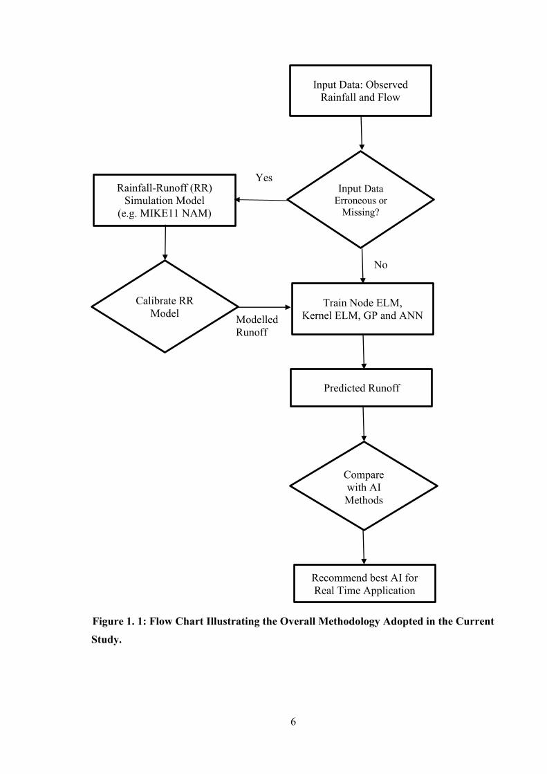
The overall flow chart illustrating the overall methodology adopted in the current study is

shown in Figure 1. 1.

6

Figure 1. 1: Flow Chart Illustrating the Overall Methodology Adopted in the Current Study.

Modelled Runoff

Input Data: Observed Rainfall and Flow

Input Data Erroneous or

Missing?

Rainfall-Runoff (RR) Simulation Model

(e.g. MIKE11 NAM)

Compare with AI Methods

Train Node ELM, Kernel ELM, GP and ANN

Predicted Runoff

Recommend best AI for Real Time Application

Calibrate RR Model

Yes

No

7

1.4. Scope of this Study

This study includes the following scope of works to understand the limitations (e.g.

prediction accuracies, run time etc) of some of the existing hydroinformatic approaches (e.g.

Artificial Intelligence techniques) and how these limitations can be improved using a

relatively new machine learning technique.

• Literature review.

• Genetic Programming (GP), Artificial Neural Network (ANN) and Extreme

Learning Machine (ELM) will be used for rainfall-runoff modelling/flood

forecasting.

• Historical rainfall and lagged observed flow will be used to train GP, ANN, and

ELM.

• Traditional rainfall-runoff model using MIKE11-NAM will be developed and

calibrated using observed flow.

• NAM output and historical rainfall be used as input to train GP for flood forecasting,

• The performance of GP will be improved using base flow parameter.

• Rainfall scenarios using long term historical rainfall time series (100 year) will be

generated by extending the drought season and fed into the GP.

• Future rainfall time series generated by varying the rainfall magnitude will be used

for flood forecasting for next 100 years.

• GP, ANN and ELM will be applied for the prediction real-time flows from three

catchments in Denmark, USA and Australia.

• Two types of ELM (node and Kernel based) techniques will be investigated for the

prediction of flood flows and compared with other techniques.

• The best method is recommended for the real-time application as a flood forecasting

tool.

8

1.5. Organisation of the Thesis

Chapter 2 describes the previous research works in the application of evolutionary

algorithm and data driven modelling techniques and the problems associated with their

application in rainfall-runoff modelling.

Chapter 3 describes the application of Genetic Programming (GP) and Artificial

Neural Network (ANN) in predicting flows using the rainfall and past historical observed

lagged flow. The long-term (>100years) prediction of flows is also described using hybrid

approach where GP is linked with MIKE11-NAM.

Chapter 4 demonstrates the use of a relatively new Artificial Intelligence (AI)

technique called, Extreme Learning Machine (ELM) for prediction hydrological flow series.

The performance of ELM (node based) is compared with other widely used data driven

modelling techniques including Standard Chaos Technique, Inverse Approach, ANN and

Evolutionary Computation (EC) based Support Vector Machine (SVM).

Chapter 5 presents the improvement of node based ELM’s performance by fine-

tuning the input parameters. The sensitivities of input parameters on the flow prediction,

higher lead days prediction and ELM’s extrapolation capability are also described in this

chapter. The performances of some of the best models are compared with GP and EC-SVM.

Chapter 6 applies the application of improved ELM called Kernel based ELM and

compares the performance and run time against node based ELM, GP and EC-SVM.

Chapter 7 describes the conclusion of this research works and recommends for

further studies.

9

CHAPTER 2

LITERATURE REVIEW

10

2. Literature Review

2.1. Introduction

The need for hydrological flow estimation and prediction is quite obvious to

complement field measurement especially when the catchment is very large and has scarcity

of hydrologic record. Gathering data by installing measurement equipment is sometimes

difficult in terms of cost and time as the flow estimation model requires long period of

hydrological information. This leads to the analysis of hydrologic response of the catchment

to future rainfall occurred on the catchment. Accordingly, research interests have been

concentrating on the development of efficient hydroinformatic approach to estimate the

flows yield from the catchment.

In this chapter, various techniques known in the rainfall-runoff model are first

reviewed especially the applications of conceptual models and data driven models. Review

on some recently emerging evolutionary techniques that were linked with data driven model

useful to solve complex problems and improve the prediction accuracy is also presented.

2.2. Conceptual Techniques in Rainfall-Runoff Model

In hydrological process, rainfall is converted to flows for the management of

catchment. The flow estimation process from the rainfall is reported to be highly non-linear

and is not easy to represent in the simple model (Singh, 1964; Kulandaiswamy and

Subramanian, 1967; Chiu and Huang, 1970). Usually, two approaches were applied, namely

conceptual approach and black box approach (Young and Wallis, 1985; Singh, 1988).

In the analysis of rainfall-runoff model, various conceptual methods were

developed with the advent of high performance computational techniques. Such methods

include MIKE11 NAM (Nielsen and Hansen, 1973), Sacramento Model (Burnash, 1995),

Tank Model (Sugawara, 1995), SWMM (Huber et al., 1988), XPRafts, RORB, URBS and

11

WBNM. In principal, conceptual methods generalise the hydrological cycle and predict the

flow from watershed. Some of these also take into account the soil moisture interconnection

with hydrologic cycle (Duan et al., 1992). However, depending on the level of details of

hydrological cycle included in the model, some parameters must be adjusted in order to

match model output to those observed from the catchment of interest. Fine tuning of these

parameters is usually performed manually. However, this manual approach is time

consuming to arrive at a satisfactory solution particularly when the calibration parameters

are large (Ibrahim and Liong, 1992). In these circumstances, automatic calibration

procedures were developed with computer technology. Development of automatic

calibrations (Madsen, 2000) schemes which is called optimization techniques, has been an

active research endeavours during the past decades.

Several optimization methods have been applied in the calibration process. These

traditional optimization techniques include linear, nonlinear, dynamic programming and

evolutionary algorithms. The detailed description of evolutionary algorithm is presented in

section 2.4.

2.2.1. Linear Programming

A linear programming gradient (LPG) method is presented by Alperovits and

Shamir (1977) in the optimal design of water distribution network by linearizing the

mathematical formulation (Atiquzzaman, 2004). Quindry et al. (1981), Fujiwara et al.

(1987), Kessler and Shamir (1989) and Eiger et al. (1994) also applied LPG successfully and

enhanced the functionalities (Morgan and Glulter, 1985; Fujiwara and Khang, 1990).

However, linearization of complex non-linear process in LP reduces its performance. It is

not always beneficial to linearise the problem as it may suffer losses and distort the original

problem (Atiquzzaman, 2004).

12

A linear programming model was introduced by Tu et al. (2003) for multipurpose

reservoir system operation. The reservoir operating rules was proposed to minimize the

drought impacts. The model efficiently allocated water to meet the planned demand during

normal periods of operation.

2.2.2. Non-Linear Programming

Chiplunkar et al. (1986) and Lansey and Mays (1989) applied non-linear

programming technique (NLP) (Su et al., 1987; Duan et al., 1990). Compared to LP, NLP

model can deal with more variables. However, Chiplunkar et al. (1986) often found that the

NLP model often converged prematurely to the local minima. In the last few decades, non-

linear programming algorithms that use gradient based algorithms, have been applied

widely. Gradient based technique can easily identify a relative optimum solution. However,

the method does not always provide optimal solution on a non-convex search space

(Atiquzzaman, 2004). Simpson et al. (1994) and Savic and Walters (1997) indicated that

NLP is also inadequate to deal with discontinuous search space and unable to provide

optimal solution (Gupta et al., 1999; Cunha and Sousa, 1999).

2.2.3. Dynamic Programming

Dynamic Programming (DP) has been adapted since 1960s in the water resources

engineering and management problem (Wong and Larson, 1968). In DP, the optimization

problem is sub-divided into stages where each stage is linked to the previous stage

(Atiquzzaman, 2004). The input of current state is transferred to the following stage. A two-

stage dynamic programming approach is proposed by Vamvakeridou-Lyroudia (1993). Lall

and Percell (1990) developed a dynamic programming based optimizer (GPO) and applied

in the gas transmission pipeline systems. They determined the optimized solution (feasible

13

strategy) by minimising the operation cost of the pipeline and satisfying several constraints.

DP produced satisfactory results to simple systems. However, the performance DP

deteriorated if the system was increased in size and the computational time increased

significantly (“the curse of dimensionality”) (Atiquzzaman, 2004).

During the past decade or so, population-evolution-based optimization schemes have

been extensively used for model calibration. The successful application of CRR model

depends heavily on how well the conceptual model is calibrated (Johnston and Pilgrim,

1976; Duan et al., 1992; Ibrahim and Liong, 1992; Liong et al., 1995a; Gan and Biftu, 1996;

Kuczera, 1997; Thyer et al., 1999). Gupta et al. (1999) mentioned that finding optimal

parameters for a CRR model may be difficult from the calibration process. Such problems

attributable to the data or information available for calibration cannot identify model

parameter values with acceptable precision and non-linear structural characteristics of CRR

models. Duan et al. (1992, 1293) identified five characteristics complicating the optimization

problem which are: (a) existence of several major regions of attraction into which a search

strategy may converge; (b) each major region of attraction may contain numerous local

optima; (c) the objective function surface in multi parameter space may not be smooth and

may not even be continuous; (d) the parameters may exhibit varying degrees of sensitivity

and a great deal of interaction. Duan et al. (1992), through their six-parameter conceptual

rainfall-runoff model called SIXPAR demonstrated in their study that the conceptual

rainfall-runoff model calibration problem is more difficult than had been previously thought.

They performed detailed analysis of the response surface of different objective functions on

the SIXPAR model and demonstrated the presence of multiple optima complicating the

conceptual rainfall-runoff model calibration. Finally, they stated that calibration of such

model requires sophisticated mathematical tools and some degree of expertise and

experience with the model.

14

2.3. Artificial Intelligence (AI) Technique

The AI approach is based on identifying a relationship between input and output

from the historical observed data without attempting to describe any of the internal

mechanisms. Professionals, researchers in water resources have been interested in data

driven modelling using AI approaches which are assumed to overcome some of the

drawbacks associated with conventional techniques (conceptual model). Such

techniques are proven to be an effective and efficient way to model the complex process

(e.g. RR) where the knowledge of the hydrological process is not required. Over the last

few decades, these tools have been useful operation tools in case of the absence of

hydrologic data such as evaporation data, catchment characteristics, etc. This has

attracted to the attention of researchers where accurate and timely estimation of flow

and flood forecasting is an extremely important issue in water industry as the existing

structural protection system is not adequate to reduce the flood risk. AI (also called

Black box model), according to Toth et al. (1999), is sometimes essential to predict the

flow in shortest possible time which will allow sufficient time for flood warning and

evacuation plan. Black box models for flood forecasting are most suitable tools,

especially when the catchment size is large. Application of AI technique has been very

popular as conceptual and physically based distributed models in the prediction of dam

inflows or natural catchment yield requires many parameters including catchment area,

slope, soil type, infiltration, drainage networks and their layout or their representations

in the model and meteorological data (rainfall and runoff data). The values of some of

these parameters, like infiltration rates, can only be determined through calibration.

Calibration of such models using a trial and error method, or optimization algorithm

needs knowledge and experience about the catchment, extensive effort specially for

15

larger catchment with lots of calibration parameters to be determined (Atiquzzaman and

Kandasamy, 2016a). Artificial intelligence (AI) based machine learning techniques have

proven superior in this modelling process (e.g flow prediction) compared to other

stochastic models including “Autoregressive (AR)”, “Autoregressive Moving Average

(ARMA)”, “Autoregressive Integrated Moving Average (ARIMA)” and

“Autoregressive moving average with Exogenous Inputs (ARMAX)” (Hsu et al., 1995

and Lohani et al., 2012). Over the last decades, AI techniques including Artificial Neural

Network (ANN) (Funahashi, 1989; Furundzic, 1998; Gallant and White, 1992; Anctil et

al., 2004; Jeevaragagam and Simonovic, 2012), Fuzzy Logic (FL) (Tayfur and Sing,

2006; Adeli and Sarma, 2006), Support Vector Machine (SVM) (Sivapragasam and

Liong, 2002, Yu and Liong, 2004), Chaos Theory (Yu et al., 2002), and Genetic

Programming (GP) (Lee and Suzuki, 1995; Rodriguez-Vazquez and Flemming, 1997;

Keijzer and Babovic, 1999; Jayawardena et al., 2005; Meshgi et al., 2015) have been

successfully utilized in many application around the world for their ability to recognize

non-linearity in complex hydrological process.

Generally, application of data driven models to predict hydrological flow series

(future discharges) requires an input of lagged discharges or meteorological data

(Akhtar et al., 2009). Prediction of hydrological flow at a location in a river was

performed by Karunanithi et al. (1994) using a cascade correlation algorithm. Flow data at

different locations along the river and along its tributaries was as input. The model performed

better than the commonly used conventional technique. Appropriate network structure,

presenting data to “Artificial Neural Network (ANN)” and training algorithms were also

presented. The study outcome revealed that lag time is more important in predicting stream

flows. Hsu et al. (1995) demonstrated that non-linear ANN models provided a more

representative rainfall-runoff relationship. They compared ANN results with ARMAX and

16

the conceptual Sacramento soil moisture accounting model. It was reported that the models

tend to fit the higher flows quite well. However, the low flow prediction is not so good for a

one-step ahead prediction. Fernando and Jayawardena (1998) also modelled this by using

Radial Basis Function neural network (RBF-NN). They showed it performed better than the

ARMAX. ANN with multi-layer perceptron (MLP) networks trained with gradient-based

methods has been used in many applications. Traditionally, the weight vectors in ANN

models is determined using back-propagation (BP) algorithm by minimizing the mean

square error between the measured and forecasted discharges of the hydrological process.

However, the performance of ANN depends on network architecture (e.g. number of hidden

layers, the number of neurons, activation functions etc), performance criteria, division and

pre-processing of data, and determining appropriate model inputs (Maier and Dandy, 2000).

Cigizoglu (2003) studied the application of ANN for forecasting of daily flows for a river in

Turkey. Their analysis demonstrated ANN’s superior capability compared to conventional

models (e.g. AR and regression models). Application of data-driven modelling methods has

been made to quantify the uncertainty associated with the prediction. Kingston et al. (2005)

highlighted ANN’s failure to account for prediction uncertainty as the quantification of

uncertainty associated with ANN’s parameter, namely, weights is complex and difficult.

They proposed Bayesian training method to assess ANN’s weight uncertainty. Peters et al.

(2006) used HEC-RAS model to train the multilayer feed forward ANN and to replace one-

dimensional hydrodynamic modelling system with ANN. They showed that ANN model

performed well in terms of decrease in computational time especially for online flood

forecasting. Wang et al. (2005) improved the performance of ANN with self-organising

polynomial neural network (SOPNN). They demonstrated the capability of SOPNN in

selection of appropriate model inputs, optimization of the network structure and error

minimisation. SOPNN was applied to runoff prediction and it was found that SOPNN

17

performed better than the group method of data handling (GMDH) and the traditional back-

propagation network (BPN). Mittal et al. (2012) proposed a dual (combined and paralleled)

artificial neural network (D-ANN) to estimate the extreme runoff values. They compared the

performance of D-ANN with common feed forward ANN (FF-ANN). D-ANN performed

better than FF-ANN. The relationship between input and output vectors were established

using three steps: (1) compilation of the statistics of rainfall and the corresponding runoff

𝑄𝑡 = 𝑓(𝑅𝑡−9, 𝑅𝑡−8, 𝑅𝑡−7, 𝑄𝑡−1, 𝑄𝑡−2), where R and Q represent the rainfall and runoff

values at time “t”; (2) estimation of predicted values and errors of the runoff values (𝜀 =

𝑦 − ), where 𝑦 is observed value of runoff, predicted value of runoff and 𝜀 value of error;

(3) estimation of error corresponding to the predicted runoff 𝜀𝑡 =

𝑓(𝑅𝑡−9, R𝑡−8, 𝑅𝑡−7, 𝑄𝑡−1, 𝑄𝑡−2). The ultimate predicted value of runoff was derived by

summing the predicted value and the error. The model was applied on a real case study on

Kolar River basin in India. In the application, it was demonstrated that though both D-ANN

and FF-ANN produced similar behaviour but D-ANN was able to predict the peak value

better than FF-ANN. According to Chen and Chang (2009), a very simple ANN network

architecture may not accurately predict while too complex architecture may reduce its

generalization ability due to over-fitting. Uncertainty in streamflow prediction was assessed

by Boucher et al. (2009) based on ensemble forecasts using stacked neural network. Instead

of forecasting a single value (e.g. one-day-lead prediction), they predicted an ensemble of

stream flows which was then used to fit a probability density function to assess the

confidence interval as well as other measures of forecasts uncertainty. The uncertainty

associated with prediction of water levels (or discharges) was analyzed by Alvisi and

Franchini (2011). They introduced fuzzy numbers to determine the weights and biases of

neural network to estimate prediction uncertainty of water levels and discharges. The

comparison of this fuzzy neural network method with Bayesian neural network and the local

18

uncertainty estimation model demonstrated the effectiveness of the proposed method where

the uncertainty bands had slightly smaller widths than other data-driven models. Alvisi and

Franchini (2012) found better accuracy in forecasting water levels and narrower uncertainty

band width compared to Bayesian neural network using Grey neural network (GNN). Here

the parameters are represented by unknown grey numbers that lie within known upper and

lower limits. The grey parameters are searched in way that the grey forecasted river stages

include at least a preselected percentage of observed river stages. Sing et al. (2015) applied

ANN to establish relationships between rainfall and temperature data with runoff from an

agricultural catchment (973 ha) in Kapgari (India). Several resampling of short length

training datasets using bootstrap resampling based ANN (BANN), found solutions without

over-fitting. A ten-fold cross-validation (CV) technique based ANN was also applied to

obtain unbiased reliable testing results. Sing et al. (2015) demonstrated that BANN provides

more stable solutions and was able to solve problems of over-fitting and under-fitting than

ten-fold CV based ANN. Gholami et al. (2015) achieved high degree of accuracy in the

prediction groundwater fluctuation using dendrochronology (tree-ring diameter) and ANN

(multilayer perceptron, MLP). Rasouli et al. (2012) applied three machine learning methods

including Bayesian Neural Network (BNN) for streamflow forecasting using different

combination of local meteo-hydrologic observations and climate indices. They found that

BNN outperformed the other nonlinear models. Chen and Chang (2009) proposed an

evolutionary algorithm (Genetic Algorithm (GA)) based ANN (EANN) to define the optimal

network architecture and for prediction of real-time inflows to the Shihmen Reservoir in

Taiwan. They demonstrated that EANN performed better than the ARMAX stochastic

model. Chen and Chang (2009) also stated that the performance of ANN depends on network

architecture (e.g. inputs, number of hidden layers, the number of neurons and activation

functions) and noted that very simple network architecture of ANN may not accurately

19

predict while too complex architecture may reduce its generalization ability due to over-

fitting. Wu and Chau (2011) found that the performance of ANN can be improved

significantly if the input data is preprocessed with Singular Spectrum Analysis (SSA).

The performance of ANN was improved by combining with other techniques (e.g.

hybrid methods) (Chen et al., 2915). For example, Deka and Chandramouli (2009) proposed

Fuzzy Neural Network (FNN) hybrid model to study the operation of a proposed

multipurpose reservoir system and found that FNN is highly adaptive, flexible, easy to build.

Adaptive Neural-based Fuzzy Inference System (ANFIS) significantly improved on ANN

predictions for reservoir prediction (Bhakra Dam, India, Lohani et al., 2012); for forecast of

daily flood discharge (Yom River Basin, Thailand, Tingsanchali and Quang, 2004; and Ajay

River Basin in Jharkhand, India, Mukerji et al. 2009), and for event-based rainfall-runoff

modeling using lag time (Talei and Chua, 2012).

Fuzzy rule based models are based upon the fuzzy set theory. Fuzzy set theory

differs from the classical theory of crisp sets. A fuzzy set is a class of objects which is

characterised by a membership function. The membership functions for each object assign a

grade ranging between zero and one (Zadeh, 1965). Fuzzy set comprises of ordered pairs of

values, (𝑥, 𝜇𝑎(𝑥)), where x is an element of numerical basic set A and where 𝜇𝑎(𝑥) is the

degree of membership of x. If the grade for membership function is 1, this means that x

entirely belongs to the fuzzy set. Zero grade, on other hand indicates that x does not belong

to the fuzzy set at all. Values in between mean that x belongs to the set to some degree.

Tayfur and Singh (2006) described a general fuzzy system consists of four steps –

fuzzification, fuzzy rule base, fuzzy output engine, and defuzzification. In fuzzy logic

application, firstly the input data are converted to degree of membership functions. Secondly,

fuzzy rule base defines a list of rules that include all possible relations between inputs and

outputs. These rules are generally expressed in the IF-THEN format. There are two types of

20

expression of rules used in fuzzy application which are called ‘Mamdani’ and ‘Sugeno’. In

Mamdani rule system, the consequent of the input variable is expressed as verbally.

However, in Sugeno rule system, the consequent part of the fuzzy rule is expressed as a

mathematical function of the input variable. Thirdly, the fuzzy inference system engine take

into account of all the fuzzy rules in the fuzzy rule base and transform them to a set of output.

Finally, defuzzification converts the resulting fuzzy outputs from the fuzzy inference engine

to a number. There are several defuzzification methods available which are centre of gravity

(COG), bisector of area (BOA), mean of maxima (MOM), left-most maximum (LM), and

right most maxima (RM) etc. Fuzzy logic has been widely applied in hydrological modelling

for the last two decades. Fuzzy conceptual rainfall-runoff framework was proposed by

Ozelkan and Duckstein (2001) where every element of the rainfall-runoff model was

assumed to be uncertain. Fuzzy rules, applied to different operational modes and the

parameter identification process was examined using fuzzy regression techniques. The

methodology was applied to different types of conceptual models including linear,

experimental two parameters and Sacramento Soil Moisture Accounting Model that enabled

the decision maker to understand the model sensitivity and the uncertainty stemming from

the elements of the model. Tayfur and Sing (2006) applied ANN and fuzzy logic (FL) for

predicting event based rainfall-runoff and the results were compared against the “kinematic

wave approximation (KWA)”. A three layered “feed-forward ANN” was developed using

the “sigmoid function” and the “backpropagation algorithm”. The triangular fuzzy

membership functions were applied to develop the fuzzy logic model for the input and output

variables. They described that ANN and FL require long historical data compared to KWA.

But KWA model involves many parameters for which field estimation is needed. Adaptive

Neuro-Fuzzy Inference System (ANFIS) and ANN were applied by Tingsanchali and Quang

(2004) to forecast the daily flood flow of the Yom River Basin in Thailand. They

21

demonstrated that ANFIS performed better than ANN multilayer perceptron model. Though

different types of ANN together with Fuzzy Logic have been successfully applied to solve

complex hydrological processes, it suffers from some major limitations (ASCE Task

Committee, 2000 a and b), for example,

• choosing optimal network architecture is an issue;

• does not provide a direct relationship between the input and output variables; and

• does not help in advancing the scientific understanding of hydrological process.

Cui et al. (2014) examined the impact of topographic uncertainty in their rainfall-

runoff model (TOPMODEL). The performance of TOPMODEL is influenced by the grid

size of the digital elevation model (DEM) that defines the topography. The relationship

between DEM resolution and TOPMODEL performance was investigated using fuzzy

analysis technique. Different grid sizes of the DEM ranging from 30m to 200m were used

in TOPMODEL. It revealed that the best results were produced with fuzzy technique for the

30m resolution. Cheng et al. (2002) adopted a parallel Genetic Algorithms (GA) with Fuzzy

Optimal model in a cluster of computers to reduce the computational run time required to

optimize the rainfall-runoff model (Xinanjiang) and to improve the quality of the results. As

the problem was partitioned into smaller pieces, their proposed hybrid approach achieved

the superior results quicker than GAs.

Over the last several decades, parallel to ANN and Fuzzy Logic, Genetic

Programming (GP) has been applied to solve various hydrological/hydraulic problems,

such as rainfall-runoff relationship from synthetic data, sediment transport modelling,

prediction of bridge pier scouring (Azamathulla et al., 2010), salt intrus ion in estuaries

and flow over a flexible vegetated bed (Babovic, 1996; Babovic and Abbott, 1997).

Babovic and Abbott (1997) mentioned that GP can be used to model single non-linear

22

reservoir behaviour of a hypothetical catchment simulated by RORB. Whigham and

Crapper (2001) applied Genetic Programming to predict the runoff from 2 catchments

using only previous rainfall data. One of the catchments is a moderately fast response

catchment and the other, a rapid response catchment. They found that Genetic

Programming was able to distinguish the slow response from the rapid response of the

catchment and reacted accordingly by incorporating the average rainfall terms in the

resultant expression. Makkeasorn et al. (2008) showed GP performed better than neural

networks (NN) for forecasting discharges in a semi-arid watershed in South Texas, USA

by including sea surface temperature, spatio-temporal rainfall distribution,

meteorological data and historical streamflow data. The application of GP in real-time

runoff forecasting was also demonstrated by Liong et al. (2002). Liong et al. (2002)

applied GP as a forecasting tool in a catchment with a drainage area of 6 km 2. Different

storm intensities and durations were considered to train and verify GP results. The

functional relationship between rainfall and runoff derived from GP showed that the

prediction accuracy of GP in terms of RMSE is reasonably good. Savic et al. (1999)

found in their study that GP performed better compared to conceptual hydrological

model (e.g. HYRROM). Application of GP demonstrated by Khu et al. (2001) in real-

time runoff forecasting showed that GP played as an error updating scheme to

complement traditional hydrological model (MIKE11/NAM). GP was able to predict

the runoff for all updating intervals not exceeding the time of concentration of the

catchment. They also found that non-dimensionalising the variables enhanced the

prediction accuracy. Ten storm events were considered to infer the performance of GP

in updating NAM output. The best functional form with minimum RMSE is as follows:

𝑸𝑰𝑴𝑷𝒕+𝟏 = 𝑸𝑺𝑰𝑴𝒕 + 𝟎. 𝟎𝟎𝟗 + 𝟏. 𝟔𝟏𝜺𝒕 − 𝟎. 𝟔𝟒𝟒𝜺𝒕−𝟏 + 𝟎. 𝟎𝟖𝟕𝜺𝒕(𝑸𝑺𝑰𝑴𝒕−𝟐 − 𝑸𝑺𝑰𝑴𝒕−𝟏

23

Where, 𝑸𝑰𝑴𝑷𝒕+𝟏 is improved discharge at time 𝒕 + 𝟏; 𝑸𝑺𝑰𝑴𝒕 is simulated discharge at

time 𝒕; 𝜺𝒕 is prediction error at time 𝒕. GP also produced comparable results with two

other updating methods such as the auto-regression and Kalman Filter. In applied

engineering, GP is frequently used to recognise the relationship between the complex

hydrological parameters. Rodriguez-Vazquez et al. (2012) proposed GP and Genetic

Algorithm (GA) for rainfall-runoff modelling of a sub-basin located near Mexico City.

They developed two different models for the analysis. The first was a multi-objective

optimization based GP model for determining the structures and parameters of non-

linear auto-regressive models (NARMAX). The second was a GA based model that

optimized the parameters of a non-conventional rainfall-runoff model. Their analysis

concluded that the multi-objective optimization based GP model best fitted the analysed

storms of interest. Recently, Nourani et al. (2013) included watershed geomorphological

features as spatial data together with temporal data in GP for rainfall-runoff modelling.

Two separate scenarios, namely separated gemorphological GP (SGGP) and integrated

gemorphological GP (IGGP) models and their application were described. The

geomorphological parameters or the spatial data includes area, slope and curve number

for sub-basin were considered in addition rainfall and runoff time series. Separate GP

models were developed for each sub-catchment in SGGP where as all the sub-catchment

spatial and temporal parameters were integrated in IGGP. From the application of these

techniques to Eel River Watershed, they found these models could compensate the lack

of temporal data. Specifically, SGGP model for the sub-basins could distinguish the

dominant variables of the sub-basins in the process and IGGP can be a reliable tool for

spatial and temporal interpolation of runoff through the watershed. IGGP was able to

fill up the data gaps in other stations.

24

SVM is another powerful AI technique that has been successfully applied in flow

forecasting, rainfall-runoff modeling (Sivapragasam et al. 2001) and streamflow forecasting

(Chiogna et al., 2018). SVM is a statistical method that resolves the problem similar to a NN

but the nature of its underlying functional form is not assumed a priori. In other words, SVM

can be seen as an approximate implementation of the method of structural risk minimisation.

In this process, learning from data is actually to choose from the given set of functions which

best approximate the measured output. The best approximation represents the smallest value

of the risk. However, if the training examples are limited, this approach does not guarantee

a small actual risk. To overcome this limitation, statistical learning theory has been

introduced. In this method, the structural risk is minimised by controlling the estimate of risk

and the confidence interval of this estimate (Vapnik, 1999). Chiogna et al. (2018) proposed

SVM with hydrological model (Soil Water Assessment Tool) output, the hydropower energy

price and the day of the week to capture sudden fluctuations in river stage caused by the

hydropower production company in Upper Adige River basin in North-East Italy. They

found that that SVM was able to reproduce the hydropeaking and performed better than

SWAT under low flow condition when the streamflow was impacted by the hydropower.

SVM was applied by Sivapragasam (2002) and Liong and Sivapragasam (2002) to predict

the stage in the city of Dhaka, Bangladesh using daily water level data measured at five

gauging stations (Liong et al., 1999). The results showed that SVM performed better than

ANN (Liong et al., 1999) in terms of RSME and R2. Similarly, SVM was shown to be

comparable or better than ANFIS and GP, for application in forecast of monthly river flow

(Wang et al. 2009) and short term river flow (Heihe River, Northern China, He et al. 2014).

Sivapragasam (2002) applied SVM to rainfall-runoff modelling using six storm events that

occurred in Upper Bukit Timah catchment, Singapore. The results showed the robustness of

SVM compared to multi-layered feed-forward ANN.

25

SVM was further improved by reducing the noise from input data using Singular

Spectrum Analysis (Sivapragasam et al., 2001), optimization of SVM parameters using

Evolutionary Computation based Algorithm (EC-SVM) (Yu et al., 2004) and Particle Swarm

Optimization algorithm (Wang et al. 2013). Lin et al. (2006) reported SVM as a powerful

tool that could overcome some of the drawbacks that were evident in ANN: (1) finding

global solutions, (2) over-fitting unlikely, (3) generating non-linear solutions using the

Kernel Function, and (4) obtaining optimized solutions using a limited training dataset.

While SVM overcame some drawbacks of ANN (finding global optimized solutions and

over-fitting, Lin et al. 2006), it required a long simulation time for large complex problem,

and in the selection of an appropriate kernel function and associated parameters (C and ε).

Fotovatikhah et al. (2018) reviewed the available AI and computational intelligence (CI)

methods in the literature including ANN, fuzzy sets, wavelet models, SVM, EC and hybrid

methods employed in hydrology, flood and waste flow prediction. They found that EC and

SVMs showed lower error rates compared to other machine learning and soft computing

techniques. Yu et al. (2004) presented a combined application of Chaos Theory and SVM

where the parameters were optimized with an EA to reduce prediction error. In SVM,

Gaussian Kernel function, being more suitable, was applied to hydrological time-series

application (Liong and Sivapragasm, 2002). An EA engine, called Shuffled Complex

Evolution (SCE), was applied to determine five parameters, i.e. time delay, embedding

dimension and three SVM parameters (tradeoff between empirical error and model

complexity, insensitive loss function, and width of Gaussian kernel function). EA based

SVM (EC-SVM) was used to predict runoff time-series for catchments including the

Tryggevælde Catchment, Denmark and the Mississippi River, USA. The results showed that

EC-SVM improved the prediction accuracy compared to standard chaos technique, Naïve,

ARIMA and Inverse Approach. Wang et al. (2013) applied an EA, called particle swarm

26

optimization (PSO), to determine SVM parameters. They further proposed ensemble

empirical mode decomposition (EEMD) for decomposing annual rainfall series in SVM to

avoid model over-fitting or under-fitting. The proposed model (PSO-SVM-EEMD)

improved the rainfall-runoff forecasting significantly compared to ordinary least-square

regression model and ANN. Sivapragasam et al. (2001) enhanced the performance of SVM

by pre-processing the input data using a noise-reduction algorithm, Singular Spectrum

Analysis (SSA). SSA was coupled with SVM and used to predict the flows from the

Tryggevælde Catchment (Denmark). It improved the prediction accuracy compared to the

non-linear prediction (NLP) method.

Literature on the application of AI approaches including ANN, ANFIS, SVM and

GP in hydrological time-series prediction indicates that their performances are not consistent

for all applications and it is difficult to state which method is superior. Superior performance

depends on appropriate parameters and network configurations. Researchers have attempted

to improve the performance of these methods using hybrid approach (ANFIS) or by

combining them with other algorithms (EC-SVM) to optimize the parameters. However,

they still require numerous iterations and significant computational time to generate

optimum solutions. To overcome this, Huang et al. (2006) proposed a learning algorithm,

called “Extreme Learning Machine (ELM)”. ELM determines weights related output

analytically with randomly generated input weights. The performance of ELM has been

compared by Huang et al. (2006) with conventional neural network (BP) and SVM on some

benchmarking problems in the function approximation and classification areas. Huang et al.

(2006) reported that ELM is capable of approximating any continuous function and

implementing any classification. ELM learns faster (Taormina and Chau, 2015) and is stable

with a wide range of number of hidden nodes. ELM was also applied by Taormina and Chau

(2015) in the selection of input variables for rainfall-runoff modelling. They obtained most

27

accurate solutions with ELM is coupled with Binary-coded discrete Fully Informed Particle

Swarm Optimization (BFIPS). The performance of ELM depends on the activation function

and the random assignment mechanism. With appropriately selected activation function and

random mechanism, ELM does not degrade the generalization capability (Lin et al., 2014).

Numerous experiments and applications have demonstrated the effectiveness and efficiency

of ELM (Huang et al., 2006). Atiquzzaman and Kandasamy (2016b) demonstrated that

ELM’s learning speed and accuracy were comparable to Standard Chaos Technique, Inverse

Approach and EC-SVM in the forecasting of hydrological time-series (refer to Chapter 4).

However, the robustness of ELM’s performance (improved accuracy) on different input

parameters, longer lead day prediction and extrapolation capability was not investigated by

Atiquzzaman and Kandasamy (2016b) (refer to Chapter 5).

The following sections present the brief description of Artificial Neural Networks

(ANN), Genetic Programming and Extreme Learning Machines as this study applies these

three AI techniques. ANN and GP are applied in this study for comparison against ELM.

2.3.1. Brief Description of Artificial Neural Network

A lot of works has been particularly carried out in the application of ANN in stream

flow forecasting and runoff modelling due to its capability to reproduce the unknown

relationship existing between a set of input and output variables. American Society of Civil

Engineers (ASCE) has officially formed a committee on application of ANN in and they

reported that since the early nineties, ANNs have been successfully used in R-R modelling

and other hydrology related areas such as stream-flow forecasting, ground-water modelling,

water quality, water management policy, precipitation forecasting, hydrologic time series,

and reservoir operations.

28

Artificial Neural Network (ANN) is a network that connects many simple elements

called neurons. Each neuron has a small amount of local memory. The neuron connections

are established through communication channels which carry numeric data encoded by

various means. Neurons become active when it receives data through the communication

channels.

The architecture of ANN follows the model similar to human brain and nerve cells.

Historically, much of the motivation to build ANN came from the desire to produce artificial

systems capable of mimicking the behaviour of human brain. Neural Network model derives

the statistical structures present in the input data set by using the architecture and learning

paradigms. The information acquired after learning the data structure is stored at the

connections between the elements of the neural architecture. At the beginning, the

architecture is not structured and the learning algorithms extracts the regularities present in

the data by finding a suitable set of synapses during the process of observation of the

examples. Thus, ANNs solve problems by self-learning and self-organization i.e. the

network recognizes the features of input data itself and displays its findings. They derive

their intelligence from the collective behaviour of simple computational mechanisms at

individual neurons.

In ANN, there are two types of architectures including feed-forward and recurrent

architectures. The feed-forward architecture allows connections only in one direction and

the neurons are arranged in layers, starting from a first input layer and ending at the final

output layer with one or more hidden layers. The information passes from the input to the

output side. The recurrent architecture, however, permits back-coupling and any type of

connections is allowed. This is generally achieved by recycling previous network outputs as

current inputs, thus allowing for feedback.

29

Feed-forward network is usually used in hydrological problem as the recurrent

architecture based models are significantly more complex in terms of time and storage

requirements. This study considers only ANN with a feed-forward architecture. A 3-layered

feed-forward architecture is shown in Figure 2. 1. The 3 layers are called input, hidden output

layers. Each layer consists of several neurons which are interconnected by weight functions.

The input variables (observed data) are fed to input neurons directly. The variable

information is passed on to hidden and output layers through the interconnections between

the neurons. The neurons in input layer transform via weight functions which are estimated

through this process. The transformation is performed in two stages as shown below

(Sivapragasam and Muttil, 2005):

Determining Weighted Sum.

“Input from each neuron is multiplied with weights and a weighted sum is

performed”:

(1)

where “Yj(s) = weighted sum for neuron j in layer s; wij(s-1) = weight in the link

between neuron j in layer s and neuron i in layer (s-1); and xi(s-1) = input from neuron

i in layer s-1”.

Selecting Activation Function.

An activation function, F(s), such as the sigmoid function expressed as:

( ) )(1

1sYj je

sF−

+=

(2)

Fj(s) is the output of the neuron j in layer s.

Y s w s x sj ij ii

n

( ) ( ). ( )= − −=

1 10

30

Figure 2. 1: 3-Layered Feed Forward Neural Network Architecture

Initially, ANN generates the weights related to the interconnections randomly. In

this process, a learning rate (α) and a momentum rate (β) are defined. The learning rate plays

an important role and controls the variation (incremental change) of interconnecting weights.

During the iterative training process, the variation in the weight functions is controlled by

the learning rate based on the percentage of the difference between the observed and model

output. If the high learning rate is selected, larger weight change is observed, and the model

learns the input dataset quickly. The momentum rate ensures the model from being trapped

to local optima and increase the rate of learning at the same time. The change in the previous

interconnection weights is multiplied by the momentum rate. The relationship between the

learning rate and momentum rate is described as:

(3)

where ∆wij(s) = “weight adjustment between node j in layer s and node i in layer (s-1)”;

𝛿j(s) = “local or instantaneous gradient”; and

xi(s) = “input of neuron j from previous layer’s neuron i".

w s s x s w sij j i ij( ) ( ) ( ) ( )= + − 1

31

Equation 3 demonstrates that the momentum rate (β) increases the rate of variation

of weight when the local gradient component is in the same direction as that of the learning

component. Alternatively, the learning rate becomes faster when the error backpropagation

is downward and vice versa.

ANN model is trained with a list of input data. The model adjusts the

interconnection weights and computes the desired output until some termination criteria are

met. The trained ANN model with the optimized interconnection weights, can be readily

used to produce outputs for a set of known inputs.

2.3.2. Brief Description of Genetic Programming

“GP is a domain-independent automatic programming for evolving computer

programs to solve, or approximately solve problems” (Koza, 1992, 1997; Liong et al., 2002).

GP which is a member of EA family, is actually a generalization of genetic algorithm (Aytek

and Kisi, 2008). Poli et al. (2008) defined “Genetic programming (GP) is an evolutionary

computation technique that automatically solves problems without requiring the user to

know or specify the form or structure of the solution in advance”.

GP provides a transparent and structured system compared to other AI approach

such as ANN, as ANN produces their knowledge in terms weight matrix that is sometime

not accessible to human understanding (Savic et al., 1999). Scientists, researchers and water

manager usually focus on the agreement of predicted and observed behaviour of a complex

hydrological process using some kind of fixed relationship. If the comparison is accepted,

the model is considered to be correct within that context (Babovic and Keijzer, 2002). Hence,

GP can mimic this complex relationship and derive the governing equations directly from

measurement. Genetic Programming has the advantage of providing inherent functional

32

relationship explicitly over ANN. So, GP induced rainfall-runoff relationships can be an

alternative to commonly used rainfall-runoff models.

GP uses optimization mechanism to evolve simple program where Darwin’s natural

selection theory of evolution is applied to progressively generate the offspring from better

parents. In GP, trial parent programs are repeatedly modified in the search for better or fitter

solutions (Langdon, 1998). In this process, the quality criteria are defined to improve the

accuracy of EAs. These criteria are then used to measure and compares solution candidates

in a stepwise refinement of a set of data structures and return an optimal or near optimal

solution after a number of generations (Jayawardena et al., 2005). The accuracy of solution

depends on the level of noise in the data set. If the data is noise free, GP generates a function

in symbolic form which is defined by Liong et al. (2002) as symbolic regression. The

symbolic regression is error driven evolution and may be linear, quadratic or higher order

polynomial. GP has been extremely popular due to the success at searching complex non-

linear spaces and the robustness in practical application.

2.3.2.1. Generation of Offspring from Parent Population

Population in GP consists of functional relationship or computer program. In order

to create new relationship from parent relationship, the parent relationships are represented

by parse tree structures composed of function set and terminal set (see Figure 2. 2). The

functions are mathematical or logical operators and terminals are constants and variables.

These trees are dynamically modified by genetic operators which are called selection,

crossover and mutation to optimize its fitness value in the evolution process. The genetic

operator is applied to select individuals. Selection process involves some probabilistic

approach to copy individuals from previous generation to the next generation based on

fitness value. After selection, crossover and mutation are applied. Crossover operator inter-

33

changes randomly selected subtrees of each chosen parent pair to generate syntactically

correct offspring. Figure 2. 3 shows the crossover of two parent population. After the

crossover, the program probabilistically selects a single parental solution program from the

population based on objective function value and performs mutation operation. There are

several types of mutations possible in the process. For example, two of them are: (1) the

child population can be mutated by replacing a function or a terminal with another function

or a terminal; and (2) the whole subtree of a child population can be interchanged by another

subtree. The subtree in the process can be generated using the same approach applied at the

beginning to generate the initial population of points. The final solution is shown in Figure

2. 4.

Figure 2. 2: Parent Population in GP (Source: Liong et al., 2002)

34

Figure 2. 3: Child Population in GP (Source: Liong et al., 2002)

Figure 2. 4: GP Parse Tree Representing sqrt(b2-4ac)-b/2a (Source: Liong et al., 2002)

2.3.2.2. Working Mechanism

The basic steps of GP (Figure 2. 5) are described as follows:

1. Create a set of initial population of points/solutions.

2. Evaluate each solution (parse tree) and assign the fitness.

35

3. Generate a subset of population of points according to their objective function values

(fitness). Solutions with higher fitness values will be selected to produce offspring

(children).

Figure 2. 5: Flow Chart of Genetic Programming (Source: Liong et al., 2002)

4. Selects pairs of solutions randomly from the subset of population of points for mating

and apply crossover operation. Crossover will interchange the genetic components

between two selected points;

5. Choose a crossover location where the genetic materials of the parent population will

be interchanged (binary bit) to produce child population.

36

6. Apply mutation operation which randomly select a genetic information (0 or 1) of

the solution and change it from 0 to 1 or vice versa.

7. Copy the resulting mutated child chromosomes into the new population.

8. Evaluate the fitness value (performance) of the new population.

9. Repeat steps 3-8 until some termination criteria are met.

2.3.3. Brief Description of Extreme Learning Machine (ELM)

Extreme Learning Machine (ELM) is a relatively new AI techniques developed by

Huang et al. (2006). ELM is a single-hidden layer feed-forward neural network (SLFN) that

provides efficient unified solutions where the input weights and hidden layer biases are

chosen randomly (Huang et al., 2006). ELM’s hidden node parameters are independent

between the hidden layer and the training data which means that it generates the hidden node

parameters without depending on training data. However, ELM’s connections with output

neurons are adjustable. ELM determines weights related to output analytically with

randomly generated input weights. ELM transforms the training of Feed-Forward Neural

Network into a linear problem in which only connections with output neurons are adjusted.

Thus, the well-known generalized inverse technique is directly applied for the solutions.

ELM’s learning algorithm is much simpler, and the learning speed is extremely

fast as it avoids iterative tuning to determine the weights. The advantages of ELM are: (1)

faster learning speed than conventional method; (2) learns with single iteration; (3) better

generalization performance; (3) automatically determines all the network parameters

analytically; (4) suitable for many nonlinear activation function and kernel functions; (5)

straightforward in reaching solutions without facing issues like local minimum, improper

learning rate and overfitting; (6) suitable for online and real-time applications; and (7) a

viable alternative technique for large-scale computing and machine learning.

37

The mathematical equation for ELM can be formularized as (Figure 2. 6):

𝑓𝐿(𝑥) = ∑ 𝛽𝑖𝐺(𝑎𝑖, 𝑏𝑖, 𝑥𝑗) =𝐿𝑖=1 ∑ 𝛽𝑖𝑔(𝑎𝑖. 𝑥𝑗 + 𝑏𝑖

𝐿𝑖=1 ) (4)

where, 𝑎𝑖 is the weight vector connecting the ith hidden node and the input variables

and 𝑏𝑖is the bias of the ith hidden node, L is random hidden nodes; βi is the weight connecting

the hidden node and the output node and 𝑔(𝑥) is activation function (example, sigmoidal

function: 𝑔(𝑥) = 1/(1 + exp (−𝑥)); 𝑥 ∈ 𝑅𝑛 and 𝑎𝑖 ∈ 𝑅𝑛 ).

Figure 2. 6: Structure of Neural Network

When the difference between the target (𝑡𝑗) and the model 𝑓𝐿(𝑥) = 𝑦𝑗 is zero for

a time series of N samples,

∑ ||𝑦𝑗 − 𝑡𝑗||𝐿𝑗=1 = 0 (5)

where, J = 1, …N.

This means:

∑ 𝛽𝑖𝑔(𝑎𝑖. 𝑥𝑗 + 𝑏𝑖𝐿𝑖=1 ) = 𝑡𝑗 (6)

Equation (6) can be written as:

𝐻𝛽 = 𝑇 (7)

where H is called hidden layer output matrix of SLFN.

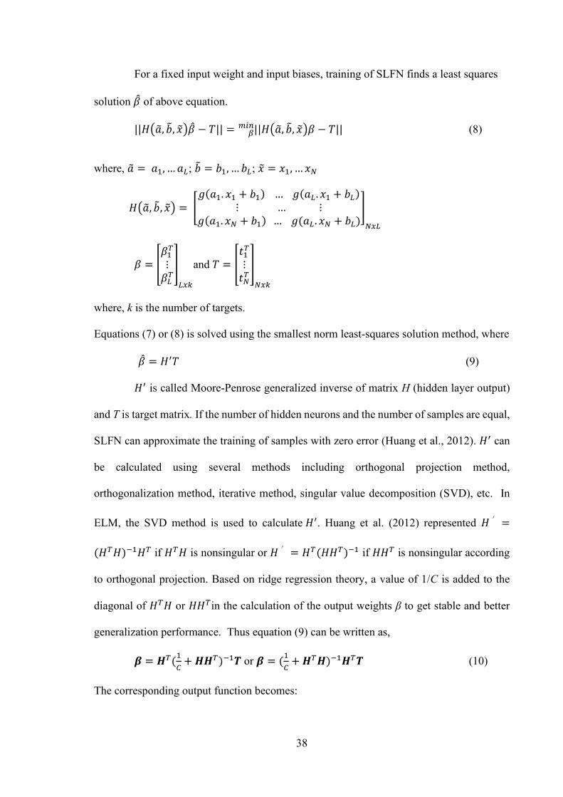
38

For a fixed input weight and input biases, training of SLFN finds a least squares

solution of above equation.

||𝐻(, , ) − 𝑇|| = ||𝐻(, , )𝛽 − 𝑇||𝛽𝑚𝑖𝑛 (8)

where, = 𝑎1, … 𝑎𝐿; = 𝑏1, … 𝑏𝐿; = 𝑥1, … 𝑥𝑁

𝐻(, , ) = [𝑔(𝑎1. 𝑥1 + 𝑏1) … 𝑔(𝑎𝐿 . 𝑥1 + 𝑏𝐿)

⋮ … ⋮𝑔(𝑎1. 𝑥𝑁 + 𝑏1) … 𝑔(𝑎𝐿 . 𝑥𝑁 + 𝑏𝐿)

]

𝑁𝑥𝐿

𝛽 = [𝛽1

𝑇

⋮𝛽𝐿

𝑇]

𝐿𝑥𝑘

and 𝑇 = [𝑡1

𝑇

⋮𝑡𝑁

𝑇]

𝑁𝑥𝑘

where, k is the number of targets.

Equations (7) or (8) is solved using the smallest norm least-squares solution method, where

= 𝐻′𝑇 (9)

𝐻′ is called Moore-Penrose generalized inverse of matrix H (hidden layer output)

and T is target matrix. If the number of hidden neurons and the number of samples are equal,

SLFN can approximate the training of samples with zero error (Huang et al., 2012). 𝐻′ can

be calculated using several methods including orthogonal projection method,

orthogonalization method, iterative method, singular value decomposition (SVD), etc. In

ELM, the SVD method is used to calculate 𝐻′. Huang et al. (2012) represented 𝐻′ =

(𝐻𝑇𝐻)−1𝐻𝑇 if 𝐻𝑇𝐻 is nonsingular or 𝐻′ = 𝐻𝑇(𝐻𝐻𝑇)−1 if 𝐻𝐻𝑇 is nonsingular according

to orthogonal projection. Based on ridge regression theory, a value of 1/C is added to the

diagonal of 𝐻𝑇𝐻 or 𝐻𝐻𝑇in the calculation of the output weights β to get stable and better

generalization performance. Thus equation (9) can be written as,

𝜷 = 𝑯𝑇(1

𝐶+ 𝑯𝑯𝑇)−1𝑻 or 𝜷 = (

1

𝐶+ 𝑯𝑇𝑯)−1𝑯𝑇𝑻 (10)

The corresponding output function becomes:

39

𝑓𝐿(𝒙) = 𝒉(𝒙)(1

𝐶+ 𝑯𝑇𝑯)−1𝑯𝑇𝑻 (11)

where 𝒉(𝒙) is called hidden-layer output matrix or feature mapping matrix. Huang

et al. (2011, 2012) reported that the generalization performance of ELM is less sensitive to

the dimensionality of the feature space (L). ELM’s performance is good when L is large

enough (e.g. >1000). For better results the regularization coefficient (C) can be optimized.

If the feature mapping matrix is unknown, Huang et al. (2012) described how the

Kernel Matrix of ELM can be used:

Ω𝐸𝐿𝑀 = 𝑯𝑯𝑇; Ω𝐸𝐿𝑀𝑖,𝑗 = 𝒉(𝒙𝑖). 𝒉(𝒙𝒋) = 𝐾(𝑥𝑖, 𝑥𝑗)

𝑓𝐿(𝒙) = 𝒉(𝒙) 𝑯𝑇(1

𝐶+ 𝑯𝑯𝑇)−1𝑻 (12)

𝑓𝐿(𝒙) = [

𝐾(𝑥, 𝑥1)..

𝐾(𝑥, 𝑥𝑁)

]

𝑇

(1

𝐶+ Ω𝐸𝐿𝑀)−1𝑻 (13)

In the above equation the Kernel 𝐾(𝒙, 𝒙′) can be represented using Gaussian Kernel

function:

𝐾(𝒙, 𝒙′) = exp (−𝛾‖𝒙 − 𝒙′‖2) (14)

where γ is the Kernel parameter. In order to achieve good outcome from KELM (Li

et al., 2014), appropriate values of C and γ need to be chosen. Huang et al. (2012) tested

KELM using several values of C and γ in a range between 2-24 and 225. In this large range,

optimization method could be used to select values of these two parameters (C and γ).

2.4. Evolutionary Algorithms

Evolutionary Algorithms (EAs) are optimization techniques that mimic the

evolutionary processes. EAs have been applied widely to solve complex engineering

problems. They apply the principle of survival of the fittest from a population of potential

solutions and explore the search space to produce better approximations to a solution. The

40

population of points is generated randomly at the beginning. Each point is then evaluated

against the objective function in the first generation. At the end of first generation, the

stopping criteria is checked. If the stopping criteria is not satisfied, a new set of points

(offspring) is created. The offspring created with this process is better suited to their

environment than the parents. The performance of the children is then evaluated and move

to second generation. This process is continued until the termination criteria is satisfied or a

predetermined number of generations (epoch) is reached.

EAs share the information and keep the best solution from current generation for

the next generation. Keeping the best solution (survival of the fittest) ensures the search

engine from being trapped to local optima. The EAs process is presented in Figure 2. 7.

41

Figure 2. 7: Flow Chart of Evolutionary Algorithm (Source: Atiquzzaman, 2004)

The family of EAs includes techniques such as Evolutionary Algorithms (e.g.

Genetic Algorithm), Evolutionary Programming (EP) (Fogel et al., 1966), Evolutionary

Strategy (ES) (Schwefel, 1981) and Genetic Programming (GP) (Koza, 1992).

Various Evolutionary Algorithm (EA) based techniques have recently been

successfully used in the field of rainfall-runoff modelling, both for the calibration of

conceptual rainfall-runoff models and also as black box tools. Amongst these techniques,

GAs have been widely applied to different problems in water resources (Babovic and

Generate Initial Population

Gen = Gen +1

Is Stopping Criteria met?

START

STOP

Yes

Evaluate Initial Population

Generate New Points

Evaluate New Points

No

42

Keijzer., 2000; Cieniawski et al., 1995; Dandy et al., 1996; Franchini, 1996; Liong et al.,

1995b; and Wang, 1991) since the technique is robust and can be understood and

implemented easily. Besides GA, there are other types of algorithms available such as Ant

Colony Optimization Algorithms (ACOAs) (Dorigo et al., 1996), Particle Swarm

Optimization (PSO) (Kennedy and Eberhart, 1995), Shuffled Complex Evolution (Duan et

al., 1992, Liong and Atiquzzaman, 2004), Shuffled Frog Leaping Algorithm (SFLA) (Eusuff

and Lansey, 2003) and Non-Dominated Sorting Genetic Algorithm (Atiquzzaman et al.,

2006).

2.4.1. Genetic Algorithm (GA)

Genetic Algorithm (GA) (Holland, 1975; Goldberg, 1989) is an example of EAs

that mimics Darwinian survival-of-the-fittest philosophy. GA has been applied to many

engineering problems including calibration of conceptual rainfall-runoff model, water

supply system design and optimization of water distribution network.

GA’s natural selection of the solution in the searching process guides the evolution

in the right direction to optimal solution. In the searching process, the historical information

is exploited to direct the search process towards the optimum by sharing the knowledge.

GA performs well and provide promising solutions for those problems where

solution search space is non-convex and lots of local optimum solutions exist within the

search space. It explores the search space in the most promising areas and improves the

quality of the population of points (approximations of the solutions) over the generations.

Generally like EAs, GA starts the solutions process with a population of points

(initial decision vectors) generated randomly. Each solution vector (population of point)

consists of a set of parameters (decision variables) of the problem that need to be optimized.

With regard to rainfall-runoff calibration problem, the decision vector comprises many

43

variables including runoff coefficient. GA converts the decision vector (decision variables)

to a binary number (e.g. 0 and 1) of finite lengths.

The string of the solution of the problem in GA is described as chain consists of

series links by Perez and Joaquin (1995). The performance of the chain is evaluated

(represented) by the objective function of the model. The solution variables of a rainfall-

runoff calibration problem contain a set of links which carries a certain characteristic of the

solution.

There are three fundamental operations undertaken in GA method. These include

selection, crossover and mutation. These three operations modify the selected decision

variables to most appropriate children (offspring) before passing on to next generation.

2.4.1.1. Selection in GA

In GA, good individuals are selected naturally according to the value of objective

function (fitness). In any generation, good solution may be selected multiple times whereas

the worst solution may be discarded.

Consider the following two variables in a two-dimensional problem that are

represented by binary numbers of five digits each:

X1 = 01010

X2 = 10111

The binary representation for X1 and X2 can be placed head-to-tail to produce a ten

digit number. Several of such ten-digits numbers generate a population points of the

problem. From the population of points, a subset of solution vectors is selected according

to the value of objective function. After the selection of the subset, a new group of solution

vectors is generated by applying crossover and mutation processes. Generally, two solution

44

strings of the decision vectors are selected for carrying out the crossover operation and

generate new strings.

2.4.1.2. Crossover in GA

The purpose of crossover is to transfers the genes of the parents to children. A single

location along the strings of the points is identified randomly and the binary numbers are

exchanged at that location. Two head and tail segments are produced by cutting the two

parent strings. The individual segments (e.g. tail) are interchanged to generate child binary

numbers (offspring population). Figure 2.8 illustrates the crossover process.

Crossover Point Crossover Point

Parents 010101| 0111 110111| 0101

Child 010101| 0101 110111| 0111

Figure 2.8: Illustration of Crossover Operation (Source: Atiquzzaman, 2004)

2.4.1.3. Mutation in GA

A mutation process is applied to child population. After crossover, the resulting

binary numbers (offspring population) are mutated. In this process, a random binary number

(gene) is selected and altered. The value of binary bit is changed from 0 to 1 or vice versa.

The valuable genetic information obtained from crossover process is safeguarded.

Mutation process is important in the optimization as value of child’s objective

function may not be changed after the first two processes (i.e. selection and crossover). As

a result, the search engine will lose the diversity and confine the solution space to a local

optima. Mutation operation will assist keeping the search process towards global optima.

However, the probability of mutation to a particular string is very small. The operation of

mutation is shown

45

Figure 2.9.

Location for Mutation

Offspring 0101010101

Binary string 0101000101 after mutation

Figure 2.9: Illustration of Mutation Operation (Source: Atiquzzaman, 2004)

2.4.2. Nondominated Sorting Genetic Algorithm (NSGA-II)

Deb et al. (2000) developed a multiobjective optimization algorithm, called

“Nondominated Sorting Genetic Algorithm (NSGA-II)”. NSGA-II can provide a trade-off

between several objectives which are considered in the solution scheme. The trade-off

information generated by NSGA-II assists water manager in making a sound decision for

alternative solutions. NAGA-II initially generates a set of population P with N solutions

randomly. It generates child population (Qt) from the parent population (Pt) of size N. These

parent and child populations are mixed up together to form the population of Pt+Qt. The

entire population is then sorted and classify using a fast nondominated sorting algorithm.

This process generates different nondominated fronts (F1, F2, etc). The new parent

population (Pt+1) is generated using the solutions from first front (F1). The process is

repeated until the solution size becomes N. One set of solutions from all fronts is accepted.

The approved solutions are rearranged based on the “crowded comparison criterion”. The

purpose of applying “crowded comparison criterion” is to keep the diversity in the process

without being trapped in a local optima. The process ensures the diversity by selecting a

point in a less crowded region of population. The new children (offspring) population is

recreated, and the procedure is continued in the subsequent generations. The advantage of

NSGA-II is that it can handle any number of objectives. The disadvantage is that it is

computationally less efficient than other types of multiobjective genetic algorithm. More

46

details can be found in (Deb et al., 2000). The schematic diagram of NSGA-II is shown in

Figure 2. 10. NSGA-II has been successfully applied in different types of problems including

optimization of reservoir operation (Sivapragasam, 2002), optimization of water distribution

modelling (Atiquzzaman e. al., 2006) and so forth.

Figure 2. 10: Schematic Diagram of NSGA-II Procedure (Source: Al-Fayyaz, 2004)

2.4.3. Simulated Annealing (SA)

Metrpolis et al. (1953) and Kirkpatrick et al. (1983) applied Simulated Annealing

(SA) efficiently in solving combinatorial problems (Atiquzzaman, 2004). The basic concept

of SA is driven by the thermal processes. For example, the thermal process involves the way

of cooling and annealing of solids. If the solid material is heated up to a maximum value, it

melts and gets mobility. At this stage, the atoms in the solid molecules arrange themselves

with the high energies. When the temperature of solid molecules is decreased, the melted

Parent

Population

Po (Size N)

Child

Population

Qo (Size N)

Pt

(Size N)

Qt

(Size N)

F1

F2

F3

Non-dominated

sorting

Rejected

Crowding distance

sorting

Pt+1

Binary

tournament

Selection,

Recombination,

Crossover

Mutation

47

solids form a crystalline structure. However, the crystal structure becomes irregular if the

cooling is undertaken very rapidly. Suppose, “the current energy state i of the solid with

energy Ei is changed to the state j with energy Ej applying a perturbation mechanism. The

later state j will be the new current state if the energy difference (Ej – Ei) is less than or

equal to zero. Otherwise, if the energy difference is greater than zero, the state j will be

accepted with a probability of [exp (Ei – Ej)/KB*T]; where, KB is Boltzmann constant; T

denotes temperature” (Atiquzzaman, 2004).

Pham and Karaboga (2000) described that the SA algorithms search based on four

principals which are: “(1) representation of solutions; (2) definition of cost function; (3)

definition of the generation mechanism for the neighbours; and (4) designing a cooling

schedule”. In the solution process of SA, feasible solutions represent the states of the solid

and the objective function values (cost) are the energies of the state. The new solution is

generated by randomly changing the current feasible solution according to the Metropolis’s

criterion. The objective functions values of the two solutions are determined. If the

difference in objective functions values of the two solutions is negative, the new solution

will replace the current solution. Otherwise, it is accepted based on Boltzman’s probability

(see above). This generation of new solution and the acceptance of that solution are repeated

until the search engine finds the global optima (satisfies the stopping criteria or reaches the

maximum number of evaluation).

2.4.4. Shuffled Complex Evolution (SCE)

Duan et al. (1992) developed a global optimization tool at the University of

Arizona, called “Shuffled Complex Evolution (SCE)”. SCE has been applied to a variety of

engineering problems and proven to be an effective and efficient algorithm by many

48

researches (Duan et al., 1993; Liong and Atiquzzaman, 2004; Atiquzzaman and Liong,

2004).

Thyer et al. (1999) has described that “SCE works on the basis of four concepts: (1)

combination of deterministic and probabilistic approaches; (2) systematic evolution of a

complex of points; (2) competitive evolution; and (4) complex shuffling”. The algorithm

starts the solution process with the random generation of a population of points within the

feasible space. The sample of points has the parameters values which are restricted by the

lower and upper bounds. As the initial population of points are generated randomly and the

searching is not biased to pre-defined points, this algorithm provides the potential to reach

global optimum solutions. Each generated point is evaluated against the pre-specified

objective functions and constraints. After the evaluation, the points are sorted in ascending

order based on the objective function values. The population of points is then partitioned

into several complexes. Each complex will have 2N + 1 points, where N is the dimension of

the problem. SCE uses this complex of points and search in different direction within the

feasible domain. With this process, each point in a complex may get the opportunity to

reproduce a new point. A sub-complex is then created from each complex with N + 1 points

where “Nelder and Mead Simplex Method (NMSM) (Nelder and Mead, 1965)” is applied

for global improvement. The best point with higher fitness value is selected to generate child.

Two main steps in the NMSM, namely reflection and contraction are performed to get a

better point (offspring). The worst parent point in the sum-complex is replaced with this new

child point. Once the evolution process is complete, the complexes are combined into the

new population of points. The new sample population is evaluated and sorted again based

on objective function. The points are shuffled for information sharing and reassigned into

new complexes. This process is continued until stopping criteria are met.

49

2.4.5. Other Optimization Algorithms

There are other optimization algorithms available including “Ant Colony

Optimization Algorithms (ACOAs), Shuffled Frog Leaping Algorithm (SFLA) and Particle

Swarm Optimization (PSO)”.

The basic search process in ACOAs (Dorigo et al., 1996) is similar to Genetic

Algorithm (GA) or Simulated Annealing (SA). The general behaviour of real ant is

incorporated in ACOAs. Ants find the food sources following the shortest paths from the

nest without the strength of vision. The individual ant communicates with other ant using

pheromone trails. During this searching process, the pheromone trails are dissipated on the

shortest paths. This indicates the distance and quality of the food source. When other ants

find the pheromone trail, they get attracted to follow it. The path is reinforced and attracted

by more ants to follow the trail. The pheromone level in most attractive path is increased

over time whereas this reduces to nil in poor paths. Dorigo et al. (1996) developed ACOAs

based on this behaviour of the real ants. They use the following analogies: “(1) artificial

ants scan the solution space while real ants search their natural environment for food; (2)

the objective function values represent a mapping of the food sources quality and an

adaptive memory is equivalent to the pheromone trails” (Atiquzzaman, 2004). Instead of

real ant, artificial ants are equipped in ACOAs which find the feasible solutions within the

search space using a heuristic function.

Kennedy and Eberhart (1995) proposed a similar approach, called “Particle Swarm

Optimization (PSO)”. PSO is a population-based search technique similar to EAs. In PSO,

the behaviour of bird flock is incorporated. The algorithm simulates the behaviour of a bird

flock where social information is shared. When the bird flock searches for food, individuals

learn the experience and discoveries from others. The behaviour of one individual is guided

by the best local or global companions in the search space. In addition, individuals also adjust

50

their flying speed and direction based on their previous experiences. All the individuals

observe the behaviour and memorise the flying histories and eventually converge to global

optimal solution. Eusuff and Lansey (2003) developed “Shuffled Frog Leaping Algorithms

(SFLA)” based on the concept of PSO and SCE.

2.5. Summary

The application of conceptual rainfall-runoff modelling techniques, their

calibration using traditional algorithms and more powerful evolutionary algorithms have

been discussed. It has been found that the traditional algorithms have failed to converge to

optimal solution as the search space of a conceptual rainfall-runoff model is complex. Hence,

evolutionary algorithms have attracted the attention of the researches due to their robust

capability to produce optimal result.

The literature of AI techniques has been discussed. These techniques including

ANN, ANFIS, SVM and GP have been very popular to predict the hydrological flows.

Aapplication of AI approaches in hydrological time-series prediction indicates that their

performances are not consistent for all applications and it is difficult to state which method

is superior. Superior performance depends on appropriate parameters and network

configurations. Researchers have attempted to improve the performance of these methods

using hybrid approach (ANFIS) or by combining them with other algorithms (EC-SVM) to

optimize the parameters. However, they require significant computational time and

numerous iterations for reasonable prediction of runoff from rainfall. In order to overcome

the long computational time and to produce generalized solution, a learning algorithm called

Extreme Learning Machine (ELM), developed by Huang et al. (2006) was used in this study.

This thesis discusses the application of this relatively new Artificial Intelligence

(AI) technique (both node band Kernel based ELM). ELM’s performance is compared

against other widely used techniques including ANN, SVM, GP and EC based SVM.

51

52

CHAPTER 3

PREDICTION OF INFLOWS FROM DAM CATCHMENT UISNG GENETIC

PROGRAMMING

This chapter includes the major part of • Atiquzzaman, M. and Kandasamy, J. (2016). “Prediction of Inflows from Dam Catchment

using Genetic Programming”, International Journal of Hydrology Science andTechnology, vol 6, No. 2, pp103-117, http://dx.doi.org/10.1504/IJHST.2016.075560.

53

3. Prediction of inflows from dam catchment using geneticprogramming

3.1. Introduction

Conceptual rainfall-runoff modelling is essential for flow estimation from the

catchment. In principal, both conceptual and physically based distributed models require a

large number of parameters such as catchment characteristics, losses, flow paths,

meteorological and flow data. The values of some of these parameters are evaluated through

calibration. Accurate calibration can be performed manually or using available computer

based hydroinformatics tools such as evolutionary algorithms (GA, SCE and PSO). The

calibration process of complex models may be cumbersome and requires considerable effort

and experience for large topographically varying catchment where catchment characteristics

change significantly. Even though the model is calibrated, the parameters from one

catchment may not be representative for the other catchment. In this case, hydroinformatics

tools like GP and ANN can be used where no parameters associated with catchment and soil

characteristic are necessary. The driving factor behind the application of hydroinformatics

tools was to ease the complex numerical modelling process.

The study aims to introduce a scheme for establishing a rainfall-runoff relationship

or hydrological flow forecasting tool for the analysis of yield from a dam catchment. The

model uses Artificial Intelligence (AI) based data driven modelling methods with all the

necessary catchment data to establish an efficient flood forecasting tool. Hence, AI

techniques, namely, Genetic programming (GP), Artificial Neural Network (ANN) with

MIKE11-NAM (DHI, 2013) are proposed for long term runoff prediction from a dam

catchment. These tools are chosen in this study because it gets trained with the input data

and also does not need all the catchment characteristic data which are difficult to measure in

the field. A catchment located in New South Wales, Australia was selected. The calibration

54

shows excellent agreement between the observed and simulated flows recorded over thirty

years. The model was also applied for assessment of future one hundred years flows using

rainfall input generated from two different assumed climate change scenarios.

3.2. Proposed Scheme

In the present study, the hydroinformatics tools (GP, ANN) are proposed to estimate

the long term catchment runoff using the past and current information of weather data and

past catchment flow as input data. However, the long term historical catchment runoff

measurement is not normally available for many catchments. Hence, a traditional lumped

conceptual rainfall-runoff model, for example MIKE11-NAM is suggested. The MIKE11-

NAM requires the same input as precipitation, potential evapotranspiration and observed

flow. It operates by continuously accounting for the moisture content in the surface,

subsurface and groundwater storages.

The schematic diagram of the proposed methodology is shown in Figure 3.1. The

step-by-step procedure is also described below:

1. Meteorological data (rainfall and evaporation) and available observed flow for the

catchment was collected.

2. A MIKE11-NAM model was built and calibrated using these data for the period of

available data. It was built with the same rainfall used in the previous analysis (GP)

and the evaporation data from 1954 to 1981.

3. The simulated runoff from MIKE11-NAM was generated.

4. GP was trained and validated using NAM predicted flow, rainfall and evaporation

data as input and observed flow as output for the period of available data.

5. The GP model was applied to real-time prediction of flows.

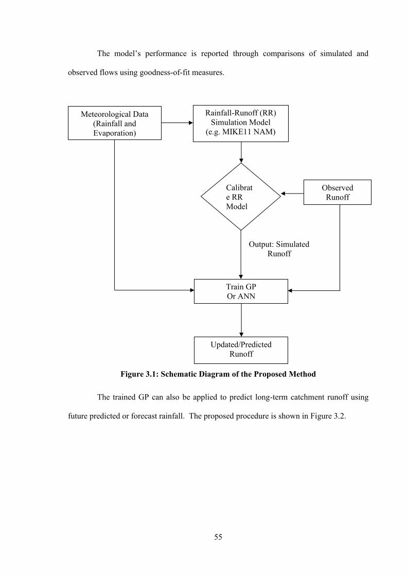
55

The model’s performance is reported through comparisons of simulated and

observed flows using goodness-of-fit measures.

Figure 3.1: Schematic Diagram of the Proposed Method

The trained GP can also be applied to predict long-term catchment runoff using

future predicted or forecast rainfall. The proposed procedure is shown in Figure 3.2.

Rainfall-Runoff (RR) Simulation Model

(e.g. MIKE11 NAM)

Train GP Or ANN

Output: Simulated Runoff

Updated/Predicted Runoff

Meteorological Data (Rainfall and Evaporation)

Calibrate RR Model

Observed Runoff

56

Figure 3.2: Long term Runoff Prediction

3.3. Application

GP and ANN are applied for forecasting of Duckmaloi Weir Inflows. Duckmaloi

Weir is located on Duckmaloi River (see Figure 3.3), adjacent to the eastern side of Oberon

Dam catchment, Australia. The catchment area at the weir is approximately 112 km2 and

storage capacity 20 ML (DNR, 2007). A Sacramento model was built and calibrated by

DNR. The results from proposed method will be compared against Sacramento results.

Firstly, the aim of this study is to develop relationship between the future inflow at

the Duckmaloi catchment outlet using rainfall and runoff data available up to the current

time t. Mathematically, the relationship can be expressed:

),.....,,,....,( tmtttttmtttttnt QQQRRRfQ −−−−+ = (1)

Long Term Rainfall Generated form

GCM/Rainfall Scenarios

Update Runoff using Trained GP/ANN

Output: Simulated NAM Runoff

Long Term Runoff

Rerun RR Model

57

Where, Q is the inflow (m3/s), R is the rainfall intensity (mm/day), n refers to how

far into the future the inflow prediction is desired, m represents how far back the recorded

data in the time series are affecting the inflow prediction and ∆t is time interval.

Figure 3.3: Oberon Dam and Duckmaloi Weir Catchments

The performance of the model results is reported through the comparisons of

simulated and observed flows using two goodness-of-fit measures. They are coefficient of

determination and coefficient of efficiency.

Coefficient of Determination: Coefficient of determination (R2) is defined as the

squared value of the coefficient of correlation which is calculated as:

2

1

2

1

2

12

)()(

))((

−−

−−

=

==

=

n

ii

n

ii

n

iii

PPOO

PPOOR (2)

Where, O observed, and P predicted values.

58

R2 estimates the combined dispersion against the single dispersion of the observed

and predicted series. The range of R2 lies between 0 and 1 which describes how much of the

observed dispersion is explained by the prediction. A value of 0 means no correlation at all

whereas a value of 1 means that the dispersion of prediction is equal to that of the

observation.

Coefficient of Efficiency: Coefficient of Efficiency (E) proposed by Nash and

Sutcliffe (1970) is defined as one minus the sum of the absolute squared differences between

the predicted and observed values normalized by the variance of the observed values during

the period under investigation (Krause, et al., 2005). It is calculated as:

=

=

−

−

−= n

ii

n

iii

OO

POE

1

2

2

1

)(

)(1 (3)

The range of E lies between 1 (perfect fit) and − .

3.3.1. Case Study I

Firstly, an example event is demonstrated with the rainfall and flow data in year

1990. The inflow forecasting for the Duckmaloi catchment is conducted for 1-day lead-time

prediction. The GP and ANN are trained with the input data set containing variables of

rainfall and inflow at current time and the value of n is set to 1 (see eq. 1). In these models,

fifty percent of the data was used for training and fifty percent for validation. The GP and

ANN results are presented in Figure 3.4 and Figure 3.5 respectively. Both models produce

very good prediction of Duckmaloi Weir inflows. The goodness-of-fit measure is presented

in Table 3. 1. Visually, GP produces better prediction than ANN especially during recession.

Figure 3.5 shows some noise in the prediction at the tail of the hydrograph. GP usually

59

derives physical relationship between the variables. A series of relationships are produced

by GP. However, only one is shown below.

𝑄𝑡+∆𝑡 = 𝑅𝑡+∆𝑡 + 𝑄𝑡 − 0.0776213 ∗ 𝑄𝑡−∆𝑡 (4)

Where, 𝑄𝑡is discharge at current time, 𝑄𝑡+∆𝑡 is discharge at future time, 𝑅𝑡 is

rainfall at current time and ∆𝑡 is time interval.

Figure 3.4: Comparison of Hydrograph between Observed and GP Runoff – Year 1990

Table 3. 1 Goodness-of-fit measures - 1990

Parameter Genetic Programming

ANN

Coefficient of Determination (R2) 0.88 0.87 Coefficient of Efficiency (E) 0.88 0.87

60

Figure 3.5: Comparison of Hydrograph between Observed and ANN Runoff – Year

1990

3.3.2. Case Study II

In this example, GP and ANN are trained again with whole series of rainfall and

runoff data as used in fish river water supply scheme IQQM modelling report (DNR, 2007).

The data contain time series from 11/10/1954 to 19/02/1981. The comparison of measured

and simulation Duckmaloi Weir inflows are presented in Figure 3.6 and Figure 3.7

respectively. GP performs slightly better than ANN and the coefficient of determination is

found to be 0.73 (see Table 3. 2) which implies very good prediction for long term time

series.

Table 3. 2 Goodness-of-fit measures – 1954 to 1981

Parameter Genetic Programming

ANN

Coefficient of Determination (R2) 0.73 0.71 Coefficient of Efficiency (E) 0.73 0.71

61

Figure 3.6: Comparison of Measured and Simulated Inflows at Duckmaloi Weir - GP

Figure 3.7: Comparison of Measured and Simulated Inflows at Duckmaloi Weir –

ANN

62

3.3.3. Comparison of GP and Sacramento Model Results

Comparison of observed and simulated discharges from Genetic Programming and

Sacramento models are presented in Figure 3.8 to Figure 3.15. Almost all the figures show

that Sacrament model either over-predicted or under-predicted at and around the peak

discharge. Figure 3.16 shows a comparison for an event from June 1960 to October 1960. It

has been found that GP is following the observed discharges especially during the recession

part reasonably well compared to Sacramento model. Yearly volumes of inflows to

Duckmaloi Weir are calculated and plotted in Figure 3.17. Figure 3.17 presents that

Sacramento model under-predicted in 1960, 1971 and 1972 and over-predicted in 1963,

1967, 1968 and 1980.

Figure 3.8: Comparison of Observed and Simulated Discharges from GP and Sacramento Models – 1954 to 1956

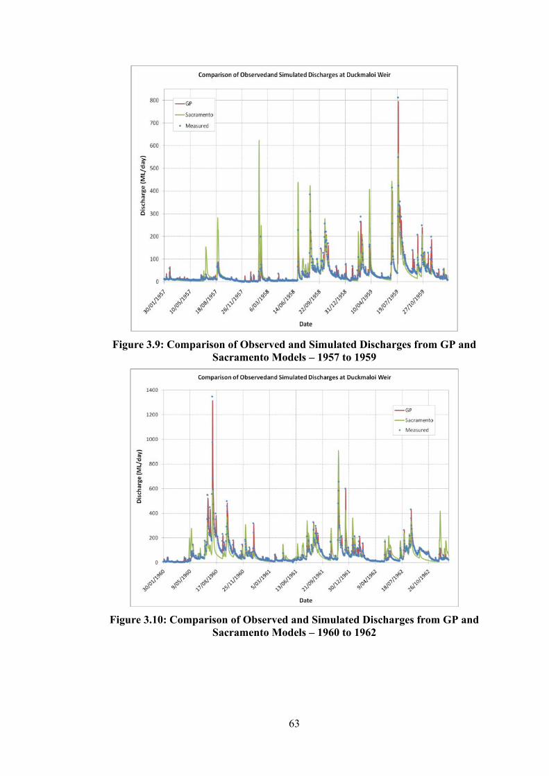
63

Figure 3.9: Comparison of Observed and Simulated Discharges from GP and

Sacramento Models – 1957 to 1959



64





65



66




Sacramento Models – June to October 1960

67

Figure 3.17: Comparison of Observed and Simulated Yearly Volumes of Inflows at

Duckmaloi Weir

To measure the model performance, a low flow event is selected. Figure 3.17 shows

the total volume of inflows to the Duckmaloi Weir were very low in 1965. The corresponding

inflow series is depicted in Figure 3.18. The goodness-of-fit measures for the GP and

Sacramento models are estimated for this particular low flow series and presented in Table

3. 3. Table 3. 3 shows that the coefficient of determination is similar from both model but

the coefficient of efficiency for GP is close to 1 which means that the performance of GP is

reasonable. The flow frequency curves from GP model results and observed flows is shown

in Figure 3. 19. This is also reflected in scatter plot in Figure 3.20 which shows that majority

of GP predicted flows lies around 45 degree line compared Sacramento flows.

Table 3. 3: Model Performance Criteria

Performance Criteria GP Sacramento Coefficient of Determination (R2) 0.80 0.83 Coefficient of Efficiency (E) 0.78 -1.18

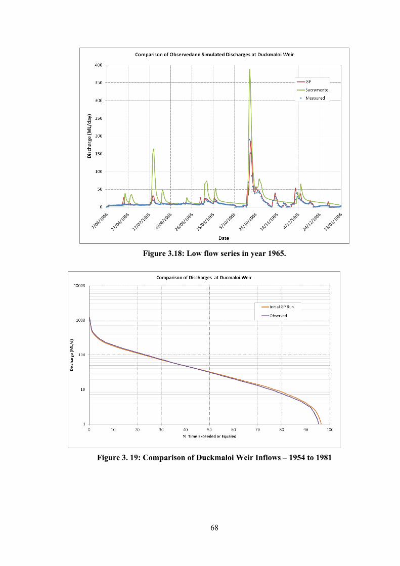
68

Figure 3.18: Low flow series in year 1965.

Figure 3. 19: Comparison of Duckmaloi Weir Inflows – 1954 to 1981

69

Figure 3.20: Scatter Plot of Observed and Simulated Discharges – 1965

3.4. Improvement of Model Calibration using GP

GP model was built using the lagged observed flows as an input. However, GP

automatically discards input variables (lagged flows) that has less influence on the output.

The lagged inflow on the previous day determined by GP has significant influence on the

model prediction. The drawback of this model is that the model input is dependent on the

catchment runoff observed on the previous day which may be erroneous or not available.

The model also cannot be applied for long term simulation as the observed data is not

available. Nonetheless, this can be overcome by using a hybrid approach where the runoff is

generated by a traditional hydrological model which is subsequently used as an input to GP

as a substitute for observed lagged flow. An attempt is made in this research to apply a

conceptual rainfall-runoff model to generate the series of discharges from rainfall and

evaporation data. In this analysis, a MIKE11-NAM model (DHI, 2013) is considered.

70

NAM model was built with the same rainfall as used in section 3.3.2 and the

evaporation data as shown in Figure 3.21. The model was developed with the NAM

parameters as given in Table 3. 4. In this hybrid approach, the MIKE11-NAM parameters

were initially fine-tuned. The model was calibrated with NAM’s “autocalibration”

functionality between the period of 11/10/1954 and 19/02/1981. The initial and updated

NAM parameters are shown in Table 3. 4. The performance of NAM is shown graphically

in Figure 3. 22 in terms of ranked plot. The coefficient of determination from this model was

found to be 0.78.

Figure 3.21: Evaporation Time Series

NAM predicted flow was then used as inflow to improve the calibration using GP.

The initial GP model was developed using the input of rainfall and the NAM predicted flow

to predict the observed flow. The GP model is shown below (see equation 5). The flow

duration curve is shown in Figure 3.23. Figure 3.23 demonstrates that GP has significantly

improved model calibration especially flow under 40 ML/day. The performance of GP is

71

also improved further by including the base flow (see Figure 3.23). The corresponding

derived relationship from GP is shown equation 6. The model accuracies in terms of R2 are

shown in Table 3. 5. GP with model base flow component performed better (Figure 3.23)

than and NAM and GP without the base flow.

Qgp = 0.6534*Qnam + 0.00526*R*Qnam - 0.4636*SIN(0.6534*Qnam) (5)

Qgp = 0.7155*BF + 0.4908*Qnam*BF + 0.007869*R*Qnam (6)

Where, Qgp = Predicted flow by GP; Qnam = Predicted flow by NAM; R = Rainfall; BF = Base Flow

Figure 3. 22: Ranked Plot - Comparison of Duckmaloi Weir Inflows

72

Table 3. 4: NAM Model Parameters

Parameter Initial Value Calibrated

Value Unit

Maximum Water Content in Surface Storage (Umax)

19.6 19.38 mm

Maximum Water Content in Root Zone Storage (Lmax)

300 297.25 mm

Overland Flow Runoff Coefficient (CQOF) 0.124 0.12 - Time Constant for Routing Interflow (CKIF) 778.1 805.61 hour Time Constant for Routing Overland Flow (CK1)

22.9 25.68 hour

Root Zone Threshold Value for Overland Flow (TOF)

0.64 0.61 -

Root Zone Threshold Value for Interflow (TIF)

0.935 0.86 -

Root Zone Threshold Value for GW Recharge (TG)

0.925 0.96 -

Time Constant for Routing Baseflow (CKBF) 3833 3718.64 hour

Table 3. 5: Mode Performance – GP vs. NAM

Model Coefficient of Determination (R2) NAM 0.78 GP Without BF 0.81 GP with BF 0.82

Figure 3.23: Ranked Plot of Daily Recorded and Modelled Inflow to Duckmaloi Weir Improvement by Base Flow

1

10

100

1000

10000

0 0.2 0.4 0.6 0.8 1

Dis

char

ge (

ML/

day

)

% of Exceedance Probability

Comparison of Discharges - NAM and GP Vs Observed

NAMGP with BFGP Without BFObserved

73

3.5. Long Term Rainfall Scenario Analysis

This analysis required long term (100 year) inflow and rainfall time series (1890-

2006) which were collected from NSW State Water Corporation (DNR, 2007). From this

long term rainfall series, two future climatic scenarios (assumed two hypothetical rainfall

time series) were generated using the following procedures before feeding the data to GP

model as described in the previous section. These two rainfall scenarios have been developed

to analyse the affect rainfall variation on the catchment flow. These analyses will provide

some likely scenarios and useful information to water manager for planning and

management of the catchment.

3.5.1. Scenario 1: Stretching the Minimum Rainfall Duration in Sequence

(Stretched rainfall)

In this scenario, the dry period is extended by assuming the low rainfall over the

five years in last 100 years will continue for next 10 years. The step-by-step procedures are

described below:

Yearly total rainfalls are estimated from last more than 100 year rainfall series

starting from 1901 to 2006, (Figure 3. 24). It can be seen in Figure 3. 24 that a five

year spell of minimum total rainfall occurred from 1936 to 1940.

In the next step, five years total rainfall series were calculated. The five year total

rainfall values were sorted in ascending order which shows that the first three

minimum five yearly rainfalls occurred in 1936-1940, 1906-1910 and 1901-1905.

These three five year periods are considered the worst drought sequence in last 100

years.

A future time series was generated assuming the drought could be worse than what

74

had happened historically. With this assumption, these drought sequences are placed

one after another.

The rainfall in 1936-40 remained unchanged but the rainfall in 1941-1945 was

replaced by that in 1906-1910 and 1946-1950 by 1901-1905. The other five yearly

total rainfalls were reshuffled randomly. The original and future stretched five yearly

rainfall (drought) series are presented in Figure 3. 25.

The new five yearly total rainfalls series were distributed back to daily rainfall using

the same temporal pattern as in the original time series.

The initial estimates of flows were generated using MIKE11-NAM.

The GP was run to update the flows.

Figure 3. 24: Yearly Total Rainfall in the Past 100 Years

75

Figure 3. 25: Original and stretched rainfalls - Scenario 1. The x axis label is the year ending of the 5 year period.

3.5.2. Scenario 2: Rainfall Variation

In this scenario, instead of extending the dry period, the rainfall during dry period

is decreased and the rainfall in wet period is increased by a certain percentage. The step-by-

step procedure is described below:

1. The total rainfall over five consecutive years was calculated in a manner similar to

steps 1 and 2 of Scenario 1.

2. Rainfall totals above the average were increased by 20% and rainfall totals below

average declined by 20%. The present and adapted five year total rainfalls are

presented in Figure 3. 26.

3. The new five yearly total rainfalls series were distributed back to daily rainfall using

the same temporal pattern as in the original time series.

4. The initial estimates of flows were generated using MIKE11-NAM.

5. The GP was run to update the flows.

76

Figure 3. 26: Original and Varied Rainfalls – Scenario 2

Figure 3. 27: GP Flow from Stretched Rainfall (Scenario 1)

77

Figure 3. 28: GP Flow from Rainfall Changes (Scenario 2)

3.5.3. Rainfall Scenario Results

The calibrated NAM model was applied to determine initial estimates of 100 year

inflows at the Duckmaloi Weir for both rainfall scenarios. The 100 year flows generated are

shown in Figure 3. 27 and Figure 3. 28 respectively. The inflows were updated using the GP

model as described in equation 5. The results (estimated flow) in terms of ranked plots are

shown in Figure 3. 29. Figure 3. 30 illustrates the corresponding yearly volume. Figure 3.

29 shows that how both scenarios decrease yields at the Duckmaloi Weir if the drought

condition persists. The catchment flows yield below 135 ML/d (86 ML/d for Scenario 1 and

132 ML/d for Scenario 2) for 90% of the time (see Table 3. 6). Table 3. 6 describes how

catchment yields will change if the future climatic scenarios (Scenario 1 and Scenario 2)

vary compared to last 100 year rainfall condition. Scenario 1 and 2 intersects at discharge of

30 ML/d (Figure 3. 29) for the percentage of time exceeded or equalled of 30% (seeTable 3.

6). After this point, the discharge to the Duckmaloi Weir decreases sharply compared to

78

scenario 1 due to the impact of 20% decrease in rainfall. Scenario 2 results also show that

30% of the time there would be no flow to the dam catchment. If the future climatic condition

follows Scenario 2, alternative source of water supply needs to be identified.

The scenario testing demonstrates how this method could be used for making future

water resources management plans under different climate scenarios and contribute to

decisions concerning water supply from alternative sources.

Figure 3. 29: Ranked Plot of 100 years Daily Inflows to Duckmaloi Weir for Scenarios 1 (Stretched Rainfall) and 2 (Rainfall Variation)

79

Figure 3. 30: Yearly Volume of 100 Year Inflows to Duckmaloi Weir for Different

Scenarios 1 (Stretched Rainfall) and 2 (Rainfall Variation).

Table 3. 6: Discharge against % of Time Exceeded or Equaled

% Time Exceeded or Equalled

Discharge (ML/d) Estimated Flow Scenario 1 Scenario 2

1 449 343 465 5 213 139 219 10 135 86 132 30 41 30 31 50 17 13 3 70 7 5 0

3.6. Discussion

This study demonstrates the application of GP for predicting real-time inflows to a

dam catchment, named Duckmaloi Weir. In the first example, the GP model performed well

when one day lagged flow was used for training and validation. In the second example, the

lagged observed flows were replaced with the runoff generated from a traditional calibrated

hydrological model (MIKE11-NAM). The output from NAM was improved by training GP

80

together with the rainfall data. The final calibrated results from GP indicated excellent

agreement between the observed and simulated flows (e.g. R2>0.8). This methodology of

using hybrid model is more versatile and is better suited for the following reasons:

• historical observed flow may be erroneous, and parts of the time series may be

missing;

• more suitable for long-term forecasting (e.g. 100 year); and

• more suitable for real-time prediction as the 1-day lagged data is often not available.

Finally, two examples of long-term climatic scenarios were applied to predict the

possible future 100 year water inflows to Duckmaloi Weir under extreme and extended

drought conditions using flows from the NAM model (second example). The application of

AI (e.g. GP) to improve runoff generated from a traditional conceptual hydrological model

for a real catchment and future possible rainfall scenarios analysis, will provide an

alternative solution to water manger. These example rainfall scenarios are hypothetical but

can be more appropriately replaced by other more relevant scenarios. For example,

downscaled rainfall from the climatic model can be used to assess the impact of climate

change on catchment runoff and dam operation. The analysis demonstrates how it can be

useful for planning future water resource management and decision-making in a dam

catchment.

3.7. Summary

In this chapter, application of Genetic Programming (GP) and Artificial Neural

Network (ANN) have been demonstrated in predicting flow using the rainfall and past

historical observed lagged flow for Duckmaloi Weir catchment located in Oberon, Australia.

GP performed well compared to ANN. The performance of GP was also compared against

traditional Sacramento model and GP’s results were superior.

81

Two examples showing one-day lead prediction solely using GP and another

showing a hybrid approach with MIKE11-NAM and GP reveal some promising results. For

1-day prediction, the GP model demonstrated a closer agreement between observed and

modelled flows with current rainfall and lagged flows. The hybrid model was applied to

update flow prediction from MIKE11-NAM. This approach is useful when measured or

gauged flows are not complete or missing and it is also suitable for long-term prediction.

The 100 year flows were predicted assuming two hypothetical rainfall time series. The

results from this hypothetical rainfall analysis show how the flow conditions vary in the dam

catchment in drought conditions. The analysis provides some information to water manager

about the potential application of hydroinformatics tools (GP, MIKE11-NAM and GP hybrid

models) in the operation and management of water resources.

82

CHAPTER 4

PREDICTION OF HYDROLOGICAL TIME-SERIES USING EXTREME LEARNING

MACHINE (ELM)

This chapter includes the major part of • Atiquzzaman, M. and Kandasamy, J. (2016). “Prediction of Hydrological Time-

Series using Extreme Learning Machine”, Journal of Hydroinformatics. 18.2, pp.345-353, http://dx.doi.org/10.2166/hydro.2015.020.

83

4. Prediction of Hydrological Time-Series Using Extreme Learning Machine (ELM)

4.1. Introduction

The application of data-driven modelling approaches including Artificial Neural

Network (ANN) and Support Vector Machine (SVM) has been widespread in the water

resource engineering field, especially for predicting hydrological time-series. This is because

they can establish complex non-linear relationships between input and output variables

(Tokar and Johnson., 1999). The main advantage of these techniques is that they do not

require the information about the complex nature of the underlying hydrological process.

When data-driven modeling is applied, input variables including precipitation, lagged

precipitation, and lagged discharges are normally employed to forecast the discharges

(Akhtar et al., 2009). Many of these data-driven modelling methods including ANN, ANFIS

and SVM are slow requiring numerous iterations to generate optimal solutions (Ding et al.,

2015 and Zhang et al., 2007), and may not be suitable for real-time prediction where quick

response is vital. Huang et al. (2006) reported that applying typical feed-forward neural

network has been limited due to the use of conventional gradient-based slow learning

algorithms in training and iterative determination of network parameters. To overcome the

long computational time and to produce generalized solution, a learning algorithm called

Extreme Learning Machine (ELM), developed by Huang et al. (2006) was used in this study.

The performance of ELM was compared with conventional NN and SVM on benchmarking

problems in the function approximation and classification areas. Huang et al. (2006) found

that ELM approximates any continuous function and implements any classification. ELM

may need more hidden nodes but learns faster than SVM. The generalization performance

of ELM is stable with a wide range of number of hidden nodes.

Ding et al. (2015) stated that ELM, which requires a single iteration, overcomes the

84

slow training speed and over-fitting problems unlike other conventional ANN learning

algorithm. ELM’s robustness and fast learning rate was proved in different fields including

real dataset classification and regression (Huang et al., 2012). Zhang et al. (2007) applied

ELM to multi-category classification problems in cancer diagnosis and found that ELM did

not have problems like falling in local minima and over-fitting which are commonly

experienced by iteration based learning methods.

This study demonstrates that the method partly overcomes the slow learning issue

by using Extreme Learning Machine (ELM) which predicts the hydrological time-series very

quickly. ELM, which is also called single-hidden layer feed-forward neural networks

(SLFNs), is able to well generalize the performance for extremely complex problems. ELM

randomly chooses a single hidden layer and analytically determines the weights to predict

the output (Huang et al., 2006).

The application of ELM uses a MATLAB program developed for predicting

hydrological flow time-series. The ELM method was applied to predict hydrological flow

series for the Tryggevælde Catchment, Denmark and for the Mississippi River at Vicksburg,

USA. The results confirmed that ELM’s performance was similar or better in terms of Root

Mean Square Error (RMSE) and Normalized Root Mean Square Error (NRMSE) compared

to ANN and other previously published techniques, namely Evolutionary Computation

based Support Vector Machine (EC-SVM), Standard Chaotic Approach and Inverse

Approach (Yu et al., 2004).

4.2. Application

ELM is applied to estimate the catchment runoff. ELM is an AI technique where

the input weights and hidden layer biases are randomly chosen and the output weights are

determined analytically (Huang et al., 2006). ELM generates the parameters associated with

85

hidden nodes without depending on training data. However, ELM transforms the training of

Feed-Forward Neural Network into a linear problem where only connections with output

neurons are adjusted to generate the solutions. Unlike ANN, ELM does not require complex

network architecture to obtain good results. ELM uses three fixed layers i.e. input, hidden

and output layers. In these layers, the number of input variables (flows), the number of nodes

in hidden layers and the activation function (sigmoid function) in output layer need to be

defined beforehand. ELM’s learning speed is extremely fast compared to other machine

learning techniques (e.g. SVM) as it avoids iterative tuning to determine the weights (Huang

et al., 2006 and Huang et al., 2012). Other advantages of ELM can be found in Huang et al.

(2006).

In this study, ELM was applied to predict runoff (one-step-ahead prediction) using

the past and current information of hydrological flows as input data. Mathematically, the

relationship can be expressed as:

),.....,( tmtttttt QQQfQ −−+ = (1)

if past historical flow series is considered.

Or, ),...,..,.....,( tmtttttmtttttt dQdQdQQQQfQ −−−−+ = (2)

if past historical flow and flow difference data series are considered.

Or, ),.....,( tmtttttt dQdQdQfdQ −−+ = (3)

if past historical flow difference series is considered.

where, Q is the flow (m3/s), ttdQ + is error predictor, tttt QQdQ −= +, m represents

how far back the recorded data of the time-series affects the flow prediction and ∆t is time

interval.

Once the error predictor is determined from the model in equation (3), the predicted flow is

estimated as:

86

tttt dQQQ +=+ (4)

The performance of trained ELM was evaluated with standard goodness-of-fit

measures such as Root Mean Square Error (RMSE) and Normalized Root Mean Square Error

(NRMSE).

The RMSE and NRMSE are defined as:

RMSE = √1

𝑁∑ [(𝑄𝑚)𝑡 − (𝑄𝑜)𝑡]2𝑁

𝑡=1 (5)

NRMSE = √∑ [(𝑄𝑚)𝑡 − (𝑄𝑜)𝑡]2/ ∑ [(𝑄𝑜)𝑡 − 𝑄_

𝑜]2𝑁𝑡=1

𝑁𝑡=1 (6)

where (Qm)t and (Qo)t are the predicted and observed values at time t; N is the

number of observations and oQ_

is the mean observed flow.

RMSE represents the forecasting error and estimates the sample standard deviation

of the differences between predicted values and observed values. It is a good measure when

large model errors are not desirable. The NRMSE normalizes the RMSE and facilitates

comparison between datasets. NRMSE close to zero indicates a perfect match between the

observed and predicted values and greater than one means predictions are inferior to the

constant mean value (Liong et al., 2002).

ELM was used to estimate the one-lead-day prediction of flows for Tryggevælde

Catchment (Denmark) and Mississippi River at Vicksburg. The ELM was trained with the

same data as used in Liong et al. (2002) and Yu et al. (2004) and the results were compared

with Standard Chaos Technique, Inverse Approach, ANN and EC-SVM. In Yu et al. (2004),

data in the period 1975-1991 was used for training and 1992-1993 for validation in Standard

Chaos Technique. Phoon et al. (2002) used 1975-1989 for training, 1990-1991 for testing

and 1992-1993 for validation in their application of the Inverse Approach.

87

In this study, data in the period 1975-1991 was used for training and data between

1992-1993 for validation similar to the Standard Chaos Technique. The number of hidden

nodes in ELM was selected as the number of training samples (6204). This is because ELM

can generate zero error when the number of hidden neurons learns the same number of

distinct observations (Huang et al., 2006). For the output node, the widely used sigmoid

activation function was chosen.

4.3. Tryggevælde Catchment

The Tryggevælde Catchment, Denmark (130.5 km2) is located in the eastern part of

Sealand, north of Karise. The catchment is predominantly characterized by clay soil. The

daily measured flows are available for the period 1 January 1975 to 31 December 1993

(Figure 4. 1). The statistics of flow series are: mean flow = 0.977 m3/s; standard

deviation=1.367 m3/s; maximum flow = 11.068 m3/s; and minimum flow = 0.014 m3/s. The

statistics of flows represent that there are distinct wet and dry periods in the time-series.

The training and validation accuracies are presented in Table 4. 1 in terms of RMSE

and NRMSE for ELMI (lagged flow, Q), ELMII (lagged flow difference, dQ) and ELMIII

(Q, dQ). The validation accuracies from all three ELM models were between 0.491-0.504

(RMSE) and 0.337-0.347 (NRMSE) respectively. The ELMIII performed the best amongst

the three models. The time required to train ELM models was about 100sec on a Windows-

based machine (Intel i7 CPU at 2.67GHz). The corresponding validations times were

between 0.47-0.49sec. An ANN model, which estimates the default number of hidden nodes

(81) based on number of input variables, output variables and training samples, was trained

with the same dataset as ELM (hidden nodes = 6204) for approximately 100sec (training

time of ELM) for comparison with ELM. The prediction accuracies of ANN obtained from

633 iterations were 0.588 (RMSE) and 0.403 (NRMSE) (Table 4. 2).

88

Figure 4. 1: Daily Observed Flows at Tryggevælde Catchment (Source: Yu et al.,

2004) Table 4. 1: ELM Prediction Accuracy for both Training and Validation Dataset for

Tryggevælde Catchment

Model No. of Iterations

Training Validation RMSE NRMSE Time (s)

RMSE NRMSE Time (s)

ELMI(Q) Single 0.495 0.362 99.28 0.497 0.341 0.49 ELMII(dQ) Single 0.508 0.372 108.09 0.504 0.347 0.47

ELMIII(Q, dQ) Single 0.488 0.357 100.88 0.491 0.337 0.48

Table 4. 2 compares the ELM results with other available techniques (Liong et al.,

2002; Yu et al., 2004). Yu et al. (2004) used two types of input time-series, namely daily

flow series (Q) and flow difference series (dQ) separately in EC-SVM. The use of dQ-series

in EC-SVM provided better results than the Q-series. The number of iterations required was

151,668 for EC-SVM(Q) and 11,800 for EC-SVM(dQ). All ELM techniques were faster as

no additional iteration was required and produced better results (Table 4. 2). The ELMIII

model improved the prediction accuracy in terms of RMSE by 24% over the standard chaotic

0

2

4

6

8

10

12Fl

ow

s (m

3/s

)

Time (days)

Daily Observed Flows - Tryggevælde Catchment

89

approach, 7% over the Inverse Approach and 4% over the EC-SVM(Q). ELMI performed

similarly.

Table 4. 2: Prediction Accuracy for Validation Dataset, the Number of Iterations and Training Time from Various Techniques for Tryggevælde Catchment

Model RMSE NRMSE No. of Iterations (Training)

Training Time (sec)

Standard Chaos Technique*

0.647 0.444 - -

Inverse Approach* 0.527 0.361 - - EC-SVM(Q)* 0.514 0.352 151,668 -

EC-SVM(dQ) * 0.504 0.347 11,800 - ANN 0.588 0.403 633 100**

ELMI(Q) 0.497 0.341 Single 99.28** ELMII(dQ) 0.504 0.347 Single 108.09**

ELMIII(Q, dQ) 0.491 0.337 Single 100.88** *Liong et al. (2002) and Yu et al. (2004); **Windows Intel i7 at 2.67 GHz

4.4. Mississippi River at Vicksburg Flow

A similar approach, as applied in Section 4.3, was also applied to predict flows in

the Mississippi River at Vicksburg, USA and used the same daily flows documented in Yu

et al. (2004). The Mississippi River basin covers more than 3,220,000 km2 including

tributaries from central USA and two Canadian provinces. The daily measured flows cover

the period 1 January 1975 to 31 December 1993 (Figure 4. 2). The statistics of flow series

are: mean flow = 18,457 m3/s; standard deviation=9,727.27 m3/s; maximum flow = 52,103

m3/s; and minimum flow = 3,908 m3/s.

Table 4. 3 shows that the results of training and validation obtained from ELMI(Q),

ELMII(dQ) and ELMIII(Q, dQ). The time required to train ELM models was about 97sec

on the same computer (Windows Intel i7 CPU at 2.67 GHz). The corresponding validation

times were between 0.45-0.47sec.

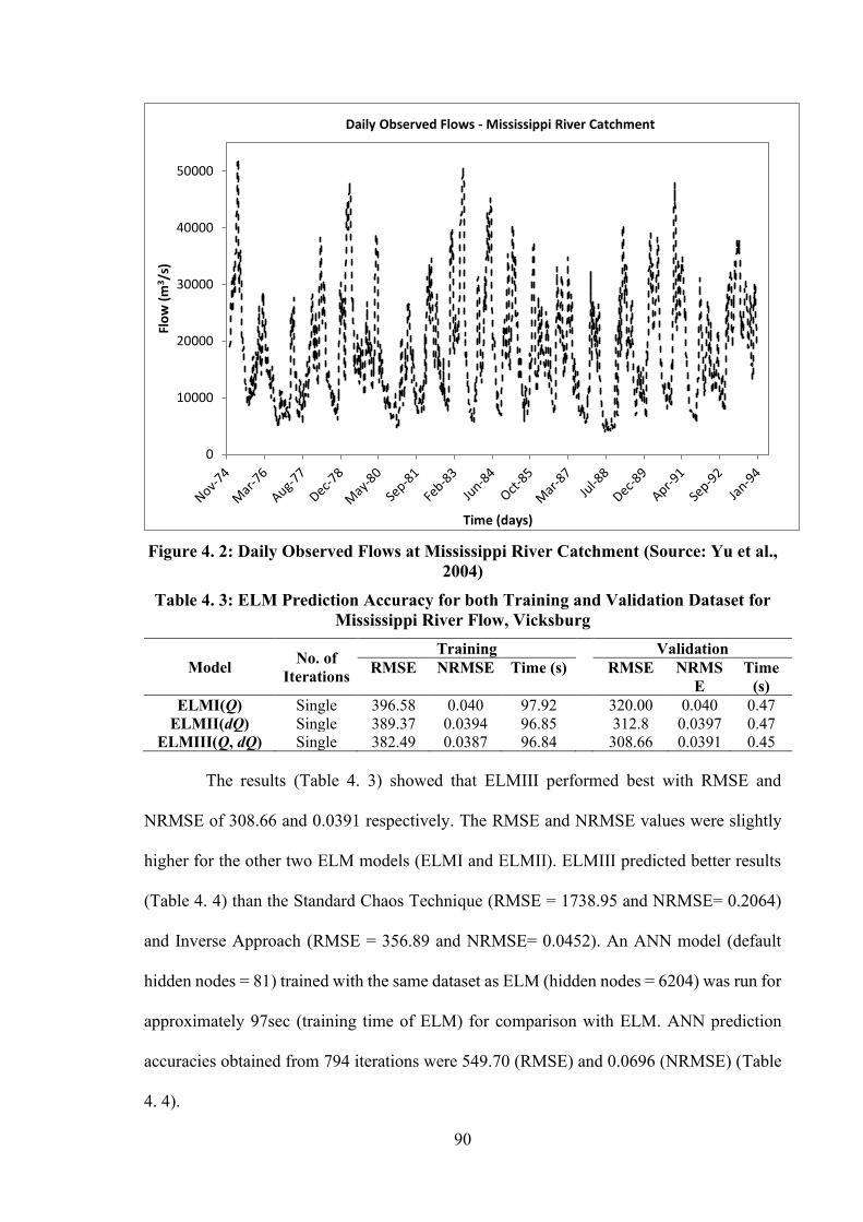
90

Figure 4. 2: Daily Observed Flows at Mississippi River Catchment (Source: Yu et al., 2004)

Table 4. 3: ELM Prediction Accuracy for both Training and Validation Dataset for Mississippi River Flow, Vicksburg

Model No. of Iterations

Training Validation RMSE NRMSE Time (s) RMSE NRMS

E Time

(s) ELMI(Q) Single 396.58 0.040 97.92 320.00 0.040 0.47

ELMII(dQ) Single 389.37 0.0394 96.85 312.8 0.0397 0.47 ELMIII(Q, dQ) Single 382.49 0.0387 96.84 308.66 0.0391 0.45

The results (Table 4. 3) showed that ELMIII performed best with RMSE and

NRMSE of 308.66 and 0.0391 respectively. The RMSE and NRMSE values were slightly

higher for the other two ELM models (ELMI and ELMII). ELMIII predicted better results

(Table 4. 4) than the Standard Chaos Technique (RMSE = 1738.95 and NRMSE= 0.2064)

and Inverse Approach (RMSE = 356.89 and NRMSE= 0.0452). An ANN model (default

hidden nodes = 81) trained with the same dataset as ELM (hidden nodes = 6204) was run for

approximately 97sec (training time of ELM) for comparison with ELM. ANN prediction

accuracies obtained from 794 iterations were 549.70 (RMSE) and 0.0696 (NRMSE) (Table

4. 4).

0

10000

20000

30000

40000

50000Fl

ow

(m

3 /s)

Time (days)

Daily Observed Flows - Mississippi River Catchment

91

Table 4. 4: Prediction Accuracy for Validation Dataset, the Number of Iterations and Training Time from Various Techniques for Mississippi River Flow, Vicksburg

Model RMSE NRMSE No. of Iterations (Training)

Training Time (sec)

Standard Chaos Technique*

1738.95 0.2064 - -

Inverse Approach* 356.89 0.0452 - - EC-SVM(Q)* 306.58 0.0387 1,732.579 -

EC-SVM(dQ) * 304.26 0.0385 47, 590 - ANN 549.70 0.0696 794 97**

ELMI(Q) 320.00 0.04 Single 97.92** ELMII(dQ) 312.8 0.0397 Single 96.85**

ELMIII(Q, dQ) 308.66 0.0391 Single 96.84** * Liong et al. (2002) and Yu et al. (2004); **Windows Intel i7 at 2.67 GHz

Table 4. 4 shows that the RMSE and NRMSE of ELM models were slightly higher

compared to EC-SVM(Q) and EC-SVM(Q, dQ) models. However, ELM predicted these

solutions quickly (single run) compared to EC-SVM(Q) and EC-SVM(Q, dQ), where

1,732,579 and 57,590 iterations, respectively were required. This demonstrates that ELM

can be efficient for online and real-time applications.

4.5. Discussion

This study demonstrates the application of a new AI technique, called ELM for the

prediction hydrological flow time-series from Tryggevælde and Mississippi River

Catchment. The data obtained from a relatively small (Tryggevælde Catchment, Denmark)

and large catchment (the Mississippi River Catchment at Vicksburg) covered both dry and

wet periods. ELM was not applied to the field of catchment hydrology before and these two

catchments were selected from the literature for comparison purpose. Three different ELM

models considering observed lagged flow (ELM1), flow difference (ELMII) and

combination of these two variables (ELMIII) were built. The results for Tryggevælde

Catchment show that ELMIII (RMSE of 0.491) performed better than ELMI (RMSE of

0.497) and ELMII (RMSE of 0.504) models. Similarly, for Mississippi River Catchment,

ELMIII (RMSE of 308.66) improved the accuracy compared to ELMI (RMSE of 320.00)

92

and ELMII (RMSE of 312.8) models. The prediction accuracies of ELMIII were also similar

or better than ANN and other previously published techniques including EC-SVM, Standard

Chaotic Approach and Inverse Approach. More specifically, ELMIII improved the flow

prediction accuracy in terms of RMSE by 24% over Standard Chaos Technique, 7% over

the Inverse Approach and 4% over the EC-SVM for the Tryggevælde Catchment. ELM

provided solutions of similar accuracy to EC-SVM when predicting Mississippi River flows.

ELM’s reached the solutions quickly compared to other techniques including EC-

SVM. This is because no additional iteration is required in ELM whereas other techniques

require thousands of iterations to predict the same flow time-series although most do so with

less accuracy. Such runs typically have a much longer processing time. Importantly, this

processing time will significantly increase for more complex scenarios where many more

iterations are required to obtain an optimal solution. This longer processing time may be a

limiting factor for real-time application. ELM learns the training dataset very quickly which

means that this method is suitable for flood forecasting, the prediction of inflows for

reservoir operations, supply of water to meet irrigation demand, real time control of water

systems and sewer systems, etc. Furthermore, by having improved or at least comparable

prediction accuracy to other available methods, ELM is no less capable for use in water

resource management and decision-making.

4.6. Summary

ELM was applied to predict hydrological flow time-series for the Tryggevælde

Catchment (Denmark) and Mississippi River at Vicksburg (USA). The results show that

ELM’s performance is reasonable for 1-day lead prediction compared to ANN and other

previously published techniques. The real strength of ELM is the short computational run-

time to reach solutions comparable with other techniques including EC-SVM. ELM’s fast

93

learning capability from a training dataset means that it would be more suitable for on-line

and real-time applications where quick processing is important or vital. However, the

robustness of ELM’s performance (improved accuracy) on different input parameters, longer

lead day prediction and extrapolation capability was not investigated. The sensitivity of

ELM’s performance on input parameters is thoroughly investigated and reported in Chapter

5 including application to a local catchment.

94

CHAPTER 5

ROBUSTNESS OF EXTREME LEARNING MACHINE (ELM) IN THE PREDICTION OF

HYDROLOGICAL FLOW SERIES

This chapter includes the major part of • Atiquzzaman, M. and Kandasamy, J. (2018). “Robustness of Extreme Learning

Machine in the prediction of hydrological flow series.”, Computers & GeosciencesJournal, 120, pp. 105-114, http://dx.doi.org/10.1016/j.cageo.2018.08.003.

95

5. Robustness of Extreme Learning Machine (ELM) in the Prediction of Hydrological Flow Series

5.1 Introduction

Predicting hydrological flow series generated from a catchment is an important aspect

of water resources management and decision making. The underlying process of prediction of

flows from a catchment is complex and depends on many parameters.

Application of Artificial Intelligence (AI) based machine learning techniques including

Artificial Neural Network, Genetic Programming (GP) and Support Vector Machine (SVM)

replaced the complex modelling process and at the same time improved the prediction accuracy

of hydrological time-series. However, they still require numerous iterations and computational

time to generate optimum solutions.

This study applies the Extreme Learning Machine (ELM) to hydrological flow series

modeling and compares its performance with two most superior techniques GP and Evolutionary

Computation based SVM (EC-SVM) to demonstrate its fast learning capability. Atiquzzaman

and Kandasamy (2016b) demonstrated that ELM’s learning speed and accuracy were comparable

to Standard Chaos Technique, Inverse Approach and EC-SVM in the forecasting of hydrological

time-series. However, the robustness of ELM’s performance on different input parameters,

longer lead day prediction and extrapolation capability was not investigated by Atiquzzaman and

Kandasamy (2016b). This chapter documents the performance of ELM tested with different

combinations of input variables. The robustness of ELM was evaluated by varying number of

lagged input variables, the number of hidden nodes and input parameter (regularization

coefficient). The number of nodes in the hidden layer was varied to check the sensitivity of

ELM’s result. The generalization capability of ELM was investigated for longer lead-day

prediction (e.g. second and third) and for its extrapolation capability. The robustness and

performance of ELM were studied using the data from three different catchments located in three

96

different climatic conditions. ELM was applied to the Tryggevælde (Denmark), Mississippi

River (USA) and Duckmaloi Weir (Australia) Catchments.

The study results described in this chapter show that (1) ELM yields reasonable results

with two or higher lagged input variables (flows) for 1-day lead prediction; (2) ELM produced

satisfactory results very rapidly when the number of hidden nodes was greater than or equal to

1000; (3) ELM showed improved results when regularization coefficient was fine-tuned; (4)

ELM was able to extrapolate extreme values well; (5) ELM generated reasonable results for

higher number of lead days (second and third) predictions; (6) ELM was computationally much

faster and capable of producing better results compared to other leading AI methods for

prediction of flow series from the same catchment. ELM has the potential for forecasting real-

time hydrological flow series.

5.2 Data and Methods

5.2.1 Catchment Data

ELM is capable of producing better flood prediction for any catchment under different

climatic condition. To demonstrate the robustness ELM, data from three different catchments

obtained from three different climatic conditions (Liong et al., 2002 and Yu el al., 2004) was

used in this study and the results were compared with other published techniques.

The first catchment is Tryggevælde Catchment (130.5 km2) located in Denmark in the

eastern part of Sealand, north of the village Karise (Figure 4. 1). This is a small catchment

characterized by clay soil which results in very flashy flow.

The second one is for the Mississippi River catchment in USA. The Mississippi River

is one of the world’s greatest river systems. Both catchments have the daily measured flows for

the period of 1 January 1975 to 31 December 1993 (Figure 4. 1 and Figure 4. 2) (Yu et al., 2004).

The Tryggevælde Catchment is small, and the maximum recorded flow is 11.068 m3/s whereas

97

Mississippi River catchment is very large and the maximum flow is 52,103 m3/s. In this study,

flow data between 1975 to 1991 was used for training ELM and the data between 1992 to1993

for testing. No rainfall and evaporation data were applied as input series.

Location Map (not in Scale) Ducmaloi Weir Catchment

Figure 5. 1: Location of Duckmaloi Weir Catchment

The third catchment used for this analysis is the Duckmaloi Weir catchment which is

located south of Oberon and approximately 180 km west of Sydney, Australia (see Figure 5. 1).

The catchment covers an area of approximately 112 km2 and is drained by Duckmaloi River and

its tributaries. The weir is located on the Duckmaloi River. It provides Oberon with its water

supply and cooling water for Mount Piper and Wallerawang power stations. The operational

capacity of the weir is 20ML at full supply level of RL 1,057.64m AHD. A stream gauging station

is located just downstream of Duckmaloi Weir and has recorded data from 18 October 1954 to

19 February 1981 (Figure 5. 2). The rainfall data recorded at the station (63036) has continuous

records for more than 100 years. The statistics of flow series are: mean flow = 0.862 m3/s;

standard deviation=1.417 m3/s; maximum flow = 36.014 m3/s; and minimum flow = 0.0 m3/s.

The time series is shown in Figure 5. 2 which shows that there are distinct wet and dry periods

in each year. In ELM, rainfall and flow data from 1954 to 1975 are used for training and from

Australia

98

1976 to 1981 for testing.

Figure 5. 2: Daily Observed Flows - Duckmaloi Weir Catchment

5.2.2 Methods

Model: The basic hidden node based ELM (Huang et al., 2006) as described in Chapter

4, has been applied in this analysis. Huang et al. (2012) stated that if the number of hidden

neurons and the number of input samples are equal, ELM can, in theory, approximate the training

of samples with zero error. However, in order to get stable and better generalization performance,

a parameter called the regularization coefficient (C) (see Huang et al., 2012) was introduced in

ELM. The performance of ELM also depends on the activation function. If these are

appropriately selected, ELM does not degrade the generalization capability (Lin et al., 2014).

Modelling Technique: ELM and GP were used to estimate the catchment runoff using

past catchment flow as input data. Mathematically, if only the past historical flow series is

considered, the relationship can be expressed:

0

5

10

15

20

25

30

35

40

Dis

char

ge (

ML/

day

)

Time

Daily Observed Flows - Duckmaloi Weir Catchment

99

),.....,( tmtttttnt QQQfQ −−+ = (1)

if the only past historical flow series is considered.

),.....,,,....,,( tmtttttltttttttnt QQQRRRRfQ −−−−++ = (2)

if the past and present rainfalls and past historical flow series are considered.

where Q is the flow (m3/s), R is the rainfall (mm), n refers to how far into the future

the inflow prediction is desired; l and m represents how far back the recorded time series

(rainfall and flows) affects the flow prediction. ∆t is time interval.

5.2.3 Model Development

Model Architecture: In this study, the dependency of ELM on the lagged input

variables, number of hidden nodes and regularization coefficient (C) were analyzed with sigmoid

activation function to develop the best trained model. The authors selected sigmoid activation

function as this produced best results compared to other activation functions (Atiquzzaman and

Kandasamy, 2016b). The C value is optimized to improve the results.

Lagged Variables: ELM and GP’s performances for one-day lead predictions (n = 1)

were tested by assigning a number of lagged flows (m) as defined in equation 1. Initially, seven

day lagged flows (m = 7) with the number of hidden nodes set to the number of training samples

were applied.

In ELM, m was decreased one-by-one and each time the model was re-run to assess its

performance. The best performing model was used for subsequent analysis.

In GP, an algorithm called Eureqa (Schmidt and Lipson, 2009) was used which

automatically test a range of m in the training phase to produce a model with the m that best

correlates with the output.

Number of Hidden Nodes: The number of the hidden nodes needs to be defined

beforehand. The influence of the number of hidden nodes on the model prediction was analyzed

100

with the best performing model obtained in the manner outlined in the previous section. The

number of hidden nodes applied was varied from 10 to 6204 to test the model performances. The

upper limit was set to 6204 as this equals the total number of training samples according to Huang

et al. (2012) produces best results.

Regularization Coefficient: The performance of ELM depends on the regularization

coefficient (C). The default value of C is 1. The model with an optimized number of hidden nodes

found from previous analysis was chosen to undertake further test to improve the accuracy by

varying the regularization coefficient. The default value was increased by a factor of ten each

time in a series of runs to test the model performances. The factor ten was used to rapidly increase

the C value to quickly access which gave a better solution.

5.2.4 Extrapolation and Higher Lead-Day Prediction

ELM’s ability to extrapolate flows was tested by training it with a dataset that did not

include the maximum values of the entire time-series. In this test, the input data series was split

up into two groups. The portion of the time series which contained the largest discharge was used

as the production dataset. The remaining of the data series was used for training. The trained

model was applied to verify if it could predict the extreme values of the time-series.

The ELM model was also applied for higher lead-days (e.g. n=2, 3, 5) predictions to

access and compare ELM’s performance against other published AI techniques.

5.2.5 Performance Measures

The model prediction accuracies were assessed using four performance measures,

namely Correlation Coefficient (CC), Nash-Sutcliffe Efficiency (NSE), Root Mean Square Error

(RMSE) and Normalized Root Mean Square Error (NRMSE). NSE and RMSE were found to be

the two mostly used performance measures according to a review by Nourani et al. (2014).

101

Rathinasamy et al. (2014) proposed wavelet-based performance measures (Multiscale NSE and

NRMSE) instead of traditional NSE and RMSE as they found that the proposed measures were

more reliable. However, in this study NSE, RMSE and NRMSE were selected primarily to

undertake a direct comparison with the results given in Yu et al. (2004) and Yu and Liong (2007).

It is unlikely that other performance measure will adversely affect the assessment of ELM’s

performance since ELM performed well across the entire range of performance measures tested.

CC provides information on linear dependence between observed and simulated values

(Kisi et al., 2013) and its values lies between 0 and 1. A value of 0 means no correlation at all

whereas a value of 1 means that the dispersion of prediction is equal to that of the observation.

RMSE represents the forecasting error and estimates the sample standard deviation of the

differences between predicted values and observed values. A RMSE value of zero indicates

perfect match whereas higher values represent no match between the observed and modelled

output. It is a good measure when large model errors are not desirable. Another criterion

frequently used in the context of assessing the performance of hydrological models is NSE. The

NSE provides a measure of the model’s ability to predict observed values. In general, high values

of NSE (up to 100%) and small values for RMSE indicate good model predictions.

5.3 Results

5.3.1 Influence of Lagged Variables

The ELM model was run for Tryggevælde and Mississippi River catchments with flow

data as input for different m values ranging from 1 to 7. The number of hidden nodes was set to

the number of training samples (i.e. 6204). The CC, NSE, RMSE and NRMSE values for training

and testing are presented in Table 5. 1 for Tryggevælde and Table 5. 2 for Mississippi River

catchments. The time required to train ELM for the two catchments was less than 122sec. The

CC and NSE are higher than 0.9 and 0.8 respectively for all training and testing results which

102

show that ELM predicts generalized results for all lagged input variables above 1. The RMSE

for Tryggevælde catchment ranged from 0.495 to 0.560 (Figure 5. 3) and NRMSE from 0.339 to

0.384 for testing results. Similarly, for Mississippi River catchment, the RMSE varied from

315.77 to 608.33 (Figure 5. 5) and NRMSE from 0.04 to 0.077 for testing results. The RMSE

values for these two catchments vary as the magnitude of flows are very different (average flow

for Tryggevælde is 0.977 m3/s and 18,457 m3/s for Mississippi River) and the deviations between

observed and predicted flows differ significantly. Though, ELM produced reasonable results for

all runs, the minimum error (e.g. RMSE and NRMSE) for the testing dataset was obtained when

m = 4 (ELM4) for Tryggevælde catchment and m = 2 for Mississippi River catchment (see Table

5. 1). This is because smaller catchment responds quicker to changes in climatic conditions than

bigger catchment. Therefore, more number of lagged variables are required to detect fast

changing flows for accurate prediction. For the larger catchment (Mississippi River catchment),

lagged variables above 2 produced similar results (see Table 5. 2) since catchment response is

very slow. The scatter plots of observed and modelled flows for training and testing datasets are

shown in Figure 5. 4 for Tryggevælde catchment and Figure 5. 6 for Mississippi River catchment.

It shows good agreement between the measured and predicted daily discharge. The measured

and predicted runoffs are evenly scattered around the line of agreement (best fit) especially for

the Mississippi River (Figure 5. 6).

The same data was applied to GP for comparison. Table 5. 1 and Table 5. 2 show the

results of GP for both catchments. GP automatically discards runs of poorer performing lagged

variables and produced a solution where m = 2. The time taken was 202.8sec in 77,082 iterations

for Tryggevælde catchment and 8min 20sec and 181,892 iterations for Mississippi River

catchment. The GP results in terms of RMSE and NRMSE were worse than ELM. As ELM2 and

ELM4 model produced comparable results, ELM4 is used in the subsequent analysis for

consistency with Tryggevælde catchment.

103

Figure 5. 3: ELM Model Prediction Accuracies for Training and Testing Dataset -

Tryggevælde Catchment

(a)

(b)

Figure 5. 4: Scatter Plot of Observed and Predicted Training (a) and Testing (b) Dataset for Tryggevælde Catchment

0.75

0.8

0.85

0.9

0.95

1

1 2 3 4 5 6 7

CC

Lagged Flows

Training Testing

0.7

0.75

0.8

0.85

0.9

0.95

1 2 3 4 5 6 7

NSE

Lagged Flows

Training Testing

0.46

0.48

0.5

0.52

0.54

0.56

0.58

1 2 3 4 5 6 7

RM

SE

Lagged Flows

Training Testing

0.310.320.330.340.350.360.370.380.39

0.4

1 2 3 4 5 6 7

NR

MSE

Lagged Flows

Training Testing

0123456789

10

0 2 4 6 8 10

Pre

dic

ted

Dis

char

ge (

m^3

/s)

Observed Discharge (m^3/s)

0123456789

10

0 2 4 6 8 10

Pre

dic

ted

Dis

char

ge (

m^3

/s)


104

Figure 5. 5: ELM Model Prediction Accuracies for Training and Testing Dataset - Mississippi River Catchment

Table 5. 1: Comparison of Prediction Accuracies for Different Lagged Variables - Tryggevælde Catchment

Model Run m* CC NSE RMSE NRMSE Iterations Training Time

ELM1 Training 1 0.914 0.844 0.553 0.395 Single 99.6sec Testing 0.923 0.852 0.56 0.384


ELM3 Training 3 0.930 0.872 0.501 0.358 Single 99sec Testing 0.939 0.883 0.499 0.342





GP Training 2 0.917 0.835 0.554 0.406 77,082 202.8sec Testing 0.927 0.857 0.551 0.378 m* = no of lagged flows in the input

0.75

0.8

0.85

0.9

0.95

1

1 2 3 4 5 6 7

CC

Lagged Variables

Training Testing

0.7

0.75

0.8

0.85

0.9

0.95

1 2 3 4 5 6 7

NSE

Laged Variables

Training Testing

0

100

200

300

400

500

600

700

1 2 3 4 5 6 7

RM

SE

Lagged Flows

Training Testing

00.010.020.030.040.050.060.070.080.09

1 2 3 4 5 6 7

NR

MSE

Lag Time

Training Testing

105

Table 5. 2: Comparison of Prediction Accuracies for Different Lagged Variables - Mississippi River Catchment

Model Run m* CC NSE RMSE NRMSE Iterations Training Time








GP Training 2 0.999 0.998 414.81 0.042 181,892 8min 20sec Testing 0.999 0.998 321.70 0.041 m* = no of lagged flows in the input

(a) (b)

Figure 5. 6: Scatter Plot of Observed and Predicted Training (a), and Testing Dataset (b) for Mississippi River Catchment

For Duckmaloi Weir catchment, the model is run with flow and rainfall data as input for

different values of l and m with number of hidden nodes of about 7745. Table 5. 3 shows the

predictions accuracies for different combination of l and m. The total time required to train the

ELM model ranges from 3.14min to 3.29min. The CC and NSE are found to be greater than 0.9

and 0.8 respectively for all the runs (see Figure 5. 7). Figure 5. 7 shows that the RMSE from

0

10000

20000

30000

40000

50000

Pre

dic

ted

Dis

char

ge (

m^3

/s)


05000

10000150002000025000300003500040000

0 10000 20000 30000 40000

Pre

dic

ted

Dis

char

ge (

m^3

/s)


106

testing results ranges from 33.099 (ELM2) to 38.235 (ELM3) and NRMSE from 0.284 (ELM2)

to 0.328 (ELM3) (see Figure 5. 7). The RMSE values for this catchment are not the same

compared to the previous two catchments as the difference in observed and predicted flows

differs significantly. ELM produces reasonable solutions for all runs. However, the minimum

error is obtained when l and m values are 2 (see model ELM2) and RMSE and NRMSE are found

to be 33.099 and 0.284. The scatter plot of observed and modelled flows for training and testing

datasets is shown in Figure 5. 8 for Duckmaloi Weir catchment. It shows good agreement

between the measured and predicted daily discharge. The measured and predicted runoffs are

evenly scattered around the line of agreement (best fit).

The comparisons of ELM and GP are presented in Table 5. 3. GP produces optimal

solution based on current rainfall (l=1) and past flow (m = 1) with total number of iterations of

255,473 in 12.52min. The GP results show that CC, NSE, RMSE and NRMSE from testing

results are 0.85, 0.729, 60.715 and 0.52 respectively. However, ELM produced superior results

even with l =1 and m = 1 (see ELM1 in Table 5. 3) where CC, NSE, RMSE and NRMSE are

0.953, 0.907, 35.56 and 0.305 respectively. ELM2 model (Table 5. 3) improves the prediction

accuracy by 45.5% in terms of RMSE and ELM1 by 41.4% compared to GP.

Table 5. 3: Prediction Accuracy for Duckmaloi Weir Catchment Model Run (l, m)* CC NSE RMSE NRMSE Iterations Training Time

(min)

ELM1 Training (1,1) 0.915 0.837 49.742 0.404 Single 3.21 Testing 0.953 0.907 35.560 0.305

ELM2 Training (2, 2) 0.924 0.854 47.124 0.382 Single 3.14 Testing 0.959 0.920 33.099 0.284






GP Training (1, 1) 0.898 0.805 54.402 0.441 255,473 12.52 Testing 0.85 0.729 60.715 0.520 *l = no of lagged rainfall including current rainfall in the input *m = no of lagged flows in the input

107

Figure 5. 7: ELM Model Prediction Accuracies for Training and Testing Dataset - Duckmaloi Weir Catchment

(a) (b)

Figure 5. 8: Scatter Plot of Observed and Predicted Training (a) and Testing (b) Dataset for Duckmaloi Weir Catchment

5.3.2 Influence of Number of Hidden Nodes

ELM4 (m=4) was run for Tryggevælde and Mississippi River Catchment with different

number of hidden nodes to test its influence on the prediction accuracy. The number of hidden

nodes tested ranged from 10 to number of training samples (6204). The results in terms of CC,

0.75

0.8

0.85

0.9

0.95

1

1 2 3 4 5 6 7

CC

Lagged Variables

Training Testing

0.7

0.75

0.8

0.85

0.9

0.95

1 2 3 4 5 6 7

NSE

Laged Variables

Training Testing

0

10

20

30

40

50

60

1 2 3 4 5 6 7

RM

SE

Lagged Variables

Training Testing

0

0.1

0.2

0.3

0.4

0.5

1 2 3 4 5 6 7

NR

MSE

Lagged Variables

Training Testing

05

10152025303540

0 10 20 30 40

Pre

dic

ted

Dis

char

ge (

m^3

/s)


0

5

10

15

20

25

30

35

0 10 20 30

Pre

dic

ted

Dis

char

ge (

m^3

/s)


108

NSE, RMSE and NRMSE for both training and testing are given in Table 5. 4 for Tryggevælde

Catchment and Table 5. 5 for Mississippi River Catchment. The CC and NSE for both catchments

are higher than 0.9 and 0.8 respectively for all runs. The prediction errors in terms of RMSE and

NRMSE decrease with larger number of hidden nodes (see Table 5. 4 and Table 5. 5). The

variations of RMSE with hidden nodes are presented in Figure 5. 9. For Tryggevælde Catchment,

the RMSE and NRMSE values for testing dataset are 0.574 and 0.393 respectively for 10 hidden

nodes (ELM4-1) and 0.495 and 0.339 respectively for 6204 hidden nodes (ELM4).

Table 5. 4: Influence of Number of Hidden Nodes on Prediction Accuracy for Tryggevælde Catchment

No. Model Run

No of Hidde

n Notes

CC NSE RMSE NRMSE Training Time

% RMSE Improvement Compared to 1000 Nodes

1 ELM4-1 Training 10 0.911 0.829 0.566 0.414 <1sec Testing 0.921 0.837 0.574 0.393 -




5 ELM4-5 Training 1000 0.929 0.862 0.507 0.371 3.2sec Testing 0.938 0.869 0.508 0.348 -

6 ELM4-6 Training 2000 0.930 0.865 0.503 0.368 10.9sec Testing 0.939 0.871 0.502 0.343 1.2


8 ELM4-8 Training 5000 0.931 0.867 0.499 0.365 63sec Testing 0.941 0.873 0.496 0.340 2.4


10 ELM4 Training 6204 0.931 0.867 0.498 0.364 99sec Testing 0.941 0.885 0.495 0.339 2.6

109

Figure 5. 9: Influence of Hidden Nodes on ELM Model Accuracy- Tryggevælde Catchment

For Mississippi River Catchment, these values range from 734.51 and 0.093 for 10

nodes to 320.15 and 0.041 for 6204 nodes respectively. The RMSE value decreased by 13.8%

for Tryggevælde Catchment and 56% for the Mississippi River. The time required to train ELM

increased from less than 1s for 10 nodes to less than 104sec for 6204 nodes (Table 5. 4 and Table

5. 5). The percentages of improvement of the models in comparison with 1000 nodes model

(ELM4-4) are shown in last column of Table 5. 4 and Table 5. 5. The number of hidden nodes

of 1000 was chosen for comparison as the accuracy does not improve significantly with nodes

above this number. The maximum improvement of accuracy in terms of RMSE was only 2.6%

for Tryggevælde Catchment and 1.2% for Mississippi River Catchment when the number of

hidden nodes was increased from 1000 to 6204. Figure 5. 10 shows that the RMSE for a big

catchment like the Mississippi River, was less sensitive to increased number of hidden nodes.

Although, the accuracy of ELM did not significantly improve where the number of hidden nodes

was greater than or equal to1000, the training time increased significantly. This suggests that

ELM is capable of producing good solutions very fast with a modest number of hidden nodes

(e.g. 1000). The model with 1000 hidden nodes (ELM4-5) was investigated for these two

0.44

0.46

0.48

0.5

0.52

0.54

0.56

0.58

10 100 200 500 1000 2000 4000 5000 6000 6204

RM

SE

No of Hidden Nodes

Training Testing

110

catchments only to further improve the accuracy by fine tuning the C parameter and compare the

results with EC-SVM.

Figure 5. 10: Influence of Hidden Nodes on ELM4 Model Accuracy for Mississippi River

Catchment Table 5. 5: Influence of Number of Hidden Nodes on Prediction Accuracy for Mississippi

River Flow, Vicksburg

No. Mod

el Run

No of Hidde

n Notes

CC NSE RMSE NRMSE Training

Time


1 ELM4-1

Training 10 0.997 0.993 812.37 0.082 <1sec Testing 0.996 0.991 734.51 0.093 -

2 ELM4-2


3 ELM4-3


4 ELM4-4


5 ELM4-5

Training 1000 0.999 0.998 399.53 0.041 3.2sec - Testing 0.999 0.998 324.07 0.041

6 ELM4-6

Training 2000 0.999 0.998 398.10 0.040 13.2sec 0.7 Testing 0.999 0.998 321.89 0.041

7 ELM4-7


8 ELM4-8


9 ELM4-9


10 ELM4

Training 6204 0.999 0.998 396.55 0.040 104sec 1.2 Testing 0.999 0.998 320.00 0.041

For Duckmaloi Weir catchment, the best model (ELM2) was run for a series of hidden

nodes to understand the influence of hidden nodes on the prediction accuracy. The number of

0

100

200

300

400

500

600

700

800

900

10 100 200 500 1000 2000 4000 5000 6000 6204

RM

SE

No of Hidden Nodes

Training Testing

111

hidden nodes ranges from 10 to 7000. The results in terms of CC, NSE, RMSE and NRMSE and

the ELM training times are in Table 5. 6. Table 5. 6 shows reasonable results for any number of

hidden nodes with the CC and NSE values always greater than 0.9 and 0.8 respectively. ELM

training time requires time less than 1s for 10 nodes to 2.63mins for 7000 nodes. The prediction

accuracies in terms of RMSE decrease with the increase of hidden nodes (see Figure 5. 11). The

RMSE and NRMSE are 50.381 and 0.432 for 10 hidden nodes (ELM2-1) and 33.184 and 0.284

for 7000 hidden nodes (ELM2-9). Table 5. 6 also shows that though the accuracy of ELM is not

significantly improved if the number of hidden nodes is further increased above 4000, the training

time is increased from 50.19s to 2.63min for 7000 nodes to get only 1.9% improvement in terms

of RMSE (see Figure 5. 11 and Table 5. 6). This suggests that ELM is capable of producing

similar solutions very fast with modest number of hidden nodes. However, the higher number

of hidden nodes generally generates slightly less error in terms of RMSE and NRMSE.

Table 5. 6: Influence of Number of Hidden Nodes on Prediction Accuracy for Duckmaloi Weir Catchment

No. Mod

el Run

No of Hidde

n Notes

CC NSE RMSE NRMSE Training

Time


1 ELM2-1


2 ELM2-2


3 ELM2-3


4 ELM2-4

Training 500 0.957 0.837 49.733 0.404 1.31sec Testing 0.936 0.876 41.165 0.353 -

5 ELM2-5


6 ELM2-6


7 ELM2-7


8 ELM2-8

Training 5000 0.961 0.852 47.361 0.384 1.38min 1.23 Testing 0.958 0.918 33.420 0.286

9 ELM2-9

Training 7000 0.961 0.854 47.141 0.383 2.63min 1.92 Testing 0.959 0.919 33.184 0.284

10 ELM2

Training 7745 0.924 0.854 47.124 0.382 3.14 2.18 Testing 0.959 0.920 33.099 0.284

112

Figure 5. 11: Influence of Hidden Nodes on ELM Model Accuracy - Duckmaloi Weir Catchment

5.3.3 Improvement of Regularization Coefficient (C)

The ELM4-5 (hidden nodes = 1000, Table 5. 4 and Table 5. 5) was used to test the

impact of C on the model performance for Tryggevælde and Mississippi River Catchments only

to compare the performance of ELM with other published techniques. In all previous runs, a C

value of 1 was used by default. Here, the value of C was increased in each run to improve the

results. Table 5. 7 shows the improvement in the performance. The best result was obtained when

the C value is 1E3 in 12.8sec for Tryggevælde Catchment and 1E10 in 32sec for Mississippi

River Catchment. The prediction accuracy for training dataset in terms of RMSE decreased from

0.507 to 0.483 (4.7%) for Tryggevælde Catchment and from 399.53 to 347.74 (12.9%) for

Mississippi River catchment. Similarly, the RMSE values for testing dataset decreased from

0.508 to 0.486 (4.3%) for Tryggevælde Catchment and from 324.07 to 296.82 (8.4%) for

Mississippi River Catchment. The NRMSE behaves similarly. The comparison of observed and

predicted flows using this improved ELM model is shown Figure 5. 12. The ELM4-5 model with

0

10

20

30

40

50

60

70

10 100 200 500 1000 2000 4000 5000 7000 7745

RM

SE

No of Hidden Nodes

Training Testing

113

1000 hidden nodes and best performing value of C was used to investigate ELM’s ability to

extrapolate flows (section 5.3.5) and to give higher lead-day predictions (section 5.3.6).

Table 5. 7: Improvement of Prediction Accuracy by Changing C Values

Catchment No of Hidde

n Notes

C* CC NSE RMSE NRMSE

Training Time

Tryggevælde

Training 1000 1 0.929 0.862 0.507 0.371 3.2sec Testing 0.938 0.869 0.508 0.348 Training 1000 1000 0.935 0.875 0.483 0.354 12.8sec Testing 0.943 0.889 0.486 0.333 Training 1000 1 0.999 0.998 399.53 0.041 3.2sec Mississippi

River Testing 0.999 0.998 324.07 0.041 Training 1000 1010 0.999 0.999 347.74 0.035 32.0sec Testing 0.999 0.999 296.82 0.037

C* = regularization coefficient

(a) (b)

Figure 5. 12: Scatter Plot of Testing Dataset for, (a) Tryggevælde Catchment and (b) Mississippi River Catchment with Improved ELM

5.3.4 Comparison with Other Techniques

The performances of different ELM models against other type of AI models (GP and

EC-SVM) are summarized in Table 5. 8 for testing dataset. The EC-SVM model results used for

comparison were sourced from Yu et al. (2004) and Yu and Liong (2007) as they applied their

method on the same case studies. EC-SVM was selected for comparison with ELM because EC-

SVM performed better than other alternative techniques such as Standard Chaos Technique,

Naïve, ARIMA and Inverse Approach reported by Yu et al. (2004) and ANN, FL and wavelet

models by Fotovatikhah et al. (2018).

0123456789

10

0 5 10Pre

dic

ted

Dis

char

ge (

m^3

/s)


0

5000

10000

15000

20000

25000

30000

35000

40000

0 10000 20000 30000 40000

Pre

dic

ted

Dis

char

ge (

m^3

/s)


114

Five ELM models (see Table 5. 8) were used for comparison. ELM, in general, showed

better results compared to other methods when the number of hidden nodes is higher than 1000.

However, the ELM model with 500 hidden was also included in Table 5. 8 for comparison.

The best performing GP model obtained with two lagged variables (m=2) which took

77,082 iterations and 202.8sec had prediction errors of 0.551 for RMSE and 0.378 for NRMSE

for Tryggevælde Catchment. Table 5. 8 shows that ELM with two lagged variables (see ELM2

model in Table 5. 1 and Table 5. 2) outperformed GP model and improved the results in terms

of RMSE. ELM2 reached this solution and in less than 105sec on a Windows Intel [email protected]

machine. Better results (RMSE < 0.514 and NRMSE < 0.353) from ELM were obtained when

number of lagged variables were two or above (see Table 5. 1 and Table 5. 2). The best

performing ELM model (ELM4-5d) compared to GP was more accurate by 11.8% for

Tryggevælde Catchment and 7.7% for Mississippi River Catchment.

Table 5. 8: Comparison of Prediction Accuracies Method (m, C) (d, τ) RMSE NRMSE Iterations Training

Time

Tryggevælde

GP (2, -) - 0.551 0.378 77,082 202.8secb

EC-SVM (Yu et al. 2004) - (3,1) 0.514 0.352 151,668 207.67secc EC-SVM (Yu and Liong,

2007) - (5,1) 0.501 0.344 824 5hr 25minc

ELM2 (6204a) (2, 1) - 0.514 0.353 Single 99secb ELM4 (6204a) (4, 1) - 0.495 0.339 Single 99secb

ELM4-5 (1000a) (4,1) - 0.508 0.348 Single 3.2secb ELM4-5d (1000a) (Improved ELM) (4, 1000) - 0.486 0.333 4 12.8secb

ELM4-4 (500a) (4, 1) - 0.515 0.353 Single <1secb

Mississippi River

GP (2, -) - 321.70 0.041 181,892 8min 20secb

EC-SVM (Yu et al. 2004) - (2,1) 306.58 0.039 1,732,579 53.93minc EC-SVM (Yu and Liong,

2007) - (4,1) 320.44 0.041 1,214 8hr 40minc

ELM2 (6204a) (2, 1) - 315.77 0.04 Single 105secb ELM4 (6204a) (4, 1) - 320.00 0.041 Single 104secb

ELM4-5 (1000a) (4,1) - 324.07 0.041 Single 3.2secb ELM4-5d (1000a) (Improved ELM) (4, 1010) - 296.82 0.037 10 32.0secb

ELM4-4 (500a) (4, 1) - 331.28 0.042 Single <1secb aNumber of Hidden Nodes; bWindows Intel [email protected] cLinux Pentium II@333MHz

mailto:[email protected]

115

ELM (ELM4-4) with 500 hidden nodes yielded similar results (RMSE = 0.515 and

NRMSE = 0.353) compared to EC-SVM (Yu et al., 2004). However, ELM’s training time was a

fraction of 1sec on a Windows Intel [email protected] machine. EC-SVM (Yu et al., 2004) needed

151,668 iterations and 207.66sec on a Linux Pentium II@333mHz machine. Table 5. 8 shows

how the accuracy improves when the number of hidden nodes increases. ELM4-5d model

(number of hidden nodes = 1000) improved the accuracy (RMSE = 0.486 and NRMSE = 0.333)

for Tryggevælde Catchment beyond the EC-SVM model (Yu et al., 2004). Similar results were

obtained for the Mississippi River Catchment using the same model. The RMSE and NRMSE

reduced to 296.82 and 0.037 respectively for the ELM4-5d model compared to 306.58 and 0.039

obtained by EC-SVM (Yu et al., 2004). The results demonstrate that any number of hidden nodes

in ELM greater than or equal to 1000 produced better results than GP and EC-SVM (see Table

5. 4 and Table 5. 5). ELM4-5d model required 12.8sec and 32sec for two different catchments

respectively on the Windows Machine and ran much faster than GP and EC-SVM. The

computational time discussed is not completely comparable since two different types of machines

were used. The major strength demonstrated in this analysis was ELM’s ability to reach more

accurate solutions faster than GP and EC-SVM. ELM requires only a single iteration and the run

time, depending on the number of hidden nodes, varies between a fraction of a second to less

than 2 minutes.

5.3.5 ELM’s Ability to Extrapolate

The maximum flow in the Tryggevælde Catchment of approximately 11 m3/s (Figure 4.

1) occurred in early 1982 and 1991; and for the Mississippi River (Figure 4. 2) a flow above

50,000 m3/s occurred in 1975 and 1983. The portion of the dataset containing the two years with

highest recorded flows were selected for testing ELM model. The other portion of the data

excluding the highest peak was used for training. The results are summarized in Table 5. 9. The

CC and NSE were above 0.9 and 0.8 respectively for both training and testing datasets. The errors


116

in predicting testing data in terms of RMSE and NRMSE were 0.664 and 0.419 for Tryggevælde

Catchment and 512.98 and 0.042 for Mississippi River Catchment respectively. The maximum

flow extrapolated by ELM model was 10.643 m3/s which was 97% of the observed flow for

Tryggevælde Catchment. For Mississippi River Catchment, the predicted flow of 50,600 m3/s

was within 99% of the observed flow (52,109 m3/s). The ability of ELM to extrapolate is shown

in a scatter plot (Figure 5. 13). It shows reasonable results with flows around the line of agreement

(1:1) for both catchments.

Similarly, for Ducmaloi Weir catchment, the maximum flow of approximately 36 m3/s

occurred in the middle of 1964 (see Figure 5. 2). This year of data is excluded from training and

is selected for testing purpose. Table 5. 10 shows that the CC and NSE are above 0.9 and 0.8

respectively for both training and testing dataset. The errors in terms of RMSE and NRMSE are

104.812 and 0.340 for testing data and 41.153 and 0.365 for training data respectively. This

concludes that ELM performs reasonably well in the extrapolation for the prediction of flow in

Ducmaloi Weir Catchment. These results show that ELM performed reasonably well in

extrapolating and predicting the maximum flow values even when these were excluded from the

learning process in training.

Table 5. 9: Extrapolation Capability of ELM Catchment CC NSE RMSE NRMSE

Tryggevælde Training 0.939 0.883 0.462 0.343 Testing 0.908 0.824 0.664 0.419

Mississippi River

Training 0.999 0.999 345.68 0.037 Testing 0.999 0.998 512.98 0.042

117

(a) (b)

Figure 5. 13: Scatter Plot of Testing Dataset for, (a) Tryggevælde Catchment and (b) Mississippi River Catchment for Extrapolation

Table 5. 10: Extrapolation Capability of ELM for Duckmaloi Weir Catchment ELM Model Run

CC NSE RMSE NRMSE

Training 0.931 0.867 41.153 0.365 Testing 0.936 0.840 104.812 0.340

5.3.6 Higher Lead Days Prediction

Table 5. 11 shows ELM’s performance in terms of CC, NSE, RMSE and NRMSE for

2, 3 and 5 lead-days predictions. For the Tryggevælde Catchment, the CC values ranged from

0.83 (2 lead-days) to 0.638 (5 lead-days) and NSE values from 0.688 (2 lead-days) and 0.406 (5

lead-days). For Mississippi River Catchment, both CC and NSE values were above 0.9 and 0.8

for all three lead-days predictions. As expected, the prediction error increases for longer lead-

day predictions.

Table 5. 11: Prediction Accuracy for Different Lead-Day Prediction

Lead-Days

ELM EC-SVM (Q)a

Catchment CC NSE RMSE NRMSE Time (sec) NRMSE

Time (h:min)

Tryggevælde 2 0.83 0.688 0.814 0.558 3.2 0.574 1:22 3 0.75 0.563 0.963 0.661 3.2 0.661 1:09 5 0.638 0.406 1.123 0.771 3.0 0.768 0:55

Mississippi River

2 0.997 0.994 629.00 0.0797 2.9 0.0859 1:44 3 0.992 0.983 1027.51 0.1302 3.2 0.1383 0:21 5 0.972 0.944 1870.00 0.2370 3.1 0.2469 2:17

aYu and Liong, 2007; PIV 2.4 GHz PC.

0

2

4

6

8

10

12

0 5 10

Pre

dic

ted

Dis

char

ge (

m^3

/s)


0

10000

20000

30000

40000

50000

0 10000 20000 30000 40000 50000

Pre

dic

ted

Dis

char

ge (

m^3

/s)


118

Compared to 1-day lead prediction the RMSE values increase to 0.814 for 2 lead days,

0.963 for 3 lead-days and 1.123 for 5 lead-days prediction for Tryggevælde Catchment. The

corresponding NRMSE values change to 0.558, 0.661 and 0.771 respectively for 2, 3 and 5 lead-

days predictions for this catchment. Similar behavior is observed for Mississippi River

Catchment. The errors in terms of RMSE increase to 629.00, 1027.51 and 1870.00 and NRMSE

to 0.0797, 0.1302 and 0.2370 for 2, 3 and 5 lead-days predictions. The last two columns of Table

5.7 also show the NRMSE and time to achieve the results from EC-SVM (Yu and Liong, 2007).

Table 5.7 shows that ELM produces similar or better results than EC-SVM in a very short time

(approximately 3sec) on Windows Intel [email protected] machine. For example, ELM required only

3.1sec for 5 lead-days prediction for the Mississippi River Catchment, obtaining NRMSE of

0.2370 compared to EC-SVM that needed 2 hour 17min to achieve NRMSE of 0.2469 (on PIV

2.4 GHz PC). For Duckmaloi Weir catchment, similar prediction accuracies are for higher lead-

days (1, 2 and 3) prediction (Table 5. 12). The accuracies increase from RMSE of 33.99 to

45.285. The results demonstrate ELM’s fast learning capability for longer lead-days predictions.

Table 5. 12: Accuracy for different lead-day prediction for Duckmaloi Weir Catchment Model Run

Method Lead-Day CC NSE RMSE NRMSE Time (min)

1 ELM2-1 1 0.959 0.920 33.099 0.284 3.14 2 ELM2-2 2 0.931 0.876 40.961 0.351 3.14 3 ELM2-3 3 0.923 0.850 45.285 0.388 3.14

5.4 Discussion

In this study ELM, an AI Technique was presented to predict hydrological flow series.

ELM’s performance was demonstrated with data from three different catchment sizes i.e. a

relatively smaller catchment (130.5 km2) called the Tryggevælde Catchment (Denmark), the

large Mississippi River (USA) catchment (3,220,000 km2) and Duckmaloi Weir catchment (112

km2). ELM proved to be fast and did not depend on complex network architectures. Firstly,

ELM’s performance based on different lagged flows (1 to 7 days) was tested. The best results


119

were obtained when 2-4 lagged flows were used in the input dataset. In this analysis, the number

of hidden nodes were the same as number of training samples. The results showed that all

catchment models with two to four lagged flows had the better prediction accuracies (e.g.

minimum RMSE values). The lagged variables indicate how far back observed flows have impact

on future flow prediction. A smaller catchment (Tryggevælde Catchment) required more lagged

variables (4 lagged input variables) as this responded to change in climatic condition quicker

than a bigger catchment (e.g. 2 lagged variables for Mississippi River Catchment). The

robustness of the models with four lagged variables was analyzed further.

The performance of ELM, in terms of run time and accuracy was improved by altering

the number of hidden nodes and the value of regularization coefficient for Tryggevælde and

Mississippi river catchments only for comparison purposes. A suitable value of C improves the

accuracy of a model with a smaller number of hidden nodes and reduce the run time. ELM

produced acceptable results very quickly (less than a second) from a modest number of hidden

nodes (e.g. 1000). With higher number of hidden nodes (>1000), the accuracy improved

modestly (less than 3%) though requiring a much longer time (30-100 times longer). The

accuracy of ELM was improved by manually changing the value of C. Changing C improved the

accuracy of ELM with hidden nodes equal to 1000 (see Table 5. 7) compared to base ELM4 (C

unchanged, hidden nodes = 6404, see Table 5. 1) i.e. C more than compensated for the reduced

accuracy of the model with a lower number of hidden nodes. The performance of ELM model

with modified C values improved the prediction accuracies significantly from 0.508 to 0.486 for

Tryggevælde Catchment and 324.07 to 296.82 for Mississippi River Catchment.

A model’s ability to extrapolate is important for practical application in flood

forecasting and prediction. The improved ELM model was applied to extrapolate a flow time

series for all catchments. The highest flows were excluded from training dataset to investigate

ELM’s extrapolation capability. The model was able to predict the flows reasonably and quickly

120

even after the exclusion of highest recorded flows from training samples. It produced reasonable

results (CC > 0.9 and NSE > 0.8) for all three catchments.

ELM was computationally much faster and produced comparable or better results

compared to leading AI methods (GP and EC-SVM) when predicting flow series from the same

first two catchments. ELM performed better with two to four lagged variables and where the

number of hidden nodes were greater than or equal to1000. ELM required a very short time

(approximately 3sec) in 2, 3 and 5 lead-days prediction and produced similar or better results

than EC-SVM (required computational time between 20min to 2hours). This is because ELM

resolves the problem analytically in single iteration.

This chapter demonstrates ELM’s potential application for real-time prediction of

hydrological time-series and where quick model response and ability to extrapolate is vital for

decision making in application such as flood warning and forecasting systems, real time

operation, etc. Its better accuracy means that it has application in water resources planning and

management.

5.5 Summary

The application of ELM was demonstrated in the prediction of hydrological flows from

three different catchment sizes from three different climatic conditions (Tryggevælde Catchment,

Denmark; Mississippi River, USA and Duckmaloi Weir catchment, Australia). Literature shows

that EC-SVM performed better than ANN, ANFIS, Fuzzy Logic in the prediction flows. ELM’s

performance was compared with EC-SVM and GP. The results showed how ELM improved

prediction accuracies and reached the solutions very quickly compared to other techniques (e.g.

EC-SVM). ELM resolves the output analytically in a single iteration which reduces the

computational run time. The study also concluded that:

121

• ELM showed reasonable results with all combination of lagged input variables (flows)

for 1-day lead prediction in terms of CC (>0.9) and NSE (>0.8). The minimum errors in

terms of RMSE and NRMSE were obtained where 2-4 lagged flows were applied as input

variables. For smaller catchment, higher number of lagged variables (2 or more for

Tryggevælde Catchment) produces better prediction as the catchment responses rapidly

to change in climatic condition. A bigger catchment (Mississippi River) has a slow

response and similarly accurate results were obtained with 2 lagged variables;

• ELM produced satisfactory results very rapidly from less than a second where the number

of hidden nodes of the hidden layer were ten to two minutes for maximum number of

hidden nodes (number of training samples). A higher number of hidden nodes (above

1000) generally produced better results in ELM. However, higher number of hidden

nodes increased the computational run time significantly (from less than a second to two

minutes) with a minor improvement in accuracy (<3%);

• ELM was able to extrapolate reasonably well where the input variables with highest flows

were excluded from training dataset;

• ELM showed improved results when the parameter of regularization coefficient was fine-

tuned; and

• ELM produced similar or better results compared to GP and EC-SVM with a shorter

computational time.

The study demonstrates ELM’s ability for rapid prediction and has potential application

in real-time forecasting and in water resources planning and management. However, the ELM

(node based) applied in this chapter is further improved using Kernel function. The application

of Kernel based ELM and comparison with node based ELM and other published techniques are

investigated and reported in Chapter 6.

122

CHAPTER 6

KERNEL AND NODE BASED EXTREME LEARNING MACHINES TO PREDICT

HYDROLOGICAL TIME-SERIES

This chapter includes the major part of • Atiquzzaman, M. and Kandasamy, J. (2019). “Kernel and node based extreme

learning machines to predict hydrological time-series.”, Paper prepared for thesubmission to a journal.

123

6. Kernel and Node Based Extreme Learning Machines to Predict Hydrological Time-Series

6.1 Introduction

Prediction of flows from a catchment depends on many complex hydrological

parameters. Traditionally, numerical modelling was a popular method to determine these

parameters for estimating catchment yield. With the advent of high-performance computers and

the availability of catchment data including hydrological flow-series, researchers and water

managers have moved their focus to data-driven modelling techniques, mainly to accelerate the

water management process analysis and evaluation and hasten their decision making.

Extreme Learning Machines (ELM) has become popular due to its ability to quickly

learn and solve complex problems. The hydrological flow time-series were predicted using node

based ELM (NELM) in the previous chapters. In addition, Kernel based ELM (KELM) is applied

in this chapter. The predictive capabilities of both NELM and KELM were presented using data

from Tryggevælde catchment (Denmark), Mississippi River at Vicksburg (USA) and Duckmaloi

catchment (Australia). The results were compared with those obtained with Genetic

Programming (GP) and with evolutionary computation based Support Vector Machine (EC-

SVM), the later obtained from literature. The results show that both NELM and KELM

predictions were better than GP and EC-SVM. KELM ran faster than any other model. KELM

can be a viable alternative for real-time forecasting of hydrological variables.

6.2 Model Data

The model data for this analysis consist of the same three catchments as described in

Chapter 4 and Chapter 5 which are Tryggevælde catchment (Denmark), Mississippi River at

Vicksburg (USA) and Duckmaloi catchment (Australia).

124

6.3 Modelling Technique

ELM and GP were applied to estimate the catchment runoff using the past and current

information of rainfall data and past catchment flow as input data. Mathematically, the

relationship can be expressed as:

),.....,( tmtttttt QQQfQ −−+ = (1a)

if only the past historical flow series is considered.

),.....,,,....,,( tmtttttmtttttttt QQQRRRRfQ −−−−++ = (1b)

if current rainfall, past rainfall and the past historical flow series are considered.

where, Q is the flow (m3/s), R is the rainfall (mm), and m represents how far back the recorded

time series (flows) affects the flow prediction. ∆t is time interval.

The GP algorithm used in this analysis is called Eureqa (Schmidt and Lipson, 2009)

which has the ability to discard the input variables that do not have a significant impact on the

output.

6.4 Model Parameters and Input Variables

NELM requires two parameters namely the number of hidden nodes and C. Usually, the

accuracy of NELM improves with a larger number of hidden nodes. Huang et al. (2012) obtained

good generalization capability with more than 1000 hidden nodes. In this chapter, the number

of hidden nodes of 500, 1000 and the number of training samples (6204) in NELM (refer to

Section 5.3.2), were considered for comparison purpose. Further investigation of NELM with

number of hidden nodes of 6204 was undertaken. Initially, the C value was set at 1. Subsequently

the C value was changed in a series of iterations to achieve a better training model and prediction

result.

For KELM, the model requires two parameters namely, C and γ (see Sections 2.3.3).

These parameters were changed linearly to optimize the model and achieve better results.

125

The input and output data were normalized to the interval [-1, +1] using the following

equation to non-dimensionalise the variables.

𝑥′ = 2𝑥−𝑥𝑚𝑖𝑛

𝑥𝑚𝑎𝑥−𝑥𝑚𝑖𝑛− 1 (3)

where, xmax and xmin represent the maximum and minimum values in the original datasets.

6.5 Performance Measures

The model prediction accuracies were determined based on Correlation Coefficient

(CC), Nash-Sutcliffe Efficiency (NSE), Root Mean Square Error (RMSE) and Normalized

Root Mean Square Error (NRMSE) (see Atiquzzaman and Kandasamy, 2016b). The

mathematical equations of these are described below:

==

=

−−

−−

=N

tMMt

N

tOOt

N

tMMtOOt

QQQQ

QQQQCC

1

2

1

2

1

)()(

))(( (4)

=

=

−

−

−= N

tOOt

N

tMtOt

QQ

QQNSE

1

2

1

2

)(

)(1 (5)

=

−=N

tMtOt QQ

NRMSE

1

2)(1 (6)

= =−−=

N

t

N

t OOtMtOt QQQQNRMSE1 1

2_

2 ][(/)( (7)

where, QOt and QMt denote observed and modelled flows at time t; N is the number of

observations and OQ and MQ represents the mean observed and modelled flows, respectively.

CC provides information on linear dependence between observed and simulated values (Kisi et

al., 2013). The CC lies between 0 and 1 where 0 means no correlation whereas and 1 means that

the dispersion of prediction is equal to that of the observation. RMSE represents the forecasting

126

error and estimates the sample standard deviation of the differences between predicted values

and observed values. A RMSE value of zero indicates perfect match whereas higher values

represents a smaller match between the observed and modelled output. It is a good measure when

large model errors are not desirable. NSE is frequently used and provides a measure of the

model’s ability to predict observed values. In general, high values of NSE (up to 100%) and small

values for RMSE indicate good model predictions.

6.6 Results

6.6.1 Tryggevælde Catchment

Three NELM model results (NELM1, NELM2, NELM3) (refer to Section 5.3.2) each

with different number of hidden nodes (500, 1000 and 6204) in terms of CC, NSE, RMSE and

NRMSE for both training and testing dataset are presented in Table 6. 1. Table 6. 1 shows good

predictions with all having CC and NSE values of more than 0.9 and 0.8 respectively for training

and testing datasets. The RMSE ranged from 0.498-0.512 for training and 0.495-0.515 for testing

data. The corresponding NRMSE varied from 0.364-0.365 for training and 0.339-0.353 for

testing data. The lowest RMSE of 0.495 and NRMSE of 0.339 (Table 6. 1) for the testing dataset

were obtained when the highest number of hidden nodes (number of training samples) was

applied (i.e. in NELM3). In all these runs, the training time was relatively short as no further

iteration was required and varied from less than a second (for 500 nodes) to 99sec (6204 nodes)

on a Windows Intel [email protected] machine (Table 6. 1).


127

Table 6. 1: Prediction accuracy for Tryggevælde Catchment

Model Run Hidden Nodes

C γ CC NSE RMSE NRMSE Iterations Training

Time

NELM1 Training 500 1 - 0.927 0.867 0.512 0.365 1 <1sec Testing 0.936 0.867 0.515 0.353

NELM2 Training 1000 1 - 0.929 0.869 0.507 0.362 1 3sec Testing 0.938 0.869 0.508 0.348

NELM3 Training 6204 1 - 0.931 0.867 0.498 0.364 1 99sa Testing 0.941 0.885 0.495 0.339

NELM4 Training

6204 1E3 -0.937 0.878 0.477 0.349

4 6m 21sa Testing 0.943 0.889 0.486 0.333

KELM Training - 1E2 1 0.936 0.876 0.474 0.347 3 21sa Testing 0.942 0.887 0.487 0.334 EC-SVM1 Testing - - - - - 0.514 0.352 151,668 207.67sb EC-SVM2 Testing - - - - - 0.501 0.344 824 5h 25mb

GP Testing - - - - - 0.551 0.378 77,082 202.8seca (Yu et al. 2004)1; (Yu and Liong, 2007)2; aWindows Intel [email protected]; bLinux Pentium II@333MHz

The highest number of hidden nodes was then fixed (number of training samples = 6204)

and the C value was changed sequentially in a series of iterations. Commencing with a value of

1, C was changed in each iteration by a factor of 10. Within 4 iterations, a C value of 1.00x103

was found which gave CC and NSE values above 0.9 and 0.8 for both training and testing dataset

(see NELM 4 in Table 6. 1). C values higher than 1.00x103 did not further improve the accuracy

(for details refer to section 5.3.3). The RMSE and NRMSE values were 0.477 and 0.349 for

training dataset and 0.486 and 0.333 for testing dataset. In this analysis, NELM4 required 6min

21sec from 4 iterations to learn the input data on the same Windows machine (Intel

[email protected]).

In KELM, the value of C and γ were selected by changing them sequentially in a series

of iterations initially commencing with a value of 1. First C was changed by a factor of 10 in

each iteration. Once C was selected, γ was changed by a factor of 10 in subsequent iterations.

The results were less sensitive to values of γ and therefore it was changed only after C was

selected. Within a few iterations (3), KELM produced RMSE and NRMSE of 0.474 and 0.347

for training dataset and 0.487 and 0.334 for testing dataset (Table 6. 1) with the values C and γ



128

of 100 and 1 respectively. The CC and NSE values were above 0.9 and 0.8. The model did not

show any improvement with further increase of C and γ values. Figure 6. 1 and Figure 6. 2 depict

the comparisons of observed and predicted KELM flows in terms of scatter plot for training and

testing dataset respectively. The results from KELM are similar to that obtained from NELM4

although KELM ran faster and required 21sec to train the model.

Figure 6. 1 Comparison of Observed and Predicted Flows from KELM for Tryggevælde

Catchment - Scatter Plot for Training Dataset

Figure 6. 2: Comparison of Observed and Predicted Flows from KELM for Tryggevælde Catchment - Scatter Plot for Testing Dataset

0

1

2

3

4

5

6

7

8

9

10

0 2 4 6 8 10

Pre

dic

ted

Dis

char

ge (

m^3

/s)


0

1

2

3

4

5

6

7

8

9

10

0 2 4 6 8 10

Pre

dic

ted

Dis

char

ge (

m^3

/s)


129

The performances of NELM and KLEM were compared in Table 6. 1 with GP and

previously published results of EC-SVM by Yu et al. (2004) and Yu and Liong (2007). GP model

was run with the same input variables (lagged flows) for comparison. All ELMs (NELM and

KLEM) yielded better results (minimum RMSE of 0.486 and NRMSE of 0.333) compared to GP

(0.551 for RMSE and 0.378 for NRMSE), EC-SVM (Yu et al., 2004) (RMSE = 0.514, NRMSE

= 0.352) and EC-SVM (Yu and Liong, 2007) (RMSE = 0.501, NRMSE = 0.344). Compared to

GP, EC-SVM (Yu et al., 2004) and EC-SVM (Yu and Liong, 2007), NELM4 reduced RMSE by

11.90%, 5.4% and 3.2% respectively and KELM by 11.64%, 5.11% and 2.9% respectively.

KELM ran faster and took 21sec, while NELM4 took 6min 21sec. NELM3 ran faster (99 sec)

than NELM4, being marginally less accurate. GP failed to reach a better solution. GP required

77,082 iterations and a training time of 202.8sec on the same windows machine. EC-SVM (Yu

et al., 2004) and EC-SVM (Yu and Liong, 2007) required 151,668 iterations and 207.66sec (see

Table 2 in Yu et al., 2004) and 824 iterations and 5hr 25min (see Table 6 in Yu and Liong, 2007)

respectively on a Linux Pentium II@333mHz machine.

6.6.2 Mississippi River at Vicksburg

Three NELM model results (NELM1, NELM2, NELM3) (refer to Section 5.3.2) each

with different number of hidden nodes (500, 1000 and 6204) in terms of CC, NSE, RMSE and

NRMSE for both training and testing dataset are presented in Table 6. 2. All models were run

with a C value of 1. These models showed good predictions with the values of both CC and NSE

above 0.9 for all training and testing datasets. The RMSE ranged from 396.55 to 403.33 for

training and 320.15 to 331.28 for testing data. The corresponding NRMSE was 0.040-0.041 for

training and 0.041-0.042 for testing data. The lowest RMSE of 320.15 for testing dataset was

obtained when the highest number of hidden nodes (i.e. 6204 in NELM3) was applied (Table 6.

2). The training times for all three NELM were relatively short varying from less than a second

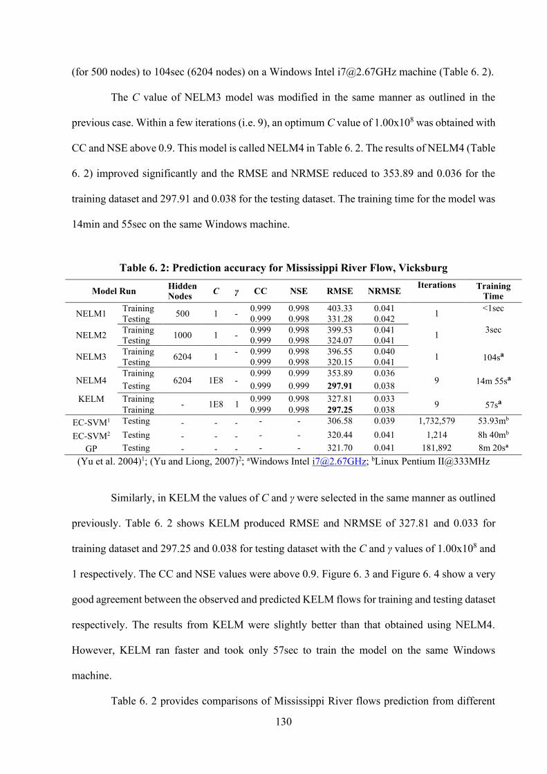
130

(for 500 nodes) to 104sec (6204 nodes) on a Windows Intel [email protected] machine (Table 6. 2).

The C value of NELM3 model was modified in the same manner as outlined in the

previous case. Within a few iterations (i.e. 9), an optimum C value of 1.00x108 was obtained with

CC and NSE above 0.9. This model is called NELM4 in Table 6. 2. The results of NELM4 (Table

6. 2) improved significantly and the RMSE and NRMSE reduced to 353.89 and 0.036 for the

training dataset and 297.91 and 0.038 for the testing dataset. The training time for the model was

14min and 55sec on the same Windows machine.

Table 6. 2: Prediction accuracy for Mississippi River Flow, Vicksburg

Model Run Hidden Nodes C γ CC NSE RMSE NRMSE

Iterations Training Time

NELM1 Training 500 1 - 0.999 0.998 403.33 0.041 1 <1sec Testing 0.999 0.998 331.28 0.042

NELM2 Training 1000 1 - 0.999 0.998 399.53 0.041 1 3sec Testing 0.999 0.998 324.07 0.041

NELM3 Training 6204 1 - 0.999 0.998 396.55 0.040 1 104sa Testing 0.999 0.998 320.15 0.041

NELM4 Training

6204 1E8 - 0.999 0.999 353.89 0.036

9 14m 55sa Testing 0.999 0.999 297.91 0.038 KELM

Training - 1E8 1 0.999 0.998 327.81 0.033 9 57sa Training 0.999 0.998 297.25 0.038

EC-SVM1 Testing - - - - - 306.58 0.039 1,732,579 53.93mb

EC-SVM2 Testing - - - - - 320.44 0.041 1,214 8h 40mb

GP Testing - - - - - 321.70 0.041 181,892 8m 20sa

(Yu et al. 2004)1; (Yu and Liong, 2007)2; aWindows Intel [email protected]; bLinux Pentium II@333MHz

Similarly, in KELM the values of C and γ were selected in the same manner as outlined

previously. Table 6. 2 shows KELM produced RMSE and NRMSE of 327.81 and 0.033 for

training dataset and 297.25 and 0.038 for testing dataset with the C and γ values of 1.00x108 and

1 respectively. The CC and NSE values were above 0.9. Figure 6. 3 and Figure 6. 4 show a very

good agreement between the observed and predicted KELM flows for training and testing dataset

respectively. The results from KELM were slightly better than that obtained using NELM4.

However, KELM ran faster and took only 57sec to train the model on the same Windows

machine.

Table 6. 2 provides comparisons of Mississippi River flows prediction from different


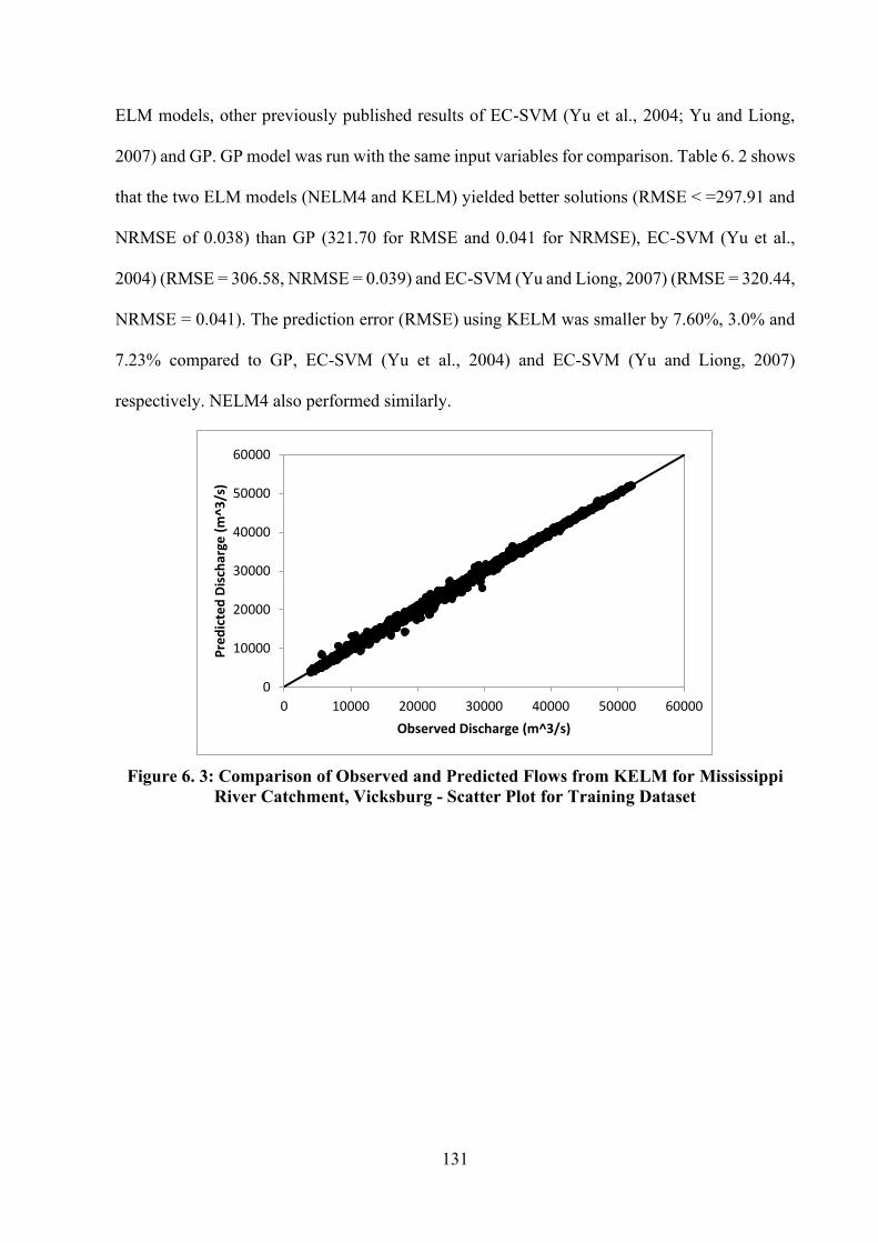
131

ELM models, other previously published results of EC-SVM (Yu et al., 2004; Yu and Liong,

2007) and GP. GP model was run with the same input variables for comparison. Table 6. 2 shows

that the two ELM models (NELM4 and KELM) yielded better solutions (RMSE < =297.91 and

NRMSE of 0.038) than GP (321.70 for RMSE and 0.041 for NRMSE), EC-SVM (Yu et al.,

2004) (RMSE = 306.58, NRMSE = 0.039) and EC-SVM (Yu and Liong, 2007) (RMSE = 320.44,

NRMSE = 0.041). The prediction error (RMSE) using KELM was smaller by 7.60%, 3.0% and

7.23% compared to GP, EC-SVM (Yu et al., 2004) and EC-SVM (Yu and Liong, 2007)

respectively. NELM4 also performed similarly.

Figure 6. 3: Comparison of Observed and Predicted Flows from KELM for Mississippi River Catchment, Vicksburg - Scatter Plot for Training Dataset

0

10000

20000

30000

40000

50000

60000

0 10000 20000 30000 40000 50000 60000

Pre

dic

ted

Dis

char

ge (

m^3

/s)


132

Figure 6. 4: Comparison of Observed and Predicted Flows from KELM for Mississippi River Catchment, Vicksburg - Scatter Plot for Testing Dataset

The time required by NELM4 and KELM to train input data were 14min 55sec and

57sec respectively from 9 iterations on a Windows Intel [email protected] machine. On the same

machine, GP took 8min 20 sec and 181,892 iterations to train the model. The number of iterations

and the training time required for EC-SVM (Yu et al., 2004) were 1,732,579 iterations and

53.93min respectively (see Table 4 in Yu et al., 2004) and for EC-SVM (Yu and Liong, 2007)

were 1,214 iterations and 8hr 40min (Table 6, Yu and Liong, 2007) respectively on a Linux

Pentium II@333mHz machine. KELM produced the best results converging very quickly in a

few iterations (< 10) to achieve the best results among the models compared.

6.6.3 Duckmaloi Catchment

ELM was applied to the Duckmaloi catchment with the lagged flow and rainfall data as

inputs (equation 1b). The number of hidden nodes in NELM1, NELM2 and NELM3 were 500,

1000 and 7745 respectively (refer to section 5.3.2 for details). These models used a C value of 1.

All three models ran fast and the maximum time required to train the model (NELM3) was

3.14min (Table 6. 3) on Windows Intel [email protected] machine. The models predict well and the

0

10000

20000

30000

40000

0 10000 20000 30000 40000

Pre

dic

ted

Dis

char

ge (

m^3

/s)




133

lowest RMSE and NRMSE for the testing dataset were obtained in the model with the highest

number of hidden nodes (7745 in NELM3). The CC and NSE values were above 0.9 and 0.8

respectively for all training and testing datasets. The RMSE ranged between 47.124-49.733 for

training and 33.099-41.165 for testing data (Table 6. 3). The corresponding NRMSE was between

0.382-0.404 for training and 0.284-0.353 for testing results.

Table 6. 3: Prediction Accuracy for Duckmaloi Weir Catchment

Model Run Hidden Nodes C γ CC NSE RMSE NRMSE

Iterations Training Time

NELM1 Training 500 1 - 0.915 0.837 49.733 0.404 1 1.31sec Testing 0.936 0.876 41.165 0.353

NELM2 Training 1000 1 - 0.919 0.844 48.659 0.395 1 3.95sec Testing 0.944 0.892 38.412 0.329

NELM3 Training 7745 1 - 0.924 0.854 47.124 0.382 1 3.14ma Testing 0.959 0.920 33.099 0.284

NELM4 Training

7745 10 - 0.929 0.862 45.766 0.371

2 6m 3sa Testing 0.962 0.923 32.487 0.278 KELM

Training - 1E3 10 0.929 0.862 45.748 0.371 5 1m 6sa Testing 0.961 0.923 32.404 0.278

GP Testing - - - - - 60.715 0.520 255,473 12.52ma

aWindows Intel [email protected]

The C value was then selected in a manner similar to previous cases and took two

iterations (see mode NELM4 in Table 6. 3) to improve the results with CC and NSE values above

0.9 and 0.8 respectively. The RMSE improved by 2.9% (from 47.124 to 45.766) for training

samples and 1.8% (from 33.099 to 32.487) for testing samples compared to NELM3 (see Table

6. 3). The NRMSE also reduced by 2.8% (from 0.382 to 0.371) for training dataset and 2.1%

(from 0.284 to 0.278) for testing dataset respectively. NELM4 took 6min 3sec to train the model.

The selection of parameters (C and γ) in KELM took five iterations to improve the

results with CC and NSE values above 0.9 and 0.8 respectively. The minimum RMSE values

obtained from this model were 45.748 and 32.404 and NRMSE were 0.371 and 0.278 for training

and testing datasets respectively (see Table 6. 3). Figure 6.5 and Figure 6.6 show the graphical

representation of scatter plot between the observed and predicted flows for training and testing

dataset. KELM required a short time (1min 6sec) to obtain this result.

134

Figure 6. 5: Comparison of Observed and Predicted Flows from KELM for Duckmaloi

Weir Catchment - Scatter Plot for Training Dataset

Figure 6. 6: Comparison of Observed and Predicted Flows from KELM for Duckmaloi

Weir Catchment - Scatter Plot for Testing Dataset

The performances of different ELM and GP models are compared in Table 6. 3. No

results were available for EC-SVM (Yu et al., 2004) or EC-SVM (Yu and Liong, 2007). ELM

models performed better than GP. Specifically, NELM4 and KELM reduced RMSE by more

than 46% compared to GP. GP required 255,473 iterations and 12.52mins to generate results with

a RMSE of 60.715 and NRMSE of 0.520. Both NELM4 and KELM produced similar results.

NELM4 ran slower than KELM as the run time of the former depended on the number of hidden

0

5

10

15

20

25

30

35

40

0 10 20 30 40

Pre

dic

ted

Dis

char

ge (

m^3

/s)


0

200

400

600

800

1000

1200

0 200 400 600 800 1000 1200

Pre

dic

ted

Dis

char

ge (

m^3

/s)


135

nodes in hidden layer.

6.7 Discussion

This chapter demonstrates the application of a fast AI technique called ELM.

Predictions of yields were undertaken for three catchments located in different continents each

with different climates namely the Tryggevælde catchment in Denmark, Mississippi River Flow

at Vicksburg in USA and Duckmaloi catchment in Australia. In the former two, lagged flows

were used as input consistent with other published techniques. In the later lagged flows and

rainfall were used as input. Performances of different types of ELMs (node based and kernel

based) were assessed in terms of CC, NSE, RMSE and NRMSE.

All NELM models generated good results (CC > 0.9 and NSE > 0.8). The best results

were obtained where the number of hidden nodes was set to the number of training samples in

node based ELM (NELM3). The performance was further improved by fine tuning the C

parameter in NELM4. It was found that within a few trials, the RMSE reduced to 0.486 (1.8%)

for Tryggevælde catchment, 297.91 (6.9%) for Mississippi River Catchment and 32.487 (1.8%)

for Duckmaloi catchment compared to NELM3. KELM produced similar or better results

compared to NELM4.

Both NELM4 and KELM produced better results compared to GP and EC-SVM when

predicting flow series for all three catchments. Compared to GP, KELM improved the prediction

accuracy by between 7.6-46.6% for these catchments. Similarly, KELM’s results were better

than that of EC-SVM (Yu and Liong, 2007) and showed improvement of 2.8% for Tryggevælde

catchment and 7.2% for Mississippi River catchment. KELM was also better than EC-SVM (Yu

et al., 2004). The performance of NELM4 was similarly better.

KELM was computationally much faster in training models than NELM, GP and EC-

SVM for all catchments noting that the computational time was not completely comparable since

136

two different types of machines were used. The performance of EC-SVM using Linux Pentium

II@333mHz machine was obtained from literature. ELM’s learning algorithm is much simpler,

and the learning speed is extremely fast as it avoids iterative tuning to determine the input weights

(Huang et al., 2006). KELM ran faster than NELM4 (Table 6. 1- Table 6. 3) as KELM does not

require information on the number of hidden nodes.

This analysis shows that even when using a simple parameter selection technique,

KELM produced results with better accuracy in much faster run time than any other model

studied here. Indeed, using a more sophisticated optimization techniques to select parameters C

and γ may further improve the performance of KELM (and NELM4) in terms of prediction

accuracy.

The major strength demonstrated in this analysis was KELM’s ability to reach similar

or better solutions much faster than NELM, GP and EC-SVM. It adds to its attractiveness for use

in actual river and flood operations and its potential for real-time prediction of hydrological time-

series and where quick model response is vital for decision making in application such as flood

warning and forecasting systems. It can make significant contribution in real-time control

applications.

6.8 Summary

The application of node and kernel based ELMs (NELM and KELM) were applied to

predict flows from three different catchments (Tryggevælde catchment, Denmark; Mississippi

River, USA and Duckmaloi catchment, Australia). The performances from different ELM

models were also compared with GP and EC-SVM. Predictions of daily flow time series from

all catchments showed how ELM could improve the prediction accuracies and reached the

optimal solutions faster than GP and EC-SVM. The study findings concluded that:

• KELM and NELM obtained good prediction accuracies for all catchments where CC

137

and NSE were greater than 0.9 and 0.8 respectively;

• NELM produced good results for all catchments where the number of hidden nodes was

greater than 1000. However, better results are obtained where the number of hidden

nodes was the same as the number of training samples. The time required to train the

model varied from less than a second to a few minutes.

• KELM produced similar or better results than NELM;

• Both NELM and KELM models were capable of producing better results compared to

GP and EC-SVM; and

• KELM computationally runs faster than NELM and other models as KELM does not

require hidden nodes.

This analysis shows that KELM produced more accurate results in much faster run

times than other models studied. The study demonstrates ELM’s ability, especially KELM’s,

for rapid prediction and has potential application in real-time river and flood forecasting and in

water resources planning and management.

138

CHAPTER 7

CONCLUSIONS AND RECOMMENDATIONS

139

7. Conclusions and Recommendations

7.1 Summary

Application of Artificial intelligence (AI) techniques to resolve complex nonlinear

hydrological flow prediction problem was demonstrated in this study as calibration of such

physical hydrological models using a trial and error method or optimization algorithm requires

considerable effort and experience particularly when the number of the calibration parameters is

large. AI based machine learning techniques have proven superior by the researchers in this

modeling process (e.g. flow prediction) compared to other conceptual and stochastic models

including Autoregressive (AR), Autoregressive Moving Average (ARMA), Autoregressive

Integrated Moving Average (ARIMA), Autoregressive moving average with Exogenous Inputs

(ARMAX) and Sacramento model. However, many of the AI based data-driven modelling

methods including traditional ANN learning algorithms are slow requiring numerous iterations

to generate optimal solutions and may not be suitable for real-time prediction where fast response

is desirable (e.g. flood control). In this study, GP was first applied to fill the data gaps and predict

long term flows from a dam catchment using a hybrid approach (linked with MIKE11-NAM).

While the application was successful and produced better results, it was found that GP suffered

from computational overhead in the learning process. A relatively new machine learning

technique, called Extreme Learning Machine (ELM) was proposed in this study. Three different

catchments from three different continents were considered.

Initially, AI model using GP was developed for the daily real-time flow prediction at

the Duckmaloi Weir catchment located in Oberon, Australia considering present and past

rainfalls and past measured flows. GP model showed better results than ANN and Sacramento

model. GP model is further improved by using hybrid method with MIKE11-NAM (refer to

Chapter 3). This approach is used when the measured or gauged flows are not complete or

missing and long-term inflow prediction is required for reservoir management. The future 100

140

year flows were predicted assuming two hypothetical rainfall time series. The results from this

hypothetical rainfall analysis show how the flow conditions vary in the dam catchment in drought

conditions. The analysis provides information about the potential application of the GP and

hybrid models in operation and management of water resources.

Chapter 4 presents the application of ELM for predicting hydrological flow time-series

for the Tryggevælde Catchment (Denmark) and Mississippi River at Vicksburg (USA). It is

demonstrated that ELM overcomes the slow learning issue and predicted hydrological time-

series very quickly. The results also show that the prediction accuracies of ELM are better than

ANN and other previously published techniques (e.g. EC-SVM, Standard Chaotic Approach and

Inverse Approach). The real strength of ELM is the short computational run-time to reach

solutions comparable with other techniques including EC-SVM. This is because ELM does not

require iteration whereas other techniques (e.g. EC-SVM) may require thousands of iterations

and much longer processing time to predict the same flow time-series and yet with less accuracy.

The robustness of ELM’s capability in predicting flows is described in Chapter 5 using

the same two catchments, e.g. Tryggevælde Catchment, Denmark and Mississippi River, USA

and also Duckmaloi Weir catchment, Australia. ELM’s performance is compared with EC-SVM

and GP especially for the first two catchment obtained from the literature. The results showed

how ELM improved prediction accuracies and reached the solutions very quickly compared to

GP and EC-SVM.

In addition to general node based ELM (NELM), the performance of a kernel based

ELM is reported in Chapter 6. The prediction accuracies from NELM and KELM are compared

for the two catchments as described above plus another catchment, Duckmaloi catchment from

Australia. The performances from different ELM models were also compared with GP and EC-

SVM. Predictions of daily flow time series from all three catchments showed how KELM could

improve the prediction accuracies and reached the optimal solutions faster than NELM, GP and

141

EC-SVM.

7.2 Conclusions

The conclusions of this study are described below:

Application of GP

• GP model showed better results than ANN and Sacramento model in the prediction of

daily flow from Duckmaloi Weir catchment located in Oberon, Australia.

• The hybrid model by linking GP model with MIKE11-NAM improved the results further.

This model is applicable when the measured or gauged flows are not complete or missing.

and long-term inflow prediction is required for reservoir management.

• The future 100 year flows were predicted assuming two hypothetical rainfall time series

using the hybrid model. These predicted flows can be used to manage extended drought

or flood conditions.

Application of ELM

• The application of ELM in the predictions of flows for Tryggevælde Catchment

(Denmark) and Mississippi River at Vicksburg (USA) showed better accuracies

compared to ANN and other previously published techniques (e.g. EC-SVM, Standard

Chaotic Approach and Inverse Approach).

• ELM predicted the same hydrological time-series faster than ANN and other previously

published techniques (e.g. EC-SVM, Standard Chaotic Approach and Inverse Approach).

Robustness of ELM

• ELM showed reasonable results with all combination of lagged input variables (two or

higher lagged variables) for 1-day lead prediction in terms of CC (>0.9) and NSE (>0.8).

For smaller catchment, higher number of lagged variables (2 or more for Tryggevælde

142

Catchment) produced better prediction as the catchment responds rapidly to change in

climatic condition (e.g. rainfall). However, a bigger catchment (e.g. Mississippi River)

responds slowly and higher number of lagged variables have minimal impact on the

prediction.

• ELM produced satisfactory results very rapidly when the number of hidden nodes was

greater than or equal to 1000. The computational time required by ELM ranges from less

than a second where the number of hidden nodes of the hidden layer were ten to two

minutes for maximum number of hidden nodes (number of training samples). The

number of hidden nodes higher than 1000 increased the computational run time

significantly (from less than a second to two minutes) with a minor improvement in

accuracy (<3%).

• ELM was able to extrapolate reasonably well where the input variables with highest flows

were excluded from training dataset.

• ELM showed improved results when the parameter of regularization coefficient was fine-

tuned.

• ELM generated reasonable results for higher number of lead days (e.g. second and third)

predictions.

• ELM produced similar or better results compared to GP and EC-SVM with a shorter

computational time for prediction of flow series from the same catchment.

Performance of Kernel ELM (KELM) compared to node ELM (NELM)

• KELM produced similar or more accurate results in much faster run times than NELM,

GP and EC-SVM. The study demonstrates ELM’s ability, especially KELM’s, for rapid

prediction and has potential application in real-time river and flood forecasting.

• ELM’s fast learning capability from a training dataset means that it would be more

suitable for on-line and real-time applications where quick processing is important or

143

vital. The study demonstrates ELM’s ability for rapid prediction and has potential

application in real-time forecasting and in water resources planning and management.

7.3 Limitations of the Study

Some of the limitations of the study are described below:

• Parameters including actual or potential evapotranspiration, antecedent

precipitation index, temperatures were not included in the input data.

• Important catchment characteristics including initial loss, continuous loss, area,

slope were not considered.

• The performances of the ELM model (NELM or KELM) were not tested for

real time prediction.

• ELM was not applied for different regional local catchments with different

climatic conditions.

7.4 Recommendations for Further Studies

The following recommendations are made for future extensions of this research work.

• Hydrological systems are generally complex and nonlinear. Time series of other

important and sensitive variables, e.g. total precipitation, antecedent

precipitation index, maximum temperature and evapotranspiration should be

considered if they are available. These additional inputs information may further

improve the prediction accuracies of the flows.

• This study has applied manual trial and error method to fine-tune some of the

parameters related to relevant AI techniques. Evolutionary algorithms including

both single-objectives and multi-objectives optimization are available. Single

objective algorithms, e.g. SCE, GA and PSO and multi-objective algorithm, e.g.

144

non-dominated sorting genetic algorithm (NSGA-II) should be linked with ELM

to automatically optimise the parameters such as regularisation coefficient (C)

and kernel parameter. Applying these automatic optimization algorithms may

improve the predictions significantly.

• ELM’s application was limited to three catchments obtained from the literature.

Further research will include ELM’s application to catchments from a wider

range of climatic condition and flow scenarios.

• ELM was applied to predict a single output. However, ELM’s performance in

predicting multiple outputs (objectives) should be investigated in the resolution

of complex problem.

145

REFERENCES

146

References

Adeli, A. and Sarma, K. C. (2006). “Cost Optimization of Structure – Fuzzy Logic, Genetic

Algorithms, and Parallel Computing”, John Wiley and Sons Australia Ltd, Australia.

Akhtar, M.K., Corzo, G.A., Andel, S.J., Jonoski, A. (2009). “River flow forecasting with

artificial neural networks using satellite observed precipitation pre-processed with flow

length and travel time information: case study of the Ganges river basin”, Hydrol. and

Earth Sys. Sci., 13, 1607-1618.

Al-Fayyaz, T. A. (2004). “Optimization of multi-objective reservoir operation system”, A Thesis

Submitted to NUS for the Degree of Master of Engineering, NUS, Singapore.

Alperovits, E. and Shamir, U. (1977). “Design of optimal water distribution systems.”, Water

Resources Research, Vol. 13(6), pp. 885-900.

Alvisi, S., Franchini, M. (2011). “Fuzzy neural networks for water level and discharge

forecasting with uncertainty”, Environ. Model. Softw. 26 (4), 523-537.

Alvisi, S., Franchini, M. (2012). “Grey neural networks for river stage forecasting with

uncertainty”, Phys. Chem. Of the Earth, 42-44, 108-118.

Amorocho, J. and Brandstetter. A. (1971). “Determination of Nonlinear Functional Response

Functions in Rainfall-Runoff Processes”, Water Resources Research, 7(5), pp.1087-1101.

Anctil, F., Michel, C., Perrin, C. and Andreassian, V. (2004). “A soil moisture index as an

auxiliary ANN input for stream flow forecasting”, Journal of Hydrology, 286, pp.155-167.

ASCE Task Committee (2000a). “Artificial Neural Networks in Hydrology-1: Preliminary

Concepts”, Journal of Hydrologic Engineering, ASCE, 5(2), pp.115-123.

ASCE Task Committee (2000b). “Artificial Neural Networks in Hydrology-2: Hydrologic

Applications”, Journal of Hydrologic Engineering, ASCE, 5(2), pp.124-137.

ASCE Task Committee (1993). “Definition of Criteria of Evaluation of Watershed Models”, J.

Irrigation and Drainage Engineering, 119 (3), pp.429-442.

147

Atiquzzaman, M. (2004). “Water distribution network modelling: Hydroinformatics Approach”,

A Thesis Submitted to NUS for the Degree of Master of Engineering, NUS, Singapore.

Atiquzzaman, M, Liong, S. Y. And Yu, X. (2006). “Alternative decision in water distribution

network with NSGA-II”. Journal of Water Resources Planning and Management, 132(2),

122-126.

Atiquzzaman, M., Kandasamy, J., (2016a). “Prediction of Inflows from Dam Catchment using

Genetic Programming”, Int. Journal of Hydrology Science and Technology, Vol. 6, No.

2, pp103-117.

Atiquzzaman, M., Kandasamy, J., (2016b). “Prediction of Hydrological Time-Series using

Extreme Learning Machine”, Journal of Hydroinformatics, 18.2, pp345-353.

Atiquzzaman, M., Liong, S.Y. (2004). “Using Shuffled Complex Evolution to Calibrate Water

Distribution Network Model.”, Journal of Civil Engineering, Institution of Engineers,

Bangladesh, Vol. 32, No.2, pp. 111-119.

Aytek, A. and Kisi, O. (2008). “A genetic programming approach to suspended sediment

modelling”, Journal of Hydrology, 351, 288-298.

Azamathulla, H. M., Ghani, A. A., Zakaria, N. A. and Guven, A. (2010). “Genetic Programming

to Predict Bridge Pier Scour”, Journal of Hydraulic Engineering, Vol. 136, No. 3, 165-

169.

Azamathulla, H. Md. and Zahiri, A. (2012) “Flow discharge prediction in compound channels

using linear genetic programming”, Journal of Hydrology, 454-455, pp.203-207.

Babovic, V. (1996). “Emergence, Evolution, Intelligence: Hydroinformatics”, Balkema

Publishers, Rotterdam.

Babovic, V. (1998). “A Data Mining Approach to Time Series Modeling and Forecasting”, In

Proc. of the 3rd. International Conference on Hydroinformatics '98, Balkema, Rotterdam,

pp.. 847-856.

148

Babovic, V. and Abbott, M. B. (1997) “The Evolution of Equations from Hydraulic Data, Part I:

Theory”, Journal of Hydraulic Research, IAHR 35(3), pp.397-410.

Babovic, V. and Keijzer, M. (2000) “Genetic Programming as a Model Induction Engine”,

Journal of Hydroinformatics, IWA 2(1), pp.35-60.

Babovic, V. and Keijzer, M. (2002) “Rainfall-runoff modelling based on Genetic Programming”,

Nordic Hydrology, 33(5), pp.331-346.

Babovic, V. and M.B. Abbott. (1997). “The Evolution of Equations from Hydraulic Data”, Part

II: Applications, Journal of Hydraulic Research, 35(3), pp. 411-430. 1997.

Babovic, V. (1996). “Emergence, Evolution, Intelligence; Hydroinformatics”, PhD Thesis.

Balkema Publishers. Rotterdam.

Babovic, V., Keijzer, M. & Bundzel, M. (2000), “From Global to Local Modelling: a Case Study

in Error Correction of Deterministic Models”, Hydroinformatics 2000, Iowa Institute of

Hydraulic Research, Iowa, USA.

Banihabib, M. E., Arabi, A. and Salha, A. A. (2015) “A dynamic artificial neural network for

assessment of land-use change impact on warning lead-time of flood”, International

Journal of Hydrology Science and Technology, 5(2), pp.163–178.

Boonya-Aroonnet, S. (2002). “Modelling of urban flooding in the Asian region”, Master Thesis

submitted to Asian Institute of Technology, Bangkok, Thailand.

Boucher, M.A., Perreault, L., Anctil, F. (2009). “Tools for the assessment of hydrological

ensemble forecasts obtained by neural networks”, J. Hydroinf. 11 (3), 297-306.

Burnash, R.J.C. (1995). “The NWS River Forecast System - Catchment Modeling”. In Computer

Models of Watershed Hydrology, ed by V. P. Singh, pp. 311-366. Colorado: Water

Resources Publications.

149

Cannas, B., Montisci, A., Fanni, A. (2004), “Comparing Artificial Neural Networks and Support

Vector Machines for Modelling Rainfall-Runoff”, Proceedings of the 6th of International

Conference on Hydroinformatics, Singapore.

Chen, Y., H and Chang, F., J, (2009). “Evolutionary Artificial Networks for Hydrological

Systems Forecasting”, Journal of Hydrology, 367, 125-137.

Chen, X.Y., Chau, K. W., Busari, A. O., (2015). “A comparative study of population-based

optimization algorithms for downstream river flow forecasting by a hybrid neural

network model,” Engineering Applications of Artificial Intelligence 46, pp. 258-268.

Cheng, C. T., Ou, C. P. and Chau, K. W. (2002). “Combining a fuzzy optimal model with a

genetic algorithm to solve multi-objective rainfall-runoff model calibration”, Journal of

Hydrology, 268, 72-86.

Chionga, G., Marcolini, G., Liu, W., Ciria, T. P. and Tuo, Y. (2018). “Coupling hydrological

modelling and support vector regression to model hydropeaking in alpine catchment”,

Science of The Total Environment, 633: 220-229.

Chiplunkar, A.V., Mehndiratta, S.L. and Khanna, P. (1986). “Looped water distribution system

optimization for single loading.”, Journal of Environmental Engineering.

Chiu, C.L. and J.T. Huang. (1970). “Non-Linear Time-Varying Model of Rainfall-Runoff

Relation”, Water Resources Research, 6(1), pp. 1277-1286.

Cieniawski, S. E., J. W. Eheart, and J. Ranjithan. (1995). “Using Genetic Algorithms to Solve

Groundwater Monitoring Problem”, Water Resources Research, 31(2), pp. 399-409.

Cigizoglu, H. K. (2003). “Estimation, forecasting and extrapolation of river flows by Artificial

Neural Networks”, Hydrological Science Journal, 48:3, 349-361.

Cui, L., Li, Y.P., Huang, G.H., Huang, Y. (2014). “Effects of digital elevation model resolution

on topography-based runoff simulation under uncertainty”, Journal of Hydroinformatics.

16(6), 1343-1358.

150

Cunha, M.D.C., and Sousa, J. (1999). “Water Distribution Network Design Optimization:

Simulated Annealing Approach.”, Journal of Water Resources Planning and

Management, Vol. 125, No. 4, pp. 215-221.

Dandy, G. C., A. R. Simpson, and L. J. Murphy. (1996). “An Improved Genetic Algorithm for

Pipe Network Optimization”, Water Resources Research, 32(2), pp. 449-458.

Deb, K., Agrawal, S., Pratap, A., and Meyarivan, T. (2000). “A fast elitist non-dominated sorting

genetic algorithm for multi-objective optimization: NSGA-II.” Proc., Parallel Problem

Solving from Nature VI Conf., Springer, France, 849–858.

Deka, P. C. and Chandramouli, V. (2009). “Fuzzy Neural Network modelling of reservoir

operation”, Journal of Water Resources Planning and Management, 135 (1), 5-12.

DHI (2013), MIKE 11 - NAM Technical Reference, Agern Alle 11, Horsholm, Denmark.

Dibike, Y. B. (2000), “Machine Learning Paradigms for Rainfall-Runoff Modelling”,

Hydroinformatics 2000, Iowa Institute of Hydraulic Research, Iowa, USA.

Ding, S., Zhao, H., Zhang, Y., Xu, X., Nie, R. (2015). “Extreme Learning Machine: Algorithm,

Theory and Application”, Artif. Intell. Rev, 44, 103-115.

DNR (2007) “Fish River Water Supply Scheme IQQM Modelling Report”, Report Prepared for

NSW Department of Natural Resources, March 2007.

Dorigo, M., Maniezzo, V., and Colorni, A. (1996). “The ant system optimization by a colony or

cooperating ants.”, IEEE Trans. Syst. Man. Cybern., 26, pp. 29-42.

Duan, N., Mays, L.W., and Lansey, K.E. (1990). “Optimal reliability-based design of pumping

and distribution systems.”, Journal of Hydraulic Engineering, ASCE, Vol. 116, No. 2, pp.

249-268.

Duan, Q., S. Sorooshian, and V. K. Gupta. (1992). “Effective and Efficient Global Optimization

for Conceptual Rainfall-Runoff Models”, Water Resources Research, 28(4), 1015-1031.

151

Duan, Q.Y., Gupta, V. K., and Sorooshian, S. (1993). “Shuffled Complex Evolution approach

for effective and efficient global minimization.”, Journal of Optimization Theory and

Applications, Vol. 76, No. 3, pp. 501-521.

Eiger, G., Shamir, U., and Ben-Tal A. (1994). “Optimal design of water distribution networks.”,

Water Resources Research, Vol. 30, No. 9, pp. 2637-2646.

Eusuff, M.M. and Lansey, K. E. (2003). “Optimization of Water Distribution Network Design

Using the Shuffled Frog Leaping Algorithm.”, Journal of Water Resources Planning and

Management, ASCE, Vol. 129, No. 3, pp. 210-225.

Fernando, D.A.K. and Jayawardena, A. W. (1998). “Runoff Forecasting using RBF networks

with OLS algorithm”, Journal of Hydrologic Engineering, 3(3), pp.203-209.

Fogel, L. J., A. J. Owens and M. J. Walsh. (1966). “Artificial Intelligence through Simulated

Evolution”, John Wiley, New York.

Fotovatikhah, F., Herrera, M., Shamshirband, S., Chau, K. W., Ardabili, F. S. and Piran, M. J.,

(2018). “Survey of Computational Intelligence as Basis to Big Flood Management:

Challenges, research directions and Future Work,” Engg. App. of Comput. Fluid Mech.,

12 (1), pp. 411-437.

Franchini, M., (1996). “Use of a Genetic Algorithm Combined with a Local Search Method for

the Automatic Calibration of Conceptual Rainfall-Runoff Models”, Journal of

Hydrological Sciences, Vol. 41(1), pp. 21-39.

Fujiwara, O., Jenchaimahakoon, B. and Edirisinghe, N. (1987). “A modified linear programming

gradient method for optimal design of looped water distribution networks.”, Water

Resources Research, Vol.-23, no. 6, pp. 977-982.

Fujiwara. O. and Khang, D. B. (1990). “A two-phase decomposition method for optimal design

of looped water distribution networks.”, Water Resources Research, Vol. 26, No. 4, pp.

539-549.

152

Funahashi K. (1989). “On the Approximate Realization of Continuous Mappings by Neural

Networks”, Neural Networks, 2, pp. 183-192.

Furundzic D. (1998) “Application Example of Neural Networks for Time Series

Analysis:Rainfall-RunoffModeling”, Signal Processing, 64, pp. 383-396.

Gallant, A.R. and H. White. (1992). “On Learning the Derivatives of an Unknown Mapping with

Multi-layer Feedforward Networks”, Neural Networks, 5, 129-138.

Gan, T. Y. and Biftu, G.F. (1996). “Automatic calibration of conceptual rainfall-runoff models:

Optimization algorithms, catchment conditions, and model structure”, Water Resources

Research, Vol. 32, No.12, pp. 3513-3524.

Gholami, V., Chau, K. W., Fadaie, F., Torkman, J. and Ghaffari, A. (2015). “Modelling of

groundwater level fluctuations using dendrochronology in alluvial aquifers”, Journal of

Hydrology, 529: 1060-1069.

Goldberg, D.E. (1989). “Genetic algorithms for search, optimization and machine leaning”,

Massachusetts: Addison-Wesley Publishing Co.

Gupta, I., Gupta, A., Khanna, P. (1999). “Genetic algorithm for optimization of water distribution

systems”, Environmental Modelling & software Vol.-4, pp. 437-446.

He, Z., Wen, X., Liu, H., Du, J., 2014. A comparative study of artificial neural network, adaptive

neuro fuzzy inference system and support vector machine for forecasting river flow in the

semiarid mountain region. Journal of Hydrology, 509, 379-386.

Holland, J. (1975). “Adaptation in natural and artificial systems.”, University of Michigan,

Illinois.

Hsu, K.L., Gupta, H.V. and Sorooshian, S. (1995). “Artificial Neural Network Modeling of the

Rainfall-Runoff Process”, Water Resources Research, 31(10), pp.2517-2530.

Huang G.-B., Wang, D. H. and Lan, Y. (2011). “Extreme Learning Machine: a Survey”,

International Journal of Machine Learning & Cybernetic, 2, pp 107-122.

153

Huang, G.B., Zhou, H., Ding, X., Zhang, R. (2012). “Extreme Learning Machine for Regression

and Multiclass Classification”, IEEE Tran.s on Sys., Man and Cyber-Part B: Cybernetics,

42(2), 513-529.

Huang, G.-B., Zhu Q.-Y., Siew C.-K. (2006). “Extreme Learning Machine: Theory and

Applications”, Neurocomput., 70, 489-501.

Huber, W. C., J. P. Heaney., S. J. Nix., R. E. Dickinson and D. J. Polman. (1988). “Storm Water

Management Model”, User's Manual, Version 4, EPA/600/3-88/001a (NTIS PB88-

236641/AS), U.S. Environmental Protection Agency, Athens, GA, 30605. 1988.

Ibrahim, Y. and S. Y. Liong, S.Y. (1992). “Calibration Strategy for Urban Catchment

Parameters”, Journal of Hydraulic Engineering, 118(10), pp. 1150-1570. 1992.

Jayawardena, A. W., Muttil, N and Fernando, T. M. K. G. (2005) “Rainfall-Runoff Modelling

using Genetic Programming. MODSIM05, International Congress on Modelling and

Simulation, Modelling and Simulation Society of Australia and New Zealand, December

2005, pp.1841-1847.

Jeevaragagam, P. and Simonovic, S. P. (2012) “Neural network approach to output updating for

the physically-based model of the Upper Thames River watershed”, International Journal

of Hydrology Science and Technology, 2(3), pp.306-324.

Johnston, P. R. and Pilgrim, D. H. (1976). “Parameter Optimization for Watershed Models,

Water Resources Research, 12(3), pp. 477-486.

Karunanithi, N., Grenney, W.J., Whitley, D. and K. Bovee (1994). Neural Networks for River

Flow Prediction. Journal of Computing in Civil Engineering, Vol. 8(2), pp.201-220.

Keijzer, M. and V. Babovic. (1999). “Dimensionally Aware Genetic Programming”, In Proc. of

the Genetic and Evolutionary Computation Conference (GECCO), Morgan Kaufmann,

CA., pp. 1065-1076.

154

Kennedy, J. and Eberhart, R.C. (1995). “Particle swarm optimization.”, Proc. of the IEEE Int.

Conf. on Neural Networks IV, Piscataway, NJ, pp. 1942-1948.

Kessler, A. and Shamir, U. (1989). “Analysis of the linear programming gradient method for

optimal design of water supply networks.”, Water Resources Research, Vol. 25, No.7, pp.

1469-1480.

Khu, S. T., Liong, S. Y., Babovic, V., Madsen, H. And Muttil, N. (2001), “Genetic Programming

and its Application in Real-Time Runoff Forecasting”, Journal of the American Water

Resources Association, Vol. 37, No. 2, pp. 439-451.

Kingston, G.B., Lambert, M.F., Maier, H.R. (2005). “Bayesian training of artificial neural

networks used for water resources modeling”, Water Resour. Res. 41(12) W12409.

Kirkpatrick, S., Gelatt, C., and Vecchi, M. (1983). “Optimization by simulated annealing.”, Sci.,

220 (4598), pp. 671-680.

Kisi, O., Shiri, J. and Tombul, M. (2013). “Modelling rainfall-runoff process using soft

computing techniques", Computer & Geosciences, 51, pp.108-117.

Koza, J. R. (1992). “Genetic Programming: On the Programming of Computers by Natural

Selection”, MIT Press, Cambridge, MA.

Koza, J. R. (1997). “Future Work and Practical Applications of Genetic Programming”, In

Handbook of Evolutionary Computation, ed by T. Baeck, D. B. Fogel and Z.

Michalewicz, Bristol, pp. H1.1:1-6. UK: Institute of Physics Publishing and New York:

Oxford University Press.

Krause, P., Boyle, D. P. And Base, F. (2005). “Comparison of different efficiency criteria for

hydrological model assessment”, Advances in Geosciences, 5, 89-97.

Kuczera, G. (1997). “Efficient Subspace Probabilistic Parameter Optimization for Catchment

Models”, Water Resources Research, 33(1), pp. 177-185.

155

Kulandaiswamy, V.C., and C.V. Subramanian. (1967). “A Non-linear Approach to Runoff

Studies”, In Proc of the International Hydrology Symposium, Fort Collins, Colorado, pp.

72-79.

Lall, H.S. and Percell, P.B. (1990). “A dynamic programming based gas pipeline optimizer,”,

Proceedings of the 9th international conference on analysis and optimization of systems,

Antibes, pp. 123-132.

Langdon, W.B. (1998). “Genetic Programming and Data Structure”. Kluwer Academic

Publishers, Norwell, Massachusetts.

Lansey, K. and Mays, L. (1989). “Optimal design of water distribution system design.”, Journal

of Hydraulic Engineering, Vol. 115, No. 10, pp. 1401-1418.

Lee, G. Y. and Suzuki, A. (1995) “Genetic Programming Approach for Time Series Analysis and

Prediction”, Journal of Graduate School and Faculty of Engineering, University of Tokyo

(B), 43(2), pp.201-220.

Li, B., Rong, X. and Li, Y. (2014). “An Improved Kernel Based Extreme Learning Machine for

Robot Execution Failures”, The Scientific World Journal, Hindawi Publishing

Corporation.

Lin, J.Y., Cheng, C.T., Chau, K.W. (2006). “Using Support Vector Machine for Long-Term

Discharge Prediction”, Hydrol. Sci., 51(4), 599-612.

Lin, S., Liu, X., Fang, J., Xu, Z., (2014). “Is Extreme Learning Machines Feasible? A Theoretical

Assessment (Part II).” Instit. for Informat. and Sys. Sci., School of Mathematics and

Statistics, Xi’an Jiaotong University, Xi’an 710049, China.

Liong, S. Y., Shree Ram, J. and Ibrahim, Y. (1995a). “Catchment Calibration Using Fractional-

Factorial and Central-Composite-Designs-based Response Surface”, Journal of

Hydraulic Engineering, 121(6), pp. 507-510.

156

Liong S.Y., Weng, T. C. and Shree Ram, J. (1995b). “Peak-flow Forecasting with Genetic

Algorithm and SWMM”, Journal of Hydraulic Engineering, 121(8), pp. 613-617.

Liong, S. Y. & Sivapragasam, C (2002). “Flood Stage Forecasting with SVM”, Journal of

American Water Reources Association, Vol. 38, Issue 1, pp. 173-186.

Liong, S. Y. And Atiquzzaman, M. (2004). “Optimal design of water distribution network using

Schuffled Complex Evolution”, Journal of the Institution of Engineers Singapore, 44(1),

93-107.

Liong, S. Y. and Y. Ibrahim. (1994). “Estimation of Peak Flow and Runoff Volume with

Response Surface Method”, Journal of Hydraulic Engineering, 120(2), pp. 161-175.

Liong, S. Y., Chan, W. T., and Lum, L. H. (1991). "Knowledge-based system for SWMM runoff

component calibration." ASCE Journal of Water Resources Planning and Management,

117(5), pp. 367-375.

Liong, S. Y., Gautam, T. R., Khu, S. T., Babovic, V., Muttil, N., (2002). “Genetic Programming:

A New Paradigm in Rainfall-Runoff Modelling”, Journal of American Water Resources

Association, 38(3): 705-718.

Liong, S. Y., Lim, W. H. and G.N. Paudyal. (1999). “River Stage Forecasting in Bangladesh:

Neural Network Approach”, Journal of Computing in Civil Engineering, ASCE. Vol.

14(1), pp.1-8.

Liong, S. Y., Phoon, K. K., Pasha, M. F. K. & Doan, C. D., 2002. “A robust and efficient scheme

in search for optimal prediction parameters set in chaotic time series”, First Asia Pacific

DHI Software Conference, Bangkok.

Liong, S.Y., S. T. Khu, and W. T. Chan. (2001). “Derivation of Pareto front With Genetic

Algorithms and Neural Networks”, Journal of Hydrologic Engineering 6 (1), pp. 52-61.

157

Lohani, A. K., Kumar R., Singh, R.D., (2012). “Hydrological Time Series: A Comparison

Between Adaptive Neuro-Fuzzy”, Neural Network and Autoregressive Techniques.

Journal of Hydrology 442-443, 23-35.

Madsen, H. (2000). “Automatic Calibration of a Conceptual Rainfall–Runoff Model using

Multiple Objectives, Journal of Hydrology, 235, pp. 276-288. 2000.

Maier, H.R., and Dandy, G.C. (2000). “Neural networks for prediction and forecasting of water

resources variables: a review of modelling issue and applications”, Environ. Model.

Softw. 15, 101-124.

Makkeasorn, A., Chang, N. B. and Zhou, X. (2008). “Short-term streamflow forecasting with

global climate change implications - A comparative study between genetic programming

and neural network models”, Journal of Hydrology, 352, pp.336-354.

Meshgi, A., Schmitter, P., Chui, T. F. M. and Babovic, V. (2015). “Development of a modular

streamflow model to quantify runoff contributions from different land uses in tropical

urban environments using Genetic Programming”, Journal of Hydrology, 525, 711-723.

Meteopolis, N., Rosenbluth, A., Rosenbluth, M., Teller, A., and Teller, E. (1953). "Equations of

state calculations by fast computing machines." Journal of Chemical Physics, 21, 1087-

1092.

Mittal, P, Chowdhury,S., Roy, S. Bhatia, N and Srivastav, R. (2012). "Dual Artificial Neural

Network for Rainfall-Runoff Forecasting," Journal of Water Resource and Protection,

Vol. 4 No. 12, pp. 1024-1028. doi: 10.4236/jwarp.2012.412118.

Morgan, D. and Goulter, I. (1985). “Water distribution design with multiple demands.”,

Proceedings of Specialty Conference on Computer Application in Water Resources,

ASCE, New York, pp. 582-590.

158

Mukerji, A., Chatterjee, C., Raghuwanshi, N. S., (2009). “Flood Forecasting Using ANN, Neuro-

Fuzzy and Neuro-GA Models”, Journal of Hydrologic Engineering Vol. 14, No. 6,

pp.647-652.

Nash, J. E. And Sutcliffe, J.V. (1970). “River Flow Forecasting through Conceptual Models,

Party I – A Discussion of Principles”, Journal of Hydrology, 10, 282-290.

Nelder, J.A. and Mead, R. (1965). “A simplex method for function minimization.”, Computer

Journal, Vol. 7, pp. 308-313.

Nielsen, S. A. and E. Hansen, E (1973). “Numerical Simulation of Rainfall-Runoff Process on a

Daily Basis”. Nordic Hydrology, 4, pp. 171-190.

Nourani, V Komasi, M. and Alami, T. (2013) “Geomorphology-based genetic programming

approach for rainfall-runoff modelling”, Journal of Hydroinformatics, 15(2), pp.427-445.

Ozelkan, E. C. and Duckstein, L. (2001), “Fuzzy Conceptual Rainfall-Runoff Models”, Journal

of Hydrology, 253, 41-68.

Perez, F.M.R. and Joaquin, I. (1995). “Optimum design and reliability in water distribution

systems.”, Proceeding of improving efficiency and reliability in water distribution

systems, pp. 303-328.

Peter, R. Schmitz, G. And Cullmann, J. (2006). “Flood Routing Modelling with Artificial Neural

Networks”, Advances in Geosciences, 9, 131-136.

Pham, D.T. and Karaboga, D. (2000). “Intelligent optimization techniques.”, Springer-Verlag,

London.

Phoon, K.K., Islam, M.N., Liaw, C.Y., Liong, S.Y. (2002) “Practical inverse approach for

forecasting nonlinear hydrological time-series”, J. Hydrol. Engng. 7(2), 116–128.

Poli, R., Langdon, W. B., McPhee, N. F. (2008). “A field guide to Genetic Programming”,

Creative Commons, San Francisco.

159

Quindry, G.E., Brill, E.D., and Liebman, J.C. (1981). “Optimization of looped water distribution

systems.”, Journal of Environmental Engineering Division, ASCE, Vol. 107, No. 4, pp.

665-679.

Rasouli, K., Hsieh, W. and Cannon, A. (2012). “Daily streamflow forecasting by machine

learning methods with weather and climate inputs”, Journal of Hydrology, 414-415, 284-

293.

Rathinasamy, M., Khosa, R., Adamowski, Ch, J. S., Partheepan, G., Anand, J. and Narsimlu, B.

(2014). “Wavelet-based multiscale performance analysis: An approach to assess and

improve hydrological models.” Water Resour. Res., 50, pp. 9721–9737.

Rodriguez-Vazquez, K. and P. J. Fleming. (1997). “A Genetic Programming/NARMAX

Approach to Non-linear System Identification”, Genetic algorithms in Engineering

systems: Innovations and applications.

Rodriguez-Vazquez, K., Arganis-Juarez, M.L., Cruickshank-Villanueva, C., Dominguez-Mora,

R. (2012). “Rainfall-Runoff Modelling using Genetic Programming”, J. of Hydroinf.,

14(1), 108-121.

Savic, D., Walters, G. A. and Davidson, J. W. (1999). “A Genetic Programming Approach to

Rainfall-Runoff Modelling”, Water Resources Management, 13, 219-231.

Savic, D.A. and Walters, G.A. (1997). “Genetic algorithms for least-cost design of water

distribution networks.”, Journal of Water Resources Planning and Management, ASCE,

Vol. 123, No. 2, pp. 67-77.

Schmidt, M., and Lipson, H. (2009) “Distilling Free-Form Natural Laws from Experimental

Data”, Science, 324(5923), pp. 81-85.

Schwefel, H-P. (1981). “Numerical Optimization of Computer Models”, Wiley, Chichester.

160

Simpson, A.R., Dandy, G.C., and Murphy, L.J. (1994). “Genetic algorithms compared to other

techniques for pipe optimization.”, Journal of Water Resources Planning and

Management, ASCE, Vol. 120, No. 4, pp. 423-443.

Sing, G., Panda, R.K., Lamers, M. (2015). “Modelling of Daily Runoff from a Small Agricultural

Watershed using Artificial Neural Network with Resampling Techniques”, J. of

Hydroinf., 17(1), 56-74.

Singh, V.P. (1988). “Hydrologic systems: rainfall-runoff modelling”, I, Prentice-Hall Press.

1988.

Singh, V.P. (1964). “Non-linear Instantaneous Unit Hydrograph Theory, Journal of the

Hydraulics Division”, Proceedings of ASCE, 90(HY2), pp. 313-347.

Sivapragasam, C. (2002). “Multi-Objective Evolutionary Techniques in Defining Optimal

Policies for Real Time Operation of reservoir Systems, PhD Thesis”, National University

of Singapore, Singapore.

Sivapragasam, C. and Liong, S. Y. (2002). “Flood Stage Forecasting with SVM”, Journal of

American Water Resources Association, 38(1), pp.173-186.

Sivapragasam, C. and Mutitil, N. (2005). “Discharge rating curve extension – a new approach”,

Water Resources Management, 19: 505-520.

Sivapragasam, C., and Liong, S. Y. (2000). “Improving Higher Lead Period Runoff Forecasting

Accuracy: The SVM Approach”, In Proc. of the 12th Congress of Asia and Pacific

Regional Division of IAHR, Vol. 3, Bangkok, pp. 855-862.

Sivapragasam, C., Liong S.Y. and Pasha, M. F. K. (2001). “Rainfall and Runoff Forecasting with

SSA-SVM Approach”, Journal of Hydroinformatics, 3(3), pp.141-152.

Sorooshian, S., Q. Duan, and V. K. Gupta. (1993). “Calibration of Rainfall-Runoff Models:

Application of Global Optimization to the Sacramento Soil Moisture Accounting Model”,

Water Resources Research, 29(4), pp. 1185-1194.

161

Su, Y.C., Mays, L.W., Duan, N., and Lansey, K. E. (1987). “Reliability-based optimization

model for water distribution systems.”, Journal of Hydraulic Engineering, ASCE, Vol.

114, No.12, pp. 1539-1556.

Sugawara, M. (1995). “Tank model, In Computer Models of Watershed Hydrology, ed by V. P.

Singh”, pp. 165-214. Water Resources Publications, Colorado.

Takahashi, Y. (1993). “Generalization and Approximation Capabilities of Multi-layer

Networks”, Neural Computation, 5, pp. 132-139.

Talei, A., Chua, L. H. C., (2012). “Influence of lag time on event-based rainfall-runoff modeling

using the data driven approach”. Journal of Hydrology, 438-439, pp.223-233.

Taormina, R. and Chau, K. W., (2015). “Data-driven input variable selection for rainfall-runoff

modelling using binary-coded particle swarm optimization and Extreme Learning

Machines”, Journal of Hydrology, 529 (3): pp. 1617-1632.

Tayfur, G. and Sing, V. P. (2006) “ANN and Fuzzy Logic Models for Simulating Event-Based

Rainfall-Runoff”, Journal of Hydraulic Engineering, 132(12), pp.1321-1330.

Thyer, M., Kuczera, G. and Bates, B.C. (1999). “Probabilistic optimization for conceptual

rainfall-runoff models: A comparison of the shuffled complex evolution and simulated

annealing algorithms.”, Water Resources Research, Vol. 35, No. 3, pp. 767-773.

Tingsanchali, T. and Quang C. N. X. (2004). “Application of Neuro-Fuzzy Technique in Flood

Forecasting”, 6th International Conference on Hydroinformatics, Singapore.

Todini, E. (1996). “The ARNO Rainfall-Runoff Model: Past Present and Future”, Journal of

Hydrology. 100, pp. 341-352.

Tokar, A.S., Johnson, P.A. (1999). “Rainfall-runoff modelling using Artificial Neural Network”,

J. of Hydrol. Engng, 4(3), 232-239.

162

Toth, E., A. Montanari and A. Brath. (1999). “Real time Flood Forecasting via Combined use of

Conceptual and Stochastic Models”, Physics and Chemistry of the Earth, Part B:

Hydrology, Oceans and Atmosphere, 24(7), pp. 793-798.

Tu, M-Y., Hsu, N-S. and Yeh, W. W-G., (2003). “Optimization of Reservoir Management and

Operation with Hedging Rules”, Journal of Water Resources Planning and Management,

Vol. 129, No. 2, pp. 86-97.

Vamvakeridou-Lyroudia, L.S. (1993). “Distribution network optimization using dynamic

programming.”, In: Water Supply Systems: State of the Art and Future Trends, Edited by

E. Cabrera and F. Martinez, Computational Mechanics, Southampton, UK.

Vapnik, V. (1999). “An Overview of Statistical Learning Theory”, IEEE Transactions on Neural

Networks. Vol. 10(5), pp.988-999.

Vemuri, V.R. and R.D. Rogers (ed) (1994). “Artificial Neural Networks: Forecasting Time

Series”, California: IEEE Computer Society Press.

Wang, Q.J., Chiew, F. H. S. and T. A. McMahon, T.A. (1995). “Calibration of environmental

models by genetic algorithms, paper presented at MODIM 1995: International Congress

on Modelling and Simulation”, Modelling and Simulation Society of Australia,

Newcastle.

Wang, Q. J., (1991). “The Genetic Algorithm and Its Application to Calibrating Conceptual

Rainfall-Runoff Models”, Journal of Water Resources Research, Vol. 27(9), pp. 2467-

2471.

Wang, X., Be, L. Li., Lockington, D., Pullar, D. and Jeng, D-S. (2005). “Self-Organizing

Polynomial Neural Network for modelling complex hydrological process”, Research

Report No R861, Department of Civil Engineering and Environmental Fluids/Wind

Group, The University of Sydney.

163

Wang, W-C., Chau, K-W., Cheng, C-T. and Qiu, L. (2009). “A Comparison of performance of

several artificial intelligence methods for forecasting monthly discharge time series”,

Journal of Hydrology, 374, 294-306.

Wang, W-C., Xu, D-M, Chau, K-W., Chen, S. (2013). “Improved Annual Rainfall-Runoff

Forecasting using PSO-SVM Model based on EEMD”, J. of Hydroinf., 15(4), 1377-1390.

Whigham, P. A. and Crapper, P. E. (2001). “Modelling Rainfall-Runoff Relationships using

Genetic Programming”, Mathematical and Computer Modelling, 33, pp.707-721.

Wong, P.J. and Larson, R.E. (1968). “Optimization of natural gas pipeline systems via dynamic

programming.”, IEEE Trans. Auto. Control, AC-13(5), pp. 475-481.

Wu, C. L. and Chau, K-W. (2011). “Rainfall-runoff modelling using Artificial Neural Network

coupled with Singular Spectrum Analysis”, Journal of Hydrology, 399 (3-4), 394-409.

Young, P. and S. Wallis. (1985). “Recursive Estimation: A Unified Approach to the

Identification, Estimation, and Forecasting of Hydrological Systems”, Applied

Mathematics and Computation, 17, pp. 299-334.

Yu, X. Y., Liong, S. Y., and Babovic, V. (2002). “An Approach Combining Chaos Theoretic

Approach and Support Vector Machine: Case Study in Hydrologic Forecasting”, In

Proceedings of 13th APD-IAHR Congress, Singapore, pp.690-695.

Yu, X., and Liong, S. Y., (2007). Forecasting of hydrological time series with ridge regression

in feature space. Journal of Hydrology 332 (3-4), 290-302.

Yu, X., Liong, S.Y., and Babovic, V. (2004). “EC-SVM approach for real-time hydrologic

forecasting”, J. of Hydroinf., 06(3), 209-223.

Yu, X., Y. and Liong, S. Y. (2004). “Enhanced Support Vector Machine for hydrological time

series forecasting”, 14th APD-IAHR Congress, Hong Kong.

Zadeh, L. A. (1965), “Fuzzy Set”, Information and Control, 8, 338-353.

164

Zhang, R., Huang, G-B., Sundararajan, N., Saratchandran, P. (2007). “Multi-category

Classification Using and Extreme Learning Machine for Microarray Gene Expression

Cancer Diagnosis”, IEEE/ACM Transac. on Comput. Biol. and Bioinf., 4(3), 485-495.

Documents

Improving Reliability of Hydrological Flow Estimation