Embed Size (px)
Citation preview

Improving Large-Scale Network Traffic Simulation
with Multi-Resolution Models
Dartmouth Computer Science Technical Report TR2005-558
A Thesis
Submitted to the Faculty
in partial fulfillment of the requirements for the
degree of
Doctor of Philosophy
in
Computer Science
by
Guanhua Yan
DARTMOUTH COLLEGE
Hanover, New Hampshire
September, 2005
Examining Committee:
(chair) David Kotz
Sean W. Smith
M. Douglas McIlroy
David M. Nicol (UIUC)
Charles K. Barlowe, Ph.D.Dean of Graduate Studies

Abstract
Improving Large-Scale Network Traffic Simulation
with Multi-Resolution Models
Dartmouth Computer Science Technical Report TR2005-558by
Guanhua YanDoctor of Philosophy in Computer Science
Dartmouth College, Hanover, NHSeptember 2005
Simulating a large-scale network like the Internet is a challenging undertaking because of thesheer volume of its traffic. Packet-oriented representation provides high-fidelity details but is com-putationally expensive; fluid-oriented representation offers high simulation efficiency at the priceof losing packet-level details. Multi-resolution modeling techniques exploit the advantages of bothrepresentations by integrating them in the same simulation framework. This dissertation presentssolutions to the problems regarding the efficiency, accuracy, and scalability of the traffic simula-tion models in this framework. The “ripple effect” is a well-known problem inherent in event-driven fluid-oriented traffic simulation, causing explosion of fluid rate changes. Integrating multi-resolution traffic representations requires estimating arrival rates of packet-oriented traffic, calculat-ing the queueing delay upon a packet arrival, and computing packet loss rate under buffer overflow.Real time simulation of a large or ultra-large network demands efficient background traffic simu-lation. The dissertation includes a rate smoothing technique that provably mitigates the “ripple ef-fect”, an accurate and efficient approach that integrates traffic models at multiple abstraction levels,a sequential algorithm that achieves real time simulation of the coarse-grained traffic in a networkwith 3 tier-1 ISP (Internet Service Provider) backbones using an ordinary PC, and a highly scalableparallel algorithm that simulates network traffic at coarse time scales.
ii

Acknowledgments
I want to give my utmost gratitude to Professor David Nicol, my research advisor, for his supportand guidance on my thesis research. His broad knowledge assisted me through my graduate studies;his sharp insight helped me identify interesting research problems; his high standard was the drivingforce behind my thesis work. I look forward to collaborating with him in the future.
I would also like to thank my dissertation committee, Professor David Kotz, Professor SeanSmith, and Professor Doug McIlroy for many helpful suggestions and advice. Some of their com-ments on my thesis will motivate me for further exploration in the field of network simulation.
This dissertation was made possible only after many inspiring discussions with my colleagues,especially Michael Liljenstam, Jason Liu, Yougu Yuan, and Meiyuan Zhao. I thank Felipe Per-rone for offering me to use his multiprocessor. I also want to express my gratitude to the peoplein the Computer Science Department at Dartmouth College, the staff in the Institute of SecurityTechnology Studies, and the staff in the Coordinated Science Laboratory at University of Illinois,Urbana-Champaign. They offered me tremendous help throughout my graduate studies.
I want to thank all the friends with whom I spent my time in the last five years. They includeCaie Yan, Dongsheng Zhang, Yaozhong Zou, Qing Feng, Shengyi Ye, Cheng Zhong, Feng Cao,Puxuan Dong, Yijin He, Xiang Li, Zhan Xiao, Qun Li, Guofei Jiang, and many many others.
I would like to express my greatest gratitude to my parents and my brothers for their love andsupport. Their encouragement has been a great source of inspiration in my life.
Funding
This research was supported in part by DARPA Contract N66001-96-C-8530, and NSF Grant CCR-0209144. Accordingly, the U.S. Government retains a non-exclusive, royalty-free license to publishor reproduce the published form of this contribution, or allow others to do so, for U.S. Governmentpurposes. In addition this research program is also a part of the Institute for Security TechnologyStudies, supported under Award number 2000-DT-CX-K001 from the Office for Domestic Prepared-ness, U.S. Department of Homeland Security, Science and Technology Directorate. Points of viewin this document are those of the author and do not necessarily represent the official position of theU.S. Department of Homeland Security or the Science and Technology Directorate.
iii

Contents
1 Introduction 1
1.1 Motivations . . . . . . . . . . . . . . . . . . . . . . . . . . . . . . . . . . . . . . 3
1.1.1 Limitations of Alternative Solutions . . . . . . . . . . . . . . . . . . . . . 3
1.1.2 Advantages of Simulation . . . . . . . . . . . . . . . . . . . . . . . . . . 4
1.1.3 Challenges in Large-Scale Network Simulations . . . . . . . . . . . . . . 5
1.2 Research Objectives and Contributions . . . . . . . . . . . . . . . . . . . . . . . . 6
1.3 Thesis Organization . . . . . . . . . . . . . . . . . . . . . . . . . . . . . . . . . . 8
2 Background 9
2.1 Simulation . . . . . . . . . . . . . . . . . . . . . . . . . . . . . . . . . . . . . . . 9
2.1.1 Definitions, Motivations and Procedures . . . . . . . . . . . . . . . . . . . 9
2.1.2 Classifications of Simulation Models . . . . . . . . . . . . . . . . . . . . 12
2.2 Model Simplification . . . . . . . . . . . . . . . . . . . . . . . . . . . . . . . . . 13
2.2.1 General Techniques . . . . . . . . . . . . . . . . . . . . . . . . . . . . . . 13
2.2.2 Simplification of Traffic Models in Network Simulation . . . . . . . . . . 15
2.2.3 Simplification of Routing Protocols in Network Simulation . . . . . . . . . 18
2.3 Simulation Event Management . . . . . . . . . . . . . . . . . . . . . . . . . . . . 19
2.3.1 Simulation Event Set Algorithms . . . . . . . . . . . . . . . . . . . . . . 20
2.3.2 An Optimization for Network Simulation . . . . . . . . . . . . . . . . . . 21
2.4 Parallel and Distributed Simulation . . . . . . . . . . . . . . . . . . . . . . . . . . 21
2.4.1 General Techniques . . . . . . . . . . . . . . . . . . . . . . . . . . . . . . 22
2.4.1.1 Conservative Synchronization . . . . . . . . . . . . . . . . . . . 23
2.4.1.2 Optimistic Synchronization . . . . . . . . . . . . . . . . . . . . 24
2.4.2 Parallel and Distributed Network Simulation . . . . . . . . . . . . . . . . 25
2.5 Computation Sharing . . . . . . . . . . . . . . . . . . . . . . . . . . . . . . . . . 26
iv

2.6 Variance Reduction . . . . . . . . . . . . . . . . . . . . . . . . . . . . . . . . . . 27
2.7 Summary . . . . . . . . . . . . . . . . . . . . . . . . . . . . . . . . . . . . . . . 30
3 Multi-Resolution Traffic Simulation Framework 31
3.1 Multi-Resolution Traffic Simulation Framework . . . . . . . . . . . . . . . . . . . 31
3.2 Implementation in iSSFNet . . . . . . . . . . . . . . . . . . . . . . . . . . . . . . 34
3.3 Summary . . . . . . . . . . . . . . . . . . . . . . . . . . . . . . . . . . . . . . . 36
4 Event-Driven Fluid-Oriented Traffic Simulation 37
4.1 Background . . . . . . . . . . . . . . . . . . . . . . . . . . . . . . . . . . . . . . 38
4.2 Fluid Multiplexer . . . . . . . . . . . . . . . . . . . . . . . . . . . . . . . . . . . 40
4.2.1 A Discrete Event Fluid FIFO Port . . . . . . . . . . . . . . . . . . . . . . 41
4.2.2 Ripple Effect . . . . . . . . . . . . . . . . . . . . . . . . . . . . . . . . . 46
4.2.3 Rate Smoothing . . . . . . . . . . . . . . . . . . . . . . . . . . . . . . . . 48
4.3 Integration with Packet-Oriented Flows . . . . . . . . . . . . . . . . . . . . . . . 57
4.3.1 Effect of Packet Flows on Fluid Flows . . . . . . . . . . . . . . . . . . . . 57
4.3.2 Effect of Fluid Flows on Packet Flows . . . . . . . . . . . . . . . . . . . . 58
4.3.3 Simulation Results . . . . . . . . . . . . . . . . . . . . . . . . . . . . . . 61
4.3.3.1 Experiment 1: Dumbbell Topology with MMFM Traffic . . . . . 62
4.3.3.2 Experiment 2: ATT Backbone with MMFM Traffic . . . . . . . 70
4.4 Hybrid Simulation of TCP Traffic . . . . . . . . . . . . . . . . . . . . . . . . . . 74
4.4.1 Nicol’s Fluid Modeling of TCP . . . . . . . . . . . . . . . . . . . . . . . 74
4.4.1.1 Sending Rates . . . . . . . . . . . . . . . . . . . . . . . . . . . 75
4.4.1.2 Timers . . . . . . . . . . . . . . . . . . . . . . . . . . . . . . . 76
4.4.1.3 Loss Recovery . . . . . . . . . . . . . . . . . . . . . . . . . . . 77
4.4.2 Modifications . . . . . . . . . . . . . . . . . . . . . . . . . . . . . . . . . 77
4.4.3 Simulation Results . . . . . . . . . . . . . . . . . . . . . . . . . . . . . . 80
4.4.3.1 Accuracy . . . . . . . . . . . . . . . . . . . . . . . . . . . . . . 81
4.4.3.2 Execution Speedup . . . . . . . . . . . . . . . . . . . . . . . . 83
4.5 Related Work . . . . . . . . . . . . . . . . . . . . . . . . . . . . . . . . . . . . . 87
4.6 Summary . . . . . . . . . . . . . . . . . . . . . . . . . . . . . . . . . . . . . . . 88
5 Time-Stepped Coarse-Grained Traffic Simulation 90
5.1 Background . . . . . . . . . . . . . . . . . . . . . . . . . . . . . . . . . . . . . . 91
5.2 Solution Outline . . . . . . . . . . . . . . . . . . . . . . . . . . . . . . . . . . . . 91
v

5.3 Problem Formulation . . . . . . . . . . . . . . . . . . . . . . . . . . . . . . . . . 93
5.4 Solutions in Specific Settings . . . . . . . . . . . . . . . . . . . . . . . . . . . . . 95
5.4.1 Networks with Sufficient Bandwidth . . . . . . . . . . . . . . . . . . . . . 95
5.4.2 Feed-Forward Networks with Limited Bandwidth . . . . . . . . . . . . . . 95
5.4.3 Networks with Circular Dependencies . . . . . . . . . . . . . . . . . . . . 96
5.5 Sequential Algorithm . . . . . . . . . . . . . . . . . . . . . . . . . . . . . . . . . 102
5.5.1 Algorithm Description . . . . . . . . . . . . . . . . . . . . . . . . . . . . 102
5.5.2 Convergence Behavior . . . . . . . . . . . . . . . . . . . . . . . . . . . . 116
5.5.3 Performance . . . . . . . . . . . . . . . . . . . . . . . . . . . . . . . . . 125
5.5.4 Accuracy . . . . . . . . . . . . . . . . . . . . . . . . . . . . . . . . . . . 127
5.6 Flow Merging . . . . . . . . . . . . . . . . . . . . . . . . . . . . . . . . . . . . . 130
5.7 Parallel Algorithm . . . . . . . . . . . . . . . . . . . . . . . . . . . . . . . . . . 133
5.7.1 Algorithm Description . . . . . . . . . . . . . . . . . . . . . . . . . . . . 135
5.7.2 Scalability Analysis . . . . . . . . . . . . . . . . . . . . . . . . . . . . . 141
5.7.2.1 Scalability with Fixed Problem Size . . . . . . . . . . . . . . . 141
5.7.2.2 Scalability with Scaled Problem Size . . . . . . . . . . . . . . . 145
5.8 Rule Modifications for Multi-Class Networks . . . . . . . . . . . . . . . . . . . . 151
5.9 Related Work . . . . . . . . . . . . . . . . . . . . . . . . . . . . . . . . . . . . . 154
5.10 Summary . . . . . . . . . . . . . . . . . . . . . . . . . . . . . . . . . . . . . . . 156
6 Conclusions and Future Work 157
6.1 Contributions . . . . . . . . . . . . . . . . . . . . . . . . . . . . . . . . . . . . . 157
6.2 Limitations . . . . . . . . . . . . . . . . . . . . . . . . . . . . . . . . . . . . . . 158
6.3 Future Work . . . . . . . . . . . . . . . . . . . . . . . . . . . . . . . . . . . . . . 159
6.3.1 Simulation-Based Online Network Control . . . . . . . . . . . . . . . . . 159
6.3.2 Load Balancing in High-Fidelity Network Simulation . . . . . . . . . . . . 160
6.3.3 Large-Scale Distributed Application Traffic Simulation . . . . . . . . . . . 160
6.3.4 Multi-Resolution Wireless Network Simulation . . . . . . . . . . . . . . . 160
6.4 Final Remarks . . . . . . . . . . . . . . . . . . . . . . . . . . . . . . . . . . . . . 161
vi

List of Tables
2.1 Analytical Performance of Event Set Algorithms . . . . . . . . . . . . . . . . . . 20
4.1 Notations . . . . . . . . . . . . . . . . . . . . . . . . . . . . . . . . . . . . . . . 41
4.2 Formalization of Cases 1 and 2 . . . . . . . . . . . . . . . . . . . . . . . . . . . . 42
4.3 Formalization of Cases 3 and 4 . . . . . . . . . . . . . . . . . . . . . . . . . . . . 43
4.4 Average Execution Time for Simulating ATT Topology . . . . . . . . . . . . . . . 72
5.1 Rule 1 . . . . . . . . . . . . . . . . . . . . . . . . . . . . . . . . . . . . . . . . . 104
5.2 Rule 2 . . . . . . . . . . . . . . . . . . . . . . . . . . . . . . . . . . . . . . . . . 104
5.3 Rule 3 . . . . . . . . . . . . . . . . . . . . . . . . . . . . . . . . . . . . . . . . . 106
5.4 Rule 4 . . . . . . . . . . . . . . . . . . . . . . . . . . . . . . . . . . . . . . . . . 106
5.5 Rule 5 . . . . . . . . . . . . . . . . . . . . . . . . . . . . . . . . . . . . . . . . . 107
5.6 Rule 6 . . . . . . . . . . . . . . . . . . . . . . . . . . . . . . . . . . . . . . . . . 108
5.7 Two Configurations . . . . . . . . . . . . . . . . . . . . . . . . . . . . . . . . . . 111
5.8 Flow Update Computation for the Network in Figure 5.5 (Configuration 1) . . . . . 112
5.9 Flow Update Computation for the Network in Figure 5.5 (Configuration 2) . . . . . 113
5.10 4 Topologies Used in the Simulations . . . . . . . . . . . . . . . . . . . . . . . . 118
5.11 Average Execution Time per Time-Step . . . . . . . . . . . . . . . . . . . . . . . 127
5.12 Average Execution Time per Time-Step Using Flow Merging Technique . . . . . . 132
5.13 Proportion of Execution Time Consumed by Each Phase w.r.t the Average ExecutionTime per Time Step . . . . . . . . . . . . . . . . . . . . . . . . . . . . . . . . . . 145
5.14 Implementation of GPS Scheduling Policy . . . . . . . . . . . . . . . . . . . . . . 152
5.15 Rule 2’ . . . . . . . . . . . . . . . . . . . . . . . . . . . . . . . . . . . . . . . . 153
vii

List of Figures
2.1 The Life Cycle of A Simulation Study . . . . . . . . . . . . . . . . . . . . . . . . 11
2.2 State Aggregation in Space Domain . . . . . . . . . . . . . . . . . . . . . . . . . 14
2.3 State Aggregation in Time Domain . . . . . . . . . . . . . . . . . . . . . . . . . . 15
2.4 Event-Driven Fluid-Oriented Traffic Model from an On/Off Source . . . . . . . . . 17
2.5 Illustration of Time-Driven Fluid-Oriented Simulation . . . . . . . . . . . . . . . 18
2.6 Packet Events on A High Bandwidth-Delay Product . . . . . . . . . . . . . . . . . 21
2.7 Logical Process Simulation . . . . . . . . . . . . . . . . . . . . . . . . . . . . . . 23
3.1 Multi-Resolution Traffic Simulation Framework . . . . . . . . . . . . . . . . . . . 32
3.2 An Example Topology with Multi-Resolution Traffic Representations . . . . . . . 33
3.3 Implementation in iSSFnet . . . . . . . . . . . . . . . . . . . . . . . . . . . . . . 35
4.1 Illustration of MMFM Traffic Model . . . . . . . . . . . . . . . . . . . . . . . . . 38
4.2 Slow Start Phase in A Fluid-Based TCP Model . . . . . . . . . . . . . . . . . . . 39
4.3 Illustration of A Discrete Event Fluid FIFO Port . . . . . . . . . . . . . . . . . . . 45
4.4 A Feed-Forward Topology . . . . . . . . . . . . . . . . . . . . . . . . . . . . . . 47
4.5 Rate Smoothing . . . . . . . . . . . . . . . . . . . . . . . . . . . . . . . . . . . . 48
4.6 Rate Change Matrix . . . . . . . . . . . . . . . . . . . . . . . . . . . . . . . . . . 49
4.7 The POP-Level ATT Backbone . . . . . . . . . . . . . . . . . . . . . . . . . . . . 51
4.8 Results on Unconstrained Rate Smoothing . . . . . . . . . . . . . . . . . . . . . . 55
4.9 Results on Constrained Rate Smoothing . . . . . . . . . . . . . . . . . . . . . . . 56
4.10 Integration of Packet And Fluid Flows . . . . . . . . . . . . . . . . . . . . . . . . 57
4.11 Dumbbell Topology . . . . . . . . . . . . . . . . . . . . . . . . . . . . . . . . . . 62
4.12 Packet Loss Probability under 10 Background Flows . . . . . . . . . . . . . . . . 63
4.13 TCP Goodput under 10 Background Flows . . . . . . . . . . . . . . . . . . . . . . 64
4.14 TCP Round Trip Time under 10 Background Flows . . . . . . . . . . . . . . . . . 65
viii

4.15 Delivered Fraction of UDP Traffic under 10 Background Flows . . . . . . . . . . . 65
4.16 Packet Loss Probability under 100 Background Flows . . . . . . . . . . . . . . . . 66
4.17 TCP Goodput under 100 Background Flows . . . . . . . . . . . . . . . . . . . . . 67
4.18 TCP Round Trip Time under 100 Background Flows . . . . . . . . . . . . . . . . 68
4.19 Delivered Fraction of UDP Traffic under 100 Background Flows . . . . . . . . . . 69
4.20 Speedup of Hybrid Simulation over Pure Packet-Level Simulation under DumbbellTopology . . . . . . . . . . . . . . . . . . . . . . . . . . . . . . . . . . . . . . . 70
4.21 TCP Goodput under ATT Topology . . . . . . . . . . . . . . . . . . . . . . . . . 72
4.22 Delivered Fraction of UDP Traffic under ATT Topology . . . . . . . . . . . . . . . 73
4.23 Speedup of Hybrid Simulation over Pure Packet-Level Simulation under ATT Topol-ogy . . . . . . . . . . . . . . . . . . . . . . . . . . . . . . . . . . . . . . . . . . 73
4.24 Packet Loss Probability under 10 TCP Flows . . . . . . . . . . . . . . . . . . . . 81
4.25 TCP Goodput under 10 TCP Flows . . . . . . . . . . . . . . . . . . . . . . . . . . 82
4.26 TCP Round Trip Time under 10 TCP Flows . . . . . . . . . . . . . . . . . . . . . 83
4.27 Packet Loss Probability under 100 TCP Flows . . . . . . . . . . . . . . . . . . . . 84
4.28 TCP Goodput under 100 TCP Flows . . . . . . . . . . . . . . . . . . . . . . . . . 85
4.29 TCP Round Trip Time under 100 TCP Flows . . . . . . . . . . . . . . . . . . . . 86
4.30 Execution Speedup of Hybrid Simulation over Pure Packet-Level Simulation . . . 86
5.1 Relationship between Foreground Traffic Simulation and Background Traffic Com-putation . . . . . . . . . . . . . . . . . . . . . . . . . . . . . . . . . . . . . . . . 93
5.2 A Five-Port Ring Topology . . . . . . . . . . . . . . . . . . . . . . . . . . . . . . 97
5.3 The Condensed Graph of The Feed-Forward Network Shown in Figure 4.4 . . . . . 100
5.4 State Transition of a Flow Variable . . . . . . . . . . . . . . . . . . . . . . . . . . 103
5.5 An Eight-Port Topology . . . . . . . . . . . . . . . . . . . . . . . . . . . . . . . . 105
5.6 Dependence Graph for the Example Network with Configuration 2 . . . . . . . . . 115
5.7 Histogram of Ports on Circular Dependencies, and Iterations per Time-step, forTop-2 20% Link Utilization . . . . . . . . . . . . . . . . . . . . . . . . . . . . . . 119
5.8 Histogram of Ports on Circular Dependencies, and Iterations per Time-step, forTop-2 50% Link Utilization . . . . . . . . . . . . . . . . . . . . . . . . . . . . . . 120
5.9 Histogram of Ports on Circular Dependencies, and Iterations per Time-Step, forTop-3 20% Link Utilization . . . . . . . . . . . . . . . . . . . . . . . . . . . . . . 121
5.10 Histogram of Ports on Circular Dependencies, and Iterations per Time-Step, forTop-3 50% Link Utilization . . . . . . . . . . . . . . . . . . . . . . . . . . . . . . 122
5.11 Histogram of Ports on Circular Dependencies, and Iterations per Time-Step, forTop-4 (COV = 5) . . . . . . . . . . . . . . . . . . . . . . . . . . . . . . . . . . . 123
ix

5.12 Speedup of Time-Stepped Coarse-Grained Traffic Simulator over Packet-OrientedSimulator (Top-1) . . . . . . . . . . . . . . . . . . . . . . . . . . . . . . . . . . 128
5.13 TCP Goodput (95% Confidence Interval) . . . . . . . . . . . . . . . . . . . . . . 128
5.14 Delivered Fraction of UDP traffic (95% Confidence Interval) . . . . . . . . . . . . 129
5.15 Flows Merged in the Feed-Forward Network Shown in Figure 4.4 . . . . . . . . . 131
5.16 Execution Speedup of Simulation with Flow Merging over Simulation without FlowMerging . . . . . . . . . . . . . . . . . . . . . . . . . . . . . . . . . . . . . . . . 133
5.17 Partitions of the Topology in Figure 5.5 . . . . . . . . . . . . . . . . . . . . . . . 134
5.18 Dependence Graph Generation across Multiple Processors . . . . . . . . . . . . . 138
5.19 Scalability Results with Fixed Problem Size (Link Utilization 50%) . . . . . . . . 143
5.20 Scalability Results with Fixed Problem Size (Link Utilization 80%) . . . . . . . . 144
5.21 Average Execution Time with Scaled Problem Size . . . . . . . . . . . . . . . . . 149
5.22 Message Counts per Processor with Scaled Problem Size . . . . . . . . . . . . . . 150
x

Chapter 1
Introduction
The size of the Internet has undergone rapid growth over the past several decadses. When it wasborn in 1969, it had only four nodes, connected with 56kbps circuits [99]. But from the Internetdomain survey done by Internet Systems Consortium1 , the number of nodes that are connected tothe Internet has increased exponentially from 1.3 million in January 1993 to 317 million in January2005. At the same time, the traffic volume carried by the Internet also increases at a high rate. In[110], it is estimated that the traffic on Internet backbones in U.S. has grown from 1.0 TB/monthin 1990 to 80,000-140,000 TB/month in 2002. It is predicted that Internet traffic will continue togrow vigorously at a rate close to 100% per year [110][36]. In addition, although the Internet wasdesigned for data communications, emerging applications such as Voice over IP(VoIP) and video-conferencing are providing increasingly versatile services to the end users.
The changes that have occurred to the Internet in the past several decades suggest its increas-ingly important role in people’s daily routines. When its scale goes up, however, unprecedentedchallenges arise on many of its aspects. A few of them are briefly discussed as follows.
� Congestion control. TCP governs a dominant fraction of the current Internet traffic. Themeasurements on a backbone link show that 95% of the bytes, 90% of the packets and 80%of the flows attribute to the TCP protocol [25]. As the Internet continues to evolve, it willincorporate more and more high-bandwidth optical links and large-delay satellite and wire-less links. In the context of high bandwidth-delay product networks, TCP becomes oscilla-tory and prone to instability, regardless of what queueing schemes are deployed in the net-work [87][60]. In addition, TCP is essentially an additive-increase-multiplicative-decrease(AIMD) protocol. Therefore, when a congestion signal(e.g., packet losses) is detected in ahigh bandwidth-delay network, TCP shrinks its congestion window size immediately as a re-sult of its multiplicative-decrease policy, and it then has to suffer a large number of Round TripTimes(RTTs) before its congestion window ramps up to a high size because of its additive-increase policy. This may severely affect the TCP throughput in high bandwidth-delay prod-uct networks. All these issues raise significant performance concerns in the future Internet.
1http://www.isc.org
1

� Routing. Routing protocols in a packet-forwarding network like the Internet discover pathsalong which packets are directed to their destinations. Routing is an important means oftraffic engineering, which deals with “performance evaluation and performance optimizationof operational IP networks” [4]. The objectives of routing decisions can be manifold. Theyinclude balancing traffic load to prevent congestions, minimizing the amount of computationresource for packet processing, and satisfying the QoS(Quality of Service) requirements ofend applications, and so on. Dynamic routing aiming to achieve these goals in an onlinefashion is particularly challenging [22]. One reason is that in a large, dynamic network suchas the Internet, the knowledge of its up-to-date global state is hard to obtain at each router.On the other hand, the QoS requirements imposed by applications like video conference andInternet telephony are so diverse that it is NP-hard to satisfy some combinations of QoSconstraints simultaneously [140].
BGP(Border Gateway Protocol) [123] is the de facto standard protocol that currently governsthe inter-domain Internet routing between Autonomous Systems(ASs). Although ubiquitous,BGP has severe problems if the Internet continues its exponential growth. First, route os-cillations can happen because of the propagation of unstable route updates. The route flapdampening scheme, which is widely deployed on core BGP routers, is found to possibly“significantly exacerbate the convergence times of relatively stable routes [91]”. Second, theexperiments in [69] show that inter-domain routers may need tens of minutes to converge toa consistently stable state after a failure. Third, there is a concern regarding the scalabilityof BGP protocol because its routing table size has increased dramatically in the recent years[50]. As its result, packet forwarding becomes slower and more memory space are demandedto accommodate the expanding BGP routing table. Finally, because BGP was not designedto facilitate traffic engineering tasks, inter-domain traffic engineering is still at its infancy[4][33].
� Security. Over the last decade, the Internet has witnessed a surge of malicious attacks likeworm and DDoS(Distributed Denial of Services) attacks. For instance, during the week ofFebruary 7th through 11th in 2000, many sites including Yahoo, Amazon, eBay and CNNbecame unreachable because of DDoS attacks [43]; more than 359,000 Microsoft IIS serverswere infected by Code Red worm version 2 in less than 14 hours on July 19th, 2001 [97]; andthe more recent SQL Slammer worm took only 10 minutes before infecting more than 90%of all the vulnerable machines [96]. The malware has caused enormous economic losses tothe society. From the estimation by vnunet.com2 , the total cost of malware, including viruses,worms, and Trojans, totaled 166 billion dollars in 2004.
The pressing threats from the increasingly rampant malware code pose significant challengesto the existing security architectures. For instance, conventional perimeter firewalls havebeen an important means of access control and protection from attacks on corporate computernetworks for many years. However, the vastly expanded Internet connectivity gradually blursthe boundary between an enterprise Intranet and its outside network. Therefore, traditional“boundary firewalls” are losing their effectiveness as a growing number of hackers are able
2http://www.vnunet.com
2

to sneak such a single point of protection. On the other hand, distributed firewalls [52][7],proposed recently based on the “defense-in-depth” principle [45], are not a panacea, becausethey bring concerns over the potential vulnerabilities due to policy conflicts in middle- orlarge-sized enterprise networks [2].
� Resource sharing. As the Internet continues growing rapidly, there are vastly heterogeneouscomputing resources, such as processing power, storage, and communication bandwidth, thatare scattered across multiple administrative domains. In order to facilitate efficient resourcesharing, new computing platforms like peer-to-peer and Grid computing are deployed. TheSETI@Home project [3], which searches for extraterrestrial intelligence by utilizing process-ing powers over the Internet, is such an example. Evaluating these platforms is a challeng-ing task. For instance, a fundamental problem in designing a resource sharing system isits workload scheduler that can “adapt to a wide spectrum of potential computational envi-ronments [9]”. Because such systems may span over multiple WANs(Wide Area Networks)geographically, dynamics in the underlying networks can severely impact the effectivenessand robustness of a resource scheduler. It is hard, though, to characterize the behavior of alarge, dynamic network like the Internet, making it difficult to evaluate the performance of aworkload scheduler.
In the above, we have only covered a few problems that need to be addressed when the Internetcontinues to grow. As the recent enthusiasm in networking research suggests, there are many othersthat still remain to be solved.
1.1 Motivations
Many methodologies, including theoretical analysis, measurements, and simulation, have been ap-plied in investigating the large body of Internet-related problems. In this section, we highlightthe advantages of simulation, after discussing the limitations of the alternative solutions, and thendescribe the research challenges in large-scale network simulation.
1.1.1 Limitations of Alternative Solutions
Successfully addressing the challenges facing the current Internet is contingent on a deep under-standing of its system-wide network behavior. Directly monitoring network state is able to providean accurate description of the network dynamics, such as the time-variation of traffic intensity,queueing delays, and packet loss rates. However, traffic monitoring at fine time scales on high-speed links itself impose heavy burdens on both processing and storage. In addition, we are stilllack of a coordinated measurement framework because of the decentralized, administratively au-tonomous nature of the Internet. An alternative technique, network tomography, is sometimes usedfor network state estimation in a large-scale network. Statistical methods, including expectation-maximization, likelihood-based analysis and sequential Monte Carlo algorithms, have been appliedto infer network attributes such as traffic matrix [138][17], delay [26][27], bandwidth [70], and loss
3

rates [14]. Although network tomography is a promising tool to characterize the internal networkattributes, it has its own limitations. The knowledge by way of statistical inference from end-to-endmeasurements is still incomplete and prone to inaccuracy; deploying measurement/probe schemesand inference algorithms in Internet-scale networks is difficult, requiring close cooperations amongmultiple locations; active probing packets used for network tomography may consume excessivecommunication resources, and they may also be filtered by some firewalls because of policy viola-tions [18].
Any proposed solution to a specific problem in the current Internet should be rigorously and ex-tensively evaluated before its wide deployment. A flawed protocol design or implementation may bevulnerable to malicious attacks, or result in severe performance degradation; techniques that workwell for small networks may have poor scalability, and hence fail noticeably when the network sizescales by several orders of magnitude. Therefore, the capability of evaluating the performance, se-curity, or dependability of networks with controllable configurations is highly demanded in networkdesign, procurement, and protection.
Theoretical analysis, based on mathematical constructs, is one of the basic techniques used forthis purpose. For instance, queueing theory has been widely applied to quantify the performance ofcomputer systems and communication networks [67][72][57]. Although mathematical analysis is apowerful tool to achieve a thorough understanding of the system behavior, a large network like theInternet is often too complex to be within its reach. On the other hand, the mathematics becomecomplicated in solving certain types of problems. In queueing theory, non-Markovian customerarrivals, such as self-similar inputs observed from realistic networks, render analysis of finite buffersystems difficult, and queueing analysis of feedback control systems, exemplified by TCP closed-loop congestion control, is also an arduous undertaking [114]. Mathematical models, in many cases,are simplified or approximated for the sake of tractability, from which inaccuracy can result.
Another evaluation approach is to build real experimental testbeds. The PlanetLab project3 issuch an example that provides an real overlay network platform for developing, deploying, and ac-cessing distributed services, such as content distribution networks, routing overlay networks, andpeer-to-peer file sharing [23]. As of December 2004, it has covered more than 500 nodes, which arelocated in many countries. Experimental testbeds like PlanetLab offer the realism that can hardly beentirely captured by other methods; they are not, however, equivalent to real networks. For instance,the virtualization mechanism adopted by PlanetLab is only a means of achieving scalability and pro-viding security on this computing platform, and resource contentions among processes on the samenode may distort the accuracy of the experimental results. In addition, building a large real testbedrequires a significant amount of investment on hardware equipments. Finally, experiments done onreal testbeds suffer poor repeatability because the computing environment cannot be replicated.
1.1.2 Advantages of Simulation
As alternative solutions are insufficient to fully appreciate the dynamic network behavior or accu-rately evaluate the new solutions proposed, simulation stands out as an important tool to fulfill these
3http://www.planet-lab.org
4

tasks. Simulation can help us gain deep insights into the Internet’s complicated operational charac-teristics. It not only eliminates the necessity of deploying network measurement or probing toolsat a large scale in the Internet, but offers more important details that are often ignored by mathe-matical analysis. For example, worm scanning traffic can spread over the whole Internet addressspace. Owing to operational complications, it is difficult to form a global worm traffic monitoringframework that involves all the autonomous systems in the Internet. On the other hand, the classicalepidemic model [31], which has been widely applied to study worm propagation [78][98][145], canonly conceptually depict the whole process. Some important factors in real networks can hardlybe captured: worm traffic may be throttled because of limited communication bandwidths [96];improved scanning strategies [133] can make it difficult to apply mathematical analysis directly;some effects caused by worm traffic (e.g., BGP routing instability [53]) can impact the propaga-tion process in return, which thus forms a feedback system. Rather, simulations can be easily setup in laboratory settings, and variables that are suspicious of impacting worm propagation can beconfigured in a controlled way. Bearing these advantages, simulation has been an important toolto investigate worm behavior, and it has been shown able to closely reproduce the effects of workattacks observed from real networks [77][117][145].
Network simulation has played an important role in evaluating new protocol designs duringthe course of the Internet’s evolvement. It enables new theories and techniques to be fully testedunder varied network conditions before their wide deployments in the Internet. In laboratory setups,testing scenarios can be generated in a cheap way. For example, the ns4 network simulator has beenwidely applied in designing new protocols or modifying old protocols. Such protocols include TCP,Internet service models, scheduling or queue management in routers, multimedia, multicast, webcaching, wireless sensor networks, satellite networks, and so on5. In addition, a lot of research onimproving the convergence, security, or scalability of the BGP protocol used the BGP simulatordeveloped by the SSFNet project6 for evaluation purpose ([115][107][20], to list a few here).
1.1.3 Challenges in Large-Scale Network Simulations
As simulation has established itself as an indispensable tool for Internet-related research, it naturallycomes to the question: is simulation of an Internet-scale network feasible? As described at thebeginning of this chapter, the current Internet has hundreds of millions of nodes, and its traffic stillgrows vigorously at a high rate. How much computation, memory, and disk space will be requiredif we want to simulate it? The calculation has been done in [124]. It conservatively estimates thenumber of hosts, routers, links, and traffic loads in the Internet. An discrete event packet-orientednetwork simulator(e.g., ns network simulator) is considered. The requirements on memory and diskspace are roughly calculated based on measurements from the ns network simulator. It is estimatedthat simulating an Internet-scale network for a single second generates
����������� �packet events,
and needs���������
seconds to finish if a 1GHz CPU is used; it also requires��������� ���
bytes ofmemory, and
��������� ���bytes of disk space for logging the simulation results. In addition, in order
4http://www.isi.edu/nsnam/ns/5Refer to http://www.isi.edu/nsnam/ns/research/ for a representative list of papers that use ns simulator.6http://www.ssfnet.org/
5

to gain more confidence in the results from a simulation, a long simulation run or many independentsimulation runs are necessary; this can further prolong the whole execution time. All these leadto a conclusion that packet-oriented simulation of an Internet-scale network is a computationallyprohibitive task.
Given the importance of simulation in networking research, it demands more efforts on im-proving the performance of network simulation. This thesis is motivated by the current challengesin simulating large-scale networks like the Internet. Significant consequences include but are notlimited to the following:
� the times spent in waiting for simulation results are reduced dramatically, and less investmentson hardware device are required;
� researchers are equipped to explore issues that are indistinct in small networks but manifestthemselves in large networks;
� simulations that can be executed in real time can be employed to emulate the real networkconditions for protocol testing;
� simulations that satisfy real-time constraints can be used in online cyber-exercises that involvehuman interactions;
� simulations that can be executed faster than real time can be applied to control and optimizea real operational network in an online manner.
1.2 Research Objectives and Contributions
As illustrated in Section 1.1.3, simulating large-scale network traffic at the level of individual pack-ets is both time- and memory-consuming. With a discrete event packet-oriented simulator, a vastnumber of simulation events are inevitable in order to model the behavior of the large population ofpackets in an Internet-scale network. Following such an observation, a question comes naturally:
Question 1 can the network traffic, or at least part of it, be represented and simulated more effi-ciently without loss of accuracy in other forms rather than at the level of individual packets?
Packet-level descriptions depict the traffic behavior directly observed from physical networks,but they are not the only form that is able to capture the network dynamics under analysis. Fluid-based modeling, which represents network traffic as continuous functions of packet rates with time,is another technique to characterize network behavior. Although unable to produce some packet-level details such as jitter, it can still help us study network characteristics like bandwidth consump-tion [109] or flow throughput [95]. Conceivably, computation costs vary with the traffic represen-tations used in the simulation. From a performance perspective, it is natural to describe networktraffic in such a way that the whole computation expense is minimized, as long as the network be-havior being investigated can be reproduced as what happen in real networks. This may require that
6

network traffic be represented at different abstraction levels in the same simulation. The secondquestion, then, is:
Question 2 can different representations of network traffic be integrated into the same frameworkwithout distorting the network characteristics under analysis?
Conventional wisdom on scaling simulation is on putting more hardware resources for this pur-pose. It is important to parallelize simulation of network traffic at multiple resolutions on a dis-tributed computation architecture so that more processing power and memory space can be lever-aged. In this way, advantages from both fields of high-performance computing and multi-resolutionmodeling can be combined to improve the performance of large-scale network simulation. It thencomes to the third question:
Question 3 can simulation of network traffic represented at multiple abstraction levels be scaledon a distributed memory multiprocessor?
This thesis is aimed to address the above three questions, and its primary objective is to inves-tigate efficient techniques for simulating network traffic at multiple resolutions in both sequentialand distributed computing environments. The major contributions made in this dissertation aresummarized as follows.
� A rate-smoothing technique is developed to mitigate the “ripple effect” in event-driven fluid-oriented simulation. The “ripple effect”, if not controlled, can severely undermine the advan-tages of fluid-oriented traffic models. The rate-smoothing technique effectively prevents theexplosion of simulation events by exploiting the “insensitive” period that fluid rate changeshave to suffer when traversing a link. This approach can provably dampen the “ripple effect”.
� A mechanism is developed to seamlessly integrate multi-resolution network traffic represen-tations into the same event-driven simulation framework. Mutual interactions between trafficrepresented with packet-based models and fluid-based models are taken into consideration.Empirical results with a fluid-based TCP model show that hybrid simulation can achieve sig-nificant execution speedups against the pure packet-oriented simulation.
� A time-stepped fluid-oriented simulation technique is developed to simulate network traffic inlarge networks at coarse time scales. It aggressively searches for ports at which all input flowrates can be calculated, and then applies fixed point iteration to determine the unknown flowrates. This approach enables real-time coarse-grained traffic simulation of a network with 3top-tier ISP backbones using an ordinary PC.
� The time-stepped fluid-oriented simulation technique mentioned above is parallelized on adistributed memory processor. Non-committal barriers are used to synchronize participatingprocessors. Problem-specific knowledge is exploited to reduce the synchronization cost. Ex-cellent scalability has been observed in the experiements with both fixed and scaled networksizes.
7

1.3 Thesis Organization
The remainder of this dissertation is structured as follows. Chapter 2 provides background informa-tion for this thesis. In the first part, it introduces the definition of simulation and different simulationmodels. In the second part, it summarizes existing approaches to improving the performance of net-work simulation, including model simplification, simulation event management algorithms, paralleland distributed simulation, computation sharing, and variance reduction.
Chapter 3 provides an overview of this dissertation. It describes the multi-resolution trafficsimulation framework, and also presents some details on its implementation in the iSSFNet networksimulator.
Chapter 4 starts by introducing an implementation of a fluid FIFO multiplexer, and the “rip-ple effect” is explained thereafter. A rate-smoothing technique that provably mitigates the “rippleeffect” is then described. In this chapter, we also describe the algorithms to integrate both fluid-and packet-oriented models into the same framework. This chapter further introduces a modifiedfluid-based TCP model, and presents experimental results on the performance gain from the hybridsimulation of TCP traffic against pure packet-level simulation.
Chapter 5 describes a time-stepped fluid simulation technique that simulates network traffic atcoarse time scales, and then uses empirical experiments to illustrate the convergence property andperformance of the algorithm. Afterwards, this chapter discusses how to parallelize the time-steppedfluid-oriented simulation technique on a distributed memory multiprocessor.
Finally, Chapter 6 summarizes the conclusions made in this dissertation and sketches the direc-tions for future research.
8

Chapter 2
Background
Simulation is an important tool in networking research. As the connectivity of the Internet continuesto grow rapidly, simulation helps us understand its operational dynamics and evaluate new theoremsand algorithms that are brought forward to improve its performance, security and robustness. Thischapter provides background knowledge on what is simulation, what is involved in a simulationstudy, and how to accelerate simulation, particularly network simulation.
This chapter is structured as follows. Section 2.1 provides the definition of simulation, its lifecycle, and different system simulation models. Section 2.2 presents some general approaches tosimplifying simulation models and also discusses how to reduce the complexity of traffic modelsand routing protocols in network simulation. Section 2.3 gives a brief survey on simulation eventmanagement algorithms; an optimization in network simulation is also discussed. In Section 2.4,two general approaches to parallelizing simulation are presented; it further presents two familiesof synchronization protocols in parallel and distributed simulation; thereafter, this section givesa brief introdution to existing parallel network simulators and some load balancing techniques inparallel network simulation. Section 2.5 describes how to share computation in simulation. Section2.6 summarizes some general approaches to reducing the variance in simulation results. The finalsection gives a summary on this chapter.
2.1 Simulation
2.1.1 Definitions, Motivations and Procedures
Simulation can be defined in different ways. Two representative definitions are given as follows.
Definition 1 “A simulation is the imitation of the operation of a real-world process or system overtime.” [6]
Definition 2 “Simulation is the process of designing a model of a real system and conducting exper-iments with this model for the purpose either of understanding the system or of evaluating various
9

strategies (within the limits imposed by a criterion or set of criteria) for the operation of the system.”[129]
The first definition interprets the primary task of a simulation as reproducing the evolution of areal system. The second one, rather, emphasizes its motivations and the procedures involved.
Simulation can help us obtain deep insights into the behavior of a real system, especially of onethat is too complicated to be mathematically tractable, and evaluate alternative plans in system de-sign. Analytical methods, albeit capable of producing results quickly when they are mathematicallywell-studied processes, become intractable in studying large, complex systems. Therefore, simplifi-cations or approximations, unavoidably, have to be introduced for the sake of tractability; inaccuracymay result from this process. Simulation also requires simplifications when the simulation modelis built. Hence, it is usually not a perfect “clone” of the real system. However, simulation is capa-ble of solving some mathematical models numerically that are analytically intractable. This power,therefore, eliminates the necessity of over-simplifying the models as in many analytical methods.
Simulation is also helpful in prototyping new system designs. Even though the system has notbeen built and is still in the design phase, simulation can be used to predict possible execution pathsand expose potential design flaws. Simulation is also able to foretell the consequences of replacingan existing solution with a new one in an already running real system without interrupting its normaloperation.
By Definition 2, a typical simulation study roughly consists of two stages: model developmentand experiments. In the first stage, a real-world system is formalized into a set of simulation modelsthat not only characterize the relationships inherent in the system, either mathematically, logically,or symbolically, but also are recognizable and executable by computers; these simulation modelsare executed on computers in the second stage to run experiments and generate results that exposethe system characteristics of interest. The detailed steps involved in a simulation study are illus-trated in Figure 2.1, adapted from [71]. A simulation project begins by formulating the problemunder analysis so that the project objective can be clearly understood. In the next step, informationconcerning the organization and the activities of the system is gathered and then used to construct aconceptual model, which is a set of assumptions and algorithms that characterize the behavior of thesystem; at the same time, the data serving as the input parameters to the model are also collected.The conceptual model derived so far can be incomplete, or even wrong; it is necessary to validatethe model before building an executable model. It is also necessary to validate the programmedmodel in order to ensure the correctness of the simulation results. When the programmed model hasbeen validated as an accurate representation of the real system, it can be used to run simulation ex-periments. While designing the experiments, modelers should make careful decisions on how longa simulation run should be, how many times a simulation run should be replicated, and what sim-ulation results should be collected. Finally, the simulation results are analyzed and the conclusionsare documented.
10

1
2
ExperimentsDesign, Conduct, and Analyze
Formulate the Problem
Collect Information/Data
Is the Programmed Model Valid?
and Construct Conceptual Model
Is the Conceptual Model Valid?
Program the Model
3
4
5
6
7the Simulation ResultsDocument and Present
No
No
Figure 2.1: The Life Cycle of A Simulation Study
11

2.1.2 Classifications of Simulation Models
Simulation models can be classified into two broad categories, continuous models and discrete-event models, based on how the state variables in a model are updated throughout the simulation.In a continuous simulation model, state changes occur continuously as simulation time elapses; bycontrast, a discrete-event model changes its states only at discrete time points in simulation. It isimportant to distinguish means of simulation modeling from the properties of real-world systems.A continuous system like the water in a river can be modeled with both continuous models anddiscrete-event models; discrete systems such as banks and transportation systems are not restrictedto discrete-event simulation models – they can also be characterized by appropriate continuous sim-ulation models. Sometimes, the essential features of a complex system are captured more effectivelyand efficiently if hybrid simulation models are used. The decision on model selection is contingenton both the properties of the system being modeled and the goal of the simulation study.
Simulation models can also be distinguished by the time management mechanisms used in sim-ulation: event-driven simulation (or discrete-event simulation), time-stepped simulation, and realtime simulation [6]. In event-driven simulation, simulation events are organized into a list in non-descending order of the fire time of each event. The list is often called future event list (FEL).The event at the head of the list (i.e., the one with the earliest fire time) is always processed first.After that, the event is removed from the list, the simulation state is updated, and the simulationtime advances to the fire time of the next event. Such a process iterates until the event list becomesempty or the simulation time exceeds the intended simulation length. Event-driven simulation hasbeen applied in simulation of many real systems, such as transportation systems and communica-tion networks, because of its ability to handle asynchrony among objects or entities in a system.In time-stepped simulation, simulation time advances periodically by a constant simulation timeunit, which is often called a time step. Simulation time moves to the next time step only whenall the simulation activities associated with the current time step have been finished. Time-steppedsimulation is particularly useful when simulating continuous systems whose dynamics can hardlybe characterized with discrete events. The last type of simulation models is driven by wallclocktime, a computer’s hardware clock time during the execution of a simulation. Real time simulationprogresses in synchrony with wallclock time, pacing either in exact real time or in scaled real time;it is mostly suitable for simulation projects in which simulators interact with the real world, such ashardware-in-loop simulation and human-in-loop simulation.
There are some other ways to classify simulations models. For instance, a simulation modelcan be identified as either static or dynamic based on whether the simulation time advances in thesimulation, or either deterministic or stochastic based on whether random processes are used in thesimulation.
When simulation modelers develop a discrete-event simulation model, there are three choicesof simulation modeling paradigm: event scheduling, process-interaction, and activity-scanning [6].The event scheduling approach centers on events and how system states change after an event isprocessed. The event scheduling view conforms to the basic nature of discrete-event simulationand thus easy to understand. However, modelers may find it difficult to abstract the behavior of acomplex system into events directly. The process-interaction approach focuses on processes and
12

their activities, including their interactions with resources. By its root, it is an object-oriented mod-eling approach; therefore, models developed from this view are well-suited to objected-orientedprogramming languages. The activity-scanning approach, which concentrates on activities and thepreconditions that trigger them, adopts a rule-based mechanism. In this method, simulation timeadvances at a fixed pace; at each time step, once all the preconditions for an activity are satisfied, itwill be executed immediately. Petri Nets models, which are well-studied in Europe, are examplesgenerated from this paradigm.
As simulation has been widely employed to understand the behavior of real systems or evaluatealternative strategies in system designs, it is a nontrivial problem to improve simulation perfor-mance, especially when the system being simulated is very complicated. Various techniques existfor this purpose. Based on the methodologies used, they broadly fall into the following categories:model simplification, efficient simulation event management, parallel/distributed simulation, com-putation sharing and variance reduction. The following sections give a brief introduction to thesetechniques and their applications in network simulation.
2.2 Model Simplification
The systems that are investigated with simulation tools grow in both size and complexity. If everydetail in the real system under study is captured in the simulation model, the simulation itself canbe too computation-intensive with existing computing power. In [112], for example, it is pointedout that the � -body simulation problem is difficult, because the computation workload involvedincreases more than proportionally with the number of bodies. Complexity of simulation modelsresults from many factors, including both non-technical and technical ones, but the most importantone among them is unclear simulation objectives [24]. In many cases, the same simulation objectivecan be achieved much more efficiently with a simplified model as opposed to a complex one. Hence,given a large, complex real system, it is important to develop a simulation model that containsappropriate level of details so that the computation required is minimized but its validity with respectto the simulation objective is still ensured.
2.2.1 General Techniques
In [38], model simplification techniques, based on which components in the model are modified,are classified into three categories: boundary modification, behavior modification, and form modifi-cation.
� Boundary modification. This approach aims to reduce the input variable space. It is doneby either delimiting the range of a particular input parameter or minimizing the number ofinput parameters. The latter case conforms to the parsimonious modeling principle, whichprefers compact models among those that produce equally accurate results. Model sensitivityanalysis can be used to identify input variables that hardly affect the simulation results, andthese variables can be eliminated from the simulation model.
13

� Behavior modification. In this approach, the states of a simulation model are aggregated,in either space or time domain. At some time point in a simulation, the system state canbe decomposed into a vector of state variables. Those variables that are closely correlatedwith each other in certain ways can be aggregated and then replaced with a single one in thesimplified model. This is particularly useful when the dynamics of each state variable beforeaggregation is of little interest to the modeler and the property of the merged variable afteraggregation can be easily defined. State aggregation in space domain is illustrated in Figure2.2.
������������ ������
�������� ������
� �����������������
��������
��������
��������
������
����
State variable before aggregation
State variable after aggregation
Aggregation
Simulation state after aggregation
Simulation state before aggregation
Figure 2.2: State Aggregation in Space Domain
Aggregation in time domain, sometimes, can also reduce the complexity of simulation mod-els. For example, time-stepped simulations of a continuous system vary in their complexitywith the time steps chosen to advance the simulation time. Actually, the simulation state atany time step can be seen as the aggregation of all the system states before the simulationtime is advanced to the next time step. Therefore, the larger time step, the higher-level ab-straction the model provides. On the other hand, temporal aggregation can also happen inevent-driven simulation. This is illustrated in Figure 2.3. Discrete simulation events maybe aggregated together when their occurrence times are considerably close and they are thusdeemed to happen simultaneously.
� Form modification. The simulation model in this approach is considered as a “black box”,which generates simulation results when inputs are fed into it. In contrast to the previous twoapproaches, this one replaces the original simulation model or sub-model with a surrogate onethat takes a different, but much simpler, form that does the same or approximate input-outputtransformation. An oft-used technique that adopts this strategy is to generate a lookup tablethat maps from inputs to outputs directly. If the table size is small, this method provides anefficient substitute for the original model or sub-model; however, as the latter grows in sizeand complexity, the lookup table can become extremely large. An alternative technique iscalled metamodeling [19]. It seeks a simpler mathematical approximation that statistically
14

Simulation TimeAfter aggregation
Before aggregation
Simulation Time
Simulation Event
Aggregation
Simulation Event
Figure 2.3: State Aggregation in Time Domain
approaches the original model or submodel. Such a mathematical model can be inferredfrom the input/output data observed in real systems or deduced from the rules that govern thedynamics of real systems. Once such a mathematical model is established, it can be used insimulation to do input-output transformations and generate statistically equivalent results aswith the original model.
Model simplification techniques offer the possibility of accelerating simulation of large, com-plex systems. However, it comes at a price. With details removed from a simulation model, itsvalidity sometimes becomes doubtful. Therefore, it is always necessary to quantify loss of accuracywhen a simplified model is adopted, especially in the regions of the input space that are of mod-eler’s interest. On the other hand, in order to minimize computation cost, that real-system objectsof the same type are often modeled at different abstraction levels, which is called multi-resolutionmodeling. Seamlessly integrating sub-models represented at multiple abstraction levels in the samesimulation model is not always easy to accomplish.
2.2.2 Simplification of Traffic Models in Network Simulation
In a data communication network like the Internet, the packets traversing in it form the networktraffic. Simulation capturing high-fidelity details in real networks requires that the behavior of eachindividual packet be modeled. In packet-oriented network simulators like ns-2, network traffic isrepresented as discrete packet events and the activity associated with such an event usually involvespacket forwarding or application-layer processing. Packet-oriented traffic simulation models, al-though close to the reality, generate too many events when a large network is simulated. Underthis observation, some alternative models have been proposed to reduce the complexity of networktraffic simulation models.
15

The Flowsim simulator [1] adopted a packet train model to represent network traffic. A sequenceof packets that appear on the same link or reside in the same switch buffer are differentiated intoflows according to the conversations or sessions from which they come. A packet train is used toindicate a sequence of closely spaced packets that belong to the same flow. Flowsim approximatesa packet train with a sequence of evenly spaced packets; a packet train can then be representedwith a few fields, including how many packets are carried in this packet train and the occurrencetimes of the first packet event and the last one. Apparently, if packets are randomly distributed in apacket train, the details on the occurrence time of each particular packet are ignored in this packettrain simulation model. The approximation can lead to savings on both execution time and memory,especially when on average many packets are contained in each packet train.
Using event-driven fluid-oriented traffic models to simulate ATM (Asynchronous Transfer Mode)networks was mentioned in [39]. A more thorough discussion on the same topic was given in [61].Later in [68], similar models were applied to simulate a shared buffer management system. Com-mon to all these models, network traffic is represented as piece-wise constant rate functions ofsimulation time. Whenever a flow undergoes a rate change, a discrete event that carries the new rateis created to indicate such a change. This is illustrated in Figure 2.4. An on/off traffic source gener-ates three packet bursts, whose rates are � � , ��� and � � respectively. In total, there are 13 packets.In a packet-oriented simulator, a packet event is generated for each packet when it is emitted fromthe source; hence, 13 packet events are needed in the simulation. In the event-driven fluid-orientedsimulator, the three packet bursts are captured with their respective rates. The packets within eachburst are assumed to be constantly spaced. Therefore, event-driven fluid-oriented simulation needsonly 6 simulation events, among which 3 events carry the packet rates indicating the heads of the3 packet bursts and 3 events carry rate 0 indicating their tails. This simple example shows thatevent-driven fluid-oriented simulation, in some cases, can reduce the number of simulation eventsin network simulation.
When multiple fluid flows multiplex at the same port, the bandwidth allocated to each fluid flowis regulated by the scheduling policy of that port. As first observed in [61], event-driven fluid-basedmodels, when applied to some scheduling policies, suffer the ripple effect. When a change occursto a flow arrival rate at a congested port that implements, say, a work-conserving FIFO queueingpolicy, it causes the departure rates of all other flows to change as well. These changes can triggermore rate changes when they are propagated to downstream ports that are also congested. Sucha chain of rate changes leads to explosion of simulation events, and thus significantly impair anyperformance benefit that fluid-based models can offer. Analysis in [79] shows that, under someconditions, packet-oriented simulation even outperforms event-driven fluid-oriented simulation interms of simulation event rate in a feed-forward FIFO network. We will discuss this phenomenonin more detail in Chapter 4.
Time-driven fluid-oriented traffic models were adopted in [141][15][85]. Like event-drivenfluid-oriented models, time-driven fluid-oriented models also represent network traffic as fluid ratefunctions with simulation time. However, they discretize simulation time into non-overlapping timeunits. Time-driven fluid-oriented traffic simulation is illustrated in Figure 2.5. At every time step,some fluid-oriented traffic models are sampled to generate fluid rates into the network being simu-lated. The simulation state of the network at this time step is updated based on both its state at the
16

Time
Packets
Simulation time
RR
1
3
Rate
R2
Off OnOn
0
Figure 2.4: Event-Driven Fluid-Oriented Traffic Model from an On/Off Source
previous time step and the newly generated fluid rates. For some closed-loop traffic models like thefluid-based TCP model in [85], the updated network state provides feedback to the fluid-orientedtraffic models. Therefore, some of their input parameters will be modified for the next time step. Anappealing property of time-driven fluid-oriented models is that the time-driven mechanism naturallyprovides a sampling process for the fluid-oriented models which are usually continuous functions.
It has been observed that the previous traffic model simplification techniques entirely removethe details of individual packets. This, sometimes, may obscure the simulation’s objective. Hence, ahybrid approach called time-stepped hybrid simulation (TSHS) technique is proposed in [46]. As intime-driven fluid-oriented simulation, TSHS also discretizes simulation time into small time inter-vals of equal length. In contrast to time-driven fluid simulation in which only fluid rate informationis maintained at each time step, TSHS keeps not only the fluid rate information but also modifiedpacket-level details. Within a time step, packets from the same session within a time step are ap-proximated as evenly spaced so that a fluid rate captures its current traffic pattern. In the meantime,all the packets are linked into a list, which is put in the same data structure with the fluid rate in-formation. The fluid rate information is used for bandwidth competition with other flows in thenetwork as in time-driven fluid-oriented simulation. But when loss happens to this flow, not onlythe fluid rate should be shrunken, but also some packets in the list be dropped accordingly. Thepackets, if not dropped in the network, are delivered to the destination. The hybrid mechanism pro-vided by TSHS improves the simulation performance by exploiting abstract fluid-oriented modelsin the network but is still able to provide packet-level details to the end applications.
17

Simulation time
Compute feedback to the fluid−oriented
traffic models and modify their input
parameters if necessary
Update simulation state
Sample fluid−oriented traffic models
Figure 2.5: Illustration of Time-Driven Fluid-Oriented Simulation
2.2.3 Simplification of Routing Protocols in Network Simulation
The current Internet consists of more than 16,000 autonomous systems (ASes) that are connectedwith interdomain links. An AS, usually an ISP or a large organization, is a collection of IP networksunder a single administrative authority. Typical intradomain routing protocols within an AS includeOSPF [100], RIP [47], and IS-IS [16]. These protocols, essentially, compute the shortest pathbetween every pair of nodes in a distributed fashion. On the other hand, BGP [123] is the de-factointerdomain routing protocol used in the current Internet.
Then, how should we model the routing protocols in a network simulator? One approach is toimplement them as close as what they are in real networks. Such a strategy is adopted, for exam-ple, in the SSFNet simulation package1 . Apparently, a full-fledged implementation of real routingprotocols in a network simulator is helpful in investigating their behavior in dynamic network en-vironments. In many situations, however, this is not the simulation objective. Implementing all thedetails in a routing protocol is a tedious task and thus prone to errors. Even if all routing protocolscan be reproduced in a simulator exactly as in the real networks, inefficiency can result: a lot ofcomputation is spent on route calculation and a lot of memory space is required to store routingtables.
Some simplified routing models were thus proposed. The NIx-Vectors technique [125] elimi-nates the necessity of maintaining full routing tables on routers. Instead, it computes shortest pathson demand at source nodes and lets each packet carry a vector of routing indices along the path.
1http://www.ssfnet.org
18

At every router, all its Network Interface Cards(NICs) are numbered in order. If a packet carriesa vector whose � -th element is � , then when this packet arrives at its � -th hop router, the � -th NICwill be used to forward the packet. Obviously, such an on-demand source routing scheme does notconform to the reality where protocols like OSPF or RIP are used. However, in simulations whereroutes are static, the NIx-Vectors technique is able to achieve significant savings on both memoryusage and execution time.
[49] uses an alternative approach, algorithmic routing, to minimizing memory requirement forrouting purpose. This technique maps the network topology under study into a � -ary tree. Thisprocess is done by traversing the network with the Breath First Search (BFS) algorithm. For everysource-destination pair, there exists only one path in the auxiliary tree structure; this path can becomputed with �������� �� time, where � is the number of nodes in the network topology. Pathcomputation is not done on demand, so when a packet arrives at a router, ����� �� �� time is requiredto decide to which outgoing NIC this packet should be forwarded. Because the algorithmic routingmechanism does not maintain any routing table, the memory space required in the simulation isreduced. However, as pointed out in the same paper, this approach cannot guarantee that the shortestpaths are found between sources and destinations.
Similar to the NIx-Vectors technique, the routing mechanism in [76] also computes routes ondemand, and no routing tables are thus necessary. The route is carried with every packet in thesimulation. Therefore, at each hop along the path, only ��� � time is needed to identify the outgoingNIC. The primary contribution of this approach is that it exploits the business relationships betweenASes to compute interdomain paths. In previous work, it is shown that in order for BGP protocolto converge, interdomain path selection should obey certain rules [42]. These rules are exploitedto compute routing paths in network simulations where BGP routes can be assumed to be stable.Empirical results show that such an on-demand policy-based routing scheme is able to achieve sig-nificant reduction on execution time and memory usage as opposed to the full BGP implementation.
2.3 Simulation Event Management
As described in Section 2.1.2, discrete event simulation is centered on a future event list in whichsimulation events are organized based on their fire times. Typical operations on this list include“schedule-new-event”, “extract-next-event”, and “remove-event”. When a new event is generated,the “schedule-new-event” operation is executed and the event is inserted at a proper position in thelist; the “extract-next-event” operation extracts the event with the smallest fire time from the list; the“remove-event” operation removes an event with a given identifier from the list. In simulation of acomplex real system, the computation cost on manipulating simulation events in the future event listcan be significant. Analysis of discrete event simulation of a large-scale computer network showsthat, under various conditions, more than 30 percent of the instruction execution counts ascribe tothe basic simulation event manipulation operations [29]. Therefore, improving the efficiency ofsimulation event set algorithms is an important approach to accelerating discrete event simulation.
19

Schedule-New-Event Extract-Next-EventData Amortized Max Amortized Max
Structures Expected Worst Expected WorstLinked List ����� ����� ����� ��� � ��� � ��� � Skip List ������� � ��� �������� ��� ����� ��� � ��� � ��� �
Henriksen’s �������� ��� ����� ��� � ����� ��� � ��� � ��� � SPEEDESQ ��� � ��� � ��� � ��� � ����� ����� ��� � ��� Lazy Queue ��� � ����� ����� ���� ��� ��� � ����� ����� � �� ���
Implicit ��� � �������� ��� ����� �� ��� �������� ��� ����� �� ��� �������� ��� �-Heap
Splay Tree ����� �� ��� �������� ��� ����� ��� � ��� � ��� � Skew Heap ������� � ��� �������� ��� ����� �������� ��� ����� �� ��� ����� Calendar ��� � ����� ����� ��� � ����� ����� Queue
Table 2.1: Analytical Performance of Event Set Algorithms
2.3.1 Simulation Event Set Algorithms
A wide range of data structures have been proposed for managing simulation events in the fu-ture event list. Based on the core data structure used, they broadly fall into three categories: list-based implementations, tree-based implementations, and calendar-based implementations. List-based implementations include simple linked lists, skip list [118], Henriksen’s data structure [48],SPEEDESQ [134], and lazy queue [122]. Tree-based implementations include implicit
�-heap,
splay tree [132], and skew heap [131]. An example of calendar-based implementations is calendarqueue [12]. The analytical performance regarding these data structures is depicted in Table 2.1,which is adapted from [121]. It shows expected and worst case amortized cost for both “schedule-new-event” and “extract-next-event” operations; it also gives their maximum costs. The table sug-gests that no implementation performs dominantly better than all the others. For instance, calendarqueue has expected amortized cost ��� � on both “schedule-new-event” and “extract-next-event”operations, but these two operations also suffer worst case cost ����� when it is necessary to resizethe calendar.
Although the analytical performance results presented in Table 2.1 are helpful in understandingthe asymptotic behavior of simulation event manipulation algorithms with different data structures,it is also important to examine how they perform empirically when used to simulate real systems.From the experimental results in [121], it is concluded that performance of simulation event manip-ulation algorithms is application-dependent. More specifically, three observations are made. First,when the average number of simulation events in the future event list is smaller than 1,000, splaytree, skew heap, Henriksen’s data structure all behave well in terms of average access times. Second,calendar queue is superior to the other implementations when that number exceeds 5,000. Finally,both splay tree and skew heap show good amortized worst case performance.
20

2.3.2 An Optimization for Network Simulation
As the Internet evolves, it incorporates more and more high-bandwidth optical links and large-delaysatellite and wireless links. A link with high bandwidth-delay product means that many packets canbe carried on it simultaneously. When a large network with high bandwidth-delay product links issimulated, putting every packet event into the future event list inevitably leads to a long future eventlist. From Section 2.3, we know that given any simulation event set algorithm, an increased numberof events always mean that more computation is spent on event manipulations in the simulation. Anoptimization is proposed in [1] to shorten the future event list under such circumstance. It creates aFIFO event queue for each link. At any time, if there are one or more packets on a link, it puts theevent representing the packet with the earliest occurrence time on this link into the future event listand all others into the associated FIFO event queue in time order. After a packet event in the futureevent list is processed, the packet event that is located at the head of the corresponding FIFO eventqueue is extracted and put into the future event list. This is illustrated in Figure 2.6. Suppose that ina simulation, there are 33 packets that traverse on the link from node A to node B simultaneously.Without the optimization, all these 33 packet events are inserted into the future event list. If theoptimization is applied, however, only one packet event appears in the future event list and allthe others are temporarily stored in the FIFO event queue. Hence, the optimization significantlyshortens the future event list in simulation of high-bandwidth-delay-product networks.
����
����
����
����
A B
33 packet events
...
Future Event List
FIFO link queue
Figure 2.6: Packet Events on A High Bandwidth-Delay Product
2.4 Parallel and Distributed Simulation
Moore’s law predicts that the computing power of sequential processors will continue growingrapidly in the near future. However, simulation has been gradually applied to simulate unprecedent-edly complex systems such as Internet-scale networks and human brains. Sequential simulation ofthese systems at fine granularities requires long execution time, even if today’s fastest processor isused. Given this, it is natural to accelerate these computation-intensive simulations by leveraging
21

the computational power of a number of processors. Many real systems can be broken down intoindividual components which operate in parallel to each other. For example, a computer networkis composed of multiple routers that work simultaneously. Such parallelism inherent in real sys-tems can be exploited to improve simulation performance by parallelizing the entire computationworkload on multiple processors.
2.4.1 General Techniques
There are two broad approaches to parallelizing a simulation task: temporal parallelization and spa-tial parallelization. Temporal parallelization divides the time domain of a simulation model into anumber of time intervals. Each time interval is simulated on a processor independently. It is likelythat the initial states of a time interval mismatch the final states obtained from the previous timeinterval. Under such circumstance, some fix-up computations are needed to reduce the error. Tem-poral parallelization was used in [65] to simulate road traffic. However, its success largely dependson whether it is possible to predict accurately the initial states of each time interval; additionally, be-cause simulation models are partitioned in time domain, this method is not suitable for those modelsthat cannot be fit into a single memory space. In spatial parallelization, a simulation model is de-composed into a number of components in space domain, and then each component is mapped ontoa single processor. The interactions among components in the original model are accomplished withsome communication mechanisms like messages. For example, in parallel simulation of a computernetwork, packets traversing through routers mapped onto different processors can be delivered withcommunication messages. Spatial parallelization has its own challenges. One of them is that it isnot always an easy task to partition the original simulation model in the space domain. In addition,the viability of this approach is contingent on how much parallelism is available in the originalsimulation model. Despite these challenges, spatial parallelization is a comparatively promisingapproach to scalable simulation of many real systems, especially when the memory demanded bythe original simulation model cannot be accommodated in a single memory space. The followingdiscussions in this section are limited to spatial parallelization.
In the parlance of parallel simulation, a logical process corresponds to a sub-model after theoriginal simulation model is partitioned in space domain; interactions between sub-models are rep-resented as event messages between the corresponding logical processes delivered over the under-lying communication systems. The architecture of logical process simulation is illustrated in Figure2.7. The world view it has adopted is the process-interaction paradigm (See Section 2.1.2). Withrespect to this architecture, the most important problem is: how do logical processes synchronizewith each other?
There are two families of synchronization protocols, conservative and optimistic, according towhether logical processes conform to local causality constraint: each logical process only processesits events in nondecreasing time orders [41]. Meeting this constraint is sufficient to ensure that simu-lation results produced be consistent with those obtained from the counterpart sequential simulator.This is the basic foundation of all conservative synchronization protocols; they strictly adhere tothis rule so that causality error never occurs. However, nonconformity with this constraint doesnot necessarily lead to causality errors, because execution of some events within the same logical
22

Sub−Model NSub−Model 1 Sub−Model 2 Sub−Model 3
LogicalProcess 1
Logical Logical LogicalProcess 2 Process 3 Process N...
...
Communication Systems
Simulation Model
Figure 2.7: Logical Process Simulation
process in different time orders may produce the same results. Optimistic synchronization protocolsallow violation of the local causality constraint. Once they detect the occurrence of causality errors,the whole simulation rolls back to a previous safe state.
2.4.1.1 Conservative Synchronization
The Chandy-Misra-Bryant (CMB) synchronization mechanism, among the first several parallel sim-ulation algorithms, was developed in late 1970s based on the conservative principle [21][13]. In thisapproach, each logical process maintains an incoming link for every other logical process that mightsend event messages to it. Each link has a FIFO queue that accommodates incoming event messages,and is also associated with a local clock that is set to be the earliest occurrence time among all theevent messages in the queue, if it is not empty, or otherwise the occurrence time of the latest eventmessage seen so far. A logical process iteratively picks the first event message from the queuewhose local clock time is the smallest; if the queue is empty, the process blocks itself. Straightfor-ward implementation of this mechanism, however, may suffer deadlock. Therefore, some deadlockavoidance or detection techniques were proposed to tackle this problem. For example, null mes-sages were used to break the circular dependence among empty queues so that deadlock could beavoided [94].
By its root, CMB algorithm is an asynchronous parallel simulation technique. There is anotherbranch of conservative synchronization mechanisms which use synchronous barrier operations. Inthese protocols, each logical process iteratively determines a set of events that can be processedsafely without violating the local causality constraint. Examples of such protocols include Nicol’sconservative protocol [102] and Lubachevsky’s bounded-lag protocol proposed [88]. In comparison,asynchronous synchronization algorithms can more fully exploit intrinsic lookaheads, which will bediscussed momentarily, but their performance deteriorates when the models involve high connec-
23

tivity; rather, synchronous mechanisms provide better scalability but they behave poorly when thelookaheads pertaining to the simulation models exhibit high variations. A composite synchroniza-tion protocol is proposed in [106] to search an optimal operating point between these two extremesgiven a specific application.
The success of a conservative synchronization mechanism largely depends on how well it canpredict what will, or will not, happen in the future. This capability is also called lookahead. Thelookahead information can be exploited to determine whether it is safe to process a simulation event.The more such knowledge a logical process can derive, the more simulation events it can possiblyprocess before being blocked to wait for incoming event messages or null messages. The lookaheadproperties are application-specific. For example, an appointment algorithm is proposed in [101] toimprove the lookahead ability in simulation of stochastic FCFS queueing networks; the possibilitiesof lookaheads in wireless network simulation are investigated in [81].
2.4.1.2 Optimistic Synchronization
Time Warp [59][58], developed in the 1980s, was the pioneering optimistic parallel simulationmechanism. As a logical process is allowed to process events without adherence to the local causal-ity constraint, it is likely that later an external event message carrying a time stamp smaller than thelocal clock arrives. Such a message is called a strangler message in Time Warp. The appearanceof a strangler message forces the receiving logical process to roll back to a history state earlier thanthe time stamp carried by this message. In order to recover from causality errors correctly, everylogical process in Time Warp has to store its history states and the messages that have been sent andreceived. On the other hand, some messages may have already been sent to other logical processesbefore an arriving strangler message invalidates them. Under such circumstance, anti-messagesneed to be sent to the same logical processes in order for them to cancel the erroneous messagesreceived earlier.
As simulation progresses, some history states become unuseful and the storage allocated to themcan thus be reclaimed. In order to determine whether a history state recorded at some time pointcan be discarded, all participating logical processors have to compute collectively the global virtualtime (GVT), which is the smallest time stamp among all unprocessed event messages. Given thecurrent GVT, a logical process can safely reclaim the storage allocated for all those history recordsearlier than GVT. Such a process is called fossil collection.
The original Time Warp adopted aggressive cancellation strategy; that is, once a logical processdecides to roll back, anti-messages, if necessary, are sent out immediately. However, sometimesthe same positive messages (as opposed to anti-messages) are regenerated after the process rollsback. Lazy cancellation exploits this possibility and an anti-message is sent only if the previouspositive message is not recreated after recomputation. Another optimization technique, called lazyreevaluation, applies a similar idea. If the arrival of a strangler message does not alter the state ofthe process, it is unnecessary to reexecute the events that have been rolled back and the state simplyremains as what was before the strangler message was received. There are some other optimizationtechniques that aim to minimize the storage space used for state saving. For example, incrementalor infrequent state saving strategy can reduce the history records that need to be logged [11][86].
24

In addition, for some specific applications, the state of a process after rollback can be restructuredby computing inversely each individual event-processing operation. This technique has been shownable to lessen the computation overhead on state saving in optimistic parallel simulation of somereal physical systems [136].
Both conservation and optimistic synchronization mechanisms have their advantages and dis-advantages2 . Compared with optimistic approaches, conservative approaches are usually easier toimplement and impose less constraints on memory. However, the performance of conservative syn-chronization protocols is heavily contingent on lookaheads, whose exploration requires application-domain knowledge; sometimes, it is also sensitive to the changes in simulation models. In addition,owing to the conservative principle, conservative synchronization algorithms cannot exploit the par-allelism inherent in simulation models as adequately as optimistic synchronization algorithms. Incomparison, optimistic approaches do not rely on explicit lookaheads to achieve good performance,and they aggressively exploit the intrinsic parallelism in simulation models. The flip side of opti-mistic synchronization protocols includes their relatively high demands on memory space and thecomplications involved in their implementations.
2.4.2 Parallel and Distributed Network Simulation
In Section 1.1.3, we have described that simulating a large-scale network like the Internet at highfidelity imposes heavy computation burden on a packet-oriented simulator. It is natural to leveragemore hardware power and existing parallel and distributed simulation techniques to accelerate thisprocess. The existing parallel network simulators are briefly introduced as follows. The ns networksimulator has been extended by pdns(Parallel/Distributed ns)3 to run in a distributed computationenvironment. The SSFNet project4 , from its very beginning, aimed to simulate large-scale networkswith parallel simulation technology. Its underlying simulation engine, iSSF(previously known asDaSSF)5, adopts a composite synchronization protocol, which combines the advantages of bothsynchronous and asynchronous synchronization schemes [106]. The Telecommunications Descrip-tion Language (TED) [116], a language for modeling telecommunication networks, has been usedto simulate some large and complex networks, such as ATM Private Network to Network Inter-face (PNNI) signaling networks and wireless networks; the underlying parallel simulation engine isGeorgia Tech Time-Warp [40], which is based on an optimistic synchronization scheme. The GlobalMobility Simulation (Glomosim) [143] aims to simulate an extensive set of wireless networks witha modular design; the underlying simulation engine, Parsec [5], can be configured to support bothconservative and optimistic parallel simulation. The TeleSim framework [137] provides an environ-ment for simulating large-scale telecommunication networks and it works on an optimistic parallelsimulation engine. The USSF simulator [120], based on the optimistc WARPED simulation engine[119], is also able to simulate large-scale network models.
Load balancing is an important problem in parallel simulation, because the simulation perfor-
2For more comprehensive discussions on this topic, refer to [41][105][35].3http://www.cc.gatech.edu/computing/compass/pdns/4http://www.ssfnet.org5http://www.crhc.uiuc.edu/ jasonliu/projects/issf/
25

mance is directly affected by how well the computation load is distributed over all the processors;a poorly designed load balancing algorithm may bring little performance gain from parallel simu-lation, or lead to even worse performance than sequential simulation because of its extra synchro-nization cost. In [83], application-specific information is exploited to enhance load balancing inparallel network simulation. The work is based on a conservative synchronization protocol in whichprocessors periodically exchange and process event messages. The time step is so chosen that eventmessages can be executed without leading to causality errors; in network simulation, its selection ispositively correlated with the minimal link latency (MLL) across partitions. One observation is thata larger time step leads to less frequent communication among processors. Hence, a topology-basedapproach uses static information such as network topology, link bandwidth, and link latency to max-imize the MLL across partitions. The extension in [84] adds a threshold on the MLL. The selectedMLL across the final partitions are then guaranteed to be larger than this threshold. The secondobservation is that in order to minimize the communication cost among processors, the amount oftraffic that traverses partitions should be minimized. A profile-based approach is thus proposed:traffic profiles are collected from pilot simulation experiments and then used to search an optimalpartition plan that minimizes traffic across partitions.
2.5 Computation Sharing
Another approach to improving simulation performance is to share redundant computations. Inmany situations, multiple simulation runs share the same or similar input data. For example, insensitivity analysis of a simulation model, a small change is imposed on an input parameter toexamine the degree to which it impacts on the simulation outcomes. Evaluation of the sensitivityof a model to an input parameter may require many simulation runs in which the parameter takessampled values from its feasible region. It is possible that there is only slight difference in theinitial settings of these simulations and thus a lot of computations are shared among them. Anotherexample is that in some online simulations, several alternative simulation execution paths divergefrom the same decision point. Computations prior to that decision point are exactly the same acrossall the execution paths.
Based on these observations, some techniques have been proposed to reuse sharable compu-tations across multiple simulation runs. In [44], a splitting mechanism is developed to acceleraterare event simulation. The sample path of a simulation is splitted when its execution approachesthe occurrence of rare events; therefore, the computations before splitting are shared among thebranching execution paths. The cloning mechanism in [51] also reuse redundant computations be-fore the branching points at which multiple execution paths diverge. This approach, however, doesnot physically replicate the whole simulation state at each branching point, which can be expen-sive in simulation of large, complex systems. Instead, it divides the whole simulation state intofiner-grained components called virtual logical processes. A clone of the whole simulation state isactually composed of a set of virtual logical processes. Multiple virtual logical processes can bemapped onto the same physical logical processes. Therefore, physical logical processes are sharedamong different simulation clones. As a simulation clone progresses at its own pace, it may need
26

to modify the states in some virtual logical processes that are mapped to a common physical logicalprocess shared by other clones. At this time, it replicates the shared physical logical process. Theidea is similar to the “copy-on-write” principle in virtual memory management. Another approach,called updateable simulation technique [34], exploits application-specific knowledge to improvereusability of shared computations. An initial execution path of the simulation is checkpointed foreach event processing. Subsequent simulation runs can reuse those stored states if verification basedon application-specific knowledge ensures that no errors are introduced.
In [139], it has been observed that for some applications, computations can also be shared in asingle simulation run. For example, in the motivating wireless network simulation, frequent neigh-borhood calculations can be very computation-expensive. However, mobile nodes, in many cases,move slowly at small time scales and the neighborhood relationships among them thus do not changedramatically. This suggests that the neighborhood computations can be reused in order to improvethe simulation performance. A staged simulation framework is proposed to exploit computationredundancy in wireless network simulation. In its simplest form, it caches every event, includingits function body and a mapping table from the inputs to the corresponding results; therefore, theseresults can be reused directly when the simulator processes events calling the same event functionbody with equivalent input data. It is also realized that inputs are often not identical across com-putations. Therefore, the simulation code is restructured carefully with some techniques so that theredundant computations can be isolated and thus become reusable. In addition, simulation eventsare sometimes reordered if the final results thereof are not affected but simulation efficiency can beimproved.
2.6 Variance Reduction
Simulations involving random components usually produce stochastic outputs. Thanks to law oflarge numbers, mean of an output process can be estimated by averaging over a number of randomsimulation trials. Variance, besides mean, is another important statistical measure that evaluatesthe precision for a series of repetitive experiments. An estimator that produces the same meanbut exhibits smaller variance provides better accuracy. An unbiased estimator of variance from �
random samples, � � � � � �� � � � ��� , is given as follows:
� ��� �
��� ��� � ���
� �� � � (2.1)
where �� � ���� � � �
. Equation (2.1) suggests that the estimator is inversely proportional to the
number of independent sample points. A simple approach to reducing variance is, therefore, toincrease the number of independent simulation trials. But this is not efficient, especially when asingle simulation run takes a long time to finish.
Common variance reduction techniques discussed below aim to improve the quality of outputswithout increasing the number of simulation runs.
27

� Common random numbers(CRN). This technique is usually used to compare the perfor-mance measures of two (or more) alternative systems. Its basic idea is that both systems areevaluated with the same or similar realization of random components. The rationale behindthis is as follows. If � � and � � are output variates of the two systems, then
Var ��� � ��� � � Var ��� � �� Var ��� � � �Cov ��� � � � � � (2.2)
where Var ��� is the variance of � and Cov ��� ��� is the covariance of � and�
. Withcommon random numbers, it is expected that stochastic processes � � and � � are positivelycorrelated (i.e., Cov ��� � � � � ��
), and then Var ��� � �� � can be reduced. Effective imple-mentation of this technique requires synchronization of the random-number usages in bothsimulation runs; otherwise, increased variances may be observed instead.
� Antithetic variates(AV). In this technique, besides output variate � under study, its anti-thetic variate, denoted as �� , is also used. �� has the same mean as � . The variance of theirmean, ��� ��� �� � , is
Var � ������� �� ��� � Var ��� �� Var ���� �� �Cov ��� � �
��
(2.3)
With this technique, it is expected that Cov ��� � �� �� so that Var � �������� �� ��� is reduced.
In other words, the negative correlation between � and � is the precondition to its effec-tiveness. Applications of this method usually assume that output variate � is a monotonicfunction of a uniformly distributed variate � . The antithetic variate � ��� � � ��� canthen be used in the complementary simulation run for �� . Under the AV technique, insteadof generating � independent outcomes, ��� � pairs of outcomes are generated
��� �� � ��� �
�� ��� � � ���� � � �
��� ��� (2.4)
where � �
is the antithetic variate of � �� � computed as above.
� Control variates(CV). This approach exploits the positive or negative correlation betweenthe output variate under study and one (or more) control variate to reduce the variance. Sup-pose the output variate under study is � and the control variate is
�with a known mean � � . A controlled estimator, �"! , can be written as �#! � � ��$ � � � � � . The value of
$ so picked that ���%! is equal to
��� . As for the variance of �"! , we have
Var ��� ! � Var ������&$ � Var � � � � $ Cov ��� ��� � (2.5)
The probabilistic rationale of CV is that $ � Var � � � � $ Cov ��� ��� should be negative andthen Var ���%! is smaller than Var ���� . Therefore, if � and
�are positively correlated, $
should be positive; otherwise if � and�
are negatively correlated, $ should be negative. Themost important problem with the CV technique is how to choose an appropriate value for $ .The control variate
�can be another output variate from the same simulated system, or come
from an external system that is similar to, but simpler than, the one being simulated.
28

� Conditioning. Suppose the output variate under study is � and there is another randomvariable � . Then, ��� � �� � ������� (2.6)
and
Var ���� � � � Var ������� � Var � ������� � (2.7)
where � � � is the expectation of � � over the space of � . Because
� � Var ������� in Equa-tion (2.7) must be nonnegative, we have
Var ������ Var � ������� � (2.8)
Equation (2.8) suggests that if ������� is known, simulating � and thus
������� and thenestimating the mean of
������� can achieve variance reduction as opposed to simulating �directly.
� Stratified sampling. The stratified sampling technique partitions the sample space into non-overlapping subgroups or strata, each of which is relatively homogeneous, and draws samplesrandomly from every stratum. The most important problem with stratified sampling is how todistribute samples over different strata. Common strategies include: (1) proportionate alloca-tion, in which the fraction of samples allocated to a particular stratum is proportional to that ofits population; (2) optimum allocation, in which the fraction of samples allocated to a particu-lar stratum is proportional to the standard deviation of the distribution of the output variate inthis region so that the overall sampling variance can be minimized. Proportionate allocationis simpler but may not produce optimal results in terms of variance reduction; under optimumallocation, because the variances of the output variate are not known before simulation, pilotsimulations are necessary to gain this knowledge. Stratified sampling can bring significantvariance reduction if the subgroups are heterogeneous and appropriate allocation schemes areadopted.
� Importance sampling. This approach is particularly useful in rare event simulation, inwhich events of interest occur only with an small probability. For example, in an ATM net-work, cell loss rates are typically very small (e.g., smaller than
� �). In order to observe such
rare events, either a large number of simulation runs or a long simulation run is necessary,unless some variance reduction techniques like importance sampling are applied. As its namesuggests, the importance sampling technique concentrates on the most important regions inthe sample space.
Suppose we want to estimate � � � ��� ��� � where the PDF (probability density function)function of input variate � is � � � . Another PDF function � � � satisfies that � ��� ���
when-ever � ��� ���
. Then, � can be rewritten as
� � �� � � ��� �� ��� � ��� ���
(2.9)
29

In order to estimate � , � samples of � from PDF � � � are generated. The importance samplingestimator of � , denoted as ��
� , is
��� � ��
� � ����� ���
� � ���
�(2.10)
Note that the original estimator without the importance sampling technique, denoted���� , is
���� � �� � � ���
�
�(2.11)
The selection of sampling distribution � � � plays a critical role in the importance samplingtechnique because it decides whether variance reduction (i.e.,
� ��� ���� � � ��� ��� � ) can be
achieved. For example, if � ��� is related to an rare event, � � � should be so chosen that theregions where � ��� ��
are sampled more frequently.
In summary, CRN, AV, CV, and conditioning techniques exploit the already known propertyof the correlations among the output variates or between the output variates and some auxiliaryvariates to reduce the variances; stratified sampling and importance sampling techniques, however,restructure inputs into the simulation to achieve the same goal.
2.7 Summary
The first part of this chapter starts by giving two definitions of simulation. The two objectivesof a simulation study are summarized as understanding real-life systems and evaluating alterna-tive strategies. The life cycle of a simulation study is also discussed in this part. Because someterms regarding types of simulation models are used throughout this thesis, this part gives a briefintroduction to different classifications of simulation models.
The second part of this chapter depicts a big picture on general approaches to acceleratingsimulation; they include model simplification, efficient event management algorithms, parallel anddistributed simulation, computation sharing, and variance reduction. All these techniques play animportant role in improving simulation performance. Since the main topic of this thesis is on large-scale network simulation, some application-specific techniques in this domain are also discussed.
30

Chapter 3
Multi-Resolution Traffic SimulationFramework
The main contribution of this dissertation is to provide a simulation framework that integrates multi-resolution traffic models and also address issues regarding the performance, accuracy, and scalabil-ity of these models. This chapter presents an overview of the multi-resolution traffic simulationframework; an example is used to illustrate how to develop traffic models within this architecture.Some implementation details are briefly discussed in this chapter. This chapter is structured asfollows. Section 3.1 presents the multi-resolution traffic simulation framework; it also highlightssome important problems with respect to it. Section 3.2 briefly discusses some details when weimplement this architecture in iSSFNet1. The final section summarizes this chapter.
3.1 Multi-Resolution Traffic Simulation Framework
The multi-resolution traffic simulation framework proposed in this dissertation contains traffic mod-els represented at different abstraction levels. Traffic models at high abstraction levels capture thecharacteristics of network traffic at coarse time scales and ignores details within fine time scales;hence, they are usually less computationally intensive than traffic models at low abstraction levels.On the other hand, traffic models at low abstraction levels provide high-fidelity details of the trafficbut may cause relatively high computation workload. Given a particular simulation objective, weshould differentiate the network traffic into multiple parts, each of them represented at an appropri-ate abstraction level according to the simulation objective so that the overall simulation efficiencyis optimized.
At the lowest abstraction level, network traffic is modeled at each individual packet, as in acommon packet-oriented network simulator like ns. Packet-oriented traffic models are necessarywhen the packet-level details are our interest. For example, some applications like VoIP (VoiceOver IP) are sensitive to delay jitters between packets. Simulating traffic generated from such
1http://www.crhc.uiuc.edu/ jasonliu/projects/ssfnet/index.html
31

Event−Driven Fluid−Oriented Traffic Models
Time−Stepped Coarse−Grained Traffic Models
Multi−Resolution Traffic Simulation Framework
Packet−Oriented Traffic Models Incr
easi
ng a
bstr
actio
n le
vel
Figure 3.1: Multi-Resolution Traffic Simulation Framework
applications cannot adopt higher abstraction-level traffic models which ignore the behavior of eachindividual packet. On the other hand, traffic models at this resolution are computationally expensive,because for every packet arrival at a network device, a simulation event needs to be scheduled andprocessed in the simulation engine.
At the next abstraction level, this framework supports event-driven fluid-oriented traffic models(see Section 2.2.2). Recall that in these models, network traffic is represented as piece-wise constantrate functions of simulation time. A simulation event indicates a rate change for a particular flow.When fluid flows multiplex at the same port, their departure rates are regulated by the schedulingpolicy adopted by that port. As a fluid rate change arrives at its destination, it is processed bythe corresponding application. Event-driven fluid-oriented traffic models are particularly useful forthose applications that adapt their sending rates based on feedbacks from the network, such as rate-adaptive multimedia applications. They, however, assume that packets are evenly spaced betweenrate changes. Such approximations make them unsuitable for situations where packet-level detailsare of essential importance.
At the highest abstraction level, this framework provides a time-stepped fluid-oriented trafficsimulation technique, which models network traffic at coarse time scales. In the space domain,many individual flows are aggregated as long as they correspond to the same source-destinationpair; in the time domain, the traffic with regard to the same aggregate flow is further averaged over alarge time interval. At this resolution, the simulation time advances in constant time steps. At eachtime step, each aggregate flow emits a new rate into the network from its source. Because networktraffic is modeled at large time scales, what is of our interest is the final state after all aggregateflows converge to a steady state in each time step. The strategy proposed in this dissertation peri-odically computes the traffic distribution on each link. Compared with event-driven fluid-orientedtraffic models, this abstraction level further eliminates the necessity of using discrete events to rep-
32

resent transient rate changes for individual flows. The time-stepped fluid-oriented traffic simulationtechnique is particularly useful for background traffic generation in a large-scale network, which isa computation-intensive undertaking if traffic models at lower abstraction levels are used.
A
B
C
D
R2
R1
R3
R4
R5
R6
R7
Q
Traffic pattern:
Port Q
Rate change events(B−>D)
PING packets (A−>C)
All−to−all background traffic among R1−R7
All−to−all background traffic among R1−R7
From A to C: PING packetsFrom B to D: file transfer
Figure 3.2: An Example Topology with Multi-Resolution Traffic Representations
The example network illustrated in Figure 3.2 is used to explain these multi-resolution trafficmodels. There are 7 routers, from R1 to R7, and 4 hosts, A, B, C, and D, in the network. The trafficpatterns are described as follows. A user at host A randomly sends PING packets to host C. HostB is a file server for a client at host D; when it receives a request from host D, it sends back a fileat a constant rate. Host B is not working at a multi-thread mode, so at any time there can be onlyone ongoing file transfer. Some other traffic is also traversing through the network. The simulationobjective is to understand the average delay and loss rate of the PING packets from host A to hostC. In the multi-resolution traffic simulation framework, PING packets from host A to host C can berepresented with a packet-oriented model. Traffic corresponding to the file transfers from host B tohost D can be modeled as an ON/OFF process, in which an ON period corresponds to an ongoingfile transfer and an OFF period corresponds to the period when the file server is waiting for anotherrequest. An event-driven fluid-oriented traffic model is able to characterize the traffic pattern fromhost B to host D: when an ON period starts, an event carrying the sending rate is emitted fromhost B, and when an OFF period starts, an event carrying rate 0 is sent to host D. The remainingtraffic, which is distributed on every link in the network, can be very intense compared with thetraffic discussed above. Although its behavior is not of interest here, it may impose a significantimpact on the PING packets from host A to host D. For example, intense background traffic maylead to severe congestion in the network, causing PING packets to be dropped. This part of thetraffic should, therefore, also be taken into consideration. In the framework, we can aggregate thetraffic between the same source-destination pair and ignore their dynamics at fine time scales. Thetime-stepped fluid-oriented traffic simulation technique can then be used here to simulate them asbackground traffic.
33

An important problem in the multi-resolution traffic simulation framework is how to integratemulti-resolution traffic models seamlessly. Following the previous example, we can see that inFigure 3.2, both the PING packets from host A to host C and the fluid rate change events fromhost B to host C will traverse through port Q, which is on router R4 and associated with the linkconnected to router R7. Part of all-to-all background traffic can also pass this port. Therefore,throughout the simulation port Q will witness traffic at all three different abstraction levels. Ideally,the bandwidth allocation at ports multiplexing multi-resolution traffic should be blind to how thetraffic is represented; in other words, it should work as if all traffic is modeled at the finest timescale.
The multi-resolution traffic simulation framework has been parallelized on a distributed memorymultiprocessor. High abstraction-level traffic models do not rule out the possibility that the powerof parallel computation can be leveraged to improve simulation performance. Instead, the combi-nation of both offers a promising approach to accelerating simulation of large-scale networks. Thisis particularly important when a simulation model is so complex that it cannot be accommodatedin a single memory space. The most difficult part of this aspect in our framework lies on how toparallelize the time-stepped fluid-oriented traffic simulation technique. This is because the traf-fic load computation at every time step is a global operation and its parallelization thus requiressynchronization among processors.
3.2 Implementation in iSSFNet
The multi-resolution traffic simulation framework has been implemented in iSSFNet (the descen-dent of DaSSFNet). iSSFNet is a network simulator aimed at scalable high-performance networkmodeling and simulation. It uses the Domain Modeling Language2 to describe and configure net-work simulation models. It supports various network protocols, including IP, TCP, UDP, and somephysical layer implementations. It also provides several routing schemes, including direct loadingof forwarding tables, a static version of OSPF routing protocol, and on-demand policy-based routingprotocol [76] (See Section 2.2.3).
The example in Figure 3.3 illustrates how fluid flows are maintained and coexist with othermodules in iSSFNet. All fluid-oriented applications are designed on top of the original IP module.Fluid headers are the only means of interaction between IP and fluid-oriented applications. When afluid-oriented application needs to emit a new rate, a fluid header carrying the new rate is created.Besides the rate, a fluid header also specifies the source port number and the destination port number.When IP layer receives a fluid header from a fluid-oriented application, it treats it as a normalmessage header like a TCP or UDP header: it simply puts an IP header ahead of it, and after routelookup, pushes it down to the corresponding outgoing NIC. When a NIC receives a regular packetwithout a fluid header, it processes it as in a common packet-oriented network simulator: computethe queueing delay and schedule a packet event with an occurrence time when this packet departsfrom the NIC. However, when a NIC receives an IP packet that carries a fluid header, it first formsa session identifier, which is a tuple of protocol identifier, source IP address, source port number,
2http://www.ssfnet.org/SSFdocs/dmlReference.html
34

Router B
Host D
IP
Host A
Fluid−OrientedApplication
Fluid Header
IP
IP Header
flow id: 3 flow id: 5
Fluid−OrientedApplication
IP
Fluid Header
IP Header
flow id: 1
NIC a0 NIC b0 NIC b1 NIC d0
IP
flow id: 7
Router C
NIC c0 NIC c1
Figure 3.3: Implementation in iSSFnet
destination IP address, and destination port number. It then uses this session identifier to look upa table which maps from session identifiers to local flow identifiers. If the corresponding sessionidentifier cannot be found in the table, a fast flow path setup process is activated: the IP packet isforwarded towards its destination within zero delay in simulation time; every outgoing NIC throughwhich this packet traverses allocates a unique local flow identifier for the corresponding sessionand also keeps information regarding the next outgoing NIC (if the next hop is the destination, theincoming NIC will be kept instead) and the next local flow identifier; the final incoming NIC alsoallocates a unique local identifier for this session and keeps the session identifier. For the examplein Figure 3.3, the IP packet traverses through outgoing port ��� at host A, outgoing port
� � at routerB, outgoing port � � at router C, and incoming port
�� at host D along its path. The unique local
flow identifiers allocated to the corresponding session are 3, 5, 7, and 1 respectively. These flowidentifiers form a static path for this session. Later when host A pushes down new fluid rate changesfor this session, these changes are propagated to host D along this static path. As a new rate arrivesat NIC
�� , the session identifier corresponding to local flow identifier 1 is used to create an IP packet
with a fluid header carrying the new rate. This IP packet is then popped up to the IP layer and thento the receiving application.
This implementation works for both event-driven fluid-oriented traffic simulation and time-stepped coarse-grained traffic simulation. In the interior network, fluid-based computation can uselocal flow identifiers to locate quickly the next outgoing NIC or the incoming NIC at the destination.This improves simulation performance because it avoids entering IP modules to find an outgoingNIC for every fluid rate change that is propagated across a link.
35

3.3 Summary
The first part of this chapter has described the multi-resolution traffic simulation framework. In thisframework, traffic models at three different abstraction levels are briefly introduced. This part hasalso discussed how to develop traffic models within this framework. The second part of this chapteruses an example to illustrate how the framework is implemented in an existing network simulator.
The multi-resolution traffic simulation framework described in the chapter integrates two low-resolution traffic modeling approaches in addition to the conventional packet-oriented modelingtechnique. The next chapter will delve deeply into the details on event-driven fluid-oriented trafficsimulation and its integration with packet-oriented traffic simulation.
36

Chapter 4
Event-Driven Fluid-Oriented TrafficSimulation
In this chapter we describe event-driven fluid-oriented traffic models in the multi-resolution traf-fic simulation framework discussed in Chapter 3. In event-driven fluid-oriented traffic simulation,a rate change that occurs to a flow is represented with a discrete event. If such rate changes ap-pear relatively infrequently compared with the number of packets in the simulator, it is expectedthat event-driven fluid-oriented traffic simulation outperforms the counterpart packet-oriented trafficsimulation. However, as events representing rate changes of multiple flows multiplex at congestedqueues, many new events may be created because of bandwidth sharing. This phenomenon, oftencalled ripple effect, offsets any performance gain from using event-driven fluid-oriented traffic mod-els. In this chapter, we present a rate smoothing technique to prevent this from happening. Withthis method, an upper bound can be established on the number of fluid rate changes received bynetwork components. Another contribution made in this chapter is to seamlessly integrate event-driven fluid-oriented models and conventional packet-oriented models at the same port. Given thisintegration model, hybrid simulation of TCP traffic is also discussed.
The rest of this chapter is structured as follows. The next section provides background knowl-edge on event-driven traffic models. Section 4.2 is focused on pure event-driven fluid-oriented trafficsimulation. In Section 4.2.1, we introduce an implementation of a fluid multiplexer. The “rippleeffect” inherent in event-driven fluid-oriented traffic simulation is discussed in Section 4.2.2. InSection 4.2.3, we describe a rate smoothing technique that provably dampens the ripple effect inevent-driven fluid-oriented traffic simulation. In Section 4.3, we present how to integrate mixedtraffic representations at the same port. Section 4.4 describes the hybrid simulation of TCP traffic.The related work is introduced in Section 4.5 and the chapter is summarized in Section 4.6.
37

S
S
S
S
SS
S1
2
3
4
5
6 7
1,2p
p
pp
p
pp
p
p
p
p
2,1
2,33,4
4,3
5,3
4,77,4
6,7
5,6
6,51,6
6,1
p p
p
p7,5
5,7
3,5
p3,2
7,6
p
p
r 7
r 6
r 5
r 4
r 3
r 2
r 1
Rate
Time
(a) A Seven-State Markov Chain (b) A Sample Rate Trace Generated
Figure 4.1: Illustration of MMFM Traffic Model
4.1 Background
Fluid-oriented traffic models represent network traffic as a continuous rate function. They are appro-priate in cases where the behavior of individual traffic units are of little interest to the modeler. Thereis a long history of using fluid models to characterize traffic in both telecommunication networksand data communication networks. For example, the Markov Modulated Fluid Model (MMFM) hasbeen applied to model VBR (Variable Bit Rate) video traffic sources [90][128]. The emission rateof a source modeled with MMFM is contingent on its current state in the underlying Markov chain.Associated with each state is a constant rate at which the source emits traffic. In Figure 4.1(a), wegive a MMFM model with seven states in the Markov chain. An arrow in the graph represents astate transition with the transition probability shown close to it. Associated with state �
(��� � ��� )
is constant rate �
. In Figure 4.1(b), a sample sequence of fluid rate changes generated from this
model is presented.
TCP traffic can also be described with fluid-based models. We consider a simple case whereTCP protocol is in the slow start phase and no loss occurs in the network. In the first round, TCPsender sends out a single data packet at the line speed of the outgoing NIC, denoted by � � . In thefluid-oriented TCP model, the rate corresponding to the starting bit of the packet is � � , the ratecorresponding to the ending bit of the packet is 0, and the time interval between these two ratechanges is the transmission time of this data packet. When the packet reaches the TCP receiver, anacknowledgment (ACK) packet is sent out. Suppose that the line speed associated with the outgoinginterface is ��� . Similarly, in the fluid-oriented TCP model, the rate corresponding to the startingbit of the ACK packet is ��� , the rate corresponding to the ending bit of the ACK packet is 0, andthe time interval between these two rates is the transmission time of the ACK packet. When thesender receives the ACK packet, it sends out two back-to-back data packets. Hence, in the fluid-oriented TCP model, the rate corresponding to the starting bit of the first data packet is � � , the
38

�������������������������
���������������
������������������������������������
����������������������������
���������������������������������������������������������������������������
�����������������������������������������������������������������
������������������������������������������������������������������������������������������������������������
����������������������������������������������������������������������������������������������������
���������
���������
����������������������������������������������������
� � � � � � � � � � � � � � � � � � � � � � � � � � � � � � � � � � � � � � �
���������������������������������������������������������������������������
���������������
���������������
TCP Sender TCP Receiver
Data flow ACK flow
Round 1
Round 2
Round 3
Round 4
Figure 4.2: Slow Start Phase in A Fluid-Based TCP Model
39

rate corresponding to the ending bit of the second data packet is 0, and the time interval betweenthese two rates is two times the transmission time of a data packet. Suppose that the TCP receiveracknowledges every data packet that arrives, and if back-to-back data packets arrive in a batch,ACK packets are released after all of them arrive. Then, two ACK packets are sent to the TCPsender in the second round. In the fluid-oriented TCP model, the rate corresponding to the startingbit of the first ACK packet is � � , the rate corresponding to the ending bit of the second ACK packetis 0, and the time interval between these two rates is two times the transmission time of an ACKpacket. The following rounds are similar to the first two rounds until TCP enters the congestionavoidance phase. A much more complicated fluid-based TCP model is introduced in [104]. Thismodel considers both slow start and congestion avoidance phases, maximum TCP window size, losttraffic in the network, fast retransmit, and retransmission timeouts.
Both MMFM and the simple fluid-oriented TCP model described above can be deemed as a traf-fic source model that injects discrete rate changes into the network. In event-driven fluid-orientedsimulation, these rate changes can be represented with discrete events. As the traffic traversesthrough the interior network, these rate changes are propagated toward their destinations. The ques-tion then becomes how to create, schedule, and process fluid rate changes in the network. If there isinfinite bandwidth in the network, the problem is trivial – when a discrete event representing a ratechange is fired, a new one is created and scheduled to fire at the exact time when the correspondingrate change occurs at the next network device. However, in a network whose finite bandwidth isshared among multiple flows, complications may result from the following two reasons:
� When multiple fluid flows traverse through the same multiplexer, if the bandwidth associatedwith it cannot serve all the traffic, some traffic needs to be backlogged in the buffer, or evendropped owing to buffer overflow.
� When fluid flows share bandwidth with flows represented with packet-oriented models at thesame multiplexer, the bandwidth associated with it should be allocated to fluid flows andpacket-oriented flows according to its service discipline.
In the next two sections, we discuss how to address these complications. We particularly focuson the performance aspect of proposed solutions, because under some circumstance, fluid-orientedtraffic simulation may be even outperformed by the counterpart packet-oriented simulation [79].
4.2 Fluid Multiplexer
In this section, we discuss how to multiplex multiple fluid flows at the same port. We first givean implementation of a discrete-event fluid port with FIFO scheduling discipline in Section 4.2.1.Then follows a discussion on the ripple effect, a phenomenon inherent in any multiplexer whosebandwidth is shared among multiple fluid flows. We further propose a rate smoothing techniquewhich provably dampens the ripple effect.
40

Notation Meaning�logic and�logic or� ��� � s.t. � ��� there exists � in � that satisfies proposition � ��� � ��� ���� ��� � for every � in � , it satisfies proposition � ��� � ��� � s.t. � ��� �� � � ��� �� � � � � � ��� � for every � in � , if it satisfies proposition � ��� ,
perform action � � ��� , ..., and ��� ��� in order��� �
assign�
to �
Table 4.1: Notations
4.2.1 A Discrete Event Fluid FIFO Port
The dynamics of a fluid FIFO port with a finite buffer is described as follows. We assume thatpackets abstracted in fluid flows are of equal size. We let � denote the set that contains all the flowdestinations in the network and � denote the set that contains all the ports in the network. ConsiderFIFO port � . Let ��� denote the link bandwidth associated with this port. We also let
� � be the sumof the propagation delay of the link to which port � is connected and the delay needed to transmita packet by port � . We call
� � the insensitive latency of port � . Let � � be the buffer size in port� . The backlog in the buffer at time � is denoted by � � ��� . We let � � ��� denote the set of flowsthat traverse through port � at time � . Note that flows may join and leave the network dynamicallyand thus the set of flows traversing through a port may change as simulation time elapses. If flow �traverses port � , then its arrival rate into port � and departure rate from port � at time � are denotedby ���
����! � ��� and �"� �$#&%'��! � ��� respectively. We define function ( � � � � , where �)�*� � ��� , as follows:
( � � � � �,+ � if � ( � ��� ) is the next output port on flow � ’s path after leaving port ��
if flow � arrives at its destination�
(� �*� ) after leaving port � (4.1)
The sum of all arrival rates into port � at time � , � ��-/.�0 � %'� � �����! � ��� , is written as 1 �
���� ��� . Vari-
able 2�43 is used to record the last time the flow variables were updated. In addition, we let notation� � be the time immediately before time � and notation �65 be the time immediately after time � .We define one type of event and two types of timer: rate change event, buffer overflow timer,
and buffer empty timer. Their meanings are suggested by their names: when a rate change eventfires, some flow rates are changed; when a buffer overflow timer fires, the backlog in the bufferexceeds the buffer size since that time; when a buffer empty timer fires, the backlog in the bufferbecomes 0. Note that timers are actually a special form of discrete event in the implementation. Let7 �98 denote the set of flows that change their arrival rates associated with rate change event 8 . If�)� 7 �98 , let �
� �98 denote the new rate of flow � carried in rate change event 8 .In the algorithm setup, � � �
and 2�43 � ; at every port, the arrival rate and the departure rate
of each flow are initialized to be 0. The source of each flow schedules rate change events accordingto the traffic model characterizing it.
41

Case 1 Condition � � ��� � � 1 �� �� ��� 5 � �
Action� � � 7 �98 �� � � �4# %'�� � ��� 5 � � �
����! � ��� 5 �� � �*� � � s.t. � � � � 7 �98 s.t. ( � � � � � � � schedule rate change event 8� with fire time ��� � � at � �7 �98 � � � � �)� 7 �98 � ( � � � � � � � � � 7 �98 �� � � �98 � � � �4# %'�� � ��� 5 �
Case 2 Condition � � ��� � � 1 �� �� ���5 �� � � .
Action� � �*� � ��� �� �"� �4# %'�� � ���5 � ���
����! � ��� 5 � � � �/1 �
���� ��� 5 �
schedule buffer overflow timer with fire time��� � � � � 1 �� �� ���5 � � � � � �*� � � s.t. � � � �*� � ��� s.t. ( � � � � � � � schedule rate change event 8 with fire time ��� � � at � �7 �98 � � � � �)�*� � ��� � ( � � � � � � � � � 7 �98 �� � � �98 � �"� �4# %'�� � ���5 �
Table 4.2: Formalization of Cases 1 and 2
Now we discuss how to process a rate change event when it fires. Suppose rate change event 8fires at port � at time � . For every flow � in
7 �98 , we update its arrival rate into port � immediately
after time � , �"�����! � ��� 5 , to be �
� �98 . We also update 1 ����� � ��� 5 correspondingly. The backlog in the
buffer can then be calculated as follows:
� � ��� ��� � � � � � � � � � � �� � � � 2� 3 �� � 1 �� �� � 2� 3 5 �)� � ��� � 2�43 (4.2)
In Equation (4.2), term � 1 �� ��! � � 2�43 5 � � � ��� � 2� 3 is the number of bytes that have arrived into
the buffer minus the number of bytes that are released from the buffer since time 2� 3 . In other words,this is the absolute change on the number of bytes in the buffer since time 2�43 . The backlog in thebuffer, apparently, should never exceed the buffer size or be less than 0.
After the backlog in the buffer is updated, we cancel any buffer overflow timer or buffer emptytimer if one has been scheduled. Since the aggregate arrival rate into the port has changed, thetime that a backlogged buffer needs to drain completely or that an unfilled buffer needs to becomeoverflowed may alter correspondingly. Therefore, if a buffer empty timer or a buffer overflow timeris scheduled before, we need to reschedule it. The computation of flow departure rates is based onthe updated backlog in the buffer and the relationship between the aggregate arrival rate into the portand the link bandwidth associate with it. We distinguish four non-overlapping cases, each describedas a condition and a set of actions. When the condition to a case is satisfied, the correspondingset of actions are performed, in which new rate change events or timer events may be scheduled.Description of the four cases requires new notations. They are listed in Table 4.1.
We formalize the four cases in Tables 4.2 and 4.3. Case 1 applies when there is no backlog inthe buffer and all the input traffic can be served without buffering. The departure rate of each flow is
42
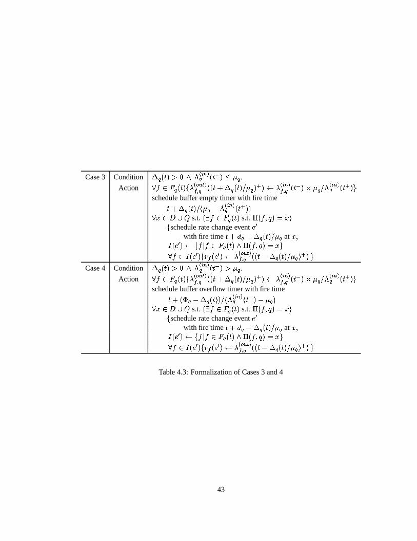
Case 3 Condition � � ��� � � 1 �� �� ��� 5 � � � .
Action� � �*� � ��� �� �"� �4# %'�� � � ����� � � ��� �� � � 5 � �"�
� �� � ���5 � � � �/1 �
� �� ���5 �
schedule buffer empty timer with fire time��� � � ��� �� ��� � � 1 �� �� ��� 5 � � �*� � � s.t. � � � �*� � ��� s.t. ( � � � � � � � schedule rate change event 8
with fire time ��� � � � � � ��� �� � � at � �7 �98 � � � � �)��� � ��� � ( � � � � � ��� � � 7 �98 �� � � �98 � � � �4# %'�� � � ��� � ������ �� � � 5 Case 4 Condition � � ��� � � 1 �
� �� ���5 � � � .
Action� � �*� � ��� �� � � �4# %'�� � � ����� ��� ��� �� � � 5 � � �
� �� � ��� 5 � � � �/1 �
� �� ��� 5 �
schedule buffer overflow timer with fire time��� � � � � � � ��� �� � 1 ����� ��� 5 ��� � � � �*� � � s.t. � � � �*� � ��� s.t. ( � � � � � � � schedule rate change event 8
with fire time ��� � � � � � ��� �� � � at � �7 �98 � � � � �)��� � ��� � ( � � � � � ��� � � 7 �98 �� � � �98 � � � �4# %'�� � � ��� � � � ��� �� � � 5 Table 4.3: Formalization of Cases 3 and 4
43

then equal to its arrival rate. Since some flows change their arrival rates, these rate changes shouldbe propagated to the next ports on their paths, or their destinations if they disappear into a sink, afterthe corresponding link latencies. Note that � in the action part can be a port or a destination node.
Case 2 applies when there is no backlog in the buffer and the aggregate arrival rate exceeds thelink bandwidth associated with the port. Then, according to the FIFO service discipline, all flowsshare the bandwidth in proportion to their arrival rates. Similarly, we need to schedule rate changeevents at the next ports on their paths, or their destinations if they disappear into a sink at the nexthop. In addition, since the aggregate arrival rate exceeds the link bandwidth associated with theport, the backlog keeps increasing; therefore, a buffer overflow timer is scheduled at the exact timewhen the buffer becomes full.
Case 3 applies when there is backlog in the buffer and the aggregate arrival rate does not exceedthe link bandwidth associated with the port. Under such circumstance, the backlog in the buffer doesnot grow. The traffic that arrives after time � but before the buffer becomes empty will be buffered;when it is served, all flows share the bandwidth in proportion to their arrival rates during the abovetime period. In addition, since the aggregate arrival rate does not exceed the link bandwidth asso-ciated with the port, a buffer empty timer is scheduled at the exact time when the buffer becomesempty. Note that if 1 �
���� ��� 5 is equal to ��� , the backlog does not change, so the fire time scheduled
for the buffer empty timer is actually in the infinite future. Similarly, we schedule rate change eventsat the next hops on the paths of the flows. A special case is that 1 �
� �� ��� 5 is equal to 0. When this
occurs, we only need to schedule a buffer empty timer with fire time ��� � � ��� �� ��� � ��1 �� �� ���5 .
Case 4 applies when there is backlog in the buffer and the aggregate arrival rate exceeds thelink bandwidth associated with the port. Under such circumstance, the backlog in the buffer keepsgrowing. The traffic that arrives after time � will be buffered, or lost after the buffer overflows;all flows share the bandwidth in proportion to their arrival rates during the above time period. Inaddition, since the aggregate arrival rate exceeds the link bandwidth associated with the port, abuffer overflow timer is scheduled at the exact time when the buffer becomes full. Similarly, weschedule rate change events at the next hops on the paths of the flows.
Now we discuss how to update the state variables when a buffer empty timer fires. Supposea buffer empty timer fires at time � . We update the departure rate of every flow to be exactly thesame as its arrival rate and schedule rate change events at the downstream ports correspondingly.We define the action as follows:
Action:� � �*� � ��� �� ��� �4# %'��! � ���5 � �"�
� �� � ���5 �� � s.t. � � � �*� � ��� s.t. ( � � � � � � � schedule rate change event 8� with fire time ��� � � at � �7 �98 � � � � �)�*� � ��� � ( � � � � � � � � � 7 �98 �� � � �98 � � � �4# %'��! � ��� 5 �
When a buffer overflow timer fires, we do not need to update the flow departure rates. A bufferoverflow timer can be used to generate some traffic loss signals for end-host applications that aresensitive to them (e.g., TCP protocol).
44

d dBPort qA
r
d dBPort qA
r2r
(1) t = 0 (2) t = d
d dPort qA B
r2r
0
d dPort qA B
r0
(3) t = 2d (4) t = 3d
d dPort qA B
r0
d dPort qA B
0
(5) t = 4d (6) t = 5d
Figure 4.3: Illustration of A Discrete Event Fluid FIFO Port
45

We use a simple example to explain the dynamics of a discrete event fluid FIFO port. It isillustrated in Figure 4.3. Both traffic source � and sink � are connected to port � with latency
�.
We ignore the packet transmission time. Source A emits rate � at time 0, rate�� at time
�, and rate
0 at time� �
. The buffer size in port � is���. At time
�, rate � from source � arrives at port � . Case
(1) applies: a rate change event carrying rate � is scheduled to fire at time� �
at sink � . At time� �
,rate
�� from source � arrives at port � , and Case (2) applies: a rate change event carrying rate � is
scheduled to fire at time ��
at sink � , and a buffer overflow event is scheduled at time� �
. At time��, rate 0 from source � arrives at port � . The scheduled buffer overflow timer is canceled and the
backlog is updated as ��. Then Case (3) applies: a buffer empty timer is scheduled to fire at time� �
. Note that it is a special case because the aggregate arrival rate into port � is 0. Hence, no ratechange event is scheduled at this time. At time
� �, the scheduled buffer empty timer at port � fires
and a rate change event carrying rate 0 is scheduled to fire at time ��
at sink B. This event finallyfires at the scheduled time.
4.2.2 Ripple Effect
Consider a rate change event arriving at port � . From Cases (2) and (4) discussed in the previoussection, we know that if the new aggregate rate into the port exceeds the link bandwidth associatedwith it, then for every flow traversing through port � , its departure rate must be updated and thenpropagated to the next hop (after some delay), and for every port on the machine at the other endpointof the link associated with port � , if it is on the path of any flow traversing through port � , theremust be a rate change event scheduled at that port. Moreover, if port � is congested, backlog isaccumulated in the buffer. From Cases (3) and (4) discussed in the previous section, we also knowthat whenever a rate change event arriving at a port with backlog, we have to update the departurerate of every flow traversing through the port and propagate it to the next hop. When the changes onthe departure rates are propagated to the downstream ports, they may also encounter congested portsand trigger new flow rate changes there. In a network where many ports are overloaded, the numberof flow rate changes may grow dramatically as simulation time elapses. Such a phenomenon iscalled “ripple effect” in some literature [61][80].
Ripple effect is inherent in any event-driven fluid-oriented simulation of networks which al-low bandwidth sharing among multiple flows. Besides FIFO service discipline, GPS (GeneralizedProcessor Sharing) [113] is another such example. Although GPS scheduling principle providesbandwidth isolation among flows because every flow is provided a guaranteed service rate, it iswork-conserving: if a flow does not consume all of its guaranteed service rate, the residual servicerate will be shared among other flows whose input traffic cannot be served by their guaranteed ser-vice rates. Owing to the possible bandwidth sharing among such flows, event-driven fluid-orientedsimulation of a network with GPS service discipline may also suffer the ripple effect.
We use a feed-forward network to illustrate the ripple effect. In this topology, there are 16 flows,from � � to � ��� . Flow �
(� � � � �
) traverses 3 ports; flow �
( � � � ���) traverses 2 ports; flow
�
(� � � � ���
) traverses 1 port. Apparently, no circular dependence is formed by these flows inthe topology. Such a topology is sometimes called a feed-forward network. Suppose that a changeoccurs to the arrival rate of flow � � into congested port A. Then the arrival rates of flows � � and � �
46

2f3f4f
6f
1f 2f
3f4f
5f
7f8f
5f
1f2f
6f
3f4f
7f8f
9f10f
11f12f
13f14f
15f16f
Port A
Port B
Port C
Port D
1f
Sink
Port E
Port F
Port G
Figure 4.4: A Feed-Forward Topology
into port B and the arrival rates of flows � � and � � change after some delays. If ports B and C arealso congested, these rate changes will be propagated further to ports D, E, F, and G, where flows��� , � � , ��� , and ��� join them as ones that undergo rate changes. Similarly, if ports D, E, F, and G arealso congested, there is a rate change event delivered to every flow’s destination.
From the perspective of simulation efficiency, ripple effect imposes adverse impact on the event-driven fluid-oriented traffic simulation. As we have seen from the above example, a single ratechange at an upstream port may trigger a chain of rate changes downstream in a network wherethere exist multiple congested ports. Such an explosion of flow rate changes may cause heavycomputation cost on processing these rate changes in the simulation.
It is possible that event-driven fluid-oriented traffic simulation that suffers severe ripple effect isoutperformed by its counterpart packet-oriented simulation. A thorough comparison between theirperformance in tandem queueing networks and feedback queueing networks is provided in [79].Both mathematical analysis and simulation results suggest that when the ripple effect occurs in thenetwork, the rate at which simulation events are generated in event-driven fluid-oriented simulationmay exceed that in the counterpart packet-oriented simulation. Recall that the motivation for event-
47

driven fluid-oriented simulation is to achieve better simulation efficiency by abstracting packet-leveldetails. If it is unable to provide the performance comparable to the packet-oriented simulation, thismotivation is undermined.
4.2.3 Rate Smoothing
In this section, we present a rate smoothing solution that provably mitigates the ripple effect in event-driven fluid-oriented traffic simulation. From the four cases when a rate change event is processedat a port, we have observed that once the departure rate of a flow from this port is updated, thenew rate is bound to appear at the next hop on the flow’s path after a delay. This delay is simplyderived as the sum of the insensitive latency of the port and the time needed to release the backlogaccumulated before the rate change event arrives. We call this delay an insensitive period of a flowrate change.
r1
r2r3
r4
r5
t5 t1t2t3t4
� � �� � �� � �
� �� �� �
� � � �� � � �� � � �� � � �
� � � �� � �� �� �� �
���
Port pPort qd
(1) Before rate smoothing
r5
t5 t1
r’1� � � � � � � � � �� � � � � � � � � �
Port pPort qd
(2) After rate smoothing
Figure 4.5: Rate Smoothing
It is possible that multiple rate changes of the same flow, after departing from a port, all appearin the insensitive period at some simulation time point. This is illustrated in Figure 4.5(1). There
48

is a flow that traverses from port � to port � . The insensitive latency from of port � is�. Suppose
at some time point, there are 5 flow rate changes that have departed from port q but are still in theinsensitive period. These rates are denoted as � � , � � , � � , � � , and � � , and their fire times scheduledat port � are � � , � � , � � , � � , and � � respectively. If we flatten the bumpy rates between the flow ratechanges whose fire times are � � and � � , as illustrated in Figure 4.5(2), then only 2 rate changes arenecessary. That is, the flow rate changes whose fire times are � � , � � , and � � at port � can be removedfrom the simulation. The rate change whose fire time is � � at port � is replaced with one with rate� � , where
� � � � � ��� � � � � �� � � ��� � � � � � � � ��� � ��� � �� � � ��� � � � � � (4.3)
Note that the total volume of traffic that arrives at port � does not alter at simulation time � � afterthe rates are smoothed. However, the number of flow rate changes is reduced by three.
Flow 1
1tt2tn
r1,2r1,n
r2,n
ri,n
rm,n
r1,j
ri,j ri,3
r2,2
rm,1
Flow 2
Flow i
Flow m
tj t3
Port q
Port p
Port p
Port p
1
2
3
d
Figure 4.6: Rate Change Matrix
In order to incorporate this idea, we need to modify the implementation in Section 4.2.1. Atevery port, we maintain a list of pending rate changes for each flow that traverses it. On the otherhand, rate changes that occur at the same time are concatenated across flows. Therefore, all thepending rate changes form a matrix-like structure as depicted in Figure 4.6. When processing arate change event that updates the departure rates of some flows, we create a new column with theappropriate fire time, and concatenate all the new departure rate changes together. When we add anew departure rate change for a flow, we check whether there are more than one flow rate changeswhose fire times are no larger than the new one’s in the matrix. If there are, we smooth the rates asdiscussed above and remove the rate changes that happen between the earliest one and the new one.In Figure 4.6, suppose that the column corresponding to fire time � � is newly added. Then we can
49

apply the rate smooth technique on flow�
and remove � � �
from the matrix; similarly for flow � , wecan smooth the rate between fire times � � and � � , and thus remove �
�from the matrix.
We introduce a rate change delivery timer, which recursively fires at the earliest occurence timeamong all rate changes in the matrix. When a rate change delivery timer fires, we process it asfollows. We put all the rate changes of flows that go to the same next port into a rate change event,and deliver that event to the corresponding port; that port processes this event instantaneously in thesame way as discussed in Section 4.2.1. If there are flow rate changes destined for the node at theother end of the link, we create a rate change event containing all these rate changes and deliver itto the destination node.
From the above description, we can easily obtain the following lemma:
Lemma 1 Consider any flow traversing through a port with an insensitive latency�. If the rate
smoothing technique is applied as described, there are at most 2 departure rate changes within anyperiod of
�units of simulation time.
Proof. We prove it by contradiction. If there are more than 2 departure rate changes within a period�
units of simulation time, these rate changes must appear in the rate change matrix simultaneouslyat some simulation time point. Based on the above description, they can be smoothed and only twoare left. This contradicts the assumption. �
With aid of Lemma 1, we can establish the upper bound on the total number of flow rate changesthat are received by network components in an event-driven fluid-oriented simulation. We use � � todenote the set that contains all the output ports along flow � ’s path. Recall that
� � is the insensitivelatency of port � .
Theorem 1 Consider an event-driven fluid-oriented traffic simulation. Let set � contain all thefluid flows in it, and let � be the simulation duration time. Then the number of rate changes observedby network components in the simulation is no greater than�
�/-/. �� -���� �� �� � � � (4.4)
where� � � is the smallest integer that is no less than x.
Proof: For any flow � in the network, the number of its departure rate changes from port � ( ����� � )that is observed at the next network component after port � is at most
� � � � � � � based on Lemma1. Then the number of departure rate changes observed by all the network components on flow � ’spath is at most � � -��� � � � � � � � . By aggregating over all the flows, we can derive the upper boundon the total number of rate changes observed by network components in the simulation as Formula(4.7). �
From Formula (4.7), we know that the upper bound is entirely dependent on the simulationduration time, the network topology and how flows are routed in the network. Therefore, with therate smoothing technique applied, it is ensured that uncontrolled exponential explosion of flow ratechanges cannot happen.
50

Figure 4.7: The POP-Level ATT Backbone
We use the ATT backbone1 , which is illustrated in Figure 4.7, to empirically study the perfor-mance and accuracy of the rate smoothing technique. The topology has 27 POPs (Point of Pres-ences), connected with 100Mbps links. In order to study the impact that link latencies have uponthe performance and accuracy of the rate smooth technique, we vary the link latencies in the experi-ments between 0.1 second, 1 second and 10 seconds. The buffer size in an output port is the productof the bandwidth and the propagation delay of the link associated with the port. For every pair ofPOPs, we use the MMFM model discussed in Section 4.1 to generate its ingress traffic. Therefore,there are 702 (
� ��� � �) fluid flows in total. Each source traffic model is modulated by a Markov
chain with two states: in the “on” state, the sending rate is a positive constant � , and in the “off”state, the sending rate is 0. The holding time in each state is exponentially distributed with the samemean that is 1 second. In the experiments, we adjust constant rate � in the “on” state to achievetwo levels of traffic intensity in the network, one having average link utilization � �� and the otherhaving average link utilization
����.
From the experiments, we collect how many flow rate changes have been received by networkcomponents. Note that a network component can be either a router or a flow sink. Figure 4.9(a)presents the relative reduction on the flow rate changes observed by network components when theunconstrained rate smoothing technique is applied as opposed to when it is not. It is clear thatwhen the link latency increases, the number of flow rate changes received by network componentsdecreases. This is obvious because a larger link delay leads to more flow rate changes that aresmoothed before they take effect at the receiving network components. Moreover, as the trafficintensity level in the network increases, the number of flow rate changes in the simulation alsoincreases because of congestion, causing the number of flow rate changes that are smoothed out toincrease. This explains the large gap between the number of flow rate changes under different trafficloads in Figure 4.9(a).
1http://www.ssfnet.org/Exchange/gallery/usa/index.html
51

The number of flow rate changes that are generated in an event-driven fluid-oriened traffic sim-ulation is an important factor in determining its performance. However, there are some other im-portant factors that cannot be ignored. In our implementation, for example, the performance is alsoaffected by the number of timer events fired in the simulation. A timer event is inserted into thefuture event list in the underlying simulation engine when a rate change delivery timer, a bufferoverflow timer, or a buffer empty timer is scheduled. In addition, a traffic source also needs toschedule simulation events to indicate its rate changes. All these suggest that the factors affectingthe overall performance of event-driven fluid-oriented traffic simulation are manifold. In Figure4.9(a), we also present the relative reduction on the execution time when the unconstrained ratesmoothing technique is applied as opposed to when it is not. The results tell us that the overall trendof the simulation execution time agrees well with that of the number of fluid rate changes observedby network components in the simulation, but under both traffic loads, the reduction on the totalsimulation execution time is less impressive than that on the number of fluid rate changes observedby network components.
The performance improvement from the rate smoothing technique has a cost. In order to studyhow the rate smoothing technique affects the accuracy of the simulation results, for every flow inthe topology, we collect the volume of traffic it has received within non-overlapping time intervalsof equal length � . In the following experiments, we set � to be 1 second. Let
� � � � or� �� � �
( � � ��� ���� � � �) denote the processes that characterizes the volume of traffic received by flow � ’s
destination within the � -th time interval. Then the average relative error on the volume of trafficreceived by flow � is defined as
�� � ��
��� � �� � � � � � �� � � �� � � �
�(4.5)
where�
is the total number of non-overlapping timer intervals. In the experiments mentioned laterin this section,
�is 3,600.
The overall measure of the relative error is obtained by averaging the above relative errors of allthe flows:
� � � �� � �� � �
��
�� � � �� � � � � � �� � � �� � � �
�(4.6)
where � � is the total number of fluid flows. In order to reduce the variance in this accuracy mea-sure, we adopt the common random number technique discussed in Section 2.6: when computinga sample of
, the same random numbers are used in the simulations that derive
� � � � and� �� � � .
In addition, we remove all the samples that are extremely small; otherwise, the unreasonably largerelative error of a single sample can cause a very high average relative error.
The experimental results are presented in Figure 4.9(b). It is evident that with larger link delays,more inaccuracy is introduced. For example, when the link delay is as large as 10 seconds, the rela-tive error measured by Formula 4.6 is higher than 300% mark. This suggests that the rate smoothingtechnique, if used without any constraint, may adversely affects accuracy, especially when the linkdelays are relatively large. On the other hand, as we mentioned above, a higher traffic intensity
52

level in the network makes it more possible that flow rate changes are smoothed in the simulation.Therefore, we observe the relative error measure corresponding to average link utilization 80% ishigher than that corresponding to average link utilization 50%. However, compared with link de-lays, the traffic intensity level imposes relatively smaller impact on the relative error measure. Thisis because a heavier traffic intensity level in the network also leads to more traffic received at theegress nodes within each time interval, thus reducing the relative error measure.
From the experimental results, we have realized that there exists a tradeoff between performanceand accuracy when deciding whether the rate smoothing technique should be used. In particular,when the link delays in the network are large, applying the rate smoothing technique without anyconstraint leads to high inaccuracy. This may not be acceptable under some circumstance. In orderto avoid this problem, we can put a time constraint when smoothing flow rate changes. Let � be thelongest time interval within which flow rate changes are allowed to be smoothed. In other words,we do not smooth rate changes at time scales beyond � . Selection of � reflects a tradeoff betweensimulation accuracy and efficiency. A larger � can bring better performance but may impair thesimulation accuracy to a larger degree.
With the constrained rate smoothing technique, the upper bound on the total number of flowrate changes received by network components in Formula 4.7 should be modified correspondingly.Consider port � of insensitive latency
� � and any flow � that traverses it. If the constrained ratesmoothing technique is applied, at most two rate changes are received at the next network compo-nent with any time period
� � � � � � � � . Therefore, we can establish the upper bound on the totalnumber of rate changes in the simulation as in Theorem 1.
Theorem 2 Consider an event-driven fluid-oriented simulation in which the constrained rate smoothtechnique is applied as described. Let set � contains all the fluid flows in it, and let � be the sim-ulation duration time. Then the number of rate changes observed by network components in thesimulation is no greater than �
�/-�. �� -� � �� �
� � � � � � � � � � (4.7)
where� � � is the smallest integer that is no less than x.
We redo the previous experiments by setting � to be 1 second. The simulation results arepresented in Figure 4.9. As before, the relative reduction on the simulation execution time when theconstrained rate smoothing technique is applied is less impressive than that when it is not. This stillsuggests that the number of fluid rate changes in the simulation is an important but not the only factorthat affects the overall simulation performance. Comparing the results obtained by unconstrainedand constrained rate smoothing techniques, we have made the following observations:
� When the link delays are 0.1 second, which is much less than time constraint � on ratesmoothing, the simulation results are hardly affected by whether rate smoothing is con-strained;
� When the link delays are 1 second, if rate smoothing is constrained, the relative error de-creases but the number of flow rate changes increases slightly. Recall that the insensitive
53

latency of a port includes both the link propagation delay and the transmission delay of a sin-gle packet. Hence, it is actually longer than 1 second. When no time constraint is imposed,the probability with which fluid rates are smoothed is higher than that when time constraintis imposed.
� When the link delays are 10 seconds, if the constrained rate smoothing technique is applied,the relative error drops significantly, but fewer flow rate changes are removed because of thetime constraint on rate smoothing. We also observe that as the insensitive latencies of portsexceed time constraint � , both the relative error due to rate smoothing and the reduction onflow rate changes remain relatively insensitive to the link propagation delays.
We conclude that the constrained rate smoothing technique, with a careful selection of timeconstraint � , provides flexibility in balancing accuracy and efficiency of event-driven fluid-orientedtraffic simulation. The decision on time constraint � is application-specific. One important factorthat should be taken into consideration is how end applications respond to the inaccuracy due to ratesmoothing in the network.
The key idea of rate smoothing technique is to exploit the insensitive latencies that flow ratechanges have to suffer when traversing through a link; if they are in the insensitive period simul-taneously, we can flatten the rates so that some rate changes can be removed from the simulation.However, there are some complications when the link under consideration crosses timeline bound-aries in parallel and distributed simulation (see Section 2.4.1).
� If optimistic synchronization protocol is used, the rate smoothing technique can work as usual.When a rate change delivery timer fires, we pack the rate change events created in the cor-responding action part into messages, carrying a proper firing time, and send them to thetimelines that contain the receiving network components. When a message carrying flow ratechanges arrives at the receiving timeline, if the time these flow rate changes are supposed tofire occurs earlier than the local clock time, the message is treated as a “strangler” event andthe receiving timeline rolls back to the time stamp that the message carries.
� If conservative synchronization protocol is used, the rate smoothing technique may not work.Note that in the rate smoothing technique, rate changes are held at the port from which theydepart until they take effect at the receiving network components. However, typical conser-vative synchronization protocols in network simulation exploit the link propagation delays aslookaheads and use them to predict whether it can be ensured that no events will arrive withinthese delays in the future. The rate smoothing technique violates the assumption on suchlookahead, and therefore, potentially causes causality errors. Hence, in parallel or distributedsimulation based on conservative synchronization principle, we deactivate the rate smoothingtechnique on every port that is associated with a link crossing timeline boundaries.
54

0
0.1
0.2
0.3
0.4
0.5
0.6
0.7
0.8
0.9
1
0.1 1 10
Rat
io (
with
rat
e sm
ooth
ing
/ with
out r
ate
smoo
thin
g)
Link propagation delay (sec)
rate changes, link util 50%rate changes, link util 80%
execution time, link util 50%execution time, link util 80%
(a) Ratio of flow rate changes and execution time (simulation with unconstrained rate smoothing /simulation without rate smoothing)
0
0.5
1
1.5
2
2.5
3
3.5
0.1 1 10
Rel
ativ
e er
ror
Link propagation delay (sec)
link util 50%link util 80%
(b) Relative error
Figure 4.8: Results on Unconstrained Rate Smoothing
55

0
0.2
0.4
0.6
0.8
1
1.2
0.1 1 10
Rat
io (
with
rat
e sm
ooth
ing
/ with
out r
ate
smoo
thin
g)
Link propagation delay (sec)
rate changes, link util 50%rate changes, link util 80%
execution time, link util 50%execution time, link util 80%
(a) Ratio of flow rate changes and execution time (simulation with constrained rate smoothing /simulation without rate smoothing)
0.05
0.06
0.07
0.08
0.09
0.1
0.11
0.12
0.13
0.14
0.1 1 10
Rel
ativ
e er
ror
Link propagation delay (sec)
link util 50%link util 80%
(b) Relative error
Figure 4.9: Results on Constrained Rate Smoothing
56

4.3 Integration with Packet-Oriented Flows
In this section, we discuss how to integrate fluid-oriented and packet-oriented flows at the same port.This is illustrated in Figure 4.10. The interaction between fluid-oriented and packet-oriented flowsis mutual: when they compete for both bandwidth and storage in the buffer, traffic represented byfluid-oriented models affects traffic represented by packet-oriented models and vice versa. Ideally,the resource allocation at the multiplexing point should be fair; that is to say, the behavior of thetraffic should be transparent to the way in which it is represented. In our approach, we model theeffect that fluid flows have on packet flows separately from the opposite effect. These models arediscussed in the following subsections.
Fluid rate changes
Packets Port
Figure 4.10: Integration of Packet And Fluid Flows
4.3.1 Effect of Packet Flows on Fluid Flows
At a port that handles traffic mixing packet flows and fluid flows, we treat the aggregate packet flowas a special fluid flow: it arrives at the port with an input rate that is equivalent to the aggregaterate of packet flows but immediately disappears into a sink after departing from the port. Withaddition of this special fluid flow, we are able to apply the event-driven fluid simulation as describedin Section 4.2.1 directly except that it is unnecessary to compute departure rates for the special fluidflow. The rate smoothing technique discussed in Section 4.2.3 can still be applied to mitigate theripple effect that occurs to regular fluid flows.
The remaining question, then, is how to estimate the arrival rate of the aggregate packet flow.An ideal estimation mechanism should satisfy the following principles:
� The estimated rate of the aggregate packet flow should be sufficiently accurate so that thecompetition for bandwidth and storage in the buffer between the aggregate packet flow andthe regular fluid flows is “fair”. Fairness here means that the final service rates and bufferoccupancy are relatively insensitive to the way in which the traffic is represented.
� The computation cost on estimating the rate of the aggregate packet flow should be as lowas possible. From this perspective, the naive solution that fluidizes each packet arrival withtwo rate changes, one corresponding to its starting bit and the other to its ending bit, is toocomputationally costly.
57

� The estimated rates of the aggregate packet flow should not change too frequently. In a con-gested port, frequent changes on the estimated rates lead to a lot of computation on derivingthe departure rates for regular fluid flows.
In order to estimate the input rate of the aggregate packet flow, we define an adjustable mea-surement window � . When a packet with
�bytes arrives at time � after no packet appears during
time interval [ � ��� , � ), we set the instantaneous rate of the aggregate packet flow as� ��� , and then
schedule a packet rate estimation timer that fires at time ����� . As simulation time elapses, otherpackets may arrive before the timer fires. We use � to denote the total number of bytes that arrivewithin time interval ��� � � ��� � . Then, when the packet rate estimation timer fires at time � ��� ,the instantaneous rate of the aggregate packet flow is updated as � ��� , and we decide whether toreschedule the packet rate estimation timer in the following way: if � is not zero, the packet rateestimation timer is rescheduled to fire after another measurement window elapses, or otherwise, thetimer is simply canceled. Note that when the rate of the aggregate packet flow changes, there existsa delay before it is detected by the above estimation method. The selection on the measurementwindow � reflects a tradeoff between accuracy and efficiency. If a larger measurement window isused, the packet rate estimation timer fires relatively less frequently, thus causing less computationcost, but the estimation method is less responsive to the rate changes of the aggregate packet flow.In the implementation, we use an adjustable measurement window. When the packet rate estimationtimer fires, the next measurement window spans the time for approximately � packet arrivals, basedon the current estimate on the rate of the aggregate packet flow. In addition, in order to avoid a toolarge or too small measurement window, an upper bound ����� and a low bound ���
� are imposed
on � . In brief, the measurement window � is updated as follows:
� ��� � � � � � � �� � � � � � � ���� � � � � � (4.8)
where ��� is the current estimate on the rate of the aggregate packet flow.
4.3.2 Effect of Fluid Flows on Packet Flows
Recall that in the implementation described in Section 4.2.1, each fluid port has a state variable tokeep the current backlog in the buffer. When mixed traffic representations are supported, we fluidizethe aggregate packet flow and the backlog is updated as if the aggregate packet flow is a regular fluidflow. Upon a packet arrival, the backlog as calculated can be used to determine whether the packetshould be dropped due to buffer overflow, and if there is enough vacancy in the buffer, how muchwaiting time this packet has to suffer.
However, as mentioned before, the rate estimation for the aggregate packet flow has some delayin responding to its rate changes. This may lead to inaccuracy in the backlog computation if the de-lay is very large. Since the backlog calculated in this way serves the purpose of making decisions onpacket dropping and computing queueing delays, the inaccuracy may be amplified. In our approach,therefore, a separate state variable is maintained to keep the current backlog from the perspective ofpacket flows. Let � � be this state variable at port � . We use another state variable, � 3 , to store thelast time when this backlog is updated.
58

Another observation is that while a packet is being served, traffic that has arrived during thisperiod time is accumulated in the buffer until the packet has fully departed from the port. Hence,we introduce a state variable � ��� � to denote the residual time the packet being served requires to getfully transmitted. We initialize � ��� � to be 0 in the simulation setup.
Backlog � � is updated whenever a rate change event fires. Suppose rate change event 8 fires atport � at simulation time � . We update backlog � � as in the following two cases:
� Case � � : � � � 3 � � ��� � . This means that at simulation time � , the last packet must havefully departed from port � . Then, the backlog changes differently between time intervals [ � 3 ,� 3 � � ��� � ) and [ � 3 � � ��� � , t). The traffic that arrives in the first one has to wait in the buffer,causing the backlog to increase, but in the second interval, the backlog may drain, accumulate,or remain unaltered, depending on the relationship between the aggregate arrival rate into theport and the link bandwidth associated with the port. Hence, we update the backlog at time �as follows:
� � ��� ��� � � � � � � � � � � �� � � ��� 3 � 1 ����� � ��� 3 5 � � ��� � � � 1 �
� �� � ��� 3 5 � � � � ��� � � 3 � � ��� � �
(4.9)Note that the backlog in the buffer should not be negative or exceed the buffer size. Aftercomputing the new backlog, we update � ��� � to be 0 and � 3 to be � .
� Case � � : � � � 3 � � ��� � . This means that at simulation time � , the last packet has not fully leftport � yet. Traffic that arrives after �� 3 has to wait in the buffer. Hence, we update the backlogas follows:
� � ��� ��� � � � � � � � � ��� 3 � 1 ����� � ��� 3 5 � ��� � � 3 � (4.10)
After computing the new backlog, we decrease � ��� � by � � � 3 and update � 3 to be � .Now we discuss how to handle a packet arrival into a port. Consider a packet with length � �
arrives at port � at simulation time � . First, we update the backlog in the buffer in the same way asprocessing a rate change event and let � ��� � decrease by � � � 3 . Based on the current backlog, we thenprocess the new packet as follows:
� Case � � : � � ��� � and � ��� � �
. In this case, there is no backlog in the buffer and nopacket is being served. Hence, the packet is served at the instant time when it arrives. We set� ��� � to be � � � � � , which is the transmission time of the new packet. The new packet does notsuffer any delay, and it departs from the port entirely at time ��� � � � � � .
� Case ��� : � � ��� � and � ��� � �
. In this case, there is no backlog in the buffer but a packetis being served by the port. Hence, the new packet has to wait until the previous one is fullyserved. We then put the new packet into the buffer by resetting � � ��� to be � � . The exacttime when the new packet fully departs from the port is � � � ��� � � � � � � � . That is to say, thenew packet leaves the port after the time for the packet currently being served to finish itstransmission plus its own transmission time.
59

� Case � � : � � ��� � and � � ��� �� � � � � � . In this case, there is backlog in the buffer, and
the new packet has to wait for the transmission of itself until this backlog drains completely.If there is a packet being served, it also has to wait for its residual service time. Moreover,there is enough vacancy in the buffer to accommodate the new packet. Then, we add � � tothe current backlog � � ��� . Similarly, the exact time when the new packet fully departs fromthe port is � ��� ��� � ��� � ��� �� � � (note that the transmission time of the new packet has alreadybeen counted because � � ��� includes � � ).
� Case � � : � � ��� � and � � ��� � � � � � � . In this case, the new packet cannot be served
at the instant time when it arrives at the port because there is backlog in the buffer. Further-more, the calculated backlog does not leave enough storage space to hold the new packet. Anaive solution is to simply drop the packet. This, however, does not conform to the realitybecause even at an overloaded port, there is some probability for a fraction of traffic to getinto the buffer. Let � � ��� and � � ��� denote the aggregate packet arrival rate and the instantfluid arrival rate at simulation time � respectively. When the newly arrived packet cannot beaccommodated in the buffer, we drop the packet with probability
� 3 � � � � � � � � � � ��� � �� � ��� �� � � ��� � (4.11)
The packet loss probability formed as above can be explained as follows. If the port is over-loaded when the packet arrives (i.e., � � ��� � � � ��� � � � ), the overloaded portion is dropped;otherwise, the packet is put into the buffer and the backlog is set equal to the buffer size. Inaddition, we ensure that the packet dropping probability is a nonnegative. From a lot of exper-imentation, though, we find that the packet dropping probability presented in Formula (4.11)is slightly lower than that in the equivalent packet-oriented simulation. Therefore, we add aconstant scaling factor to compensate for this difference. The packet dropping probability inour implementation is
� 3 � � � � � ��� � � � � � ��� � �� � ��� � � � ��� � (4.12)
where � is 0.9 in all the experiments discussed later.
An important problem with the packet dropping probability in Formula (4.12) is how to de-termine the current aggregate packet rate � � ��� . In section 4.3.1, we have given an approach toestimating the aggregate packet arrival rate for bandwidth allocation among packet flows and reg-ular fluid flows. In order to balance the computation cost and responsiveness to the rate change ofreal packet flows, in that method we have adopted an adaptive measurement window that spans thetime for a constant number of packet arrivals. If the packet rate measured in that method is appliedin Formula (4.12) for estimating packet loss probability, the packet loss probability behaves verysensitively with respect to the measurement window. If the window is relatively large, the real ag-gregate packet arrival rate may differ significantly from the current estimate and the derived packetdropping probability is imprecise. If an overly small measurement window is applied, not only highcomputation cost is required to measure the packet rate, but also the estimated packet rate may beunreasonably high, thus causing an overestimation of the packet loss rate.
60

In order to achieve a robust and accurate estimation on the current packet arrival rate, we applythe approach used in [135] to measuring the arrival rate of the aggregate packet flow in Formula(4.12). Suppose a packet of length � arrives at time � . Let �63 � � % be the time when the previous packetarrives. We use � 3 � � %� be the packet flow arrival rate estimated when the last packet arrived. The newpacket flow arrival rate is then estimated by
� � ���� � � � � 8 ��� � � � �
�� 8 ��� � �
� 3 � � %��
(4.13)
where � is the last packet interarrival time (i.e., � ��� 3 � � % ) and�
is a constant. Compared with theaforementioned window-based rate estimation method, this one is able to capture the most recentpacket arrival rate intantaneously (the first item on the right side of Equation (4.13)). On the otherhand, this approach also distinguishes itself from the normal exponential averaging method in whicha constant exponential weight is used. In [135], it has been observed that the normal approachbehaves relatively sensitive to the packet length distribution and the derived packet rate estimatediffers from the real rate by a factor. Instead, the approach with weight 8 ��� � �
avoids this problem.Some guidelines on selecting
�have been given in the same paper. For example,
�should be large
enough to dampen the effect that packet delay-jitters have on the estimation process; on the otherhand, a smaller
�responds better to the rapid packet rate fluctuations. In the experiments discussed
later, we let�
be 100 ms.
Note that the original approach is used to estimate the arrival rate of an individual flow. In such acontext, it is ensured that the packet interarrival time is at least no less than the packet transmissiontime. Therefore, the estimated rate of a flow never exceeds the bandwidth of the link associatedwith the input port where the packet flow arrives. However, our problem requires estimating theaggregate packet flow rate at an output port. It is thus possible that multiple packets arrive at anoutput port at the same time or within a very small time frame in the simulation, and the derivedestimate on the aggregate packet flow arrival rate is too high. In order to solve this problem, weestimate the aggregate packet flow arrival rate from each input port at every output port. It is thusguaranteed that the estimated rate of the aggregate packet flow from a particular input port doesnot exceed the bandwidth of the link associated with that port. In addition, packets may also beoriginated from the local machine. Hence, we also estimate the arrival rate of the packet trafficsent by the local machine. The aggregate packet flow rate estimate used in Equation (4.12) is thenobtained by summing the arrival rate estimates of packet-oriented traffic from the local machine andall the input ports.
4.3.3 Simulation Results
In this section we evaluate our model with simulation experiments. The topologies used in theseexperiments involve the classical “dumbbell” topology shown in Figure 4.11 and the more complexATT backbone network shown in Figure 4.7. Given a particular topology, we change some of itsconfiguration parameters or rates at which flows inject traffic into the network. The accuracy andperformance of our approach are studied under varied network configurations.
61

BA
Bottleneck port
Client
Client
...
Client
Client
Client
Server
Server
Server
...
Server
Server
Figure 4.11: Dumbbell Topology
4.3.3.1 Experiment 1: Dumbbell Topology with MMFM Traffic
In this part, we present the simulation results with the dumbbell topology depicted in Figure 4.11. Inthis topology, a set of clients are connected to router A and a set of servers are connected to routerB; router A and router B are directly connected by a bottleneck link. The links in the topologyare homogeneous – they have the same bandwidth and propagation delay. The buffer size at thebottleneck port is set to be the bandwidth-delay product of the bottleneck link.
We vary the number of client-server pairs in the topology. One set of experiments has 1 TCPstream, 1 UDP stream, and 10 background flows. In the TCP stream, the TCP client requests a fileof 5M bytes from the corresponding TCP server. After the TCP server has successfully deliveredthe requested number of bytes, the TCP client “sleeps” for an exponentially distributed period withmean of 5 seconds. After the off period, the TCP client initiates another transfer of the same file size.The process repeats itself until the simulation is over. In the UDP stream, the UDP client requests afile of 5M bytes from its peer server. When the UDP server receives the request, it transfers the file tothe client at a constant rate. In the experiments, we let the rate be equal to the 10% of the bottlenecklink bandwidth. In addition, when the request is initiated, the UDP client schedules a user timer,whose fire time is set slightly later than the time for the server to finish the data transfer. When theuser timer fires, the UDP client remains “silent” for an exponentially distributed period with mean of5 seconds. After the off period, the UDP client sends another file transfer request to its peer server.This process repeats itself until the simulation terminates. The background flows are unidirectionalfrom the servers to their peer clients. In the hybrid simulation, we use the MMFM traffic model togenerate fluid rates for each background flow. Each MMFM traffic source is an on/off process: inthe “on” period the source sends traffic at a constant rate, and in the “off” period it does not sendtraffic. We fix each MMFM traffic source’s emission rate in the on period to be 2Mbps; the meantimes of both the “on” state and the “off” state are 1 second. In the pure packet-level simulation, the
62

MMFM traffic model is replaced with an equivalent packet-oriented model which generates packetsat the same rates in its fluid-oriented counterpart. In the experiments, we vary the link bandwidthbetween 12.5Mbps, 20Mbps, and 50Mbps; correspondingly, the traffic loads contributed by thebackground traffic flow are 20%, 50%, and 80% of the bottleneck link bandwidth. We also vary thelink propagation latency between 5 ms, 50 ms, and 500 ms.
We measure the packet loss probability at the bottleneck port. Figure 4.12 describes the resultswith 95% confidence interval. The ranges are very small and we thus hardly see them in the figure.In the pure packet-level simulation, we collect the packet loss probabilities of foreground trafficflows (i.e., the TCP stream and the UDP stream). Hence, packet loss probabilities of the sameportion of traffic are compared between the pure packet-level simulation and the hybrid simulation.From the graph, we find that the packet loss probabilities from two simulation approaches matchclosely. When the bottleneck bandwidth is 12.5Mbps, the average relative error on the packet lossprobabilities is 4.7% with standard deviation 2.6%; when the bottleneck bandwidth is 20Mbps or50Mbps, the packet loss probabilities are close to 0, which makes the derived relative errors hardlymeaningful.
0
0.02
0.04
0.06
0.08
0.005 0.05 0.5
Packet loss probability
Bottleneck latency (sec)
bandwidth 12.5Mbps, hybridbandwidth 12.5Mbps, packet
bandwidth 20Mbps, hybridbandwidth 20Mbps, packetbandwidth 50Mbps, hybridbandwidth 50Mbps, packet
Figure 4.12: Packet Loss Probability under 10 Background Flows
Figure 4.13 gives the average goodput of TCP streams. The goodput of a TCP stream is de-fined to be the average number of bytes successfully delivered per simulation time unit using TCPprotocol. The average relative errors on the TCP goodputs corresponding to the bottleneck band-width are 20.9% with standard deviation 9.3% at 12.5Mbps, 6.6% with standard deviation 6.4% at20Mbps, and 0.14% with standard deviation 0.22% at 50Mbps. It is clear that a higher bottleneck
63

link bandwidth causes less errors. From Figure 4.12, we know that the packet loss probability on thebottleneck link is very small when its bandwidth is high, and therefore, the complicated congestioncontrol mechanism in TCP is seldom triggered. This explains the decreasing relative errors whenbottleneck bandwidth increases. In Figure 4.14, we present the results on the average round triptime for the TCP stream. An excellent agreement is achieved because the relative error on everysimulation configuration is below 1%.
1000
10000
100000
1e+06
1e+07
0.005 0.05 0.5
Average TCP goodput (bytes/sec)
Bottleneck latency (sec)
bandwidth 12.5Mbps, hybridbandwidth 12.5Mbps, packet
bandwidth 20Mbps, hybridbandwidth 20Mbps, packetbandwidth 50Mbps, hybridbandwidth 50Mbps, packet
Figure 4.13: TCP Goodput under 10 Background Flows
Figure 4.15 describes the simulation results on how much traffic has been successfully deliveredby the UDP protocol. It is clear that the pure packet-level simulation and the hybrid simulationproduce very close results. The relative error on every simulation configuration is less than 1%.
64

0.03
0.3
3
0.005 0.05 0.5
Average RTT (sec)
Bottleneck latency (sec)
bandwidth 12.5Mbps, hybridbandwidth 12.5Mbps, packet
bandwidth 20Mbps, hybridbandwidth 20Mbps, packetbandwidth 50Mbps, hybridbandwidth 50Mbps, packet
Figure 4.14: TCP Round Trip Time under 10 Background Flows
0.9
0.92
0.94
0.96
0.98
1
0.005 0.05 0.5
Delivered fraction of bytes with UDP
Bottleneck latency (sec)
bandwidth 12.5Mbps, hybridbandwidth 12.5Mbps, packet
bandwidth 20Mbps, hybridbandwidth 20Mbps, packetbandwidth 50Mbps, hybridbandwidth 50Mbps, packet
Figure 4.15: Delivered Fraction of UDP Traffic under 10 Background Flows
65

In the second set of experiments, we increase the number of both foreground and backgroundflows, but the ratio of the former to the latter remains the same as in the first set. In these experi-ments, there are 10 TCP streams, 10 UDP streams, and 100 background flows. The traffic patternof each TCP stream is unaltered. The traffic pattern of a UDP stream is also the same, except thatthe sending rate of each UDP server is only one tenth of the rate in the first set. Hence, the overallpeak traffic load on the bottleneck link contributed by UDP traffic is still 10% of the bottlenecklink bandwidth. Similarly, a background flow from a server to its peer client is also modeled by aMMFM model in the hybrid simulation, and a packetized MMFM model in the pure packet-levelsimulation; when an MMFM source is in the “on” state, its sending rate is 0.2Mbps. Therefore,the average traffic load of the background traffic on the bottleneck link is 20% at 12.Mbps, 50% at20Mbps, and 80% at 50Mbps.
As before, we measure the packet loss probability at the bottleneck port. The simulation resultsare depicted in Figure 4.16. The average relative errors corresponding to the bottleneck link band-width are 4.6% with standard deviation 0.3% at 12.5Mbps, 16.4% with standard deviation 3.0% at20Mbps, and 33.7% with standard deviation 8.5% at 50Mbps. We have noticed that the high relativeerror under high bottleneck link bandwidth results from the relatively small packet loss probabilityin this range.
0
0.1
0.2
0.3
0.4
0.5
0.6
0.7
0.8
0.005 0.05 0.5
Packet loss probability
Bottleneck latency (sec)
bandwidth 12.5Mbps, hybridbandwidth 12.5Mbps, packet
bandwidth 20Mbps, hybridbandwidth 20Mbps, packetbandwidth 50Mbps, hybridbandwidth 50Mbps, packet
Figure 4.16: Packet Loss Probability under 100 Background Flows
The average TCP goodputs under varied network configurations are described in Figure 4.17.The average relative errors corresponding to bottleneck link bandwidth are 16.45% with standarddeviation 6.8% at 12.5Mbps, 32.5% with standard deviation 16.1% at 20Mbps, and 16.5% with
66

standard deviation 3.3% at 50Mbps. Compared with the results under 10 background flows, therelative errors under 100 background flows are relatively higher. Note that although we scale thesending rate of the UDP servers and the background traffic flows so that they offer the same loads onthe bottleneck link, there is much heavier TCP traffic load on that link under 100 background flows.Because of the increased overall traffic load on the bottleneck link, TCP behaves more dynamicallywhen responding to the relatively higher congestion in the network. This explains the increasedrelative errors on TCP goodputs under 100 background flows. In addition, we also measure theround trip times of the TCP packets. The results are shown in Figure 4.19. The relative errorscorresponding to the bottleneck link bandwidth are 1% with standard deviation 0.8% at 12.5Mbps,0.4% with standard deviation 0.4% at 20Mbps, and 0.8% with standard deviation 0.9% at 50Mbps.Obviously, the two simulation approaches have achieved excellent agreements on the round triptimes.
10
100
1000
10000
100000
1e+06
1e+07
0.005 0.05 0.5
Average TCP goodput (bytes/sec)
Bottleneck latency (sec)
bandwidth 12.5Mbps, hybridbandwidth 12.5Mbps, packet
bandwidth 20Mbps, hybridbandwidth 20Mbps, packetbandwidth 50Mbps, hybridbandwidth 50Mbps, packet
Figure 4.17: TCP Goodput under 100 Background Flows
The accuracy results on UDP traffic under 100 background flows are presented in Figure 4.19.It depicts the successfully delivered UDP traffic in the simulation. The average relative errors cor-responding to the bottleneck link bandwidth are 3.2% with standard deviation 0.4% at 12.5Mbps,5.3% with standard deviation 1.2% at 20Mbps, and 1.3% with standard deviation 1.4% at 50Mbps.These results suggest a close match on this UDP flow metric between the hybrid simulation and thepure packet-oriented simulation.
The execution speedups of hybrid simulation over pure packet-level simulation under variednetwork configurations are depicted in Figure 4.20. From the results, we see that hybrid simulation
67

0.03
0.3
3
0.005 0.05 0.5
Average RTT (sec)
Bottleneck latency (sec)
bandwidth 12.5Mbps, hybridbandwidth 12.5Mbps, packet
bandwidth 20Mbps, hybridbandwidth 20Mbps, packetbandwidth 50Mbps, hybridbandwidth 50Mbps, packet
Figure 4.18: TCP Round Trip Time under 100 Background Flows
outperforms pure packet-level simulation under all configurations. The lowest execution speedupis 1.4, when there are 100 background flows and the bottleneck link has bandwidth of 12.5Mbpsand propagation latency of 5 milliseconds; the highest execution speedup, which is 90, occurs whenthere are 10 background flows and the bottleneck link has bandwidth of 50Mbps and propagationlatency of 500 milliseconds.
Now we discuss the impact that the network configurations have on the execution speedup ofhybrid simulation over pure packet-level simulation. When the bottleneck latency increases andother conditions are the same, the execution speedup gained from hybrid simulation also increases.Since the UDP traffic and the background flows are non-responsive, that is, they do not adapt to thenetwork condition dynamically, changes on bottleneck latency hardly affects their traffic. Rather,TCP traffic is sensitive to the round trip times of packets – its throughput is roughly inversely pro-portional to the average round trip time [92]. Therefore, increasing the bottleneck latency reducesthe fraction of packet-oriented TCP traffic in hybrid simulation; hence, it is able to achieve a higherexecution speedup against the pure packet-level simulation.
The effects of the varied bottleneck bandwidth on the performance gain from the hybrid simu-lation are mixed when other conditions are the same. First, as the bottleneck bandwidth increases,the packet loss probability at the bottleneck port decreases and thus more packet-oriented traffic isable to get through the port. From this perspective, the pure packet-level simulation should be out-performed by the counterpart hybrid simulation. Second, increasing the bottleneck bandwidth alsoincreases the fraction of packet-oriented foreground traffic. Recall that the offered load of UDP traf-
68

0.4
0.6
0.8
1
1.2
1.4
0.005 0.05 0.5
Delivered Fraction of Bytes with UDP
Bottleneck latency (sec)
bandwidth 12.5Mbps, hybridbandwidth 12.5Mbps, packet
bandwidth 20Mbps, hybridbandwidth 20Mbps, packetbandwidth 50Mbps, hybridbandwidth 50Mbps, packet
Figure 4.19: Delivered Fraction of UDP Traffic under 100 Background Flows
fic on the bottleneck link is 10 percent of its bandwidth. Furthermore, a relatively large bottleneckbandwidth reduces the packet loss probability at the bottleneck port; an increase on the throughputof TCP stream results because it is roughly inversely proportional to the square root of the packetloss rate [92]. Third, increasing the bottleneck bandwidth also affects the interaction between fluidflows and packet flows in the hybrid simulation. A low bottleneck bandwidth causes relatively morecongestion. Under congestion, changes on the aggregate packet flow rate trigger computation ofdeparture rates of fluid flows. On the other hand, heavy congestion also causes more packet losses,which demands more time on computing the packet loss probability as described in Equation (4.13)in hybrid simulation. These reasons result in mixed effects that varying bottleneck bandwidth im-poses on the performance gain from the hybrid simulation. In most cases, the first factor dominatesover the other two because the background flows contribute to the most significant fraction of thewhole traffic. However, some exceptions occur when the bottleneck latency is small. In this range,the last two factors play a more important role than the first one, and the effect of increasing thebottleneck bandwidth on the performance gain of hybrid simulation is therefore slightly negative.
When we increase the number of flows (both foreground and background flows) in the simula-tion, it is clear that the relative execution speedup achieved by hybrid simulation over pure packet-level simulation drops. Although we configure the network in a way so that the offered load on thebottleneck link from background flows and packet UDP flows is maintained at the same level, theTCP traffic load under 100 background flows is heavier than that under 10 background flows. Sincethe fraction of packet-oriented traffic in hybrid simulation is higher in the former case, lower relative
69

1
3
9
27
81
243
729
0.005 0.05 0.5
Speedup over packet-level simulation
Bottleneck latency (sec)
bandwidth 12.5Mbps, 10 flowsbandwidth 20Mbps, 10 flowsbandwidth 50Mbps, 10 flows
bandwidth 12.5Mbps, 100 flowsbandwidth 20Mbps, 100 flowsbandwidth 50Mbps, 100 flows
Figure 4.20: Speedup of Hybrid Simulation over Pure Packet-Level Simulation under DumbbellTopology
execution speedup can be achieved from hybrid simulation. On the other hand, the performance offluid-oriented traffic simulation depends on the number of flows. When there are 100 fluid-orientedbackground flows in the hybrid simulation, more computation workload is inevitably needed topropagate their flow rate changes than that when there are only 10 fluid-oriented background flows.All these explain the observation that the relative execution speedup of hybrid simulation over purepacket-level simulation diminishes as the number of flows in the network increases.
4.3.3.2 Experiment 2: ATT Backbone with MMFM Traffic
In this section, the realistic ATT backbone network depicted in Figure 4.7 is used to study theaccuracy and performance of our approach to handling mixed traffic representations. The back-ground flows in the topology are “all-to-all”: for every pair of routers in the topology, there existsa background flow whose ingress traffic is modeled by the MMFM source model. As in previousexperiments, the model is actually an on/off process; both the “on” state and the “off” state havemean duration of 1 second. The emission rate in the “on” state is the same for all the backgroundtraffic sources. We adjust this rate to achieve two average background traffic loads on each link,50% utilization and 80% utilization.
In the original topology, we attach an end host to every router. Every end host has installeda TCP client, a UDP client, a TCP server, and a UDP server on it. In each experiment setting,
70

every TCP client randomly chooses a TCP server from all the end hosts but itself, and requests afile transfer of size 5M bytes from the selected server. When the client receives the requested file,it remains “silent” for an exponentially distributed duration with mean of 5 seconds; after wakingfrom the “silent” period, it initiates another request to the same server it has chosen. The aboveprocess repeats until the simulation finishes. Similarly, in each experiment setting, every UDPclient randomly chooses a UDP server from all other end hosts and requests a file transfer of 5Mbytes from there. After receiving a request, a UDP server sends back the requested bytes at the rateof 5Mbps. When a UDP client sends out its request, it schedules a user timer which fires slightlylater than the time when the corresponding server finishes its transfer. When the user timer fires,the UDP client goes to the “silent” period, which also conforms to an exponential distribution withmean of 5 seconds.
We randomly generate 10 experiment settings, in which each TCP client randomly selects aTCP server and a UDP client randomly selects a UDP server. In every experiment, there are 27TCP streams and the same number of UDP streams, all represented with packet-oriented models.We measure the average goodput of the 27 TCP streams and the average delivered fraction of UDPtraffic throughout the simulation. The results with 95% confidence interval on the average TCPgoodputs are given in Figure 4.21. The x-axis represents the 10 experiment settings. The averagerelative errors corresponding to the average background traffic loads are 6.3% with standard de-viation 2.0% at 50% and 3.4% with standard deviation 1.7% at 80%. The results on the averagedelivered fraction of UDP traffic under the 10 experiment settings are given in Figure 4.22. The rel-ative errors corresponding to the average background traffic load are 0.6% with standard deviation0.3% at 50% and 0.9% with standard deviation 0.8% at 80%. All these results suggest that purepacket-level simulation and hybrid simulation produce well-matched results on the flow metricsdiscussed.
We present the relative speedup of hybrid simulation over pure packet-level simulation in Figure4.23. We run each experiment setting for 3600 seconds, and each simulation run is replicated for 10times. From the graph, we have observed that when the average background traffic load is 50% ofthe link bandwidth, the relative execution speedup is approximately 4; when the average backgroundtraffic load is 80% of the link bandwidth, the relative execution speedup is approximately 8. Thedifference between these two numbers can simply be explained as follows. If background trafficload in the network is heavier, then a relatively larger portion of the whole traffic is as fluid flows,which thus brings better relative speedup from the hybrid simulation.
The average execution times under two background traffic loads are given in Table 4.4. It isclear that the pure packet-level simulation cannot be accomplished in real time, but the hybrid sim-ulation is finished within less than half the real time. This suggests that pure packet-oriented trafficsimulation is inappropriate in cases where meeting real time constraint is of crucial significance.In addition, with increasing background traffic load, the execution time by hybrid simulation de-creases. This may be counter-intuitive because a higher fluid traffic load in the network usuallyleads to heavier congestion and thus more computation on fluid rate propagation. In the hybridsimulation, however, a higher background traffic load may cause more packet losses because ofcongestion, thus reducing the overall computation load from this perspective. The experimentalresults tell us that the simulation performance is affected by the latter factor to a heavier degree.
71

500000
1e+06
1.5e+06
2e+06
2.5e+06
3e+06
3.5e+06
4e+06
0 1 2 3 4 5 6 7 8 9
TC
P g
oodp
ut (
byte
s /s
ec)
Experiment setting
link util 0.5, hybridlink util 0.5, packetlink util 0.8, hybridlink util 0.8, packet
Figure 4.21: TCP Goodput under ATT Topology
Background Traffic Load Hybrid Simulation Pure Packet-Level Simulation
0.5 984.85 (sec) 4013.08 (sec)
0.8 639.92 (sec) 5193.92 (sec)
Table 4.4: Average Execution Time for Simulating ATT Topology
72

0.8
0.82
0.84
0.86
0.88
0.9
0.92
0.94
0.96
0.98
1
0 1 2 3 4 5 6 7 8 9
Del
iver
ed fr
actio
n of
UD
P tr
affic
Experiment setting
link util 0.5, hybridlink util 0.5, packetlink util 0.8, hybridlink util 0.8, packet
Figure 4.22: Delivered Fraction of UDP Traffic under ATT Topology
0
2
4
6
8
10
0 1 2 3 4 5 6 7 8 9
Spe
edup
ove
r pu
re p
acke
t-le
vel s
imul
atio
n
Experiment setting
link util 0.5link util 0.8
Figure 4.23: Speedup of Hybrid Simulation over Pure Packet-Level Simulation under ATT Topol-ogy
73

4.4 Hybrid Simulation of TCP Traffic
In Section 4.3, we have discussed how to integrate event-driven fluid-oriented traffic simulationand packet-oriented traffic simulation, and in the experiments, the non-responsive MMFM modelis used to generate traffic represented as fluid rate changes. In this section, we continue the discus-sion in the context of TCP traffic simulation. As a large portion of the current Internet traffic usesTCP, it is thus important to understand both how TCP responds to the dynamic network conditionsand how its traffic affects network dynamics. Simulation is a tool that is widely applied to achievethese objectives. It is, therefore, a meaningful undertaking to investigate how to accelerate simu-lation of TCP traffic. In this section, we discuss the possibility of using hybrid simulation, whichintegrates fluid-oriented and packet-oriented TCP models, to achieve performance improvement. Inthe hybrid simulation, we have implemented Nicol’s fluid-based TCP model [104][108], with somesimplifications in order to improve simulation efficiency.
4.4.1 Nicol’s Fluid Modeling of TCP
Prior to the description of Nicol’s Fluid-Based TCP model, a brief introduction to TCP’s flow con-trol and loss recovery mechanism provides necessary background knowledge. TCP’s flow controlmechanism is centered on a sliding congestion window, whose size is adapted to reflect the currentnetwork condition. A TCP agent works in one of two modes: slow start and congestion avoidance[54]. In the slow start mode, TCP sender increases its congestion window size by the size of thatdata segment after receiving every data segment acknowledged by the receiver. In a topology wherethe round trip time is large enough to accommodate the transmission of all data segments withina congestion window, the congestion window size doubles every round trip time. The continuinggrowth of congestion window size at an exponential rate may cause congestion in the network. Ifa packet loss is detected, or the congestion window size exceeds a threshold called mode transitionthreshold, TCP enters the congestion avoidance mode. In this mode, TCP increases its congestionwindow size much more slowly compared with how it does in the slow start mode: the conges-tion window size is expanded by only one data segment after the volume of data segments equal tothe current congestion window size has been acknowledged by the receiver. Hence, in a topologywhere the round trip time is large enough to accommodate the transmission of all data segments ina congestion window, the congestion window size increases by a single data segment every roundtrip time.
TCP’s response to congestion in the network is manifold. The simplest approach existing inall TCP variants is to use retransmission timers: if a packet sent out has not been acknowledgedwhen a retransmission timer scheduled for it fires, the packet is assumed to be lost in the networkand TCP reacts as follows: it sets its mode transition threshold as half of the current congestionwindow size and its congestion window size as a single data segment, then re-enters the slow startmode. Relying on only retransmission timeouts for loss recovery, sometimes, severely limits thethroughput of the TCP traffic, especially in a network that is only slightly congested. Hence, afast retransmission mechanism [56] is adopted in many TCP variants. In this mechanism, whenmore than three duplicate acknowledgement packets are received in a row, a packet is assumed to
74

be dropped by the network. However, TCP variants differ in how to recover from packet lossesdetected from a fast retransmission. TCP Tahoe reacts to such a packet loss in the same way as thatafter a retransmission timeout. In TCP Reno, a fast recovery mechanism [55] is introduced: aftera fast retransmit, TCP reduces its current congestion window size by half and uses new incomingduplicate ACKs to expand its congestion window size; after half a window of duplicate ACK packetsare received, it increases the congestion window size by one MSS (Maximum Segment Size) andtransmits a data segment after each additional ACK packet is received. Besides TCP Tahoe andTCP Reno, other variants like TCP New-Reno and SACK further aim to improve the performanceof TCP protocol under varied circumstances. Among all these variants, TCP Reno is the mostwidely deployed because it has been implemented in the popular BSD 4.3 operating system. All theexperiments in this thesis regarding packet-oriented TCP protocol use the Reno variant.
In the following paragraphs, we introduce Nicol’s fluid modeling of TCP from three aspects:how to update the emission rate from the TCP sender, how to schedule timers, and how to respondto packet losses in the network.
4.4.1.1 Sending Rates
In Nicol’s fluid-based TCP model, a data transfer governed by TCP protocol is abstracted into a fluidstream of bytes, indexed from 0 in byte sequence order. At the TCP sender side, two state variablesregarding the current transfer status are maintained:
� � � ��� and� ��� ��� keep the number of bytes
that have been sent and the number of bytes that have been received respectively up to simulationtime � . It is obvious that at any simulation time
� � � ��� should be no less than� � � ��� . We
have mentioned that TCP’s flow control mechanism is centered on its sliding congestion windowand the mode transition threshold. Their values at simulation time � are denoted by ��� �
� ��� and� � � � � 8 � � ��� respectively.
Similar to the MMFM traffic model, Nicol’s fluid-based TCP model also injects discrete fluidrate changes into the network. Let � � � ��� ��� be the data rate sent from the TCP sender at simulationtime � , and � � ! � ��� be the acknowledged byte rate received from the network at simulation time � .Both � � � ��� ��� and � � ! � ��� are piece-wise constant rate functions of simulation time � . One importantgoal of the model is to determine � � � ��� ��� , that is, the data transmission rate from the TCP sender.First, if the current congestion window is not filled (i.e.,
� � � ��� � � � � ��� � ��� �� ��� ), the
TCP sender can send out data as fast as it can. The maximum emission rate is constrained byboth the data rate from the upper application, denoted by � � �� ��� , and the available transmissionbandwidth, denoted by ��� � ��� . Second, when the congestion window size is tight (i.e.,
� � � ��� �� � � ��� � ��� �
� ��� ), the sending rate is further contingent on both � � ! � ��� , and the rate at whichthe congestion window size increases. The latter is denoted by � ! � ��� ��� . As we have said, the TCPsender increases its congestion window size differently in two modes. In slow start, the congestionwindow size increases by one MSS after one data segment has been acknowledged. Therefore, therate at which the congestion window changes in this mode is equal to the rate at which data segmentsare acknowledged. That is to say, � ! ����� ��� is exactly � � ! � ��� . If the TCP sender is in congestionavoidance mode, we simply let � ! ����� ��� be 0, because as we will see later, the congestion windowsize is changed in a discontinuous manner. Third, it is possible that the current congestion window
75

size is smaller than� � � ��� � � � � ��� . This may occur when the TCP sender shrinks its congestion
window size after some packet losses have been detected. In this case, the sending rate is constrainedto be 0. In summary, the rule on updating � � � ��� ��� is described as follows:
� � � ��� ��� ��������� �������
� � � � � � � ��� � � � �� ��� � if � ��� �� � � �� ���
� � � � � � � ��� � � � �� ��� � � � ! � ��� � � ! ����� ��� � if � ��� � � � �� ���
if � ��� �� � � �
� ��� (4.14)
where � ��� is equal to� � � ��� � � ��� ��� .
4.4.1.2 Timers
A few timers are necessary for updating the internal state variables in the model. The first oneis called Constrained timer. It is scheduled when the congestion window size is unfilled (i.e.,� � � ��� � � � � ��� � ��� �
� ��� ). The purpose of this timer is to notify when the congestion win-dow becomes full. From Equation (4.14), we know that the data transmission rate may need to bechanged when the entire congestion window is filled. Suppose that the timer is scheduled at time � .Its fire time, � ! , is then � ! � ��� � � �
� ��� � � � � ��� �� � � � ��� � � � ��� ��� � � � ! � ��� � � ! ����� ��� � (4.15)
When the Constrained timer fires at time � , the sending rate � � � ��� ��� is updated according to thesecond case in Equation (4.14).
Another timer called ModeTransition timer is responsible for mode transition from slow startto congestion avoidance. It is scheduled only when the TCP sender is in slow start mode. Whenscheduled at simulation time � , its fire time is
� � � ��� � � � � � 8 � � ��� � ��� �� ���
� ! � ��� ��� �(4.16)
As mentioned before, the congestion window size is changed discontinuously in congestionavoidance mode. A timer called IncreaseCWND timer is used to notify when the congestion windowsize should be increased. Let � # � � ! � ��� be the amount of unacknowledged data in the congestionwindow since its size changes last time in congestion avoidance mode. Note that the first time thecongestion size changes in congestion avoidance mode is when TCP transmits from slow start modeto congestion avoidance mode. This timer, when scheduled at time � , is to fire at time
� � ��� � # � � ! � ��� � � ! � ��� �
(4.17)
In order to avoid firing the IncreaseCWND frequently, an optimization is employed in the model.The timer is only running when
� � � ��� � � � � ��� � ��� �� ��� because otherwise it does not affect
76

the data transmission rate � � � ��� ��� based on Equation (4.14). But the current congestion windowsize needs to be known when the Constrained timer is scheduled. It can be reconstructed as follows.Let � be the congestion window size when TCP enters the congestion avoidance mode. Supposethat at the point of calculation, 1 bytes have been acknowledged since the mode transition fromslow start to congestion avoidance. We then solve the following equation:
1 � � � � ��� � � � � ��� � � �� ��� (4.18)
Let � be the positive solution to the above equation. The current congestion window size is thenreconstructed as
��� �� � � ��� � �� � � � � � (4.19)
where � � � is the largest integer that is no greater than �� .4.4.1.3 Loss Recovery
TCP has an adaptive mechanism for responding to packet losses in the network. Nicol’s fluid model-ing of TCP takes it into consideration as well. In order to analyze lost bytes in the fluid stream, fluidrate changes carry extra information, including the delivered fraction and flow position components.The delivered fraction indicates the fraction of the raw fluid traffic that is successfully delivered;hence, the loss rate of the raw fluid flow can be easily inferred. Flow position components provideinformation on the current byte sequence that is being delivered. From such information fed backto the TCP sender along with the ACK flows, the amount of lost traffic can be inferred. It is thenpossible to model the fast retransmit logic in TCP. Besides fast retransmit, Nicol’s fluid TCP modelalso considers retransmission timeouts. The TCP agent fires the retransmission timer every 500milliseconds. It computes the time at which the current acknowledged byte sequence (i.e.,
� � � )was transmitted. If that is earlier than the last time the retransmission timer was fired, all the bytesin the current congestion window are retransmitted.
We have discussed Nicol’s fluid modeling of the TCP sender. The behavior of the counterpartTCP receiver is relatively simple. One of its primary tasks is to transform the received data byterates into the acknowledgment byte rates. There may be some discrete information that needs to bepassed in a flow. For example, when the TCP sender wants to terminate a flow, it needs to notify thecorresponding receiver of it. Such information is carried in extra data structures called corks. Whena TCP receiver receives a cork, it simply pass it back along with the ACK flow.
4.4.2 Modifications
In some cases, we need to simulate many TCP flows but the high-fidelity behavior of only a smallnumber of them are of interest to us. In such circumstance, we can use a hybrid model to simulateTCP traffic. The TCP flows whose packet-level characteristics are being studied can be representedwith packet-oriented models. We can represent the remaining TCP flows with Nicol’s fluid TCPmodel to improve the simulation efficiency. As said in Section 4.4.1, Nicol’s fluid TCP model cap-tures rich details of real TCP behavior, including both its window-based flow control mechanism
77

and its retransmission logic. At the same time, it provides some optimizations to improve its effi-ciency, such as “lazily” updating the congestion window size when the TCP agent is in congestionavoidance mode. However, we need to make some modifications on it in the hybrid simulation.First, its modeling of TCP’s response to packet losses, if detected by fast retransmit logic, is com-plicated. Furthermore, in order to implement the retransmission timeouts, this model requires thatevery TCP agent be interrupted every 500 milliseconds to check whether it is necessary to retrans-mit the entire congestion window. Therefore, although Nicol’s model is loyal to the behavior of thereal TCP protocol, it can still be simplified to achieve better simulation efficiency. Since the behav-ior of the fluid-oriented TCP traffic is not of our interest in the hybrid simulation, a precise modelcharacterizing very details of TCP protocol is unnecessary. The bottom line is that the fluid-basedTCP model is able to generate the background traffic that is accurate enough for packet-orientedTCP traffic.
From a lot of experimentation, however, we know that the fluid TCP model, if simplified in animproper way, results in significant “unfairness” between fluid-oriented and packet-oriented TCPtraffic. For example, if we totally ignore retransmission timeouts in the fluid model and any packetloss detected causes TCP to re-enter transmission mode immediately, then after some congestionoccurs on a bottleneck link that packet-oriented and fluid-oriented TCP flows share on their paths,fluid TCP traffic exhibits more aggressive behavior and the packet-oriented TCP flows may thus ob-tain much less throughput than they should have. On the other hand, totally ignoring fast retransmitis also problematic. Suppose that in the fluid-based TCP, any lost byte is retransmitted when theretransmission timeout occurs. Then in a lightly congested network where most of packet lossesare recovered by fast retransmit in reality, packet-oriented TCP flows may obtain a much higherthroughput in the hybrid simulation than what they do in pure packet-level simulation.
We have also made another observation from the experiments. This occurs when many fluid-oriented TCP flows traverse through the same congested bottleneck port. Given the FIFO policyas described in Section 4.2.1, the lost traffic spans over every fluid-oriented TCP flow that has apositive input rate. When losses are detected by the corresponding fluid TCP senders, they shrinktheir congestion window sizes in a way that depends on how they respond to the lost traffic. In thepure packet-level simulation, however, some TCP flows may be so “lucky” that their packets are notdropped when the congestion occurs at the port. If the congestion lasts long enough, these flows maystill suffer packet losses, but at a time later than when the congestion starts at the port. Therefore,the fluid-oriented TCP agents in hybrid simulation decrease their congestion window sizes earlierthan the packet-oriented TCP agents do in pure packet-level simulation. We call this observationearly window reduction syndrome. Note that this problem is rooted from the continuous feature ofthe fluid FIFO port, and thus irrelevant of whether a full-fledged fluid TCP model is adopted. Thisphenomenon may cause unfairness between packet-oriented and fluid-oriented TCP flows in hybridsimulation. The packet-oriented TCP flows may not suffer losses as the congestion starts. Thenfluid-oriented TCP flows deflate their congestion window sizes, leaving packet-oriented TCP flowsthe opportunity of inflating their congestion windows up to a higher size than in the equivalent purepacket-level simulation.
All the above observations lead us to establish an empirical model on how a fluid-based TCPagent recovers from lost bytes. When the buffer in a port overflows, a special signal is sent to
78

every fluid-based TCP flows that traverses that port. When such a signal arrives at a TCP sender,say at time � , it immediately strangles existing flows. That is to say, the transmission rate � � � ��� ��� is changed to 0. Unlike the original model, the new model eliminates the necessity of detectingwhen loss finishes. Rather, it sends a special cork, called loss clearance cork, along with the latestrate change (i.e., rate 0). This cork traverses through the network, reaches the corresponding TCPreceiver, and is finally passed back to the TCP sender. Suppose the cork is returned to the TCPsender at time � . Let �!3 � � � be the difference between
� � � ��� and� � � ��� :
� 3 � � � � � � � ��� � � ��� ��� � (4.20)
It is clear that � 3 � � � is the number of lost bytes because no traffic is sent out since time � . A heuristicsis applied here to decide whether the lost traffic is detected by retransmission timeout or fast retrans-mit by a real TCP protocol. If more packets in the same congestion window have been dropped inthe network, it is relatively less likely that the packet losses can be recovered from the fast retransmitand fast recovery mechanism in TCP Reno, and thus more possibly, lost packets are retransmittedwhen the retransmission timer fires. If only slight congestion occurs in the network, it is relativelylikely that the packet losses are recovered from the fast retransmit and fast recovery mechanism.Based on such heuristics, we use the following rule to decide the way in which the lost traffic isretransmitted: if �!3 � � � is larger than a MSS, lost bytes are recovered at retransmission timeouts, orotherwise, they are recovered from fast retransmit and fast recovery mechanism. With this heuris-tics, if the network is only slightly congested and some fluid TCP flows thus mistakenly receivetraffic loss signals from the network, they are able to recover their original congestion window sizesafter only a few round trip times, instead of suffering the long retransmission timeouts and the slowstart phase.
In the modified model, we do not fire the retransmission timer every 500 milliseconds. Rather,a retransmission timer is scheduled by a TCP agent only when the recovery from some lost trafficattributes to retransmission timeouts. If a loss clearance cork arrives at the TCP sender and � 3 � � �is found to be greater than a MSS, a retransmission timer is scheduled to fire after a particulardelay � � � 8 ��� � . Then, it comes to how to calculate � � � 8 ��� � . The TCP protocol derives theretransmission timeout with the following equations [28]:������������ �����������
� 7 � � � � � � � �98 � � � � � � � � � �
� � � �/� � 8 � � � � � � � � � � ��� $ � � 7 � �� � � � � � � � � � � � � 7 � � � � � � � � � � � � 8 ��� � � � � � �/��� 8 � � � �&��� � � �
(4.21)
where � � � � �98 � � � is the sampled RTT, � � � � � � is the old estimate on the mean of RTT,� � � �/��� 8 � � � � is the new estimate on the mean of RTT, � � � � �
is the old estimate on the stan-dard deviation of RTT, � �
is the new estimate on the standard deviation of RTT, and � � � 8 ��� � isthe retransmission timeout. In 4.4 BSD Unix, $ , � , and � are 1/8, 1/4, and 4 respectively. In order
79

to obtain an approximate estimate on � � � 8 ��� � in the fluid-based TCP model, the TCP sender needsto sample the current RTT. This is done by sending RTT sampling corks along with rate changes.When such a cork is sent, the TCP sender notes down the simulation time at that moment. There isat most one RTT sampling cork on the fly. That is to say, before a RTT sampling cork already sentout is returned to the TCP sender, no other RTT sampling corks are sent. When a RTT samplingcork is passed back to the TCP sender, the RTT is estimated by the difference between the currentsimulation time and the time when the cork was sent. Equation (4.21) can then be applied to com-pute the current retransmission timeout. However, recall that rate smoothing technique may smoothout the rate change with which a RTT sampling cork is associated. In order to prevent the compli-cations involved in correcting such errors, a policy is added at every FIFO port that smoothing outany rate change that carries a RTT sampling cork is forbidden.
When the retransmission timer fires after � � � 8 ��� � , the mode transition threshold � � ��� � 8 � � isset to be half of the congestion window size, and the congestion window size ��� �
�is set to be one
MSS. In order to retransmit the lost bytes,� � � is simply set equal to
� ��� .
As a loss clearance cork is returned to the TCP sender, �/3 � � � is calculated as Equation (4.20).If � 3 � � � is less than a MSS, then the TCP sender applies the fast retransmit logic: shrink the modetransition threshold � � � � � 8 � � to be half of the current congestion window size, set the congestionwindow size ��� �
�to be � � � � � 8 � � plus 3 MSSes, and set the mode to be congestion avoidance. In
order to retransmit the lost bytes,� � � is set equal to
� ��� .
4.4.3 Simulation Results
The dumbbell topology depicted in Figure 4.11 is used to study the accuracy and performance of thehybrid simulation of TCP traffic. Every link in the topology has the same bandwidth and propagationlatency. Two sets of experiments are designed. In the first set of experiments, we use 10 TCP clientsand 10 TCP servers. Each TCP client requests a file transfer of 5M bytes from its peer server;After a client receives all the requested bytes from the counterpart server, it keeps “silent” for anexponentially distributed period with mean of 5 seconds. In the second set of experiments, thereare 100 TCP clients and 100 TCP servers; the traffic pattern of every client-server pair is the sameas in the first set of experiments. In each set of experiments, we vary the link bandwidth between5Mbps, 50Mbps and 500Mbps; we also vary the link propagation latency between 5 ms, 50 msand 500 ms. Therefore, each set of experiments has 9 configurations. The simulation length ofeach configuration is 3600 seconds. We use the hybrid simulator and pure packet-level simulator tosimulate each configuration independently.
In the hybrid simulation, we represent 20 percent of TCP flows with packet-oriented modelsand the other 80 percent of TCP flows with fluid-oriented models. Therefore, in the first set ofexperiments, 2 TCP flows are modeled as packet-oriented TCP and 8 TCP flows as fluid-orientedTCP; in the second set of experiments, there are 20 packet-oriented TCP flows and 80 fluid-orientedTCP flows. In the simulation, we are interested in packet-level TCP statistics like TCP goodputand round trip times. We also consider network statistics like average packet loss probability at thebottleneck port. The relative speedup of the hybrid simulation over the pure packet-level simulationis also studied because it offers us insights into the performance gain from the fluid-oriented TCP
80

model used in the hybrid simulation.
4.4.3.1 Accuracy
As we will see later from the simulation results, when there are many TCP flows traversing throughthe same bottleneck port, the behavior of each individual TCP flow is dynamic, causing the collectedsamples, except the round trip times, to exhibit high variation. Hence, it is difficult to quantify theaccuracy of the statistics collected from the hybrid simulation using methods like relative errors.Instead, we focus on whether the results collected from the hybrid simulation are reasonable. Iftheir mean falls within the range in which the samples are collected from the pure packet-levelsimulation, the results are viewed as totally reasonable; otherwise, the distance that it is from thatrange suggests how reasonable it is.
0
0.01
0.02
0.03
0.04
0.05
0.005 0.05 0.5
Packet loss probability
Bottleneck latency (sec)
bandwidth 5Mbps, hybridbandwidth 50Mbps, hybridbandwidth 500Mbps, hybridbandwidth 5Mbps, packetbandwidth 50Mbps, packetbandwidth 50Mbps, packet
Figure 4.24: Packet Loss Probability under 10 TCP Flows
Statistics on average packet loss probabilities, TCP goodputs, and round trip times are describedin Figures 4.24-4.29. From the simulation results, we have observed that in most cases the hybridsimulation and the pure packet-level simulation achieve excellent agreement on all collected statis-tics, but there is a visible discrepancy on average packet loss probability and TCP goodput whenthe bottleneck bandwidth is the lowest. The exception can be explained as follows. If the bottle-neck bandwidth is higher, there is less mutual interaction between packet-oriented and fluid-orientedtraffic at the bottleneck port, thus reducing the impact of any error caused by the model integratinghybrid traffic as discussed in Section 4.3. On the other hand, if the bottleneck link bandwidth is
81

10000
100000
1e+06
1e+07
1e+08
0.005 0.05 0.5
Average TCP goodput (bytes/sec)
Bottleneck latency (sec)
bandwidth 5Mbps, hybridbandwidth 50Mbps, hybridbandwidth 500Mbps, hybridbandwidth 5Mbps, packetbandwidth 50Mbps, packetbandwidth 500Mbps, packet
Figure 4.25: TCP Goodput under 10 TCP Flows
lower, the congestion level at the bottleneck port becomes higher and more bytes are thus lost fromthe fluid-based TCP streams. As discussed in Section 4.4.2, the fluid-based TCP model’s response tolost traffic is a heuristics-based approximation to the real TCP’s behavior. Increasing the congestionlevel thus increases the likelihood that higher errors result from that loss recovery model.
A closer examination reveals that the hybrid simulation overestimates the packet loss probabilitywhen the bottleneck port is under heavy TCP traffic load. For example, when the bottleneck latencyis 5 milliseconds, the average packet loss probability in hybrid simulation is higher than the highestpacket loss probability that an individual TCP stream suffers in the pure packet-level simulation,regardless of the number of TCP flows in the simulation. The phenomenon results from the earlywindow reduction syndrome mentioned in Section 4.4.2. If the congestion level at the bottleneckport is very high, all the fluid TCP flows suffer either retransmission timeouts or fast retransmitafter some congestion is detected at the bottleneck port. In either case, the congestion windowsizes of some fluid TCP flows deflate earlier than they should. This allows some packet-orientedTCP flows to inflate their congestion windows up to a higher size than that in the pure packet-level simulation. Therefore, it is observed from the simulation results that in the region of lowlink bandwidth and low bottleneck latency, hybrid simulation produces higher average packet-levelTCP goodputs than pure packet-level simulation. This seems to contradict the higher packet lossprobabilities observed in hybrid simulation. Actually, because packet-oriented TCP flows are ableto reach a higher congestion window size, the burstiness of their traffic results in more TCP packetsbeing dropped at the bottleneck port in later rounds.
82

0.03
0.3
3
0.005 0.05 0.5
Average RTT (sec)
Bottleneck latency (sec)
bandwidth 5Mbps, hybridbandwidth 5Mbps, packetbandwidth 50Mbps, hybridbandwidth 50Mbps, packet
bandwidth 500Mbps, hybridbandwidth 500Mbps, packet
Figure 4.26: TCP Round Trip Time under 10 TCP Flows
Although the hybrid simulation overestimates the packet loss probabilities at the bottleneck portunder heavy load, most of the TCP goodputs observed from the simulation results are feasible.In addition, the hybrid simulation also predicts well the average round trip times of TCP packets.Regardless of the number of TCP flows in the network, the relative error on this metric is below4.0% under every network configuration.
In summary, the simulation results tell us that our hybrid model works fairly well under lightand medium TCP traffic load in the network. But when the TCP traffic load in the network is high,the hybrid model is prone to overestimate the packet loss probability at the bottleneck port, butstill produces feasible predictions on the average TCP goodputs and round trip times. However, formany applications whose behavior is sensitive to TCP statistics not network statistics, our hybridmodel provides a good solution.
4.4.3.2 Execution Speedup
In this section, we discuss the relative execution speedup of the hybrid simulation over the purepacket-level simulation. Note that all the TCP flows are homogeneous. Hence, we can establishthe upper bound on the execution speedup. Let ������� �
� be the total execution time of the hybrid
simulation. It consists of three parts:
����� � ��� � � � ! � �$% � � � 3 # � � �
� % � � � !9% � � (4.22)
83
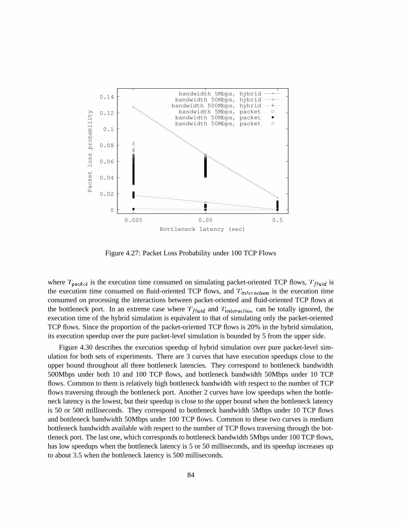
0
0.02
0.04
0.06
0.08
0.1
0.12
0.14
0.005 0.05 0.5
Packet loss probability
Bottleneck latency (sec)
bandwidth 5Mbps, hybridbandwidth 50Mbps, hybridbandwidth 500Mbps, hybridbandwidth 5Mbps, packetbandwidth 50Mbps, packetbandwidth 50Mbps, packet
Figure 4.27: Packet Loss Probability under 100 TCP Flows
where � � � ! � �$% is the execution time consumed on simulating packet-oriented TCP flows, � � 3 # � isthe execution time consumed on fluid-oriented TCP flows, and �
�/% � � � !9% � � is the execution time
consumed on processing the interactions between packet-oriented and fluid-oriented TCP flows atthe bottleneck port. In an extreme case where � � 3 # � and �
� % � � � !9% � � can be totally ignored, the
execution time of the hybrid simulation is equivalent to that of simulating only the packet-orientedTCP flows. Since the proportion of the packet-oriented TCP flows is 20% in the hybrid simulation,its execution speedup over the pure packet-level simulation is bounded by 5 from the upper side.
Figure 4.30 describes the execution speedup of hybrid simulation over pure packet-level sim-ulation for both sets of experiments. There are 3 curves that have execution speedups close to theupper bound throughout all three bottleneck latencies. They correspond to bottleneck bandwidth500Mbps under both 10 and 100 TCP flows, and bottleneck bandwidth 50Mbps under 10 TCPflows. Common to them is relatively high bottleneck bandwidth with respect to the number of TCPflows traversing through the bottleneck port. Another 2 curves have low speedups when the bottle-neck latency is the lowest, but their speedup is close to the upper bound when the bottleneck latencyis 50 or 500 milliseconds. They correspond to bottleneck bandwidth 5Mbps under 10 TCP flowsand bottleneck bandwidth 50Mbps under 100 TCP flows. Common to these two curves is mediumbottleneck bandwidth available with respect to the number of TCP flows traversing through the bot-tleneck port. The last one, which corresponds to bottleneck bandwidth 5Mbps under 100 TCP flows,has low speedups when the bottleneck latency is 5 or 50 milliseconds, and its speedup increases upto about 3.5 when the bottleneck latency is 500 milliseconds.
84
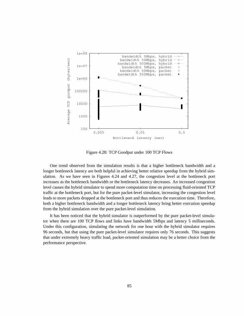
100
1000
10000
100000
1e+06
1e+07
1e+08
0.005 0.05 0.5
Average TCP goodput (bytes/sec)
Bottleneck latency (sec)
bandwidth 5Mbps, hybridbandwidth 50Mbps, hybridbandwidth 500Mbps, hybridbandwidth 5Mbps, packetbandwidth 50Mbps, packetbandwidth 500Mbps, packet
Figure 4.28: TCP Goodput under 100 TCP Flows
One trend observed from the simulation results is that a higher bottleneck bandwidth and alonger bottleneck latency are both helpful in achieving better relative speedup from the hybrid sim-ulation. As we have seen in Figures 4.24 and 4.27, the congestion level at the bottleneck portincreases as the bottleneck bandwidth or the bottleneck latency decreases. An increased congestionlevel causes the hybrid simulator to spend more computation time on processing fluid-oriented TCPtraffic at the bottleneck port, but for the pure packet-level simulator, increasing the congestion levelleads to more packets dropped at the bottleneck port and thus reduces the execution time. Therefore,both a higher bottleneck bandwidth and a longer bottleneck latency bring better execution speedupfrom the hybrid simulation over the pure packet-level simulation.
It has been noticed that the hybrid simulator is outperformed by the pure packet-level simula-tor when there are 100 TCP flows and links have bandwidth 5Mbps and latency 5 milliseconds.Under this configuration, simulating the network for one hour with the hybrid simulator requires96 seconds, but that using the pure packet-level simulator requires only 76 seconds. This suggeststhat under extremely heavy traffic load, packet-oriented simulation may be a better choice from theperformance perspective.
85

0.03
0.3
3
0.005 0.05 0.5
Average RTT (sec)
Bottleneck latency (sec)
bandwidth 5Mbps, hybridbandwidth 5Mbps, packetbandwidth 50Mbps, hybridbandwidth 50Mbps, packet
bandwidth 500Mbps, hybridbandwidth 500Mbps, packet
Figure 4.29: TCP Round Trip Time under 100 TCP Flows
0
1
2
3
4
5
6
7
8
0.005 0.05 0.5
Speedup over packet-level simulation
Bottleneck latency (sec)
bandwidth 5Mbps, 10 flowsbandwidth 50Mbps, 10 flowsbandwidth 500Mbps, 10 flowsbandwidth 5Mbps, 100 flowsbandwidth 50Mbps, 100 flowsbandwidth 500Mbps, 100 flows
Figure 4.30: Execution Speedup of Hybrid Simulation over Pure Packet-Level Simulation
86

4.5 Related Work
The ripple effect associated with event-driven fluid simulation has been observed in early work onfluid simulation such as [61]. In [79], an approach to dampening ripple effect is described. Inthe method, flows in a network are combined into fewer aggregate flows. Hence, when the inputrate of the aggregate flow changes, only one rate change is propagated to the downstream networkcomponent. The viability of this solution is contingent on two premises. On one hand, flows beingaggregated must be destined for the same place; otherwise, when an aggregate flow splits intomultiple destinations, we are unable to restore the rate change destined to a particular destinationfrom the aggregate flow. On the other hand, the destination of each flow should not respond to therate changes it receives in the simulation. Otherwise, if a fluid flow uses a responsive protocol likeTCP, aggregating it into a larger flow in the network inevitably loses its detailed flow rate changeinformation needed by the corresponding end application.
In [63], an alternative solution called fluid threshold policy is proposed to mitigate ripple effect.In this method, a new departure rate of a flow is propagated to the next network component onlyif it differs from the old departure rate by a percentage higher than a given threshold. In otherwords, if the two consecutive departure rate changes corresponding to the same flow are very closeto each other, the one that occurs later in simulation time is ignored. This solution disobeys theflow conservation principle, which dictates that after a flow traverses through a lossless network,the destination should receive exactly the same amount of traffic as the source has sent out after afinite delay in simulation time. If the fluid threshold policy is applied as described, the destinationmay receive less or more than what the source has sent out. Hence, this method makes it difficult toimplement some volume-aware applications like large file transfers unless the network provides theerror information to the end applications. In addition, as pointed out by the author, errors derivedfrom this method can propagate through the network. An error that happens at a port is embodied inthe arrival rate at the next hop, where it may cause further errors due to the fluid threshold policy. In anetwork where a flow suffers errors at multiple ports on its path, the accumulated error at its receivermay be significant. Finally, in contrast to our rate smoothing technique, the fluid threshold policylacks a strict upper bound on the number of rate changes that are received by network componentsin event-driven fluid simulation.
There are a few examples that integrate packet-oriented and event-driven fluid-oriented trafficsimulation into the same network simulator. In [126], integration of fluid-oriented and packet-oriented network simulations is considered. The HDCF-NS (Hybrid Discrete-Continuous FlowNetwork Simulator) [93], which models behavior of fluid flows with discrete events, is used to gen-erate fluid-oriented background traffic for the packet-oriented foreground traffic simulated with thepdns simulator2 . The two simulators simulate the same topology simultaneously in separate addressspaces, and the fluid-oriented background traffic simulation, as it evolves, updates the buffer occu-pancy in the packet-oriented foreground traffic simulator. In contrast to our approach, their methoddoes not consider the impact that packet flows have on fluid flows. It thus eliminates the necessity ofestimating flow rates for packet-oriented traffic, as is needed in our approach. The accuracy of theirapproach is contingent on the premise that the packet-oriented foreground traffic can be ignored
2http://www.cc.gatech.edu/computing/compass/pdns/index.html
87

when competing for bandwidth and buffer storage with fluid-oriented background traffic. If thepacket-oriented foreground traffic is significant as opposed to the fluid-oriented background traffic,the communication bandwidth allocated to fluid flows will be overestimated.
The work in [64][63] bears some similarities to ours. The integration of fluid-oriented andpacket-oriented traffic is done in the IP-TN simulator [130]. It also models the mutual interactionbetween fluid-oriented and packet-oriented traffic when they multiplex at the same port. In thismethod, a single state variable is used to keep the current buffer occupancy at each port, and thisvariable has dual purposes: determining the queueing delay when a packet arrives at the port anddetermining the fire time of fluid departure rate changes spawned by a fluid input rate change. Thisdiffers from our approach which uses two separate variables, one serving for each of the abovepurposes. Although our approach brings more complication to the implementation, it reduces thenegative impact that the errors resulting from packet rate estimation impose on the calculation ofbuffer occupancy. In their approach, the packet arrival rate is estimated by summing the sizes of thelast � packets and then dividing the sum by the time interval in which these packets arrive. Underextreme cases, the estimation approach may suffer significant inaccuracy. For example, if the last �packets arrive from � different input ports at the same time in the simulation, the time interval is 0and the packet rate estimate is infinitely large. This conforms to the observation we have made fromour own experiments: estimating packet rate is a delicate process and it may make the simulationresults very sensitive to the parameter settings. In our approach, we use separate methods to esti-mate packet rates, one for competing bandwidth and the other for computing dropping probability,because from a lot of experiments we have done, it is observed that the accuracy of the simulationresults is less sensitive to the former than the latter, especially when the fluid-oriented traffic is adominant portion of the overall traffic.
4.6 Summary
In this chapter, we have discussed event-driven fluid-oriented traffic simulation and its integrationwith packet-oriented traffic simulation. There are some fluid-oriented traffic sources like MMFMand fluid-based TCP that generate fluid rate changes at discrete times. When fluid rate changes frommore than one source multiplex at the same port in the network, they affect each other’s departurerates if the port is overloaded. In a network where there exist multiple congested ports, “rippleeffect” may occur in event-driven fluid-oriented traffic simulation, causing explosion of fluid ratechanges in it. We have proposed a rate smoothing technique to mitigate “ripple effect”. The key ideaof this approach is that it exploits the insensitive latency of a port when fluid rate changes traversethrough the associated link so that rate changes corresponding to the same flow within a short timeinterval can be flattened. We noticed that unconstrained rate smoothing may cause too much errorto the simulation results, an adjustable time constraint on this technique offers a tradeoff betweenaccuracy and efficiency.
We also have presented an approach to integrating fluid-oriented and packet-oriented trafficsimulation in the same discrete event simulator. In our model, both the effect that packet-orientedtraffic has on fluid-oriented traffic and the effect vice versa have been modeled. We have done
88

some experiments, using the MMFM model to generate fluid-oriented traffic. From the simulationresults, close agreements have been observed between the hybrid simulation and the counterpartpure packet-oriented simulation. We have also seen execution speedups at varying orders from thehybrid simulation over the pure packet-oriented simulation.
Finally, we have studied the accuracy and performance of hybrid TCP traffic simulation. Nicol’sfluid-based TCP model has been modified to generate fluid-oriented traffic bearing TCP character-istics. From the simulation results with the dumbbell topology, we conclude that under light andmedium traffic load, the hybrid simulator is able to achieve both reasonable accuracy results andgood execution speedups against the pure packet-level simulator, but under heavy traffic load, thehybrid simulator is prone to overestimate the packet loss probability and can possibly be outper-formed by the pure packet-level simulator.
89

Chapter 5
Time-Stepped Coarse-Grained TrafficSimulation
In Chapter 4, we have seen that event-driven fluid-oriented traffic simulation is able to achievesignificant execution speedup over pure packet-level traffic simulation. Such performance gainresults from the capability of fluid-oriented representations to abstract packet-level details withincertain time scales. As the time scale of interest becomes coarser, flow rate changes can further beaggregated in the time domain, making event-driven time advancement inefficient.
Motivated by this observation, a time-stepped technique is proposed in this chapter to simulatenetwork traffic at coarse time scales. It periodically updates the demand discharged by each fluid-oriented traffic source. At every time step, traffic is assumed to converge to a steady state in thenetwork within a relatively short time as opposed to the time scale being considered. This eliminatesthe necessity of using discrete events to propagate new rates through the network; instead, theaggregate traffic load on each link is directly computed with an optimized algorithm. In order toachieve further scalability, the algorithm is parallelized on a distributed memory multiprocessor.The PPBP traffic model, which exhibits self-similarity observed in various types of networks, isused to generate the traffic demands for each fluid-oriented traffic source.
The remainder of this chapter is organized as follows. Section 5.1 discusses the motivationbehind the time-stepped coarse-grain traffic simulation. In Section 5.2, the outline of our solution isprovided. In Section 5.3, we formulate the problem to be investigated. In Section 5.5, a sequentialalgorithm is presented, followed by a discussion on its convergence behavior, performance andaccuracy. In Section 5.7, we describe how to parallelize the sequential algorithm on a distribuedmemory multiprocessor; simulation results on the scalability of the parallel algorithm with bothfixed and scaled problem size are also presented. Section 5.8 discusses how to modify the algorithmin a network that implements the GPS service discipline [113]. In Section 5.9, some related work isdiscussed. Section 5.10 summarizes this chapter.
90

5.1 Background
The motivating application for time-stepped coarse-grained traffic simulation is the RINSE (Real-Time Immersive Network Simulation Environment) project, which provides a real-time networksimulation platform for cyber-security exercises and training [75]. Owing to human participationin RINSE, the underlying network simulator must run as fast as real time. Therefore, it poses asignificant performance challenge to the simulator. The traffic in a network simulation can breakdown into two parts. Foreground traffic is the part whose behavior is of essential interest to the user,and background traffic is the part that itself is not concerned by the user but may affect the behaviorof foreground traffic. For example, when RINSE is used to study how malicious worm traffic affectsthe ongoing financial transaction services, the transaction traffic is treated as foreground traffic.
In network simulation, background traffic usually constitutes a large fraction of the networktraffic, or in many cases most of the network traffic. Hence, it is not a trivial problem to simulatebackground traffic efficiently in a real-time simulation environment like RINSE. The simplest wayof simulating background traffic is to use a random traffic generator to generate the backgroundtraffic load on each link. This approach, although efficient and scalable, loses spatial correlationamong background traffic on different links.
The ( � � � � � ) model [89] is a WAN (Wide Area Network) background traffic generation model.In its first phase, the FGN (Fractional Gaussian Noise) model [8], a self-similar traffic model, is usedto generate a sequence of aggregated traffic traces from every traffic source in the network. Such asequence is called an aggregate stream. In the second phase, an aggregate stream is decomposedinto individual substreams, one for each destination campus network access point, by samplingsome probability models. In the final phase, the packet-train model discussed in Section 2.2.2 isapplied to convert each of these substreams to short-term packet arrivals. Although the ( � � � � � )model achieves execution time savings because of the aggregated traffic stream per source campusnetwork, the large number of packets generated after the final phase can make it difficult to satisfythe real time constraint.
An alternate way of simulating background traffic is using fluid-oriented models. Since TCPtraffic dominates the current Internet traffic, fluid-based TCP models can be exploited to improvebackground traffic generation as observed in Chapter 4. However, modeling traffic in a large net-work at session level is still an arduous undertaking because of the enormous TCP sessions in it. In[85], a fluid-based TCP model using stochastic differential equations, combined with a time-steppedtime advancement mechanism, is applied to simulate a ring topology with 1,045 nodes. The experi-mental results show that simulating 176,000 TCP flows in this network for 100 seconds takes about74 minutes, which is far from real time.
5.2 Solution Outline
Since existing background generation methods are unable to satisfy the real time constraint requiredin RINSE, a time-stepped coarse-grained traffic simulation technique is developed to achieve thisobjective. Aggregation, a strategy often adopted to simplify simulation models (See Section 2.2.1),
91

is the key idea. In the space domain, all flows that traverse between the same source-destination pairare aggregated and treated as a single aggregate flow in the simulation. In a large network, usuallymany sessions between an ingress-egress pair use the same path. Under such circumstance, the flowaggregation technique can significantly reduce the number of flow states and thus the computationcomplexity. On the other hand, aggregation is also applied in the time domain. Simulating large-scale background traffic at fine time scales is computationally costly, but is sometimes unnecessarywith regard to the simulation objective. Our approach, driven by constant time steps, simulates thenetwork traffic at coarse time scales. At every time step, a new traffic matrix that contains trafficdemands among all ingress-egress pairs is generated. The traffic demand between an ingress-egresspair is assumed to be unaltered between any two successive time steps. The transient behavior thatoccurs before the whole network traffic converges to a steady state is ignored because of the coarsetime scale considered. Hence, this technique numerically computes the background traffic load oneach link given the current traffic matrix, and this load remains unchanged until the next time step.
The relationship between foreground traffic simulation and background traffic computation isillustrated in Figure 5.1. Background traffic can affect how foreground traffic behaves. As men-tioned before, after the background traffic computation at a time step, a background traffic load iscalculated on every link in the network. It is this load that imposes impact on the foreground traf-fic traversing on the same link. Actually, from the perspective of foreground traffic, the aggregatebackground traffic traversing through a port can be viewed as a virtual event-driven fluid-orientedflow that immediately disappears into a virtual sink after departing from the port. Moreover, thisvirtual flow periodically updates its arrival rate as the background traffic load at this port computedat every time step. This virtual flow competes for bandwidth and buffer space with foreground traf-fic as if it were a regular event-driven fluid-oriented flow. In this way, background traffic can shapethe behavior of foreground traffic.
On the other hand, foreground traffic can also affect background traffic. This conforms to theprinciple that traffic behavior should be transparent to the way in which traffic is represented inthe simulation. If foreground traffic is as intense as background traffic, ignoring its impact onbackground traffic may introduce significant inaccuracy to the simulation results. In our approach,when the background traffic load on a link is computed, the volume of foreground traffic that it has“seen” since the previous time step is collected. Moreover, it is assumed that between the currenttime step and the next time step, the same amount of foreground traffic will traverse on this link.This simple model may not predict the real foreground traffic closely. It, however, can be easilyreplaced with a more powerful but more complicated prediction model like ARIMA (AutoregressiveIntegrated Moving Average) traffic model [10]. When we compute the background traffic load atan output port, it is assumed that there exists a virtual aggregate flow, which comes from the routerassociated with this port, crosses the link, and then immediately disappears into a sink; at every timestep, this virtual aggregate flow injects an ingress rate that is equal to the total volume of foregroundtraffic seen since the previous time step divided by the time step size. Therefore, our approach alsocaptures the impact of foreground traffic on background traffic in the simulation.
92

Simulation time
Simulation event generated forforeground traffic simulation
Background traffic computation
Figure 5.1: Relationship between Foreground Traffic Simulation and Background Traffic Computa-tion
5.3 Problem Formulation
In the time-stepped traffic simulation, the simulation time is discretized into units of length � , andwe use �� to denote ��� � ( � � �� ��� ���� � �
). We assume that the network being studied consists of �
POPs, denoted by� � , � � , ...,
� � . We use � �
to represent the aggregate flow between ingress-egresspair � �
� � � � . For any ingress-egress pair � �
� � � � (
� � � ��� � � ), we use � � ��� to denote
ingress rate of the corresponding aggregate flow at time � . Since the simulation time advances byconstant time intervals, we need to discretize the ingress rate for every aggregate flow. During thetime interval [ �� , �4� 5 � ], the traffic volume emitted from ingress node
�
to egress node� �
is
� %����%�� � � ��� d � � (5.1)
We smooth the burstiness at time scales smaller than � . In order to ensure that the same amountof traffic is injected into the network, the ingress rate of aggregate flow �
�at discretized time ��� �
is �
� �� % ���% � �
� ��� d � � (5.2)
The network is modeled as a collection of routers connected with uni-directional links. Thesending endpoint of a link is associated with a router’s output port. At an output port, there is anoutput buffer. We assume that every router adopts the output buffering strategy, although we under-stand that other buffering strategies can be easily incorporated with minor modifications. Routingprotocols are used to direct traffic for each aggregate flow. The routing decisions are assumed tobe static within any discretized time interval. In addition, the time step size � is relatively largewith respect to the typical end-to-end latency of an aggregate flow. Therefore, all link latencies areassumed to be zero in the network model.
93

Let set � denote the whole set of output ports in the network. The sequence of output ports anaggregate flow �
�traverses at discretized time � � is denoted by � ��� � � ���4� . Obviously, � ��� � � ��� � is a
subset of � . � � ���4� is used to denote the whole set of aggregate flows that traverse port � ( ��� � ) at
discretized time � � . We use �"�� �� � ��� � ( � � � � ��� � ) to denote the arrival rate of aggregate flow � at
output port � at discretized time ��� . The sum of all the arrival rates into port � , � ��-/.�0 � % � � � �� �� � ��� � ,
is written as 1 �� �� ��� � . In addition, we use
�� � ��� � to denote the ingress rate of aggregate flow �
from its traffic source at discretized time � � .When multiple aggregate flows traverse the same output port, the bandwidth is allocated to each
is governed by the port’s queueing policy. Consider an output port � with the FIFO queueing policy.Let � � denote the link bandwidth associated with � . According to the FIFO service discipline, the
departure rate of flow � ( � ��� � ��� � ) at discretized time �� , denoted by � � �$#&%'��! � ��� � , is as follows:
� � �4# %'�� � ��� � � � ����� � ���4� � min � ��� � �1 �
� �� ��� � � (5.3)
When the aggregate arrival rate does not exceed the link bandwidth, the output port can serve allinput traffic; otherwise, congestion occurs and traffic that cannot be served has to be dropped; theFIFO queueing policy dictates that the loss that occurring to each flow be proportional to its arrivalrate. In Equation (5.3), we do not model the queueing delay, and therefore, there is no time shiftbetween the departure rate and the arrival rate. This is a reasonable assumption because a coarsetime scale is being considered.
As discussed in Section 5.2, one objective is to compute the aggregate traffic load at each port:
� ��-/. 0 � %�� � �"�� �� � ��� � for every ��� � � � (5.4)
For some applications, the egress rate of each aggregate flow needs to be reported to its sink.For example, the emission rate of an aggregate flow at a time step may be a function of the rate atwhich the ingress node receives traffic from the network at the previous time step. Hence, anotherobjective is to compute the aggregate egress rate from each POP. In order to formulate this objective,we introduce another notation. We define function ( � � � � , where �)� � � ��� � , as follows:
( � � � � ����� ��� � if � ( � � � ) is the next output port on flow � ’s path after leaving port ��
if flow � arrives at its destination�
(� �)� � ��� � � ) after leaving port �
(5.5)
We formulate the second objective as computing�� -� �/-�. 0 � %�� � � � � � � � �
�$#&%'��! � ��� � � for every�
:� � � � ��� � � � (5.6)
94

5.4 Solutions in Specific Settings
Given the problem formulated in Section 5.3, we introduce three types of networks and discuss howto solve the problem on these networks. Some examples are presented to help us understand thecharacteristics of the problem under varied settings.
5.4.1 Networks with Sufficient Bandwidth
We define a network with sufficient bandwidth as one in which the bandwidth associated with anylink is no less than the sum of the ingress rates of all the flows that traverse on it. It is worthy ofnoting that a network with sufficient bandwidth does not necessarily have high-bandwidth links; alow-bandwidth network, if little traffic traverses through it, can still be deemed as a network withsufficient bandwidth. Networks with sufficient bandwidth are not uncommon in the Internet. Inorder to avoid deploying complicated QoS mechanisms, many network operators prefer to over-provision link bandwidth in their networks. This renders it possible that congestion seldom occursin such networks. Moreover, after a new network is deployed, its traffic load is usually very low fromthe beginning. Such a network at its initial operational stage can also be deemed to have sufficientbandwidth. It is thus meaningful to discuss how to solve the problem formulated in Section 5.3efficiently when the traffic load is so low that no congestion occurs in the network.
In a network with sufficient bandwidth, the solution can actually be very simple. Becauseno congestion should happen in the network, every flow is able to push all its traffic towards itsdestination without any loss. The aggregate traffic load at each output port can be simply calculatedby adding the ingress rates of all the flows that traverse it. Hence, the aggregate traffic load at eachport can be computed as �
�/-�.�0 � % � ��� � ��� � for every ��� � � � � (5.7)
Similarly, the egress rate at a POP can be computed by adding the ingress rates of all the flowsthat are destined to it. At POP
�(� �)� � ��� � � ), its aggregate egress rate is�� -�� �/-�.�0 � % � � � � � � �
�� � ��� � � (5.8)
For each flow that traverses in the network, the above solution reads or updates the state of everyport on its path for a constant number of times. If we use � and � to denote the total number offlows in the network and the average number of ports on a flow’s path, then the time complexity issimply ��� � � � .
5.4.2 Feed-Forward Networks with Limited Bandwidth
When the links in a network have limited bandwidth, it is likely that some of them are congestedbecause the limited bandwidth cannot serve all the input traffic. The topology discussed in this
95

example is the feed-forward network shown in Figure 4.4. As we mentioned in Section 4.2.2, nocycle is formed in this network.
After the setup of every time step, we know the ingress rate from each flow’s source. It isobserved that at port A, the arrival rates of all the flows that traverse it are already known. Therefore,the departure rate of flow �
(� � � � �
) from port A can be determined using Equation (5.3). Wesay that we resolve a port if we use Equation (5.3) to compute the departure rates of all the flowstraversing through it after all their arrival rates are known. After port A is resolved, the arrival ratesof flows � � and � � into port B are known, and the arrival rates of flows � � and � � into port C are alsoknown. Thereafter, we can further apply Equation (5.3) on ports B and C in an arbitrary order. Onceport B is resolved, we know the arrival rates of flows � � and � � into port D, and the arrival rates offlows � � and � � into port E; then, we can resolve ports D and E in an arbitrary order. Once port C isresolved, we know the arrival rates of flows � � and � � into port D, and the arrival rates of flows � �and � � into port E; then, we can resolve ports F and G in an arbitrary order. After any of ports D, E,F, and G has been resolved, we can determine the departure rates of all the flows traversing throughit.
A generalized algorithm for solving the problem formulated in Section 5.3 in feed-forwardnetworks is described as follows. List
�is used to maintain a collection of output ports. For every
flow in the network, we put the first output port on its path onto list�
. We then iterate over the portson the list. In each iteration, we grab an arbitrary output port from
�, resolve it, and settle the arrival
rate of each traversing flow at the next output port on its path if it does not disappear into a sink;if we find an unresolved port to which the arrival rates of all the input flows are known, it is addedonto
�. Iterations terminate when
�becomes empty. In this algorithm, the state of every output port
is read or updated for a constant number of times and so does the flow variable associated with eachof its input flows. Therefore, the time complexity of this algorithm is � � � � � , where � and �denote the total number of flows in the network and the average number of output ports on a flow’spath.
5.4.3 Networks with Circular Dependencies
When flows form circular dependencies, the solution to the problem formulated in Section 5.3becomes more complicated. In the five-port topology shown in Figure 5.2 has 5 ports, A, B, C, D,and E. There are are 5 flows, � � , � � , � � , � � , and ��� , each traversing throughput 2 ports. We say ��� �if the resolution of port � depends on that of port � . We then have: ��� ��� ��� ���
� � .Hence, resolution of the 5 ports is circularly dependent, making the solutions discussed in Section5.4.1 and Section 5.4.2 inapplicable here.
Following the notations in Section 5.3, we use � ����� � ���4� to denote the arrival rate of flow � into
port � at discretized time � � and ��� to denote the link bandwidth associated with port � . UsingEquation (5.3), we form a group of equations as follows:
96

f 1 f 1
f 2
f 2
f 3
f 3
f 4f 4
f 5
f 5
f 5
f 4
f 3
f 1
f 2
Port A
Port B
Port C
Port D Port E
Figure 5.2: A Five-Port Ring Topology
���������������� ���������������
������� � � �"�
� �� � �
min � ��� � � � � �"����� � � �"�
������� � �
��������� � � �"�
� ���� � �
min � ��� � � � � �"�� ���� � � �"�
� �� � �
���������6 � � �"�
� ����� � �
min � ��� � � � � ���������6 � � �"�
� �� � �
� ������6 � � �
� ���� � �
min � ��� � � � � � ������6 � � � �
� �� � �
� ����� � � � � �
� �� � �
min � ��� � � � � ����� � � � �
� �� �
(5.9)
where � �� �� � , � �
������ � , � �
������ � , � �
� �� , and � �
� ���� � are flow variables whose values are to be determined.
Equation (5.9) is actually a system of non-linear equations, because of the components on the rightside that shape traffic when congestion occurs. In a generalized network, it can be abstracted into
� �� � � �
(5.10)
where�
is a vector of�
variables, � � , � � , ..., � � , and� � � is a
�-dimension vector-valued function.
Each variable in vector�
corresponds to the arrival rate of a flow at an output port. In addition,for every output port on a flow’s path, there is a variable in vector
� that corresponds to the flow’s
arrival rate into that port.
97

Equation (5.10) suggests that its root is actually a fixed point of function� � � . This opens
the avenue of applying fixed point iterations to solve the original problem. More specifically, aniterative algorithm works as follows:
(1) Pick an initial estimate� �� ���
;
(2) For � � �� ���� � � �,� � � 5 � � � � �
� � � � .(3) The iteration in (2) terminates as some norm of distance between
� � � �and
� � � 5 � � is closerthan a tolerance � .
We carefully implement step (2) to ensure that in each iteration every flow variable in�
is reador updated for only a constant number of times. We use
� �to denote the whole set of ports that
have at least one input flow. Then we have � � � � � � � � . Consider the iteration when � is ��� . Given
the current estimate� � ��� �
, we compute the sum of all the input flow rates at each port in� �
. Hence,every flow variable in
� is read once so far. After the aggregate input rate into a port is known, we
apply Equation (5.3) to compute the departure rate of each flow that traverses the port and then useit to update the estimate on the input flow rate at the next hop for the next iteration. Each input flowvariable in
� is read or updated for only a constant number of times in the implementation.
We call the algorithm implemented as discribed the fixed point algorithm. We still use � and �to denote the total number of flows in the network and the average number of ports on a flow’s pathrespectively. The number of flow variables in
� is thus � � � . Then we can establish the following
lemma:
Lemma 2 The time complexity of each fixed point iteration in the fixed point algorithm is � � � � � .
In addition to the computation cost on each iteration, the performance of the fixed point algo-rithm is contingent on how many iterations are done before it terminates. There are some importantissues regarding the iterative solution to Equation (5.10). They include whether the algorithm con-verges, whether there exists a unique fixed point solution, and how fast the algorithm converges.The behavior of fixed point iterations can vary widely: it may converge rapidly, converge slowly, oreven diverge, depending on the problem under analysis. We will continue this discussion in Section5.5.2. For the moment, we assume that the fixed point algorithm terminates after a finite number ofiterations.
The simplest estimate on the root of Equation (5.10) is that all variables in� � ���
are 0, that is,� �� ��� � �where
�is a
�-dimension vector of all zeros. In other words, the initial network state
is assumed to be empty: no flow has injected any traffic into the interior network except at itsingress port. The fixed point iterations, then, gradually propagate every flow’s ingress rate towardsits destination. When Equation (5.3) is applied on some flow at a port, its aggregate input rate maybe 0. We let
� be 1 in the computation when that occurs.
If the fixed point algorithm takes�
iterations to find a fixed point, Lemma 2 tells us that itstime complexity is � � � � � � � . The fixed point algorithm can be applied on any type of networks
98

to solve the problem formulated in Section 5.3. Since the fixed point algorithm provides a generalsolution to the problem, how does it perform in the specific networks discussed in Section 5.4.1 andSection 5.4.2? The following lemmas answer this question.
Lemma 3 Given a network with sufficient bandwidth, if the longest flow path has � ports, then thefixed point algorithm with initial estimate
�finishes after � iterations.
Proof: In each iteration in the fixed point algorithm, the ingress rate of any flow is propagated onehop further towards its destination because the link bandwidth associated with any port is sufficientto serve all its input traffic. Provided that the longest path of a flow is � , the ingress rate of any flowmust have been propagated to its sink after � � �
iterations. At this time, every variable in�
musthave been set to be the ingress rate of the corresponding flow. An extra iteration is needed to ensurethat the termination criterion can be satisfied. Therefore, the fixed point algorithm terminates after� iterations. �
From Lemma 3, we can obtain the following corollary:
Corollary 3 Given a network with sufficient bandwidth, if the longest flow path has � ports, the timecomplexity of the fixed point algorithm is ����� � � � � .
Recall that the solution in Section 5.4.1 has asymptotic time complexity � � � � � . Corollary3 tells us that the fixed point algorithm, if directly applied on networks with sufficient bandwidth,does not have the optimal performance.
Given a network topology and the flows that traverse it, we construct a graph whose vertices arethe output ports in the network: if there exists a flow that traverses output ports � � and � � consec-utively, then there is a directed edge from � � to � � in the graph. We say the graph constructed asdescribed is the condensed graph of the original topology. We define the diameter of the condensedgraph to be the length of the longest directed path in the graph on which no output port appearsmore than once. For example, the condensed graph of the feed-forward network shown in Figure4.4 is illustrated in Figure 5.3.
Lemma 4 Given a feed-forward network and the flows that traverse it, if its condensed graph hasdiameter � , the fixed point algorithm with initial estimate
�finishes after at most � iterations.
Proof: In the condensed graph, we define the depth of a port � , denoted by � � , as the number ofports on the longest path from any other port to port � by following directed edges in the graph.Given a feed-forward network, there must exist at least one port whose depth is 1, and no portappears on any path more than one times.
We claim that the arrival rates to every port whose depth is no greater than�
do not change after� � �iterations, where
� � ��� ���� � �. We prove it by induction. When
�is 1, any port whose depth
is 1 must be the ingress port for all the flows traversing through it. Obviously, the ingress rate of aflow does not change in later iterations. We assume the arrival rates to every port whose depth isno greater than � do not change after � � �
iterations. Consider any port, say port � , whose depth is� � �
. We use � � 8�� � � to denote the whole set of ports that have a directed edge pointing to port � in
99

Port A
Port B
Port C
Port D
Port E
Port F
Port G
Figure 5.3: The Condensed Graph of The Feed-Forward Network Shown in Figure 4.4
the graph. We claim that for any port in � � 8 � � � , its depth must be no greater than � . We prove it bycontradiction. Suppose the depth of port � in � � 8 � � � is greater than � . According to the definitionof a port’s depth in the condensed graph, there must exist a path that has more than � ports and alsohas port � as its endpoint. In a feed-forward network, port � must not appear on this path becausethere exists an edge from port � to port � . Then, a new path can be constructed by combining thepath to port � and the edge from port � to port � . This new path has more than ��� �
ports on itand the depth of port � must be greater than � � �
. This contradicts the assumption that the depth ofport � is � � �
. Therefore, for any port in � � 8�� � � , its depth must be no greater than � . Based on theassumption that arrival rates to every port whose depth is no greater than � do not change after � � �
iterations, we know that arrival rates to port � should not change after � iterations. By induction,arrival rates to every port whose depth is no greater than
�must not change after
� � �iterations,
where� � ��� ���� � �
.
If the diameter of the condensed graph is � , then the largest depth that a port can have is atmost � . Therefore, no arrival rates change after � � �
iterations based on the above claim. An extraiteration is used to ensure that the termination criterion can be satisfied. Therefore, the fixed pointalgorithm terminates after at most � iterations. �
We have the following corollary regarding the time complexity of the fixed point algorithmwhen it is applied on a feed-forward network:
Corollary 4 Given a feed-forward network and the flows that traverse it, if the directed graphconstructed as described has diameter � and the longest flow path has � ports, the time complexityof the fixed point algorithm is ��� � � � � � and
� ��� � � � � .
Proof: From Lemma 4, we know that the time complexity of the fixed point algorithm is ��� � � � �� . On the other hand, because the longest flow path has � ports, at least � � �
iterations are neededto ensure that the ingress rate of each flow has been propagated to every port on its path. Therefore,the time complexity of the fixed point algorithm is
� ��� � � � � . �
100

Recall that the list-based solution discussed in Section 5.4.2 has asymptotic time complexity� � � � � . Corollary 4 tells us that the fixed point algorithm is not an optimal solution when thenetwork being considered is a feed-forward network.
If there exists circular dependency in the network as shown in Figure 5.2, the fixed point algo-rithm is able to find the solution. Under some circumstance, however, the upper bound informationon the arrival rates can be exploited to break the circular dependence among flow variables, makingfixed point iterations unnecessary. Use the five-port ring topology shown in Figure 5.2 as an exam-ple. Suppose that the ingress rate of every flow is 1Mbps. The link bandwidth associated with portA is 2Mbps, and the link bandwidth associated with any other port is 1Mbps. Although we cannotcompute the departure rate of either of � � and ��� from port D, we can establish the upper boundon the departure rate of � � from there. From Equation (5.3), the departure rate of � � should be nogreater than the arrival rate of � � into port D, which is 1Mbps. If this information is known to portA, the upper bound on the arrival rate of flow � � into port A can also be established. Now we knowthat the aggregate arrival rate into port A is at most 2Mbps, which means that all input traffic fromflows � � and ��� can be served without any loss. Therefore, the departure rate of flow � � from portA must be 1Mbps, and so is its arrival rate into port B. With knowledge of the arrival rates of bothflows � � and � � into port � , we can derive their departure rates from port � as both (1/2) Mbpsusing Equation (5.3). We then know the arrival rate of flow � � into port � to be (1/2) Mbps, and wecan thus derive the departure rates of flows � � and � � from port � as (1/3) Mbps and (2/3) Mbpsrespectively. Similarly, we can derive that the arrival rate of flow � � into port
is (2/3) Mbps, the
arrival rate of flow � � into port � is (3/5) Mbps, and the arrival rate of flow � � into port � is (5/8)Mbps.
The above example suggests that even though circular dependency may exist among the flowvariables in some networks, their upper bound information can be exploited to identify some portswhose aggregate arrival rates are no greater than the link bandwidths associated with them. We callsuch ports transparent. Once a transparent port is identified, all the arrival rates that have alreadybeen determined can safely be propagated to the downstream ports because no congestion occursto this transparent port. These settled rates may render some downstream port resolvable and mayeven break the whole circular dependency in the network, as we have seen in the above example.
The idea of aggressively identifying transparent ports by setting tight upper bounds on flowvariables may not remove all the circular dependencies among unsettled flow variables. In order todetermine their values under such circumstance, the fixed point algorithm is still necessary. How-ever, this strategy minimizes the number of unsettled flow variables involved in the fixed pointalgorithm. As we have analyzed above, the performance of the fixed point algorithm is contingenton both the number of iterations executed before the termination criterion is satisfied and the numberof flow variables that are involved in each iteration. Hence, if many variables in
� are determined
before the fixed point algorithm is applied, the computation cost on the fixed point iterations can besignificantly reduced.
101

5.5 Sequential Algorithm
In the previous section, we have observed that some algorithms have relatively good performanceon specific networks like feed-forward networks and ones that have sufficient bandwidth, but areunsuitable for the networks that have circular dependencies. On the other hand, the fixed point algo-rithm works on any type of networks, including ones that involve circular dependencies, but sufferspoor performance on some specific networks. A natural question following the above observationsis:
Question 4 Is there any solution to the problem formulated in Section 5.3 that not only providesgood performance on the aforementioned specific networks but also solve the problem on networksinvolving circular dependencies?
This section presents such a solution and thereafter discusses its convergence behavior, per-formance, and accuracy. We are limited to sequential computing architectures here and leave itsparallelization in Section 5.7.
5.5.1 Algorithm Description
We use the same notations in the previous sections. A state variable is associated with each flowvariable in
� . � � �
is used to denote the state variable associated with flow variable �
, where� � � � � � � . There are three possible states for state variable � � �
: unsettled, bounded, and
settled. The meanings of these states are explained as follows:
� for a flow variable in an unsettled state, we know neither its exact rate nor its upper bound;
� for a flow variable in a bounded state, we do not know its exact rate but know its upper bound;
� for a flow variable in a settled state, we know its exact rate.
As introduced in Section 5.2, a new ingress rate is generated for every flow in the network at thebeginning of every time step. Then, for every flow variable in
� that corresponds to the arrival rate
of a flow at its ingress port, we set its state to be settled and its value to be the ingress rate; for anyother variable in
� , we set its state to be unsettled and its value to be 0. Throughout the algorithm,
the state transition of a flow variable can only be from unsettled to bounded, from unsettled tosettled, or from bounded to settled. This is illustrated in Figure 5.4. Hence, a state transition of aflow variable always means that more knowledge on it has been gained. In addition, we say that wesettle a flow variable if we determine the rate of that variable and change its state to settled.
We also associate a state variable with every output port in the network. Without introducingconfusion, we use � � � to denote the state variable of output port � . Three possible states for a portare: unresolved, transparent, and resolved. Initially, the state of every port is unresolved; once aport has been identified as transparent, its state is changed to transparent; after an output port hasbeen resolved using Equation (5.3), its state is changed to resolved.
102

Settled
Bounded
Upper bound known
Exact rate known
Exact rate known
Unsettled
Figure 5.4: State Transition of a Flow Variable
The sequential algorithm consists of three phases: rule-based flow update computation, reducedgraph generation, fixed point iterations and residual flow update computation. In order to explainthe algorithm, we use a simple example to illustrate how it works. The network topology is shownin Figure 5.5; in the network, there are 8 output ports, � � - � � , and 7 flows, � � - � � . In the network,the path of flow � � is obviously not the shortest because the alternative one that does not visit port� � is one hop shorter. It is intentionally so configured to show that routing decisions in our approachare flexible. After the time-step setup, every port in the topology is in the unresolved state; � �
� ����� ��� ,
�"����� � � , �"�
������ � � , �"�
���� �6 � � , �"�
� �� � , �"�
� ���� � � , and �"�
� ��� � � are all in the settled state; � �
���� � � � , �"�
���� � � , �"�
� �� � , �"�
� �� � � ,
�"������� � � , �"�
� ����6 � , ���
������ � � , �"�
� ���� � � , and �"�
� ����6 � � are all in the unsettled state. We drop the discretized time in
the above notations without causing any confusion.
Phase I: Rule-Based Flow Update Computation. In this phase, the goal is to settle as manyflow variables in
� as possible based on a set of prioritized rules. We use the same notations in
Section 5.3 and Table 4.1.
Rule 1 is illustrated in Table 5.1. The pre-condition to trigger this rule is that there exists a portwhose state is still unresolved but all its input flow variables have been settled. When this conditionis satisfied, this port can be resolved: we change its state to resolved, and for each flow that traversesit, we compute its departure rate and use that to settle the corresponding input flow variable at thenext output port on its path if it does not disappear into a sink.
Rule 2 illustrated in Table 5.2 still considers an output port in the unresolved state. It says thatif all the input flow variables of this port are not in the unsettled state and its aggregate input ratedoes not exceed the link bandwidth associated with this output port, then this port can be identifiedas transparent. The pre-condition requires that every input flow variable must be in the settled orbounded state; otherwise, we cannot establish the upper bound on the aggregate input rate into thisport. In addition, note that if all the input flow variables are in the settled state, Rule 1 can be appliedon this port because it has higher priority. As a new output port is identified as transparent, we firstchange its state to transparent, and then for every input flow variable in the settled state, if it doesnot disappear into a sink after departing from the port, settle the corresponding input flow variableat the next output port on its path.
103

Precondition� � � � � � � �
� � � � � � � 8 � � � ��8 � �� � �*� � ��� � �� � � � �� ��! � ���4� � � 8!�4� �98 � �
Action � � � � � 8 � � � � 8 �� �)� � � ���4� � � � � ( � � � � � �� � � � �! � � � � ���4� � � � 8!�4� �98 � ��������! � � � � ��� � � ���
����! � ���4� ������� � ��� � � �/1 �
� �� ��� � �
Table 5.1: Rule 1
Precondition� � � � � � � �
� � � � � � � 8 � � � � 8 � �� � � �)��� � ���4� � � � � � � � �
� �� � ��� � � � � � 8!�4� � 8 � �
1 ����� ���4� � � � �� �)� � � ���4� � � � � � � � �
� �� � ��� � � � ��� � � 8 �
Action � � � � � � � � � � ��� 8 �"� �� � �*� � ��� � � � � � � � � �����! � ���4� � � 8!�4� � 8 � � ( � � � � � �
� � � �"�� �� � �! � � ��� � � � � 8 �$� �98 � �
� �� �� � �! � � ���4� � � �
� �� � ��� � �
Table 5.2: Rule 2
104

ff
f
ff0 0
1 1
3
5
5
f1
2f f2
f5
f
f
f q
q
1
3
q2
q4q
q0 f2
f4
f3
f4
3f3f6
f6 f3
q6
f0
f0 f1
q7
5
Figure 5.5: An Eight-Port Topology
Rule 3 is illustrated in Table 5.3. It is applied when a new input flow variable is settled from abounded state at an output port in the transparent state. Because a transparent port can serve all itsinput traffic, the settled arrival rate into this port can be propagated downstream without any loss. Ifthis flow does not disappear into a sink after departing from this port, the settled arrival rate can beused to settle the corresponding input flow variable at the next output port on its path.
Rule 4 still considers an output port in the transparent state. It is applied when an upper boundis established on an input flow variable in the unsettled state or a tighter upper bound is found on aninput flow variable already in the bounded state. Because a transparent port has sufficient bandwidthto serve all its input traffic, the departure rate of this flow is equal to its arrival rate. Therefore, theupper bound on its arrival rate into the port can also be applied on its departure rate from the port.If this flow does not disappear into a sink after departing from the port, then the new upper boundcan be used to bound the corresponding input flow variable at the next output port on its path.
In order to illustrate Rule 5 and Rule 6, we add a new notation. � �� �� ��� � is used to denote the
sum of all the arrival rates into port � that have already been settled. Apparently, we have
� ����� ���4� � 1 �
� �� ��� � � (5.11)
Rule 5 is present in Table 5.5. It describes when an input flow variable is settled at the port,how the upper bound is set on the arrival rate into the next output port. The following lemma is
105

Precondition� � � � � � � �
� � � � � � � � � � � � 8 �"� �� � � � � ��� � � � � �� � � �
��� � � 0 � % � � � � 8!�4� �98 � �
( � � � � ��� �� � � � � �
� �� � �! � � ���4� � � 8!�4� � 8 �
Action � � �"�� �� � �! � � ���4� � � 8!�4� � 8 � �
�"����� � � � � ���4� � �"�
� �� � ��� �
Table 5.3: Rule 3
Precondition� � � � � � � �
� � � � � � � � � � � � 8 �"� �� � � � � ��� � � � � �� � � �
��� � � 0 � % � � � � ��� � � 8 � �
( � � � � � � �� � � �"�
���� � � � � ���4� � � � � 8 �$� �98 � � ���
� ��! � � � � ��� � ������
� ��! � ��� �
Action � � �"�� �� � �! � � ���4� � � ��� � � 8 � �
� ����� � � � � ���4� � � �
���� � ���4�
Table 5.4: Rule 4
106

Precondition� � � � � � � �
� � � � � � � 8 � � � ��8 � �� � �*� � ��� � � � � �� � �"�
� �� � ��� � � � 8 �$� �98 � �
( � � � � � � �� � � � �
� �� � �! � � ��� � � � � � 8!�4� �98 � �
�"�� �� � �! � � ���4� �� �"�
� �� � ��� � � ����� � ��� � � � � �
� �� ��� � �
Action � � � �����! � � � � ��� � � � ��� � � 8 � �
���� ��! � � � � ��� � � ���
� ��! � ��� � ������� � ��� � � � � �
� �� ��� � �
Table 5.5: Rule 5
established for this purpose.
Lemma 5 Given an input flow variable with a settled rate � at port � , its departure rate from port� is no greater than � ����� � � ��� � � � � �� �� ��� � � .
Proof: If � �� �� ��� � � � � , then the departure rate of the flow does not exceed its arrival rate � .
If � �� �� ��� � �� � � , then 1 �
���� ���4� � � �
� �� ��� � �� � � from Equation (5.11); the departure rate,
� � � � �/1 �� �� ��� � , must be no greater than � � � � � � �
� �� ��� � . �
Lemma 5 tells us how to compute the upper bound on the departure rate for a settled input flowvariable, when we have only partial knowledge with respect to other input flow variables. If theflow does not disappear into a sink, we can use this upper bound on the departure rate to bound thecorresponding input flow variable at its next output port.
Rule 6, illustrated in Table 5.5, is a complementary to Rule 5. It describes given an input flowvariable in the bounded state, how the upper bound should be set on the arrival rate into the nextoutput port. The following lemma is established for this purpose.
Lemma 6 Given an input flow variable with a bounded rate � at port � , its departure rate fromport � will be no greater than � ������� � ��� � � � � � � � �
���� ���4� � .
Proof: We use � to denote the true arrival rate of the flow into port � , and �� to denote the truedeparture rate of the flow from port � . Then, � � � . We distinguish three cases.
107
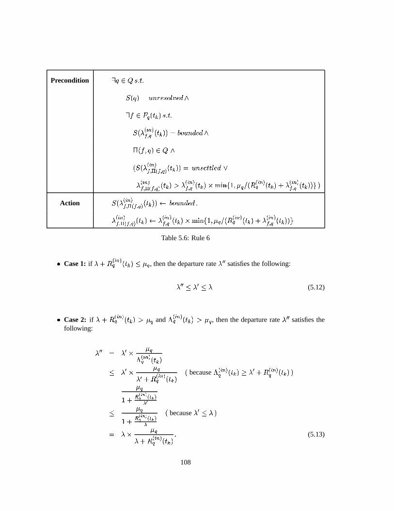
Precondition� � � � � � � �
� � � � � � � 8 � � � � 8 � �� � ��� � ���4� � � � �� � ���
����! � ���4� � � ��� � � 8 � �
( � � � � � � �� � � � �
����! � � � � ��� � � � � � 8!�4� � 8 � �
���� ��! � � � � ��� � ������
� ��! � ��� � ������� � ��� � � � � � �
� �� ��� � � ���
����! � ���4� �
Action � � � �� �� � �! � � ���4� � � ��� � � 8 � �
�"����� � � � � ��� � � �"�
���� � ���4� ����� � � ��� � � � � � �
���� ���4� �� �"�
� �� � ��� � �
Table 5.6: Rule 6
� Case 1: if � � � ����� ���4� � � � , then the departure rate � satisfies the following:
� � � � � (5.12)
� Case 2: if �%� � �� �� ��� � � � � and 1 �
� �� ��� � � � � , then the departure rate � satisfies the
following:
� � � � � �1 �� �� ��� �
� � � � �� � � �
���� ���4� � because 1 �
���� ���4� � � � � �
� �� ���4�
� � �� �
�������0 � %��6����
� � �� �
� �����0 � %��6��
� because � � �
� � � � �� � � �
���� ��� � � (5.13)
108

� Case 3: if �%� � �� �� ��� � � � � and 1 �
� �� ��� � � � � , then the departure rate � satisfies the
following:
� � � � � � � � �
���� ���4�
� � � � � ����� ���4� � � �
� �� �� ��� � �� � � because � � � �
� �� ��� � �� � �
� � � � �� � � �
���� ��� � � (5.14)
Combining all three cases, we prove the lemma. �Lemma 6 informs us how to compute the upper bound on the departure rate for an input flow
variable in the bounded state. If the flow does not disappear into a sink, we can use this upper boundon the departure rate to bound the corresponding input flow variable at its next output port.
Note that the ultimate objective of the algorithm is, actually, to resolve every output port in thetopology under consideration. Rule 1 has the highest priority because every time it is applied, anew output port is resolved and some flow variables in
� may be settled. Although Rule 2 does not
resolve a port, it identifies a transparent port and propagates its settled flow rates downstream, whichpossibly leads to new ports found applicable to Rule 1. Rule 3 neither resolves a port nor identifiesa transparent port, but it propagates already-settled flow rates through a transparent port. The next3 rules establish upper bounds on flow variables. Because the first 3 rules have higher priority, flowvariables tend to be settled before the last 3 rules are applied. Once no port is applicable to the first3 rules, we try the last 3 rules, in the hope of identifying more transparent ports with tighter upperbounds.
Let �
denote Rule � , where
� � � � �. In the implementation, for each rule �
, we maintain
a list of ports, denoted by� � � . The ports on list
� � � must satisfy the precondition to rule �
. After
the time step setup, we check all the ports that have input flows: if a port � is the ingress port ofall the flows that traverse it, it is added onto list
� � . We then iterate over the ports on the 6 lists.Each time, we grab an arbitrary port � from the list with the highest priority and process it as thecorresponding rule, say rule � , indicates. After the port is processed, we remove it from list
� � .Because we update the states of the input flow variables at downstream ports, some of them maysatisfy the precondition to a rule. If we find such a port, we put it onto the corresponding port list ifit is not there yet. The above iteration terminates when all the 6 port lists are empty. At this time,Phase I finishes.
In order to check whether a port satisfies the precondition to a rule in constant time, we need tobe careful in the implementation. Some auxiliary variables are introduced for this purpose. At eachport, we keep both the number of input flow variables in the settled state and the number of inputflow variables in the bounded state. After updating the state of one or more input flow variables ata port, we update these two variables correspondingly. We can then compare the number of settledinput flow variables and the total number of input flow variables at this port and decide whetherRule 1 is applicable. If Rule 1 cannot be applied, we can check whether all the input flow variablesare in either settled or bounded state and then determine whether Rule 2 is applicable. With aid of
109

the two auxiliary variables, we can check whether a port satisfies the precondition to Rule 1 or Rule2 in constant time.
Note that for each of the last four rules, its precondition requires that at least one input flowvariable satisfy certain conditions. Hence, for each of these rules, we use a list to keep all the inputflow variables that satisfy these conditions. After we process a port and update the state of an inputflow variable at the corresponding downstream port, we check whether that flow variable satisfiesthe conditions in the precondition to any of the last four rules. If so, we put the flow variable ontothe corresponding list. When a port that satisfies one of these rules is processed, we choose anarbitrary flow variable from the corresponding list, remove it from there, and process it as the rule’saction indicates. In this way, it is unnecessary to traverse the states of all the input flow variablesand check whether there exists an input flow variable that satisfies certain conditions.
In order to apply Rule 5 or 6, we need to know the sum of all the input flow rates that are settledso far. We introduce another variable to keep this value at each port. Once an input flow variable issettled, we add the settled input rate onto this variable. Hence, we need only constant time to obtainthe sum of all the input flow rates that are settled.
From the above discussion, we have the following property:
Lemma 7 After a port is processed, if there exists at least one unprocessed port in Phase I, we needonly constant time to decide which port can be processed next.
The following lemma tells us the possible states which a flow variable may have after Phase I.
Lemma 8 After Phase I, every flow variable must be in the settled or bounded state.
Proof: We prove it by contradiction. Suppose that flow variable � is in the unsettled state afterPhase I. We search the first flow variable that is not in the unsettled state along the upstream di-rection on the flow’s path. There must exist such a flow variable because at least the flow variablecorresponding to the ingress rate of the flow is in the settled state. Let �� be this flow variable. Sup-pose that � belongs to port � , and the next port on the flow’s path is � . If port � is in the resolvedstate, then the corresponding flow variable at port � must be settled from Rule 1; if port � is in thetransparent state, then either Rule 3 or Rule 4 can be applied on flow variable � ; if port � is in theunresolved state, then either Rule 5 or Rule 6 can be applied on flow variable �� . In either case, acontradiction follows. �
We use the example network in Figure 5.5 to illustrate the application of the 6 rules. Given thetwo configurations shown in Table 5.7, our algorithm works as follows in Phase I:
� Configuration 1: Table 5.8 presents how the rule-based flow update computation processworks on this configuration. Step 1 applies Rule 1 to resolve port � � . Step 2 applies Rule 5 tocompute the upper bound on � �
� �� � � . Because � �
���� � � � � �
� �� � � � � � , port � � can be identified
as transparent; hence, the settled arrival rate of flow � � into port � � can be propagated throughit and then used to settle � �
� �� � � . Thereafter, Rule 1 can be used to resolve ports � � , � � , � � , � � ,� � , and � � successively.
110

Configuration 1 Configuration 2
� �� �� � � � � � �
� �� � � � � � � � �
� �� � � � � � �
���� � � � � � �
� �� ����6 � � � � �
� �� � � � � � � � � �
� ����6 � � � � �
���� � � � � � � �
� �� �� � � � � � �
� �� � � � � � � �
� �� � � � � � �
���� � � � � �
� �� ���� � � � � �
� �� � � � � � � � �
� ���� � � � � �
���� � � � � � �
���� ���� � � � �"�
� ����� � � � � � � �"�
� ���� � � � ���
������ � � � � � �
���� ����6 � � � �"�
� �� � � � � �"�
� ����6 � � � ���
���� � � � �
� �� ���� � � � � �
� ����� � � � � � � � �
� ���� � � � � �
������ � � � � � �
���� �� � � � � �"�
� ��� � � � � � � �"�
� �� � � � � ���
����� � � � � � �
Table 5.7: Two Configurations
� Configuration 2: Table 5.9 presents how the rule-based flow update computation processworks on this configuration. Step 1 applies Rule 1 to resolve port � � . Step 2 applies Rule5 to compute the upper bound on � �
���� � � . Because � �
���� � � � � �
� �� � � � � � , port � � cannot be
identified as transparent as on the previous configuration. Step 3 applies Rule 5 to computethe upper bound on � �
� �� � � ; Step 4 applies Rule 5 to compute the upper bound on � �
� ���� � � ; Step 5
applies Rule 5 to compute the upper bound on � ����� �6 � . In step 6, because � �
���� � � �"�
���� � � � � � ,
port � � is identified as transparent. Step 7 uses Rule 4 to compute the upper bound on � �� ����� � � .
The final step applies Rule 5 to compute the upper bound on � �������6 � � and � �
� ���� � � .
Both Tables 5.8 and 5.9 provide only a sample execution path for each configuration becauseafter some steps there exist multiple choices on which ports should be processed. With configura-tion 1, all ports in the topology are resolved after Phase I; it is evident that with aid of transparencyof port � � , the circular dependence among flow variables in the network can be entirely removed.When this occurs, the algorithm stops after Phase I. With configuration 2, however, all ports but port� � are still unresolved; although port � � is also identified as transparent, it does not help reduce thewhole circular dependence. When there still exist some unresolved ports, the algorithm proceedsinto Phase II.
Phase II: Dependence Graph Generation. Owing to circular dependence, some output portsstill remain unresolved after Phase I. As discussed in Section 5.4.3, the fixed point algorithm stands
111

Step Rule Processing
1 1 � � � � � � 8 � � � ��8 � � � � �"�� �� � � � � � 8!�4� �98 � � � � �"�
� �� � � � 8!�4� �98 �
2 5 � � � ����� � � � � ��� � � 8 � � � �
���� � � � � �
���� � � �
3 2 � � � � � � � � � � � ��� 8 �"� � � � �"����� � � � � 8!�4� �98 � � �"�
���� � � � ���
� �� �
4 1 � � � � � � 8 � � � ��8 � � � � �"�� ���� � � � � 8!�4� �98 � �
� ������� � � � � �
� ���� � � ������� � ��� � � � �/1 �
� �� �
5 1 � � � � � � 8 � � � ��8 � � � � � �� �� � � � � 8!�4� �98 � �
� �������6 � � � �
� ����6 � � ������� � ��� � � � �/1 �
� �� �
6 1 � � � � � � 8 � � � ��8 � � � � � �� ����6 � � � � 8!�4� �98 � �
���������6 � � � �"�
� ����6 � ������� � ��� � � �/1 �
� ��
7 1 � � � � � � 8 � � � ��8 � � � � �"�� ����6 � � � � 8!�4� �98 � �
� �������6 � � � � �
� ����6 � � ������� � ��� � � � �/1 �
� �� �
� � �"����� � � � � � 8 �$� �98 � � ���
� �� � � � � �"�
� �� � � � ������� � ��� � � � �/1 �
� �� �
8 1 � � � � � � 8 � � � ��8 � � � � � �� �� � � � � 8!�4� �98 � �
� ����� � � � � �
� �� � � � ������� � ��� � � � �/1 �
� �� �
Table 5.8: Flow Update Computation for the Network in Figure 5.5 (Configuration 1)
112

Step Rule Processing
1 1 � � � � � � 8 � � � � 8 � � � � � �� ���� � � � � 8 �$� �98 � � � � � �
� �� � � � 8!�4� � 8 �
2 5 � � � �� �� � � � � ��� � � 8 � � � �
� �� � � � � �
� �� � � �
3 5 � � �"�� �� � � � � ��� � � 8 � � �"�
� �� � � � �"�
� �� �
4 5 � � � �� ���� � � � � ��� � � 8 � � � �
� ���� � � � � �
� ���� � �
5 5 � � �"�� ����6 � � � ��� � � 8 � � �"�
� ����6 � � �"�
� ����� � �
6 2 � � � � � � � � � � � � � 8 �"�7 4 � � � �
� �� � � � � � ��� � � 8 � � � �
� �� � � � � � �
� �� � �
8 5 � � � �� ����6 � � � � ��� � � 8 � � � �
� ����6 � � � � �
� ����� � �
� � �"�� ���� � � � � ��� � � 8 � � �"�
� ���� � � � �"�
� ���� � �
Table 5.9: Flow Update Computation for the Network in Figure 5.5 (Configuration 2)
113

out as the only practical solution to determining the rates of those unsettled flow variables in� .
In order to reduce the computation cost on fixed point iterations, we try to minimize the number offlow variables that are involved. The example network with the second configuration is used to buildsome intuition on which flow variables should be considered. After Phase I, we still do not know theexact rates of flow variables � �
���� � � , � �
� �� � � , � �
� ���� � � , � �
� ����6 � , � �
� ����6 � � , � �
� ���� � � , and � �
������� � � . Remember that
port � � has been identified as transparent, which suggests that � �� �� � � must be equal to � �
���� � � � . On the
other hand, � �� ����6 � � actually does not stay in any cycle: settling it entirely depends on the resolution
of port � � . These two observations lead to the following optimizations:
� Optimization 1: We exclude every flow variable associated with a transparent port from thefixed point iterations;
� Optimization 2: We exclude every flow variable that is not on any circular dependency fromthe fixed point iterations;
Now we discuss how to implement these two optimizations by constructing dependence graph�
. First we construct set�
, which contains all the output ports in the unresolved state:
� � �&� �4� � � � � � � � � � � 8 � � � ��8 � � (5.15)
Note that some output ports whose states are transparent may still have some unsettled inputflow variables, but they are excluded from set
�based on the first optimization. The ports in
�
form the vertices in dependence graph�
. We use
to denote the set of edges in graph�
. This setis initialized to be empty. Every edge 8 is associated with a set of flow variables, denoted by ��� �98 .For every port � in
�, we process each of its input flow variables as follows: search the first output
port � downstream on the flow’s path that is also included in set�
; if such a port can be found, adirected edge from port � to port � , denoted by 8 � � � � , is added to
(if it is not in
yet) and the
corresponding input flow variable at the receiving port is added into set ��� �98 � � � � . After all portsin
�have been processed, the resulting graph
�has the following property: no port in graph
�has
indegree 0. If there exists a port with indegree 0, then its resolution does not depend on any otherport’s state, and therefore, it must have already been resolved in Phase I, which contradicts it beingin set
�.
However, it is likely that some ports in�
have outdegree 0. This happens when input flowvariables associated with these ports are not in any circular dependence. In the example network,port � � has outdegree 0 because flow variable � �
������ � � is not in the circular dependence formed by
other variables. According to the second optimization, we remove the ports with outdegree 0 fromgraph
�and all the edges that point to them. After removing a port with outdegree 0, we decrease
the outdegrees of those ports that have an edge pointing to it by 1; if the outdegree of a port becomes0 thereby, it should also be removed from graph
�. Then the above process repeats, until no port
with outdegree 0 exists in dependence graph�
. Phase II finishes when the process terminates. Notethat when we prune the ports with outdegree 0 from the graph, no port with indegree 0 should beintroduced. Hence, the following lemma should hold after Phase II:
114

Lemma 9 In the final graph�
, no port has indegree 0 or outdegree 0.
As for the example network with the second configuration, the final dependence graph�
isshown in Figure 5.6.
q0
q q1 2
λf q,5 0
λf q,0 1
λf q,1 2
λf q, 32
3q
q5
(in)
(in)(in)
(in)
λf3 q 5,(in)
Figure 5.6: Dependence Graph for the Example Network with Configuration 2
Phase III: Fixed Point Iterations and Residual Flow Update Computation. The fixed pointalgorithm described before operates on all the input flow variables in the network except thosethat correspond to the ingress rates of flows. Our approach aims to minimize the number of flowvariables involved in the fixed point iterations. We construct another vector
� �to contain all the
flow variables that need to be settled by the fixed point algorithm. For every edge 8 in dependencegraph
�(i.e., 8�� ), we put all the flow variables in � � �98 into
� �. Using Equation (5.3), we
can form a set of equations of variables in� �
. The fixed point algorithm is then applied to find theroot of this group of equations. As discussed in Section (5.4.3), the algorithm starts from an initialestimate on
� �. The simplest estimate is
�, in which all the variables in
� �are 0. This estimate may
be very far from the real fixed point; a lot of iterations are, therefore, necessary before that fixedpoint is approached. Hence, our solution adopts an alternative estimate: since every flow variablein
� �must have an upper bound when Phase I finishes, these upper bounds on the variables in
� �form the initial estimate. Therefore, tighter upper bounds on flow variables found in Phase I mayhelp reduce the number of iterations required in the fixed point algorithm.
The fixed point iterations terminate when the maximum relative difference between successive
estimates on any flow variable in� �
is less than a tolerance � . We use� � � � � � � , � � �� ��� ���� � �
and��� � � � � � � to denote the estimate on the
�-th variable in
� �after iteration � . Then, the termination
criterion is
� ������ � ������ �
� � � �5 � � � � � � � � �
5 � � � � � �
� � � � � � � �
��
(5.16)
Once the fixed point algorithm terminates, we change the state of each flow variable in� �
to settled.
115

In the example,� �
is constructed as
� �"�� �� � � � �"�
� �� � � � ���
������ � � � �"�
���� �6 � � � �"�
� ���� � � � �
(5.17)
Using Equation (5.3), we form a group of equations as follows:
���������������� ���������������
���� �� � � � �"�
� �� � � � � min � ��� � � � � � �"�
� �� � � � � �"�
������ � � �
� �� �� � � � � �
� �� � � min � ��� � � � � � �
� �� � � � �
���� � � �
� �� �� � � � � � �
� �� � � � � min � ��� � � � � � � �
� �� � � � � � �
���� � �
� �� ����6 � � � � �
� ���� � � � min � ��� � � � � � � �
� ����6 � � � � �
������ � � �
� �� ���� � � � � �
� ����� � � � min � ��� � � � � � � �
� ���� � � � � �
���� �6 � � �
(5.18)
The fixed point algorithm is then applied to solve Equation (5.18), starting from an initial estimatein which every flow variable in
� �uses its upper bound obtained in Phase I. Recall that in Phase II,
transparent ports and ports with outdegree 0 are excluded from�
. At these ports, therefore, someinput flow variables are still unsettled after the fixed point iterations. We can resume the rule-basedflow update computation and resolve all the unresolved ports. In the example, � �
� �� � � � and �"�
���� � � are
not settled after the fixed point iterations. Because both input flow variables at port � � are settled,Rule 1 can be used to compute ���
������ � ; �"�
� ����6 � � can also be calculated by applying Rule 1 on port ��� .
After Phase III, all output ports in the network have been resolved. The algorithm then endshere. In the following sections, we will discuss the issues regarding the convergence behavior,performance, and accuracy of our algorithm.
5.5.2 Convergence Behavior
If the flows in the network form circular dependencies that cannot be resolved in Phase I, the fixedpoint algorithm is necessary to settle the unsettled flow variables associated with these circulardependencies. As mentioned in Section 5.4.3, the convergence behavior of the fixed point iterationsdirectly affects the performance of our algorithm. For example, if the fixed point iterations diverge,then our algorithm may never terminate and its foundation is thus severely undermined.
In mathematics, two fixed point theorems are often used to prove the existence of fixed points[30]. The Brouwer fixed point theorem states that every continuous function from a nonempty,compact and convex subset of � � to itself must have at least one fixed point. Although elegant,the Brouwer fixed point theorem is non-constructive: it does not describe how to find the fixedpoints. Rather, the Banach fixed point theorem provides an approach to discovering fixed pointsfor functions that are contraction mappings. A function � � � � � is said to be a contractionmapping if there exists a constant � with
� � � �such that
� � � ��� � � ��� � � � � ��� � � (5.19)
116

where the real valued function� � � � � � � is a distance function or metric. The Banach
fixed point theorem states that every contraction mapping has a unique fixed point. For an arbitrary� � � � � � , iterate as � � � 5 � � � � ��� � � � . The sequence converges to the unique fixed point. Hence,the Banach fixed point theorem provides a constructive approach to finding the fixed point. Inorder to use the Banach fixed point theorem to guarantee convergence of our algorithm, we needto prove that function
�in Equation (5.10) is a contraction mapping. As discussed in Section
5.4.3, however,� � � is a multi-dimension nonlinear system of equations containing
� � � functions,whose mathematical analysis is well known to be difficult, especially when there are a large numberof variables in the system.
In [62], a related problem has been investigated in the context of multi-class networks with FIFOservice disciplines. The main theorem in it establishes the existence of a unique fixed point solutionfor a reentrant line that traverses multiple stations whose service rates are independent of the line’sstage. A reentrant line and a station resemble a flow and a port in our problem respectively. In thefinal remark of the paper, it is also claimed that the theorem can be extended for the cases in whichmultiple reentrant lines exist.
The theoretical results in [62] may be helpful in establishing the existence of a unique solutionto our problem. Even so, however, we are still unclear of whether the fixed point iterations finallyconverge to that fixed point. Furthermore, even if they converge, how fast they converge still remainas a mystery to us; a slowly convergent algorithm may lead to poor performance because a lotof computation work is spent on the iterations before a fixed point is reached. Provided thesechallenges on understanding the convergence behavior of our algorithm, we put an upper bound onhow many iterations are allowed in a time step. In a real network, traffic traversing across a linksuffers some delay. We assume that all the edges in the dependence graph built in Phase II areassociated with a universal delay
�. Then, iterations in the fixed point algorithm can be considered
as periodically updating the states of flow variables every�
simulation time units. Recall that thetime step size is � simulation time units. Therefore, there are at most � �%� � � iterations permissiblewithin one time step, where � � � is the largest number no greater than � . The selection on
�in our
approach is given as follows. Let� � �98 denote the aggregate delay from the node where edge 8
starts to the node where edge 8 ends on flow’s � ’s path in the real network. For each edge 8 in
,we associate with it the largest aggregate delay that any flow across it suffers. Then among all theedges in the dependence graph, we pick the one that has the largest aggregate delay. We choose
�
as follows:� � � ���
�
- � ����/-�.�� � �"� � � �98 � (5.20)
The above upper bound is aimed at avoiding excessive number of iterations that the fixed pointalgorithm has to take before the fixed point is found or when the fixed point cannot be found throughiterations. In all the following experiments, we actually find that the fixed point algorithm convergeswithin a small number of iterations, and the upper bounds have never been reached.
In Table 5.10, we summarize four real topologies that are used in the simulation experimentsin this section and the following sections. Top-1, which is illustrated in Figure 4.7, is a POP-levelATT USA backbone network. A flow is created between any pair of POPs, which thus leads to702 flows in total. The bandwidth of each link is set to be 100Mbps. This topology later will
117

Topology # nodes # directional links # flows Link bandwidth
Top-1 27 88 702 100 Mbps
Top-2 244 1080 12200 2488 Mbps
Top-3 610 3012 61000 2488 Mbps
Top-4 1126 6238 168900 2488 Mbps
Table 5.10: 4 Topologies Used in the Simulations
be used in Section 5.5.3 to do performance comparison between the time-stepped coarse-grainedtraffic simulator and the packet-oriented simulator; a comparatively low link bandwidth enables usto finish a certain number of simulation runs with the packet-oriented simulator in a reasonableperiod of time. The other three topologies are obtained from the Rocketfuel project1 . Top-2 isthe router-level Exodus backbone; Top-3 consists of two router-level ISP backbones, the Exodusbackbone and the Above.Net backbone, which are connected through some peering links; Top-4further augments Top-3 by adding another router-level ISP backbone, Sprint backbone, to it. InTop-2, Top-3, and Top-4, every router picks 50 routers from its own backbone and directs a flow toeach of them; it also picks 50 routers from each other backbone in the topology and directs a flowto every one of them. Hence we get the total numbers of flows shown in the table. We use the PPBPtraffic model to generate the ingress rate for each flow. The Hurst parameter is 0.8. The coefficientof variance (COV), which is the ratio of the standard deviation to the mean, is a common measureof traffic burstiness [74]. In our experiments, we test two COVs, 5 and 0.5. The tolerance � , whichis used to determine whether fixed point iterations should be terminated (See Equation (5.16)), is0.001.
In the experiments studying the convergence of our algorithm, we simulate Top-2, Top-3, andTop-4 for 200 time steps, each spanning 5 seconds. Figures 5.7 - 5.11 give the histogram of thenumber of ports on the dependence graph in Phase III of a time step, and the number of iterationsused to reach fixed point solutions, on single runs of 200 time steps with 2 COVs. The simulationresults can be analyzed from the following aspects:
� The same COV, the same link utilization, different topology sizes. Under this setting, weconsider how the topology size affects the convergence behavior. When the simulated topol-ogy contains more nodes and thus more flows, more ports may appear on the dependencegraph in Phase III. Although the traffic load at each port is maintained at the same level, suchgrowth is observed to be sup-linear with the topology size, measured by the number of nodes.For example, consider the results when the link utilization is 50% and the COV is 5. The
1http://www.cs.washington.edu/research/networking/rocketfuel/
118

0
20
40
60
80
100
120
140
160
180
200
0 2 4 6 8 10 12 14
Num
ber
of ti
me
step
s
Number of ports
0
20
40
60
80
100
120
140
160
180
200
0 0.5 1 1.5 2 2.5 3 3.5 4N
umbe
r of
tim
e st
eps
Number of iterations
COV = 5
0
0.5
1
1.5
2
2.5
3
3.5
4
0 0.5 1 1.5 2 2.5 3 3.5 4
Num
ber
of ti
me
step
s
Number of ports
0
20
40
60
80
100
120
140
0 0.5 1 1.5 2
Num
ber
of ti
me
step
s
Number of iterations
COV = 0.5
Figure 5.7: Histogram of Ports on Circular Dependencies, and Iterations per Time-step, for Top-220% Link Utilization
119

0
5
10
15
20
25
30
0 5 10 15 20 25 30 35 40
Num
ber
of ti
me
step
s
Number of ports
0
10
20
30
40
50
60
70
0 1 2 3 4 5 6 7
Num
ber
of ti
me
step
s
Number of iterations
COV = 5
0
10
20
30
40
50
60
0 5 10 15 20 25 30 35 40 45
Num
ber
of ti
me
step
s
Number of ports
0
20
40
60
80
100
120
140
0 1 2 3 4 5 6 7
Num
ber
of ti
me
step
s
Number of iterations
COV = 0.5
Figure 5.8: Histogram of Ports on Circular Dependencies, and Iterations per Time-step, for Top-250% Link Utilization
120

0
5
10
15
20
25
30
35
40
45
0 2 4 6 8 10 12 14
Num
ber
of ti
me
step
s
Number of ports
5
10
15
20
25
30
35
40
45
50
0 1 2 3 4 5 6 7N
umbe
r of
tim
e st
eps
Number of iterations
COV = 5
0
5
10
15
20
25
30
35
40
45
50
0 1 2 3 4 5 6 7 8
Num
ber
of ti
me
step
s
Number of ports
0
1
2
3
4
5
6
7
8
0 0.5 1 1.5 2 2.5 3 3.5 4
Num
ber
of ti
me
step
s
Number of iterations
COV = 0.5
Figure 5.9: Histogram of Ports on Circular Dependencies, and Iterations per Time-Step, for Top-320% Link Utilization
121

0
2
4
6
8
10
12
14
16
18
0 10 20 30 40 50 60
Num
ber
of ti
me
step
s
Number of ports
0
10
20
30
40
50
60
70
80
90
0 2 4 6 8 10
Num
ber
of ti
me
step
s
Number of iterations
COV = 5
0
10
20
30
40
50
60
70
80
0 10 20 30 40 50 60
Num
ber
of ti
me
step
s
Number of ports
0
5
10
15
20
25
30
35
40
45
50
0 1 2 3 4 5 6 7 8
Num
ber
of ti
me
step
s
Number of iterations
COV = 0.5
Figure 5.10: Histogram of Ports on Circular Dependencies, and Iterations per Time-Step, for Top-350% Link Utilization
122

0
2
4
6
8
10
12
0 10 20 30 40 50 60 70 80
Num
ber
of ti
me
step
s
Number of ports
0
20
40
60
80
100
120
140
0 2 4 6 8 10N
umbe
r of
tim
e st
eps
Number of iterations
Top-4 Backbone 20% Link Utilization
0
2
4
6
8
10
12
14
0 20 40 60 80 100 120 140 160
Num
ber
of ti
me
step
s
Number of ports
0
20
40
60
80
100
120
140
0 2 4 6 8 10 12
Num
ber
of ti
me
step
s
Number of iterations
Top-4 Backbone 50% Link Utilization
Figure 5.11: Histogram of Ports on Circular Dependencies, and Iterations per Time-Step, for Top-4(COV = 5)
123

average number of ports on the dependence graph in Phase III is 14 for Top-2, 39 for Top-3,and 128 for Top-4, but the sizes of Top-3 and Top-4 are 2.5 and 4.6 times as that of Top-2respectively. This can be explained as follows. As the topology size increases, although theaverage link utilization is maintained at the same level, congested ports are more likely to bedependent on each other because on average more flows traverse a port. Another observationfrom the simulation results is that as the topology size increases, the average number of iter-ations required to reach a fixed point increases slightly; this is reasonable because more portsare on the dependence graph in Phase III.
� The same COV, the same topology, different link utilizations. The impact that the trafficload in the network has on the convergence behavior of our algorithm is clear: if the averagelink utilization is higher , then it is more likely for a port to be congested and thus moreports appear on the dependence graph in Phase III. This is also observed from the simulationresults. For example, consider the results when the COV is 5. If the link utilization is 20%,the average number of ports on the dependence graph in Phase III corresponding to Top-2,Top-3, and Top-4 is 0, 5, and 55 respectively, but if the link utilization is 50%, the averagenumber of ports on the dependence graph in Phase III corresponding to Top-2, Top-3, andTop-4 is 14, 39, and 128 respectively.
� The same topology, the same link utilization, different COVs. The COV is a metric oftraffic burstiness. Its impacts on the convergence behavior of our algorithm vary with thetraffic load in the topology. When the link utilization is 20%, if the COV is higher, moreports appear on the dependence graph in Phase III; when the link utilization is 50%, if theCOV is higher, it seems that fewer ports appear on the dependence graph in Phase III. Thisobservation can be explained as follows. When the link utilization is low, the traffic needsto be highly bursty to cause congestion in the network. When the link utilization is high, acertain level of burstiness is enough to cause congestion. However, if the mean is the sameand the COV is relatively large, then the bursty traffic pattern generated at the ingress nodeof a flow has high peak rates, followed by long “silent” periods (i.e., the flow has rate 0).The peak rates, if exceeding the link bandwidth associated with the ingress port, are reduced,causing the ports on the flow’s path to see less traffic. Therefore, when the link utilization andthe COV are both high, it is observed that fewer ports appear on dependence graph in PhaseIII from the simulation results. Another observation is that when the COV is higher and thetraffic is thus more bursty, the number of ports that appear on the dependence graph in PhaseIII over the 200 time steps vary in a larger range. This is because if the traffic is less bursty,the change on the aggregate arrival rate into a port is less dynamic across the time steps andcongestion occurs more regularly in the network.
In summary, our algorithm is able to significantly reduce the number of ports in the fixed pointiterations. Under any traffic load and any COV, the largest proportion of ports that appear on thedependence graph in Phase III is 4.4%, 2.8%, and 3.4% for TOP-2, TOP-3, and TOP-4 respectively.Furthermore, the fixed point solution in our algorithm can converge within a small number of iter-ations. In all the experiments, we have observed that at most 12 iterations are necessary to reach asolution that satisfies the termination criterion (5.16).
124

5.5.3 Performance
In Section 5.4, we have discussed the performance of some specific solutions in diverse settings.Corollaries 3 and 4 tell us that the fixed point algorithm does not provide the optimal performanceif it is applied on some specific networks like feed-forward networks or ones that have sufficientbandwidth. Then how does our algorithm perform on these networks? Following the same notationsthere, we use � and � to denote the total number of flows in the network and the average numberof output ports on a flow’s path. The following theorem establishes the time complexity of ouralgorithm when applied on a feed-forward network.
Theorem 5 Given a feed-forward network, the time complexity of the algorithm described in Sec-tion 5.5.1 is � � � � � .
Proof: There is no circular dependence among flow variables in a feed-forward network. Hence,all ports are resolved in Phase I. In our implementation, Rule 1 is iteratively used to resolve all theoutput ports in a feed-forward network because it has the highest priority. The state of every outputport in the topology is read or updated for a constant number of times when it is resolved with Rule1; correspondingly, every input flow variable is also read or updated for a constant number of timesin the course of the computation. Lemma 7 tells us that after a port is processed, only constanttime is needed to find the next unprocessed port. Therefore, the time complexity of the algorithm is
� � � � � . �The next theorem establishes the time complexity of our algorithm when it is applied on a
network with sufficient bandwidth.
Theorem 6 Given a network with sufficient bandwidth, the time complexity of the algorithm de-scribed in Section 5.5.1 is � � � � � .
Proof: When our algorithm is used to resolve the ports in a network with sufficient bandwidth, allthe flow variables are settled in Phase I because transparency can make the ingress rate of everyflow be propagated to its destination. Only the first three rules are applied because they have thehigher priorities than the other three. The state of each input flow variable changes exactly oncefrom unsettled to settled. Since there are � � � � � input flow variables, the total computation coston updating the states of the input flow variables is � � � � � . On the other hand, whenever a ruleis applied on a port, we propagate the settled rate of at least one input flow through it and settlethe corresponding input flow variable at the next hop. The total computation cost on reading orupdating the states of the ports is thus ��� � � � . Therefore, the time complexity of the algorithmis thus � � � � � . �
Theorems 5 and 6 tell us that on some specific networks, our algorithm requires less asymptoticcomputation cost than the original fixed point algorithm. It actually has the same asymptotic timecomplexity as the particular solutions discussed in Sections 5.4.1 and 5.4.2. However, our algorithm,like the original fixed point algorithm, has the power to solve the problem on networks involvingcircular dependencies.
125

If circular dependencies cannot be completely removed from the topology after Phase I, ana-lyzing the time complexity of our algorithm becomes more complicated for two reasons. First, it isdifficult to establish exactly how many times the upper bound of a flow variable is updated in PhaseI. Our strategy is to lower the upper bound of every flow variable as much as we can, in the hope thatmore transparent ports can thus be exposed in Phase I; in addition, a tighter upper bound on a flowvariable will provide a better initial estimate on it later for the fixed point algorithm. This strategy,however, makes it difficult to establish how many times the upper bound of a flow variable has beenchanged, especially in a large topology where many ports are in circular dependence. On the otherhand, the performance of our algorithm is also contingent on how many ports remain unresolvedafter Phase I and how many iterations have been done in the fixed point algorithm. Both factorsare topology-dependent, and the latter also depends on the precision tolerance � in the terminationcriterion (5.16).
We therefore empirically investigate the performance of our algorithm under realistic topologies.The four topologies in Table 5.10 are simulated at two traffic intensity levels: 20% average linkutilization and 50% average link utilization. The time step we choose is 5 seconds, which is muchlarger than the typical end-to-end delays even in a large network. We use the PPBP traffic modelto generate the ingress rate for each flow. The Hurst parameter is 0.8. As we said in Section 5.5.2,traffic burstiness can be measured with COV. In our experiments, we test two COVs, 5 and 0.5. Allthe experiments are done on a 1.5GHz PC with 2Gb of memory. The average execution times pertime-step for these four topologies under different traffic loads are presented in Table 5.11. Becausethe variations on these execution times are all quite small, we do not show the confidence interval inthe table. We do not have the results for Top-4 when the COV is 0.5 because the memory requiredin the simulation exceeds the physical limit.
All the simulations are completed within less than 5 seconds, the time step we choose. It sug-gests that these simulations are finished in real time. From the results shown in Table 5.11, it seemsthat if the traffic is more bursty, less simulation execution time is required. This is counter-intuitivebecause high variation usually cause more congestion, thus putting more ports on the dependencegraph in Phase III. We explain this observation as follows. When the COV is large, traffic generatedfrom the PPBP model is actually very bursty. As said in Section 5.5.2, if the COV is larger, the peakrates in the bursts are higher, followed by longer “silent” periods. In our implementation, when aflow does not have traffic to emit at a time step, we do not push rate 0 along its path because it doesnot affect the computation of flow variables. Obviously, if more flows have ingress rate 0 at a timestep, there are fewer flow variables that need to be settled. In addition, from the simulation resultsshown in Section 5.5.2, we know that when the link utilization is high, higher burstiness actuallyreduces the number of ports on the dependence graph in Phase III. These two observations bothexplain why simulations configured with higher COVs take less time to finish.
We have also done some experiments on Top-1 to obtain the relatively execution speedup of thetime-stepped coarse-grained traffic simulator against a pure packet-level network simulator. TheHurst parameter is 0.8. We test two COVs: 5 and 0.5. We also vary the ingress rates of flowsto obtain different average link utilizations in the network. The relative execution speedups, as afunction of average link utilization, are presented in Figure 5.12. It is clear that time-stepped coarse-grained traffic simulation has achieved execution speedups at several orders of magnitude under
126

COV = 5 COV = 0.5
Topology secs/round secs/round secs/round secs/round
(20% link util) (50% link util) (20% link util) (50% link util)
Top-1 0.0026 0.0026 0.0051 0.0052
Top-2 0.051 0.051 0.1988 0.2380
Top-3 0.283 0.285 1.4895 1.8740
Top-4 0.852 0.907 - -
Table 5.11: Average Execution Time per Time-Step
both traffic loads. We have also observed that with increasing average link utilization, the speedupover the pure packet-level simulator also improves. This is because the performance of a packet-level traffic simulator is directly affected by the amount of traffic traversing through the network,but performance of the time-stepped coarse-grained traffic simulator is relatively insensitive to theabsolute traffic load in the network.
From Figure 5.12, we have noticed that the relative speedup curve grows sublinearly as theaverage link utilization exceeds 50%. There are two reasons for this. First, when the traffic loadincreases up to a high level, the pure packet-level traffic simulator drops a portion of traffic owingto congestion. Second, heavy traffic load causes more output ports to become circularly dependentand the fixed point algorithm thus has to operate on more unsettled flow variables in Phase III.
In addition, comparing the two curves with different COVs, we can find that a larger COV leadsto less relative speedup from the time-stepped coarse-grained traffic simulator. When a pure packet-level simulator is used, if the traffic is more bursty, more packets are dropped in the network, whichsignificantly reduces the execution time. Although from Table 5.11 we know that with a largerCOV, the time-stepped coarse-grained simulation also needs less execution time, it has a smallerimpact on the speedup than the reduced execution time due to packet losses by the pure packet-levelsimulator.
5.5.4 Accuracy
In this section, we discuss the accuracy of our approach as a background traffic generator againstthe pure packet-oriented approach. We modify topology Top-1 by attaching an end host to eachPOP node in it. The background traffic is simulated with two different techniques: our time-steppedcoarse-grained simulation and conventional packet-level simulation. We vary the average back-
127

500
1000
1500
2000
2500
3000
3500
10 20 30 40 50 60 70 80
Spee
dup
over
pac
ket s
imul
atio
n
Background traffic load (%)
COV = 5COV = 0.5
Figure 5.12: Speedup of Time-Stepped Coarse-Grained Traffic Simulator over Packet-OrientedSimulator (Top-1)
1.5e+06
2e+06
2.5e+06
3e+06
3.5e+06
4e+06
4.5e+06
5e+06
0 0.1 0.2 0.3 0.4 0.5 0.6 0.7 0.8 0.9
TCP goodput (bytes/sec)
Background traffic load
coarse flowspacket flows
Figure 5.13: TCP Goodput (95% Confidence Interval)
128

0.7
0.75
0.8
0.85
0.9
0.95
1
0 0.1 0.2 0.3 0.4 0.5 0.6 0.7 0.8 0.9
Delivered fraction of UDP traffic
Background traffic load
coarse flowspacket flows
Figure 5.14: Delivered Fraction of UDP traffic (95% Confidence Interval)
ground traffic load on a link from 10% to 80%.. The PPBP traffic model is used to generate ingresstraffic for each flow. The Hurst parameter is 0.8. The COV is 1.0 throughout all the experiments.
Each end host has installed a TCP server, a TCP client, a UDP server, and a UDP client. Forevery background traffic load, we simulate 10 experiment settings. In each experiment setting,a TCP client randomly pick a TCP server on any other end host. A TCP client’s behavior canbe modeled as an ON/OFF process: it connects with the TCP server it has chosen, requests adata transfer of 5M bytes and then wait for the requested bytes from the server; after the clientreceives all the data it has requested, it remains idle for an exponentially distributed period withmean of 5 seconds; when it wakes up, it starts another request and the above process repeats until thesimulation is over. Upon receiving a request, a TCP server uses TCP protocol to transfer requestedbytes to the client from which the request comes. In each experiment setting, a UDP server alsorandomly chooses a UDP client on any other host. A UDP server’s behavior can also be modeled asan ON/OFF process: it uses UDP protocol to send a file of 5M bytes at the constant rate of 1Mbps,and after it finishes the transfer, it remains idle for an exponentially distributed period with meanof 5 seconds; after the off period finishes, it sends another 5M bytes at the same rate and the aboveprocess repeats until the simulation is over. Every experiment setting is simulated for 1000 seconds.
Figure 5.13 presents the average TCP goodput, which is the number of bytes that have beensuccessfully transferred per second, as a function of average background traffic load on a link. Theaverage relative error on this metric over all the background traffic loads is 3.9% with standard de-viation 1.3%. Figure 5.14 gives the successfully delivered fraction of UDP traffic as a function ofthe average background traffic load on a link. The average relative error on it over all the back-ground traffic loads is 0.6% with standard deviation 0.9%. Apparently, the two background traffic
129

generation methods achieve excellent agreement on both the statistics. Therefore, the time-steppedcoarse-grained traffic simulation technique, when used to generate background traffic in realistictopologies, is able to produce simulation results close to those from pure packet-level network sim-ulators.
5.6 Flow Merging
The simulation results in Section 5.5.3 tell us that as the size of the network under analysis grows,its simulation requires more computation and memory space. From Table 5.11, we have seen thatsimulation of Top-4 cannot be accomplished on the given hardware because of its memory limita-tion. In this section, we introduce the flow merging technique that can help reduce both memoryusage and execution time.
The key idea of the flow merging technique is that if multiple flows traversing through an outputport are destined for the same egress node, they can be merged into an aggregate flow. Such aggre-gation, apparently, does not affect the accomplishment of the two objectives discussed in Section5.3 because both of them consider only the aggregate traffic behavior. We use the feed-forward net-work in Figure 4.4 as an example. The new network with merged flows is illustrated in Figure 5.15.Flows � � and � � leave the system at the same place, so they merge into aggregate flow � � � beforeentering port A. Similarly, flows � � and � � are merged into aggregate flow � � � before entering portA, flows ��� and � � are merged into aggregate flow ��� � before entering port B, and flows � � and ���are merged into aggregate flow � � � before entering port C. Aggregate flow can further be mergedwith other flows to form a larger flow. For example, aggregate flow � � � merges with flows � and� � into � � � � � before entering port D.
After multiple flows are merged at an output port, only the aggregate flow departs from the port.Therefore, the flow merging technique reduces the memory required to maintain the flow states. Onthe other hand, note that the performance of our algorithm is contingent on how many flow variablesneed to be settled. The flow merging technique is also helpful in reducing the simulation executiontime. In the following discussion, we quantify the reduction on memory usage offered by the flowmerging technique. Recall that in Section 5.4.3, we have described how to construct the condensedgraph given a network topology and the flows traversing it.
Theorem 7 Let a network have � nodes,�
POPs, and a flow from every POP to every other POP.If the average number of nodes on a flow’s path is � and the number of edges in the condensedgraph is
�, then the ratio of the memory space needed for keeping flow states when the flow merging
technique is applied to that when it is not is
��� � � � � ��� �� � � and
� ��
� � � � � (5.21)
Proof: Let � be the memory space needed to keep a flow’s state on a node. Note that in totalthere are
� � � � � flows in the network if they are not merged. If the flow merging techniqueis implemented as described, on any node at most one merged flow state is maintained for each
130

2f
6f5f
7f8f
9f10f
11f
13f
15f16f
1,2f’
5,6f’
3,4f’
3,4f’
1,2f’
1,2f’
3,4f’
12f
14f
5,6f’
7,8f’
1,2,11,12f’
5,6,9,10f’
3,4,13,14f’
7,8,15,16f’
7,8f’
5,6,9,10f’
1,2,11,12f’
3,4,13,14f’
7,8,15,16f’
Port A
Port B
Port C
Port D
1f
Port E
Port F
Port G
Sink
Merging point
4f3f
Figure 5.15: Flows Merged in the Feed-Forward Network Shown in Figure 4.4
destination POP; hence, the overall memory space required for keeping flow states is at most� �
� � � . On the other hand, if the flow merging technique is not applied, the overall memory spaceneeded to keep flow states is
� � � � � � � � � . Also note that the memory space needed forkeeping flow states when the flow merging technique is applied should not exceed that when it isnot. Therefore, the ratio of the memory space needed for keeping flow states when the flow mergingtechnique is applied to that when it is not is ��� � � � � �������� � .
Recall that if there is an edge from port � to port � in the condensed graph, there must exist aflow that traverses ports � and � consecutively. Hence, when the flow merging technique is applied,if there is an edge starting from a port, at least one flow state is maintained at that port. Becausethere are
�edges in the condensed graph, the total number of flow states is then at least
� � � in theflow merging case. Therefore, the ratio of the memory space needed for keeping flow states whenthe flow merging technique is applied to that when it is not is
� ��
��� � . �
In some POP-level topologies, every node is a POP. From Theorem 7, we have the followingcorollary:
Corollary 8 Let a POP-level topology have�
POPs and a flow from every POP to every otherPOP. If the average number of nodes on a flow’s path is � and the number of edges in the condensedgraph is
�, the ratio of the memory space needed for keeping flow states when the flow merging
technique is applied to that when it is not is ��� � � � and� �
���� � .
131

COV = 5 COV = 0.5
Topology secs/round secs/round secs/round secs/round
(20% link util) (50% link util) (20% link util) (50% link util)
Top-1 0.0020 0.0020 0.0031 0.0032
Top-2 0.049 0.049 0.1093 0.1175
Top-3 0.249 0.256 0.5064 0.5997
Top-4 0.755 0.787 1.5437 1.7789
Table 5.12: Average Execution Time per Time-Step Using Flow Merging Technique
Using the flow merging technique, we re-simulate the four topologies in Table 5.10. The averageexecution times per time-step are given in Table 5.12. Comparing these results with those in Table5.11, we can see that the flow merging technique reduces the simulation execution times under allsettings. Further observations are made as follows:
� The performance gain from the flow merging technique with a high COV is less impressivethan that with a low COV. As mentioned before, a high COV may cause relatively high peakrates followed by long “silent” periods. Because in our implementation, the flows with ingressrate 0 are ignored in the computation, whether they are merged on their paths does not affectthe performance.
� The flow merging technique achieves higher relative speedup when the traffic load in thenetwork is heavier. Increasing traffic load in the network causes more congested ports andthus more flow variables on the dependence graph in Phase III. Because the flow mergingtechnique reduces the total number of flow variables in the topology, in a network with heav-ier traffic load, fewer flow variables appear on the dependence graph in Phase III and lesscomputation is thus done in the fixed point iterations.
� The flow merging technique achieves higher relative speedup when a larger topology is simu-lated. Note that when the network size grows, the average number of flows traversing througha port also increases. If more flows traverse a port, it is more likely that flows destined forthe same destination can be merged to form larger aggregate flows and thus the flow mergingtechnique can work more effectively.
� Without the flow merging technique, we are not able to simulate Top-4 when COV is 0.5 onthe given hardware because of its memory limitation. The flow merging technique, however,
132

0
1
2
3
4
5
6
25 50 75 100
Spe
edup
# flows
Top-2, link util 20%Top-2, link util 50%Top-3, link util 20%Top-3, link util 50%
Figure 5.16: Execution Speedup of Simulation with Flow Merging over Simulation without FlowMerging
not only makes it possible to simulate this topology on the given machine, but also simulates itin real time under both traffic loads. Recall that the time step is 5 seconds in the experiments.
In order to gain further understanding on how much performance improvement we can obtainfrom the flow merging technique, we have designed another set of experiments. We use the sametopologies in Top-2 and Top-3 but vary the number of flows that a node directs to other nodes.In the experiments, every router in the new topologies directs � flows to the routers in its ownbackbone and � flows to the routers in each other backbone, where � is varied between 25, 50, 75,and 100. The PPBP traffic model is still used to generate ingress rates for each flow. The COV is0.5 and the Hurst parameter is 0.8. We simulate two traffic loads, one with average link utilization20% and the other with average link utilization 50%. Figure 5.16 gives the relative speedup of thesimulation with the flow merging technique over the simulation without it. From the results, we cansee that simulation speedup obtained from the flow merging technique is approximately linear withthe number of flows that a node directs to other nodes. It also confirms the two observations madeearlier: we can achieve better performance gain from the flow merging technique by increasingeither the traffic load in the network or the topology size.
5.7 Parallel Algorithm
The sequential algorithm we have described in Section 5.5 offers the capability of simulating areasonably large network on a uni-processor. However, when the size of the network continues togrow, the limited computation and memory resources possessed by a uni-processor will ultimatelybecome the bottleneck. It is natural, therefore, to parallelize the sequential algorithm on a distributed
133

memory multiprocessor. We can then combine both advantages of high abstraction-level models andhigh-performance computing to improve the performance of large-scale network simulation. Somenew notations are introduced in this section. Let
�be the collection of processors used in the
parallel simulation. The processors in�
are denoted as � � , � � , ..., and � � � , where � � � is the totalnumber of processors.
ff
f
ff0 0
1 1
3
5
5
f1
2f f2
f5
f
f
f q
q
1
3
q2
q4q
q0 f2
f4
f3
f4
3f3f6
f6 f3
q6
f0
f0 f1
q7
Processor p Processor p21
Processor p3
5
Figure 5.17: Partitions of the Topology in Figure 5.5
The example shown in Figure 5.5 is also used to illustrate how we parallelize each phase inthe sequential algorithm. Suppose that the original topology is divided into three partitions, eachsimulated by a single processor. The partition is shown in Figure 5.17. Flow � � ’s path is on bothprocessors, � � and � � ; flow � � ’s path is on both processors � � and � � ; flow ��� ’s path is on bothprocessors � � and � � .
In the following subsections, we first describe how to parallelize the three phases in the sequen-tial algorithm, especially the synchronization protocol among processors. After that, we investigatethe scalability of the parallel algorithm under both fixed and scaled problem sizes.
134

5.7.1 Algorithm Description
The parallel algorithm keeps the basic structure of the sequential algorithm. Now we discuss howto parallelize each phase in the sequential algorithm.
Phase I: Rule-Based Flow Update Computation. At the beginning of every time step, there isno necessity for all the processors to synchronize with each other. Each processor starts by applyingthe prioritized rules on the ports maintained locally. As in the sequential algorithm, after a processorapplies a rule on a flow traversing through a local output port, it updates its state at the next outputport. However, it is possible that the next output port is located on another processor. We use flowupdate messages to deliver such flow update information. For example, after resolving port � � onprocessor � � , the flow variable � � � � can be settled. Since � � is located on processor � � , a messagecarrying the settled rate of � � � � is sent from processor � � to processor � � . Every processor keepsmonitoring arriving flow update messages. When such a message is received, the processor pro-cesses the message according to the specified action. In the example, when processor � � receivesthe flow update message from processor � � , it immediately settles the flow variable � � � � with therate carried in the message.
At some point, a processor may find that no local port satisfies the pre-condition to any rule.It should not leave Phase I unless it ensures that no flow update messages will come from otherpartitions in the current time step. Ignoring such messages may cause the following problems whena processor enters Phase II:
� a flow variable is not settled even though the upstream port on the flow’s path has alreadybeen resolved;
� a flow variable is not settled even though the upstream port on the flow’s path has been iden-tified as transparent and the corresponding input flow variable at that port has been settled;
� a port is in the unresolved state even though a tighter upper bound on an input flow variableestablished by the upstream port on the flow’s path can make it transparent;
� a flow variable is still in the unsettled state.
These issues can lead to more flow variables that appear on the dependence graph in PhaseIII. It is necessary, therefore, to ensure that when a processor enters Phase II, all other processorshave also finished Phase I. This can be done with barrier synchronization that is widely used inparallel computation. A standard barrier primitive is a function that blocks the execution of thecalling processor until all other participating processors also invoke the function, at which timeall processors are allowed to continue. As to our problem, in order to ensure that a processor cansafely enter Phase II, a barrier should be invoked after it finishes all the work in Phase I. However,a standard barrier algorithm described as above is inappropriate here for the following two reasons.First, if a processor, after finding that no local ports satisfy the precondition to any rule, decides toenter the barrier, it cannot process any flow update message that arrives later. Second, as far as ourproblem is concerned, it is difficult for a processor to determine whether a new flow update message
135

will arrive later. In the example topology shown in Figure 5.17, suppose that processor � � receivesa message from processor � � that bounds the rate of flow variable � �
� ���� � � . At this point, it cannot
determine whether it is safe to enter the barrier because it is likely that processor � � will send itanother flow update message in the future (e.g., one that sets a tighter upper bound on � �
� ���� � � or one
that settles its rate).
Such dilemma is solved with non-committal barrier synchronization [103]. In contrast to astandard barrier, non-committal barrier makes it unnecessary for a processor to enter the barrierwith the guarantee that all its pre-synchronization computation must have been completed. Rather,a processor invoking a non-committal barrier is allowed to further receive computation messages ifonly it is still in the barrier. In the non-comittal barrier algorithm, every processor maintains bothcounts on the computation messages it has sent and received. With aid of a tree structure, eachprocessor keeps a set of neighbor processors in different dimensions. A dimension can be viewedas a level in the auxiliary tree. Each processor exchanges the counts on computation messagessent and received with its neighbor processors from the lowest dimension to the highest dimension;it is able to progress past the barrier only after it has agreed on the counts on the computationmessages sent and received with its neighbor processors in all the dimensions. A processor mayreceive a computation message while it is checking the counts on the computations messages sentand received with the neighbor processor in a dimension; when this occur, the algorithm rolls backto the lowest dimension. This idea is similar to the optimistic synchronization protocol discussed inSection 2.4.1. The non-committal barrier algorithm requires �������� � � � � space on each processor,and in the absence of rollbacks, requires ����� �� � � � � parallel execution time (recall that � � � is thenumber of participating processors).
Non-committal barrier synchronization solves our problem by allowing processors to processthe computation messages received after it has invoked a non-committal barrier primitive. How-ever, if rollbacks occur frequently in the algorithm, its performance may deteriorate significantly.When a processor rolls back to the lowest dimension, it has to exchange again the counts on thecomputation messages sent and received with all its neighbors. This process itself requires commu-nication messages to exchange synchronization information. Hence, if rollbacks occur frequently, asignificant part of computation is consumed on processing the synchronization messages. In short,the optimistic feature of non-committal barriers provides high flexibility for the processors to syn-chronize with each other, but their performance is affected by how frequently rollbacks happen.
In order to avoid unnecessary rollbacks after premature entrance to the non-committal barrier,we let Phase I invoke the barrier primitive after it finishes as much pre-synchronization computa-tion as possible. The following two conditions must be satisfied before a processor enters a non-committal barrier in Phase I:
(1) no ports on the local partition satisfy the pre-condition to any of the 6 rules described in Tables5.1-5.6;
(2) no flow variable on the local partition is in the unsettled state.
Condition (1) is evident because if there exists a port satisfying the pre-condition to any of the6 rules,, we can simply apply that rule on it. Condition (2) is based on Lemma 8. From that lemma,
136

we know that every flow variable must be in the settled or bounded state after Phase I. Hence, ifthere exists a flow variable still in the unsettled state in Phase I, a flow update message must arrivelater from another processor that updates its state to either settled or bounded. In order to avoidthe unnecessary rollback in the non-committal barrier when that occurs, the processor postponesentering the barrier until that message is received.
Phase II: Dependence Graph Generation. Recall that in the sequential algorithm, this phaseis divided into two steps. In the first step, the dependence graph is created by putting every port inthe unresolved state into its vertex set and then adding directional edges that reflect the dependencerelationship among the unsettled flow variables. In the second step, all the vertices (or ports) withoutdegree 0 are iteratively pruned from the dependence graph.
On a distributed computing platform, the ports in the unresolved state can be located on multiplepartitions, each of which then has only partial knowledge of the whole dependence graph. Considerthat processor � � processes port � � in Phase II. For every input flow variable � �
� ��! ��� ( � � � � ) in the
unsettled state, the local processor needs to find the next port �� on flow � ’s path that is also inthe unresolved state (if such � exists). Port � , however, may not be found on the local partition.When this occurs, the local processor sends a query message to the processor to which flow � goesafter departing from processor � � . Let ��� denote the processor that receives this query message.Processor � � , after receiving the message, continues searching port �� on the piece of flow � ’s paththat it keeps. If port � is found on processor � � , then processor � � sends a positive reply messageto processor � � and adds a backward inter-processor edge from � � � � � ��� to � ��� � � � to thepart of dependence graph that is maintained locally; if � is not found and flow � goes to a sinkon processor ��� , then a negative reply message is sent back to processor � � ; if � is not found onprocessor ��� and flow � goes to another processor � ! , then processor � � forwards the query messagefrom processor � � to processor � ! . When processor � ! receives the query message, it processes it inthe same way as processor � � . Finally, if processor � � receives a positive reply message from, sayprocessor � , it adds a forward inter-processor edge from � � � � � �"� to � � � � � to the part ofthe dependence graph that is maintained locally; if processor � � receives a negative reply message,it simply ignores it.
In the sequential algorithm, the two steps in this Phase can be finished in strict time order. Inthe parallel algorithm, however, serializing these two steps requires extra synchronization after thefirst step. In order to avoid such synchronization cost, we combine these two steps in the parallelalgorithm. Every port in the dependence graph keeps counts on both how many query messageshave been sent and how many reply messages have been received. When the two counts at a portmatch at some point, we know all query messages sent out from this port have been replied; in thisway, we are able to determine whether its out-degree is 0: a port with outdegree 0 must have neitherintra-processor edges pointing to it nor forward inter-processor edges. After a port is identified ashaving outdegree 0, it is specially marked as detached and also removed from the vertex set of thedependence graph; all the intra-process edges pointing to it is removed from the partial dependencegraph maintained locally. Some forward inter-processor edges on other processors may still pointto this port. For each of such edges, an edge-removing message is sent to the port at the otherend. When that port receives this message, it removes the corresponding forward inter-processor
137

query message query message
positive reply message
aq q x
Processor p a Processor p b Processor p x
(1) Positive reply message
query message
q x
Processor p a p b Processor p x
negative reply message
Processor
q a
query message
(2) Negative reply message
Sink
Port in the unresolved state
Source Port in the resolved state
Port in the transparent state
Legend
Figure 5.18: Dependence Graph Generation across Multiple Processors
138

edge and also checks whether its own out-degree decreases to 0; if so, it repeats the above process.In addition, owing to asynchrony, a query message may arrive at a port that is marked as detached.When this occurs, a negative reply message is simply sent to the port that initiates the query message.We illustrate messages communicating between processors in Figure 5.18.
All the processors are synchronized before they proceed into Phase III. A similar problem arisesbecause it is difficult for a processor to ensure that no more messages will arrive in the future. Unlessa processor has no queues with forward inter-processor edges, some edge-removing messages mayarrive later. Hence, non-committal barrier synchronization is also used here before a processordecides to proceed into the next phase.
In Phase I, we mentioned that frequent rollbacks in a non-committal barrier will negatively affectits performance. For the same reason, we let a processor invoke a non-committal barrier primitiveonly after it finishes as much pre-synchronization computation as possible. More specifically, aprocessor must satisfy the following three conditions before it is allowed to enter the barrier:
(1) no port in the partial dependence graph locally maintained has out-degree 0;
(2) for every query message sent out from a port, an either positive or negative reply messagecorresponding to it must have been received;
(3) for every flow � that traverses a sequence of ports in the partial dependence graph maintainedon the local partition, denoted by ( � � �� � � � � � ), if flow variable ���
���� � is not in the settled state,
then: (a) there exists an intra-processor edge between any two successive ports in sequence( � � �� � � � � � ); (b) if flow � comes from another processor, then a query message for this flowmust have been received at port � � ; (c) if flow � goes to another processor, then a querymessage for this flow must have been sent from port � � to that processor.
Condition (1) is directly derived from Lemma 9. Condition (2) states that the counts on queryand reply messages at a port must match. Case (a) in Condition (3) ensures that all the intra-processor edges must have been added before the processor enters the barrier; Case (b) in Condition(3) states that if no variable corresponding to a flow is in the settled state at any port in the de-pendence graph maintained locally, this flow must come from another processor and thus a querymessage is expected; Case (c) in Condition (3) means that if a flow leaves for another processor withan unsettled rate, a query message should be sent to it for this flow. Prediction on message arrivalsenables a processor to postpone entering the non-committal barrier until necessary.
Phase III: Fixed Point Iterations and Residual Flow Update Computation. In this phase,the fixed point solution is applied to determine the remaining unsettled flow variables which areassociated with the ports in the dependence graph. We have considered the following two methodsto implement the fixed point iterations on a distributed memory multiprocessor:
� Migration-based approach: We migrate the whole dependence graph onto the same mem-ory space, apply the fixed point solution to determine the unsettled flow variables, and whenthe iterations converge or the number of iterations reaches the upper bound, migrate the settledflow variables to their original memory space.
139

� Message-passing-based approach: In every iteration in the fixed point solution, we usecommunication messages to deliver updated estimates on the unsettled flow variables associ-ated with the ports in the dependence graph.
Migration-based approach produces a relatively small number of communication messagescompared with message-passing-based approach. In a computation architecture where communica-tion bandwidth is the performance bottleneck, this approach is an appealing solution. The scalabilityof this approach is, however, very limited. As the problem size grows, the size of the dependencegraph may also increase. Hence, it is possible that the dependence graph has too many ports in it sothat a single memory space cannot accommodate it. On the other hand, if only a single processoris involved in the fixed point iterations and all the others are waiting for the results, significant loadbalancing problem results. In our implementation, therefore, the second approach is adopted.
Now we discuss some details on the message-passing-based method. Two specific questionsregarding it needs to be answered. One is how a processor knows it should start a new iteration,and the other is how a processor knows it should terminate the fixed point iterations when thetermination criterion is satisfied. As for the first question, a processor knows exactly how manylocal flow variables not in the settled state from the partial dependence graph it maintains. For thesake of explanation, we use
� � � � to denote the vector of unsettled flow variables in the partialdependence graph maintained on processor � . After processor � finishes an iteration, it updatessome estimates on flow variables in
� � � � , and also sends out messages to update the estimatesof unsettled flow variables in the partial dependence graph maintained on the other processors.Afterwards, the estimates on some flow variables in
� � � � may not have been updated for the nextiteration. Under such circumstance, the processor has to wait for messages from other processorsto have them updated. It is until the estimates on all the flow variables in
� � � � have been updatedthat processor � starts the computation for the next iteration.
Concerning the second question, we address it as follows: after finishing an iteration, all theprocessors exchange the maximum relative difference between the successive estimates on the un-settled flow variables in the partial dependence graph maintained locally. This can be efficientlyimplemented with a standard max reduction operator on a typical distributed memory architecture[111]. If the termination criterion uses other distance norms like the Euclidean distance norm, extrawork besides a standard reduction operator may be necessary. Once a processor knows the globalmaximum relative difference between estimates on unsettled flow variables in the successive itera-tions, it can decide whether it should terminate the fixed point iterations.
After the fixed point iterations terminate, the processors can resume the flow update computa-tion in Phase I to settle the remaining unsettled flow variables. For the same reason presented inPhase I, we put a non-committal barrier at the end of this phase. Therefore, it is ensured that allcomputation messages communicated at the current time step have been successfully received bytheir destinations before it finishes.
140

5.7.2 Scalability Analysis
In this section, we use simulation experiments to demonstrate the scalability of the parallel al-gorithm. The performance of a parallel program is relevant to several parameters, including theproblem size, processor count, and the architecture on which it is executed. All the experimentsdiscussed in this section are executed on Tungsten, a multiprocessor supercomputer at the NationalCenter for Supercomputing Application (NCSA)2. A brief technical introduction to Tungsten isgiven as follows. It has 1480 computation nodes, each of which has a 32-bit 3.2GHz Intel Xeondual-processor and 3GB memory; the nodes are interconnected with Myrinet 2000. The operatingsystem used on each node is Linux 2.4.20 (Red Hat 9.0).
In the following subsections, we study how the scalability of our parallel program is affectedby the processor count and the problem size. Two sets of experiments are discussed, one with fixedproblem size and the other with scaled problem size.
5.7.2.1 Scalability with Fixed Problem Size
The purpose of the first set of experiments is to evaluate how effectively the parallel algorithmdescribed in Section 5.7.1 performs with an increased number of processors. We extend the ATTbackbone depicted in Figure 4.7 in the experiments. The extended topology contains 32 ATT back-bones. Each ATT backbone has 27 nodes, which are numbered from 1 to 27. From the 27 nodes, wechoose the three ones with the highest degrees as bordering nodes through which the backbone isinterconnected with other backbones. Between every two backbones, we use a link to directly con-nect pairs of bordering nodes that have common node identifiers. Hence, all the bordering nodes thathave the same node identifiers in the topology form a clique. The internal links in each backbonehave bandwidth 100Mbps, and the external links that connect two bordering nodes have bandwidth1000Mbps. The traffic pattern in the experiments is “all-to-all”: from each node in the topology,there is a flow directed to every other node. Since there are 864 (i.e., � � � � � ) nodes in the topology,the total number of flows is 745,632 (i.e.,
� � ��� � � � ). The ingress traffic of each flow is modeledwith a PPBP traffic model, whose COV (i.e., ratio of standard deviation to mean) is 1 and Hurstparameter is 0.8. We vary the mean of each flow’s ingress rate to obtain two traffic intensity levelsin the network, one having average link utilization 50% and the other having average link utilization80%.
The number of processors onto which the topology is partitioned varies between 1, 2, 4, 8, 16,and 32. In most cases, we run the parallel program to execute 200 time steps. When there is asingle processor, we execute only 20 time steps for the following reason. In order to isolate thecomputation cost on generating sample ingress rates for each flow using the PPBP model from thecomputation cost of our parallel program, we precompute the sample ingress rates for each flowand store them throughout the simulation. However, when a single processor is used, the memoryassociated with it cannot accommodate the simulation for 200 time steps. Hence, only 20 time stepsare simulated in this case. We observe only small variance on the execution time per time step. Theaccuracy of the simulation results is thus hardly affected.
2http://www.ncsa.uiuc.edu/
141

In Figures 5.19 and 5.20, we give the scalability results when the average link utilization is 50%and 80% respectively. Each figure depicts the average execution time and the relative speedup of theparallel algorithm as we vary the number of processors from 1 to 32. From the simulation results,we observe that as the number of processors increases, the average execution time per time stepdecreases monotonically regardless of the traffic load in the network. This suggests that increasingthe number of processors up to 32 is always productive. Note that in some cases it may not be truebecause as the number of processor grows, the increased communication and synchronization costmay offset the performance gain from parallelizing the computation.
Throughout all the experiments, good efficiency has been observed. The efficiency of a parallelprogram is defined to be its relative speedup over the corresponding sequential program divided bythe number of processors used [37]. A high efficiency means that processors are effectively usedin the parallel execution. In our experiments, when the average link utilization is 50%, the meanefficiency from using more than one processor is 0.766, and when the average link utilization is80%, the mean efficiency from using more than one processor is 0.755. However, we have alsoobserved that the efficiency of our parallel program is not a monotonically decreasing function ofthe number of processors used in the simulation. It is only a general trend because exceptionshappen in some cases. For example, when the average link utilization is 50%, if 8 processors areused, the efficiency is 0.653, but if 16 processors are used, the efficiency is 0.814; when the averagelink utilization is 80%, if 8 processors are used, the efficiency is 0.660, but if 16 processors are used,the efficiency is 0.774. This is counter-intuitive because usually, when we increase the number ofprocessors, the cost on processing computation and synchronization messages also increases, thusdecreasing the efficiency of the parallel program.
A close examination of the simulation results reveals that the above phenomenon actually orig-inates from the first phase, whose execution time dominates the overall execution time. Note thatas the number of processors varies in the simulation, each processor actually behaves differently inthe first phase. In our implementation, a processor gives higher priority to processing local portsthat are applicable to any of the 6 rules than sending flow update messages to other processors. Theheuristics behind this implementation is that a processor is able to aggregate flow update informa-tion of many flows into the same physical communication message if they are destined to the sameprocessor. Then, given the same problem, the average size of a computation message when thereare fewer partitions is relatively larger than that when there are more partitions. The performanceof MPI point-to-point communications, which are used in our implementation, is known to be con-tingent on the message size. Empirical results show that such performance gap can be significantwith different message sizes and the communication throughput is not a monotonic function of themessage size3. This suggests that the efficiency of our parallel algorithm may not be a monotoni-cally decreasing function of the number of partitions in the simulation, as we have observed fromthe simulation results.
Table 5.13 presents the proportion of the execution time consumed by each phase to the averageexecution time per time step. From the results, we can see that given a certain traffic intensitylevel, the proportion corresponding to each phase alters only slightly as we vary the number of
3http://www.mhpcc.edu/training/workshop2/mpi performance/MAIN.html
142

10
100
1000
10000
1 2 4 8 16 32Average execution time per time step (ms)
Number of processors
overallphase I
phase IIphase III
Exeuction Time
1
2
4
8
16
32
1 2 4 8 16 32
Speedup
Number of processors
overallphase Iphase IIphase III
Relative Speedup
Figure 5.19: Scalability Results with Fixed Problem Size (Link Utilization 50%)
143

10
100
1000
10000
1 2 4 8 16 32Average execution time per time step (ms)
Number of processors
overallphase I
phase IIphase III
Exeuction Time
1
2
4
8
16
32
1 2 4 8 16 32
Speedup
Number of processors
speedupphase Iphase IIphase III
Relative Speedup
Figure 5.20: Scalability Results with Fixed Problem Size (Link Utilization 80%)
144

Load Phase Timelines
1 2 4 8 16 32
I 79.9% 76.6% 78.0% 81.2% 77.0% 74.5%
50% II 5.7% 7.1% 7.2% 6.5% 7.9% 9.9%
III 14.3% 16.3% 14.8% 12.3% 15.2% 15.6%
I 71.8% 71.6% 70.0% 75.3% 73.2% 73.3%
80% II 7.8% 8.8% 9.5% 8.2% 9.1% 9.4%
III 20.4% 19.6% 20.6% 16.5% 17.7% 17.3%
Table 5.13: Proportion of Execution Time Consumed by Each Phase w.r.t the Average ExecutionTime per Time Step
processors in the simulation. It is also evident that the execution time by Phase I dominates overthe other two phases by taking more than 70.0% of the average execution time per time step underboth traffic intensity levels. This is explicable in that our algorithm aggressively searches for portsthat can be settled in Phase I and thus minimizes the number of ports involved in later fixed pointiterations. The number of ports involved in fixed point iterations is approximately 5% and 8% ofthe total number of ports when the average link utilization is 50% and 80% respectively. Anotherobservation is that as the traffic load in the network increases, the proportion of the execution timetaken by Phases II and III to the average execution time per time step also increases. When thetraffic intensity level in the network increases, a larger fraction of ports are congested and morecomputation and communication are thus necessary to form the dependence graph in Phase II andupdate the estimates of the unsettled flow variables in the dependence graph in Phase III.
5.7.2.2 Scalability with Scaled Problem Size
In the previous section, we discussed how our parallel program performs in a given problem usingvaried number of processors. When the scalability of a parallel program is analyzed, it is an impor-tant objective that increasing the number of processors in the simulation can shorten the executiontime. On the other hand, there is another motivation for using large parallel computers, that is, tosolve larger problems with more computation resources. It is, therefore, also important that par-allel programs are able to sustain its efficiency under scaled problem size. In this section, we useexperiments to demonstrate the scalability of our parallel algorithm from this perspective.
In the new experiments, we extend the router-level Exodus backbone, which is listed as Top-2
145

in Table 5.10. In the simulation that runs on � processors, the topology has � Exodus backbones,each of which is a partition handled by one processor exclusively. The Exodus backbone has 244routers, whose identifiers are numbered from 1 to 244. From these routers, we select the 17 routersthat have the highest degrees in the backbone as its bordering routers. Among the topology with �backbones, every pair of bordering routers with a common identifier are directly connected with aninter-domain link; hence, all the bordering routers with the same identifier form a clique of � nodes.Each link that interconnects two backbones has bandwidth 2,488Mbps. For the sake of explanation,we number the � backbones from 1 to � . The intra-domain traffic pattern is “all-to-all”, that is, fromeach router in any backbone, there is a flow directed to every other router in the same backbone.Hence, there are � ��� ����� � � (i.e., � � � � � ��� ���
) intra-domain flows. The inter-domain trafficpattern is circular: from each router in the � -th backbone (
� � � � � ), there is a flow directed toevery router in the
�-th backbone, where
�is � � �
if � is not equal to � or�
otherwise. Hence, thereare � ��� � � � � � (i.e., � � � ��� � � ��� ) inter-domain flows. The total number of flows in the simulationusing � processors is
������� ��� � � � . As before, the ingress traffic of every flow is modeled with aPPBP traffic model whose COV parameter is 1 and Hurst parameter is 0.8. We vary the mean of theingress rate of each flow to obtain two traffic intensity levels, one with average link utilization 50%and the other with average link utilization 80%.
In the experiments, we vary the number of processors from 2 to 32. In each experiment, 200time steps are simulated. The average execution times per time step for both traffic intensity levelsare depicted in Figure 5.21. We do not give the results with only one processor because there isno inter-domain traffic and the workload on it thus differs from the average workload per processorwhen there are more than one processors in the simulation. It is evident that under both trafficintensity levels, the average execution time per time step hardly changes as the problem size scales.When the average link utilization is 50%, the average execution time per time step increases from780.6 milliseconds with 2 timelines to 794.7 milliseconds with 32 timelines, only by 1.8%; whenthe average link utilization is 80%, the average execution time per time step increases from 807.9milliseconds with 2 timelines to 844.6 milliseconds with 32 timelines, only by 4.5%.
We also notice the trend that the average execution time of Phases II and III increases slightlywith growing number of processors. However, we do not observe the same trend for the first phase.This is because the rule-based flow update computation, whose execution is contingent on the ordersof flow update message arrivals, brings relatively high variation to its performance. This contrastswith the other two phases, in which the workload on each processor is comparatively stable once thestates of all the flow variables and all the ports have been determined after the first phase. Hence,the performance of the last two phases is more significantly affected by the synchronization cost,which increases with a growing number of processors.
In Figure 5.22, we give the average count on the messages sent by each processor under twotraffic intensity levels. The curves for the synchronization message counts in Phases II and III are soclose that they overlap with each other in the both graphs. It is clear that the count on the synchro-nization messages sent by each processor grows with increased number of processors. Recall thatprocessors in Phase I synchronize with each other using non-committal barriers before they enterPhase II. The key idea of non-committal barrier synchronization is that processors reach a consen-sus on counts on computation messages sent and received. Without any rollback, a processor has to
146

synchronize with ���� � � � other processors, where � � � is the total number of processors. Therefore, asmore processors are used, each processor has to synchronize with more other processors, increasingthe number of synchronization messages. However, we have also observed an exception when theaverage link utilization is 50%: the count on the synchronization message sent in Phase I under 8processors is smaller than that under 4 processors. Note that there are more computation messagessent by each processor under 4 processors than under 8 processors. As the number of computationmessages grows, rollbacks can occur more frequently in the non-committal barrier, and therefore,more synchronization messages are generated.
Concerning the computation messages, we have observed that the numbers of computation mes-sages sent in both Phases II and III remain almost unaltered as the number of processors varies.Recall that the traffic pattern a processor observes in the simulation is the same across all the caseswith different number of processors. Therefore, the distribution of congested ports exhibits a simi-lar structure across timelines, regardless of the number of timelines the topology is partitioned into.Once the congested ports have been identified in Phase I, the work done in Phases II and III bearsclose resemblance across partitions, each though the number of partitions varies in the experiments.This explains the small variation on the number of computation messages send in Phases II and III.
It has also been noticed that the number of computation messages in Phase I decreases as thenumber of processors increases in the simulation. As we mentioned before, a processor’s behav-ior in Phase I is relatively more dynamic compared with in Phases II and III, because it dependson the order in which flow update messages are received. When we increase the number of pro-cessors in the simulation, the total number of messages, including both computation messages andsynchronization messages, grows dramatically. Therefore, when there are only a small number ofprocessors, computation messages are delivered to their destinations within a shorter time than whenthere are a large number of processors. In Phase I, after a processor receives a flow update message,it first updates the corresponding flow variables indicated by the message; after that, it processesthe ports that satisfy the precondition to any of the 6 rules; when no local ports can be processed,it sends out flow update messages to other processors. If the communication throughput is lower,the above process happens less frequently and relatively more flow variables are packed in the samephysical communication messages and thus fewer computation messages are generated in the sim-ulation. This explains the overall trend that an increased number of processors generates decreasednumber of computation messages per timeline in Phase I, regardless of the traffic intensity levels inthe network.
From the simulation results, it can be safely concluded that our parallel program achieves ex-cellent scalability as the problem size scales up to 32 processors. Note that in all the experiments,the average execution time per time step takes less than 1 second. As we have discussed in Section5.1, the time-stepped fluid-oriented traffic simulation is suited for large-scale background trafficsimulation at coarse time scales. In many cases, the time step is configured at orders of seconds oreven minutes. Hence, our parallel algorithm opens the avenue of real-time simulation of ultra-largenetwork topologies, which are exemplified by one with 32 tier-1 backbones in our experiments.However, we have also realized some other important problems towards this objective. For exam-ple, in our experiments, we assume that the partition is identical in terms of both topology and trafficpattern across all the participating processors. It is imaginable that given a more realistic topology
147

and traffic pattern, it may not be an easy task to achieve perfect load balancing across partitions.Therefore, an important problem is how to achieve ideal load balancing under realistic topologyand traffic. There has been some work in this field [83][84], but a general solution that works wellunder varied simulation configurations still remains as an open problem. Furthermore, an ideal par-titioning algorithm should be aware of the traffic representations. For example, the computationworkload for fluid-oriented models may be different from packet-oriented models when they areused to represent the same traffic. In order for our parallel algorithm to perform efficiently, it isimportant to find a partitioning algorithm that takes its execution property into consideration. Inany event, the simulation results demonstrated in this section offer great hope that simulation ofultra-large realistic networks can be accomplished in real time.
148

10
100
1000
2 4 8 16 32
Average execution time per time step (ms)
Number of processors
Phase IPhase IIPhase IIIoverall
50% Link Utilization
10
100
1000
2 4 8 16 32
Average execution time per time step (ms)
Number of processors
Phase IPhase IIPhase IIIoverall
80% Link Utilization
Figure 5.21: Average Execution Time with Scaled Problem Size
149

0
10
20
30
40
50
60
70
2 4 8 16 32
Number of messages
Number of processors
Phase I: sync messagesPhase I: data messagesPhase II: sync messagesPhase II: data messages
Phase III: sync messagesPhase III: data messages
50% Link Utilization
0
10
20
30
40
50
60
70
2 4 8 16 32
Number of messages
Number of processors
Phase I: sync messagesPhase I: data messagesPhase II: sync messagesPhase II: data messages
Phase III: sync messagesPhase III: data messages
80% Link Utilization
Figure 5.22: Message Counts per Processor with Scaled Problem Size
150

5.8 Rule Modifications for Multi-Class Networks
The rules presented in Tables 5.1-5.6 are suited for networks that have deployed the FIFO schedulingpolicy. In networks where there are multiple classes of traffic, the scheduling policy in ports maynot conform to the FIFO service discipline. However, with some modifications on the rules, themain body of the algorithm can still be used. In this section, we discuss how to change the rules forports that implement GPS scheduling policy [113]. GPS is a work-conserving scheduling disciplinethat provides guaranteed service rate for each traffic class, but if some traffic classes do not consumetheir guaranteed service rates, allows the residual service rates to be shared by other traffic classes.We use the same notations in Section 5.3. We consider a simple case in which there is only one flowin each traffic class. Suppose that � flows traverse port � with GPS scheduling policy. These flowsare denoted by � � , � � , ..., � � respectively. Associated with flow � (
� � � � � ) is a non-negativeweight,
�
, which specifies the guaranteed service rate for flow �
�"� � � � �
� �� � � � � � � (5.22)
Recall that � � is the service rate of port � . The guaranteed service rate for each flow providesthe service isolation among traffic classes. After distributing the guaranteed service rate to eachflow, there may still exist some excess service rate. It is reallocated among the backlogged flowsin proportion to their weights. With the GPS scheduling discipline, if flow � is backlogged in thesystem, then
�"� �4# %'����9 ��"� �4# %'��� � �
�
� � � � � ��� ���� � � � � �
(5.23)
Note that the departure rate is actually the service rate received by a flow.
The GPS scheduling discipline can be implemented as in Table 5.14. Residual bandwidth � isinitialized to be � � , the bandwidth associated with port � . Set � consists of flows whose departurerates have not been determined (lines 1 and 2). � is initialized to contain all the flows from � �to � � . The departure rate of each flow is initialized to be its guaranteed service rate (lines 3 and4). Lines 5 to 9 determine the flows whose traffic can all be served, allocate bandwidth to theseflows, and then compute the residual bandwidth. Line 10 removes those flows whose departurerates are determined from set � . If all the departure rates have been determined, the algorithm ends(line 11). Otherwise, the residual bandwidth is allocated to the flows whose departure rates are stillunsettled according to their bandwidth share weights. After the allocation, it is possible that someflows receive more bandwidth than their arrival rates. Then, the process repeats itself until all thedeparture rates are determined. It is proven in [73] that the algorithm realizes the GPS schedulingpolicy. In the following discussion, we call this the GPS algorithm.
Given the GPS scheduling discipline, we discuss how to modify the rules in the algorithmpresented in Section 5.5.1. Rule 1 in Table 5.1 states that for a port in the unresolved state, ifall its input flow variables are settled, the departure rates can be determined according to the FIFOpolicy. When the GPS scheduling discipline applies, we only need to change the way in which the
151

1. � � � � ;2. � � � � ��� � � ;
3. for every � � in �
4. � � �4# %'��� � � � � � � � � ��� -�� �
;
5. ��� � � � ��� � ��� and � �� ��� � � � � � � � � ��� -�� �
;6. if � is empty, the algorithm finishes;
7. for every � � in �
8. ��� �4# %'��� � � ���
� ��� � ;
9. � � � � �������� � ;
10. � � � � � ;
11. if � is empty, the algorithm finishes;
12. for every � � in �
13. � � �4# %'��� � � � � � � � � ��� -�� �
;
14. goto line 5;
Table 5.14: Implementation of GPS Scheduling Policy
152

Precondition� � � � � � � �
� � � � � � � 8 � � � � 8 � �� � � �*� � ��� � � � � �� � �"�
����� � ���4� � � 8!�4� �98 � �
�������� � ��� � � � � � � � � � ���9-�. 0 � %�� � �
Action � � � � � � � � � � ��� � � � � 8!�4� �98 ��"������ � � � � � ��� � � ���
� ��� � ��� �
Table 5.15: Rule 2’
departure rates are computed from Equation (5.3) to the GPS algorithm. The modified rule is calledRule 1’.
Because the GPS scheduling discipline provides bandwidth guarantee, if a flow’s arrival ratedoes not exceed this guaranteed service rate, all its traffic can traverse the port. Therefore, weintroduce a new rule here whose priority is just below Rule 1’. The pre-condition to trigger the newrule is the existence of a flow that has a settled arrival rate no greater than its guaranteed service rate.When this condition holds, the settled arrival rate can be propagated through the port and then usedto settle the corresponding flow variable at the next port on the flow’s path. The new rule, calledRule 2’, is illustrated in Table 5.15.
Rules 2, 3 and 4 in the original algorithm are relevant to a transparent port. Since GPS schedul-ing policy is work-conserving, if the aggregate arrival rate into a port is known not to exceed thelink bandwidth associated with it, all the input traffic can be served. This suggests that all theserules are still effective on a port with the GPS scheduling policy.
Rule 5 in Table 5.5 establishes the upper bound on a flow variable at a port when the corre-sponding flow has a settled arrival rate at the upstream port that is in the unresolved state. In orderto compute the upper bound, we assume that all flow variables not in the settled state at the upper-stream port have arrival rate 0. Then, we apply the corresponding scheduling discipline to computethe departure rate for the flow under consideration. The derived departure rate must be no smallerthan the real departure rate, because if flows whose arrival rates into the upstream port are not settledhave positive rates, they will only squeeze bandwidth from flows whose arrival rates have alreadybeen settled. Therefore, the derived departure rate must be an upper bound on the real departurerate. The GPS scheduling discipline does not violate the above reasoning, which suggests that Rule5 in Table 5.5 is still effective after modifying the way to compute the departure rate from Equation(5.3) to the GPS algorithm.
Similarly, we can modify Rule 6 in Table 5.6 to reflect the GPS service discipline. Recall that
153

this rule establishes the upper bound on a flow variable at a port when the corresponding flow vari-able at the upstream port is in the bounded state. The upper bound is computed by assuming that allflow variables in the bounded state but the one under analysis have rate 0. Their true rates may bepositive, but this will only take away portion of bandwidth allocated to the flow under consideration,making its true departure rate smaller than the derived departure rate under the assumption. There-fore, when the GPS scheduling policy is considered, we can simply change the way to compute thedeparture rate in Rule 6 from Equation (5.3) to the GPS algorithm.
5.9 Related Work
There are a few fluid-oriented simulation models in which simulation time advances by constanttime steps. The time-driven fluid-oriented model in [141] simulates the behavior of every queue inthe network by forming the upper and lower bounds for both its backlog and its departure process.At every time step, the ingress process at a queue is modeled by two extreme cases: all trafficarrives immediately after the previous time step or all traffic arrives immediately before the currenttime step. Apparently, this differs from our approach in which ingress traffic of a flow is flattenedbetween any two successive time steps. Their method establishes the upper and lower bounds on thebacklog and the departure process with the upper and lower bounds on the arrival process at everyqueue. In a feed-forward network, the method assumes that the propagation delay of any link is0; in a network with feedbacks where circular dependence might exist, non-zero propagation delayis assumed. The utility of the method is contingent on the closeness between the upper and lowerbounds established on the backlogs or the departure processes: if the difference is sufficiently smallthroughout the simulation, then a good estimate on the sample path of the system is obtained. Inaddition, there is a tradeoff between the simulation efficiency and the time step size: a larger timestep size reduces the frequency of the computation but may introduce larger gaps between the upperand lower bounds for some processes, and a small time step size improves the simulation accuracybut imposes more computation load.
In [85], a time-stepped fluid-oriented algorithm is proposed to simulate TCP traffic in large-scaleIP networks. The foundation of this algorithm is a few sets of closely coupled nonlinear differentialequations. The first set of equations characterizes how TCP adapts its congestion window size tothe current network condition, including the round trip time and packet loss rate. Another set ofequations captures the dynamics of the backlog in a queue as a function of its aggregate arrivalrate. In their approach, AQM (Active Queue Management) policies such as RED (Random EarlyDropping) are considered; hence, the dropping probability at a queue, as a function of the backlog,can also be described with differential equations. The differential equations that are applied on allthe TCP flows and all the queues in the topology form a system of nonlinear differential equations.A time-stepped algorithm is proposed to derive the sample path of every component in the networkthroughout the simulation. At every time step, the Runge-Kutta algorithm [32] is applied to solvethe system of differential equations numerically. Then, all state variables, including congestionwindow sizes, queue lengths, and loss probabilities at congestion links, are updated for the nexttime step. In order to reduce the complexity of the model, an optimization similar to transparent
154

port identification in our approach is applied: at every time step, uncongested links are identifiedand then removed from the network model, reducing the number of equations that need to be solved.A link is identified as uncongested if the sum of two components does not exceed its capacity: onecomponent is the sum of the capacities of all upstream queues, and the other is the sum of the arrivalrates of all the TCP flows originating from the starting endpoint of the link. Compared with ourapproach which establishes upper bounds on the flow variables on each flow’s path, their method isless aggressive on reducing model complexity. As other time-stepped simulation techniques, theirapproach needs to find a tradeoff between accuracy and performance. A smaller time step providesmore accurate solution, but needs more computation work. Moreover, owing to TCP’s sensitivity tothe round trip time, any step size larger than average round trip time inevitably affects the simulationaccuracy. This differs from our approach which considers traffic behavior at coarse time scales.
An example of integrating time-stepped fluid-oriented traffic simulation into the same networksimulator as packet-oriented traffic simulation is MAYA [142][144]. The analytical fluid-based TCPmodel in [95] and a packet-oriented simulator, QualNet4, coexist in the same framework. Statisticsof traffic flows represented as packet-oriented models are averaged over each time step, and theyaffect the network parameters associated with the fluid-based TCP model. On the other hand, theanalytical fluid-based TCP model is periodically resolved with an ODE(Ordinary Differential Equa-tion) solver to produce new network statistics like queue length and packet dropping probabilities.Hence, the packet-oriented traffic is affected by these results in the next time step. The model tointegrate time-stepped fluid-oriented traffic and packet-oriented traffic in MAYA bears a lot of sim-ilarity to ours, although in our approach the foreground traffic involves not only packet-orientedtraffic but event-driven fluid-oriented traffic.
Fixed point solutions are not new in the area of networking research. For instance, in [15], thefixed point approach is used to study the performance of a large number of TCP flows traversingthrough a network of AQM queues. In this approach, the throughput of a TCP flow is expressed asa function of network condition metrics, such as packet loss rate and queue lengths. For a typicalAQM queueing policy like RED, the probability with which a packet is dropped or marked is afunction of the current queue length. The objective is to find a fixed point solution to all the relevantequations, in which queue lengths are variables to be determined. When all the queue lengthsat the fixed point are known, the throughput of each TCP flow can be derived. Although it wasshown that the fixed point approach is able to approximate TCP behavior in AQM networks, its ownefficiency is not particularly considered. This is different from our approach, in which performanceis emphasized because of the motivated applications. In addition, fixed point method is a tooloften used in estimating blocking probabilities in circuit switched networks [127]. In [82], fixedpoint approach is used to approximate the end-to-end blocking probability in a lossy multi-classnetwork adopting a least loaded routing mechanism. The performance is evaluated with empiricalexperiments, because it is found difficult to theoretically establish the number of iterations neededbefore a fixed point is reached. This is similar to the challenge we have also encountered.
4http://www.scalable-networks.com
155

5.10 Summary
In this chapter, we have presented a time-stepped coarse-grained traffic simulation technique. Thework is motivated by the real time constraint on simulating background traffic in large-scale networksimulation. The sheer volume of background traffic in a large network excludes alternative methodssuch as packet-oriented traffic simulation. We propose an approach to computing background trafficload on each link periodically, assuming that traffic demands among ingress-egress pairs are updatedat every time step. Solutions in diverse settings are analyzed, and they form the foundation of ouralgorithm.
The key idea of our algorithm is to establish upper bounds on the input flow variables at everyport, hoping more ports can be identified as transparent. Port transparency enables us to settle someflow variables without resolving the ports. Only after this method fails to settle some flow variables,will fixed point iterations be applied to compute their rates. While we have not proved convergenceof our algorithm, divergence has never been observed in experiments with realistic topologies,.
The algorithm is parallelized on a distributed-memory multiprocessor. Non-committal barriersynchronization is necessary for isolating different phases in the algorithm. It is observed that en-tering the barrier prematurely may lead to a lot of synchronization messages. We exploit someapplication-specific knowledge to postpone a processor’s entrance into the barrier. From the exper-imental results with both fixed and scaled problem sizes, excellent scalability has been observed.
The algorithm is given in the settings of FIFO networks. However, with minor modifications,it can be used in other types of networks. We discussed how to modify the algorithm in a networkwhich deploys the GPS scheduling discipline.
156

Chapter 6
Conclusions and Future Work
Research on issues in large-scale networks like the Internet demands high performance simulationtools. Real-time network simulation has been the foundation of many applications such as net-work emulation, online network control, and cyber-exercise. As simulation of large-scale networksat packet level imposes too much computation workload on the simulator, multi-resolution trafficmodeling offers a viable solution. The main theme of this thesis is to develop an framework inwhich traffic represented at multiple abstraction levels can be efficiently simulated. In this chapter,we summarize the contributions made in this thesis and give some limitations. Finally, we envisionthe potential research directions along which the current work can be extended.
6.1 Contributions
In this dissertation, we have presented a multi-resolution traffic simulation framework that integratestraffic models represented at three abstraction levels: packet-oriented models, event-driven fluid-oriented traffic models, and time-stepped fluid-oriented traffic models. The major contributionsmade in this dissertation is to address some important problems regarding the efficiency, accuracy,and scalability of this framework.
A well known efficiency problem with event-driven fluid-oriented traffic simulation is the “rip-ple effect”. This phenomenon can cause explosion of fluid rate changes when multiple ports arecongested in the network. We have proposed a rate smoothing technique to mitigate this phe-nomenon. This approach exploits the insensitive period which fluid rate changes have to sufferwhen they traverse on a link. In order to prevent overly high errors resulting from this method, wefurther bring forward a constrained version to balance accuracy and efficiency.
Integrating mixed traffic representations at the same port is a delicate process. It involves how tocompute the backlog in the buffer, how to allocate bandwidth to packet-oriented and fluid-orientedtraffic, and how to determine the packet loss rate when the buffer overflows. Through a lot ofexperimentation, we have implemented a hybrid port model that is able to produce accurate resultsunder varied conditions. Speedups at orders of magnitude over pure packet-level simulation have
157

been observed from the simulation results.
Given the dominance of TCP traffic in the Internet, it is a consequential objective to improve theefficiency of its simulation. We have extended an existing fluid-based TCP model in our framework.Simulation results tell us that under light or medium traffic load, the hybrid simulator providessignificant speedups over the pure packet-level simulator without impairing the accuracy. Underextremely heavy traffic load, however, the hybrid simulator may be outperformed.
Real-time simulation of the huge amount of traffic in a large-scale network is a highly challeng-ing undertaking. We have developed a time-stepped simulation technique that simulates large-scalenetwork traffic at coarse time scales. This approach assumes that traffic reaches convergence withinan ignorable time interval compared with the large time step. It addresses how to efficiently com-pute the traffic load on each link when the traffic demands at the edge of the network change. Ourapproach relies on fixed point iterations when flow variables form circular dependencies, but ag-gressively reduces their number before the iterative solution is applied. A further optimization isto merge flows that are destined to the same place in the computation. The technique renders itpossible to simulate a topology with 3 ISP backbones in real time on an ordinary PC.
We have developed a parallel algorithm to simulate coarse-grained network traffic in a large-scale network. Non-committal barrier synchronization has shown to be necessary in the algorithm.In order to reduce the synchronization cost, we have exploited application-specific knowledge topostpone a processor’s entrance into the barrier. Simulation results with both fixed and scaledproblem sizes illustrate that our parallel algorithm can be excellently scaled up to a fair number ofprocessors.
6.2 Limitations
Throughout this dissertation, we have seen that simulation techniques developed in the multi-resolution traffic simulation framework have achieved performance improvement over traditionalpacket-oriented traffic simulation at varied orders of magnitude. However, we are also aware of thefollowing limitations of the solutions proposed in this thesis work.
1. Some models proposed in this thesis have one or more input parameters. In order to achieveefficient simulation with these models, we need configuration of the input parameters prop-erly. For instance, the constrained rate smoothing technique discussed in Section 4.2.3 re-quires to configure the constraint on the time interval within which fluid rate changes areallowed to be smoothed. If this constraint is too large, the simulation may be equivalent tothe unconstrained rate smoothing technique and thus produce results with high errors. If thisconstraint is too small, fluid rate changes are seldom smoothed, providing little help on im-proving the simulation efficiency. Proper configuration on such parameters, though, needs afull understanding of both the topology and the end application’s requirements.
2. As many experimental results in this thesis suggest, there often exist a tradeoff between simu-lation efficiency and simulation accuracy. Sometimes, it is difficult, however, to establish the
158

bounds on the errors resulting from an approximation or simplification. Intensive experimentsare necessary to examine its impact under diverse settings, which itself can be computation-ally expensive.
3. The discrete event fluid port discussed in Section 4.2.1 is limited to the FIFO queueing pol-icy. It can also be extended for other queueing disciplines like GPS. However, we have alsorealized that it is difficult to model a fluid port implementing some AQM queueing policieslike RED in our framework. Under these policies, the packet loss rate is nondeterministicfunction of the current backlog in the buffer. Hence, the departure rate of a flow is no longera piece-wise constant rate function, making it difficult to apply discrete event models.
4. The time-stepped coarse-grained traffic simulation technique described in Section 5.5 lacks atheoretical foundation on its convergence behavior. Although we have never observed diver-gence behavior of the algorithm in experiments, we are unable to provide a rigorous proof onits convergence property in this thesis. Currently we set a heuristic-based upper bound on thenumber of itreations allowed in the fixed point computation.
5. We lack an effective and efficient topology partitioner for the parallel algorithm that simulateslarge-scale network traffic at coarse time scales in a time-stepped fashion. It is imaginable thatthe algorithm, when used to simulate a realistic topology with realistic traffic patterns, maysuffer significant performance degradation, if the computation workload over the participatingprocessors are not balanced.
These limitations suggest that the techniques proposed in this thesis have not provided an endsolution to the motivating problems mentioned in the opening chapter. Some related problems stillneed to be addressed. However, as the results in the thesis tell us, multi-resolution traffic modelingoffers hope that a realistic large-scale network like the Internet can be efficiently simulated withfidelity.
6.3 Future Work
One direction for future research is to address the limitations mentioned in Section 6.2. Besidesthat, we identify several directions along which the work in this thesis can be extended.
6.3.1 Simulation-Based Online Network Control
A lot of simulation results presented in this thesis show that a large-scale network can be simulatedfaster than real time. This suggests a promising field in which faster-than-real-time network sim-ulation can be exploited to control the network operation in an online manner. For instance, in anetwork that supports multi-path routing, how to split traffic among alternative paths is a decisionthat depends on the current traffic demands and the operational objective of the network. One ob-jective commonly used is to balance the traffic load among the links in the network so that packetlosses are minimized. A faster-than-real-time network simulator can be used in the optimization
159

process to evaluate alternative routing plans. Compared with some other online network controlmethods in which the optimization process is done on real networks, the simulation-based approachisolates the optimization process from real networks, thus minimizing its effect on ongoing networkservices.
6.3.2 Load Balancing in High-Fidelity Network Simulation
Modeling network traffic at high abstraction level usually provides better simulation performance,but in many cases, such execution speedup comes at a cost on compromising the simulation accuracyor losing details at a certain level. When high-fidelity simulation is necessary, parallel simulationmay remain as the only viable solution to its scalability. In order to optimize the efficiency of theparallel network simulation, balancing the workload over all the processors is of crucial importance.Traffic simulation at high abstraction level can be utilized to profile the traffic load throughout thesimulation within a relatively short time, and such a traffic profile is helpful in improving workloadbalancing in the high-fidelity network simulation.
6.3.3 Large-Scale Distributed Application Traffic Simulation
In this thesis, we have developed a multi-resolution traffic simulation framework. This frameworkprovides a platform for simulating not only the interaction among the traffic injected from the dis-tributed applications at the edge of the network but also the interaction between the distributedapplication traffic and other types of traffic existing in the network. There are many high-end appli-cations that are widely spread in the Internet and have contributed or will contribute to a significantportion of the Internet traffic, such as peer-to-peer file sharing and Grid applications. Simulationhas been an important tool in gaining deep insight into their behavior, but the network model usedin the simulation is often overly simplified because the high fidelity simulation requires long exe-cution time. One research direction is to model the behavior of these distributed applications withfluid-oriented models and simulate their traffic in our multi-resolution traffic simulation framework.Currently we are working on large-scale worm traffic simulation. It is a perfect example of suchdistributed applications.
6.3.4 Multi-Resolution Wireless Network Simulation
Throughout this thesis, we limit our discussion to traffic simulation in wireline networks like theInternet. One research direction that can be pursued is to simulate wireless network traffic withmulti-resolution models. Some analytical fluid-based models have been developed in [66] for wire-less network simulation. It remains further investigation whether event-driven fluid-oriented modelsare a viable approach to improving its performance.
160

6.4 Final Remarks
In this dissertation we have presented a multi-resolution traffic simulation framework in which net-work traffic represented at different abstraction levels can be simulated. We have addressed someimportant issues in this framework, including its efficiency, accuracy and scalability. Our work hasprovided a powerful simulation tool for researchers to investigate Internet-related problems.
161

Bibliography
[1] J. S. Ahn and P. B. Danzig. Packet network simulation: Speedup and accuracy versus timinggranularity. IEEE/ACM Transactions on Networking, 4(5):743–757, October 1996.
[2] E. Al-Shaer and H. Hamed. Discovery of policy anomalies in distributed firewalls. In Pro-ceedings of 23rd Annual Joint Conference of the IEEE Computer and Communications Soci-eties (INFOCOM’04), Hong Kong, China, March 2004.
[3] D. P. Anderson, J. Cobb, E. Korpela, M. Lebofsky, and D. Werthimer. SETI@home: An ex-periment in public-resource computing. Communications of the ACM, 45(11):56–61, Novem-ber 2002.
[4] D. Awduche, A. Chiu, A. Elwalid, I. Widjaja, and X. Xiao. Overview and principles ofInternet traffic engineering. RFC 3272, May 2002.
[5] R. Bagrodia, R. Meyer, M. Takai, Y. Chen, X. Zeng, J. Martin, B. Park, and H. Song. Parsec:A parallel simulation environment for complex systems. IEEE Computer, 31:77–85, October1998.
[6] J. Banks, II J. S. Carson, B. L. Nelson, and D. M. Nicol. Discrete-event system simulation.Prentice Hall, December 2004.
[7] S. M. Bellovin. Distributed firewalls. USENIX ;login:, pages 39–47, November 1999.
[8] J. Beran. Statistical methods for data with long-range dependence. Statistical Science,7(4):404–427, 1992.
[9] F. Berman. High-performance schedulers. In I. Foster and C. Kesselman, editors, The Grid:blueprint for a new computing infrastructure, pages 279–309. Morgan-Kaufmann, 1999.
[10] G. E. P. Box and G. M. Jenkins. Time Series Analysis: Forecasting and Control. PrenticeHall, 1976.
[11] J. V. Briner. Parallel mixed-level simulation of digital circuits using virtual time. PhD thesis,Duke University, Durham, NC, USA, 1990.
[12] R. Brown. Calendar queues: A fast o(1) priority queue implementation for the simulationevent set problem. Communications of the ACM, 31(10):1220–1227, October 1988.
162

[13] R. E. Bryant. Simulation of packet communication architecture computer systems. TechnicalReport MIT-LCS-TR-188, Massachusetts Institute of Technology, 1977.
[14] T. Bu, N. Duffield, F. L. Presti, and D. Towsley. Network tomography on general topologies.ACM SIGMETRICS Performance Evaluation Review, 30(1):21–30, June 2002.
[15] T. Bu and D. Towsley. Fixed point approximations for tcp behavior in an aqm network. ACMSIGMETRICS Performance Evaluation Review, 29(1):216–225, June 2001.
[16] R. Callon. Use of osi is-is for routing in tcp/ip and dual environments. Request For Com-mends (Standard) RFC 1195, Internet Engineering Task Force, December 1990.
[17] J. Cao, D. Davis, S. Wiel, and B. Yu. Time-varying network tomography: Router link data.Journal of the American Statistical Association, 95(452):1063–1075, February 2000.
[18] R. Castro, M. Coates, G. Liang, R. Nowak, and . Yu. Network tomography: Recent develop-ments. Statistical Science, 19(3):499–517, August 2004.
[19] D. Caughlin. A metamodeling approach to model abstraction. In Proceedings of the FurthDual Use and Technologies Conference, pages 387–396, San Francisco, California, 1994.
[20] J. Chandrashekar, Z. Duan, Z. Zhang, and J. Krasky. Limiting path exploration in BGP. InProceedings of 24th Annual Joint Conference of the IEEE Computer and CommunicationsSocieties (INFOCOM’05), Miami, FL, USA, 2005.
[21] K. M. Chandy and J. Misra. Distributed simulation: A case study in design and verificationof distributed programs. IEEE Transactions on Software Engineering, SE-5(5):440–452,September 1979.
[22] S. Chen and K. Nahrstedt. An overview of quality-of-service routing for the next generationhigh-speed networks: Problems and solutions. IEEE Network, Special Issue on Transmissionand Distribution of Digital Video, Nov./Dec. 1998.
[23] B. Chun, D. Culler, T. Roscoe, A. Bavier, L. Petterson, M. Wawrzoniak, and M. Bowman.Planetlab: an overlay testbed for broad-coverage services. ACM Computer CommunicationsReview, 33(3), July 2003.
[24] L. Chwif and R. J. Paul. On simulation model complexity. In Proceedings of the 2000 WinterSimulation Conference, Orlando, FL, USA, December 2000.
[25] K. Claffy, G. Miller, and K. Thompson. The nature of the beast: Recent traffic measurementsfrom an Internet backbone. In Proceedings of INET’98, 1998.
[26] M. J. Coates and R. Nowak. Network tomography for internal delay estimation. In IEEEInternational Conference on Acoustics, Speech, and Signal Processing, Salt Lake City, Utah,USA, May 2001.
163

[27] M. J. Coates and R. Nowak. Sequential Monte Carlo inference of internal delays in nonsta-tionary communication networks. IEEE Transactions on Signal Processing, Special Issue onMonte Carlo Methods for Statistical Singal Processing, pages 366–376, March 2002.
[28] D. E. Comer. Internetworking with TCP/IP, volume I of Principles, protocols, and Architec-ture. Prentice Hall, Inc., third edition, 1995.
[29] J. C. Comfort. The simulation of a microprocessor based event set processor. In Proceedingsof the 14th annual symposium on Simulation, Tampa, Florida, USA, 1981.
[30] A. Cranas and J. Dugundji. Fixed Point Theory. Springer-Verlag, New York, USA, 2003.
[31] D. J. Daley and J. Gani. Epidemic Modeling: An Introduction. Cambridge University Press,Cambridge, UK, 1999.
[32] J. W. Daniel and R. E. Moore. Computation and theory in ordinary differential equations.W. H. Freeman, San Francisco, 1970.
[33] N. Feamster, J. Borkenhagen, and J. Rexford. Guidelines for interdomain traffic engineering.ACM SIGCOMM Computer Communications Review, 33(5):19–30, October 2003.
[34] S. L. Ferenci, R. M. Fujimoto, M. H. Ammar, K. Perumalla, and G. F. Riley. Updateablesimulation of communication networks. In Proceedings of the sixteenth workshop on Paralleland distributed simulation(PADS’02), Washington, D.C., USA, 2002.
[35] A. Ferscha and S. K. Tripathi. Parallel and distributed simulation of discrete event systems.Technical Report CS-TR-3336, University of Maryland, MD, USA, August 1994.
[36] M. Fomenkov, K. Keys, D. Moore, and K Claffy. Longitudinal study of Internet trafficin 1998-2003. In Proceedings of the winter international synposium on Information andcommunication technologies, 2004.
[37] Ian Foster. Desigining and Building Parallel Programs: Concepts and Tools for ParallelSoftware Engineering. Addison-Wesley Longman Publishing Co., Inc., Boston, MA, USA,1995.
[38] F. K. Frantz. A taxonomy of model abstraction techniques. In Proceedings of the 1995 Wintersimulation Conference, Arlington, VA, USA, 1995.
[39] V. S. Frost and B. Melamed. Traffic modeling for telecommunicaitons networks. IEEECommunication Magazine, 3, March 1994.
[40] R. M. Fujimoto. Time warp on a shared memory multiprocessor. Transactions of the Societyfor Computer Simulation, 6:211–239, July 1989.
[41] R. M. Fujimoto. Parallel discrete event simulation. Communications of the ACM, 33(20):30–53, October 1990.
164

[42] L. Gao and J. Rexford. Stable internet routing without global coordination. IEEE/ACMTransactions on Networking, 9(6):681–692, December 2001.
[43] L. Garber. Denial-of-service attacks rip the Internet. IEEE Computer, 33(4):12–17, April2000.
[44] P. Glasserman, P. Heidelberger, P. Shahabuddin, and T. Zajic. Splitting for rare event simula-tion: analysis of simple cases. In Proceedings of the
� � % � conference on Winter simulation,Coronado, CA, USA, 1996.
[45] NSA Security Recommendation Guides. Defense in depth: a practical strategy for achievinginformation assurance in today’s highly networked environments, 2003.
[46] Y. Guo, W. Gong, and D. Towsley. Time-stepped hybrid simulation (TSHS) for large scalenetworks. In Proceedings of 19th Annual Joint Conference of the IEEE Computer and Com-munications Societies (INFOCOM’00), Tel Aviv, Israel, March 2000.
[47] C. Hedrick. Routing information protocol. Request For Commends (Standard) RFC 1058,Internet Engineering Task Force, June 1988.
[48] J. O. Henriksen. An improved events list algorithm. In Proceedings of the 1977 WinterSimulation conference, pages 547–557, 1977.
[49] P. Huang and J. Heidemann. Minimizing routing state for light-weight network simulation.In Proceeding of the
� % � International Symposium on Modeling, Analysis and Simulation onComputer and Telecommunication Systems (MASCOTS’01), Cincinnati, Ohio, USA, August2001.
[50] G. Huston. Analyzing the Internet’s bgp routing table. The Internet Journal Protocol, 4(1):2–15, 2001.
[51] M. Hybinette and R. M. Fujimoto. Cloning parallel simulations. ACM Transactions onModeling and Computer Simulation, 11(4):378–407, October 2001.
[52] S. Ioannidis, A. D. Keromytis, S. M. Bellovin, and J. M. Smith. Implementing a distributedfirewall. In Proceedings of 7th ACM Conference on Computer and Communications Secu-rity(CCS’00), November 2000.
[53] A. T. Ogielski J. Cowie, B. J. Premore, and Y. Yuan. Internet worms and global routinginstabilities. In Proceedings of SPIE, volume 4868, July/August 2002.
[54] V. Jacobson. Congestion avoidance and control. In Proceedings of the 1988 confer-ence on Applications, technologies, architectures, and protocols for computer communica-tion(SIGCOMM’88), Stanford, CA, USA, August 1988.
[55] V. Jacobson. Berkeley tcp evolution from 4.3-tahoe to 4.3-reno. In Proceedings of the Eigh-teenth Internet Engineering Task Force. 1990.
165

[56] V. Jacobson. Modified tcp congestion avoidance algorithm.ftp://ftp.isi.edu/end2end/end2end-interest-1990.mail, April 30 1990.
[57] R. Jain. The Art of Computer Systems Performance Analysis: Techniques for ExperimentalDesign, Measurement, Simulation, and Modeling, chapter Part VI: Queueing Models. Wiley-Interscience, New York, NY, USA, April 1991.
[58] D. R. Jefferson, B. Beckman, F. Weiland, L. Blume, M. Dilorento, P. Hontalas, P. Reiher,K. Sturdevant, J. Tupman, J. Wedel, and H. Younger. The time warp operating system. InProceedings of the 11th Symposium on Operating Systems Principles, volume 21, pages 77–93, November 1987.
[59] D. R. Jefferson and H. Sowizral. Fast concurrent simulation using the time warp mechanism,part i: Local control. Technical Report N-1906-AF, RAND Corporation, December 1982.
[60] D. Katabi and C. Blake. A note on the stability requirements of adaptive virtual queue. Tech-nical Report MIT-LCS-TM-626, Laboratory for Computer Science, Massachusetts Instituteof Technology, 2002.
[61] G. Kesidis, A. Singh, D. Cheung, and W. Kwok. Feasibility of fluid-event-driven simulationfor ATM networks. In Proceedings of IEEE Globecom’96, London, GB, November 1996.
[62] K. Khanin, D. Khmelev, A. Rybko, and A. Vladimirov. Steady solutions for FIFO networks.Moscow Mathematical Journal, 1(3):407–419, September 2001.
[63] C. Kiddle. Scalable Network Emulation. PhD thesis, Department of Computer Science,University of Calgary, 2004.
[64] C. Kiddle, R. Simmonds, C. Williamson, and B. Unger. Hybrid packet/fluid flow networksimulation. In Proceedings of the 19th Workshop on Parallel and Distributed Simulation(PADS’03, San Diego, CA, USA, June 2003.
[65] T. Kiesling and J. Luethi. Towards time-parallel road traffic simulation. In Proceedings ofthe 19th Workshop on Parallel and Distributed Simulation (PADS’05), Monterey, CA, USA,June 2005.
[66] H. Kim and J. C. Hou. In Proceedings of the joint international conference on Measurementand modeling of computer systems(SIGMETRICS), Simulation tools and analysis techniques,New York, NY, USA, 2004.
[67] L. Kleinrock. Queueing Systems Volume 1: Theory. John Wiley, Inc., New York, NY, USA,1975.
[68] K. Kumaran and D. Mitra. Performance and fluid simulations of a novel shared buffer man-agement system. ACM Transactions on Modeling and Computer Simulation, 11(1):43–75,January 2001.
166

[69] C. Labovitz, A. Ahuja, A. Bose, and F. Jahanian. Delayed Internet routing convergence.IEEE/ACM Transactions on networking, 9(3):293–306, June 2001.
[70] K. Lai and M. Baker. Measuring link bandwidths using a deterministic model of packetdelay. In Proceedings of the 2000 conference on Applications, technologies, architectures,and protocols for computer communication(SIGCOMM’00), Stockholm, Sweden, August2000.
[71] A. M. Law. How to conduct a successful simulation study. In Proceedings of the 2003 WinterSimulation Conference, New Orleans, LA, USA, December 2003.
[72] E. D. Lazowska, J. Zahorjan, G. S. Graham, and K. C. Sevcik. Quantitative System Perfor-mance: Computer System Analysis Using Queueing Network Models. Prentice-Hall, UpperSaddle River, NJ, USA, 1984.
[73] J. Y. Lee, S. Kim, and D. K. Sung. Fluid simulation for self-similar traffic in generalizedprocessor sharing servers. IEEE Communications Letters, 7(6), June 2003.
[74] W. E. Leland and D. V. Wilson. High time-resolution measurement and analysis of lan traffic:Implication for lan interconnection. In Proceedings of 10th Annual Joint Conference of theIEEE Computer and Communications Societies (INFOCOM’91), Florida, USA, April 1991.
[75] M. Liljenstam, J. Liu, D. M. Nicol, Y. Yuan, G. Yan, and C. Grier. Rinse: the real-timeimmersive network simulation environment for network security exercises. In Proceedingsof the 19th Workshop on Parallel and Distributed Simulation (PADS’05), Monterey, CA,USA, June 2005.
[76] M. Liljenstam and D. M. Nicol. On-demand computation of policy based routes for large-scale network simulation. In Proceedings of the 2004 Winter Simulation Conference, Wash-ington, D.C., USA, December 2004.
[77] M. Liljenstam, D. M. Nicol, V. Berk, and R. Gray. Simulating realistic network worm trafficfor worm warning system design and testing. In Proceedings of the 2003 ACM Workshop onRapid Malcode (WORM 2003), Washington DC, USA, October 2003.
[78] M. Liljenstam and D. M. Nicol Y. Yuan, B. J. Premore. A mixed abstraction level simulationmodel of large-scale internet worm infestations. In Proceedings of the Tenth IEEE/ACM Sym-posium on Modeling, Analysis and Simulation of Computer and Telecommunication Systems(MASCOTS’02), Fort Worth, TX, USA, October 2002.
[79] B. Liu, D. R. Figueiredo, Y. Guo, J. Kurose, and D. Towsley. A study of networks simulationefficiency: Fluid simulation vs. packet-level simulation. In Proceedings of 20th Annual JointConference of the IEEE Computer and Communications Societies (INFOCOM’01), Alaska,USA, April 2001.
[80] B. Liu, Y. Guo, J. Kurose, D. Towsley, and W. Gong. Fluid simulation of large scale networks:Issues and tradeoffs. In Proceedings of International Conference on Parallel and DistributedProcessing Techniques and Applications, volume IV, pages 2136–2142, 1999.
167

[81] J. Liu and D. M. Nicol. Lookahead revisited in wireless network simulations. In Proceed-ings of the 16th Workshop on Parallel and Distributed Simulation (PADS’02), pages 79–88,Washington, D.C., USA, May 2002.
[82] M. Liu and J. S. Baras. Fixed point approximation for multirate multihop loss networkswith state-dependent routing. IEEE/ACM Transactions on Networking, 12(2):361–374, April2004.
[83] X. Liu and A. A. Chien. Traffic-based load balance for scalable network emulation. InProceedings of the 2003 ACM/IEEE conference on Supercomputing, Phoenix, Arizona, USA,November 2003.
[84] X. Liu and A. A. Chien. Realistic large-scale online network simulation. In Proceedingsof the 2004 ACM/IEEE conference on Supercomputing, Pittsburgh , Pennsylvania, USA,November 2004.
[85] Y. Liu, F. L. Presti, V. Misra, D. Towsley, and Y. Gu. Scalable fluid models and simula-tions for large-scale ip networks. ACM Transactions on Modeling and Computer Simulation,14(3):305–324, July 2004.
[86] Y-B. Liu and E. D. Lazowska. Reducing the state saving overhead for time warp parallel sim-ulation. Technical Report 90-02-03, Dept. of Computer Science, University of Washington,Seattle, Washington, USA, February 1990.
[87] S. H. Low, F. Paganini, J. Wang, S. Adlakha, and J. C. Doyle. Dynamics of TCP/AQM and ascalable control. In Proceedings of 21st Annual Joint Conference of the IEEE Computer andCommunications Societies (INFOCOM’02), New York, NY, USA, June 2002.
[88] B. D. Lubachevsky. Scalability of the bounded lag distributed discrete event simulation. InProceedings of the SCS Multiconference on Distributed Simulation, volume 21, pages 100–107, March 1989.
[89] M. T. Lucas, B. J. Dempsey, D. E. Wrege, and A. C. Weaver. An efficient background trafficmodel for wide area network simulation. In Proceedings of IEEE Global TelecommunicationsConference, Phoenix, Arizona, USA, November 1997.
[90] B. Maglaris, D. Anastassiou, P. Sen, G. Karlsson, and J. D. Robbins. Performance modelsof statistical multiplexing in packet video communications. IEEE Transactions on Commu-nications, 36(7), 1988.
[91] Z. M. Mao, R. Govindan, G. Varghese, and R. H. Katz. Route flap damping exacerbates In-ternet routing convergence. In Proceedings of the 2002 conference on Applications, technolo-gies, architectures, and protocols for computer communication(SIGCOMM’02), Pittsburgh,Pennsylvania, USA, August 2002.
[92] M. Mathis, J. Semke, J. Mahdavi, and T. Ott. The macroscopic behaviour of the tcp conges-tion avoidance algorithm. ACM Computer Communication Review, 27(3), July 1997.
168

[93] B. Melamed, S. Pan, and Y. Wardi. Hybrid discrete-continuous fluid-flow simulation. InProceedings of the SPIE International Symposium on Information Technologies and Com-munications (IT-COM 01), Scalability and Traffic Control in IP Networks, Denver, Colorado,USA, August 2001.
[94] J. Misra. Distributed discrete-event simulation. ACM Computing Surveys, 18(1):39–65,March 1986.
[95] V. Misra, W. Gong, and D. Towsley. A fluid-based analysis of a network of AQM routerssupporting TCP flows with an application to RED. In Proceedings of the 2000 confer-ence on Applications, technologies, architectures, and protocols for computer communica-tion(SIGCOMM’00), Stockholm, Sweden, September 2000.
[96] D. Moore, V. Paxson, S. Savage, C. Shannon, S. Staniford, and N. Weaver. Inside the slammerworm. IEEE Security and Provacy Magazine, 1(4):33–39, July 2003.
[97] D. Moore, C. Shannon, and J. Brown. Code-red: a case study on the spread and victims of anInternet worm. In Proceedings of ACM/UNENIX Internet Measurement Workshop, France,November 2002.
[98] D. Moore, C. Shannon, and K. Claffy. Code-red: A case study on the spread and victims of anInternet worm. In Proceedings of the Internet Measurement Workshop(IMW’02), Marseille,France, November 2002.
[99] C. J. P. Moschovitis, H. Poole, T. Schurler, and T. M. Senft. History of the Internet: AChronology, 1843 to the Present. ABC-Clio, 1999.
[100] J. Moy. OSPF version 2. Request For Commends (Standard) RFC 2328, Internet EngineeringTask Force, April 1998.
[101] D. M. Nicol. Parallel discrete-event simulation of fcfs stochastic queueing networks. ACMSIGPLAN Notice, 23(9):124–137, September 1988.
[102] D. M. Nicol. The cost of conservative synchronization in parallel discrete-event simulations.Journal of the ACM, 40(2):304–333, April 1993.
[103] D. M. Nicol. Non-committal barrier synchronization. Parallel Computing, 21:529–549,1995.
[104] D. M. Nicol. Discrete event fluid modeling of tcp. In Proceedings of the 2001 Winter Simu-lation Conference, Arlington, VA, USA, December 2001.
[105] D. M. Nicol and R. Fujimoto. Parallel simulation today. Annals of Operations Research,53:249–286, 1994.
[106] D. M. Nicol and J. Liu. Composite synchronization in parallel discrete-event simulation.IEEE Transactions on Parallel and Distributed Systems, 13(5):433–446, May 2002.
169

[107] D. M. Nicol, S. W. Smith, and M. Zhao. Evaluation of efficient security for bgp route an-nouncements using parallel simulation. Elsevier Simulation Modelling Practice and TheoryJournal, special issue on Modeling and Simulation of Distributed Systems and Networks,12(3-4):187–216, July 2004.
[108] D. M. Nicol and G. Yan. Discrete event fluid modeling of background tcp traffic. ACMTransactions on Modeling and Computer Simulation, 14(3):1–39, July 2004.
[109] D. M. Nicol and G. Yan. Simulation of network traffic at coarse timescales. In Proceedings ofthe 19th Workshop on Parallel and Distributed Simulation (PADS’05), Monterey, CA, USA,June 2005.
[110] A. M. Odlyzko. Internet traffic growth: sources and implications. In B. B. Dingel, W. Weier-shausen, A. K. Dutta, and K.-I. Sato, editors, Optical Transmission Systems and Equipmentfor WDM Networking II, volume 5247 of Proceedings of SPIE, 2003.
[111] P. S. Pacheco. Parallel Programming with MPI. Morgan Kaufmann Publishers, Inc., 1997.
[112] E. H. Page, D. M. Nicol, O. Balci, R. M. Fujimoto, P. A. Fishwick, P. L’Ecuyer, and R. Smith.Panel: Strategic directions in simulation research. In Proceedings of the 1999 Winter Simu-lation Conference, Phoenix, AZ, USA, December 1999.
[113] A. K. Parekh and R. G. Gallager. A generalized processor sharing approach to flow control inintegrated services networks: the single-node case. IEEE/ACM Transactions on Networking,1(3):344–357, June.
[114] K. Park. Future directions and open problems in performance evaluation and control ofself-similar network traffic. In Self-Similar Network Traffic and Performance Evaluation.Wiley-Interscience, July 2000.
[115] D. Pei, X. Zhao, L. Wang, D. Massey, A. Mankin, S. F. Wu, and L. Zhang. Improving bgpconvergence through consistency assertions. In Proceedings of 21st Annual Joint Conferenceof the IEEE Computer and Communications Societies (INFOCOM’02), New York, NY, USA,June 2002.
[116] K. Perumalla, R. M. Fujimoto, and A. T. Ogielski. Ted - a language for modeling telecommu-nication networks. ACM SIGMETRICS Performance Evaluation Review, 25(4):4–11, March1998.
[117] K. Perumalla and S. Sundaragopalan. High-fidelity modeling of computer network worms. InProceedings of 20th Annual Computer Security Applications Conference, Tucson, Arizona,USA, December 2004.
[118] W. Pugh. Skip lists: a probabilistic alternative to balanced trees. Communications of theACM, 33(6):668–676, 1990.
170

[119] R. Radhakrishnan, D. E. Martin, M. Chetlur, D. M. Rao, and P. A. Wilsey. An object-orientedtime warp simulation kernel. In Proceedings of the Second International Symposium onComputing in Object-Oriented Parallel Environments, December 1998.
[120] D. M. Rao and P. A. Wilsey. Simulation of ultra-large communication networks. In Pro-ceedings of the Seventh IEEE/ACM Symposium on Modeling, Analysis and Simulation ofComputer and Telecommunication Systems (MASCOTS’99), College Park, Maryland, USA,October 1999.
[121] R. R�� nngren and R. Ayani. A comparative study of parallel and sequential priority queue
algorithms. ACM Transactions on Modeling and Computer Simulation, 7(2):157–209, April1997.
[122] R. R�� nngren, J. Riboe, and R. Ayani. Lazy queue: new approach to implementing the pending
event set. International Journal of Computer Simulation, 3:303–332, 1993.
[123] Y. Rekhter and T. Li. A border gateway protocol 4(bgp-4). RFC 1771, Internet EngineeringTask Force, March 1995.
[124] G. F. Riley and M. H. Ammar. Simulating large networks - how big is big enough? InProceedings of First International Conference on Grand Challenges for Modeling and Sim-ulation, January 2002.
[125] G. F. Riley, M. H. Ammar, and R. M. Fujimoto. In Proceeding of the� % � International Sym-
posium on Modeling, Analysis and Simulation on Computer and Telecommunication Systems(MASCOTS’00), San Francisco, CA, USA, September 2000.
[126] G. F. Riley, T. M. Jaafar, and R. M. Fujimoto. Integrated fluid and packet network simula-tions. In Proceedings of the 10th IEEE International Symposium on Modeling, Analysis, andSimulation of Computer and Telecommunications Systems (MASCOTS’02), Fort Worth, TX,USA, October 2002.
[127] K. W. Ross. Multiservice loss networks for boradband telecommunication networks. SpringerVerlag, 1995.
[128] P. Sen, B. Maglaris, N.-E. Rikli, and D. Anastassiou. Models for packet switching of variable-bit-rate video sources. IEEE Journal on Selected Areas in Communications, 7(5):865–869,1989.
[129] R. E. Shannon. Systems Simulation: the art and science. Prentice-Hall, 1975.
[130] R. Simmonds, R. Bradford, and B. Unger. Applying parallel discrete event simulation to net-work emulation. In Proceedings of the 14th Workshop on Parallel and Distributed Simulation(PADS’00), Bologna, Italy, 2000.
[131] D. D. Sleator and R. E. Tarjan. Self-adjusting heaps. SIAM Journal on Computing, 15(1):52–69, February 1986.
171

[132] D. D. Sleator and R. E. Tarjan. Self-adjusting binary search trees. Journal of ACM,32(3):652–686, July 1995.
[133] S. Staniford, V. Paxson, and N. Weaver. How to 0wn the internet in your spare time. InProceedings of the 11th USENIX Security Symposium (Security ’02), August 2002.
[134] J. S. Steinman. Speedes: A unified approach to parallel simulation. In Proceedings of theSixth Workshop on Parallel and Distributed Simulation, pages 75–84, Los Alamitos, CA,USA, 1992.
[135] I. Stoica, S. Shenker, and H. Zhang. Core-stateless fair queueing: Achieving approximatelyfair bandwidth allocations in high speed networks. In Proceedings of the 1998 confer-ence on Applications, technologies, architectures, and protocols for computer communica-tion(SIGCOMM’98), Vancouver, B.C., Canada, September 1998.
[136] Y. Tang, K. S. Perumalla, R. M. Fujimoto, H. Karimabadi, J. Driscoll, and Y. Omelchenko.Optimistic parallel discrete event simulations of physical systems using reverse computation.In Proceedings of the 19th Workshop on Parallel and Distributed Simulation (PADS’05),Montery, CA, USA, June 2005.
[137] B. W. Unger and G. A. Lomow. The telecom framework: A simulation environment fortelecommunications. In Proceedings of the 1993 Winter Simulation Conference, December1993.
[138] Y. Vardi. Network tomography: Estimating source-destination traffic intensities from linkdata. Journal of the American Statistical Association, 91(433):365–377, March 1996.
[139] K. Walsh and E. G. Sirer. Staged simulation: A general technique for improving simu-lation scale and performance. ACM Transactions on Modeling and Computer Simulation,14(2):170–195, April 2004.
[140] Z. Wang and J. Crowcroft. Quality of service routing for supporting multimedia applications.IEEE Journal of Selected Areas in Communications, 14(7):1228–1234, September 1996.
[141] A. Yan and W. Gong. Time-driven fluid simulation for high-speed networks. IEEE Transac-tions on Information Theory, 45(5):1588–1599, July 1999.
[142] T. K. Yung, J. Martin, M. Takai, and R. Bagrodia. Integration of fluid-based analytical modelwith packet-level simulation for analysis of computer networks. In Robert D. van der Meiand Frank Huebner-Szabo de Bucs, editors, Proceedings of SPIE, volume 4523 of InternetPerformance and Control of Network Systems II, pages 130–143, 2001.
[143] X. Zeng, R. Bagrodia, and M. Gerla. Glomosim: a library for parallel simulation of large-scale wireless networks. ACM SIGSIM Simulation Digest, 28(1):154–161, July 1998.
[144] J. Zhou, Z. Ji, M. Takai, and R. Bagrodia. Maya: Integrating hybrid network modeling to thephysical world. ACM Transactions on Modeling and Computer Simulation, 14(2):149–169,April 2004.
172

[145] C. C. Zou, W. Gong, and D. Towsley. Code Red worm propagation modeling and analy-sis. In Proceedings of the 9th ACM conference on Computer and communications security,Washington DC, USA, November 2002.
173