Improving landfill monitoring programs Modeling of ...publications.lib.chalmers.se/records/fulltext/148464.pdf · Improving landfill monitoring programs ... Modeling of ultrasonic

Improving landfill monitoring programswith the aid of geoelectrical - imaging techniquesand geographical information systems Master’s Thesis in the Master Degree Programme, Civil Engineering

KEVIN HINE

Department of Civil and Environmental Engineering Division of GeoEngineering Engineering Geology Research GroupCHALMERS UNIVERSITY OF TECHNOLOGYGöteborg, Sweden 2005Master’s Thesis 2005:22

Modeling of ultrasonic nondestructivetesting of pipesMaster’s Thesis in Applied Mechanics

JACOB RUBENSON

Department of Applied MechanicsChalmers University of TechnologyGothenburg, Sweden 2011Master’s Thesis 2011:1

MASTER THESIS IN SOLID AND STRUCTURAL MECHANICS

Modeling of ultrasonic nondestructive testing of pipes

Jacob Rubenson

Department of Applied MechanicsDivision of Dynamics

CHALMERS UNIVERSITY OF TECHNOLOGYGoteborg, Sweden 2011

Modeling of ultrasonic nondestructive testing of pipes

Jacob Rubenson

c© Jacob Rubenson, 2011

Master’s thesis in Solid and Structural Mechanics 2011:58ISSN 1652-8557Department of Applied MechanicsDivision of DynamicsChalmers University of TechnologySE-412 96 GoteborgSweden

Chalmers ReproserviceGoteborg, Sweden 2011

Abstract

Nondestructive testing is a method used for investigating the presence of cracks in amedium. The testing method does not require removing nor damaging the medium.Nondestructive testing is often used in different industrial applications where there arelarge object which may contain toxic contents, e.g. in nuclear power plants.

The department of Applied Mechanics is developing a model for elastodynamic scat-tering of a crack in a pipe. This thesis work is a first step in developing this model. Inthis thesis work only anti-plane motion for a fixed frequency is considered, i.e. SH waves.The limitations are on the problem definition, not on the method of derivation. The gen-erality of the methods makes it possible to continue working expanding the model witha more general problem definition.

The result is presented as three dimensional contour graphs for the displacement field. Itis visible that the curvature of the pipe influences the results. Since there is experimentaldata to compare with it is hard to determine the accuracy of the results. Hope fully acontinuation of this thesis work can verify the result with experimental data.

Acknowledgements

I’d like to thank:

Anders Bostrom, my supervisor who has guided my through this project with fruit-ful discussions.

Peter Folkow, for answering many questions and for introducing elastic wave motionin the course Fudamental structural Dynamics which I enjoyed greatly.

All the nice people working at the department of Applied Mechanics for making theworking at your office easy.

My family, who supported me through my time at Chalmers.

Jacob Rubenson, Gothenburg November 14, 2011

Foreword

I applied for this Master’s thesis project mainly because of the usage of analytical meth-ods. The first years at Engineering Physics introduced me to several analytical methodshowever often to problems without many geometrical constraints. In this thesis work Ilearned how to use analytical tools for more complicated problems, in contrast to thenumerical methods which were extensively during the Master’s Programme.

Contents

1 Introduction 11.1 Layout of the thesis . . . . . . . . . . . . . . . . . . . . . . . . . . . . . . 21.2 Problem definition . . . . . . . . . . . . . . . . . . . . . . . . . . . . . . . 21.3 Limitations of the thesis . . . . . . . . . . . . . . . . . . . . . . . . . . . . 21.4 Definitions . . . . . . . . . . . . . . . . . . . . . . . . . . . . . . . . . . . . 3

1.4.1 Green’s Function . . . . . . . . . . . . . . . . . . . . . . . . . . . . 31.4.2 Hypersingular integral . . . . . . . . . . . . . . . . . . . . . . . . . 31.4.3 Abbreviations and symbols . . . . . . . . . . . . . . . . . . . . . . 3

2 Mathematical models 52.1 Elastodynamics . . . . . . . . . . . . . . . . . . . . . . . . . . . . . . . . . 5

2.1.1 Decomposition of the displacement field . . . . . . . . . . . . . . . 62.1.2 Reduction to a scalar equation . . . . . . . . . . . . . . . . . . . . 7

2.2 Green’s Function Method . . . . . . . . . . . . . . . . . . . . . . . . . . . 72.2.1 Finding the Green’s Function for a ODE . . . . . . . . . . . . . . . 72.2.2 Free space Green’s function . . . . . . . . . . . . . . . . . . . . . . 82.2.3 Derivation of Green’s function for cylindrical geometry . . . . . . . 10

2.3 The incident field . . . . . . . . . . . . . . . . . . . . . . . . . . . . . . . . 112.4 The scattered field . . . . . . . . . . . . . . . . . . . . . . . . . . . . . . . 13

3 Results 183.1 The incident field . . . . . . . . . . . . . . . . . . . . . . . . . . . . . . . . 183.2 The scattered field . . . . . . . . . . . . . . . . . . . . . . . . . . . . . . . 20

4 Discussion 244.1 The pipe geometry . . . . . . . . . . . . . . . . . . . . . . . . . . . . . . . 244.2 Incident field . . . . . . . . . . . . . . . . . . . . . . . . . . . . . . . . . . 244.3 Scattered field . . . . . . . . . . . . . . . . . . . . . . . . . . . . . . . . . . 254.4 Future work . . . . . . . . . . . . . . . . . . . . . . . . . . . . . . . . . . . 26

i

CONTENTS

5 Appendix 275.1 Integral representation for scattered flow . . . . . . . . . . . . . . . . . . . 275.2 Chebyshev functions . . . . . . . . . . . . . . . . . . . . . . . . . . . . . . 29

Bibliography 30

ii

1Introduction

Nondestructive testing of pipes, what does it mean and what usage is therefor it? Nondestructive testing is performed on pipes while they are still con-nected as long as the properties of the pipes are known. The fact that the pipedoes not need to be removed ensures that the content of the pipe is intact at

all time while testing. These properties are beneficial if the content is hazardous or ifthe pipe is hard to remove.

In Sweden one of the applications of nondestructive testing is at the nuclear powerplants. The pipes are large and it would lead to a disaster if any of the toxic contentswould leak into the environment. Chalmers department of Applied Mechanics has ahistory of working with nondestructive testing with the Swedish Radiation Safety Au-thority∗. The department of Applied Mechanics has taught several Ph.D.’s in the areanondestructive testing.

The cracks are found by transmitting ultrasonic waves into the pipe. To determinewhat type of crack that is present, if any, the reflection is analyzed and compared todeveloped models. The ultrasonic waves are created using a piezoelectric probe and thereceiver is a similar device.

The development of new and more realistic mathematical models are crucial not only fordetecting cracks but also for understanding. To both understand and describe mathe-matically the nature of elastodynamic scattering is both an important and a challengingtask. It is a priority for universities to further their understanding of their field of exper-tise. The reputation of the university is to some extent dependent on the quality of theresearch. This is a reason for performing good research at a university, also universitieswith good reputations receives larger monetary grants.

∗SSM: Stralskyddsmyndigheten

1

1.1. LAYOUT OF THE THESIS

Until this thesis the work at with nondestructive evaluation, at Chalmers, is using theapproximation that the pipe is locally flat, i.e. that the curvature of the pipe is small.This thesis aims to investigate the how a radial crack in the rϕ-plane of a pipe scattersan incoming wave. The department of Applied Mechanics plans to model an arbitrarilyaligned crack in pipe and solving the scattered field in the future. This thesis is smallstep to begin the work for the full pipe.

1.1 Layout of the thesis

The layout of this thesis will be in four parts; one part introducing the subject andsome key definitions, one part covering the analytical derivations, one part presentingthe result and one part discussing it.

1.2 Problem definition

This thesis considers the propagation of waves inside a cylindrical pipe. This is to de-termine both the incident field and the field scattered from the crack. Mathematicallyit is stated as solving the elastodynamic equations of motion in a cylindrical geometryfor two different cases; with a crack and without a crack present.

The boundary conditions for the incident field is that there is a known stress propa-gates in the radial direction on a limited part of the outer boundary and stress free onthe rest of both the inner and outer diameter. The boundary conditions for the crack isa bit more complicated and are discussed further in section 2.4.

There are many different methods of solving these kinds of problems; eigenfunctionexpansion, Finite Element Method, Boundary Element Method or using Green’s func-tions. The method used in this thesis uses both eigenfunction expansion and Green’sfunction method.

1.3 Limitations of the thesis

The limits of this thesis is to only consider a time harmonic problems and an anti-plane motion in the rϕ-plane. These approximations ensure that a scalar uncoupledpartial differential equation is obtained instead of a vector one. The method used for thecalculations is called the hypersingular integral method. Regularization is performedusing Chebyshev functions. This method reduces the problem to a multiple integralwhich is evaluated numerically. This method can solve problems in different geometriesboth in 2D and 3D [1].

2

1.4. DEFINITIONS

1.4 Definitions

1.4.1 Green’s Function

Green’s functions are a type of functions which are used for solving differential equations[2]. They are by definition continuous whilst their derivative is not [2]. Generally theGreen’s function is defined together with a linear operator where the differential equation(DE) is defined. To obtain the Green’s function the is differential equation solved with apoint source as the inhomogeneous part. This is explained in more detail in section 2.2.

1.4.2 Hypersingular integral

Hypersingular integrals which have a singularity

b∫a

F (t)

(t− x)ndt, x ∈]a,b[, (1.1)

where n = 2 [3], These types of integrals are not integrable in a ordinary way [3] andin this thesis the integral is regularized using Chebyshev functions, which are defined inappendix 5.2.

1.4.3 Abbreviations and symbols

The following abbreviations and symbols are used in this master thesis are shown intable 1.1 and 1.2 respectively.

Table 1.1: The abbreviations used

GFM Green’s functions method

FEM Finite element method

BEM Boundary element method

PDE Partial differential equation

DE Differential equation

3

1.4. DEFINITIONS

Table 1.2: The symbols used

x Vector

x Unit vector

∆ Laplace operator

∇2 Vector Laplace operator

∂ϕ derivative w.r.t. ϕ

z Complex conjugate

Jm(x) Bessel function of order m

Nm(x) Neumann function of order m

H(1)m (x) Hankel function of the first kind order m

ψm(x) Chebyshev function of order m

u Derivative w.r.t time

4

2Mathematical models

This chapter contains all of the necessary derivations in order to calculate theincident and the scattered fields. The techniques introduced here are describedmore generally to later be applied to the specifics of this thesis. First the basicsof elastodynamics is introduced and afterwards the solutions for incident and

scattered fields are derived.

2.1 Elastodynamics

The elastodynamic equation of motion was first introduced in the course FundamentalStructural Dynamics,

c2p∇(∇ · u)− c2s∇× (∇× u)− u = 0,

cp =

√λ+ 2µ

ρ,

cs =

√µ

λ.

(2.1)

λ, µ are identified as Lame constants and together with the density ρ they define thedifferent wave propagation speeds cp and cs. For the derivation of elastodynamic equationof motion c.f. Bostrom [4] or Graff [5]. As stated in the limitations only time harmonicsolutions are considered in this thesis. This simplifies the elastodynamic equation to(

k−2p ∇(∇ · u)− k−2s ∇× (∇× u) + u)

exp(−iωt) = 0,

kp = ω

√ρ

λ+ 2µ,

ks = ω

√ρ

µ.

(2.2)

5

2.1. ELASTODYNAMICS

The factor exp(−iωt) is omitted for the rest of this thesis. It is recognized that thepropagation speeds have been replaced by wavenumbers (kp, ks).

Two things are shown in the introduction to elstodynamics; firstly that the elastody-namic equation of motion consists of one pressure and two shear components, secondlyit is shown that for the vector equation, equation (2.2), becomes a scalar equation foranti-plane motion in 2D.

2.1.1 Decomposition of the displacement field

To show that the displacement field consists of a pressure and two shear components theHelmholtz decomposition [4] is used,

u = ∇Ψ +∇×Φ. (2.3)

Inserting the Helmholtz decomposition into the equation of motion, assuming ∇ ·Φ = 0as well as using some vector identities one receives two decoupled equations

∆Ψ + k2pΨ = 0, (2.4)

∇2Φ + k2sΦ = 0. (2.5)

The scalar equation can be solved in this form, however, the vector equation can bedecomposed further into

Φ = nφ1 + k−1s ∇× nφ2 (2.6)

where ks is the wavenumber and n is a constant vector. Both φ1 and φ2 are solutions to

∆φi + k2sφi = 0, i = 1,2. (2.7)

Inserting (2.6) into (2.3) the following is obtained

u = ∇Ψ +∇× (nφ1) +∇× (k−1s ∇× (nφ2)) ≡ uP + uSV + uSH (2.8)

it is clearly seen that there are three components to the displacement field; a pres-sure/primary part and two shear/secondary parts.

The vector n is often chosen such that it is parallel to a surface normal for the problemat hand. Calling the shear waves in-plane and anti-plane waves is a historical notationfrom the 2D case. Often n is chosen as it is parallel to the normal vector of the surfacewhere the boundary condition is applied. If the vector is chosen wisely the notion ofin-plane and anti-plane motion is evident.

6

2.2. GREEN’S FUNCTION METHOD

2.1.2 Reduction to a scalar equation

To show that the coupled vector PDE reduces to a decoupled scalar PDE, the vectorn = z is chosen, then equation (2.8) reduces to

u = r(∂rΨ + r−1∂ϕφ1 −A∂rzφ2) + ϕ(r−1∂ϕΨ− ∂rφ1 +Ar−1∂rzφ2)+

+z(Ar−2∂ϕϕφ2 −A∂rrφ2).(2.9)

Assuming that the motion is 2D, in this case u = u(r,ϕ) one recognizes the anti-planemotion (uz) to depend on φ2 only and is decoupled from the other parts. This gives thatequation (2.2) reduces to the 2D Helmholtz equation,

∆uz + k2suz = 0. (2.10)

2.2 Green’s Function Method

The Green’s function method is a method for solving partial differential equations. Thiscan be performed on many different sets of partial differential equations. The mathe-matical limitations and proofs are not addressed in this thesis. For the PDE, with itsdifferential operator L, defined in

L(u)(x) = f(x), u in V, (2.11)

the solutions is given by the integral

u(x) =

∫V

G(x; x′)f(x′)dx′, (2.12)

where G is the Green’s function. The Green’s function is defined with its differentialoperator and the boundary conditions. Using GFM there are only two things which arecomplicated, finding the Green’s function and evaluating the integral in equation (2.12).Finding the Green’s function for a multi dimension problem is very complicated.

In this thesis eigenfunction expansion is used to simplify the derivation of a Green’sfunction in a two dimensional problem to an one dimensional problem. The procedureto find the Green’s function for a single dimension differential equation, ODE, is intro-duced. Deriving Green’s functions for PDEs is described by Folland in Fourier Analysisand its applications [6].

2.2.1 Finding the Green’s Function for a ODE

To find the Green’s function it is important to both define the domain and the boundaryconditions (B(u)). To keep the method somewhat general we consider the problem as

L(u)(x) = f(x), x ∈]a,b[, a,b do not need to be finite,

B(u) = 0.(2.13)

7


The boundary conditions are homogeneous in order to keep it as simple as possible.This is reasonable since a non homogeneous boundary condition can be transfered to thedifferential equation instead.

The Green’s function is the function which solves the differential equation defined in

L(G)(x) = δ(x− x′), x′ ∈]a,b[,

B(G) = 0,

L is a Sturm-Liouville operator, i.e.

L(u) = −(∂xp(x)∂xu) + (q(x)− λw(x))u.

(2.14)

The Green’s function should be on the following form

G(x;x) =

c1u0(x), x < x′,

c2u1(x), x > x′.(2.15)

where each of the functions, u0 and u1 satisfies L(u)(x) = 0 and meets the boundaryconditions for x = a or b, respectively.

The Green’s function is required to be continuous and its derivative discontinuous andequal to p(x′), defined in (2.14). Mathematically this is

c1u0(x′)− c2u1(x′) = 0,

c1u′0(x′)− c2u′1(x′) = − 1

p(x′), p(x) is from Sturm-Liouville operator,

⇒

(c1

c2

)=

1

p(x′)(u0(x′)u′1(x′)− u′0(x′)u1(x))

(−u2(x′)−u1(x′)

).

(2.16)

The determinant of the matrix is called the Wronskian and for a unique solution it mustbe nonzero. Using the results from equation (2.16) one can finalize the derivation of theGreen’s function

G(x;x′) =

−u0(x)u1(x′)

Wp(x′) , x < x′

−u1(x)u0(x′)Wp(x′) , x > x′

, W = u0(x′)u′1(x

′)− u1(x′)u′0(x′). (2.17)

2.2.2 Free space Green’s function

There are several different ways to derive the Green’s function for free space. Theboundary conditions are the radiation condition, i.e. no outgoing waves from infinity,as well as that the Green’s function should be bounded at the origin. In this thesis thederivation is following the steps outlined earlier. First the boundary value problem for

8


G(r,ϕ; r′, ϕ′) is

∆G(r,ϕ; r′, ϕ′) + k2G(r,ϕ; r′, ϕ′) = −δ(r − r′)

rδ(ϕ− ϕ′),

G(r,ϕ; r′,ϕ′) = G(r,ϕ+ 2π; r′,ϕ′),

G(r,ϕ; r′,ϕ′) G remains finite as r → 0,

limr→∞

(∂rG(r,ϕ; r′,ϕ′)− ikG(r,ϕ; r′,ϕ′)) = 0, radiation condition.

(2.18)

The ϕ dependence of the PDE is expanded as an exponential function series and thissimplifies the problem further to

G(r,ϕ; r′, ϕ′) =∞∑

m=−∞eim(ϕ−ϕ′)gm,f (r; r′), ϕ ∈ [−π, π]

(1

r∂rr∂rgf,m(r; r′) + (k2 − m2

r2)gm,f (r; r′)

)eim(φ−φ′) = −δ(r − r

′)

rδ(ϕ− ϕ′).

(2.19)

It is now possible to utilize the orthogonality of the exponential function and reduce thePDE to a ODE. The ODE which is obtained is(

∂rr∂rgf,m(r; r′) + (rk2 − m2

r)gm,f (r; r′) = δ(r − r′), (2.20)

and the equation is recognized as the Bessel equation. The solutions to the Besselequation are linear combinations of Bessel functions, Jm(x), and Neumann functions,Nm(x). Now the Green’s function is defined as in equation (2.15)

gf,m(kr) =

c1u0(kr), r < r′,

c2u1(kr), r > r′.(2.21)

Application of the boundary condition gives

u0 remains finte as r → 0 ⇒ u0(kr) = Jm(kr),

limr→∞

∂ru1 − iku1 = 0⇒ u1(kr) = Jm(kr) + iNm(kr) ≡ H(1)m (kr).

(2.22)

Now the result from equation (2.17) is used and the final form of the free space Green’sfunction is derived,

G(r,ϕ; r′ϕ′) =i

4

∞∑m=−∞

eim(ϕ−ϕ′)Jm(kr<)H(1)m (kr>) ≡

≡ i

4

∑∞

m=−∞ eim(ϕ−ϕ′)Jm(kr)H

(1)m (kr′), r < r′,∑∞

m=−∞ eim(ϕ−ϕ′)Jm(kr′)H

(1)m (kr), r > r′.

(2.23)

The simplification of the Wronskian is possible because of the recurrence formulas, cf.[2] p. 507.

9


For later applications the free space Green’s function on integral form in rectangularcoordinates is preferred. The free space Green’s function is derived using a Fouriertransform in rectangular coordinates, cf Bostrom [1],

G(x,y;x′,y′) =i

4π

∞∫−∞

1

hexp(i(q(x− x0) + h|y − y0|))dq, h =

√k2 − q2. (2.24)

2.2.3 Derivation of Green’s function for cylindrical geometry

Y

X

i

r

r

o r

φ

S

Figure 2.1: The figure shows the pipe for the problem in a polar geometry with the innerradius ri and the outer radius ro

The derivation of the Green’s function for the cylindrical geometry, see figure 2.1, is asimple modification of the free space Green’s function. The new domain for the pipe is

S := {r ∈ [ri,ro], ϕ ∈ [−π,π]} (2.25)

Since the domain is even the exponential function in the free space Green’s functionsimplifies to a cosine function only. The new Green’s function is two parts added to the

10

2.3. THE INCIDENT FIELD

free space Green’s function,

G(r,ϕ; r′,ϕ′) = GFree +GBC =∞∑m=0

(gm,free(r; r′) + gm,bc(r,r

′)) cos(m(ϕ− ϕ′)),

gm,f (r; r′) =i

4εmJm(kr<)H(1)

m (kr>),

gm,bc(r; r′) = AmJm(kr) + BmNm(kr).

(2.26)

The boundary conditions for the Green’s function for the cylindrical geometry are homo-geneous normal derivatives on both the inner and outer boundary. Due to the orthogo-nality of the trigonometric functions only the radial dependent parts are considered,

∂rG(ri,ϕ; r′,ϕ′) = ∂rG(ro,ϕ; r′,ϕ′) = 0⇒i

4εmJ′m(kri)H

(1)m (kr′) + AmJ′m(ri) + BmN′m(ri) = 0,

i

4εmJ′m(kr′)H(1)

m (kro) + AmJ′m(ro) + BmN′m(ro) = 0.

(2.27)

The representation used for the Green’s function does not involve Am or Bm since theexplicit dependence on r′ is needed later on. The Green’s function

G(r,ϕ; r′,ϕ′) =∞∑m=0

(αmJm(kr<)H(1)

m (kr>) + A1mH(1)

m (kr′)Jm(kr) + A2mJm(kr′)Jm(kr)+

+B1mJm(kr′)Nm(kr)+B2

mH(1)m (kr′)Nm(kr)

)cos(m(ϕ− ϕ′)),

(2.28)

is obtained. Where the different terms are represented by:

A1m =

αmγm

N′m(kro)J′m(kri) A2

m = −αmγm

N′m(kri)H′(1)m (kro),

B1m =

αmγm

J′m(kri)H′(1)m (kro) B2

m = −αmγm

J′m(kro)J′m(kri),

γm = J′m(kro)N′m(kri)− J′m(kri)N

′m(kro),

αm =iεm4,

εm =

1, m = 0,

2, m 6= 0.

Now it is recognizable that the Green’s function is divided into a singular (from the freespace Green’s function) and regular part (from the added parts).

2.3 The incident field

In this section the incident field is calculated using the eigenfunction expansion method.The calculations are very similar to the derivations of the free space Green’s function.

11


The basic setup of the domain is a source situated at the outer edge symmetricallycentered around ϕ0. The source is, in radians, 2δ wide. The geometry is shown in figure2.2. The mathematical formulation of the problem becomes,

∆u+ k2u = 0, r ∈ [ri, ro], ϕ ∈ [−π, π]

u(r,ϕ) = u(r,ϕ+ 2π),

∂ru(ri,ϕ) = 0,

∂ru(ro,ϕ) = F (ϕ),

F (ϕ) = AΘ(ϕ− (ϕ0 − δ))Θ(ϕ0 + δ − ϕ).

(2.29)

A is an arbitrary constant and Θ is the Heaviside step function Applying a separationof variables to the equation results in two ODEs instead of a PDE,

Φ′′ + ν2Φ = 0, (2.30)

andx2R′′(x) + xR′(x) +R(x)(x2 − ν2) = 0, x = rk, (2.31)

from the equation (2.30) ν2 = m2 is obtained. Now it is possible to construct the solutionas a sum of eigenfunctions,

u(r,ϕ) =∞∑0

(Am sin(mϕ) +Bm cos(mϕ))(CmJm(kr) +DmNm(kr)), (2.32)

and by applying the boundary conditions at the inner radius,

∂ru(ri,ϕ) =∞∑0

(Am sin(mϕ) +Bm cos(mϕ))k(CmJm(kri) +DmNm(kri)) = 0⇒

Cm = −DmN′m(kri)

J′m(kri),

(2.33)

12

2.4. THE SCATTERED FIELD

is obtained. The boundary conditions on the outer radius is inhomogeneous thus morecomplicated,

∂ru(ro,ϕ) =

∞∑0

(A′m sin(mϕ) +B′m cos(mϕ))k

(N′m(kri)−

J′m(kri)

N′m(kro)J′m(kri)

)= F (ϕ),

A′m =

π∫−π

F (ϕ) sin(mϕ)dϕ = A

φ0+δ∫φo−δ

sin(mϕ)dϕ, m = 1,2,3...,

B′m =

π∫−π

F (ϕ) cos(mϕ)dϕ = A

φ0+δ∫φo−δ

cos(mϕ)dϕ, m = 1,2,3...,

B′0 =

π∫−π

F (ϕ)dϕ = A

φ0+δ∫φo−δ

dϕ.

(2.34)

Collecting all the terms the solution of the incident field is obtained,

u(r,ϕ) =

∞∑m=0

2Aδ sin(mδ)

mδ

cos(m(ϕ− ϕ0))

k(N′m(kro)− N′m(kri)J′m(kri)

J′m(kro))(Nm(kr)− N′m(kri)

J′m(kri)Jm(kr)).

(2.35)First GFM was tried for solving the problem since the Green’s function for the domainis already derived. This was very tedious and computationally more difficult.

2.4 The scattered field

The solution of the scattered field can be achieved in several different ways; transfermatrix method, pure numerical methods and dual integral equations are some of theavailable methods. This thesis uses the hypersingular integral equation method whichis a subset of the dual integral equation method. In this thesis the crack is placed alongthe x-axis, shown in figure 2.3, this is not a simplification since the source is placed atan arbitrary angle.

The scattered field is found using the integral representation,

usc(x,y) =

b∫a

∆u(x′)∂y′(G(x,y;x′,y′))∣∣∣y′=0

dx′, (2.36)

where ∆u(x′) is the crack opening displacement (COD). This is an application of a wellknown result from integral representation theory but is still shown and motived in 5.1.To solve for the COD a no stress condition is used on the crack,

∂yusc(x,y) + ∂yu

in(x,y) = 0, x ∈ [a,b], y = 0. (2.37)

13


Y

X

i

r

r

o

0

2δ

r

φ

φS

Figure 2.2: The figure shows the domain for the problem, the source is located symmetri-cally around ϕ0. The width of the source is 2δ and it is located at the outer radius.

When applying y = y′ = 0 inside the integral (2.36), the integral becomes singular andcannot be evaluated in a normal sense,

limy→0

b∫a

∂yusc(x,y)dx = − lim

y→0

b∫a

∆u(x′)∂y∂y′(G(x,y;x′,y′))∣∣∣y′=0

dx′ 6=

6=b∫a

∆u(x′)∂y∂y′(G(x,y;x′,y′))∣∣∣y′=0,y=0

dx′

(2.38)

The reason for integral to become singular is the fact that the Green’s function containsa Hankel function which for small arguments behaves as a logarithm,

H(1)0 (x)→ log(x), x→ 0. (2.39)

When differentiating the logarithm twice a hypersingularity results, this is the reasonfor not taking both the limits inside the integral. This is regularized by projecting both

14


Y

X

i

r

r

o r

φ

a

b

S

Figure 2.3: The figure shows the geometry and the location of the crack, as is seen it isplaced in the radial direction along the x-axis. The crack begins at a and ends at point b.

the COD and equation (2.37) on Chebyshev functions, which have the correct squareroot beavior at the crack edges. In appendix 5.2 the Chebyshev functions are defined.The domain for the Chebyshev functions is minus [−1,1], since the crack is not on thisinterval a linear transformation is used. The integral then becomes

limy→0

b∫a

ψn

(2x− b− ab− a

)∂yu

in(x,y)dx = − limy→0

b∫a

ψn

(2x− b− ab− a

)∂yu

sc(x,y)dx =

= − limy→0

b∫a

b∫a

ψn

(2x− b− ab− a

)∆u(x′)∂y∂y′(G(x,y;x′,y′))

∣∣∣y′=0

dx′dx =

= −b∫a

b∫a

ψn

(2x− b− ab− a

)∆u(x′)∂y∂y′(G(x,y;x′,y′))

∣∣∣y′=0,y=0

dx′dx.

(2.40)

15


The COD ∆u(x′) is expanded in Chebyshev functions,

∆u(x′) =N∑

n′=1

ψn′(x′)αn′ , (2.41)

inserting this into (2.40),

limy→0

b∫a

ψn

(2x− b− ab− a

)∂yu

in(x,y)dx = − limy→0

b∫a

ψn

(2x− b− ab− a

)∂yu

sc(x,y)dx =

= −N∑

n′=1

αn′

b∫a

b∫a

ψn

(2x− b− ab− a

)ψn′

(2x′ − b− ab− a

)∂y∂y′(G(x,y;x′,y′))

∣∣∣y′=0,y=0

dx′dx,

(2.42)

is obtained. To proceed it is necessary to split the Green’s function into a regular (GBC)and singular (GFree) part,

G(x,y;x′,y′) = GFree(x,y;x′,y′) +GBC(x,y;x′,y′),

GFree =i

4

∞∫−∞

1

hexp(i(q(x− x0) + h|y − y0|))dq, h =

√k2 − q2,

GBC = A1mH(1)

m (kr′)Jm(kr) + A2mJm(kr′)Jm(kr)+

+B1mJm(kr′)Nm(kr)+B2

mH(1)m (kr′)Nm(kr)

)cos(m(ϕ− ϕ′)).

(2.43)

the regular part will not be addressed more since it is easy to numerically integrate it.There is still work left with the singular part. A property of the Chebyshev function is

1∫−1

ψn(s)e−iγsds =n

γJn(γ), (2.44)

applying this twice for the multiple integral containing the singular part the following isobtained,

∞∫−∞

b∫a

b∫a

ψn

(2x− b− ab− a

)ψn′

(2x′ − b− ab− a

)√k2 − q2eiq(x−x′)dxdx′dq =

=nn′∞∫−∞

√k2 − q2q2

Jn((b− a)q

2)Jn′(

(b− a)q

2)dq.

(2.45)

16


The integral is convergent, however, the numerical computation is much faster if therange is reduced to a finite range, this is done by Van Den Berg [7]. Reducing the rangechanges the integral to

inn′

4π

∞∫−∞

√k2 − q2q2

Jn((b− a)q

2)Jn′(

(b− a)q

2)dq =

=

nn′

2π

∫ k0

√k2−q2q2

(J>( (b−a)q2 )H

(1)< ( (b−a)q2 ) +

iδnn′nπ

)dq− nδnn′

4π , n+ n′ even

0, n+ n′ odd,

> is max(n,n′), < is min(n,n′).

(2.46)

Collecting the different terms into an equation system,

−b∫a

ψn

(2r − b− ab− a

)uin(r,0)

dr

r= αn′Qn′n. (2.47)

αn is the unknown coefficients of the COD, and Qn′n is

Qn′n =∞∑m

m2(

A1m

b∫a

ψn′

(2r′ − b− ab− a

)H(1)m (kr′)

dr′

r′

b∫a

ψn

(2r − b− ab− a

)Jm(kr)

dr

r+

+A2m

b∫a

ψn′

(2r′ − b− ab− a

)Jm(kr′)

dr′

r′

b∫a

ψn

(2r − b− ab− a

)Jm(kr)

dr

r+

+B1m

b∫a

ψn′

(2r − b− ab− a

)Jm(kr′)

dr′

r′

b∫a

ψn

(2r − b− ab− a

)Nm(kr)

dr

r+

+B2m

b∫a

ψn′

(2r′ − b− ab− a

)H(1)m (kr′)

dr′

r′

b∫a

ψn

(2r − b− ab− a

)Nm(kr)

dr

r

)+

+

inn′

2π

∫ k0

√k2−q2q2

(J>( (b−a)q2 )H

(1)< ( (b−a)q2 ) +

iδnn′nπ

)dq− nδnn′

4π , n+ n′ even

0, n+ n′ odd.

(2.48)

It is now possible to determine ∆u(x′) and therefore determine the scattered field usingequation (2.36) by evaluating the integral using a Gauss-Legendre quadrature.

17

3Results

This chapter contains the results for both the incident field and the scat-tered field. The figures shows the real part of the field because it shows thewave fronts. The source term is centered around the the y-axis, thus ϕ0 = 90◦

and is 2δ = 15◦ wide.

3.1 The incident field

The incident fields are calculated with no crack present and the results confirm stronginfluence on the frequency. Frequency is a very important parameter, however, it is moreconvenient to study the dimensionless parameter k(ro − ri). The dimensionless numbercorrelates to the number of wave fronts inside the pipe. There is an other dimensionlessnumber which is important and it is ration between the inner and the outer radius. Itis kept constant to 10 and why is discussed in detail in the discussion.

To verify the solution other parameters were varied, in figures 3.1(a) and 3.1(b) thefrequency dependence is shown and in figures 3.1(c) and 3.1(d) dependence of the δ andϕ0 is shown.

18


(a) The figure shows the incident field for a frequencywhere k(ro − ri) = 1.78.

(b) The figure shows the incident field for a frequencywhere k(ro − ri) = 22.2.

(c) The figure shows the incident field where the source is spans overπ3

(2δ)radians and ϕ0 is centered around the y-axis, i.e. ϕ0 = π2

.(d) The figure shows the incident field where the source is spans overπ12

(2δ) radians and ϕ0 is centered at the angle π4

, which is along theline y = x.

Figure 3.1: The figure shows the evaluation of the incident field by varying the different parameters in the solution. In figures (a)and (b) only the frequency is changed, in figures (c) and (d) the frequency is kept the same, whilst varying the width and locationof the source.

19


3.2 The scattered field

The results for the scattered fields are also compared between different dimensionlessnumbers k(b− a) where b− a is the length of the crack. This is a very similar compari-son as for the incident field, but normalized with the length of the crack instead of thethickness of the pipe. The dimensionless number is referred to as the ka number, sincea is a notation often used in the literature for the length of the crack. The crack lengthis a quarter of the wall thickness of the pipe.

The results are shown as a comparison between the incident and the scattered fields,the main comparison is between the total field (scattered field added to incident field).The scattered field is also divided into a regular part and a singular part and it showsthat the regular part becomes larger when the wave number rises. The figures are or-dered with the smallest wavenumber first and largest last.

The incident fields are created with the parameters selected earlier, δ = π24 and ϕ0 = π

2 .

20


(a) The figure shows the incident field. (b) The figure shows the real part of the total field.

(c) The figure shows the scattered field which originates from the sin-gular part of the hypersingular integral.

(d) The figure shows the scattered field which originates from the reg-ular part of the hypersingular integral.

Figure 3.2: The figures shows the incident field (a), the total field (b), the part originating from the singular integral of thescattered field (c) and the part originating from the regular integral of the scattered field (d) for ka ≈ 1.

21






22






23

4Discussion

This chapter contains the discussion of the results and its merit. Thisincludes a discussion about the numerical evaluation of the integrals as well asthe fields. A brief discussion about what can be improved and how the changescan be implemented. The first item to be discussed is the choice of the size of

the pipe, this choice has a big influence on the solution of the scattered fields obviously.

4.1 The pipe geometry

The ratio of the outer and inner radius in this thesis is much bigger than the pipesencountered in real life. This is because of the non stress condition of the crack, i.e. aincident field and the crack must interact. The incident field is propagating in the radialdirection which focuses the main part of the wave on the center cavity instead of directlyon the crack. The large ratio is to ensure parts of the incident field scatters on the crack.The incident field can be directed using methods derived by Bostrom and Wirdelius [8],this is an important step in order to model the scattered fields in pipes with differentmore realistic sizes.

4.2 Incident field

The incident field is, for this case, quite simple since it is an eigenfunction expansionin a known set of coordinates, where the eigenfunctions forms a base and are definedexplicitly.

The numerics on this is very straightforward since there is only one part which needsto be truncated, the number of terms used in the series expansion. This number istruncated to 30, this number is constructed by trial and error, at an early stage severaldifferent truncations are used to find a suitable truncation. The same truncation is used

24

4.3. SCATTERED FIELD

for the number of terms used in the series expansion in the scattered field. The bound-ary condition is imposed on the derivative, this makes the number of terms in the seriesexpansion lower.

4.3 Scattered field

In this thesis the comparison between the singular and regular part of the integral isperformed and it is obvious that from the singular part the crack reflects in a mannersimilar to what is expected. The regular part seems to give a scattering pattern whichis not as localized as the singular part, which also is expected.

The scattered field, unlike the incident field, needs the evaluation of several integralsnumerically. The integrals are evaluated using a Gauss-Legendre quadrature. Thereare several different integrals over several different ranges, all of them are tested widely.The largest range evaluated using numerical methods is the infinite range in particularwhen evaluating the scattered field, singular part of the Greens function in (2.36). Thetruncation is done w.r.t the factor k. The convergence test of the integral is shown intable 4.1

Table 4.1: The convergence of the integral in equation (2.36). The range of the integralis truncated w.r.t. k since the k dependence forces the integral to be convergent for largek. The integral is also, for this comparison truncated to half the interval, only for theconvergence test not when evaluating the scattered field.

Range number of Gauss points Norm(field)

0-2k 200 3.286 · 10−9

0-2k 300 3.286 · 10−9

0-2k 1000 3.286 · 10−9

0-5k 500 3.284 · 10−9

0-10k 1000 3.286 · 10−9

0-10k 2000 3.285 · 10−9

0-10k 500 3.287 · 10−9

0-100k 500 3.374 · 10−9

0-100k 2000 3.286 · 10−9

From table 4.1 the range of the integral, equation (2.36), is truncated to −10k to 10kand 2000 Gauss-Legendre points are used. The table shows that a smaller range andfewer integration points can be used, however the time gain was not enough to motivatethis.

25

4.4. FUTURE WORK

4.4 Future work

The time complexity of this problem is in the order of N·m·nR·nPhi, where N is the trunca-tion of the series expansion of the COD, m is the number of terms in the series expansionof the incident field, nR is the number of mesh points in the radial direction and nPhi isthe number of mesh points in the angular direction. The number used for these are; N= 8, m = 30, nR = 200 and nPhi = 400. This means that for solving for the scattered fieldall integrals and coefficients need to be evaluated approximately 19 million times. Toenhance the speed it is beneficial to program in a language for high speed computationinstead of Matlab, e.g. Python or Fortran.

There are many terms that occur at many places, it can be beneficial to calculate themonce and store them in a list and loading the values form the list instead of re-evaluatingthem every time, e.g. A1

m, A2m, B1

m and B2m.

This thesis is a small part of modeling a 3D pipe. This model can be helpful for com-pleting this task. This thesis is a good way to introduce the method for crack scatteringproblems. Later on the results in the thesis can be used for comparison with results fromthe full 3D model.

26

5Appendix

5.1 Integral representation for scattered flow

The integral representation for the scattered field is derived by multiplying the equationof motion with the Green’s function,

G(r; r′)∇2u(r) +G(r; r′)k2u(r) = 0, (5.1)

and the Green’s functions differential equation multiplied by the displacement,

u(r)∇2G(r; r′) + u(r)k2G(r; r′) = uδ(r− r′). (5.2)

Subtracting the first equation with the second and using a vector identity

∇ · (u(r)∇G(r; r′)−G(r; r′)∇u(r)) = u(r)δ(r− r′), (5.3)

is obtained. Integration over the volume, figure 5.1, yields

∫S

(u(r)∇G(r; r′)−G(r; r′)∇u(r)) · ndS′ =

u(r), r′ in volume

0, otherwise.(5.4)

Using that both u and G satisfies the boundary condition, i.e. along S1 the normalderivative for both of them is zero, the following is obtained

u−∫Sin

(u∇G−G∇u) · ndS ≡ u− uin =

∫Ssc

(u∇G−G∇u) · ndS =

∫Ssc

u∇G · ndS ≡ usc.

27

5.1. INTEGRAL REPRESENTATION FOR SCATTERED FLOW

v

SC

INv

v

n

S n

S IN

SC

S n

1

Figure 5.1: The figure shows a generic volume with a source, Vin, and a volume whichreflects the incoming wave, Vsc as well as their surfaces and normal derivatives.

28

5.2. CHEBYSHEV FUNCTIONS

5.2 Chebyshev functions

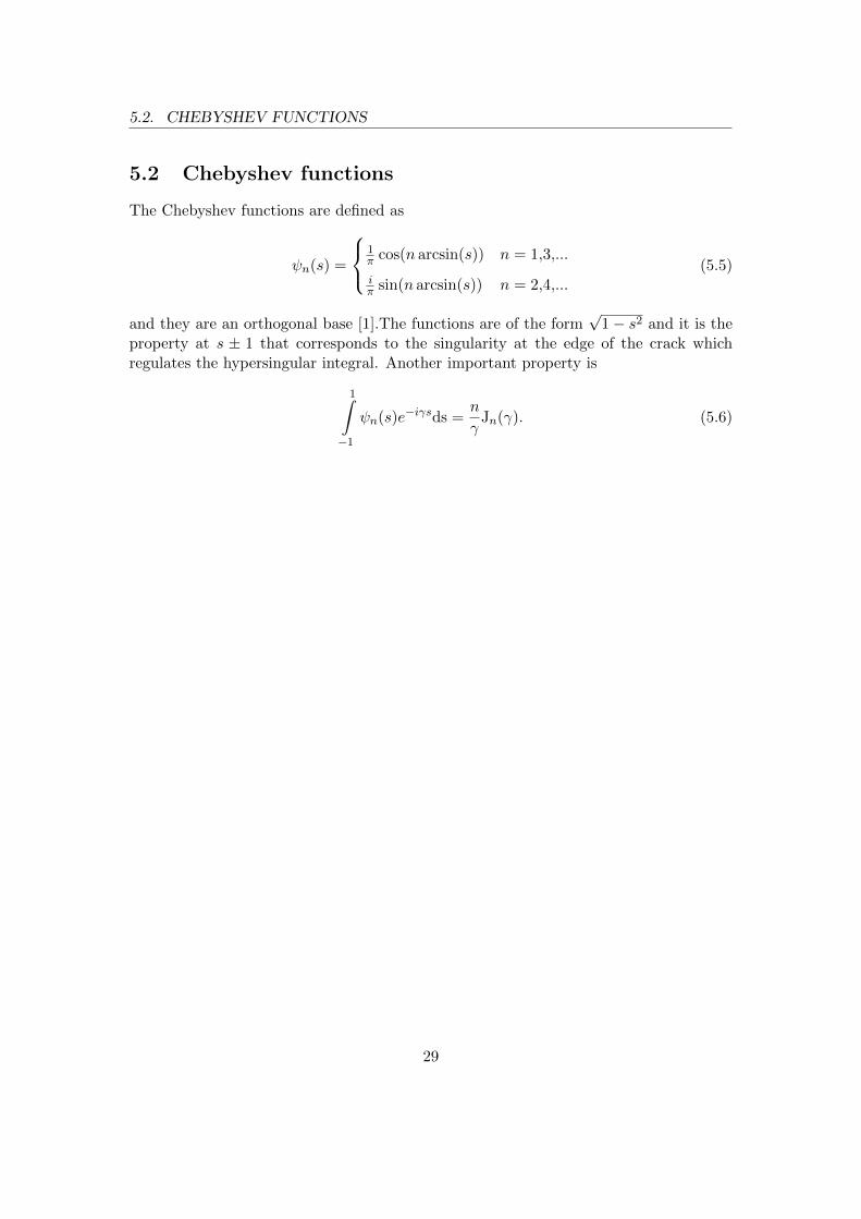
The Chebyshev functions are defined as

ψn(s) =

1π cos(n arcsin(s)) n = 1,3,...

iπ sin(n arcsin(s)) n = 2,4,...

(5.5)

and they are an orthogonal base [1].The functions are of the form√

1− s2 and it is theproperty at s ± 1 that corresponds to the singularity at the edge of the crack whichregulates the hypersingular integral. Another important property is

1∫−1

ψn(s)e−iγsds =n

γJn(γ). (5.6)

29

Bibliography

[1] A. Bostrom, Review of hypersingular integral equation method for crack scattering andapplication to modeling of ultrasonic nondestructive evaluation, Applied MechanicsReviews 56 (4) (2003) 383–405.URL http://link.aip.org/link/?AMR/56/383/1

[2] G. Arfken, Mathematical Methods for Physicists, Academic Press, London, 1970.

[3] P. A. Martin, F. J. Rizzo, Hypersingular integrals: how smooth must the density be?,Int. J. Numer. Methods Eng. 39 (1996) 687–704.URL http://onlinelibrary.wiley.com/doi/10.1002/%28SICI%291097-

0207%2819960229%2939:4%3C687::AID-NME876%3E3.0.CO;2-S/abstract

[4] A. Bostrom, Fundamental Structural Dynamics, 2001.

[5] K. F. Graff, Wave Motion in Elastic Solids, Dover Publications, 1991.

[6] G. B. Folland, Fourier analysis and its applications, The Wadsworth & Brooks/Colemathematics series, Brooks Cole, 1992.

[7] P. M. van den Berg, Transition matrix in acoustic scattering by a strip, Journal ofthe Acoustical Society of America 70 (1981) 615–619.URL http://adsabs.harvard.edu/abs/1981ASAJ...70..615V

[8] A. Bostrom, H. Wirdelius, Ultrasonic probe modeling and nondestructive crack de-tection, Journal of the Acoustical Society of America 97 (5) (1995) 2836–2848.URL http://asadl.org/jasa/resource/1/jasman/v97/i5/p2836_s1

30

http://link.aip.org/link/?AMR/56/383/1

http://onlinelibrary.wiley.com/doi/10.1002/%28SICI%291097-0207%2819960229%2939:4%3C687::AID-NME876%3E3.0.CO;2-S/abstract

http://onlinelibrary.wiley.com/doi/10.1002/%28SICI%291097-0207%2819960229%2939:4%3C687::AID-NME876%3E3.0.CO;2-S/abstract

http://adsabs.harvard.edu/abs/1981ASAJ...70..615V

http://asadl.org/jasa/resource/1/jasman/v97/i5/p2836_s1

Documents

Improving landfill monitoring programs Modeling of ...publications.lib.chalmers.se/records/fulltext/148464.pdf · Improving landfill monitoring programs ... Modeling of ultrasonic