Improving Interpolants for Linear Arithmetic

Ernst Althaus1,2, Bjorn Beber1(B), Joschka Kupilas1,and Christoph Scholl3

1 Max Planck Institute for Informatics, Campus E 14, 66123 Saarbrucken, Germanybbeber@mpi-inf.mpg.de

2 Johannes Gutenberg University, Staudinger Weg 9, 55128 Mainz, Germany3 Albert-Ludwigs-Universitat, Georges Kohler Allee, Gebaude 51,

79110 Freiburg im Breisgau, Germany

Abstract. Craig interpolation for satisfiability modulo theory formulashave come more into focus for applications of formal verification. In thispaper we, introduce a method to reduce the size of linear constraintsused in the description of already computed interpolant in the theory oflinear arithmetic with respect to the number of linear constraints. Wesuccessfully improve interpolants by combining satisfiability modulo the-ory and linear programming in a local search heuristic. Our experimentalresults suggest a lower running time and a larger reduction compared toother methods from the literature.

Keywords: Craig-interpolation · Linear arithmetic · Satisfiabilitymodulo theory · Linear programming

1 Introduction

First efficients methods were introduced for computing such interpolants forBoolean systems out of the resolution proofs from DPLL-based SAT solvers[1,2]. McMillan [2] introduced interpolants to formal verification as over-approximations of state sets.

Due to the fact that such interpolants are in general not unique, manyresearchers try to find good interpolants. The measurement for interpolantsdiffers depending on the context. In Boolean formulas it is often the size ofthe representation of the interpolant, i.e. the size of the And-Inverter-Graphrepresenting the interpolant. In the theory of linear arithmetic with rationalcoefficients LA(Q) the measurement of the number of linear constraints in therepresentation is often used, e.g. in [3] the authors showed that this measure-ment is beneficial for an improved generation of program invariants in softwareverification. This measurement is motivated by the verification of hybrid systemswhere operations are applied on state sets whose complexity strongly dependson the number of linear constraints, e.g. quantifier elimination in the worst-caseleads to a quadratic blow-up of linear constraints after the elimination. Dammet al. showed [4] that such a measurement is the key for avoiding an explosionin the complexity of the state set representation.c© Springer International Publishing Switzerland 2015B. Finkbeiner et al. (Eds.): ATVA 2015, LNCS 9364, pp. 48–63, 2015.DOI: 10.1007/978-3-319-24953-7 5

Improving Interpolants for Linear Arithmetic 49

In this paper we will only consider interpolants for the theory LA(Q). There-fore our measurement for good interpolants is the number of linear constraints.The problem of finding the best interpolant in this sense is NP-hard, which canbe shown by a reduction from k-Polyhedral Separability [5], i.e. given two sets ofpoints P and Q and an integer k, recognize whether there exist k hyperplanesthat separate the sets P and Q through a Boolean formula. Therefore, we willhere present a heuristic approach that simplifies a given interpolant. Addition-ally, there is no known algorithm that can compute reasonable lower bounds forthis problem to measure the quality of an interpolant, so benchmarks exist wherethe initial interpolant is optimal, without a chance of verifying this situation.

Most approaches in this case were done by constructing an interpolant outof the resolution proof and then simplifying the proof by removing or combiningtheory lemmas [4,6], but maintaining the resolution proof correctly. Our app-roach differs in the way that we do not try to maintain the resolution proof. Infact, we only derive the set of linear constraints used in the interpolant by suchproofs and then try to reduce this set in a local search heuristic. The invariantwe preserve is based on an extension of Proposition 3 in [5], i.e. our set of inter-polant constraints L fulfill that for every pair of points a ∈ A and b ∈ B, thereexists a linear constraint l ∈ L such that l separates the points a and b. Theproposition states that then there exists a Boolean formula, i.e. the interpolant,that separates A and B.

The paper is structured as follows: In Sect. 2 we will briefly describe previousmethods to construct interpolants and the data-structure used in our bench-marks. Then we present our approach in Sect. 3, and some optimizations inSect. 4. After that we present the evaluation of our method compared to threedifferent other approaches in Sect. 5.

2 Preliminaries

2.1 Notations

For a point p ∈ Bn × IRm, we denote the first n components, i.e. the Boolean

components, by pB and the last m, i.e. the real components, by pIR. Wedescribe a single linear constraint l by a formula dTx ≤ d0 with rational coef-ficients d0, d1, . . . , dm ∈ Qm+1 over rational variables x1, . . . , xm. For a pointp ∈ B

n × IRm and a linear constraint l, we associate with l(p) the Boolean vari-able that is true, if dT pIR ≤ d0 and false if dT pIR > d0. We write Dx ≤ d0 fora conjunction of u linear constraints over rational variables (x1, . . . , xm)T = xwith D ∈ Qu×m and d0 ∈ Qu.

2.2 Computing Interpolants by Resolution Proofs

A (quantifier-free) formula F in the theory of linear arithmetic with rationalcoefficients (LA(Q)) is a Boolean combination of atoms. Each atom is potentiallya linear constraint with rational coefficients d over a fixed set of rational variables

50 E. Althaus et al.

x1, . . . , xm, denoted by dTx ≤ d0, or a Boolean variable of a fixed set y1, . . . , yn.A literal κ is either an atom or the negation of an atom. A clause is a disjunctionof literals κ1 ∨ · · · ∨ κs. For a set of literals C and a formula F , we denote byC \ F the set containing the literals in C by removing all atoms occurring inF , and by C ↓ F the set of literals created from C by removing all atoms notoccurring in F .

Definition 1 (Craig Interpolant [7]). Let A and B be two formulas, suchthat A ∧ B � ⊥. A Craig interpolant I is a formula such that A � I, I ∧ B � ⊥and the uninterpreted symbols in I occur both in A and B, the free variabels inI can occur freely both in A and B.

Typically an SMT-Solver solves such formulas stepwise, first handling the nonBoolean atoms like Boolean variables and solving this formula with a SATapproach. After finding a satisfiable assignment for the Boolean variables, e.g.κ1 ∧ · · · ∧ κs, the solver starts a decision procedure for the rational variables,i.e. computes if there exists one assignment of x such that all inequalities in theassignment simultaneously imply their given Boolean assignment. If this is notpossible, we call η = {κ1, . . . , κs} a LA(Q)-conflict, the SMT-solver then adds asubset of κ1,∧ · · · ∧ κs described as a clause called LA(Q)-lemma, to its set ofclauses and starts backtracking, this will provide the procedure from selectingthe invalid assignment again. These subsets are often called minimal infeasiblesubsets and are optimized in the way that the number of literals is minimizedbut still maintaining the LA(Q)-unsatisfiability.

Definition 2 (Resolution Proof). Let S = {c1, . . . , ct} be a set of clauses.P = (VP , EP ) is a directed acyclic graph partitioned in inner nodes and leaves.P is a resolution proof of the unsatisfiability of c1 ∧ · · · ∧ ct in LA(Q), if

1. each leaf in P is either a clause in S or a LA(Q)-lemma (corresponding tosome LA(Q)-conflict η);

2. each inner node v in P has exactly two parents vR and vL, such that vR andvL share a common variable p (pivot variable) in the way that p ∈ vL and¬p ∈ vR. We derive v by computing the conjunction of vR ∧ vL;

3. the unique root node r in P is the empty clause.

Let S = {c1, . . . , ct} be a LA(Q)-unsatisfiable set of clauses, (A,B) a disjointpartition of S, and P a proof for the unsatisfiability of S in LA(Q). Then aninterpolant I for (A,B) can be constructed by the following procedure [8]:

Initiate I as a copy of P , we then change the association of the nodesaccordingly.

1. For every leaf vP ∈ P associated with a clause in S,set vI = vP ↓ B, if vP ∈ A, and set vI = �, if vP ∈ B.

2. For every leaf vP ∈ P associated with a LA(Q)-conflict η,set vI = Interpolant(η \ B, η ↓ B).

3. For every inner node vP ∈ P ,set vI = vL

I ∨ vRI if vP /∈ B, and set vI = vL

I ∧ vRI if vP ∈ B.

Improving Interpolants for Linear Arithmetic 51

The unique root node rI then represents the formula of an interpolant of Aand B. Several methods are known to construct LA(Q)-interpolants, e.g. [9],all have in common that they construct a single linear constraint based on theconvex regions given to the function. One basic idea is to use Farkas Lemmato construct a linear constraint separating these convex regions computed bylinear programming. If those calls are handled separately, this will add for eachLA(Q)-conflict in the proof a linear constraint with a fixed normal [6] to theinterpolant, and therefore will lead to a substantial blow up in the complexity. Tofind simpler interpolants the authors in [6] try to combine those calls by enlargingtheir degrees of freedom, i.e. extending the LA(Q)-lemmas and relaxing specificconstraints in the linear program to find shared interpolants for different theorylemmas in one proof.

2.3 Computing Interpolants by DC-Removability Checks

In the description of a formula F we could ask whether it is possible to removeredundant constraints. This is not as straightforward as in the situation of convexpolyhedra. A linear constraint l is redundant for a formula F if there existsa formula G that depends on the same linear constraints except of l and Fand G represents the same predicates. To achieve this we introduce a “don’tcare set” DC for F , which consists of all Boolean configurations which are notLA(Q)-sufficient, and then efficiently construct G, which holds F = G for everyconfiguration not in DC. This method was introduced by [10] and expanded in[11] to compute an interpolant of A and B. Assume we have two disjoint formulasA,B, i.e. A∧B is unsatisfiable. We then set F = A and extend the set DC fromabove by the set ¬A ∧ ¬B. By the usage of the same construction now the newformula G can differ in all regions that are not specified by either A or B. Thisturns the method of redundancy removal in a method of interpolation.

For both the basic approach of constructing an interpolant from a resolutionproof and the reduncancy removal, the fundamental problem is that there is nofreedom in the choice of linear constraints. The approach introduced in [6] ismore flexible, but lacks the fact that it does not notice if a linear constraint isredundant.

2.4 Description of a State Set

A formula A can be interpreted as a specific subset of Bn × IRm, e.g. a represen-tation of a state set. There are several possibilities to describe state sets, e.g. theLinAIG data structure [11] where such formulas are saved as an extension ofa classical And-Inverter-Graph. An And-Inverter-Graphs is a directed, acyclicgraph partitioned in inner nodes and leaves. Each inner node has exactly twopredecessors, representing a logical conjunction. Each leaf represents a Booleanvariable y ∈ B

n or in LinAIGs a lesser-or-equal constraint over the rational vari-ables x ∈ Qm. Additionally, the edges can contain markers indicating a logicalnegation. The formula A is then the association of the unique root.

This representation is also often used as a data structure for resolution proofs.

52 E. Althaus et al.

Our method does not depend on the way the state sets are described, butwe assume that we can negate and intersect state sets and that we can computewhether a state set is non-empty and if so, obtain a point within the state set.All these operations are executable by common SMT solvers. Furthermore, wecan easily create a set of all linear constraints used in the description of thestate set.

Note that the state sets are not in disjunctive normal form, where convexregions would be easily accessible, and a transformation would not be practicabledue to a potentially exponential blow-up in the description.

3 The General Algorithm

The problem we are solving can be briefly described as follows. Let two statesets A,B and an interpolant of these be given. Try to minimize the number oflinear constraints used in the interpolant.

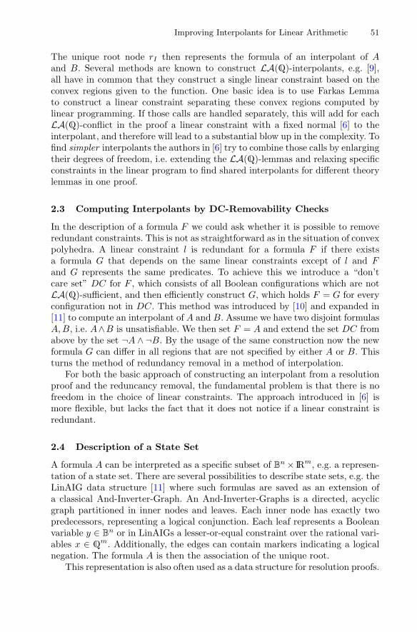
Example 1. Figure 1(a) shows two state sets A,B, with no Boolean complex-ity, i.e. n = 0. One representation of those sets is A = (l1 ∧ l2) ∨ l3 ∨ l4 andB = (l5 ∧ l6) ∨ (l7 ∧ l8). In this case, A itself is an interpolant of A and B.

Our algorithm is based on the following extension of Proposition 3 in [5].

Proposition 1. The set of (linear) constraints L = {L1, . . . , Lh} separates thestate sets A and B through some Boolean formula if and only if for every pairof points p ∈ A and q ∈ B with pB = qB there exists an i (1 ≤ i ≤ h) such thatLi(p) = Li(q).

The proof of the extension is basically the same as the one given in [5] despitetwo differences. Firstly, we have a finite set of (convex) regions instead of points.But since we also used L to construct these regions they behave like points, i.e.the points in such a (convex) region are constant under the associated Booleanvariables. Secondly, in the extension this only holds for pairs of points in the sameBoolean space, since we can distinguish the Boolean spaces by m other Booleanvariables easily in a formula easily. We use this proposition in our algorithm asfollows.

The algorithm iteratively improves the set L by replacing two linear con-straints by one, while preserving the invariant that L satisfy Proposition 1. Thelinear constraints in L are called interpolant constraints. Every new constraintadded to L can be described separately by a linear combination of constraintsin A and B. This lead to the fact that if the initial L only contains constraintsdescribed over local variables of A and B, the output of our algorithm only con-tains such constraints, for details we refer to the linear constraints of the LP(4) and (5) in Sect. 3.4. Hence, our algorithm is a local search heuristic. In thissection, we describe the test whether two linear constraints can be replaced byone and in Sect. 4, we describe some techniques to improve the performance.In particular, we describe our approach to reduce the number of pairs of linearconstraints that are tested. Most approaches are of a heuristic nature.

Improving Interpolants for Linear Arithmetic 53

The interpolant itself is constructed by using the method described inSect. 2.3. We therefore deliver a sufficient set of constraints to construct theinterpolant, so in the constraint minimization the part of finding redundantconstraints can be skipped. This together with the fact that all interpolant con-straints are defined over local variables of A and B lead to the fact that theresulting interpolant is in fact an Craig-Interpolant.

A

B

l3 l2

l1

l4

l5 l7

l6

l8

(a)

a1

b1

l3

l4

l9

(b)

a1

b1

a2b2

l3

l4

l10

(c)

Fig. 1. Running example for our algorithm

3.1 Test Whether One Additional Linear Constraint Is Sufficient

This is the core part of the heuristic, where we determine if we can reduce thesize of the interpolant. It will test if it is possible to substitute two given inter-polant constraints by one new linear constraint l∗. Notice, that when removingtwo interpolant constraints, there will be pairs a ∈ A, b ∈ B of points withaB = bB that can not be distinguished by the remaining interpolant constraintsL, i.e. l(a) = l(b) for all l ∈ L. We will test whether all those pairs of points canbe distinguished by a single new linear constraint.

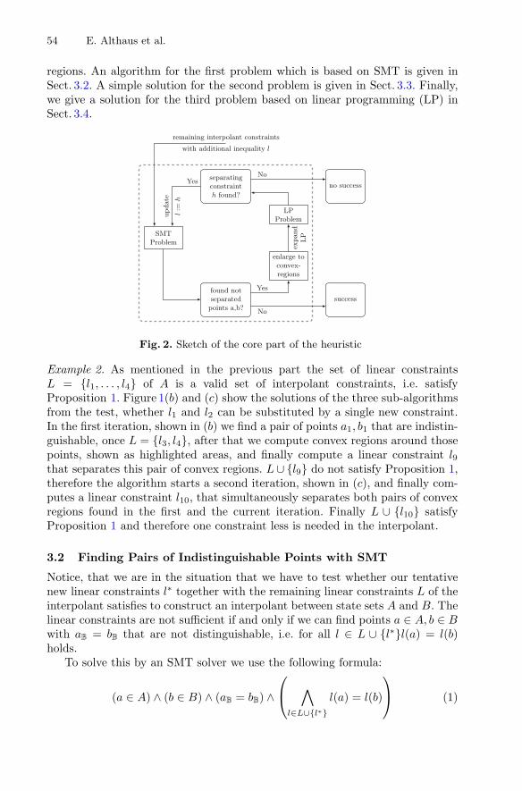
Basically, we iteratively collect such pairs of points and construct a linearconstraint l∗ separating all pairs of points already found, until either all pairsof points can be distinguished with the additional help of l∗ or no such linearconstraint can be found. Figure 2 gives a sketch of the algorithm.

In order to guarantee termination, it does not satisfy to collect pairs of points,as there can be an infinite number. Therefore, we construct convex regions Ca

and Cb around the points a and b described only by constraints known to thesystem, i.e. for Ca we only use linear constraints used in the description of A andadditionally all remaining interpolant constraints. The convex sets are containedin the respective sets, i.e. Ca ⊆ A and Cb ⊆ B. Since there are only a finitenumber of linear constraints in the description of the state sets and interpolantconstraints, there are only a finite number of possible convex sets describable bythese constraints. This lead to a termination of this part of the algorithm in afinite number of steps.

Hence, we need three sub-algorithms. One for finding pairs of points that cannot be distinguished, one for constructing the convex regions around them, andone for constructing a linear constraint separating a given set of pairs of convex

54 E. Althaus et al.

regions. An algorithm for the first problem which is based on SMT is given inSect. 3.2. A simple solution for the second problem is given in Sect. 3.3. Finally,we give a solution for the third problem based on linear programming (LP) inSect. 3.4.

separatingconstrainth found?

no success

LPProblem

SMTProblem

enlarge toconvex-regions

found notseparatedpoints a,b?

success

No

Yesex

pand

LP

Yes

update

l:=

hNo

remaining interpolant constraints

with additional inequality l

Fig. 2. Sketch of the core part of the heuristic

Example 2. As mentioned in the previous part the set of linear constraintsL = {l1, . . . , l4} of A is a valid set of interpolant constraints, i.e. satisfyProposition 1. Figure 1(b) and (c) show the solutions of the three sub-algorithmsfrom the test, whether l1 and l2 can be substituted by a single new constraint.In the first iteration, shown in (b) we find a pair of points a1, b1 that are indistin-guishable, once L = {l3, l4}, after that we compute convex regions around thosepoints, shown as highlighted areas, and finally compute a linear constraint l9that separates this pair of convex regions. L ∪ {l9} do not satisfy Proposition 1,therefore the algorithm starts a second iteration, shown in (c), and finally com-putes a linear constraint l10, that simultaneously separates both pairs of convexregions found in the first and the current iteration. Finally L ∪ {l10} satisfyProposition 1 and therefore one constraint less is needed in the interpolant.

3.2 Finding Pairs of Indistinguishable Points with SMT

Notice, that we are in the situation that we have to test whether our tentativenew linear constraints l∗ together with the remaining linear constraints L of theinterpolant satisfies to construct an interpolant between state sets A and B. Thelinear constraints are not sufficient if and only if we can find points a ∈ A, b ∈ Bwith aB = bB that are not distinguishable, i.e. for all l ∈ L ∪ {l∗}l(a) = l(b)holds.

To solve this by an SMT solver we use the following formula:

(a ∈ A) ∧ (b ∈ B) ∧ (aB = bB) ∧⎛⎝ ∧

l∈L∪{l∗}l(a) = l(b)

⎞⎠ (1)

Improving Interpolants for Linear Arithmetic 55

Either we found a valid solution and therefore two points a, b that are not sepa-rable by any linear constraint in L∪{l∗} or we found that L∪{l∗} is a valid set ofinterpolant constraints. The problem has only minor changes in every iteration,because we only substitute the old condition l∗(p) = l∗(q) with an updated linearconstraint l∗. This gives us the opportunity to use the advantage of incrementalSMT.

3.3 Enlarge Pairs of Indistinguishable Points to Convex Regions

If we have found a pair of points a, b as described in the previous section, wewant to find a set of points Ca ⊆ A around a that is preferably large, such thatno point in Ca can be distinguished from b and vice versa.

We achieve this by computing convex regions around a, such that all pointswithin Ca are equal with respect to all linear constraints in L\{l∗} and all linearconstraints used in the description of A.

For computing Ca test for every linear constraint l that is used in the descrip-tion of A, if a satisfies this linear constraint, i.e. we compute l(a). We thereforecollect linear constraints in a set C. We add l to C when l(a) is true, or ¬ l ifl(a) is false. After evaluating that for every linear constraint in A, we computethe same for every interpolant constraint. We do not use the current l∗ in thedescription of the convex region, since we change this constraint in the next step,where we search for a new candidate. Ca is then computed as a conjunction ofall constraints in C.

3.4 Finding a Linear Constraint Separating Pairs of ConvexRegions with LP

We try to find a solution to this problem by constructing a linear program whosesolution represents a separating linear constraint. The LP does not solve theproblem in general, as it will fix all convex regions of A on one side and the convexregions of B on the other side, which is not necessarily required. Furthermore,it assumes that all inequalities in A and B are non-strict, i.e. convex regions areenlarged by their boundary. Both deficiencies are handled heuristically later. Weuse an LP-solver that handles rational arithmetic as errors in the coefficientsprevent the algorithm from termination since we could be forced to separate thesame pair of convex region multiple times.

The construction of the LP is similar to the one that computes the linearconstraints in resolution proofs, hence based on Farkas’ Lemma. We expandedthe approach to separate multiple pairs of convex regions.

Therefore, we define the variables d ∈ Qm and d0 ∈ Q that describe thenew linear constraint l∗ in the form dTx ≤ d0. Pairs of convex sets (Ai, Bi)for i ∈ {1, . . . , k}, which are present in the k-th iteration of the LP-problem forfinding a new constraint for one test described in Sect. 3.1, all constructed bythe enlargement of points to convex regions described in Sect. 3.3. The constraintdTx ≤ d0 is implied by Ai, if there is a non-negative linear combination of theinequalities of Ai leading to dTx ≤ d0. Similarly, the constraint aTx > b is

56 E. Althaus et al.

implied by Bi, if there is a positive ε such that there is a non-positive linearcombination of the inequalities of Bi leading to dTx ≥ d0 + ε. All constraintscan easily be formulated as linear constraints.

A detailed description of the LP is given in the appendix. If the LP is solvableand ε > 0 the computed linear constraint l∗ separates each pair of convex regions.

Extension to Non-Closed Polyhedra. Obviously, the former statement isalso true in the case that some of the inequalities are strict. When the LP issolvable but ε = 0, at least one of the convex regions of each set touches theinequality if all inequalities are non-strict. Hence, the LP solution does not givea linear constraint in this case, as the negation of the non-strict inequality isnot implied by one convex set of B and its strict version is not implied by oneconvex set of A. If there are strict inequalities in the description of the convexregions, we test whether the computed linear constraint still separates the convexregions either in the non-strict or in the strict version. This is done by computingif the non-strict or the strict version is a valid choice for each pair. Only if asolution is valid for every pair it is a solution for the problem. Details are givenin Section B in the appendix. Alternatively, a linear program that is forced touse a strict inequality of the right-hand side of the linear combination evaluatesif d0 can be used.

Greedy Approach. The LP is trying to separate all regions by always forcingAi on one side of l∗ and all Bi on the other side of l∗. This is more than weactually need in order to satisfy Proposition 1. So we expand our LP problemby a greedy approach as follows. Assume we find a linear constraint separatingthe pairs

(Ai, Bi

)for the first k − 1 convex pairs, but the LP does not find a

solution when trying to set Ak on the one side and Bk on the other. Then wetry to switch the sides of Ak and Bk, i.e. we modify the variable bounds andthe constraints concerning the last added pair of regions, such that the convexregions will change the sides on l∗.

This is a greedy approach, as we only change the positions of the convexregions of the last iteration.

The LP and Proposition 2 given in Section B in the appendix can be adoptedeasily for this greedy approach.

4 Optimizations

Our main goal with the optimizations is to reduce the number of tested pairsof linear constraints to a reasonable amount. For this goal, we first introducethe concept of Non-Redundancy-Certificate-points (NRC-points) for interpolantconstraints, which are then used to choose interesting candidates of pairs of lin-ear constraints. The idea behind this heuristic is, that it is more likely to combineconstraints when they are needed to separate the same regions. There will besituations where we will not choose the correct pair. To check the potency of the

Improving Interpolants for Linear Arithmetic 57

heuristic choice of specific pairs and the overall heuristical algorithm we com-puted all benchmarks in Sect. 5 with the heuristical choice and by testing everypair of interpolant constraints. Furthermore, we give some other optimizationsto the general approach.

NRC-Points. An NRC-Point (a, b) is a pair of points, where a ∈ A and b ∈ Bare only distinguishable by one interpolant constraint h and are indistinguishablefor every other interpolant constraint, we call (a, b) a NRC-point of h. Formally,an NRC-point (a, b) of h is a solution of the formula

(a ∈ A) ∧ (b ∈ B) ∧ (aB = bB) ∧⎛⎝ ∧

l∈L\hl(a) = l(b)

⎞⎠ . (2)

Since there can be more than one NRC-point of h, we first solve (2), then wecompute convex regions Ca, Cb around a and b, with the method described inSect. 3.3. After this, we solve (2) with the additional conjunction, that (a /∈Ca) ∧ (b /∈ Cb). This can be done multiple times, and with the advantage of anincremental SMT since we only add clauses to the formula.

It is worth mentioning that the search for the NRC-points detects if aninterpolant constraint is redundant, i.e. it is not needed to fulfill Proposition 1.This is the case, when (2) is not satisfiable in the first iteration. When thisoccurs, we delete the inequality from the interpolant constraints. To keep thecomputational effort low, we only compute a maximum of three NRC-points foreach interpolant constraint, this is motivated by experimental results.

Example 3. Consider Example 2, we want to compute all NRC-points for l3.Therefore we search for points (a3, b3), that are a solution to the problem(a3 ∈ A) ∧ (b3 ∈ B) ∧ (

∧i∈{1,2,4} li(a3) = li(b3)). The pair (a3, b3) is shown in

Fig. 3(a). The highlighted areas are again the convex regions built around thepoints a3, b3. There is no other solution that is not in the convex regions, there-fore (a3, b3) is the only NRC-point for l3. Additionally it is easy to see in Fig. 1,that the pair (a1, b1) is an NRC-point of l1, and (a2, b2) an NRC-point of l2.

The Choice of Interesting Pairs of Inequalities. After we calculated theNRC-points for every interpolant constraint, we compare the constructed convexregions around these points. A pair of inequalities (s, t) is chosen by our heuristic,if there exist two NRC-points (as, bs) and (at, bt) for interpolant constraints s andt, such that either as and at or bs and bt are equal in respect to all l ∈ L \ {s, t}.

In this case, our heuristic chooses the pair (s, t) as a pair that is promising,and therefore will be tested by the method described in Sect. 3.1.

If it was possible to improve the interpolant by testing the pair (s, t), all otherconstraints that where chosen to be tested with either s or t are then tested withthe newly found interpolant constraint.

Example 4. Consider Example 3, we already computed NRC-points for l1, l2and l3. The heuristic for interesting pairs now compares these points, i.e. the

58 E. Althaus et al.

a3

b3

l3 l2

l1

l4

(a)

a1

b1

a2 b2

l3

l4

(b)

a1

b1

l3

l4

a3

b3

(c)

Fig. 3. Example of NRC-points and the heuristic choice of pairs.

convex regions around these points only build by interpolant constraints. InFig. 3(b), we see that the convex regions around a1 and a2 are the same, theheuristic therefore chooses the pair l1, l2 as a promising candidate. The heuristicdoes not choose the pair l1, l3 since none of the convex regions are equal as wecan see in Fig. 3(c).

Using NRC-Points to Save SMT-Calls. Assume we want to replace theinterpolant constraints l1 and l2 by a new linear constraint l∗. The algorithm inSect. 3.1 would first compute a pair of points, that is now not separable. Withthe precomputation of NRC-points, we can skip this since we already have atleast two pairs of convex regions at hand that need to be distinguished by l∗.

5 Experimental Results

We implemented our algorithm in the C++ language, using Yices [12] to solvethe SMT problems and QSopt-Exact [13] to solve the rational LP problems. Allcomputations were done on a single core of an Intel I7 with 3.20 GHz, and amemory limit of 2 GB. The maximal time used for a computation of a singleinterpolant for a method was 15minutes, the average overall was around 2 s.The benchmarks are intermediate state sets of over 150 different model checkerruns, mainly two different categories of models. We tested 62 models of thecategory Flap/Slat System (FS), during take-off (and landing) flaps and slatsof the aircraft are extended to generate more lift at low velocity and have tobe retracted in time as they are not robust enough for high velocities. Themodels have different numbers of flaps/slats, explained in more detail in [15].Another 90 models of the category of ACC, where a controllers objective is toset the acceleration of the controlled car to make it reach the goal velocity in adistance equal to or greater than the goal distance. Additionally, we tested 15other models of other categories. Damm et al. [4] provided the model checkerand models, which created the intermediate state sets. Independent of the modelwhich is tested the intermediate state sets are divided in two different classes.In the first class, formula A describes a state set and formula B describes the

Improving Interpolants for Linear Arithmetic 59

negation of a bloated version of A. This is used in the model checker, if thedescriptions of the state sets become too difficult. Hence, we look for a state setwith a simpler description that is slightly larger than the given state set. Dueto the bloating factor this will lead to different degrees of freedom. In all ourbenchmarks the bloating factor for each linear constraint was set to 10%, soevery linear constraint of the bloated state set is pushed by 10% of the totalvariable range of all variables used in the constraint, which is applicable, sinceall benchmarks are bounded in every variable. The second class comes from theso-called abstraction refinement, where specific points are excluded in a previouscomputed interpolant computation. In this set of benchmarks the two state setsA and B “touch” each other, i.e. they use the same linear constraint in differentorientations.

All benchmarks are compared with Constraint Minimization [4], which basi-cally removes redundant constraints out of the description, a version of SimpleInterpolants [6], which creates shared constraints in the proof, and the standardinterpolation method of MathSat [14]. To compare the quality of the solutionsof Simple interpolants and MathSat we additionally executed a Constraint Min-imization at the end of their computation. We were not able to compare ourapproach with the method described in [3], as their description of the state setsdiffers from ours.

We implemented four types of our approach. Approaches g all and n all testall pairs of linear constraints, while g h and n h only test pairs of interpolantconstraints selected by our heuristic described in Sect. 3.4. Further g all and g huse the greedy approach described in Sect. 3.4, while n all and n h do not useit. A computed interpolant obtained by Constraint Minimization was used tocompute the initial set of interpolant constraints L.

Table 1 shows a comparison of gall, nall, gh, nhs, Simple Interpolants (SI),MathSat (MS), and Constraint Minimization (CM).

The benchmarks are all sorted by categories (FS, ACC, other models) andclasses (bloated, refinement). The key specifics of each benchmarks are givenwith the number instances, the number of Boolean variables n, and the num-ber of real variables m in the table. To compare the approaches, we state theaverage number of linear constraints (# LC) and its variance (var. # LC). Thenthe relative size of the interpolant (rel. # LC) is compared to the approach ofConstraint Minimization, since this method only removes redundant constraints.Additionally, we state the number of instances where the method improved theinterpolant (# better), again compared to the Constraint Minimization. In thecell of the Constraint Minimization “# better” states the number of instanceswhere no method constructed an interpolant better than the one computed bythe Constraint Minimization. At last, the average runtime (time) of each methodis stated.

From the table we can see that most of the benchmarks in the refinementcontext independent of the model could usually not be improved by any method.The distinct test where this can be seen is ACC - refinement. In this set of bench-marks for every of the 180 instances all methods computed an equal interpolant.We assume that this is the result of the fact that the state sets “touch” each

60 E. Althaus et al.

Table 1. Experimental results

gall nall gh nh SI MS CM

FS - bloated (2255 instances, n ∈ {0, . . . , 34}, m ∈ {1, . . . , 3})#LC 6.18 6.30 6.76 6.79 7.33 7.39 7.43

var. #LC 7.72 8.51 10.434 10.66 9.78 9.70 9.97

rel. #LC 0.83 0.85 0.90 0.90 0.99 1.00 1

#better 1533 1453 969 938 336 196 717

time 3.14 s 2.35 s 0.92 s 0.82 s 1.78 s 0.83 s 0.37 s

FS - refinement (915 instances, n ∈ {0, . . . , 36}, m ∈ {2, . . . , 3})#LC 8.00 8.01 8.12 8.12 8.22 8.23 8.22

var. #LC 11.28 11.32 11.19 11.21 11.22 11.23 11.13

rel. #LC 0.97 0.97 0.98 0.99 1.00 1.00 1

#better 138 134 81 79 15 10 776

time 2.59 s 2.10 s 0.69 s 0.64 s 0.95 s 0.62 s 0.30 s

ACC - bloated (1575 instances, n ∈ {0, . . . , 7}, m ∈ {3, . . . , 5})#LC 2.28 2.28 2.51 2.51 4.41 5.71 5.54

var. #LC 0.38 0.38 0.25 0.25 2.19 11.84 6.06

rel. #LC 0.51 0.51 0.55 0.55 0.87 1.01 1

#better 1305 1305 1305 1305 724 258 270

time 2.60 s 2.09 s 1.33 s 1.12 s 0.35 s 0.24 s 0.24 s

ACC - refinement (180 instances, n ∈ {4, . . . , 7}, m ∈ {7})#LC 3 3 3 3 3 3 3

var. #LC 0 0 0 0 0 0 0

rel. #LC 1 1 1 1 1 1 1

#better 0 0 0 0 0 0 180

time 0.36 s 0.29 s 0.34 s 0.26 s 0.06 s 0.04 s 0.06 s

other models - bloated (740 instances, n ∈ {0, . . . , 31}, m ∈ {1, . . . , 5})#LC 7.32 7.43 8.13 8.16 8.28 8.47 8.50

var. #LC 13.84 14.83 18.32 18.72 19.78 20.54 20.16

rel. #LC 0.87 0.88 0.95 0.95 1.00 1.00 1

#better 464 435 209 196 64 64 276

time 7.77 s 6.30 s 3.48 s 3.40 s 11.33 s 8.36 s 1.83 s

other models - refinement (96 instances, n ∈ {4, . . . , 24}, m ∈ {2, . . . , 3})#LC 12.09 12.11 12.11 12.13 12.31 12.34 12.19

var. #LC 21.62 21.79 21.87 21.84 22.32 22.61 21.73

rel. #LC 0.99 0.99 0.99 0.99 1.01 1.01 1

#better 9 7 7 6 2 2 86

time 8.30 s 6.65 s 2.37 s 2.30 s 11.78 s 8.73 s 1.23 s

Improving Interpolants for Linear Arithmetic 61

other and therefore reduce the degree of freedom. On the other hand, all of ouralgorithms were able to improve most of the bloated benchmarks. Again theobvious test where this can be seen is in the ACC models. There, all of ourmethods could improve 1305 of 1575 instances, with an overall relative improve-ment of 49% for the algorithms that tested every pair of interpolant constraints,and 45% for the two algorithms that tested only interesting pairs computed byour heuristic.

The experiments also indicate that our greedy approach for the LP problemis not often helpful in improving interpolants, i.e. there were only 162 of total5761 instances where the greedy algorithm (gall, gtps) was better than the appro-priate normal algorithm (nall, ntps). Overall, our algorithm ntps achieves the bestratio in improving interpolants compared to the time effort, with a overall factorof ∼4.71 in exceeded running time and an improvement of around 20%.

6 Conclusion and Further Research

In this paper, we showed how the number of linear constraints in interpolants forlinear arithmetic can be reduced by a fair amount. The experiments showed thatin the context of intermediate state sets in hybrid model checking the success ofour algorithm closely related to the model in which this problem occurs. Further,we plan to improve our running times by replacing the rational LP solver by astate of the art LP solver and use rational arithmetic only to verify the feasibilityof the solutions. Additionally, we want to improve our heuristic for the choiceof “interesting” pairs of interpolant constraints. Furthermore, we will try tocompute lower bounds for the amount of interpolant constraints needed in thiscontext.

Acknowledgment. The results presented in this paper were developed in the contextof the Transregional Collaborative Research Center ‘Automatic Verification and Analy-sis of Complex Systems’ (SFB/TR 14 AVACS) supported by the German ResearchCouncil (DFG). We worked in close coorperation with our colleagues from the ’FirstOrder Model Checking Team’ within the subproject H3 and we would like to thank W.Damm, B. Wirtz, W. Hagemann, and A. Rakow from the University of Oldenburg, U.Waldmann from the Max Planck Institute for Informatics at Saarbrucken and S. Dischfrom the University of Freiburg for numerous ideas and discussions

A Detailed Description of the Linear Program

Recall the variables given in Sect. 3.4. Let Ai, Bi be the convex sets of the i-thiteration, constructed by sAi , respectively sBi , conjunctions of linear constraints.Then Ai is formally defined by Ai =

{x ∈ R

m| Aix ≤ αi}, with Ai ∈ Qm×sAi

and Bi ={x ∈ R

m| Bix ≤ βi}, with Bi ∈ Qm×sBi . We additionally introduce

sAi variables λi and sBi variables μi for every iteration i ∈ {1, . . . , k}.We look for an inequality that maximizes a simple measure of the distance

of the constructed inequality to the convex regions. We do this by subtracting

62 E. Althaus et al.

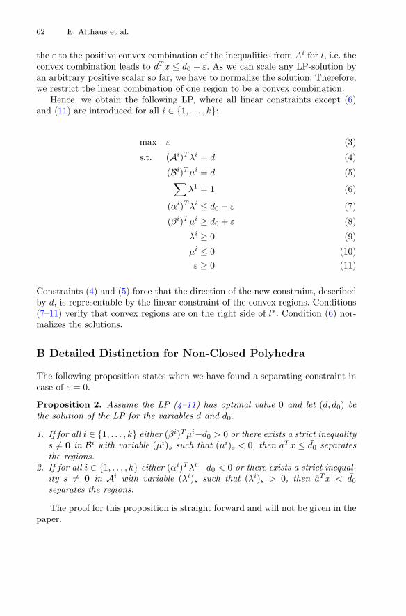
the ε to the positive convex combination of the inequalities from Ai for l, i.e. theconvex combination leads to dTx ≤ d0 − ε. As we can scale any LP-solution byan arbitrary positive scalar so far, we have to normalize the solution. Therefore,we restrict the linear combination of one region to be a convex combination.

Hence, we obtain the following LP, where all linear constraints except (6)and (11) are introduced for all i ∈ {1, . . . , k}:

max ε (3)

s.t. (Ai)Tλi = d (4)

(Bi)Tμi = d (5)∑λ1 = 1 (6)

(αi)Tλi ≤ d0 − ε (7)

(βi)Tμi ≥ d0 + ε (8)

λi ≥ 0 (9)

μi ≤ 0 (10)ε ≥ 0 (11)

Constraints (4) and (5) force that the direction of the new constraint, describedby d, is representable by the linear constraint of the convex regions. Conditions(7–11) verify that convex regions are on the right side of l∗. Condition (6) nor-malizes the solutions.

B Detailed Distinction for Non-Closed Polyhedra

The following proposition states when we have found a separating constraint incase of ε = 0.

Proposition 2. Assume the LP (4–11) has optimal value 0 and let (d, d0) bethe solution of the LP for the variables d and d0.

1. If for all i ∈ {1, . . . , k} either (βi)Tμi−d0 > 0 or there exists a strict inequalitys = 0 in Bi with variable (μi)s such that (μi)s < 0, then aTx ≤ d0 separatesthe regions.

2. If for all i ∈ {1, . . . , k} either (αi)Tλi−d0 < 0 or there exists a strict inequal-ity s = 0 in Ai with variable (λi)s such that (λi)s > 0, then aTx < d0separates the regions.

The proof for this proposition is straight forward and will not be given in thepaper.

Improving Interpolants for Linear Arithmetic 63

References

1. Pudlak, P.: Lower bounds for resolution and cutting plane proofs and monotonecomputations. J. Symbolic Logic 62(3), 981–998 (1997)

2. McMillan, K.L.: Interpolation and sat-based model checking. In: Hunt Jr., W.A.,Somenzi, F. (eds.) CAV 2003. LNCS, vol. 2725, pp. 1–13. Springer, Heidelberg(2003)

3. Albarghouthi, A., McMillan, K.L.: Beautiful interpolants. In: Sharygina, N., Veith,H. (eds.) CAV 2013. LNCS, vol. 8044, pp. 313–329. Springer, Heidelberg (2013)

4. Damm, W., Dierks, H., Disch, S., Hagemann, W., Pigorsch, F., Scholl, C.,Waldmann, U., Wirtz, B.: Exact and fully symbolic verification of linear hybridautomata with large discrete state spaces. Sci. Comput. Program. 77(10–11), 1122–1150 (2012)

5. Megiddo, N.: On the complexity of polyhedral separability. Discrete Comput.Geom. 3(1), 325–337 (1988)

6. Scholl, C., Pigorsch, F., Disch, S., Althaus, E.: Simple interpolants for linear arith-metic. In: Design, Automation and Test in Europe Conference and Exhibition(DATE), 2014, pp. 1–6. IEEE (2014)

7. William, C.: Three uses of the Herbrand-Gentzen theorem in relating model theoryand proof theory. J. Symbolic Logic 22(03), 269–285 (1957)

8. McMillan, K.L.: An interpolating theorem prover. Theoret. Comput. Sci. 345(1),101–121 (2005)

9. Rybalchenko, A., Sofronie-Stokkermans, V.: Constraint solving for interpolation.In: Cook, B., Podelski, A. (eds.) VMCAI 2007. LNCS, vol. 4349, pp. 346–362.Springer, Heidelberg (2007)

10. Scholl, C., Disch, S., Pigorsch, F., Kupferschmid, S.: Using an SMT solver andcraig interpolation to detect and remove redundant linear constraints in repre-sentations of non-convex polyhedra. In: Proceedings of the Joint Workshops of the6th International Workshop on Satisfiability Modulo Theories and 1st InternationalWorkshop on Bit-Precise Reasoning, pp. 18–26. ACM (2008)

11. Damm, W., Disch, S., Hungar, H., Jacobs, S., Pang, J., Pigorsch, F., Scholl, C.,Waldmann, U., Wirtz, B.: Exact state set representations in the verification oflinear hybrid systems with large discrete state space. In: Namjoshi, K.S., Yoneda,T., Higashino, T., Okamura, Y. (eds.) ATVA 2007. LNCS, vol. 4762, pp. 425–440.Springer, Heidelberg (2007)

12. Dutertre, B., De Moura, L.: The yices SMT solver (2006). http://yices.csl.sri.com/tool-paper.pdf

13. Applegate, D.L., Cook, W., Dash, S., Espinoza, D.G.: Exact solutions to linearprogramming problems. Oper. Res. Lett. 35(6), 693–699 (2007)

14. Griggio, A.: A practical approach to satisfiability modulo linear integer arithmetic.JSAT 8, 1–27 (2012)

15. Rakow, A.: Flap/Slat System. http://www.avacs.org/fileadmin/Benchmarks/Open/FlapSlatSystem.pdf