Feature Report

Improvements to the performance of basic, regulatory control systems have a great return on investment and are some of the least expensive control im-

provements to make [1]. Control valves have a major impact on control loop per-formance and, therefore, improvements in valve performance can have significant economic benefits. This article shows how poor control-valve performance can be identified and corrected to achieve these benefits. A plant example is used to dem-onstrate these methods.

In addition to corrective actions, com-prehensive control-valve specifications,

based on process requirements for new applications, can provide quicker plant startups and immediate economic sav-ings.

The control valve systemIn this article, the control valve is con-sidered to be a dynamic system, from the input signal through to the flow coeffi-cient that determines the fluid flowrate through the pipe. The control valve sys-tem includes the valve, actuator, motion conversion mechanism, stem or shaft, closure member (such as plug, ball or disc) and other valve accessories. Exam-

ples of valve accessories include current to pressure transducer (I/P), positioner, air booster relay, dampener and air set. So, when a change of the input signal to the control valve occurs, the I/P and posi-tioner must respond to move the actuator, which must move the motion conversion mechanism, which must move the stem or shaft, which must move the closure member, which must change the flow co-efficient. As you can see, there is a lot of opportunity for problems.

The key to control valve performance is creating a measurable change in flow through the valve in response to small,

Feature Report

James BeallEmerson Process Management

The control valve is a focal point for

improvements to both process performance

and economics

Improving Control Valve Performance

Input

a < resolution ≤ b

c ≤ dead band < d

c d

TimeDynamics are not shown

Am

plit

ud

e

ab

Output

FIGURE 1. Dead band and resolution, il-lustrated here, are key static-response param-eters for control valves

www.che.com

October 2010

Feature Report

42 CHEMICAL ENGINEERING WWW.CHE.COM OCTOBER 2010

input step changes (1% and less). A change in flow indicates that the valve’s flow coef-ficient has actually changed in response to a change in the input signal. If the actual flow through the control valve is not avail-able or is not measured, then the valve stem, shaft or actuator movement may be used to estimate the response of the valve. However, the movement of the valve stem, shaft or actuator may not be an accurate representation of the actual change in the valve flow coefficient for all changes of the input signal to the valve. For example, the inboard end of the shaft of a rotary valve might move in response to a change in the input to the control valve but the actual flow coefficient might not change because shaft windup occurs and the valve closure member does not move. In some cases the actuator position may be used to measure the control valve response and this adds yet another potential discrepancy between the input to the control valve and the ac-tual change in the valve flow coefficient. However, it is important to note that the response of the valve flow coefficient can be no better than that of the stem, shaft or actuator position.

Control valve performanceThe performance of a control loop will be limited by the poorest performing compo-nent in the loop, such as the transmitter, the controller tuning or the final control element. Note that for most control loops, the final control element is a control valve. One study of over 5,000 control loops re-vealed that poor control-valve perfor-mance negatively impacted control loop performance on 30% of these loops [2].

Important aspects of control valve per-

formance include the static response, the dynamic response and the valve trim size and flow characteristics. The Interna-tional Society of Automation’s (ISA) tech-nical reference, ANSI-ISA-TR75-25-02, explains the concepts of control-valve static- and dynamic-response metrics [3]. ISA standard ANSI-ISA-75-25-01 is a test procedure to measure the static and dy-namic response of a control valve system [4]. However, this standard does not pre-scribe what response requirements should be specified in order to achieve the desired control-valve performance for a particular application. The EnTech Control Valve Dynamic Specification V3.0 provides guidance on specifying the static- and dynamic-response parameters and the valve trim size and flow characteristics to achieve the desired process control perfor-mance [5].Static response. So, what are these con-trol-valve response parameters and what do they mean to process control perfor-

mance? Static response refers to measure-ments that are made with data points that are recorded after the device has come to a rest. Key static-response parameters for control valves include travel gain, dead band and resolution [3]. Travel gain, Gx, is the change in closure member position divided by the change in input signal, both expressed in percentage of full span. The closure member is the portion of the valve trim that moves to change the flow through the valve. If there is no signal characterization inside the valve system, the travel gain should be 1.0. In other words, travel gain is a measure of how well the valve system positions its closure member compared to the input signal.

Dead band is defined as “the range through which an input signal may be varied, with reversal of direction, with-out initiating an observable change in output signal” [6]. With respect to control valve performance, if the process control-ler attempts to reverse the position of the control valve, the valve will not begin to move until after the controller output has reversed an amount greater than the dead band. A large dead band will negatively impact control performance.

Another key static-response parameter is resolution. Resolution is defined as “the smallest step increment of input signal in one direction for which movement of the output is observed” [3]. Resolution will cause the control valve to move in discrete steps in response to small, step input changes in the same direction. This occurs as the valve travel sticks for the amount of resolution after completing the previous step in the same direction. Similar to dead band, a larger resolution will negatively

Inp

ut,

stem

%

350 10

Travel gain = 0.91 Time to steady state, Tss = 18.3 s

Time, s

Final steady stateaverage values

input = 37.84, stem = 37.65

Initial overshoot to 38.11 = 23%

Stem

Input

86.5% of response, T86 = 2.06 s

Dead time Td =1.6 s

Initial steady state average values, input and stem = 35.67

20 30

36

37

38

39

LV-2

R-1 LC-1

LC-2

LV-1

R-2

Variation of valve positionrepresents variation in flow to downstream reactor

Level variation ~ 20%

~ 120 days

FIGURE 2. This graphs shows the response of a control valve to a step input (reprinted with permission from EnTech Control Valve Dynamic Specification V3.0)

FIGURE 3. In this plant example, the level controller output went directly to the control valve positioner

FIGURE 4. In the plant example, the reactor level was not well-controlled

impact control performance. Figure 1 il-lustrates dead band and resolution.Dynamic response. The second aspect of control valve performance is the dy-namic response. Dynamic response is the time-dependant response resulting from a time-varying input signal [4], and in-cludes dead time, step response time and overshoot. The ISA technical reference ANSI-ISA-TR75-25-02 [3] provides the following definitions for these dynamic response parameters:• Dead time — The time after the initia-

tion of an input change and before the start of the resulting observable re-sponse

• Step response time — The interval of time between initiation of an input-sig-nal step change and the moment that the dynamic response reaches 86.5% of its full, steady state value. The step response time includes the dead time before the dynamic response

• Overshoot — The amount by which a step response exceeds its final, steady state value (refer to Figure 24 of ANSI/ISA-51.1-1979 (R1993)). Usually expressed as a percentage of the full change in steady state value

Figure 2 shows the dead time, step re-sponse time and overshoot for a control valve response to a step input change. In this case, stem position in percent of travel is used as the control valve “output”.

It is important to note that the dynamic response of a control valve varies depend-ing upon the size of the input step change. Four “ranges” of step sizes to help under-stand the static- and dynamic-response metrics are defined in the technical refer-ence [3]: • Region 1 is defined as small input steps

that result in no measurable movement of the closure member within the speci-fied wait time

• Region 2 is defined as the input step changes that are large enough to re-sult in some control-valve response with each input signal change, but the response does not satisfy the require-ments of the specified time and linear-ity

• Region 3 is defined as step changes that are large enough to result in flow coef-ficient changes, which satisfy both the specified maximum response time and the specified maximum linearity

• Region 4 is defined as input steps larger than in Region 3 where the specified magnitude-response linearity is satis-fied but the specified response time is exceeded

Region 1 is directly related to dead band and resolution. Region 2 is a highly non-linear region that causes performance problems and should be minimized. Region 3 is the range of input movements that are important to control performance. The dy-namic response parameters, dead time and response time, are applicable in this region. Regions 1, 2, 3 and 4 correspond to regions A, B, C and D as defined in Ref. 5.

Process control issuesA very important aspect of process con-trol is the process gain, which is defined as the ratio of the change in process vari-able to the change in controller output that caused the change. For good process

control, it is desirable for the process gain to be within a certain range and to be con-sistent throughout the operating range of the valve. If the process gain is too high, valve non-linearities are amplified by the process gain and process control performance deteriorates. If the process gain is too low, the range of control is re-duced. Changes in the process gain over the range of operation result in poorly performing regions in the closed-loop con-troller response. Two characteristics of a control valve impact the process gain: the size of the valve trim and the inher-ent flow characteristic of the valve. If the valve trim is oversized, the process gain will be higher than it would be for an ap-propriately sized valve. The inherent flow characteristic of the valve — typically lin-ear, quick opening or equal percentage — will impact both the magnitude and the consistency of the process gain over the operating range. Therefore, proper valve sizing and trim characteristics are impor-tant in achieving good control-valve and process-control performance.

Plant exampleAn actual plant example will be used to il-lustrate some key aspects of control valve performance. In this example, a valve that is typically used for on-off applica-tions was modified to also perform as a throttling control valve. There are good on-off valves and there are good throt-tling valves, but it is very difficult to have a valve that is good at both functions. Some of the characteristics of a good on-off valve are as follows:• Low leakage shutoff• Line size (usually)• Compact and light weight• No positioner required• Trim options not required (nor avail-

able)

R-1 Level8% variation of level

R-1 Level controller output 1% change in controller output before level responds

LCV-1 Valve (actuator) positionNote “spikes” in actuator position

11

9

R-1 Level controller set point Constant

50

70

59.99

11

9

60.01

6 hours

6 hours

6 hours

6 hours

10Change in slope of level confirms valve shaft rotation9.5

9

8.5

8

7.5

%

7

6.5

60 500 1,000

~0.3% Shaft rotationchanges level slope

~0.4% Shaft rotationchanges level slope

~1% Dead band~1% Offset

2,000

Time, s

3,000 4,00020

25

30

Lev

el, %

35

40

45

50

55

LC-1 Level PV

60

3,5002,5001,500

LC-1 Output

LV-1 Actuatorposition

LV-1 Valve shaftposition

FIGURE 5. Trend plots suggest that the control-valve closure member may not be moving until the controller output has moved more than 1% after a direction reversal

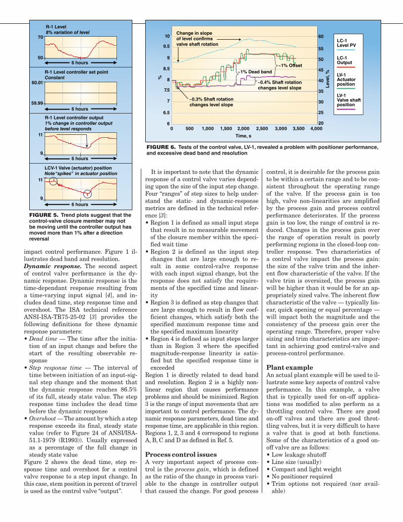
FIGURE 6. Tests of the control valve, LV-1, revealed a problem with positioner performance, and excessive dead band and resolution

• Actuation is usually open or closed with little “positioning” capability

• Less-expensive purchase priceSome of the characteristics of a good throt-tling control valve are as follows:• May have significant leakage when

closed• The body is smaller than line size (usu-

ally)• Valve and accessories require more

space• Valve positioner is usually included • Various trim size and characteristics

available• Actuation has “positioning” capability• More expensive purchase priceIn this plant example, the on-off valve was outfitted with a high-performance, digital valve positioner and “tight fitting” shaft-to-actuator keyways and keys in an effort to provide good throttling performance. The valve was used for level control of a reactor where the level controller output went directly to the control valve posi-tioner as shown in Figure 3. In this pro-cess, it is important to control the level in reactor R-1 to maintain a consistent resi-dence time. It is also important to avoid large changes in the flow from R-1 to R-2 that will upset the R-2 level. The control valve, LV-1, provided tight shutoff as de-sired, but the control performance of the level loop was poor and caused level dis-turbances and unplanned reactor shut-downs. Figure 4 shows the poor perfor-mance of the reactor level control.

One of the first questions that arose in this plant example was whether or not the level controller, LC-1, was properly tuned. The tuning was checked and, although it was not optimum, it was not the source

of the level variations. A closer look at the trends of the LC-1 process variable and output as well as the actuator posi-tion in Figure 5 suggests that the control-valve closure member may not be moving until the controller output has moved more than 1% after a direction reversal. In other words, the control valve had a combined dead band and resolution of ap-proximately 1%, which represents 10% of rate since the valve is operating at about 10% of full travel. Testing the control valve. A special test apparatus was installed on the control valve to measure the rotation of the valve shaft. The valve design was such that the valve closure member, a disc, was solidly attached to the valve shaft and the shaft was large in diameter so that shaft windup should not be significant. Assuming there were no other process disturbances dur-ing the test, the slope of the level process variable can be used to detect a change in the actual flow coefficient of the valve. The response of the actuator position, the valve shaft and the change in flow coeffi-cient can be compared to the input signal. The input signal to the control valve (the output of the controller) was stepped in increments of 0.1% and 0.2% with a re-versal in direction. Figure 6 shows a plot of key variables during the test. The test revealed that the actuator position was “hunting” with about a 0.3% peak-to-peak magnitude. Furthermore, the valve shaft response exhibited a dead band of about 0.8% and a resolution of about 0.2%. Since the control valve was only operating at 8–10% of its capacity, 1% of combined dead band and resolution is a very large non-linearity. And, for a process with an

integrating response, the presence of a dead band will cause a continuous limit cycle in the level and the flow through the valve. In summary, this test revealed a problem with positioner performance and excessive dead band and resolution. The tuning test performed earlier showed that the process gain was excessively high, which amplified the control valve problems. The fact that the valve only op-erated at 8–10% of its capacity indicates that it is oversized, which contributed to the high process gain.The role of control-valve construction. Figure 7 shows details of the construc-tion of the control valve and its actuator. The construction has several characteris-tics that can cause dead band. First, any clearance in the key ways and keys in the coupling will cause dead band. When the valve was initially built, set screws had been used to press into the keys in an at-tempt to reduce slippage between the cou-pling and the shafts. Another source of dead band in this design is the scotch-yoke assembly that converts the linear motion of the actuator to the rotary motion of the actuator shaft. By design, the scotch-yoke assembly must have clearance between the moving parts, but clearance creates dead band [7]. Note that the position of the actuator shaft, not that of the valve shaft, is used for position feedback to the digital valve positioner. Thus, the positioner will measure the position of the actuator shaft and is unaware of the fact that the valve shaft position may differ from the actuator shaft by as much as 1%.

Many of the features of this control-valve construction were appropriate for on-off valve performance, but were in-

Piston actuator Scotch-yoke assembly

converts linear motionto rotary motionActuator shaft

“Keyed” coupling

Valve shaft

Position transmitter (ZT)attached to valve shaftto detect actual valveshaft rotation

Digital valve positioner measures“actuator shaft”position for feedback

Disc

Valve body

Keys

Keyway

Before After

Keyway

Keyway

Keyway

Key

Key

KeyValveshaft

3/8 in.setscrew

Actuator shaft

Coupling

1/2 in.setscrew

1/2 in.setscrew

5/8 in.setscrew

Keyway

Keyway

Keyway

Keyway

Key

Note – Drilled access holes to all 3 setscrews sothat they could be tightened from 0 to 20% position.

Custom key

KeyValveshaft

Actuator shaft

Coupling

FIGURE 7. Many of the features of this control valve con-struction were appropriate for on-off valve performance, but were inherently problematic for throttling performance

FIGURE 8. Improvements were made to the actuator coupling system on the control valve, LV-1

CHEMICAL ENGINEERING WWW.CHE.COM OCTOBER 2010 44

herently problematic for throttling per-formance. In summary, the investigation revealed the following problems with the valve:• Oversized valve creates high process

gain, which amplifies valve non-lineari-ties

• Slack in actuator-to-valve shaft cou-pling, which creates dead band

• Slack in the scotch yoke assembly, which results in dead band

• Poor tuning in digital valve positioner, which results in excessive dead band, resolution and a variation in travel gain

The solution. The recommended solu-tion for this plant example was to replace the control valve with one that is properly sized and has better throttling control performance and sufficient on-off charac-teristics (in this case a tight shut-off). And, the valve positioner should be tuned prop-erly for the optimum response.

In an effort to provide more immediate improvement in the reactor level control, the following interim improvements were made to the control valve: reduce the slack in the actuator coupling system; and im-prove the tuning of the digital valve posi-tioner. To reduce the slack in the actuator coupling system, new keys were machined with a tighter fit in the keyways. Then,

additional and larger set screws were installed in the coupling to press on the keys. Figure 8 shows the changes made to the actuator coupling system. The valve positioner was tuned to provide a faster response time, improve its travel-gain performance and to reduce the tendency to hunt or oscillate.

The interim efforts to improve the con-trol valve performance were beneficial and helped to improve the reactor-level-control performance and reduce the frequency of unplanned reactor trips due to level control disturbances. Figure 9 shows the reactor’s level control performance before and after the interim improvements were made.

The complete recommended solution was to replace the original 18-in. valve with a 12-in. high-performance, segmented-ball, throttling control valve with a spring and diaphragm actuator. This control valve system, similar to the one shown in Figure 10, is specifically designed for throttling applications. A high-perfor-mance, digital valve positioner was in-cluded and was properly tuned to achieve the optimum performance. The new control valve provided even better reac-tor level performance and allowed a 10% production-rate increase and a significant economic benefit. ■

Edited by Dorothy Lozowski

After improvements

Reactorlevel

~ 50% lessvariation invalve positionand flow to downstreamreactor

Before improvements

~ 120 days

FIGURE 9. The reactor level control improved with interim control-valve improve-ments

FIGURE 10. A high-performance,

segmented-ball control-valve system, similar to

the one pictured here, provided better level

performance

AuthorJames Beall is a principal process control consultant at Emerson Process Manage-ment (12301 Research Blvd., Research Park Plaza, Bldg. III, Austin, TX, 78759; Phone: 903–235–7935; Email: James.Beall@Emerson.com) with 29 years of experience in process control. His areas of expertise include process instrumenta-tion, control strategy analysis

and design, control optimization, control valve performance and advanced process control.

References1. Tolliver, Terry, Process Analysis for Improved

Operation and Control, Fisher-Rosemount Systems Advanced Control Seminar, 1996.

2. Bialkowski, W. L., Dreams Versus Reality, A View From Both Sides of the Gap, Keynote Address, Control Systems ’92, Whistler, British Columbia, 1992, published Pulp Pap. Can. 94(11), 1993.

3. ANSI-ISA-TR75-25-02-2000 Control Valve Response Measurement from Step Inputs

4. ANSI-ISA-75-25-01-2000 Test Procedure for Control Valve Response Measurement from Step Inputs.

5. EnTech Control Valve Dynamic Specification V3.0.6. ANSI/ISA 51.1-1979 (R1993) Process Instru-

mentation Terminology.7. Fitzgerald, Bill, “Control Valves for the Chemical

Process Industries”, McGraw-Hill, New York, 1995.

Fisher Controls International

Posted with permission from Chemical Engineering. Copyright © 2010. All rights reserved.#1-28240289 Managed by The YGS Group, 717.505.9701. For more information visit www.theYGSgroup.com/reprints.

Feature ReportALIGN FLUSH LEFT & RIGHT TO PAGE MARGIN

( width may vary )

ASPECT RATIO & GUIDELINES

The FISHER & EMERSON logos should always be scaled proportionally as shown. Logos should not be distorted or stretched.

Align horizontally flush left & right to page margin for Article Reprint.

IF QUESTIONS CONTACT:

Cheryl ClarkFisher Graphics Dept.

641-754-2760

LETTER HEIGHT & ALIGNMENT

CMYK VECTOR ART FOR PRINTING(at page bottom)

ALIGN FLUSH LEFT & RIGHT TO PAGE MARGIN( distance between logos may vary, adjust as appropriate )

gray box indicates width of article contentwidth may vary

appropriate logo placement illustrated below

MARKETING SIGNATURECMYK VECTOR ART & GUIDELINES FOR PRINTING