Improving Bandwidth Estimation for Internet Links by

Improving Bandwidth Estimation for Internet Links by Statistical Methods

Kazumine Matoba, Shingo Ata, and Masayuki Murata

Department of Informatics and Mathematical ScienceGraduate School of Engineering Science, Osaka University1-3, Machikaneyama, Toyonaka, Osaka 560-8531, Japan

Phone: +81-6-6850-6616, Fax: +81-6-6850-6589E-mail: {k-matoba, ata, murata}@ics.es.osaka-u.ac.jp

Abstract Network dimensioning is an important issue to provide stable and QoS–rich communication services.A reliable estimation of bandwidths of links between the end–to–end path is a first step towards the networkdimensioning.Pathchar is one of such tools for the bandwidth estimation for every link between two end hosts.However,pathchar still has several problems. If unexpectedly large errors are included or if route alternationis present during the measurement, the obtained estimation is much far from the correct one. We investigate themethod to eliminate those errors in estimating the bandwidth. To increase the reliability on the estimation, theconfidence interval for the estimated bandwidth is important. For this purpose, two approaches, parametric andnonparametric approaches, are investigated to add the confidence intervals. Another important issue is the methodfor controlling the measurement period. If the link is stable, only a few measurement data is sufficient. On the otherhand, if the data is not sufficient, many measurements is necessary to obtain an accurate and reliable estimation.We propose an measurement method to adaptively control the number of measurement data sets.

1 Introduction

Network dimensioning is becoming a more and moreimportant issue of the day in the Internet. Stable andQoS–rich communication services cannot be providedunless the network is properly dimensioned. One typi-cal example can be found in a diff–serv architecture [1]where the bandwidth should be adequately preparedfor QoS classes. Another example is MPLS [2] andIP–over–WDM networks where the underlying net-work (ATM, SONET or WDM networks) providesphysical paths to connect IP routers. In such a net-work architecture, the physical path capacity shouldbe determined a priori. For ISP to be commerciallysuccessful, QoS provided by ISP is one of importantmeasures in a competitive market.

However, it is not an easy task to dimension the net-work capacity in the Internet since it is quite differentfrom traditional telephone networks. In the telephonenetwork, a historical experience on estimation of calldemand (in erlang) and an Erlang loss formula can beused for that purpose. The traffic estimation is alsonot difficult because the number of blocked calls is ofprimary concern for performance monitoring. Then itcan be used for capacity planning of the links in op-erational networks. We should also note that the Er-

lang loss formula is robust in the sense that it does notrequire the information on the distribution of servicetimes (connection holding times), but only the aver-age. On the other hand, in the Internet offering datacommunication service, such an approach cannot beadopted since it is difficult to know or to estimate thetraffic demand in advance mainly due to the follow-ing two reasons. The one is that the Internet is grow-ing drastically and therefore it cannot forecast futuredemands of user traffic. The other is owing to thecharacteristics of the Internet traffic. The situation isvery different from telephone traffic, which is char-acterized by arrival rates of calls and holding times.A dominant of the Internet traffic is TCP–based ap-plication having a capability of adapting to networkcongestion; i.e., if the network falls into congestion,it defers transmission such that TCP connection is notblocked. Thus, the packet-level metrics of, e.g., thetransfer time and/or loss probability of TCP packetsare not sufficient to identify the performance providedby the operating network. It suggests that the networkmonitoring only at the node and/or link is not sufficientfor capacity planning.

Probably, network dimensioning for the loosely–coupled network just like the Internet needs a differ-ent approach from the conventional telephone network

1

where the network carrier has a responsibility of main-taining the network. Instead, network dimensioningshould be performed in an end–to–end fashion, whichis an essential philosophy of the Internet. Accordingly,various tools have been developed to measure the traf-fic characteristics on the Internet. See, e.g., [3].

An accurate and reliable estimation of the band-width of links on the end–to–end path is a first step to-wards network dimensioning.Pathchar [4, 5] is oneof such tools to measure latency, bandwidth, queue-ing delays and packet loss rate for every link betweentwo hosts. The advantage ofpathchar is that it isnot necessary to deploy new protocols with any specialfunctions at both of routers and end hosts.Pathcharcollects RTTs (Round Trip Time) with various sizes ofpackets and estimates the link bandwidth according tothe relation of RTTs and packet sizes.

However,pathchar still has several problems aswe will explain in detail in Section 2. In short,pathchar needs a large amount of statistics, whichis obtained by throwing the large number of packetsinto the network, to improve the bandwidth estima-tion. However, it has an intrinsic problem that the in-creased traffic may cause congestion and an estimatedvalue is biased bypathchar itself. Instead of pursu-ing the accuracy of the approach taken bypathchar ,we take another approach to add a confidence in theestimation. A recent version ofpatchar , which isnow calledpchar , gives a confidence interval for theslope (by which the bandwidth estimation is derived),but it is insufficient for the user to rely on the obtainedresults. In this paper, we investigate the calculationmethod to determine the confidence intervals for theestimated bandwidth. The control method for mea-surement time is also proposed to limit the unneces-sary probes injected into the network.

The rest of this paper is organized as follows. Sec-tion 2 briefly introducespathchar and point out sev-eral problems that we want to resolve. In Section 3, wepropose our estimation method of the link bandwidthswith confidence intervals. In Section 4, experimen-tal results of our measurement method are shown. Weconclude our paper with future research topics in Sec-tion 5.

2 A Brief Description on Pathcharand its Problems

2.1 A Brief Description on Pathchar

In this subsection, we summarize a bandwidth estima-tion method taken inpathchar . For more details,refer to [4].

0

5

10

15

20

25

30

35

40

45

50

0 200 400 600 800 1000 1200 1400 1600

Rou

nd T

rip T

ime

(ms)

Packet Size (byte)

Figure 1: Distribution of RTT Values vs. Packet Size

Pathchar first collects RTTs between source anddestination hosts. To measure RTTs,pathchar usesone of the ICMP packet, called aTTL expiredmessage,which is also used in traceroute [6]. An IP packet hasa TTL (Time To Live) field in the header. It shows thelimit of the hop count that the packet can traverse. Be-fore the router forwards the packet to the next hop, thevalue of the TTL field is decreased. When the TTLvalue becomes zero, the router discards the packet andreturns the ICMP control packet to the source to informthat the validity of the packet is expired. This mecha-nism is necessary in order to avoid the loops of packetforwarding due to, e.g, some misbehavior of the router.When the packet is sent with the value of the TTL fieldn, the ICMP control packet must be returned fromn thhop router. The RTT value between the source andn throuter on the path can then be measured by the source.Pathchar collects RTTs between the source and ev-ery intermediate router by changing the value of theTTL field.

The measured RTT value consists of (1) the sum ofqueueing delays,qi, at routeri (1 ≤ i ≤ n), (2) thesum of transmission times to transmit the packet by theintermediate routers, (3) the sum of forwarding timesfi that routeri processes the packet, and (4)the sum ofpropagation delayspj of link j (1 ≤ j ≤ n). Thatis, RTTs, the RTT value for given packet sizes, isrepresented by

RTTs =n∑

j=1

(s

bj+

sICMP

bj

)+

n∑i=1

(qi+fi)+2n∑

j=1

pj.(1)

wheresICMP is a size of an ICMP error message andbj is the bandwidth of linkj.

A typical example for the relation between packetsizes and measured RTTs is shown in Figure 1. Theresults are obtained by setting the destination to bewww.gulf.or.jp from our site. The TTL valuewas set to 16. It was obtained on Dec 18 12:54 JST.The figure shows that the RTT values were widely

2

spread even for the fixed packet size. It is because thequeueing delay at the router changes frequently by thenetwork condition. However, it is likely that severalpackets do not experience the queueing delays at anyrouter by increasing the trials. Such a case actually ap-pear in the figure as a minimum value of RTTs for eachpacket size. The minimum RTT for given packet sizes, denoted byminRTTs, is thus obtained by

minRTTs =n∑

j=1

s + sICMP

bj+

n∑i=1

fi + 2n∑

j=1

pj . (2)

Note that the packet size of the ICMP error messagesICMP is fixed (56 bytes). Then, by collecting termsnot related to the packet size and denoting it byα, theabove equation can be rewritten as

minRTTs = sn∑

j=1

1bj

+ α. (3)

The above equation is a linear equation with respect tothe packet sizes. It is just shown in Figure 1 if we lookat the minimum RTT values. By letting the coefficientof the above equation beβn, we have

βn =n∑

j=1

1bj

. (4)

Conversely, if we haveβn−1 andβn, we can obtain thebandwidth of linkj as

bj =1

βn − βn−1. (5)

It is a key idea ofpathchar .As indicated above, a difficulty ofpathchar ex-

ists in that in real networks such as the Internet, net-work conditions change frequently, and it is not easyto obtain proper minimum RTTs. Thus,pathcharneeds to send many packets with the same size; it is aweak point ofpathchar since those waste a largeamount of link bandwidth to get a minimum RTT.Even after many RTTs are collected, some measure-ment errors must be contained.Pathchar solves thisproblem by a linear least square approximation.

2.2 Problems ofPathchar

The approach of the bandwidth estimation taken bypathchar is innovative, but it still has several prob-lems as we describe below.

2.2.1 Reliability on Obtained Estimation

First, we cannot know whether the estimated band-width obtained bypathchar is reliable or not. There

is no way to have a confidence on the accuracy of theestimated value inpathchar . Pathchar uses thelinear least square fitting to calculateβn, which meansthat it assumes errors of minimum RTTs are normallydistributed [4]. However, we have no means to con-firm whether errors follow a normal distribution ornot. From this reason, it is necessary to consider an-other approach that can lead to bandwidth estimationindependently of the error distribution. Such an ap-proach is often called as a nonparametric approach.The nonparametric approach is already developed inpchar [7], an updated version ofpathchar . Whilein pchar , the user can choose the parametric or thenonparametric method for estimation, it does not offerany criterion to decide which approach is better.

2.2.2 Efficiency of Measurements

The second problem is the efficiency ofpathchar .Pathchar sends a fixed number of packets, but theamount of collected data must be changed accordingto the network condition to measure the link band-width within a reasonable level of accuracy. The au-thors in [4] then propose anadaptivedata collectionmethod to improve the efficiency ofpathchar . Theyhave shown that the required number of packets inpathchar can much be reduced ifpathchar isequipped with an ability to send a different number ofpackets for each link estimation. In their proposal, thenumber of transmitted packets is decided by observingwhether the even-odd range of bandwidth is convergedor not. However, the range is not based on the reliabil-ity on the result and the method does not guarantee anaccuracy in astatisticalsense.

2.2.3 Exceptional Errors of RTTs

The third problem is that various kinds of errors aremixedly contained in minimum values of RTT. Never-theless,pathchar assumes that the error of the min-imum RTT is originated from the measurement noiseonly, and therefore assumes the normal distributionfor measurement errors. Basically,pathchar relieson the fact that the queueing delay at the intermedi-ate routers can be removed by gathering a number ofmeasurements since one or more packets must fortu-nately encounter no queueing delay by increasing themeasurement. If the number of measurements is insuf-ficient, the queueing delay may be involved, but it maybe able to be viewed as a Gaussian noise.

The problem is that we encounter the errors whichcannot be explained by the Gaussian noise. Oneexample is shown in Figure 2, which was obtainedat Dec 21 08:39 JST by setting the destination as

3

0

5

10

15

20

25

30

35

40

45

50

0 200 400 600 800 1000 1200 1400 1600

Rou

nd T

rip T

ime

(ms)

Packet Size (byte)

Figure 2: A Sample of Errors Not Following a NormalDistribution

www.try-net.or.jp and the TTL value as 13.Several small values were observed during the mea-surement as shown in Figure 2. We need to introducesome method to remove such errors before the band-width estimation is performed. For this purpose, weuse a weighted least square fitting method as will beexplained in Subsection 3.1.

A second example was obtained by route alterna-tion. To get the bandwidth estimation, all probesshould be relayed on the same path. Ifpathchardetects the route changes by checking the field of thesource IP address in the returned ICMP packet, it sim-ply discards the returned packet. Such a case mayhappen due to load balancing at routers [8]. Theproblem is that it cannot eliminate the case wherethe source IP addresses of the returned ICMP pack-ets are same, but the relayed paths are different. Infact, we obtained such measurement as shown in Fig-ure 3. It was observed at 8-th link destined forwww.kyotoinet.or.jp at Dec 10 12:29 JST).Figure 3 clearly shows that there exist two (or maybemore) paths during the measurement. To remove suchan effect, we need to select the proper subgroup ofRTTs for accurate estimation, which will be explainedin Subsection 3.2

3 Accuracy and Reliability Improve-ments for Bandwidth Estimation

As we have discussed in the previous section, we needto solve several problems for obtaining accurate andreliable bandwidth estimation. For this purpose, wefirst examine two estimation methods; parametric andnonparametric approaches to obtain the accurate re-sult. The approach to obtain the confidence interval isalso described to increase the reliability on estimation.Those are presented in Subsection 3.1. Our cluster-

0

5

10

15

20

25

30

35

40

45

50

0 200 400 600 800 1000 1200 1400 1600

Rou

nd T

rip T

ime

(ms)

Packet Size (byte)

Figure 3: A Sample having Two Groups of RTTs

ing method to pick up proper RTTs from two or moregroups of RTTs is then presented in Subsection 3.2.An adaptive mechanism to control the measurementperiod is finally described in Subsection 3.3. Our ex-perimental results based on those methods are shownin the next section.

3.1 Accurate and Reliable Slope EstimationMethods

As having been described in the previous sec-tion, using the linear least square fitting method inpathchar implies that errors follow a normal dis-tribution. Thus, unexpectedly large errors (as shownin Figure 2 significantly affect the accuracy of the es-timated value. To eliminate such an influence, we in-troduce two estimation methods instead of the linearleast square fitting method. One is an M–estimationmethod with a Tukey’s biweight function [9], which isa sort of the parametric approach. It is a robust esti-mation method to produce results with uniformly highefficiency. Because it presumes that almost all datais reliable and only some data includes unexpectedlylarge errors, the result is robust even if the large errorsare contained as in our case. The other is a nonpara-metric linear least square fitting method which doesnot assume any distribution on measurement errors. Inwhat follows, we will describe two methods in turn.

3.1.1 M–estimation Method

In this subsection, we describe the weighted leastsquare fitting method. With this method, the influenceof the large error can be limited. Note that this methodis applicable only when the number of large errors isnot large. Otherwise, we need to use a nonparametricapproach which is independent of an error distribution.The latter approach is presented in the next subsection.

The M–estimation method is an extension of a4

Figure 4: The Biweight Function

maximum likelihood estimation method. In the M–estimation method, the weighted least square fitting isiterated to calculate an appropriate weight. There aresome variations in the M–estimation method, and weapply the Turkey’s biweight function which is consid-ered to be one of the best estimation methods. In theTukey’s biweight function, a weight function is chosenas shown in Figure 4. It is apparent from the figure thatthe Tukey’s biweight function is robust against the un-expectedly large errors if those occur infrequently. Letthe number of kinds of the packet size bem. After wecollect a minimum value of RTT for each packet size,we can estimate the slope according to the followingprocedure. Note that the slope means a coefficientβn

for routern (see Eq. (4)). In the following equations,we omitn for brevity.

1. The straight line is expressed byy = α + βx,wherex is a packet size andy is an ideal mini-mum RTT. We set initial values of a vertical inter-ceptα and a slopeβ with the least square fittingmethod;

β =∑m

i=1 xiyi − mxy∑mi=1 xi

2 − mx2, (6)

α = y − βx, (7)

wherex andy shows the mean ofxi andyi.

2. Calculate the difference|vi| between the mini-mum RTT and the point on the straight line, i.e.,

|vi| = |yi − y|. (8)

3. By obtaining the median of differences, the stan-dard size of an errors is calculated as

s = median{|vi|}. (9)

4. Using the biweight function, we set a weight ad-justment factorωadj

i for each difference;

ωiadj =

{ [1 − ( vi

c s)2]2 if |vi| < c s,

0 otherwise(10)

wherec is a constant value used as an index formaking the total weight to be zero.

5. Let ωi denote the weight of RTTs, which is de-fined by

ωi =mωi

adj∑mi=1 ωi

adj. (11)

We then estimate new values ofα andβ with theweighted least square fitting.

α =∑m

i=1 ωi yi

m, (12)

β =∑m

i=1 ωi xi yi∑mi=1 ωi x2

i

. (13)

6. After k iterations, we adoptα andβ as solutions.

The parameterc in Eq. (10) controls a boundary forthe errors contained in measured RTT values to beneglected. Through our experiments, we found thatc = 3 and the number of iterationsk = 5 are suffi-cient. Note that slopes of straight lines are always con-verged in our experimental results when we use aboveparameter values.

We introduce the following assumptions to calculatea confidence interval with the M-estimation method.

• For given packet sizex, the random variable ofthe minimum RTT,Y follows the normal distri-bution, whose mean and variance are given byα + βx andσ2, respectively.

• The numberm of measurements for each packetsize are mutually independent.

The above assumptions imply that the set of sloes fol-lows the normal distribution with meanβ and varianceσ2

B . We obtain these parameters by

β =∑m

j=1(xj − x)(Yj − Y )∑mj=1(xj − x)2

, (14)

σ2B =

σ2∑mj=1(xj − x)2

, (15)

whereσ2 is the variance of the RTTs from the estimateline. It can be estimated from the measurement data as

σ2 =1m

m∑j=1

(yj − α − βxj)2. (16)

From Eq. (14), we can calculate the values of the slopefor links n − 1 and n as βn−1 and βn, respectively.

5

The variances for linkn − 1 andn are also estimatedasσ2

n−1 andσ2n from Eq. (15).

Once those values are given, we next calculate theconfidence interval as follows. We can estimate themean and variance for the difference of slopes as

βu = βn − βn−1, (17)

σ2u = σ2

n − σ2n−1. (18)

1/βu just gives an bandwidth estimation for linkn.Results must followt-distribution withm − 2 degreesof freedom. Thus, we first obtain the intervalk as

k =c σu√m − 2

, (19)

wherec is a 97.5% value of thet–distribution if wewant 95% confidence interval. Then we have the con-fidence interval for the estimated bandwidth1/βu as

1/(βu + k) ≤ 1/βu ≤ 1/(βu − k). (20)

Then, we have a reliable estimation by adding theconfidence intervals. However, it is assumed that mea-surement errors follow the normal distribution after thevery large errors are excluded by the biweight func-tion. In the next subsection, we will present a non-parametric estimation method which does not requireany assumption on the error distribution.

3.1.2 Nonparametric Estimation Method

In the nonparametric approach, we do not need any as-sumption on the error distribution. Letm be the num-ber of obtained measurement data set for each packetsize as before. The slope estimation can be obtainedby the following procedure.

1. By choosing the every combination of two min-imum values of RTTs, and calculate the slope.That is, we havem(m− 1)/2 slopes by this step.

2. We sort a set of obtained slopes and adopt its me-dian as the proper slope.

A Kendall’s τ method [10] is known as a way offinding the confidence interval in the nonparametricmethod. However, it cannot be directly applied tothe current problem since it is necessary to calculatethe difference of two slopes. Alternatively, we use aWilcoxon’s method [11], which is based on the differ-ence between medians of two data setsSandT.

In the current context, we use two sets of slopes ob-tained from the measurements for linksn − 1 andn,which are denoted asS andT, respectively. By lettingthe numbers of elements ofS and T be |S| and |T |,

respectively, we label elements of two setsS andT ass(j) andt(i) (1 ≤ i ≤ |T |, 1 ≤ j ≤ |S|). The band-width estimation and its confidence interval is then ob-tained as follows.

1. Calculate the set of differencesT (i)− S(j) (1 ≤i ≤ |T |, 1 ≤ j ≤ |S|). Let us denote the obtainedset of the differences asU.

2. Sort the setU.

3. Letu(i)(1 ≤ i ≤ |S|×|T |) denoteith element ofsorted setU. The confidence interval is then givenby

u

( |T |(2|S |+ |T |+ 1)2

+ 1 − a

)≤ βu

≤ u

(a − |T |(|T |+ 1)

2

). (21)

If we want 95% confidence interval, parametera should be determined such that the probabilityP (∑

u(i) ≥ a) is equal to0.975. When the num-bers of measured data|S| and |T | are large, it isknown that

∑u(i) follows the normal distribu-

tion with mean|T |(|S |+ |T |+1)/2 and variance|S||T |(|S |+ |T |+ 1)/12. Thus, we can approxi-matea as;

a =|T |(|S |+ |T |+ 1)

2+

12

+ 1.96

√|S||T |(|S |+ |T | + 1)

12. (22)

However, we have a problem in the above proce-dure. Our goal is to control the measurement timeso that the measurement is finished when the confi-dence interval of the bandwidth estimation is withina prespecified value. For that purpose, on–line cal-culation is necessary. However, the above procedurerequires much computational time. Suppose that wegather RTT values with 45 kinds of packet sizes as inpathchar . The number of slopes obtained for eachlink becomes 990, and therefore the number of ele-ments ofU is about 1,000,000. It is too large for themethod described above.

We therefore use another method based on aKendall’s rank correlation coefficient [10]. We obtainm(m − 1)/2 slopes fromm trials for each link, andtherefore the number of elements|S| and|T | becomesm(m−1)/2. We therefore use the following procedureto estimate the cofidence intervals.

1. SortS andT, and obtain the setU’ , the elementof which is calculated byu′(i) = s(i)− t(i) (1 ≤i ≤ m(m − 1)/2).

6

2. The confidence interval ofU’ is then determinedby the following equation.

u′(

m(m−1)2 − C

2

)≤ βu′ ≤ u′

(m(m−1)

2 + C

2

),(23)

whereC is the Kendall’s rank correlation coeffi-cient. IfK is 97.5% value of the standard normaldistribution andn is enough large, we obtain 95%confidence interval by using

C = K

√m(m − 1)(2m − 5)

18. (24)

The on–line calculation procedure and stopping rulefor the RTT measurement will be described in Subsec-tion 3.3.

3.2 Removal of Unnecessary RTT Values

As having been shown in Figure 3, it is necessary topick up proper RTTs when the distribution of RTT con-sists of several groups of RTTs. It is caused by routealternation thatpathchar can never detects. To di-vide data into several groups, we use the clusteringmethod [12]. After we obtain the measurement data,we first abondone the upper 30% of measured RTTssince those does not help estimating the link band-width. Then, we divide them into several clusters.

We assume that the cluster having the largest num-ber of measured elements contains the actual minimumRTT. If route alternation does not occur during themeasurement, it is not necessary to apply the cluster-ing. We can know it if divided clusters are very closewith each other. Figure 5 plots the result of the cluster-ing using the data shown in Figure 3. Note that we di-vided the gathered data into three clusters. The figureshows that we can extract the clusters of RTTs prop-erly. A weak point of this procedure is that it takesmuch time for clustering and therefore we cannot re-peat clustering for every packet arrival. From this rea-son, we perform clustering after the measurement ofRTTs is finished.

3.3 An Adaptive Mechanism to Control theMeasurement Period

We finally describe our bandwidth estimation method.Our method can control the measurement period sothat the measurement terminates when the prescribedconfidence intervals are satisfied. During the measure-ment, inacurate data is dropped as described in the pre-vious subsection. Then, one can rely on the obtaineddata with confidence intervals.

0

5

10

15

20

25

30

35

40

45

50

0 200 400 600 800 1000 1200 1400 1600

Rou

nd T

rip T

ime

(ms)

Packet Size (byte)

Figure 5: Result of Clustering

More specifically, the following procedure is per-formed during the RTT measurement. In describingthe procedure below, we suppose that the bandwidthestimation for link(n − 1) has already been finished.

1. For estimating the bandwidth of linkn, we firstsend a fixed number of packets. For example,we send 10 packets in our experiments presentedin the next section. Then, RTTs are collectedfor 46 kinds of the packet size (from 40 bytes to1,500 bytes). Namely, the source sends10×46 =460 packets for the initial measurement.

2. For taking account of route alternation, we checkthe source address of the ICMP packets as inpathchar . We take routern, the address ofwhich appears most in the ICMP packets.

3. We then estimate the initial bandwidth and itsconfidence interval ofn th link by our estimationmethods (see Subsection 3.1).

4. To get the accurate bandwidth estimation andconfidence interval, we iterate following proce-dures.

(a) We send an additional set of probes (e.g.,10 packets for each packet size) to get newRTTs for routern.

(b) For each RTT, we check whether the mea-sured RTT is smaller than the minimumRTT. If so, we calculate the new values ofthe difference of measured RTT and the onederived from the estimated slope, and com-pare the new difference with the originalone. If the difference is much smaller thanthe original difference, we replace the mini-mum value of RTT with the new RTT value.In the experiment presented in the next sec-tion, we abondone the new data if it is largerthan 30% of the previous difference.

7

(c) To keep the number of samples for each linkto be identical, we send additional packetsto router(n−1) when the source sends morepackets to routern.

(d) By using our estimation approach (theparametric approach described in Subsec-tion 3.1.1 or the nonparametric approach inSubsection 3.1.2), we update the bandwidthestimation and its confidential interval. Theiteration is finished if the confidence inter-val of the estimated bandwidth becomes lessthan the prescribed value.

5. After the iteration terminates, we finally verifywhether RTTs have reasonable values. A mostimportant task at this step is to apply the cluster-ing technique. If RTTs are not proper because ofroute alternation, we retry the measurement pro-cess by returning to Step 4.

4 Experimental Results and Discus-sions

4.1 Removing Irregular RTT Values due toExceptionally Large Errors

We first show experimental results for the case whereRTT values apparently do not follow the normal distri-bution because of some large errors. The example wasshown in Figure 2. Figure 6 plots only minimum val-ues of RTTs against the packet size from Figure 2. Asshown in this figure, the variation of minimum RTTsexhibits far from the linear relation. Figure 7 com-pares results of the slope estimations bypathchar ,pchar , and our methods (the M-estimation and non-parametric methods). Straight lines ofpathchar andpchar are inaccurate due to exceptionally large errorswhose packet sizes are 288, 960, 1376, and 1440 bytes.On the other hand, our approach can filter out such er-rors.

Table 1 shows the estimated values. In the figure,two cases of the bandwidth estimation are shown; 13-th link from 202.231.198.2 destined for 210.142.124.1(corresponding to Figure 2) and 13-th link from202.232.8.66 destined for 210.141.224.162. The ca-pacities of those links were known a priori as 1.5 Mbpsand 45 Mbps. For each of two links, we show the es-timated bandwidth obtained by all methods. Addition-ally, confidence intervals of 95% are also shown in ourmethods. As shown in the table, results obtained bypathchar andpchar are far from the actual band-width, while our methods can give very close values.

0

5

10

15

20

25

30

35

0 200 400 600 800 1000 1200 1400 1600

Rou

nd T

rip T

ime

(ms)

Packet Size (byte)

Figure 6: Minimum values of RTTs including irregularvalues

0

5

10

15

20

25

30

35

0 200 400 600 800 1000 1200 1400 1600

Rou

nd T

rip T

ime

(ms)

Packet Size (byte)

pathchar,pchar

M-estimationnonparametric

Figure 7: Estimated lines for the case with irregularvalues

The difference of the actual bandwidth and the esti-mated bandwidth is due to the overhead of the under-lying network. In the case of 45 Mbps link, our meth-ods seem to offer very accurate estimation. Perhaps, itis not true since we must take account of the overheadof the underlying network.

In the table, the numbers of packets transmitted foreach packet size are also shown. In our methods, thevery small number of packets were sufficient to obtainthe accurate results for 1.5 Mbps link. For 45 Mbpslink, on the other hand, 200 packets were necessary,which is same aspathchar . It is due to the factthat as the link bandwidth becomes large, the accurateestimation becomes difficult, which has already beenpointed out by [4].

In the case of 1.5 Mbps link, we cannot observe dif-ferences among our three methods, the M-estimation,Wilcoxon’s and Kendall’s methods. In the case of45 Mbps link, the M-estimation method seems to bebest. However we cannot decide the best one here be-cause we found many cases that the other method givesthe best result, as will be presented in the below.

8

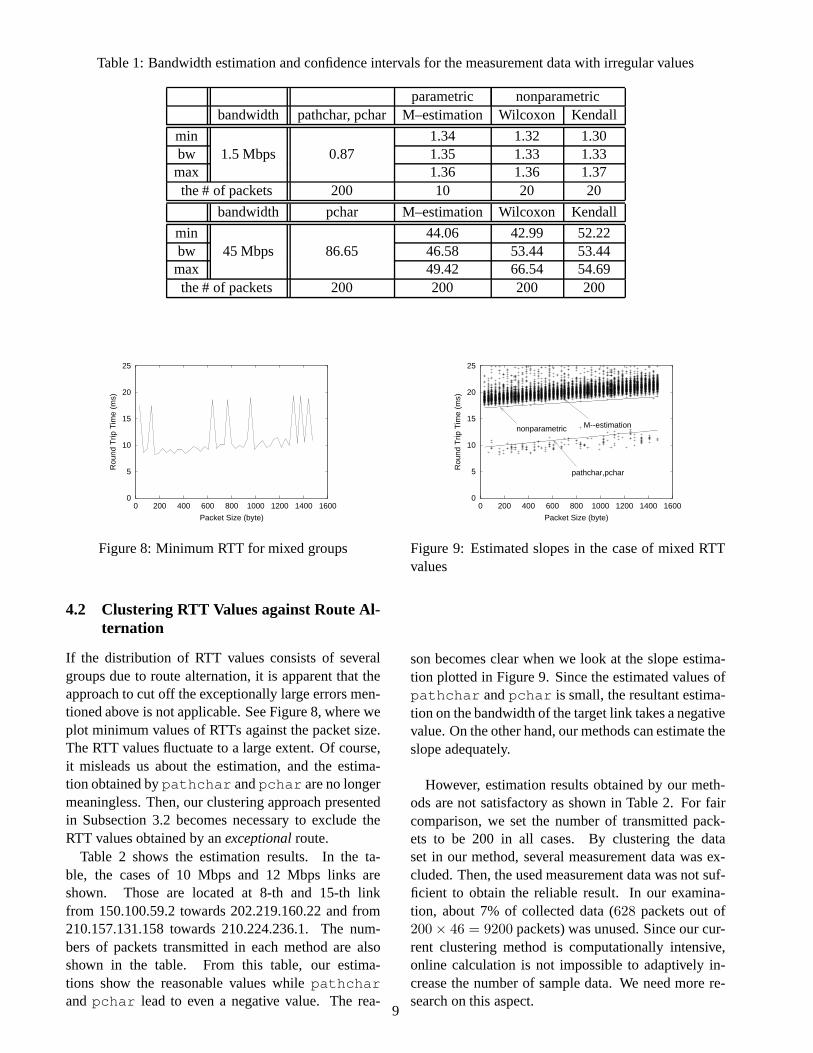
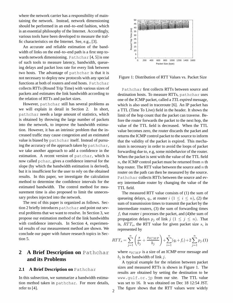
Table 1: Bandwidth estimation and confidence intervals for the measurement data with irregular values

parametric nonparametricbandwidth pathchar, pchar M–estimation Wilcoxon Kendall

min 1.34 1.32 1.30bw 1.5 Mbps 0.87 1.35 1.33 1.33max 1.36 1.36 1.37the # of packets 200 10 20 20

bandwidth pchar M–estimation Wilcoxon Kendall

min 44.06 42.99 52.22bw 45 Mbps 86.65 46.58 53.44 53.44max 49.42 66.54 54.69the # of packets 200 200 200 200

0

5

10

15

20

25

0 200 400 600 800 1000 1200 1400 1600

Rou

nd T

rip T

ime

(ms)

Packet Size (byte)

Figure 8: Minimum RTT for mixed groups

4.2 Clustering RTT Values against Route Al-ternation

If the distribution of RTT values consists of severalgroups due to route alternation, it is apparent that theapproach to cut off the exceptionally large errors men-tioned above is not applicable. See Figure 8, where weplot minimum values of RTTs against the packet size.The RTT values fluctuate to a large extent. Of course,it misleads us about the estimation, and the estima-tion obtained bypathchar andpchar are no longermeaningless. Then, our clustering approach presentedin Subsection 3.2 becomes necessary to exclude theRTT values obtained by anexceptionalroute.

Table 2 shows the estimation results. In the ta-ble, the cases of 10 Mbps and 12 Mbps links areshown. Those are located at 8-th and 15-th linkfrom 150.100.59.2 towards 202.219.160.22 and from210.157.131.158 towards 210.224.236.1. The num-bers of packets transmitted in each method are alsoshown in the table. From this table, our estima-tions show the reasonable values whilepathcharandpchar lead to even a negative value. The rea-

0

5

10

15

20

25

0 200 400 600 800 1000 1200 1400 1600

Rou

nd T

rip T

ime

(ms)

Packet Size (byte)

M--estimation

pathchar,pchar

nonparametric

Figure 9: Estimated slopes in the case of mixed RTTvalues

son becomes clear when we look at the slope estima-tion plotted in Figure 9. Since the estimated values ofpathchar andpchar is small, the resultant estima-tion on the bandwidth of the target link takes a negativevalue. On the other hand, our methods can estimate theslope adequately.

However, estimation results obtained by our meth-ods are not satisfactory as shown in Table 2. For faircomparison, we set the number of transmitted pack-ets to be 200 in all cases. By clustering the dataset in our method, several measurement data was ex-cluded. Then, the used measurement data was not suf-ficient to obtain the reliable result. In our examina-tion, about 7% of collected data (628 packets out of200 × 46 = 9200 packets) was unused. Since our cur-rent clustering method is computationally intensive,online calculation is not impossible to adaptively in-crease the number of sample data. We need more re-search on this aspect.

9

Table 2: Bandwidth estimation and confidence intervals for the case of mixed RTTs

parametric nonparametricbandwidth pathchar,pchar M–estimation Wilcoxon Kendall

min 10.07 16.59 14.24bw 10 Mbps -22.6 12.40 16.95 16.95max 16.11 24.07 25.29the # of packets 200 200 200 200


34

36

38

40

42

44

0 200 400 600 800 1000 1200 1400 1600

Rou

nd T

rip T

ime

(ms)

Packet Size (byte)

M--estimation

pathchar,pchar

nonparametric

Figure 10: RTT values and estimated slopes

4.3 Controlling the Measurement PeriodAdaptively

We next show how our adaptive control of the mea-surement period works. Different from previous cases,we pick up the cases wherepathchar can also showthe reasonable results in this subsection. Figure 10compares estimated slopes of minimum RTTs amongpathchar , pchar and our methods. As shown inthe figure, there is no remarkable difference among allestimation methods. Table 3 also shows the same ten-dency; estimated values of link bandwidths are quiteclose with each other. These results suggest that theerror contained in the minimum values of RTT can bemodeled by a normal distribution in usual cases if theamount of measurement data is sufficiently large.

However, our estimation approaches have two ad-vantages overpathchar (and pchar ). First, ourmethod can control the number of probes adaptively.As shown in Table 3, the measurement terminates witha less number of probes in our method except the caseof 6 Mbps link. Table 4 summarizes the required num-ber of probes to obtain the 95% confidence intervalswhere minimum and maximum values are within 5%

difference from the mean value. Note that symbol‘*’ in the table shows that the result does not reachwithin the prescribed confidence interval by that num-ber of probes. For several links, the number of probesfor each packet size is less than 200. On the otherhand, the number of transmitted probes bypathcharwas 200; it implies thatpathchar wastes the net-work bandwidth by unnecessarily transmitting pack-ets. For other cases, the numbers of probes are largerthanpathchar , but we can expect that the resultantestimated values become more reliable than the valuesobtained bypathchar .

Between parametric and nonparametric approaches,the required number of probes by the nonparametricapproach is larger than that of the parametric approach.It is natural since the nonparametric approach does notassume any distribution on errors. Then, it needs alarger number of probes for reliable estimation. Thelarge number of probes was necessary for the secondlink in the table in spite of 10 Mbps link. It is becausethe utilization of that link was high. It verifies that ourmethod can adaptively increase the number of probesaccording to the link congestion. A second advantageof our methods is that we can obtain unified degrees ofconfidence on all links. On the other hand, the accu-racy of estimation bypathchar is varied, and moreimportantly, there is no means to know about reliabil-ity on the estimated values.

4.4 Online Estimation of Confidence Inter-vals

We last discuss on the derivation methods of con-fidence intervals in our methods. As having beendescribed in Section 3.1.2, the method based onKendall’s rank correlation coefficient is approximatein obtaining the confidence interval, and it mustbe less accurate than the one based on Wilcoxon’s

10

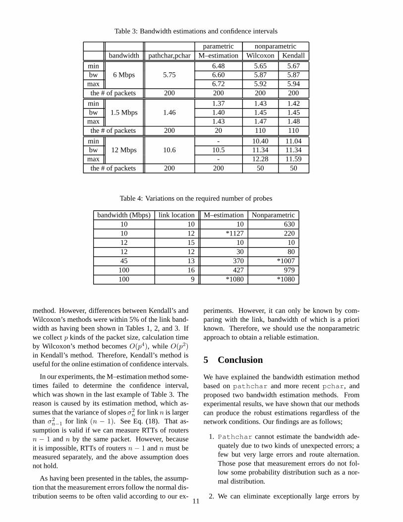
Table 3: Bandwidth estimations and confidence intervals

parametric nonparametricbandwidth pathchar,pchar M–estimation Wilcoxon Kendall


min 1.37 1.43 1.42bw 1.5 Mbps 1.46 1.40 1.45 1.45max 1.43 1.47 1.48the # of packets 200 20 110 110

min - 10.40 11.04bw 12 Mbps 10.6 10.5 11.34 11.34max - 12.28 11.59the # of packets 200 200 50 50

Table 4: Variations on the required number of probes

bandwidth (Mbps) link location M–estimation Nonparametric10 10 10 63010 12 *1127 22012 15 10 1012 12 30 8045 13 370 *1007100 16 427 979100 9 *1080 *1080

method. However, differences between Kendall’s andWilcoxon’s methods were within 5% of the link band-width as having been shown in Tables 1, 2, and 3. Ifwe collectp kinds of the packet size, calculation timeby Wilcoxon’s method becomesO(p4), while O(p2)in Kendall’s method. Therefore, Kendall’s method isuseful for the online estimation of confidence intervals.

In our experiments, the M–estimation method some-times failed to determine the confidence interval,which was shown in the last example of Table 3. Thereason is caused by its estimation method, which as-sumes that the variance of slopesσ2

n for link n is largerthanσ2

n−1 for link (n − 1). See Eq. (18). That as-sumption is valid if we can measure RTTs of routersn − 1 andn by the same packet. However, becauseit is impossible, RTTs of routersn − 1 andn must bemeasured separately, and the above assumption doesnot hold.

As having been presented in the tables, the assump-tion that the measurement errors follow the normal dis-tribution seems to be often valid according to our ex-

periments. However, it can only be known by com-paring with the link, bandwidth of which is a prioriknown. Therefore, we should use the nonparametricapproach to obtain a reliable estimation.

5 Conclusion

We have explained the bandwidth estimation methodbased onpathchar and more recentpchar , andproposed two bandwidth estimation methods. Fromexperimental results, we have shown that our methodscan produce the robust estimations regardless of thenetwork conditions. Our findings are as follows;

1. Pathchar cannot estimate the bandwidth ade-quately due to two kinds of unexpected errors; afew but very large errors and route alternation.Those pose that measurement errors do not fol-low some probability distribution such as a nor-mal distribution.

2. We can eliminate exceptionally large errors by11

utilizing the biweight estimation method, whichis applicable to both of M–estimation and non-parametric least square fitting methods.

3. By clustering the measured RTTs and selectingan appropriate cluster, errors introduced by routealternation can be avoided.

4. By obtaining the confidence interval, a measure-ment period can be controlled, which makes itpossible to reduce the measurement period andavoid bandwidth waste caused by unnecessaryprobes in some cases. If the link is congested, onthe other hand, more probes are transmitted ac-cording to our method. Then accurate and, moreimportantly, reliable estimation becomes possi-ble.

5. Between parametric and nonparametric ap-proaches, the latter is adequate for reliable band-width estimation, but it requires more measure-ment time. The parametric approach (i.e., the M-estimation method) is better in the measurementand computational time. Perhaps, it depends onthe link condition. If the link load is not high, theobtained measurement data is stable. Then, theassumption that the measurement errors followthe normal distribution would hold. Otherwise,the nonparametric approach presented in this pa-per would be necessary. However, its validationremains as a future research topic.

References

[1] S. Blake, D. Black, M. Carlson, E. Davies, Z. Wangm,and W. Weiss, “An architecture for differentiated ser-vices,” IETF RFC 2475, December.

[2] E.C.Rosen, A.V.Than, and R.Callon, “Multiprotocollabel switching architecture,”IETF draft, Mar 1998.

[3] “Caida measurement tool taxonomy,”http://www.caida.org/Tools/taxonomy.html .

[4] A. B. Downey, “Using pathchar to estimate Internetlink characteristics,”Proceedings of ACM SIGCOMM,pp. 241–250, August 1999.

[5] V. Jacobson, “pathchar,”ftp://ftp.ee.lbl.gov/pathchar/ .

[6] V. Jacobson, “traceroute,”ftp://ftp.ee.lbl.gov/traceroute.tar.Z .

[7] B. A. Mah, “pchar: A tool for measuring Internetpath characteristics,”http://www.ca.sandia.gov/˜bmah/Software/pchar .

[8] V. Paxon, “Measurements and analysis of end-to-endinternet dynamics,”Ph.D.Thesis, April 1997.

[9] J.W.Tukey, “Introduction to today’s data analysis,”Proceedings of the Conference on Critical Evalua-tion of Chemical and Physical Structural Information,pp. 3–14, 1974.

[10] M.G.Kendall, “Rank corelation methods,” 1970.

[11] G.Noether, “Some simple distribution–free confi-dencd intervals for the center of a symmetric distri-bution,” J. Am. Statist. Assoc., pp. 716–719, 1973.

[12] J. A. Hartigan,Clustering algorithms. John Wiley &Sons, 1975.

12

Documents

Improving Bandwidth Estimation for Internet Links by