Improving automatic correctionof article errors

Rutger Kraaijer10382259

Bachelor thesisCredits: 18 EC

Bachelor Opleiding Kunstmatige Intelligentie

University of AmsterdamFaculty of ScienceScience Park 904

1098 XH Amsterdam

SupervisorDr. T. Deoskar

Institute for Language, Logic and ComputationFaculty of Science

University of AmsterdamScience Park 107

1098 XG Amsterdam

June 24th, 2016

Abstract

In this thesis possible improvements are evaluated which try to im-prove the automatic correction of article errors (the, a, an) by using aclassification algorithm. Two distinct problems are examined: represent-ing the head noun as a vector, and quantifying information around a nounphrase. This is achieved by using a clustering algorithm on word embed-ding vectors to group similar words to reduce the feature dimensionalityof a head noun representation, and considering the frequency of the headnoun in previous sentences. The clustering method shows a small positiveinfluence on the classifier. The context feature did not show a significantimpact.

1

Contents

1 Introduction 31.1 Words as a feature . . . . . . . . . . . . . . . . . . . . . . . . . . 41.2 Word categories . . . . . . . . . . . . . . . . . . . . . . . . . . . . 41.3 Context . . . . . . . . . . . . . . . . . . . . . . . . . . . . . . . . 51.4 Thesis overview . . . . . . . . . . . . . . . . . . . . . . . . . . . . 5

2 Literature review 62.1 Word categories . . . . . . . . . . . . . . . . . . . . . . . . . . . . 72.2 Context . . . . . . . . . . . . . . . . . . . . . . . . . . . . . . . . 8

3 Methodology 83.1 Analysis of the data . . . . . . . . . . . . . . . . . . . . . . . . . 8

3.1.1 Noun frequencies . . . . . . . . . . . . . . . . . . . . . . . 93.1.2 Baseline . . . . . . . . . . . . . . . . . . . . . . . . . . . . 93.1.3 Cutoffs . . . . . . . . . . . . . . . . . . . . . . . . . . . . 103.1.4 Mass nouns . . . . . . . . . . . . . . . . . . . . . . . . . . 11

3.2 Features . . . . . . . . . . . . . . . . . . . . . . . . . . . . . . . . 113.2.1 Reference . . . . . . . . . . . . . . . . . . . . . . . . . . . 113.2.2 Word categories . . . . . . . . . . . . . . . . . . . . . . . 133.2.3 Context . . . . . . . . . . . . . . . . . . . . . . . . . . . . 13

3.3 Pre-processing . . . . . . . . . . . . . . . . . . . . . . . . . . . . 133.3.1 Extracting from corpus . . . . . . . . . . . . . . . . . . . 143.3.2 Tagging . . . . . . . . . . . . . . . . . . . . . . . . . . . . 153.3.3 Parsing . . . . . . . . . . . . . . . . . . . . . . . . . . . . 153.3.4 Frequency analysis . . . . . . . . . . . . . . . . . . . . . . 173.3.5 Clustering . . . . . . . . . . . . . . . . . . . . . . . . . . . 173.3.6 Feature creation . . . . . . . . . . . . . . . . . . . . . . . 17

3.4 Machine learning . . . . . . . . . . . . . . . . . . . . . . . . . . . 18

4 Results 194.1 Building a reference model . . . . . . . . . . . . . . . . . . . . . . 194.2 Cutoff influence . . . . . . . . . . . . . . . . . . . . . . . . . . . . 204.3 Word categories . . . . . . . . . . . . . . . . . . . . . . . . . . . . 204.4 Context . . . . . . . . . . . . . . . . . . . . . . . . . . . . . . . . 21

5 Conclusion 22

6 Discussion 22

7 Future research 23

8 Acknowledgements 23

2

1 Introduction

Over a billion people speak English as their second language worldwide, and thisnumber is constantly growing. Native speakers of many languages already havebecome used to automatic feedback on their writing regarding typing mistakesor grammatical errors like subject-verb agreement, but this has not yet beenthe case for those learning a language.

Mistakes that native speakers most commonly make are syntax related. Sincethe underlying structure of syntax is driven by concrete rules, correcting theseautomatically is done more easily. There exist many more types of errors,however. Results from an evaluation on the Cambridge Learners Corpus byTetreault, Leacock, and CTB [14] are partially displayed below. These showthe three types of mistakes language learners most often make. The automaticcorrection of any of these can be used to improve automatic feedback for learners,but may for example also be useful for improving output of Machine Translationapplications to improve translation quality.

1. Word choice 20%2. Preposition 13%3. Article 12%

To correct a mistake, a system needs to be able to ‘know’ the correct answer,similar to how a person does. The process of finding the right answers becomemore difficult in the cases listed, however. Even though an incorrect word maynot lead to a grammatically incorrect sentence, the contents of a message may becompletely different from what was actually meant. Consider a native Spanishspeaker wanting to say that he likes your clothes. Instead, he says “I like yourropes”. The Spanish word for clothing is ropa, which coincidentally is alike tothe English word rope. This error is more complex to detect than syntax erros,due to the sentence itself being completely valid.

This thesis will focus on the third most occurring error, which regards errorsmade in article choice. The English articles are the, a and an, but can be split intwo types: the definite the and the indefinite a and an. For example, a personmay have knowledge, but more specifically, have a knowledge of English. Mostpeople would say that they enjoy the bright sun, except for the rare occasionssomeone is observing one in a different solar system. Learners have to determinewhat is the best option every time they will write a noun, which is especiallydifficult if they are not familiar with this construct in their native language.Some of these languages are Japanese, Chinese, Korean, and Russian.

Machine learning algorithms are a common solution to automatically detect-ing article errors. The development roughly revolves around finding a suitablealgorithm and selecting appropriate features, which mainly provide semanticinformation about the words in the relevant context of the problem. In this

3

situation, the algorithm should be a classifier, because it is constantly choosingbetween a selection of options. Since a and an are syntactically the same wordand the occurence of no article is also a valid option, the options for a classifierare the, a or an and null, with the latter to describe the omission of an article.The task of determining the best option between a and an can be fulfilled in apost-processing step and is not an issue for the task at hand.

1.1 Words as a feature

Systems that try to predict the correct article require semantic informationabout the words relevant for determining which article fits best in a given in-stance. The most informative feature has been shown to be the noun itself.However, representing a noun (or more generally, words) as a feature can onlybe done by using a one-hot vector. This is an N-dimensional vector which isable to represent N words by using a one-to-one mapping of a word to one of thecells in the vector. All cells in this vector are 0, except for the one representingthe word, which has the value 1.

Word occurrences are distributed in such a way that a relatively small amountof words cover a large amount of spoken vocabulary and a large amount of wordscover the infamous ‘long tail’. Determining what value to use for the size of theone-hot vector inevitably results in a compromise. When speed of an algorithmis concerned, the size should be kept low, but this will result in a large portionof words to be left out. Trying to represent as many words as possible quicklyleads to a vector size in the millions, harming both training and testing speed.

1.2 Word categories

In this thesis an approach is proposed that aims to reduce the negative conse-quences of limiting the size of one-hot vectors for words. The concept is basedon the assumption that many low-frequency words are semantically similar tomore frequent words and may be used in the same manner as well. If it ispossible to collect these relations, a feature can be constructed that allows themore frequent words to pose as an ‘example’ for the semantically similar, butlow-frequent ones.

To formalise this, the following question is posed:

How can word embedding vectors be used to categorise semanticallysimilar words so low-frequency words can be represented without ex-plicit encoding?

As stated, a system that can learn across word categories may perform betterin determining the correct article, since it has gained more information thanksto the similar words in the same category.

4

1.3 Context

Other research has carefully shown that context, which is information outsidethe sentence in which a noun appears, is a possible feature that may prove useful.Only evaluating the sentence in which te noun lies can be viewed as joining aconversation at a bar that already started a while ago. Without knowledgeof what has already been discussed and by hearing “... dog is barking everymorning”, there is no way of knowing if they are annoyed by a dog, becausethey do not know who the owner is, or the dog of the neighbours.

No implementation of context has yet been explored. A possible way of repre-senting context as a feature will also be evaluated in this thesis. The questioncorresponding to this is:

How can context be incorporated for improving correction of articleerrors?

It is expected that there are functioning methods to be found for interpretingcontext as features for a classifier, as other research also expects. Finding themost optimal way of doing so requires exploring the concept and evaluatingdifferent solutions.

1.4 Thesis overview

This thesis will explore a possible implementation of expressing word categoriesand a method for representing context, for being used as a feature for a classifier.

To represent the word categories, mappings as result from a word embeddingalgorithm are used. The technique of word embedding results in a mappingfrom words to vectors in a low-dimensional space. These are obtained by aneural network-based solution and is requires a large (unannotated) corpus.The vectors which represent words are then clustered, which results in groups(clusters) of words that share meaning. To represent context, the occurence ofthe head nouns in previous parts of the text is taken into account.

To evaluate the utility of the new features, a reference model is developed. Thismodel aims to represent current research and to provide a more realistic viewof the possible increase that the new features may bring.

The process is more elaborated on in the following sections. Previous research isdiscussed in the Literature review to show what is already achieved in the fieldof article error correction. The Method section provides an in depth overviewof the steps taken to produce the features that are used to construct the refer-ence model and the features that will represent the proposed ideas. Finally, inResults, different models trained on combinations of feature sets are evaluatedalongside each other to review the possible impact of the newly proposed ideas.

5

2 Literature review

There is no definite method which performs better than others when faced withthe task of generating the most fitting articles. More often machine learningtechniques are used, however other approaches have also shown to produce com-parable results.

For example, research by Turner and Charniak [16] used a language model(developed earlier by Charniak [2]) that was based on a parser. This model wastrained on the Penn Treebank and on the North American News Text Corpus.Their approach resulted in a significant improvement over previous research:86.6% accuracy over 83.6%. However, it is not clear how the classes (null, the,a/an) were distributed in their data. Without this information, it is difficult tocompare the improvement to the approach to others’.

A study that used machine learning for article selection is by Han, Chodorow,and Leacock [6]. They used a maximum entropy classifier, which was was trainedon features extracted from noun phrases. The noun phrases (NPs) were gatheredusing a maximum entropy noun phrase chunker1 which in turn was performedon part of speech (POS) tagged sentences from the MetaMetrics corpus. Thefeatures that were constructed focussed on the words inside and partly aroundthe NPs and represented lexical and syntactic information. Examples of this arethe POS tag of all the words in the NP and the POS tag of the word followingthe NP.

Another feature that was used by Han et al., was the countability of the headnoun. This feature is based on the fact that uncountable (mass) nouns2 rarelyrequire an article, thus the null article is very likely to be the correct option.This feature is implemented for the reference model. Details on the implemen-tation can be found in Section 3.1.4.

The classifier scored an accuracy of 83%. In the data used, the null articleoccurred 71.8%. This measure was initially used to compare the benefit gainedby individual features, but provides a helpful tool for comparing results fromdifferent approaches.

Another study that applied machine learning for both the article and the prepo-sition problem, which is another frequently made mistake, is by De Felice andPulman [4]. In a preceding paper [5], the pre-processing steps are discussed:Data from the British National Corpus is processed by a pipeline of scripts thatproduces “stemmed words, POS tags, named entities, grammatical relations, anda Combinatory Categorial Grammar (CCG) derivations of each sentence.” [5].These outputs are then used as input for another script which creates vectorsfor each sentence and populates it with 0s and 1s according to the value of the

1The noun phrase chunker was provided by Thomas Morton(http://opennlp.sourceforge.net/)

2Examples of mass noun are scissors (always plural) and rice (always singular).

6

feature at each position. These vectors are afterwards combined into a formatto be processed by a machine learning algorithm.

The features implemented in this study are similar in design to the previouslydiscussed study by Han et al., but rely on more “manual labour”. They ex-press the belief that if the correct syntactic and semantic information is madeavailable to an algorithm, the underlying structure should provide an “accept-able” accuracy. Similarly to Han et al., information from the NP is gathered,but in this case not the POS tags, but more specific semantic information. Forexample, the head noun is not represented by its POS tag, but by its plurality,whether it is a named enitity, and information regarding possible adjectives andprepositions in the NP.

The performance of the classifier was a significant improvement over previouswork, including the two previously mentioned studies. With a baseline of 59.8%,their classifier achieved an accuracy of 92.2%. Again, notice the baseline themost occurring option is also null.

Because the study by De Felice et al. achieved the highest accuracy that wasfound in literature on the subject, nearly features discussed in their paper areimplemented for use in the reference model, which are described in Section 3.2.

As also discussed in the introduction, a goal for which these systems are gener-ally built is for use for aiding language learners. The goal for the two previousstudies was therefore not only to perform well on the native language corporaon which their classifiers were trained, but also to work well on text written bylanguage learners. However, this is not necessary to take into account for thisthesis, since this is focussed on the utility of features themselves. It is assumedthat improving correction on systems for native language will also positivelyimpact the performance on learner language.

2.1 Word categories

A notable feature that was used by De Felice et al. was the category of thehead noun in WordNet. This feature provides semantic information about thewords in the form of showing membership of the word in one of the 26 WordNetcategories. The feature itself did not provide any noticeable influence on theclassifier and was even questioned of being of any significance in the thesisfollowing up on the original article [3].

Even though the feature did not work favourably, the idea of being able toutilise a source that contains information about which words are similar hascaused this thesis to explore the idea further to use this concept as a basis forconstructing the aforementioned word categories.

7

2.2 Context

A separate study by Lee et al. regarded the human capabilities of utilisingcontext in the task of determiner selection. They found that “although thecontext substantially reduces the range of acceptable answers, there are still oftenmultiple acceptable answers given a context” [7]. Even though this result doesnot seem to be able to fully guarantee the correct selection of a determiner,implementing context has been proven to substantially improve the process. Toillustrate this, regard an example situation provided in their paper:

Given the sentence: “He drove down to the paper’s office and presented ... lamb,killed the night before, to the editor”, the task of selecting the most fitting articleis quite difficult. Without any knowledge of the context, there is no definiteanswer available. Even though null does not fit, both the and a are possibleanswers to respond with. Keeping these options in mind, regard the precedingsentence: “Three years ago John Small, a sheep farmer in the Mendip Hills, readan editorial in his local newspaper which claimed that foxes never killed lambs.”.This sentence does not specify any specific lamb and discusses the more generalcategory lambs, which indicates that the correct answer is a rather than the.

The implementation of context regarding this problem has not been researched,however the idea has also been briefly discussed in the study by De Felice andPulman [4]:

“We plan to experiment with some simple heuristics: for example,given a sequence ‘Determiner Noun’, has the noun appeared in thepreceding few sentences? If so, we might expect the to be the correctchoice rather than a.”

3 Methodology

This section concerns an overview of all steps made to handle the data, thefeatures and how these are created, and what method is used for classification.

3.1 Analysis of the data

In the following sections, details about the data used for feature creation is dis-cussed. This concerns the proportion of nouns in the used corpus, the frequencyof different articles and the method of dividing the data into groups for use inthe evaluation process.

8

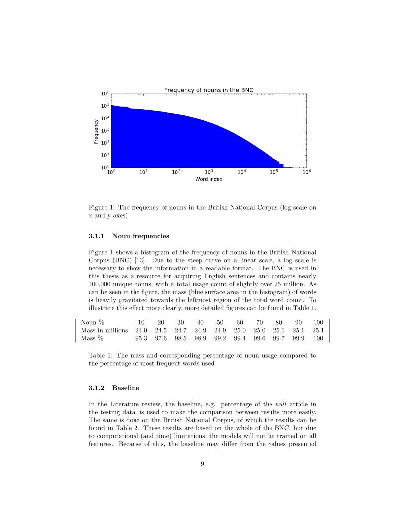
Figure 1: The frequency of nouns in the British National Corpus (log scale onx and y axes)

3.1.1 Noun frequencies

Figure 1 shows a histogram of the frequency of nouns in the British NationalCorpus (BNC) [13]. Due to the steep curve on a linear scale, a log scale isnecessary to show the information in a readable format. The BNC is used inthis thesis as a resource for acquiring English sentences and contains nearly400,000 unique nouns, with a total usage count of slightly over 25 million. Ascan be seen in the figure, the mass (blue surface area in the histogram) of wordsis heavily gravitated towards the leftmost region of the total word count. Toillustrate this effect more clearly, more detailed figures can be found in Table 1.

Noun % 10 20 30 40 50 60 70 80 90 100Mass in millions 24.0 24.5 24.7 24.9 24.9 25.0 25.0 25.1 25.1 25.1Mass % 95.3 97.6 98.5 98.9 99.2 99.4 99.6 99.7 99.9 100

Table 1: The mass and corresponding percentage of noun usage compared tothe percentage of most frequent words used

3.1.2 Baseline

In the Literature review, the baseline, e.g. percentage of the null article inthe testing data, is used to make the comparison between results more easily.The same is done on the British National Corpus, of which the results can befound in Table 2. These results are based on the whole of the BNC, but dueto computational (and time) limitations, the models will not be trained on allfeatures. Because of this, the baseline may differ from the values presented

9

here. The percentages are only based on sentences at least containing one NP,which resulted in 4,927,667 sentences containing a total of 10,841,032 NPs. Thisresults in an average of 2.2 NPs per sentence.

Article OccurenceNull 59.7%The 27.2%A/an 13.1%

Table 2: Occurrence of articles in the BNC

3.1.3 Cutoffs

Since, due to the ‘long tail’, not all nouns can be represented as a feature, ametric is used that quantifies how words are split based on their frequency in theBNC. The words are split in three ‘ordinarity groups’, marked by two cutoffs.These groups are ‘common’, ‘rare’ and ‘noise’, which are the result of the ‘rarecutoff’ and the ‘noise cutoff’. All common words will be represented by theone-hot vector and both the common and rare groups will be represented viathe cluster as described in more detail in Section 3.3.5. The noise group willnot be represented by either feature. Not representing these words is thoughtof to reduce training on words that are likely to not be of significant use andwill not occur in real-world situations. A visual representation of how the datais split using these cutoff values can be found in Table 5.

Frequency Ordinarity0... noise45... rare910... commonn

Table 3: An example of word category distribution with noise cutoff 5 and rarecutoff 10

10

3.1.4 Mass nouns

To be able to make a distinction between mass and count nouns, a methodhas been devised that determines which nouns are countable and which arenot. This information as feature is very descriptive, since mass nouns cannotbe used with all articles. For example, scissors, meat, and English do not haveboth a singular and a plural form and the indefinite article a/an cannot be usedwith any of these. The feature, although informative, is not a perfect heuristic.Some words, like water, are generally regarded as a mass noun (you cannot puttwo water(s) in a bucket), but are still able to be used with a (water can alsorepresent a glass of water).

To identify the mass nouns from the others, all nouns in the BNC are counted.To estimate which words share a common base, a stemmer is used. In this casethis is the Snowball stemmer as made available by the NLTK package [1]. Usingthe stem, all variations of the same word can be grouped together. Per steman evaluation is made: If a certain instance of a word occurs significantly moreoften than the other forms, the word itself can be regarded as (practically) amass noun. The thresholds for this value have been empirically estimated, byensuring some known mass nouns to be marked as such3. Words are saved asbeing mass if one form takes up either more than 90% of the base concept’sfrequency, but only if the total frequency (the sum of the frequencies of allwords with the same stem) is above 10. If this would not be done, many rarewords could be incorrectly flagged as being a mass noun.

3.2 Features

3.2.1 Reference

The features used for the reference model are based on the research done byDe Felice and Pulman [4] and Han, Chodorow, and Leacock [6], as previouslydiscussed. These are:

• Head noun vectorThe one-hot vector representing the head noun. To construct this vector,output as described in Section 3.3.4 is used. In this case, the list of nounsis consulted. This list is, based on the rare cutoff, set to only save the firstwords until the index value. Since the word list is placed in descendingorder of word frequency, the most occurring words are left. A vectorconsisting of zeros with this same size is constructed and the index atwhich the head noun occurs in the list, becomes a 1 in the vector. Thevalue at which the cut is done is varied for the head noun.

• Head noun noiseA flag feature based on the frequency of the head noun. If the word falls

3These words were scissors and rice.

11

in the noise category, the word is flagged as such.

• Head noun numberMarks if the head noun is singular or plural. This information is gatheredusing the POS tag of the word, which holds separate tags for these cases.The POS tags for singular nouns are NN and NNP. Plural nouns aredenoted with NNP and NNPS.

• Head noun typeGathered from the output described in Section 3.3.4, marks if the headnoun is a count or a mass noun.

• Head noun named entityMarks if the head noun is a concept, like a person or place. This infor-mation is also gathered using the POS tag of the word, namely the NNPand NNPS tags.

• Preposition modificationMarks if a preposition is used inside the noun phrase. This is done bychecking if one of the words in the noun phrase is tagged as such. Thecorresponding POS tag is IN.

• Preposition modification vectorThe one-hot representation of the found preposition. How this vectoris built is explained at the Head noun vector feature. A significant dif-ference between nouns and prepositions is the needed cardinality of thevector. Since there are orders in magnitude fewer different prepositionsthan nouns, all prepositions used in the BNC can be represented. The car-dinality of this vector (and thus total unique occurences of prepositions inthe BNC) is 1,701.

• Head noun object of prepMarks whether the head noun is the object of the found preposition. Thisis the case if the first noun after the preposition is the head noun.

• Adjective modificationMarks whether an adjective modifies the head noun. This is determinedby checking of an adjective occurs in the noun phrase, before the headnoun.

• Adjective modification vectorThe one-hot encoding representation of the found adjective. How thisvector is built is explained at the Head noun vector feature. Like nouns,there exist many adjectives (close to 140,000 in the BNC). Becasue of this,the cardinality of this vector is set to 4,000. This allows 90% of all wordusage to be represented, but due to the ‘long tail’, only 2.9% of all possiblewords are covered.

• Adjective gradeMarks which grade the found adjective is. Many adjectives have a com-

12

parative (good → better) and/or a superlative (good → best) form. Thegrade of the adjective can be read from the POS tag, which denote theadjective, comparative and superlative as JJ, JJR, and JJS respectively.

• Noun phrase relationMarks if a noun phrase is the object or subject of a verb. This is testedby checking the siblings of the noun phrase in the tree structure. If a verbcan be found in one of these, the np is marked as the object. Else, it ismarked as subject.

• POS ±3Marks the three POS tags around the article, if one exists. If the article isnull, the POS tags around the head noun are given instead. There are 36POS tags specified in the Penn Treebank POS tagset. To accomodate thepossibility of there not being three words on either side, a one-hot vectorof size 37 is used to represent a single tag.

3.2.2 Word categories

The word categories are represented by being part of a certain cluster. Howthese clusters are made can be found in Section 3.3.5. All clusters have anindex, which allows for the representation of the cluster as a one-hot vector,similar to how the nouns, prepositions and adjectives are represented.

3.2.3 Context

The implementation of context is kept simple: A single value is used for thisfeature, which is 1 if the head noun of the noun phrase occurs in the previousX sentences. If this is not the case, its value is 0.

3.3 Pre-processing

Figure 2: Overview of pre-processing

13

Figure 2 provides an overview of the steps in which the pre-processing is divided.In short, the British National Corpus [13] is tagged with Penn Treebank POStags and parsed using a CCG parser. The parsed trees, together with the resultof a procedure that analyses the frequency of certain POS tags, and clustersfrom the Google News mappings are combined to create feature vectors. Thesecan then be used as input for a machine learning algorithm. The followingsections will discuss the implementation of these steps in more detail.

3.3.1 Extracting from corpus

The resource used for the conversion of English language to the final form offeature vectors is the British National Corpus (BNC). This corpus is heavilyannotated, which is very useful for many applications. However not in this case.The words in the BNC are provided with POS tags, but are from the BNCBasic (C5) Tagset and not the Penn Treebank POS tag, which is required forthe parser that will be used at a later point. Therefore, only the sentences inthe BNC itself are useful and need to be extracted so the required informationcan be added in the subsequent steps.

The BNC consists of around 4000 files, placed in a three-level-hierarchy. Thefiles themselves are in an XML format that with tags for all sentences and wordswith multiple pieces of information. An example of how a sentence is representedcan be found in Figure 3. To extract the ‘raw’ sentences from this structure,the hierarchy is traversed and the files are read. The containing XML structureis read and the sentences, without any tags, are saved.

<s n="7">

<w c5="PNP" hw="i" pos="PRON">I </w>

<w c5="AV0" hw="particularly" pos="ADV">particularly </w>

<w c5="VVD" hw="wish" pos="VERB">wished </w>

<w c5="TO0" hw="to" pos="PREP">to </w>

<w c5="VVI" hw="clarify" pos="VERB">clarify </w>

<w c5="AVQ" hw="why" pos="ADV">why </w>

<w c5="PNI" hw="one" pos="PRON">one </w>

<w c5="VVZ" hw="study" pos="VERB">studies </w>

<w c5="NN1" hw="history" pos="SUBST">history </w>

<mw c5="AV0">

<w c5="PRP" hw="at" pos="PREP">at </w>

<w c5="DT0" hw="all" pos="ADJ">all</w>

</mw>

<c c5="PUN">.</c>

</s>

Figure 3: Fragment of BNC XML structure for the sentence “I particularlywished to clarify why one studies history at all.” (indented for readability)

14

3.3.2 Tagging

To provide the Penn Treebank POS tags to the extracted sentences, the StanfordLog-linear Part-Of-Speech Tagger [15] is used. The parser requires the taggedsentences to be in a slightly different format than what the Stanford taggeroutputs. To accomodate this, another script processes the stanford output to areadable output for the next step. Sentences are now structured as can be seenin Figure 4.

The|DT mean|JJ density|NN of|IN Mercury|NNP indicates|VBZ that|IN

its|PRP$ interior|NN is|VBZ substantially|RB different|JJ from|IN

the|DT interiors|NNS of|IN the|DT other|JJ terrestrial|JJ planets

|NNS

Figure 4: Example of the tagged sentence “The density of Mercury indicates thatits interior is substantially different from the interiors of the other terrestrialplanets.”

3.3.3 Parsing

To parse the tagged sentences into tree structures, a CCG parser called Easy-CCG developed by Lewis and Steedman [8] is used. One of the reasons forthis choice is because of the high speed (150 sentences per second), which isnecessary to prevent pre-processing taking up too much time. How this outputis formatted can be seen in Figure 5.

(<T S[dcl] 1 2>

(<L NP PRP PRP It NP>)

(<T S[dcl]\NP 0 2>

(<T (S[dcl]\NP)/(S[pss]\NP) 0 2>

(<L (S[dcl]\NP)/(S[pss]\NP) VBZ VBZ is (S[dcl]\NP)/(S[

pss]\NP)>)

(<L (S\NP)\(S\NP) RB RB not (S\NP)\(S\NP)>)

)

(<T S[pss]\NP 0 2>

(<L S[pss]\NP VBN VBN transmitted S[pss]\NP>)

(<L (S\NP)\(S\NP) IN IN from (S\NP)\(S\NP)>)

)

)

)

Figure 5: Example of the CCG parsed “It is not transmitted from.” (indentedfor readability)

15

The output of the EasyCCG parser produces a tree structure that is not directlyreadable into a data structure. Additionally, many POS tags created by theCCG parser are not needed for further usage, since many tags hold informationabout the sentence structures of their children nodes. This information is notnecessary for further processing, and to both reduce the size of the final file andmake it more human-readable for intermediate evaluation, it is removed in thisstep. An example of the final format for the tree structures can be found inFigure 6.

[’S’,

[’S’,

[’NNP’, ’Gim’],

[’NP’,

[’PRP’, ’me’],

[’NP’,

[’RP’, ’back’]

]

]

],

[’NP’,

[’NP’,

[’DT’, ’that’],

[’NN’, ’bottle’]

],

[’NP’,

[’IN’, ’of’],

[’NP’,

[’NP’,

[’NP’,

[’NNP’, ’Sainsbury’]

],

[’POS’, "’s"]

],

[’NNP’, ’Cider’]

]

]

]

]

Figure 6: Example of the final parsed sentence “Gimme back that bottle ofSainsbury’s Cider.” (indented for readability)

16

3.3.4 Frequency analysis

To represent nouns, adjectives and prepositions as vectors, a script is used thatloops through all trees and counts the words which are either a noun, adjectiveor preposition. The word lists are placed in descending order based on thegathered frequencies. Using this information, the X most occuring words inthese tags can be represented as a vector in feature creation. Additionally, asdescribed in Section 3.1.4, the mass nouns are identified and saved as well.

3.3.5 Clustering

A popular toolkit for the creation of word embedding mappings is word2vec,developed by Mikolov et al. [9]. They also provide pre-trained vectors trainedon a part of the Google News dataset (∼100 billion words). The model contains300-dimensional vectors representing 3 million words [10].

The Google News mappings are read using the gensim library [12], which allowsconvenient reading of the binary file in which the mappins are stored. The map-pings are then converted to another data format, so they can be fed as inputto a clustering algorithm. This is done by using the scikit-learn library’s Mini-BatchKMeans algorithm [11]. This algorithm performs very similar to k-means,except for the fact that it works with smaller batches to decrease computationtime.

The amount of clusters over which the word vectors are spread can be varied.There are no specific initial assumptions made on this value, but it is expectedthat more clusters will lead to more specific word categories, which might leadto more specific word groupings. It is expected that the specificity of the wordgroups may have a positive impact on the performance of the feature. Variationsare tested and can be found in the Results section (Section 4).

3.3.6 Feature creation

The final step in pre-processing is to collect the data from the parsing trees,word counts, mass nouns, and clusters to construct features from these sourcesthat can be used for machine learning.

A general idea of the construction of the features is outlined in Procedure 1.The pre-process is separated in three parts, extracting information from thenoun phrase, the sentence and the context. However, not all noun phrasesare useful for this process. The ones that contain determiners like ‘those’ or‘every’ are sure to not need an article and are therefore marked invalid. Thesecases are not converted to feature vectors since they can be recognised easily bypre-processing steps.

17

Procedure 1 Overview of feature constructionfor all sentenceTree← file do

for all nounPhraseTree← sentenceTree dovalidFeature := checkV alid(nounPhraseTree)if validFeature then

getNounPhraseFeatures()getSentenceFeatures()getContextFeatures()

end ifend for

end for

3.4 Machine learning

Due to the large amount of feature vectors and these vectors having a highcardinality, not all data be trained at once since this does not fit in memory.Scikit-learn [11] offers several machine learning algorithms that can be used out-of-core, meaning it does not require all data to be present in memory at once.Instead, it is able to train multiple ‘batches’ after each other. The algorithmsavailable with this function are:

• Naive Bayes for multinomial models

• Naive Bayes for Bernoulli models

• Perceptron

• Stochastic Gradient Descent

• Passive Agressive Algorithms

For all results that can be found in this thesis, the machine learning algorithmsare trained on 75% of the data and tested on the remaining 25%. Duringtraining, each batch is randomly split into a training and a testing set. Thetraining set is trained upon for a set amount of iterations. Afterwards, the testset is used to evaluate the classifier at that point. After every batch, especiallyat the early iterations, the performance of the classifier increases rapidly.

To evaluate the final version of the classifier, a separate evaluation script is used.Since every model is trained on a random sample of data, this evaluation cannotbe done on the same data for every model. Therefore, all intermediate test setsare saved inbetween the training sessions to be used for this purpose. Becauseof the randomness of train-test splitting and the variety of text sources in theBNC there are no concerns that the model is optimised for the testing data.

To determine which algorithm suits the data best, possible models need to betrained and compared. Apart from the choice of algorithm itself, some initial

18

values can be set to improve the performance as well. The process of finding themost suitable algorithm and its parameters is described in the following section.

4 Results

This section is split in four parts. First, a reference model is constructed. Then,the influence of different values for the rare cutoff is evaluated. Finally, usingthe reference model as a comparison measure, the impact of the word categoriesare evaluated, followed by the context feature.

4.1 Building a reference model

To start, a model needs to be made that works only on the reference features,which are discussed in Section 3.3.6. Since several machine learning algorithmsare available, the first step in establishing the reference model is to determinewhich algorithm suits the data best. Table 4 shows a comparison of the availablealgorithms trained on 75,000 items and tested on 25,000.

The head noun is vectorised with a rare cutoff of 10, which results in the headnoun vector feature to be of size 68,578. This value enables the feature torepresent 97.5% of noun usage, but still only 18.6% of possible nouns.

Algorithm AccuracyBaseline 55.0%Naive Bayes multinomial 67.0%Naive Bayes Bernoulli 65.5%Perceptron 61.1%Passive Agressive Algorithms 60.9%Stochastic Gradient Descent 65.8%

Table 4: Comparing the performance of different machine learning algorithmson the reference data

The Naive Bayes model for multinomial data achieves the highest accuracycompared to the other options. However, it does not achieve the scores ofpreviously discussed research. There is no definite reason to explain this, butit is clear that the model is predicting based on the features. The baseline inthe table again refers to the frequency of the most occurring class, null, and thedifference between Naive Bayes and the baseline is significant. Therefore, theNaive Bayes for multinomial data trained on only the reference features will beused for all comparisons when regarding the reference model.

19

4.2 Cutoff influence

To investigate the impact of the head noun representation for the common cat-egory, Table 5 shows an overview of different rare cutoff values, the appropriatemass of noun usage that can be represented and the accuracy achieved. Notethat no baseline is mentioned in this table, since the goal of this test is notto search for the best outcome, but rather to see what shifting the rare cutoffmeans for performance. The models are trained on 750,000 items and tested on250,000.

Rare cutoff Noun mass Accuracy10 97.5% 68.1%50 93.9% 67.9%

1,000 73.7% 67.1%5,000 47.3% 64.5%10,000 31.8% 63.2%

Table 5: Accuracy for different rare cutoff values

As can be seen in the table, the higher the rare cutoff is set (and thus whenthe represented noun mass decreases), the lower the accuracy of the classifierbecomes. A significant difference can be seen between cutoff 1,000 and 5,000,which decreased the noun mass by 26.4% and lowered the accuracy by a rel-atively large portion. The difference observed one row above, from cutoff 50to cutoff 1,000, is relatively small compared to the other decrease. A mass de-crease of 20.2% leads to just 0.8% decrease in accuracy. This is to be expected,though. As observed in the analysis on the data (Section 3.1), word usage is dis-tributed on a near-logarithmic scale. Impact on accuracy is therefore expectedto decrease the most when reaching noun masses closer to zero.

4.3 Word categories

To test the impact of the word clusters, the reference model is compared toa model which is trained both the reference features and the noun categoryfeature. The comparison is made using two rare cutoff features: 10 and 1,000.Even though the lowest possible cutoff value is normally preferred, the highercutoff is also regarded because it creates a larger portion of rare words, whichallows the word category feature to be trained and tested on more instances.

For both values of the rare cutoff, three models are compared: The referencemodel as described in previous sections, and two variations of models whichhave been trained on both the reference features and the word category feature.These differ in the cluster size, which determines the specificity of the categories(greater size, more specific clusters).

20

The performance of previous models have only been tested on all words inthe testing set. However, since the word categories are expected to show mostimpact on the rare words, which are not represented directly by a one-hot vector,and the percentage of words in this group is relatively low by definition, theaccuracy on all different word ordinarities (common, rare, noise) are evaluated.The results are displayed in Table 6. The models are all trained on 75,000 itemsand tested on 25,000.

Model Rare cutoff Common Rare Noise All wordsBaseline 10 54.0% 71.1% 76.3% 55.3%

1,000 51.2% 62.2% 75.7% 55.2%Reference 10 66.0% 68.6% 77.5% 66.6%

1,000 65.2% 63.5% 76.6% 65.4%Clusters 1,000 10 64.4% 65.1% 76.8% 65.3%

1,000 64.4% 65.2% 75.8% 65.2%Clusters 10,000 10 65.0% 70.2% 78.4% 65.8%

1,000 64.4% 66.8% 76.1% 65.6%

Table 6: Accuracy when clusters are used, evaluated on different word ordinar-ities

From these results a few observations can be made. To start, the baseline per-centage seems to increase when words become more rare. A possible explanationfor this is the fact that more rare words are more specific, which can be used inless different ways and are therefore less compatible with all articles. However,a more in depth study will be required to investigate the exact reason behindthis.

It also seems that that the reference model is using its predictive power on thecommon words, which may indicate that the other reference features beside theone-hot vector for the head noun are not utilised very well. This would alsoexplain the relatively low accuracy that the model achieves when compared tothe models which it is based on.

The results of the cluster model is somewhat positive. The accuracy for themodels when tested on all word ordinarities stay similar, but when regarding thecommon words only, the model using 1,000 clusters shows a significantly higheraccuracy than the reference and cluster model with a higher cluster count inthe same situation. This result shows promise, but is not sufficient to confirmwhether the feature works well in all cases.

4.4 Context

To evaluate the context feature, the baseline and reference models are comparedto two models that incorporate context. Results on this can be found in Ta-

21

ble 7. The number after “Context” regards the context size: The amount ofsentences that are evaluated to contain the head noun. The models are trainedon 750,000 items and tested on 250,000. A rare cutoff of 50 is used to speed upthe evaluation process.

Model AccuracyBaseline 55.4%Reference 67.9%Context size 1 68.3%Context size 5 68.4%

Table 7: Accuracy when context is introduced

The models trained on the additional context feature have achieved a slightlyhigher accuracy, but the significance of this is debatable. However, even thoughthe improvement is small, if implemented in a more complex way, the feature isexpected to affect the model in a positive way rather than negative.

5 Conclusion

The reference classifier performed with a lower accuracy than desired, but wasuseful for the evaluations nonetheless. The steep curve of word usage whencompared to its occurrence was as noticeable as expected regarding the deter-mination of the size of the one-hot vector to represent a noun.

The individual evaluation on different word ordinarities suggests a possible prop-erty of article usage that was not found in previous research: Highly frequentwords seem to be used with more different articles than infrequent words.

The word category feature seems to provide a small positive impact on repre-senting infrequent words by using a relatively small sized vector, but the singlesignificant value that was observed is not enough to make a final judgementon the utility of the feature. The implementation of the cluster feature in thisthesis has shown no significant impact.

6 Discussion

It was decided quite early in the project to base the reference model largely onthe paper by De Felice and Pulman [4], but due to their features being heavyon semantics, a large portion of the available time for the project was spent onthis instead of the exploration of new features. If faced with the same situationagain, I would have preferred to base it off the features used by Han, Chodorow,and Leacock [6], since most of their features were based on a more simple idea

22

of representing all POS tags in a given NP. Perhaps time spent on this goalinstead of the conducted plan would have allowed more time to be spent on thenew ideas, but at this point it is difficult to make such a prediction confidently.

In the last week of the project, it was discovered that named entities (includingnames) have been part of the noun set. This has also been done by De Felice etal., but would not have been necessary to do, since Named Entitity Recognitioncan also be used to solve that problem. The Named Entity feature implementedas part of the reference model was also quite a simplified approach, since itrelied on the Stanford Tagger to assign the proper noun tag to named entities.

7 Future research

From the results on word categories, it was observed that less frequent occurringwords had a higher baseline percentage for the null article. A possible reasonfor this phenomenon is discussed, but more analytic methods could be used tomap the frequencies of different articles to the word occurence. It may be thatsome relation can be found between these variables.

The context feature has been the least explored feature in the thesis with onlya very basic implementation being evaluated. Only the literal occurence of thehead noun is evaluated in this thesis, but a logical next step would be to alsoregard similar words that have occurred. Lemmatising or stemming could beused for this, but word embedding vectors could also be used to calculate thecosine similarity between the headnoun and previous (head) nouns.

The approach for creating word categories could be easily used for other lan-guages as well, for example on Dutch. Word embedding is language independent,which makes it possible to find categories in many natural languages.

8 Acknowledgements

I want to thank the supervisor of my thesis, Dr. Tejaswini Deoskar, for herguidance throughout the project and suggestions that pushed me in the rightdirection when it was needed. The experience of working on this project hasbeen very educational, which can be accredited to her.

23

References

[1] Steven Bird, Ewan Klein, and Edward Loper. Natural language processingwith Python. ” O’Reilly Media, Inc.”, 2009.

[2] Eugene Charniak. “Immediate-head parsing for language models”. In: Pro-ceedings of the 39th Annual Meeting on Association for ComputationalLinguistics. Association for Computational Linguistics. 2001, pp. 124–131.

[3] Rachele De Felice. “Automatic error detection in non-native English”.PhD thesis. University of Oxford, 2008.

[4] Rachele De Felice and Stephen G Pulman. “A classifier-based approach topreposition and determiner error correction in L2 English”. In: Proceed-ings of the 22nd International Conference on Computational Linguistics-Volume 1. Association for Computational Linguistics. 2008, pp. 169–176.

[5] Rachele De Felice and Stephen G Pulman. “Automatically acquiring mod-els of preposition use”. In: Proceedings of the Fourth ACL-SIGSEM Work-shop on Prepositions. Association for Computational Linguistics. 2007,pp. 45–50.

[6] Na-Rae Han, Martin Chodorow, and Claudia Leacock. “Detecting errorsin English article usage by non-native speakers”. In: (2006).

[7] John Lee, Joel Tetreault, and Martin Chodorow. “Human evaluation ofarticle and noun number usage: Influences of context and constructionvariability”. In: Proceedings of the Third Linguistic Annotation Workshop.Association for Computational Linguistics. 2009, pp. 60–63.

[8] Mike Lewis and Mark Steedman. “A* CCG Parsing with a Supertag-factored Model.” In: EMNLP. 2014, pp. 990–1000.

[9] Tomas Mikolov et al. “Efficient estimation of word representations in vec-tor space”. In: arXiv preprint arXiv:1301.3781 (2013).

[10] Tomas Mikolov et al. Google Code Archive: word2vec. July 30, 2013. url:https://code.google.com/archive/p/word2vec/.

[11] F. Pedregosa et al. “Scikit-learn: Machine Learning in Python”. In: Jour-nal of Machine Learning Research 12 (2011), pp. 2825–2830.

[12] Radim Rehurek and Petr Sojka. “Software Framework for Topic Modellingwith Large Corpora”. English. In: Proceedings of the LREC 2010 Work-shop on New Challenges for NLP Frameworks. http://is.muni.cz/publication/884893/en. Valletta, Malta: ELRA, May 2010, pp. 45–50.

[13] Oxford University Computing Services. The British National Corpus. url:http://www.natcorp.ox.ac.uk/.

[14] Joel R Tetreault, Claudia Leacock, and McGraw-Hill Education CTB.“Automated Grammatical Error Correction for Language Learners.” In:COLING (Tutorials). 2014, pp. 8–10.

[15] Kristina Toutanova et al. “Feature-rich part-of-speech tagging with acyclic dependency network”. In: Proceedings of the 2003 Conference ofthe North American Chapter of the Association for Computational Lin-guistics on Human Language Technology-Volume 1. Association for Com-putational Linguistics. 2003, pp. 173–180.

24

[16] Jenine Turner and Eugene Charniak. “Language modeling for determinerselection”. In: Human Language Technologies 2007: The Conference of theNorth American Chapter of the Association for Computational Linguis-tics; Companion Volume, Short Papers. Association for ComputationalLinguistics. 2007, pp. 177–180.

25