Improvement Theory and its Applications - Chalmersdave/papers/hoots97.pdf · Improvement Theory and its Applications ... weak head normal forms. ... isfying the rules given in Figure

Improvement Theory and itsApplications

David Sands Chalmers University and the University of Goteborg

Abstract

An improvement theory is a variant of the standard theories of observa-tional approximation (or equivalence) in which the basic observations madeof a functional program’s execution include some intensional information about,for example, the program’s computational cost. One program is an improve-ment of another if its execution is more efficient in any program context. Inthis article we give an overview of our work on the theory and applications ofimprovement. Applications include reasoning about time properties of func-tional programs, and proving the correctness of program transformation meth-ods. We also introduce a new application, in the form of some bisimulation-like proof techniques for equivalence, with something of the flavour of San-giorgi’s “bisimulation up-to expansion and context”.

1 Introduction

An improvement theory is a variant of the standard theories of observational ap-proximation (or equivalence) in which the basic observations made of a program’sexecution include some intensional information about, for example, the program’scomputational cost. One program is an improvement of another if its execution ismore efficient in any program context.

In this article we survey a number of applications of a particular improvementtheory developed for a small untyped functional language.

The initial motivation for considering such relations was to support a simple cal-culus for reasoning about time behaviour of non-strict functional programs (Sands1993). From this work it was a natural step to consider a more general class ofimprovement theories for functional languages, providing contextually robust the-ories of optimisation (Sands 1991).

However, the real pay-off for this study is not in reasoning about efficiency prop-erties per se, but in reasoning about equivalence: The Improvement Theorem (Sands1995b) provides a condition for the total correctness of transformations on recur-sive programs. Roughly speaking, the Improvement Theorem says that if the localsteps of a transformation are contained in a particular improvement theory, thencorrectness of the transformation follows. This result has furnished:�

To appear: Eds. A. Gordon and A Pitts, Higher-Order Operational Techniques in Semantics,Cambridge University Press, 1997.

1

2 Sands

� an equivalence-preserving variant of the classic Unfold-Fold transformationin a higher-order functional languages (Sands 1995b), and� the first correctness proofs for a number of well-known transformation meth-ods(Sands 1996a) (see also (Sands 1995a)).

New work reported in this article is the development of some proof techniques forequivalence based on the improvement theory, with something of the flavour ofSangiorgi’s “bisimulation up-to expansion and context”.

Overview

In the next section we introduce the syntax and semantics of the language used inthe remainder of the article. Section 3 introduces a simple improvement theory forthe language based on observing the number of recursive calls made during evalu-ation. We introduce proof techniques for establishing improvement, and introducethe tick algebra which facilitates the calculation of simple improvement properties.Section 4 considers the application which originally motivated the study of im-provement relations, namely the problem of time analysis of functional programs.Section 5 describes a correctness problem in program transformation. We presentThe Improvement Theorem, which shows, in principle, how the problem can besolved by using improvement. Section 6 illustrates this application by consider-ing a particular program transformation method. Finally, Section 7 introduces andillustrates some proof techniques for the equivalence of programs which can be de-rived from the Improvement Theorem.

2 Preliminaries

We summarise some of the notation used in specifying the language and its oper-ational semantics. The subject of this study will be an untyped higher-order non-strict functional language with lazy data-constructors.

We assume a flat collection of mutually recursive definitions of constants, eachof the form

�� , where �� is a closed expression. Symbols�, , � �� , range over

the constants, �� over variables and � , �� , �� over expressions. Thesyntax of expressions is as follows:� � � � � � �� (Variable; Recursive constant; Application)� �� (Lambda-abstraction)� �!�"$# �&% �')(�* ��+ �� '�(�*-, + � ,(Case expressions)

�/.102�13 (Constructor expressions and constants)�54�02��3 (Strict primitive functions)')(�* � .1062� 3 (Patterns)

Improvement Theory and its Applications 3

Somewhat improperly we will refer to the constants�, , etc., as function names,

or function calls. In general they need not be functions however.We assume that each constructor . and each primitive function 4 has a fixed ar-

ity, and that the constructors include constants (i.e. constructors of arity zero). Con-stants will be written as . rather than .10 3 . The primitives and constructors are notcurried – they cannot be written without their full complement of operands. Weassume that the primitive functions map constants to constants.

We can assume that the case expressions are defined for any subset of patterns7 '�(�* � �� ')(�* ,98 such that the constructors of the patterns are distinct. A variablecan occur at most once in a given pattern; the number of variables must match thearity of the constructor, and these variables are considered to be bound in the cor-responding branch of the case-expression.

A list of zero or more expressions �� , will often be denoted 2� . Application,as is usual, associates to the left, so 0$0;:�:�:�0 ��<6��3 �� 3;� , 3 may be written as �6<&�� , ,and further abbreviated to ��< 2� .

The expression written � 7 2�>= � 2��? 8 will denote simultaneous (capture-free) sub-stitution of a sequence of expressions 2��? for free occurrences of a sequence of vari-ables 2� , respectively, in the expression � . We will use @ , @ ? , A etc. to range oversubstitutions. The term FV 0 ��3 will denote the set of free variables of expression � ,and 2FV 0 ��3 will be used to denote a (canonical) list of the free variables of � . Some-times we will informally write “substitutions” of the form

7 2B= � 2� 8 to represent thereplacement of occurrences of function symbols 2 by expressions 2� . This is not aproper substitution since the function symbols are not variables. Care must be takenwith such substitutions since the notion of equivalence between expressions is notclosed under these kind of replacements.

A context, ranged over by C , C � , etc. is an expression with zero or more “holes”,D1E, in the place of some subexpressions; C D � E is the expression produced by replac-

ing the holes with expression � . Contrasting with substitution, occurrences of freevariables in � may become bound in C D � E ; if C D � E is closed then we say it is a closingcontext (for � ).

We write �GF � ? to mean that � and � ? are identical up to renaming of boundvariables. Contexts are identified up to renaming of those bound variables whichare not in scope at the positions of the holes.

2.1 Operational Semantics, Approximation and Equivalence

The operational semantics is used to define an evaluation relation H (a partial func-tion) between closed expressions and the “values” of computations. The set of val-ues, following the standard terminology (see e.g. (Peyton Jones 1987)), are calledweak head normal forms. The weak head normal forms, IJ�I � �I � ��&K WHNFare just the constructor-expressions .102��3 , and the Closures (lambda expressions),as given by I � .�0L2��3 �M�)��

4 Sands

The operational semantics is call-by-name, and H is defined in terms of a one-stepevaluation relation using the notion of a reduction context (Felleisen, Friedman, andKohlbecker 1987). If � HNI for some closed expression � then we say that � evaluatesto I . We say that � converges, and sometimes write � H if there exists a I such that� HNI . Otherwise we say that � diverges. We make no finer distinctions betweendivergent expressions, so that run-time errors and infinite loops are identified.

Reduction contexts, ranged over by O P , are contexts containing a single holewhich is used to identify the next expression to be evaluated (reduced).

Definition 1 A reduction context O P is given inductively by the following grammarO P � D�E �QO P � �R �!�";#>O P % � ')(�* � + �1� �� ')(�* , + � , �4S0;2.��6O PJ�12��3The reduction context for primitive functions forces left-to-right evaluation of thearguments. This is just a matter of convenience to make the one-step evaluationrelation deterministic.

Now we define the one step reduction relation. We assume that each primitivefunction 4 is given meaning by a partial function

D D 4 E E from vectors of constants (ac-cording to the arity of 4 ) to the constants (nullary constructors). We do not needto specify the exact set of primitive functions; it will suffice to note that they arestrict—all operands must evaluate to constants before the result of an application,if any, can be returned— and are only defined over constants, not over arbitraryweak head normal forms.

Definition 2 One-step reduction TU is the least relation on closed expressions sat-isfying the rules given in Figure 1.

O P D � E TU O P D � � E (fun)0 if � is defined by� �� V3O P D 0V�� 13)�6? E TU O P D � 7 �J= � �W? 8 E ( X )O P D �!�";#Y.Z-02��3N% � ��.Z-062�[Z 3 + � ZQ�� E TU O P D � Z 7 2��ZQ= � 2� 8 E (case)O P D 4�0;2. 3 E TU O P D . ? E (prim)0 if D D 4 E E 2. � . ? 3

Figure 1: One-step reduction rules

In each rule of the form O P D � E TU O P D �6? E in Figure 1, the expression � is referred toas a redex. The one step evaluation relation is deterministic; this relies on the factthat if �1� TU �� then �� can be uniquely factored into a reduction context O P and aredex �W? such that �1� � O P D �W? E . Let TU]\ denote the transitive reflexive closure of TU .


Definition 3 Closed expression � converges to weak head normal form I , � HNI , ifand only if � TU]\ I .

Using this notion of convergence we now define the standard notions of operationalapproximation and equivalence. We use is the standard Morris-style contextual or-dering, or observational approximation see e.g. (Plotkin 1975).The notion of “ob-servation” we take is just the fact of convergence, as in the lazy lambda calculus(Abramsky 1990). Operational equivalence equates two expressions if and only ifin all closing contexts they give rise to the same observation – i.e. either they bothconverge, or they both diverge.

Definition 4 1. � operationally approximates �^? , �G_` �W? , if for all contexts Csuch that C D � E , C D �6? E are closed, if C D � E H then C D ��? E H .

2. � is operationally equivalent to ��? , � `� �W? , if �>_` �W? and �6?�_` � .Choosing to observe, say, only computations which produce constants would giverise to slightly weaker versions of operational approximation and equivalence - butthe above versions would still be sound for reasoning about the weaker variants ofthe relation.

3 A Theory of Improvement

In this section we introduce a theory of improvement, as a refinement of the the-ory of operational approximation. Roughly speaking, improvement is a refinementof operational approximation which expression � is improved by ��? if, in all clos-ing contexts, computation using �^? is no less efficient than when using � , measuredin terms of the number of function calls (

�, , etc.) made. From the point of view

of applications of the theory to program transformation and analysis, the impor-tant property of improvement is that it is a contextual congruence—an expressioncan be improved by improving a sub-expression. For reasoning about improvementa more tractable formulation of the improvement relation is introduced and someproof techniques related to this formulation are used.

Variations on the Definition of Improvement There are a number of variationsthat we can make in the definition of improvement. We could, for example, ad-ditionally count the number of primitive functions called. Such variations mightbe used to give additional information about transformations. However, the factthat we count the number of recursive function calls in the definition of improve-ment will be essential to the Improvement Theorem presented in the next section;the Theorem does not hold if we use an improvement metric which does not countthese function calls.

We begin by defining a variation of the evaluation relation which includes thenumber of applications of the (fun) rule.

6 Sands

Definition 5 Define ��aTU �W? if � TU �W? by application of the (fun)rule; define �cbTU �W?if � TU �W? by application of any other rule.

Define the family of binary relations on expressions7 TU , 8 ,1d < inductively as fol-

lows: � TU <&� ? if �cbTU \ � ?� TUfe;g �h�W? if � bTUf\ �� aTU �� TUfe �W? for some �1� , �� .We say that a closed expression � converges in i (fun)-steps to weak head nor-

mal form I , written � H , I if � TU , I .

The determinacy of the one-step evaluation relation guarantees that if � H , I and� H ,�j I ? then I F I ? and moreover i � i ? . It will be convenient to adopt thefollowing abbreviations:� � H , def�lk IJ� � H , I � � H ,�mQn def� � H ,Jo iqpMr � � H mQn def��k is� � H ,�mQnNow improvement is defined in a way analogous to observational approximation:

Definition 6 (Improvement) � is improved by ��? , �ut` �W? , if for all contexts C suchthat C D � E , C D �6? E are closed, if C D � E H , then C D �W? E H mQ, �It can be seen from the definition that t` is a precongruence (transitive, reflexive,closed under contexts, i.e. �vt` �W? + C D � E t` C D �W? E ) and is a refinement of opera-tional approximation, i.e. �Jt` �W? + � _` �W? �

We also define a strong version of improvement which contains (by definition)operational equivalence:

Definition 7 (Strong Improvement, Cost-Equivalence) The strong improvementrelation t`Jw is defined by: � t`xw �W? if and only if � t` �W? and � ` � �W? .

The cost equivalence relation, y t` , is defined by: � y t` �W? if and only if � t` �W?and �W?�t` � .If P is a relation, then let PJz � denote the inverse of the relation, so that {|P~}~� +}�P>z � { . It is not difficult to see that tùw � 0 t` 3�� 0V�` 3 . This fact, and other relation-ships between the various preorders and equivalence relations we have consideredso far, are summarised in the Hasse diagram of Figure 2. In this lattice, the binarymeet (greatest lower bound) corresponds to the set-intersection of the relations, andthe top element, � , relates any two expressions.

3.1 Proving Improvement

Finding a more tractable characterisation of improvement (than that provided byDef. 6) is desirable in order to establish improvement laws (and the ImprovementTheorem itself). The characterisation we use says that two expressions are in the


�� _` _` z �� t` `� t` z �� t`Jw t` z �w� �y t` �FFigure 2: A � -semi-sub-lattice of preorders

improvement relation if and only if they are contained in a certain kind of simula-tion relation. This is a form of context lemma eg. (Milner 1977; Abramsky 1990;Howe 1989), and the proof of the characterisation uses previous technical resultsconcerning a more general class of improvement relations (Sands 1991). In (Sands1991), we abstracted over the way improvement is defined in terms of the oper-ational semantics, and following Howe (1989), we gave some conditions whichguarantee that the simulation relations are sound for reasoning about improvement.

Definition 8 A relation �R� on closed expressions is an improvement simulationif for all � , � ? , whenever � �R� � ? , if � H , I � then � ? H mQ, I � for some I � such thateither:

1. I � F .�0 �� , 3 , I ��F .10 �6? � �� W?, 3 , and � Z�� W?Z , 0-� KG��i 3 , or

2. I � �I � K Closures, and for all closed ��< , 0�I ��W<63 �� 0�I ��6<W3For a given relation �R� and weak head normal forms I � and I � we will abbre-

viate the property “(1) or (2)” in the above by I � ��l��I � .So, intuitively, if an improvement simulation relates � to �1? , then if � converges, ��?does so at least as efficiently, and yields a “similar” result, whose “components”are related by that improvement simulation.

The key to reasoning about the improvement relation is the fact that t` , restrictedto closed expressions, is itself an improvement simulation, and is in fact the largestimprovement simulation. Furthermore, improvement on open expressions can becharacterised in terms of improvement on all closed instances. This is summarisedin the following.

8 Sands

Let t� denote the largest improvement simulation. It is easy to verify that thisexists, and is given by the union of all simulation relations. Let t� b denote its ex-tension to open terms specified by � t� b �W? if and only if � @ t� �W? @ for all closingsubstitutions @ .

Lemma 1 (Improvement Context-Lemma) For all � , ��? , ��t` �W? if and only if� t� b �W? .The most important part of the lemma, that t� b&� t` , can be proved by a straightfor-ward application of Howe’s method (Howe 1989), as illustrated in (Sands 1991).We omit the proof here. The proof of the “completeness” part of the lemma, that� t` � ? implies � t� b � ? , is rather more involved than the proof of the correspondingproperty for operational approximation. We give an outline of the main ingredients:� Characterise t� inductively in the form � Z�� t� Z (where t� Z is “simulation up

to a depth � ”). Then ��t� �W? implies that there exists a smallest r �c� suchthat ��t� n �W? .� It is sufficient to assume � and � ? closed, and to show that �l�t� � ? implies��t` � ? . By induction on the minimal r above, this can be done by building acontext which distinguishes � and � ? . This in turn depends on the existence ofcontexts which can magnify any non-zero computational cost by an arbitrarydegree.

The lemma provides a basic proof technique:

to show that �|t` �W? it is sufficient to find an improvement-simulationcontaining each closed instance of the pair.

An alternative presentation of the definition of improvement simulation is in termsof the maximal fixed point of a certain monotonic function on relations. In that casethe above proof technique is called co-induction. This proof technique is crucial tothe proof of the Improvement Theorem which follows in the next section. It canalso be useful in proving that specific transformation rules are improvements. Hereis an illustrative example; it also turns out to be a useful transformation rule:

Proposition 9 If the free variables of O P are distinct from the variables in ')(�* � ��W� ')(�*-, ,then O P D �!�";#Y� % � ')(�* � + � � :�:�: ')(�* , + � , Ey t` �!�"$#Y� % � ')(�* � + O P D � � E :�:�: ')(�* , + O P D � , EPROOF. We illustrate just the t` -half. The other half is similar. Let P be the rela-tion containing F , together with all pairs of closed expressions of the form:0�O P D �!�";# �W< % � . � 062� �3 + �� $. , 062� , 3 + � , E � �!�";# �W< % � . � 062� �3 =9O P D �� E ��. , 062� , 3 =�O P D � , E 3 (3.1)


It is sufficient to show that P is an improvement simulation. Suppose � P �1? , andsuppose further that � H , I . We need to show that ��? H mQ, I ? for some I ? such thatI�P � I ? . If ��F��6? then this follows easily. Otherwise � and ��? have the form of(3.1). Now since O P D �!�";# D1E % � . � 062� �$3 + �� $. , 062� , 3 + � , E is a reduction context,then we must haveO P D �!�"$# �6< % � . � 0W2� �3 + �1� ��;. , 062� , 3 + � , ETU e O P D �!^"$#Y.LZ�0L2�W?�? 3s% � . � 062� �;3 + �� . , 062� , 3 + � , Efor some expression .LZ-02�6?�?¡3 , and some ¢qpci and since each of these reductions is“in” �6< , we have matching reduction steps �!�";# �W<h% � . � 062� �;3 =9O P D �� E ��;. , 062� , 3 =[O P D � , ETU e �!�"$#Y.LZV02�6?�?¡3N% � . � 0W2� �3 =�O P D �1� E ��£. , 062� , 3 =9O P D � , ENow the former derivative reduces in one more step to O P D � Z 7 2��ZQ= � 2�W?�? 8 E , whilst thelatter reduces to O P D � Z E¤7 2��ZQ= � 2�W?�? 8 � Since reduction contexts do not bind variables,and since by assumption the free variables of the patterns are disjoint from the freevariables of O P , then these are syntactically equivalent, and so we conclude that �!�";# �W< % � . � 062� �;3 + O P D �� E ��. , 0W2� , 3 + O P D � , E H , IJ�The remaining conditions for improvement simulation (recall Def. 8 and the : � op-erator) are trivially satisfied, since I F � I , which implies I¥P � I as required. ¦3.2 The Tick Algebra

A particularly useful method for reasoning about improvement is to make use ofcertain identity functions, i.e., functions � such that for all � , � � `� � . Sometimes itis useful to consider functions which are the identity for expressions � of a certaintype (e.g., lists). The point of such functions is that they take time to do nothing; inother words � �§tùw � . Such functions facilitate the simple calculation of improve-ments, and are used extensively in applications of the theory. Here we consider thesimplest form of identity function, which we call the tick function.¨ �uFM©ª �« �where ©ª �« is an identity function, given by the definition©ª �« �� )��¡�The tick function will be our canonical syntactic representation of a single com-putation step. From the point of view of observational equivalence we can safelyregard it as an annotation, since

¨ � ` � � ; but from the point of view of improve-ment it is more significant. In particular, since the tick is a function call, from theoperational semantics it should be clear that� H , �¬� + ¨ � H , g � �

10 Sands

In terms of improvement, observe that¨ �Mt` � but �c�t` ¨ � (except if all closed

instances of � diverge).A key property regarding the tick function is that if function

�is defined by

� �� ,then � y t` ¨ �

In Figure 3 gives some simple laws for¨, the tick algebra, which we state with-

out proof. In the laws, O P ranges over reduction contexts, possibly containing freevariables. There is a related rule for propagation of ticks over contexts. If we de-fine an open context C to be strict if for all closing substitutions A , C D®YE A°¯±� where

is any closed expression such that ¯ . Then we claim that for all expressions� , C D ¨ � E t`Jw ¨ C D � E � The improvement is not reversible since the expression in the

hole may get duplicated.We will see see more of the tick functions when we come to consider applica-

tions of the theory.

� aTU � ?� y t` ¨ � ? � bTU \ � ?� y t` � ?¨ � t` � ¨ ��ht` ¨ ��ht` �� (similarly for ²³ w and ´�²³ )

O P D ¨ � E y t` ¨ O P D � E ¨ 4�0 � � �� , 3 y t` 4�0 � � �� ¨ � Z �� , 3¨ �!�";# �&% �. � 0�µ� �$3 + �� . , 0�µ� , 3 + � ,y t` �!�";# �h% �. � 01µ� �3 + ¨ �� £. , 0�µ� , 3 + ¨ � ,Figure 3: Tick laws

4 Time Analysis using Cost Equivalence

In this section we consider the application of the theory of improvement — and inparticular the theory of cost equivalence — to the problem of reasoning about therunning-time properties of programs. This section summarises some of the workdeveloped in Sands (1993).

Prominent in the study of algorithms in general, and central to formal activitiessuch as program transformation and parallelisation, are questions of efficiency, i.e.,the running-time and space requirements of programs. These are intensional prop-erties of a program—properties of how the program computes, rather that what itcomputes. In this section we illustrate how improvement can be used as a tool forreasoning about the running time of lazy functional programs.


In Sands (1990) we introduced a simple set of “naıve” time rules, derived di-rectly from the operational semantics. These concern equations on ¶ ��· , the “time”to evaluate expression � to (weak) head normal form, and ¶ ��·$¸ , the time to evaluate� to normal form. One of the principal limitations of the direct operational approachto reasoning is the fact that the usual meanings of “equality” for programs do notprovide equational reasoning in the context of the time rules. This problem moti-vated the development of a nonstandard theory of operational equivalence in whichthe number of computation steps are viewed as an “observable” component of theevaluation process. The resulting theory is the cost equivalence relation defined inthe previous section.

4.1 Motivation

As a motivating example for developing techniques to support reasoning about run-ning time, consider the following defining equations for insertion sort (written in aHaskell-like syntax)

isort [ ] = [ ]isort (h:t) = insert h (isort t)

insert x [ ] = [x]insert x (h:t) = x:(h:t) if ¹�pc�

= h:(insert x t) otherwise

As expected, ª " %�º�© requires »�0�i � 3 time to sort a list of length i . However, underlazy evaluation, ª " %�º�© enjoys a rather nice modularity property with respect to time:if we specify a program which computes the minimum of a list of numbers, by tak-ing the head of the sorted list

�,¼ ª¡½�ª ¼¿¾Q¼ � ��#�!�À§Á ª " %9ºÂ©

then the time to compute ¼ ªÃ½�ª ¼Ä¾Q¼ is only »�0�i 3 . This rather pleasing property ofinsertion-sort is a well-used example in the context of reasoning about running timeof lazy evaluation.

By contrast, the following time property of lazy “quicksort” is seldom reported.A typical definition of a functional quicksort over lists might be:

qsort [ ] = [ ]qsort (h:t) = qsort (below h t) ÅÅ (h:qsort (above h t))

where Æ�#RÇ %�È and !�Æ %RÉ # return lists of elements from © which are no bigger, andstrictly smaller than � , respectively, and ÅÅ is infix list-append. Functional accountsÊ

The example is originallydue to D. Turner; it appears as an exercise in informal reasoning aboutlazy evaluation in (Bird and Wadler 1988)[Ch. 6], and in the majority(!) of papers on time analysisof non-strict evaluation.

12 Sands

of quicksort are also quadratic time algorithms, but conventional wisdom would la-bel quicksort as a better algorithm than insertion sort because of its better average-case behaviour. A rather less pleasing property of lazy evaluation is that by replac-ing “better” sorting algorithm Ë�" %�º�© for ª " %�º�© in the definition of ¼ ª¡½�ª ¼¿¾Q¼ , we obtainan asymptotically worse algorithm, namely one which is Ì>0-i � 3 in the length of theinput. We will return to these examples.

4.2 Reasoning with Time

We outline how cost-equivalence can be used to help reason about the running timeof some simple lazy programs.

Time Equations The basic questions we wish to ask are of the form “How manyfunction-calls are required to compute the weak head normal form of expression e”.Typically � will not be a simple closed expression, but will contain a meta-variableranging over some first-order input values (normal forms). As is usual, the kindof answer we would like is a (closed form) function of the size of the input value,representing the exact, or asymptotic, cost. We will not be particularly formal aboutthe treatment of meta-variables, so most of our reasoning is as if we are dealing with(families of) closed expressions.

The basic idea is that we will use the instrumented evaluation � H , I as our cost-model. In order to abstract away from the result of a computation it is convenient tointroduce phrases of the form ¶ ��· : the time to compute expression � to weak headnormal form. In Sands (1993) we used rules along the lines of the following:

¶-I · � � ¶ ��· �ÎÍ ¶ � ? · if ��bTU � ?��Ï~¶ �W?®· if � aTU �W?This has an obvious shortcoming that it does not model the usual implementationmechanism. namely call-by-need, but proves to be adequate for many purposes.An approach to call-by-need is investigated in Sands (1993) also, but we will notconsider it here. Here we will mainly work with the cost-equivalence relation, andonly employ the time equations when it is notationally convenient to abstract awayfrom the result computed by the “top-level” expression.

Notation For iqÐM� , let, ¨ � denote the application of i ticks to expression � .

The following property follows easily from the tick algebra:

Proposition 10 For all closed expressions � ,1. � H , I implies � y t` , ¨ I2. � y t` , ¨ I ? K WHNF implies � H , I for some I such that I y t` I ? .


ª " %9ºÂ© �� )�°ÑQ� �!�"$#Y�°Ñ % �i��Ò + ½�ª Ç�Ó=�Ô + ª¡½ "$# º�© �Õ0 ª " %�º�© Ô 3ª¡½ "$# º�© �� )�Ö� �)�9ÑQ�� !^"$#>��Ñ % �½�ª Ç + �v= ½�ª Ç�Ó=QÔ + ª � ��pM� © ��# ½ �v=�0-�v=QÔ 3#�Ç ";#u�Ó=�0 ª¡½ "$# º�© �|Ô 3Figure 4: Insertion Sort

In terms of the time equations, we note that if � y t` , ¨ � ? then ¶ ��· � i×ÏØ¶ � ? · .The point of the proposition is that we can use y t` as a basis for reasoning aboutevaluation steps. Moreover, because y t` is a congruence, we can use it to simplifysubexpressions.

Insertion Sort Returning to the example given earlier, Figure 4 presents the in-sertion sort function, this time in the syntax of the language introduced earlier, butretaining the infix “:” list constructor.

The time to compute the head-normal form of insertion sort is relatively simpleto determine. We consider computing the head normal form of insertion sort ap-plied to some arbitrary (evaluated) list of integers Ù , =��=SÙ � = ½�ª Ç where iÚÐØ� .Let Û < denote the list ½�ª Ç and, for each �ÝÜMi , let Û�Z g � denote the list ÙRZ g � =�Û�Z . Thefollowing shows that the time needed to compute the first element of insertion sortis always linear in the length of the argument.

Proposition 11 For all � �M� there exist expression � ? and some value ÙÞK 7 Ù � ��Ù Z 8such that ª " %9ºÂ© Û�ZNy t` ß � Zàg ��á ¨ Ù|= � ?PROOF. By induction on � , and calculating using the tick algebra. In the base case0-� � � 3 we have ª " %9ºÂ© Û � y t` ¨ ªÃ½ ";# º�© Ù � 0 ª " %9ºÂ© Û <�3 y t` â ¨ Ù � = ½�ª Ç �

In the induction case 0-� � ¢�ÏM� 3 we calculate:ª " %�º�© Û e;g � y t` ¨ ªÃ½ ";# º�© Ù e;g � 0 ª " %�º�© Û e 3y t` ¨ ªÃ½ ";# º�© Ù e;g � ß � e;g �-á ¨ 0-Ù�= � ? 3 (Hypothesis)for some �6? and some Ù ? K 7 Ù � ��$Ù�e 8y t` � ¨ �!^"$# ß � e$g ��á ¨ 0�Ù�= �W?®3�% � ��y t` ß � ß e;g ��á g �-á ¨ ª � ÙRe;g � pMÙ © ��# ½ Ù�e;g � =QÙÞ= � ?#�Ç ";#YÙ|=�0 ª¡½ "$# º�© Ù�e$g ��W?®3y t` Í ß � ß e;g ��á g �-á ¨ Ù�e$g � =9ÙÞ= �W? if Ù�e;g � pMÙß � ß e;g ��á g �-á ¨ Ù|=�0 ª¡½ "$# º�© Ù�e$g ��6? 3 otherwise

14 Sands

Ë�" �� )��ÑQ� �!�";#Y��Ñ % �½�ª Ç + ½�ª Ç�Ó=�Ô + Ë�"�0ãÆR#�Ç %1È �|Ô 3 ÅÅ>0-�Ó=QË�"�0-!�Æ %�É #±�|Ô 3;3ÆR#�Ç %1È �� )��®�)��ÑQ�� !�";#u��Ñ % �½�ª Ç + ½�ª Ç�v=QÔ + ª � �Óp�� © ��# ½ �Ó=9ÆR#�Ç %�È ��Ô#�Ç ";#>ÆR#�Ç %�È ��Ô��Ñ�ÅÅ&��Ñ �� !�";#Y��Ñ % �½�ª Ç + �9Ñ�Ó=QÔ + �Ó=)0¤Ô$ÅÅ&�9Ñ 3Figure 5: Functional Quicksort

¦As a direct corollary we have ¶ ª " %�º�© Û)Z · ��ä ��ÏM� .Quicksort Now we consider a more involved example. The equations in Figure 5define a simple functional version of quicksort ( Ë�" ) using auxiliary functions Æ�#RÇ %�Èand !�Æ %�É # , and append written here as an infix function ÅÅ . Primitive functions forinteger comparison have also been written infix to aid readability. The definitionfor !�Æ %RÉ # has been omitted, but is like that of ÆR#�Ç %1È with the comparison “ � ” inplace of “ p ”.

The aim will be fairly modest: to show that quicksort exhibits its worst-case»�0�i � 3 behaviour even when we only require the first element of the list to be com-puted, in contrast to the earlier insertion sort example which always takes lineartime to compute the first element of the result. First consider the general case:

¶VË�" ��· � ��Ïå¢�Ïçæèèé èèê� if � y t` e ¨ ½�ª Çë Ë�"W0ãÆR#�Ç %1È �&Ô 3ÅÅ>0-��=�Ë�"�0-!�Æ %�É #±�&Ô 3$3Þì if � y t` e ¨ 0-�Ó=RÔ 3

From the time rules and the definition of append, this simplifies to

¶�Ë�" ��· � �íÏÚ¢¿Ï æé ê� if � y t` e ¨ ½�ª Ç�íÏ~¶VË�"60VÆ�#RÇ %�È �í� 3$· if � y t` e ¨ 0��Õ=QÔ 3 (4.1)

Proceeding to the particular problem, it is not too surprising that we will use non-increasing lists Ù to show that ¶�Ë�"�Ù · � Ì>0�i � 3 . Towards this goal, fix an arbitraryfamily of integer values

7 Ù�Z 8 ZÂî < such that ÙRZNpMÙ�ï whenever ��pÚð . Now define the


set of non-increasing lists7Rñ Z 8 Z d < by induction on � : let

ñ < denote the list ½�ª Ç , and,for each ¢Õ�M� let

ñ e$g � denote the list Ù�e;g � = ñ e .The goal is now to show that ¶-Ë�"�0 ñ , 3;· is quadratic in i . It is easy to see, instan-

tiating (4.1) that ¶�Ë�"�0 ñ e;g �3$· ��ä ÏM¶�Ë�"�0ãÆR#�Ç %�È ÙRe;g � ñ e 3;·but continuing with this simple style of reasoning we quickly see the limitationsof the “naive” operational approach to reasoning. Unlike the insertion-sort exam-ple where basic operational reasoning is sufficient (see (Sands 1993), where costequivalence is not used for the ª " %�º�© example), the successive calls to Ë�" becomeincreasingly complex. The key to showing that ¶�Ë�" ñ , · is quadratic in i is the iden-tification of a cost equivalence which allows us to simplify (a generalised versionof) the call to Æ�#RÇ %�È . To do this we will need another form of identity function.

Identity Functions on Lists We introduce another identity function, this time onthe domain of list-valued expressions. Let ò be the identity function on lists givenby ò �� )�� !�";#Y� % �½�ª Ç + ½�ª Ç�Ó=QÔ + 0��Ó=Qò�Ô 3As with the tick function, let ò , denote the i -fold composition of ò , where ò < � isjust � . It follows from this definition thatò , ½�ª Ç y t` , ¨ ½�ª Çò , 0��Ó=�Ô 3 y t` , ¨ 0-�Ó=�ò , Ô 3So ò , is an identity function for lists which increases the cost of producing eachconstructor in the list’s structure by i ticks. We use ò to characterise a key propertyof a certain call to ÆR#�Ç %�È :

Proposition 12 For all {�ÐM� , and �;�-ð such that ��pGðóp¥� ,ÆR#�Ç %1È 0�Ù1Zô�ò õ ñ ï 3 y t` ò õ g � ñ ï��PROOF. By induction on ð , using the tick algebra (it can also be proved straight-forwardly by coinduction).

16 Sands

Base: (ð � � ) Æ�#�Ç %�È 0-Ù1Zô�ò õ ñ <63 y t` ¨ �!�";#öò õ ñ <N% � �� 3y t` ¨ 0- �!^"$# , ¨ ½�ª Ç % � �� 3;3y t` õ g � ¨ 0 ½�ª Ç 3y t` ò õ g � ñ <Induction: (ð � ¢°ÏÄ� ) ÆR#�Ç %1È 0-Ù1Z-�ò õ ñ e;g �3y t` ¨ 0- �!^"$#&ò õ ñ e;g �N% � �� 3y t` õ g � ¨ 0� �!�";#öÙ�e;g � =Qò õ ñ e % � �� 3y t` õ g � ¨ 0 ª � Ù e;g � p�Ù Z © ��# ½ Ù e$g � =9ÆR#�Ç %�È 0-Ù Z �ò õ ñ e 3#�Ç ";#>ÆR#�Ç %1È 0-Ù Z �ò õ ñ e 3$3y t` õ g � ¨ 0�Ù�e$g � =9ÆR#�Ç %�È 0-Ù1Zô�ò õ ñ e 3;3y t` õ g � ¨ 0�Ù e$g � =Qò õ g � ñ e 3 (Hypothesis)y t` ò õ g � ñ e;g � ¦Now we can make use of the proposition in the analysis of quicksort. We considerthe more general case of ¶-Ë�"�ò õ ñ ï · . Considering the cases when ð � � and ð �¢¿ÏM� , and instantiating the general time equation gives:¶-Ë�"�0-ò õ ñ <63;· � �&ÏÚ{¶-Ë�"�0�ò õ ñ e$g �3;· � ä ÏÚ{>ÏM¶VË�"�0ãÆR#�Ç %1È Ù�e;g � ò õ ñ e 3;·� ä ÏÚ{>ÏM¶VË�"�0-ò õ g � ñ e 3$·Thus we have derived a recurrence equation which is easily solved; a simple induc-tion is sufficient to check that

¶-Ë�"[ò õ ñ , · � is0�i|ÏÚ÷ 3ä Ïå{°0�i|ÏM� 3 Ï~��Finally, since the

ñ , are just ò < ñ , , we have that the time to compute the weak headnormal form of Ë�" ñ , is quadratic in i :

¶VË�" ñ , · � iN0-i|ÏÚ÷ 3ä ÏM�R�Further Work Under a call-by-need computation model some computations areshared, so we would expect that, for example, 0ã�)��¡�×Ïø� 3 ¨ �ùy t` ¨ � where Ïis a primitive function. Instead, we get 0ã�)��¡�ÓÏl� 3 ¨ � y t` � ¨ � which can makecost equivalence unreliable for reasoning about non-linear functions. As we men-tioned earlier, the problems of reasoning about call-by-need are addressed in Sands(1993)— but not via a call-by-need theory of cost equivalence. Defining call-by-need improvement is not problematic. The problem is to find an appropriate contextlemma, and this is a topic we plan to address in future work. The applications ofthe Improvement Theorem introduced in the next section depend less critically on


the intentional qualities of improvement theorem. For these applications the call-by-name origin of our improvement theory is often advantageous, since for exam-ple unrestricted beta-reduction is an improvement for call-by-name. We do not yetknow whether the development of the next section will go through for a call-by-need theory.

5 The Improvement Theorem

In this section we motivate and introduce the ImprovementTheorem. The Improve-ment Theorem employs the improvement relation to prove the correctness of pro-gram transformations. The interesting point of this application is that the goal isnot to prove that program transformations improve programs per se, but simply toprove that they produce operationally equivalent programs.

5.1 The Correctness Problem

The goal of program transformation is to improve efficiency while preserving mean-ing. Source-to-source transformation methods such as unfold-fold transformation,partial evaluation (specialisation) and deforestation (Burstall and Darlington 1977;Jones, Gomard, and Sestoft 1993; Wadler 1990), are some well-known examples.These kind of transformations are characterised by the fact that� they utilise a small number of relatively simple transformation steps, and� in order to compound the effect of these relatively simple local optimisations,

the transformations have the ability to introduce new recursive calls.

Transformations such as deforestation (Wadler 1990) (a functional form of loop-fusion) and program specialisation (and analogous transformations on logic pro-grams) are able to introduce new recursive structures via a process of selectivelymemoising previously encountered expressions, and introducing recursion accord-ing to a “deja vu” principle (Jones, Gomard, and Sestoft 1993). In the classic unfold-fold transformation, it is the fold step which introduces recursion. See Pettorossiand Proietti (1995) for an overview of transformation strategies which fit this style.

The problem is that for many transformation methods which deal with recursiveprograms (including those methods mentioned above), correctness cannot be ar-gued by simply showing that the basic transformation steps are meaning preserving.

�Yet this problem (exemplified below) runs contrary to many informal—and some“formal”—arguments which are used in attempts to justify correctness of particulartransformation methods. This is the problem for which the Improvement Theoremwas designed to address.ú

One might say that there are two problems with correctness – the other problem is that it hasnot been widely recognised as a problem!

18 Sands

To take a simple example to illustrate the problem, consider the following “trans-formation by equivalence-preserving steps”. Start with the function º #�ûR#�! © whichproduces the “infinite” list of its argument:º #�ûR#�! © � �� Ó=)0 º #�ûR#�! © � 3Suppose the function © ! ª Ç computes the tail of a list. The following property canbe easily deduced: º #�ûR#�! © � ` � © ! ª Çà0 º #�ûR#�! © � 3 . Now suppose that we use this “localequivalence” to transform the body of the function to obtain a new version of thefunction: º #�ûR#�! © ? � �� Ó=�0 © ! ª Ç 0 º #Rû�#�! © ? � 3$3The problem is that this function is not equivalent to the original, since it can neverproduce more than first element in the list.

One might be tempted to suggest that this is “just a problem of name-capture”,and to conclude that the problem can be solved by� not allowing transformations on the body which depend on the function being

transformed; in the example above, this means that if we transform the body,º #�ûR#�! © must be treated as a free variable, or� making the new function non-recursive, so that e.g., we would obtain:º #�ûR#�! © ? � �� Ó=�0 © ! ª Ç 0 º #�û�#^! © � 3$3Unfortunately these “solutions”, while preventing us from performing incorrect trans-formations, also prevent us from performing any interesting correct ones!

5.2 A Solution: Local Improvement

To obtain total correctness without losing the local, stepwise character of programtransformation, it is clear that a stronger condition than extensional equivalence forthe local transformation steps is needed. In Sands (1995b) we presented such a con-dition, namely improvement.

In the remainder of this section we outline the main technical result from Sands(1995b), which says that if transformation steps are guided by certain natural opti-misation concerns, then correctness of the transformation follows. We also present“local” version of the Improvement Theorem which is stated at expression-levelrecursion using a simple “letrec” construct.

More precisely, the Improvement Theorem says that if � is improved by �1? , inaddition to � being operationally equivalent to � ? , then a transformation which re-places � by �6? (potentially introducing recursion) is totally correct; in addition thisguarantees that the transformed program is a formal improvement over the original.

Notice that in the problematic example above, replacement of º #�ûR#�! © � by theequivalent term © ! ª Ç 0 º #Rû�#�! © � 3 is not an improvement since the latter requires eval-uation of an additional call to º #�ûR#�! © in order to reach weak head normal form.


The fact that the theorem, in addition to establishing correctness, also guaran-tees that the transformed program is an improvement over the original is an addedbonus. It can also allow us to apply the theorem iteratively. It also gives us anindication of the limits of the method. Transformations which do not improve aprogram cannot be justified using the Improvement Theorem alone. However, incombination with some other more basic methods for establishing correctness, theImprovement Theorem can still be effective. We refer the reader to Sands (1996b)for examples of other more basic methods and how they can be used together withthe Improvement Theorem.

For the purposes of the formal statement of the Improvement Theorem, trans-formation is viewed as the introduction of some new functions from a given setof definitions, so the transformation from a program consisting of a single function�� to a new version

�ü�� W? will be represented by the derivation of a new function ��Ø�W? 7 � = � 8 . In this way we do not need to explicitly parameterise operationalequivalence and improvement by the intended set of function definitions.

In the following (Theorem 1 – Proposition 14) let7 � Z 8 ZÂý�þ be a set of functions

indexed by some set O , given by some definitions:7 � Z �� Z 8 ZÂý�þLet

7 �W?Z 8 Z�ý�þ be a set of expressions. The following results relate to the transforma-tion of the functions

� Z using the expressions ��?Z : let7 �Z 8 Z�ý^þ be a set of new functions

(i.e. the definitions of the� Z do not depend upon them) given by definitions7 RZ �� ?Z 7 2� = � 2 8Q8 ZÂý�þ

We begin with the standard partial correctness property associated with “transfor-mation by equivalence”:

Theorem 1 (Partial Correctness) If � Z ` � �W?Z for all ��K×O , then �Z _` � Z , ��K×O .This is the “standard” partial correctness result (see eg. (Kott 1978)(Courcelle1979))associated with e.g. unfold-fold transformations. It follows easily from a least fixed-point theorem for _` (the full details for this language can be found in Sands (1996b))since the 2� are easily shown to be fixed points of the defining equations for functions2 .

Partial correctness is clearly not adequate for transformations, since it allowsthe resulting programs to loop in cases where the original program terminated. Weobtain a guarantee of total correctness by combining the partial correctness resultwith the following:

Theorem 2 (The Improvement Theorem (Sands 1995b)) If we have � Z t` �W?Z forall � K×O , then

� Z t` �Z , ��KGO .The proof of the Theorem, given in detail in (Sands 1996b), makes use of the alter-native characterisation of the improvement relation given later.

Putting the two theorems together, we get:

20 Sands

Corollary 13 If we have � Z t`xw �W?Z for all ��K×O , then� Z tùw �Z , ��K×O .

Informally, this implies that:

if a program transformation proceeds by repeatedly applying some setof transformation rules to a program, providing that the basic rules ofthe transformation are equivalence-preserving, and also contained inthe improvement relation (with respect to the original definitions), thenthe resulting transformation will be correct. Moreover, the resultingprogram will be an improvement over the original.

There is also a third variation, a “cost-equivalence” theorem, which is also useful:

Proposition 14 If � Z�y t` �6?Z for all � K×O , then� ZNy t` �Z , ��KÿO .

5.3 An Improvement Theorem for Local Recursion

In this section we introduce a form of the improvement theorem which deals withlocal expression-level recursion, expressed with a fixed point combinator or with asimple “letrec” definition.

Definition 15 Let �9¹ be a recursion combinator defined by ��¹ �� )��¡��0��¹ � 3 . Nowdefine a letrec expression Ç # ©6º #� Ó� � �×ªÃ½ ��? as a syntactic abbreviation for theterm 0V�)�Ö� �6? 3 0��9¹h�)�� 3 �Using these definitions we can present an expression-level version of the Improve-ment Theorem, analogous to Corollary 13:

Theorem 3 (Sands 1996a) If �)�� < and �� 1� are closed expressions, then ifÇ # ©Wº #� í� � �W<�ªÃ½§�W< t`xw Ç # ©Wº #� &� � �W<BªÃ½§��then for all expressions �Ç # ©Wº #� &� � �W<�ªÃ½§� t`xw Ç # ©Wº #� &� � ��íªÃ½§�There is a more primitive variant of this theorem expressed in terms of �9¹ whichnicely illustrates the reciprocity between the least fixed-point property and the Im-provement Theorem âTheorem 4 0-� 3 �W< 0��¹ �6<�3 �` �� 0��¹ �W<63 � + �9¹ �W< �` �9¹ ��0-�-� 3��W< 0��¹ �6<�3 t` �� 0��¹ �W<63 � + �9¹ �W<>t` �9¹ ��

�This variant was suggested by Søren Lassen (Aarhus).


PROOF. Parts 0-� 3 and 0��-� 3 can be established easily from Theorem 1 and Theorem 2respectively. Here we just sketch how part 0��-� 3 can be derived, since part 0-� 3 isstandard. Assume that ��< 0��¹ �W<W3ít` �1� 0��9¹ �W<�3 . Define ��l�6< 0��¹ �W<W3 ; it follows fromthis definition that y t` ¨ �6< 0��¹ �W<�3 y t` ��¹ �W< . From the initial assumption wecan use this to show that ��< 0��¹ �6<W3 t` �� . By Theorem 2 we have t` � where� �� . But � y t` �9¹ �� , and hence we can conclude ��¹ ��<Yt` ��¹ �1� are required.¦6 Example Application to the Correctness of Program

Transformations

In this section we illustrate the application of the Improvement Theorem to the veri-fication of the correctness of a small program transformation. The example is takenfrom Sands (1996b), and concerns a transformation described in Wadler (1989).More extensive examples are found in Sands (1996a), where the Improvement The-orem is used to provide a total correctness proof for an automatic transformationbased on a higher-order variant of the deforestation method (Wadler 1990).

The main application studied in Sands (1996b) is the classic unfold-fold method.The problem is different from the task of verifying specific transformation methods(such as the one in this section) because, in general, unfold-fold transformations arenot correct. Task is to design, with the help of the Improvement Theorem, a simplesyntactic method for constraining the transformation process such that correctnessis ensured.

6.1 Concatenate Vanishes

We consider a simple mechanizable transformation which aims to eliminate callsto the concatenate (or append) function. The effects of the transformation are wellknown, such as the transformation of a naive quadratic-time reverse function intoa linear-time equivalent.

The systematic definition of the transformationused here is due to Wadler (Wadler1989) (with one small modification). Wadler’s formulationof this well-known trans-formation is completely mechanizable, and the transformation “algorithm” alwaysterminates. Unlike many other mechanizable transformations (such as deforesta-tion and partial evaluation), it can improve the asymptotic complexity of some pro-grams.

The basic idea is to eliminate an occurrence of concatenate (defined in Fig. 5)of the form

� �1� �� , ÅÅ � ? , by finding a function� g which satisfies� g � � ��$� , � `� 0 � � � ��$� , 3 ÅÅ&��

22 Sands

Definition 1 (“Concatenate Vanishes”) The transformation has two phases: ini-tialization, which introduces an initial definition for

� g , and transformation, whichapplies a set of rewrites to the right-hand sides of all definitions.

Initialization For some function� � � ��;� , �� , for which there is an occurrence

of a term 0 � �� , 3 ÅÅ �W? in the program, define a new function� g � � ��;� , � �� ÅÅ&�°�Transformation Apply the following rewrite rules, in any order, to all the right-

hand sides of the definitions in the program:0$� 3 ½�ª Ç ÅÅ&� U �0 ä 3 0��Ó=Q� 3 ÅÅ&� U �Ó=�0��9ÅÅ&� 30�� 3 0-��ÅÅ&� 3 ÅÅ&� U ��ÅÅ>0-��ÅÅ&� 30�� 3 0� �!^"$#Y� % �. � 0�µ� �;3 + �1�:�:�:. , 0�µ� , 3 + � , 3 ÅÅB�U �!^"$#Y� % �. � 0�µ� �;3 + 0 �� ÅÅ&� 3:�:�:. , 01µ� , 3 + 0 � , ÅÅB� 30�÷ 3 0 � � � �� , 3 ÅÅY� U � g � � ��$� , �0�� 3 0 � g � � ��£� , � 3 ÅÅ&� U � g � � ��$� , 0-��ÅÅ&� 3

In rule 0� 3 (strictly speaking it is a rule schema, since we assume an instance foreach vector of expressions �� , ) it is assumed that � is distinct from the patternvariables µ�RZ .

Henceforth, let U be the rewrite relation generated by the above rules (i.e., thecompatible closure) and U g be its transitive closure.

It should be clear that the rewrites can only be applied a finite number of times,so the transformation always terminates—and the rewrite system is Church-Rosser(although this property is not needed for the correctness proof).

Example 16 The following example illustrates the effect of the transformation: ª ©Wº ! Écomputes the inorder traversal of a binary tree. Trees are assumed to be built froma nullary Ç #^! � constructor, and a ternary ½�% À�# , comprising a left subtree, a node-element, and a right subtree.ª ©6º ! É Ô �� !�"$#BÔ % �Ç #�! � + ½�ª Ç½�% À�#�0-ÒV�is�� 3 + 0 ª ©Wº ! É Ò 3 ÅÅ>0-iq= ª ©Wº ! É 3 �

The second branch of the case expression is a candidate for the transformation,so we define:ª ©Wº ! É g Ô)� �� 06 �!^"$#&Ô % �Ç #�! � + ½�ª Ç½�% À�#�0-ÒV�iN�� 3 + 0 ª ©6º ! É Ò 3 ÅÅ>0-iq= ª ©6º ! É 33 ÅÅY�


Now we transform the right-hand sides of these two definitions, respectively: �!�";#hÔ % � Ç #^! � + ½�ª Ç½�% À�#Q0-ÒV�is�� 3 + 0 ª ©Wº ! É Ò 3 ÅÅ>0�iq= ª ©Wº ! É 3U �!�"$#íÔ % � Ç #^! � + ½�ª Ç½�% À�#�0-ÒV�is�� 3 + ª ©Wº ! É g Ò�0-iq= ª ©Wº ! É 30- �!�"$#íÔ % � Ç #�! � + ½�ª Ç½�% À�#Q0�Òã�iN�� 3 + 0 ª ©Wº ! É Ò 3 ÅÅ>0-iq= ª ©Wº ! É 3;3 ÅÅ&�U �!�"$#íÔ % � Ç #^! � + ½�ª Ç ÅÅ&�½�% À�#�0-ÒV�is�� 3 + 0$0 ª ©Wº ! É Ò 3 ÅÅ>0�i = ª ©Wº ! É 3;3 ÅÅB�U g �!�"$#íÔ % � Ç #^! � + �½�% À�#�0-ÒV�is�� 3 + ª ©Wº ! É g ÒN0-iq= ª ©Wº ! É g �� 3

The resulting expressions are taken as the right-hand sides of new versions of ª ©Wº ! Éand ª ©Wº ! É g respectively (where we elide the renaming):ª ©Wº ! É Ô �� !�"$#ÝÔ % � Ç #�! � + ½�ª Ç½�% À�#Q0�Òã�iN�� 3 + ª ©Wº ! É g Ò90�i = ª ©Wº ! É 3ª ©Wº ! É g Ô�� !�"$#ÝÔ % � Ç #�! � + �½�% À�#Q0�Òã�iN�� 3 + ª ©Wº ! É g Ò�0-iÓ= ª ©Wº ! É g N� 3The running time of the original version is quadratic (worst case) in the size of thetree, while the new version is linear (when the entire result is computed).

The following correctness result for any transformation using this method showsthat the new version must be an improvement over the original, which implies thatthe new version never leads to more function calls, regardless of the context inwhich it is used.

6.2 Correctness

It is intuitively clear that each rewrite of the transformation is an equivalence; thefirst two rules comprise the definition of concatenate; the third is the well-known as-sociativity law; the fourth is a consequence of distribution law for case expressions;and the last two follow easily from the preceding rules and the initial definitions.This is sufficient (by Theorem 1) to show that the new versions of functions are lessin the operational order than the originals, but does not guarantee equivalence. Inparticular note that rule 0-÷ 3 gives the transformation the ability to introduce recur-sion into the definition of the new auxiliary functions. To prove total correctnesswe apply the Improvement Theorem; it is sufficient to verify that the transformationrewrites are all contained in the strong improvement relation.

24 Sands

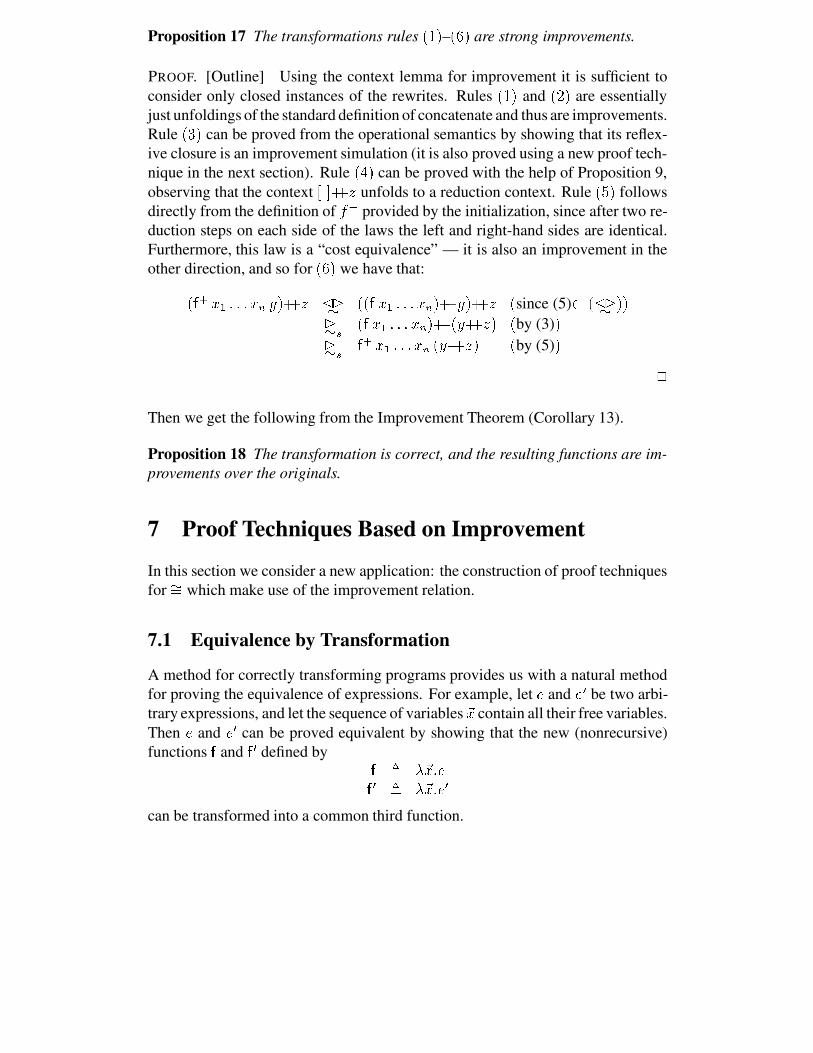
Proposition 17 The transformations rules 0$� 3 – 0 � 3 are strong improvements.

PROOF. [Outline] Using the context lemma for improvement it is sufficient toconsider only closed instances of the rewrites. Rules 0;� 3 and 0 ä 3 are essentiallyjust unfoldings of the standard definition of concatenate and thus are improvements.Rule 0�� 3 can be proved from the operational semantics by showing that its reflex-ive closure is an improvement simulation (it is also proved using a new proof tech-nique in the next section). Rule 0�� 3 can be proved with the help of Proposition 9,observing that the context

D9E ÅÅ&� unfolds to a reduction context. Rule 0-÷ 3 followsdirectly from the definition of � g provided by the initialization, since after two re-duction steps on each side of the laws the left and right-hand sides are identical.Furthermore, this law is a “cost equivalence” — it is also an improvement in theother direction, and so for 0 � 3 we have that:0 � g � � ��$� , � 3 ÅÅ&� y t` 0;0 � � � ��£� , 3 ÅÅB� 3 ÅÅ&� 0 since (5) ��0;y t` 3;3t`Jw 0 � � � �� , 3 ÅÅJ0-��ÅÅ&� 3 0 by (3) 3t`Jw � g � � ��;� , 0��9ÅÅ&� 3 0 by (5) 3 ¦Then we get the following from the Improvement Theorem (Corollary 13).

Proposition 18 The transformation is correct, and the resulting functions are im-provements over the originals.

7 Proof Techniques Based on Improvement

In this section we consider a new application: the construction of proof techniquesfor

` � which make use of the improvement relation.

7.1 Equivalence by Transformation

A method for correctly transforming programs provides us with a natural methodfor proving the equivalence of expressions. For example, let � and � ? be two arbi-trary expressions, and let the sequence of variables µ� contain all their free variables.Then � and �6? can be proved equivalent by showing that the new (nonrecursive)functions

�and

� ? defined by � �� µ�� ? �� µ�� 6?can be transformed into a common third function.


This approach to equivalence proofs was suggested by Kott (1982). Kott used avariant of the unfold-fold transformation method � to transform functions

�and

� ?into functions and ? respectively, such that and ? are syntactically identical upto renaming. Kott called this “the Mc Carthy method” after McCarthy’s recursioninduction principal (McCarthy 1967).

In this section we present a proof technique for equivalence which is derivedfrom this transformational viewpoint, using the improvement theorem. However,our method will abstract away from the transformational origins of the approach.The method will not explicitly construct functions like

�and

� ? above—except inthe correctness proof of the method itself.

7.2 Strong Improvement Up To Context

We introduce some notation to simplify the presentation. Let t denote a refinementof strong improvement given by� t � ? � + �>t`xw ¨ � ? �Definition 19 If P is a binary relation on expressions, let P C denote the closureunder substitution and context of P , given by7 0ãC D �� @ � ��W� � , @ , E �6C D � ? � @ � ��6� � ?, @ , E � � Z�P � ?Z �� KG��£i 8 �where C denotes an arbitrary i -holed context, and the @�Z are arbitrary substitu-tions.

Definition 20 (bisimulation up to improvement and context) A binary relationon expressions P is a bisimulation up to improvement and context if

whenever � � P � � , then there exists expressions � ? � and � ? � such that� � t � ? � � � � t � ? � � and � ? � P C � ? � �Theorem 5 If P is a bisimulation up to improvement and context, then P � ` � .

PROOF. Let P � 7 0 � Z¤� �6?Z 3 8 Z�ý^þ . Then by definition of improvement context sim-ulation, for each �vK�O there exist contexts CíZ , �ÕKùO such that � Z t C Z D µ� E and�6?Z t C Z D µ�S? E where where the respective pairs of expressions from µ� and µ�Ö? are sub-stitution instances of pairs in P . To simplify the exposition, assume that the C�Z�

Unfortunately, in (Kott 1982) the proposed method of ensuring that the unfold-fold transforma-tions are correct is unsound. Kott states (Proposition 1, loc. cit.) that unfold-fold transformationsfor a first-order call-by-value language are correct whenever the number of folds does not exceedthe number of unfolds. A counterexample can be found in Sands (1996b)(Section 1). Kott’s over-sight is that the language in question contains a non-strict operator—the conditional. Without thisoperator the Proposition is sound, but is not useful.

26 Sands

have only one distinct type of hole. The generalisation of the proof to the case of“polyadic” contexts is completely straightforward, but notationally cumbersome.

So for each 0 � Z�� W?Z 3 K P we have a substitution @�Z such that � Z t C Z D � ïã@[Z E and�W?Z t C Z D �W?ï @�Z E for some ðóK×O . Thus we define the following set of functions:Í � Z �� µ��Z-� C Z D � ï$@�Z E ��Z �� µ��Z-� C Z D � ?ï @�Z E �� Z t C Z D � ï$@�Z E �Øµ��Z � FV 0 � Z�C Z D � ï£@[Z E �W?Z C Z D �W?ï @�Z E 3�W?Z t C Z D �W?ï @�Z E �

Since t � ` � , we have that � Z `� C Z D � ï$@�Z E and �6?Z ` � C Z D �W?ï @[Z E . Hence it is sufficientto prove that

� Z `� RZ , ��KGO . We will do this by showing that the� Z and the �Z can be

correctly transformed, respectively, into functions� ?Z and ?Z such that

� ?Z and ?Z aresyntactically identical.

From the above definitions is easy to see that, for each ¢vK×O� e t`xw ¨ Che D �� @�e E for some ÒsKGOy t` � eYµ��eThus we have CÝZ D � ï£@[Z E t` w C Z D 0 � ïhµ�9ï 3 @�Z E . Using this fact together with The Improve-ment Theorem (viz. Corollary 13) we have that

� Z t` w � ?Z where� ?Z �� µ��ZV�®C Z D 0 � ?ï µ�9ï 3 @�Z E �Following the same lines we can show that QZ t`xw ?Z where ?Z �� µ� Z �®C Z D 0ô ?ï µ� ï 3 @ Z E �Since these function definitions are identical modulo naming, clearly we have

� Z t`>w� ?Z y t` ?Z and �Z t`>w ?Z . Since operational equivalence is contained in strict improve-ment, this concludes the proof. ¦Taking the special case of bisimulation up to improvement and contextwhich con-tains just a single pair of expressions (and where the context is unary), we obtain:

Corollary 21 Expressions � and ��? are operationally equivalent if there exists somecontext C , and some substitution @ such that� t C D � @ E and � ? t C D � ? @ EWe mention this special case because it turns out to be sufficient for many examples.The following variation of the above Theorem enables us to prove strong improve-ment properties:

Definition 22 (strong improvement up to improvement and context) A binaryrelation on expressions P is a strong improvement up to improvement and con-text if whenever �R� P �� , then there exists expressions � ? � and � ? � such that�� t � ? � � �� y t` ¨ � ? � � and � ? � P C � ? � �


Proposition 23 If P is a strong improvement up to improvement and context thenP � t`Jw .PROOF. (Sketch) As in the proof of Theorem 5, except that we obtain �1?Z y t` �ZNy t` ?Z , by making use of Proposition 14. ¦There are many other obvious variations of these proof methods along similar lines;for example for proving weaker properties like operational approximation 0 _` 3 andimprovement 0 t` 3 .7.3 Examples

Here we consider a few simple examples to illustrate the application of the prooftechniques given above. Corollary 21 will in fact be sufficient for current purposes.We will routinely omit simple calculations where they only employ the rules of thetick algebra.

Definition 2 A context C is a pseudo reduction context if it is a single-holed con-text which does not capture variables, and which satisfies the following properties:

1. C D ¨ � E y t` ¨ C D � E2. C D �!�";# �6< % � 4){ Ô � + �1� ��-4){ Ô , + � , E y t` �!�";# �W< % � 4�{QÔ � + C D �� E ��4�{QÔ , + C D � , E � FV 0ãC 3 distinct from FV 0�4�{QÔãZ 3

In what follows, we state that certain contexts are pseudo reduction contexts byway of a proof hint. To establish this property in all cases below requires nothingmore than the tick algebra, together with Proposition 9 (the propagation-rule forreduction contexts).

Associativity of Append We can prove the well-known associativity property ofappend by simply showing that P � 7 0;0-��ÅÅY� 3 ÅÅ&��ÅÅ>0-��ÅÅ&� 3;3 8 is a bisimulationup to improvement and context. In fact, in Section 6 we used a stronger property ofthe pair above, namely that it is contained in strong improvement. This is shown byproving that P is a strong improvement up to improvement and context. Contextsof the form

D�E ÅÅ � are pseudo reduction context, and using this fact the followingcalculations are routine:0��ÅÅB� 3 ÅÅ&� t`xw ¨ �!�";#Y� % �½�ª Ç + �9ÅÅ&��=�Ô + �Ó=)0 0¤Ô$ÅÅ&� 3 ÅÅ&� 3

��ÅÅJ0-��ÅÅ&� 3 y t` ¨ �!�";#Y� % �½�ª Ç + �9ÅÅ&��=�Ô + �Ó=)0 Ô$ÅÅ>0-��ÅÅ&� 3 3

28 Sands

The subexpressions are boxed to highlight the common context. The two boxedsubexpressions are just renamings of the respective expressions on the left-handsides. This is sufficient to show that P is a strong improvement up to improvementand context, and hence that 0��°ÅÅ&� 3 ÅÅ&� t`Jw �°ÅÅ>0��9ÅÅ&� 3 .

The example can, of course, be proved by considering all closed instances, andusing coinduction. The points to note are that the proof works directly on openexpressions, and that the “commmon context” (the expression “outside” the boxesabove) does indeed capture variables.

A Filter Example Continuing with standard examples, consider ¼ !�û and ��Ç © # ºdefined by:

�SÇ © # º ��R4�� ÑQ� �!�";#Y��Ñ % �½�ª Ç + ½�ª Ç��=Q��Ñ +ª � 4&� © ��# ½ ��=��SÇ © # º 4Þ��Ñ#RÇ "$#��Ç © # º 4ó�9Ñ

¼ !�û �� )r � �)�°ÑQ� �!�"$#Y�°Ñ % �½�ª Ç + ½�ª Ç�|=��9Ñ + 0-�J� 3 = ¼ !�ûJ�v�9ÑNow we wish to prove that� � ¼ !�û±�s0��Ç © # º 0�4¿Áö� 3 ��Ñ 3 ` � 0��Ç © # º 4>0 ¼ !�û �J��Ñ 3 � � ?where 0�4YÁ�� 3 is just shorthand for ��{��0Â4>0-�J{ 3;3 , (and where the conditional expres-sion in the definition of �SÇ © # º represents the obvious case-expression on booleans).We can do this by finding a context C , and a substitution @ such that � t C D � @ E and�W? t C D �W? @ E � Observing that �SÇ © # º � D�E and ¼ !�û±� D�E are pseudo reduction contexts,two simple calculations are sufficient to derive a suitable C and @ , namely:@ � 7 ��ÑÝ= � ��Ñ 8 and C � �!�";#Y��Ñ % �½�ª Ç + ½�ª Ç�|=��Ñ + ª � 4>0��¿� 3�© ��# ½ �§�Þ= DsE#�Ç ";# D�E �Equivalence of Fixed Point Combinators The previous examples can also beproved using more standard variations of “applicative bisimulation” (e.g., see Gor-don (1995)). The following example proves a property for which the usual bisimulation-like techniques are rather ineffective. The problem is to prove the equivalence oftwo different fixed point combinators. Define the following:� �� )��¡��0��J0�� 3;3� �� )��®�)��¡��0-�Y� 3

and as before, �9¹ �� )��¡��0��¹ � 3We can prove that

� `� ��¹ by constructing a bisimulation up to improvement andcontextwhich contains the above pair of expressions. As in the previous examples,


a relation which contains only this pair is sufficient. We begin with�

:� y t` ¨ �)��¡�J0��§0�� 3$3y t` ¨ �)��¡� ¨ 0��§0��ü�J0�� 3;3$3y t` ¨ �)��¡�J0 � � 3

From the definition of ��¹ we have immediately that �9¹Õy t` ¨ �)�Ö�Ã��0 ��¹ � 3 , and weare done. By two applications of Proposition 23 we also have that

� y t` ��¹ . Notethat if we had started with

� ? �� )��J0�� 3 we would not have been able to pro-ceed as above; but in this case

� ?St`Jw � follows by just unfolding � once.

7.4 Related Proof Techniques

We have used the terminology of “bisimulation up to” from CCS (see e.g., (Milner1989)). The closest proof technique to that presented here is Sangiorgi’s “weakbisimulation up-to context and up to expansion” which we discuss below.

Functional Proof Methods In the setting of functional languages Gordon (1995)has considered a number of variations on the basic Abramsky-style applicative bisim-ulation, including some “small step” versions. The method of bisimulation up toimprovement and contextintroduced here is sufficiently strong to prove all the ex-amples from (Gordon 1995) which hold in an untyped language � , and many of theproofs become simpler, and are certainly more calculational in style. AlthoughGordon’s methods are “complete” in theory, in practice one must be able to writedown representations of the bisimulations in question; it does not seem possible towrite down an appropriate bisimulation to prove ��¹ ` � �

without judicious quan-tification over contexts.

Pitts (Pitts 1995) has considered a variation of “bisimulation up to context” wheretwo expressions are bisimilar up to context if they both evaluate to weak head nor-mal forms with the same outermost constructor (or they both diverge), and the re-spective terms under the constructor can be obtained by substituting bisimilar termsinto a common subexpression. The weakness of Pitt’s method is that the “context”in question cannot capture variables.

Process Calculus Proof Methods The proof methods described in this sectionwere derived from the improvement theorem. However, there turns out to be a veryclosely related proof technique developed by Sangiorgi for the pi-calculus. Thisrelationship has influenced the terminology we have chosen.

In Sands (1991) we noted the similarity between the definition of improvement,and the efficiency preorder for CCS investigated by Arun-Kumar and Hennessy�

The operational equivalence in this paper is different from Gordon’s because his language isstatically typed, and because we observe termination of functions. The only example equivalencefrom (Gordon 1995) which does not hold here is the “Take Lemma”.

30 Sands

(Arun-Kumar and Hennessy 1991). The efficiency preorder is based on the numberof internal (silent) actions performed by a process, and expressed as a refinementof weak bisimulation. As with improvement, the application of the efficiency pre-order to the problem of reasoning about “ordinary” equivalence (in the case of CCS,weak bisimulation) seems to have come later; in (Sangiorgi and Milner 1992) theefficiency preorder, also dubbed expansion, is used to provide a “bisimulation upto” proof technique for weak bisimulation.

In the setting of the pi-calculus, Sangiorgi (1995, 1994) has used a refinement ofthese earlier proof techniques to great effect in studying the relationships betweenvarious calculi. The proof technique in question is called “bisimulation up to con-text and up to �` ”, where �` is the expansion relation. We will not go into the detailsof this proof technique here, but it contains similar ingredients to our bisimulationup to improvement and context. There are also some important differences. Weuse the t relation as an abstract alternative to using the one-step evaluation rela-tion. This enables us to handle open expressions, but the proof technique fails tobe complete (for example, it cannot prove that any pair of weak head normal formsare equivalent).

We summarise some informal correspondences between the notions in processcalculus and the relations defined in this article in Table 1. Our attempts to completethis picture find a more exact correspondence between the proof techniques relatingto bisimulation up to improvement and contexthave so far been unsuccessful.

Proces Calc. Functionalsilent transition ( �U ) bTU \ aTU bTU \strong bisimulation cost equivalence y t`weak bisimulation operational equivalence (

`� ) (see Gordon (1995))expansion ( �` ) strong improvement ( tùw )( �U �` ) strict improvement ( t )

Table 1: Informal relationships to Notions in Process Algebra

Another notion in concurrency which appears to have some connection to theImprovement Theorem, but which we have not yet investigated, is the metric-spacesemantics in the context of timed systems (e.g., Reed and Roscoe (1986)).

Acknowledgements Alan Jeffrey and Søren Lassen provided feedback on an ear-lier draft and made a number of valuable suggestions. The connections betweenproof techniques using the Improvement Theorem and Sangiorgi’s work which havebeen sketched in this article where discovered in collaboration with Davide San-giorgi. Thanks to Davide for numerous interesting discussions on the subject.


ReferencesAbramsky, S. (1990). The lazy lambda calculus. In D. Turner (Ed.), Research

Topics in Functional Programming, pp. 65–116. Reading, Mass.: Addison-Wesley.

Arun-Kumar, S. and M. Hennessy (1991). An efficiency preorder for processes.In TACS. LNCS 526.

Bird, R. and P. Wadler (1988). Introduction to Functional Programming. Pren-tice Hall.

Burstall, R. and J. Darlington (1977). A transformation system for developingrecursive programs. J. ACM 24(1), 44–67.

Courcelle, B. (1979). Infinite trees in normal form and recursive equations hav-ing a unique solution. Mathematical Systems Theory 13(1), 131–180.

Felleisen, M., D. Friedman, and E. Kohlbecker (1987). A syntactic theory ofsequential control. Theoretical Computer Science 52(1), 205–237.

Gordon, A. D. (1995). Bisimilarity as a theory of functional programming. Tech-nical Report BRICS NS-95-3, BRICS, Aarhus University, Denmark. Prelim-inary version in MFPS’95.

Howe, D. J. (1989). Equality in lazy computation systems. In The 4th AnnualSymposium on Logic in Computer Science, New York, pp. 198–203. IEEE.

Jones, N. D., C. Gomard, and P. Sestoft (1993). Partial Evaluation and Auto-matic Program Generation. Englewood Cliffs, N.J.: Prentice-Hall.

Kott, L. (1978). About transformation system: A theoretical study. In B. Robinet(Ed.), Program Transformations, Paris, pp. 232–247. Dunod.

Kott, L. (1982). The Mc Carthy’s recursion induction principle: “oldy” but“goody”. Calcolo 19(1), 59–69.

McCarthy, J. (1967). A Basis for a Mathematical Theory of Computation. Am-sterdam: North-Holland.

Milner, R. (1977). Fully abstract models of the typed lambda-calculus. Theoret-ical Computer Science 4(1), 1–22.

Milner, R. (1989). Communication and Concurrency. Englewwood Cliffs, N.J.:Prentice-Hall.

Pettorossi, A. and M. Proietti (1995). Rules and strategies for transformingfunctional and logic programs. To appear ACM Computing Surveys. (Pre-liminary version in Formal Program Development, LNCS 755, Springer-Verlag).

Peyton Jones, S. L. (1987). The Implementation of Functional ProgrammingLanguages. Prentice-Hall International Ltd. London.

32 Sands

Pitts, A. M. (1995, March). An extension of Howe’s “ 0�� 3 \ ” construction to yeildsimulation-up-to-context results. Unpublished Manuscript, Cambridge.

Plotkin, G. D. (1975). Call-by-name, Call-by-value and the � -calculus. Theoret-ical Computer Science 1(1), 125–159.

Reed, G. and A. Roscoe (1986). Metric space models for real-time concurrency.In ICALP’86, Volume 298 of LNCS. Springer-Verlag.

Sands, D. (1990). Calculi for Time Analysis of Functional Programs. Ph. D. the-sis, Dept. of Computing, Imperial College, Univ. of London, London.

Sands, D. (1991). Operational theories of improvement in functional languages(extended abstract). In Proceedings of the 4th Glasgow Workshop on Func-tional Programming (Skye, Scotland), pp. 298–311. Springer-Verlag.

Sands, D. (1993). A naıve time analysis and its theory of cost equivalence.TOPPS Rep. D-173, DIKU. Also in Logic and Comput., 5, 4, pp 495-541,1995.

Sands, D. (1995a). Higher-order expression procedures. In Proceeding of theACM SIGPLAN Syposium on Partial Evaluation and Semantics-Based Pro-gram Manipulation, PEPM’95, New York, pp. 190–201. ACM.

Sands, D. (1995b). Total correctness by local improvement in program transfor-mation. In POPL ’95. ACM Press. Extended version in (Sands 1996b).

Sands, D. (1996a). Proving the correctness of recursion-based automatic pro-gram transformations. Theoretical Computer Science A(167), xxx–xxx. Toappear. Preliminary version in TAPSOFT’95, LNCS 915.

Sands, D. (1996b). Total correctness by local improvement in the transformationof functional programs. ACM Transactions on Programming Languages andSystems (TOPLAS) 18(2), 175–234.

Sangiorgi, D. (1994). Locality and non-interleaving semantics in calculi for mo-bile processes. Technical report, LFCS, University of Edinburgh, Edinburgh,U.K.

Sangiorgi, D. (1995). Lazy functions and mobile processes. Rapport derecherche 2515, INRIA Sophia Antipolis.

Sangiorgi, D. and R. Milner (1992). The problem of "weak bisimulation up to".In Proceedings of CONCUR ’92, Number 789 in Lecture Notes in ComputerScience. Springer-Verlag.

Wadler, P. (1989). The concatenate vanishes. Univ. of Glasgow, Glasgow, Scot-land. Preliminary version circulated on the fp mailing list, 1987.

Wadler, P. (1990). Deforestation: Transforming programs to eliminate trees.Theoretical Computer Science 73(1), 231–248. Preliminary version in ESOP88, Lecture Notes in Computer Science, vol. 300.

Documents

Improvement Theory and its Applications - Chalmersdave/papers/hoots97.pdf · Improvement Theory and its Applications ... weak head normal forms. ... isfying the rules given in Figure