Improvement and spatial extension of the European Fish Indexefi-plus.boku.ac.at/downloads/Report_EFI-Medit_Final.pdf · 5 - To test new ecotaxa guilds for different types of pressures,

Project no.: 0044096

Project acronym: EFI+

Improvement and spatial extension of the European Fish Index

Instrument: STREP

Thematic Priority: Scientific Support to Policies (SSP) - POLICIES-1.5

Work Package 3, Subtask 7

Mediterranean River Assessment

Testing the response of guild-based metric

Final report December 2008

P. Segurado, M. T. Ferreira, P. Pinheiro & J. M. Santos

Instituto Superior de Agronomia, Portugal

December 2008

2

Table of contents

1. Introduction............................................................................................................................. 3 2. Definition of Mediterranean boundaries ................................................................................. 5

2.1 Background ...................................................................................................................... 5 2.2 The EFI+ classification ..................................................................................................... 6

3. Testing metrics’ response to pressure ................................................................................... 9 3.1 Environmental/explanatory variables ............................................................................... 9

3.1.1 Environmental variables included in the analyses..................................................... 9 3.1.2 Latent geomorphological variables............................................................................ 9

3.2 Pressures ....................................................................................................................... 11 3.2.1 Combined pressures ............................................................................................... 11 3.2.2 Relationships among single pressures.................................................................... 13 3.2.3 Relationships between environmental and pressure variables ............................... 15

3.3 Functional metrics considered........................................................................................ 18 3.4 Screening of fish data..................................................................................................... 20 3.5 Modelling metrics response to pressure......................................................................... 21

3.5.1 Overview.................................................................................................................. 21 3.5.2 Predictive modelling ................................................................................................ 22 3.5.3 Score computation................................................................................................... 22 3.5.4 Calibration dataset definition ................................................................................... 23 3.5.5 Metrics selection...................................................................................................... 26 3.5.5.1 Criteria and procedure.......................................................................................... 26 3.5.5.2 Scoring of metrics................................................................................................. 27 3.5.5.3 Selected candidate metrics .................................................................................. 37 a) Richness of adult insectivorous species (adult trophic guild) ....................................... 37 b) Richness of resident species (Migration guild) ............................................................. 42 c) Richness of potamodromous species (Migration guild) ................................................ 48 d) Richness of rheophilic spawning species (spawning habitat guild) .............................. 54 e) Richness of lithophilic spawning species (spawning substrate guild) .......................... 60 3.5.5.4 Summary of metrics’ response to pressure .......................................................... 66

4. Quantification of species tolerance values ........................................................................... 68 4.1 Data................................................................................................................................ 68 4.2 Statistical analyses......................................................................................................... 70 4.3 Estimated tolerances...................................................................................................... 72 4.3 Tolerance values versus expert judgment...................................................................... 78

5. Conclusions.......................................................................................................................... 79 6. References ........................................................................................................................... 82

3

1. Introduction Previously in FAME project and also in other studies, fish assemblage’ metric responses to

perturbation across Mediterranean areas were consistently weaker than those found for Central

and Temperate Europe (Pont et al. 2006; Schmutz et al. 2007). Major bottlenecks for the

development of a multimetric index in Mediterranean regions include i) a typical low species

richness per site, ii) a high degree of endemicity and basin-specific taxa assemblages; iii) the

naturally harsh and fluctuating, warm climate-dependent, aquatic environment, and iv) a complex

and hardly-predictable combination of hydrological variability with human pressures, either

present or inherited throughout centuries of fluvial and landscape uses. Moreover, there are also

considerable within-region differences related to the micro-scale fluctuating environments and

macroscale landscape patchiness, shaped by a complex geological evolutionary background.

Attempts to develop local metric indices for the Mediterranean regions dealt with these limitations

(Ferreira et al. 1996; Oliveira & Ferreira 2002; Magalhães et al. 2008), with modest degrees of

success and always at small regional scales, while taxa-based fish indices for quality assessment

are virtually non-existent.

Mediterranean-type regions generally experience limited water availability during part of the year.

For 6000 years now, Man has overcome this water shortage by building of reservoirs, water

abstraction from ground and surface sources and water transfers (Davies et al. 1994). In

temperate European rivers, anthropogenic disturbances are mostly related to water quality and

physical habitat modification, with hydrological alterations having only modest impacts. On the

other hand, in Mediterranean ecosystems the water quality deterioration is determined and

amplified by the amount (or lack) of water that flows in the river channel (in few cases

represented only by sewage water), and water quality is superimposed by the hydrological yearly

evolution. Even a small quantity of sewage can represent a large impairment when the river flow

is smaller than it should be, but likewise in can be masked if flow is artificially increased by dam or

irrigation outflows. The water quantity-dependent nature of human pressures results in less

predictable, antagonistic or cumulative effects. These effects have been taking place for

centuries, though intensified mid-last century onwards with the up-scale of engineering expertise

and materials. As a result, it is often difficult to determine whether a site is experiencing a natural

or otherwise induced flow change situation, or to quantify such change.

Hydrological variability of Mediterranean-type regions profoundly determines the life forms and life

cycles of aquatic organisms, as well as ecological processes (Gasith & Resh 1999). Fish fauna

from these heterogeneous ecosystems must frequently survive under alternating scenarios of too

much or too little water with a few intermediate but crucial periods of investment in recruitment

and growth. Under these conditions, fishes tend to have short life spans, rapid growth rates, high

4

fecundity and early sexual maturity and spawning, as well as generalist and opportunistic feeding

strategies (Granado-Lorencio 1996; Pires, Cowx & Coelho 2001; Vila-Gispert, Moreno-Amich &

Garcia-Berthou 2002). During low-flow season, biotic controls (e.g. predation, competition) may

take over assemblage responses to other pressures (Matthews & Marsh-Matthews 2003). The

apparent tolerance of native species to naturally harsh environments and their obvious short-term

resilience may actively mask man-made pressures, e.g. hinder the distinction between a

fortuitous series of natural low-flow years and the downstream water decrease through damming.

Clearly, the distinction of natural and human-induced disturbance is a central problem in

bioassessment (Fausch et al. 1990).

Finally, a further challenge in the Mediterranean rivers is to define accurate eco-taxa or guilds. In

Southern European peninsular areas, the primary freshwater fish fauna is dominated by cyprinids

and is characterized by a low number of genera and a high number of species per genera

(Doadrio, 2001). The low species richness per site, a high degree of endemicity and the presence

of basin-specific taxa assemblages, are problematic for developing biotic indices (Miller et al.

1988; Moyle & Marchetti 1999). Often, Mediterranean fish species have restricted distributions,

being limited to particular river basins or even river types. Therefore, bioassessments based on

fish assemblages in the Mediterranean region depends even more strongly upon eco-taxa (or

guild) definition. Similar taxa occurring at distinct basins, often with a recent genesis in geological

terms, are likely to have analogous ecological requirements, but frequently there is a lack of

evidence for such assumption. Yet, metric development strongly relies on accurate guild

classification and reliable tolerance responses. For this reason, in the present work, as a

complement to the testing of metrics’ response to pressures, a first attempt was made to estimate

species tolerance using a quantitative approach. The main objective of this analysis was to

assess the accuracy of tolerance-based guild classification based on expert judgment.

The objectives of the sub-task 3.7 Mediterranean River Assessment, which will be dealt with

along this report, included:

a) For the improvement of the database:

- To identify truly Mediterranean-type sites and increase the number of fishing sites available for

data treatment;

- To increase the quality and decrease the spatial scale of the impairment drivers, especially

those related to hydrological and geo-morphological changes;

- To increase the quality of the reference conditions, through ecological data screening

b) For the improvement of metric response:

- To attempt the definition of synthetic variables for different types of pressure;

5

- To test new ecotaxa guilds for different types of pressures, and for combined effects and

response types, taking into account the environmental background;

c) For contributing to follow-up Task 4:

- Improvement of metrics used before, on the basis of the tolerance indicator’ values obtained in

this study, tolerant species and intolerant species;

- Recommendations of inclusion of Mediterranean-specific metrics and single or combined

pressures, to be used in Task 4;

- Recommendations to be incorporated in the development of the EFI model.

2. Definition of Mediterranean boundaries

2.1 Background

The task of identifying Mediterranean-type rivers at the European scale is particularly challenging,

as no unequivocal and consensual criteria are found in the literature, even for classifying

Mediterranean climate zones (Hooke 2006). According to early definitions, such as those of

Köppen (Harding 2006; Hooke 2006), the Mediterranean region corresponds to the climatic zone

in which there is at least three times as much rain in the wettest month of winter as in the driest

month of summer, the latter having less than 30mm precipitation. However, this definition has the

limitation of only considering the temporal distribution of precipitation, which is not the single

factor influencing the hydrological regimes. Other climatic parameters such as temperature and

evapotranspiration also play an important role on water availability along the year.

More recent bioclimatic classification criteria, mainly those developed by Rivas-Martinez (1999;

2005), take into account the annual distribution and relationships among several climatic

parameters. One of the most important parameters are the Ombrothermic Indexes that, in broad

terms, are given by the quotient between Precipitation and Temperature, though they may

express slightly different conditions depending on how they are calculated (see Rivas-Martinez

1999 for further details on index calculations). According to the Rivas-Martinez ombrothermic

criteria, the Mediterranean macrobioclimate is characterized by, at least, two consecutive dry

months during the summer. A month is defined as dry if the precipitation (mm) is less than twice

the temperature (centigrade degrees). Hence, if the ombrothermic bimonthly quotient of the two

driest months is higher than two, the territory is not Mediterranean. However, if that quotient is

less than two, the territory may or may not be Mediterranean, as the bimonthly deficient hydrical

balance may or may not compensated with the previous month’s precipitation. To account for this

6

compensatory effect a table of Summer ombrothermic compensation values was defined (see

Rivas-Martinez 1999, for further details).

The task of defining Mediterranean regions is even more demanding when we consider the high

variability of annual precipitation among Mediterranean areas. Rainfall usually ranges between

275 and 900 mm, but certain Mediterranean-climate regions may fall into the category of semiarid

regions, i.e., with annual precipitation ranging between 200 and 500 mm (Velasco et al. 2003).

Despite the absence of consistent and simple criteria, there are four basic characteristics of

Mediterranean climate that are most often mentioned in the literature, namely i) low annual

precipitation, ii) high precipitation seasonality, iii) mild winters and iv) hot and dry summers (e.g.

Blondel & Aronson 1999; Gasith & Resh 1999; Hooker 2006). As a consequence, streams on this

climatic region have two important features that makes them diverge from other European rivers:

i) the frequent occurrence of extreme flood or torrential events due to the concentration of annual

precipitation in few months and ii) the occurrence of a dry period, during which the water flow is

interrupted, due to very low rainfall and high temperatures on summer months (Romero et al.

1998; Gasith & Resh 1999; Magalhães et al. 2002; Bonada et al. 2005; Ferreira et al. 2007a).

Among the climatic attributes typically attributed to Mediterranean regions, we intentionally

favoured those that affect more directly the extent of the dry season. In fact, it is here assumed

that these attributes are the most closely related to a key feature of Mediterranean streams that

have strong implications on bioassessment analyses: the increased role of spatial pattern and

physical characteristics of summer refugia on structuring fish assemblages (Magalhães et al.,

2002).

2.2 The EFI+ classification

In our identification of Mediterranean sites, given the great number of sites and the extent of

territory to be classified, we have used exclusively climatic information, mainly for its availability

and simplicity to process in a GIS environment.

With the purpose of express in a simple and straightforward way the probability of a given river

stretch to show Mediterranean features we based our classification on relationships between

temperature and precipitation only. Information on these two parameters has the advantage of

being easily available over a vast territory and with adequate spatial and temporal resolutions.

We adopted a conservative criteria of mediterranity by considering the fourmonthly estival

ombrothermic index (Ios4), that is, the sum of monthly precipitation divided by the sum of monthly

mean temperature of the two driest months (July and August in Europe) plus the two previous

months (May and June):

7

104 ×++++++

=AugustJulyJuneMay

AugustJulyJuneMay

TpTpTpTpPpPpPpPp

Ios Eq. 1

, where Ppm and Tpm are, respectively, the yearly positive precipitation (in mm, total average

precipitation of those months whose average temperature is higher than 0ºC) and the yearly

positive temperature (in tenths of degrees Celsius, sum of the monthly average temperature of

those months whose average temperature is higher than 0ºC) on month m. The two months prior

to the dry period are included because it is assumed that summer aridity greatly depends on the

rain that falls during May and June.

Since this criteria included many regions from the Atlantic climatic zone we further use a total

annual precipitation (TAP) threshold of 1200 mm to separate Mediterranean from temperate

regions. We considered two levels of mediterranity according to the following criteria:

Mediterranity level 1 - Ios4 < 1 AND TAP < 1200mm

Mediterranity level 2 - Ios4 < 2 AND TAP < 1200mm

As climatic variables we used 30 seconds (600 - 800 meters) resolution maps of monthly

precipitation and monthly mean temperature that are freely available in the WORLDCLIM website

(http://www.worldclim.org/).

According to the resulting map (Fig. 1) the level 1 Mediterranean zone, among the countries of

the EFI+ consortium, include most of the Iberian Peninsula, the Southern France coastal strip and

Southern Italy. The level 2 Mediterranean zone mainly represent an extension to more continental

zones. The map of figure 1 also shows some isolated areas (e.g. in Loire, France, central

Hungary and eastern Romania) classified as level 2 Mediterranean zone. Sites included in those

areas were not included in the mediterranean river dataset.

8

Fig. 1 – EFI+ classification of Mediterranity across Europe.

According to the chosen classification, Spain is the country with the largest Mediterranean area,

followed by Italy, Portugal and France (Table 1). Spain has also the highest total number of sites,

followed by Portugal, Italy and France (Table 1, Fig. 2). However, the number of sites in Spain is

not representative of the area covered by each bioclimatic zone. For example, the level 1

mediterranean zone is clearly under-represented in Spanish dataset.

Table 1 – Total area (106 ha) of each bioclimatic region and number of Mediterranean sites per country.

Bioclimatic zone Italy France Spain Portugal

Temperate 12.19 49.82 10.46 1.14

Mediterranean level 1 11.63 1.47 29.60 6.91 Area

Mediterranean level2 6.48 3.49 9.29 0.85

Temperate 461 1051 1791 105

Mediterranean level 1 51 20 1092 721

Mediterranean level2 140 74 1356 97 Number of sites

Total 652 1145 4239 923

9

Fig. 2 – Location of Mediterranean river EFI+ sites.

3. Testing metrics’ response to pressure

3.1 Environmental/explanatory variables

3.1.1 Environmental variables included in the analyses

Twelve environmental variables were considered, partially based on those used in WP4: two

climatic (mean temperature in July and thermal amplitude – difference between mean

temperature in January and July), one hydrological (flow regime), two topographical (altitude and

river slope), two geological (geological typology and natural sediment) and five geomorphological

variables (geomorphologic river type, valley form, floodplain, distance to source and catchment

area). Variables “actual river slope”, “distance to source” and “catchment area” were log-

transformed.

3.1.2 Latent geomorphological variables

Following the same procedure used in WP4, in order to get latent variables that describe in few

dimensions the river types, an ordination method was used to summarise geomorphological

information. A generalisation of the Hill-Smith ordination method was used (Hill & Smith 1976)

that deals with mixed type variables (quantitative, factor and ordered). The mixed analysis was

10

run using the dudi.mix function (Dray & Dufour 2007) of the Ade4 package (Thioulouse et al.

1997) for R version 7.0.1 (R Development Core Team 2007).

The first axis of the resulting multivariate analysis is mainly related to variations in

geomorphologic river types (Fig. 3, table 2). This axis is positively related with braided rivers,

distance to source, catchment area, presence of former floodplains and plain-shape valley

(longitudinal gradient). The second axis also describes a longitudinal river gradient but is mainly

related to valley form, with a strong positive relationship with U-shape valley types and a negative

relationship with plain-shape valley.

Fig. 3 – Biplot of the mixed analysis using geomorphological data.

11

Table 2 – Geomorphological variable scores of mixed analysis.

Variables Axis 1 Axis 2

Geomorphological type - Braided 1.59 -0.77

Geomorphological type - Constraint -0.27 0.19

Geomorphological type - Meandrous 0.36 0.47

Geomorphological type - Sinuous -0.06 -0.08

Log Distance to source 0.52 0.41

Log Catchment area 0.53 0.41

Former floodplain - No -0.24 0.29

Former floodplain - Yes 0.78 -0.95

Valley form - Plains 0.77 -0.91

Valley form - U-shape 0.26 2.28

Vally form - V-shape -0.26 0.24

3.2 Pressures

3.2.1 Combined pressures

The selected single pressure variables were integrated into synthetic pressure variables

according both to pressure-type-specific combinations and a global pressure combination. We

used the scores of the first component of Principal Component Analysis as combined variables, in

order to account for colinearities among variables. The PCA were carried out using R version

7.0.1 (R Development Core Team 2007), based on the correlation matrix.

Four pressure-type-specific combinations were therefore obtained expressing, respectively,

problems of connectivity, hydrology, morphology and water quality. Two global pressure

combinations were also considered either including or excluding connectivity-related pressures.

The PCA scores were rescaled between 0 and 1 and log transformed. The selected single

pressure variables, their classification scheme and the correspondent pressure types are shown

in table 3.

12

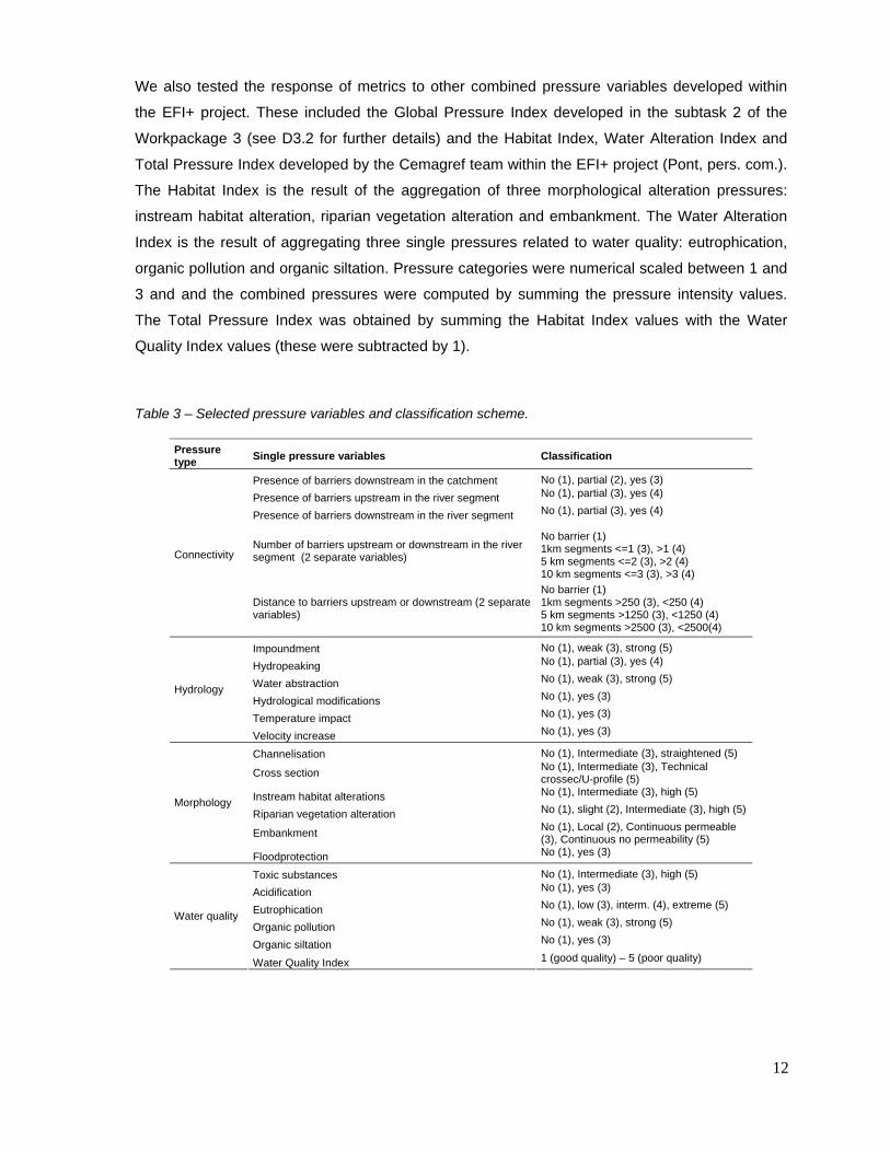
We also tested the response of metrics to other combined pressure variables developed within

the EFI+ project. These included the Global Pressure Index developed in the subtask 2 of the

Workpackage 3 (see D3.2 for further details) and the Habitat Index, Water Alteration Index and

Total Pressure Index developed by the Cemagref team within the EFI+ project (Pont, pers. com.).

The Habitat Index is the result of the aggregation of three morphological alteration pressures:

instream habitat alteration, riparian vegetation alteration and embankment. The Water Alteration

Index is the result of aggregating three single pressures related to water quality: eutrophication,

organic pollution and organic siltation. Pressure categories were numerical scaled between 1 and

3 and and the combined pressures were computed by summing the pressure intensity values.

The Total Pressure Index was obtained by summing the Habitat Index values with the Water

Quality Index values (these were subtracted by 1).

Table 3 – Selected pressure variables and classification scheme.

Pressure type Single pressure variables Classification

Presence of barriers downstream in the catchment No (1), partial (2), yes (3) Presence of barriers upstream in the river segment No (1), partial (3), yes (4)

Presence of barriers downstream in the river segment No (1), partial (3), yes (4)

Number of barriers upstream or downstream in the river segment (2 separate variables)

No barrier (1) 1km segments <=1 (3), >1 (4) 5 km segments <=2 (3), >2 (4) 10 km segments <=3 (3), >3 (4)

Connectivity

Distance to barriers upstream or downstream (2 separate variables)

No barrier (1) 1km segments >250 (3), <250 (4) 5 km segments >1250 (3), <1250 (4) 10 km segments >2500 (3), <2500(4)

Impoundment No (1), weak (3), strong (5)

Hydropeaking No (1), partial (3), yes (4)

Water abstraction No (1), weak (3), strong (5)

Hydrological modifications No (1), yes (3)

Temperature impact No (1), yes (3)

Hydrology

Velocity increase No (1), yes (3)

Channelisation No (1), Intermediate (3), straightened (5)

Cross section No (1), Intermediate (3), Technical crossec/U-profile (5)

Instream habitat alterations No (1), Intermediate (3), high (5)

Riparian vegetation alteration No (1), slight (2), Intermediate (3), high (5)

Embankment No (1), Local (2), Continuous permeable (3), Continuous no permeability (5)

Morphology

Floodprotection No (1), yes (3)

Toxic substances No (1), Intermediate (3), high (5) Acidification No (1), yes (3)

Eutrophication No (1), low (3), interm. (4), extreme (5)

Organic pollution No (1), weak (3), strong (5)

Organic siltation No (1), yes (3)

Water quality

Water Quality Index 1 (good quality) – 5 (poor quality)

13

3.2.2 Relationships among single pressures

The main relationships among single pressures are represented in figure 4, showing the plot of

the pressure scores in the first plane of the PCA. The different pressure types are clearly

separated by the first PCA plane (Fig 4). The first axis explains 19% of the variance and is mainly

related to connectivity and hydrogical disturbances (Fig. 4, Table 4). The second axis explains

13% of the variance and essentially describes morphological disturbances. Water quality-related

disturbances are comparatively more associated to morphological disturbances than to other

pressure types.

Fig. 4 – First plane of the pressure PCA.

14

Table 4 – Loadings of pressure variables in the first two axis of the pressure PCA.

variables CS1 CS2 Barriers_catchment_down 0.013 -0.250 Barriers_river_segment_up -0.300 -0.159 Barriers_river_segment_down -0.298 -0.183 Barriers_number_river_segment_up -0.300 -0.159 Barriers_number_river_segment_down -0.298 -0.183 Barriers_distance_river_segment_up -0.296 -0.162 Barriers_distance_river_segment_down -0.293 -0.184 Impoundment -0.311 -0.070 Hydropeaking -0.252 -0.040 Water_abstraction -0.198 0.034 Hydro_mod -0.275 -0.053 Temperature_impact -0.088 -0.121 Velocity_increase -0.123 0.363 Channelisation -0.159 0.357 Cross_sec -0.145 0.305 Instream_habitat -0.135 0.311 Riparian_vegetation -0.132 0.245 Embankment -0.123 0.214 Floodprotection -0.095 0.182 Toxic_substances -0.094 0.213 Acidification -0.007 0.000 Water_quality_index -0.135 0.183 Eutrophication -0.116 0.102 Organic_pollution -0.108 0.100 Organic_siltation -0.107 0.216

According to the sites scores of the first axis of the PCA computed separately for each type of

pressure and the whole set of pressures, there are some differences in the incidence of pressures

between the studied Mediterranean countries: 1) except for hydrological disturbances, French

sites shows a higher overall variability of pressure incidence between sites; 2) French and Italian

sites tend to show higher incidence of connectivity problems than Iberian countries; 3)

Portuguese sites show higher average hydrological disturbances and higher variability between

sites for this pressure type than the other countries; 4) Spanish and Italian sites show higher

problems of water quality; 5) Spanish sites tend to have an overall lower incidence of pressures.

15

3.2.3 Relationships between environmental and pressure variables

Aiming to explore relationships between environmental and pressure datasets we performed co-

inertia analysis (Dray et al. 2003) separately for each kind of pressure. The purpose of co-inertia

analysis is the matching of two data tables, usually a site-by-environmental variables table and a

Fig. 5 – Boxplots showing the

distribution of the normed scores of

the first PCA axis at each country

(PT – Portugal; ES – Spain, FR –

France, IT – Italy).

16

site-by-species table. Co-inertia aims to find a vector in the “species” space and a vector in the

“environmental” space with maximal co-inertia. The second and further pairs of vectors maximise

the same quantity but are subject to extra constraints of orthogonality (see Dray et al. 2003 for

further details on the method). The advantage of this method over other methods (e.g.

Redundancy Analysis and Canonical Correspondence Analysis) is that it allows linking two

hyperspaces from distinct ordination methods (for example Principal Component Analysis and

Correspondence Analysis). Co-inertia analysis was performed with the coinertia function (Dray et

al., 2007) of the Ade4 package (Thioulouse et al. 1997) for R version 7.0.1 (R Development Core

Team, 2007).

Here we used the site-by-environmental variables table, in the form of a Hill-Smith mix PCA (see

subsection 3.1), and the site-by-pressure table, in the form of a PCA (see subsection 3.2), to

explore and quantify the covariability between the environmental variability and each pressure-

type. This analysis was restricted to sites with no missing data for all environmental and pressure

variables (670 sites).

The co-inertia analysis using the whole set of single pressures shows a good agreement between

the first environmental and pressure co-inertia vectors (r = 0.72). The normed scores of variables

in the first environmental co-inertia plane (Table 5a) shows that the first environmental co-inertia

vector is mainly related to lowland rivers (braided geomorphological type, presence of former

floodplain and valley shape - plains), which means that the main covariation between

environmental and pressure variables is expressed mainly between lowland rivers and the

remaining river types. On the other hand, the second co-inertia vector is comparatively more

influenced by climate and variables that reflect more directly the longitudinal gradient (e.g.

distance to source and catchment area).

The normed scores of pressure variables in the first co-inertia plane (Table 5b) shows that the

two first vectors are greatly related to the existence of barriers downstream at the catchment level

(which, in fact, reflects the longitudinal river gradient). The first co-inertia axis is equally related to

hydrological, morphological and water quality disturbances while the second axis comparatively

more related to hydrological pressures.

17

Table 5 – Normed scores of environmental (a) and pressure variables in, respectively the first

environmental and pressure co-inertia planes (colour intensity is proportional to the absolute value

magnitude).

a) Variable type Environmental variables CS1 CS2

Geomophological type - Braided 2.20 0.02 Geomophological type - Constraint -0.19 0.07 Geomophological type - Meand 0.26 0.45 Geomophological type - Sinuous -0.05 -0.05 Log Distande to source 0.23 -0.53 Log Catchment area 0.29 -0.52 Former floodplain - No -0.13 -0.07 Former floodplain - Yes 0.72 0.42 Valley shape - Plains 0.83 0.43

Geomorphology

Valle shape - V-shape -0.15 -0.08 Flow regime - Permanent -0.03 -0.06 Hidrologic regime Flow regime - Summer_dry 0.07 0.12 Altitude -0.43 -0.04 Topography Log River slope -0.35 0.26 Geology - Calcareous -0.17 0.40 Geology - Siliceous 0.02 -0.04 Geology Natural sediment -0.27 -0.26 Mean Temperature in July 0.03 -0.22 Climate Thermal Amplitude (Tjul – T Jan) -0.41 -0.39

b) Pressure type Pressure variables RS1 RS2

Barriers_catchment_down -0.41 -0.38 Barriers_river_segment_up 0.03 -0.16 Barriers_river_segment_down 0.02 -0.15 Barriers_number_river_segment_up 0.03 -0.16 Barriers_number_river_segment_down 0.03 -0.18 Barriers_distance_river_segment_up 0.03 -0.15

Connectivity

Barriers_distance_river_segment_down 0.03 -0.18 Impoundment 0.15 -0.28 Hydropeaking 0.21 -0.43 Water_abstraction 0.23 -0.19 Hydro_mod 0.23 -0.38 Temperature_impact -0.02 -0.09

Hydrology

Velocity_increase 0.29 0.15 Channelisation 0.32 0.09 Cross_sec 0.26 0.14 Instream_habitat 0.23 0.19 Riparian_vegetation 0.17 0.12 Embankment 0.07 0.06

Morphology

Floodprotection 0.26 -0.07 Toxic_substances 0.18 -0.03 Acidification 0.03 0.04 Water_quality_index 0.28 0.14 Eutrophication 0.19 -0.30 Organic_pollution 0.18 -0.15

Water quality

Organic_siltation 0.27 0.09

18

3.3 Functional metrics considered

We tested the response of 118 functional metrics based on measures of diversity and abundance

and 19 guilds. These metrics were retained after eliminating those with less than 10 positive

cases in the dataset. Among these, sixteen new specific metrics for Mediterranean rivers, based

on the maximum size of native Mediterranean cyprinids, were tested: density/richness of

large/small cyprinids, density/richness of large/small cyprinids intolerant to habitat degradation,

density/richness of large/small cyprinids tolerant to habitat degradation, density/richness of

large/small cyprinids tolerant to habitat quality (Table 6). Large native cyprinids were defined as

those comprising length sizes higher or equal to 300mm (table 7). The remaining guilds included:

species richness, total density, species’ origin (native versus exotic), seven tolerance guilds

(general water quality, dissolved oxiden, toxic substances, acidification, habitat degradation,

clustering based on tolerance guilds - 3 groups, clustering based on tolerance guilds - 5 groups),

reproductive guild, habitat use, feeding habitat, adult trophic guild, spawning habitat preferences,

reproductive behaviour, parental care, migration guild, salinity tolerance, and two new guilds

(Table 6).

Table 6 – List of tested metrics and number of positive values

Guild Description Metrics’ ID N (positive)

Total Richness N_sp_All 646 Global

Total density Density_sp_All 646

Origin Native species Native 635

Intermediate HTOL_HIM 600

Intolerant HTOL_HINTOL 275 Habitat degradation tolerance tolerant HTOL_HTOL 494

Intermediate WQgen_IM 588

Intolerant WQgen_INTOL 224 General water quality tolerance tolerant WQgen_TOL 544

Intermediate WQAc_AIM 573

Intolerant WQAc_AINTOL 232 Acid tolerance

tolerant WQAc_ATOL 403

Intermediate WQO2_O2IM 596

Intolerant WQO2_O2INTOL 226 Water quality tolerance O2

tolerant WQO2_O2TOL 445

Intermediate WQTox_TOXIM 606

Intolerant WQTox_TOXINTOL 226 Water quality tolerance TOX

tolerant WQTox_TOXTOL 530

Intermediate CLU5_3_Intermediate 586

Intolerant CLU5_3_Intolerant 220

Cluster based on tolerance guilds - 3 groups tolerant CLU5_3_Tolerant 544

19

( cont.) Intolerant (level 1) CLU5_3b_Intol1 198

Intolerant (level 2) CLU5_3b_Intol2 96

Intermediate CLU5_3b_Medium 559

Tolerant (level 1) CLU5_3b_Tol1 236

Cluster based on tolerance guilds - 5 groups

Tolerant (level 2) CLU5_3b_Tol2 577

Detritivorous Atroph_DETR 364

Insectivorous Atroph_INSV 630 Adult trophic guild

Omnivorous Atroph_OMNI 518

Benthic FeHab_B 583 Feeding habitat

Water column FeHab_WC 637

Eurytopic Hab_EURY 602

Limnophilic Hab_LIMNO 405 Habitat

Rheophilic Hab_RH 449

Eurytopic HabSp_EUPAR 530

Limnophilic HabSp_LIPAR 357 Habitat spawning preferences Rheophilic HabSp_RHPAR 586

Long catadromous Mig_LONG_LMC 146

Potamodromous Mig_POTAD 561 Migration guild

Resident Mig_RESID 611

No protection PC_NOP 638 Parental care Protection (eggs

and/or larvae) PC_PROT 246

Lithophilic Repro_LITH 606

Pelagic Repro_PELA 148

Phyto-lithophilic Repro_PHLI 113

Phytophilic Repro_PHYT 238

Polyphilic Repro_POLY 317

Reproductive guild

psamnophilic Repro_PSAM 143 Fractional spawners ReproB_FR 436 Reproductive

behaviour Single spawners ReproB_SIN 624 Anadromous - catadromous Sal_ANCA 152

Salinity Freshwater Sal_FRE 645

Richness / Density cyp_L 520 Habitat degradation - intolerant cyp_L_HTOL_HINTOL 33

Habitat degradation - tolerant cyp_L_HTOL_HTOL 29

Large endemic cyprinids

Water quality general - tolerant cyp_L_WQgen_TOL 421

Richness / Density cyp_S 503 Habitat degradation - intolerant cyp_S_HTOL_HINTOL 96

Habitat degradation - tolerant cyp_S_HTOL_HTOL 279

Small endemic cyprinids

Water quality general - tolerant cyp_S_WQgen_TOL 174

20

Table 7 – Cyprinid guild classification according to the maximum body lengths (Large - > 300mm; Small - < 300mm).

Species_name Guild Species_name Guild Abramis brama Large Chondrostoma toxostoma Large Achondrostoma arcasii Small Chondrostoma turiense Large Achondrostoma occidentale Small Iberochondrostoma almacai Small Achondrostoma oligolepis Small Iberochondrostoma lemmingii Small Alburnoides bipunctatus Small Iberochondrostoma lusitanicum Small Alburnus albidus Small Leuciscus cephalus Large Alburnus alburnus Small Leuciscus leuciscus Large Anaecypris hispanica Small Leuciscus lucumonis Small Barbus barbus Large Leuciscus souffia Small Barbus bocagei Large Pachychilon pictum Small Barbus comizo Large Phoxinus phoxinus Small Barbus graellsii Large Pseudochondrostoma duriense Large Barbus guiraonis Large Pseudochondrostoma polylepis Large Barbus haasi Large Pseudochondrostoma willkommii Large Barbus meridionalis Small Rhodeus amarus Small Barbus microcephalus Large Rutilus aula Small Barbus plebejus Large Rutilus rubilio Small Barbus sclateri Large Rutilus rutilus Large Barbus tyberinus Large Squalius alburnoides Small Chondrostoma genei Large Squalius aradensis Small Chondrostoma miegii Small Squalius carolitertii Small Chondrostoma nasus Large Squalius pyrenaicus Small Chondrostoma soetta Large Squalius torgalensis Small

3.4 Screening of fish data

The criteria for the inclusion of sites in the Mediterranean dataset were the following:

• Only sites from level 1 mediterranean region were included; this option was based on the

fact that level 1 showed more distinctive features, both in terms of environmental and

pressure variables (e.g. Figs 6 - 8).

• Only the first run was considered for presence/absence and abundance estimates;

• Fishing occasions with fished area larger than 100m2;

• Fishing occasions with more than 50 individuals;

• Only sites with no missing data for the set of environmental variables considered in the

analysis;

• Large rivers (catchment size > 10 000 km2 and wetted width > 50 m) were not included.

21

• Regarding flow regime, both “permanent” and “summer dry” sites were included since in

the level 1 Mediterranean region the proportion of sites with “summer dry” flow regime is

much higher (Fig. 6) and, moreover, it is a key feature of Mediterranean streams.

Fig. 6 – Frequency of sites per class of flow regime (n = 14222 sites).

A total of 782 fishing occasions were preselected according to above criteria. Among each site

the fishing occasion with a greater total number of fish caught was selected, which resulted in a

total of 646 sites after the data screening (Fig. 9).

3.5 Modelling metrics response to pressure

3.5.1 Overview

The response of metrics to human induced pressures was tested after controlling for

environmental variability, using the EFI approach (Pont et al. 2006, 2007). In essence this

approach is based on the premise that metrics based on functional guilds are responsive to

environmental variability, such that it is possible to predict, with an acceptable accuracy, metrics

outcome through the use of statistical models. Statistical models relating each functional metrics

to a set of environmental predictors are first adjusted using exclusively a dataset comprising the

least disturbed sites (calibration dataset). The calibration model is then used to predict metrics

outcome for the remaining impaired sites and the difference between the observed and the

22

predicted metrics’ values (residuals) is assumed to be proportional to some kind of human

induced pressure. In this way it is possible to isolate the effect of human induced disturbances

from that of natural environmental variability. This approach has the advantage of being in total

conformity with the reference condition approach imposed by the Water Framework Directive

(WFD), since it provides a way of quantifying deviations from reference conditions. All statistical

analysis were performed using functions and routines implemented in R software version 2.7.1 (R

Development Core Team 2007).

3.5.2 Predictive modelling

A General Linear Modelling (GLM; McCullagh & Nelder, 1989) assuming a Poisson distribution of

errors and a log link function (i.e. Poisson regression) was used to determine the relationships

between each functional metric and the environmental variables. This method was both used for

metrics based on richness and metrics based on abundance. An offset term was associated to

the Poisson regression since there is a straight dependency between the number

individuals/species belonging to a certain guild and the total number of individuals/species. The

offset term was included in the regression equation as log(total number of species) for metric

based on richness and log(total number of individuals) for metric based on abundance. A

stepwise procedure based on Akaike Information Criterion (AIC) was used to select variables to

be included in models (StepAIC function of the MASS library for R; Venables & Ripley, 1997).

3.5.3 Score computation

The score computation was based on the procedure proposed by Pont et al. (2006; 2007) which

very briefly involves the following steps: 1) Computation of the predicted values for the non-

calibration dataset; 2) standardisation of the resulting residuals (observed – predicted) through

the subtraction and division by, respectively, the mean and the standard deviation of the residuals

obtained from models using calibration dataset (i.e., a distribution of residuals with mean zero and

standard deviation equal to one is obtained), 3) transformation of residuals into values ranging

from 0 to 1, which reflect the probability of a site being a reference site, by assuming that

residuals are normally distributed with mean and standard deviation equal, respectively, to zero

and one. The residual value transformation was performed using the pnorm(x) function in R which

computes the value of the cumulative normal distribution function that corresponds to the x value,

i.e., the probability of obtaining a value lower than the observed one. For those metrics that were

expected to be positively related to the intensity of human pressure the transformation used was

23

in the form 1-pnorm(x), while those metrics that were expected to have a unimodal relationship

with pressures the transformation was in the form 2*pnorm(-abs(x)).

3.5.4 Calibration dataset definition

The selection of Mediterranean sites to be used in model calibration was similar to that used for

the WP4, with the following adaptations to Mediterranean rivers:

• Eutrophication – the “intermediate” class was included since Mediterranean region

(namely from level 1) shows a much higher proportion of sites with “low” and

“intermediate” eutrophication (although it is uncertain how much of it is natural

eutrophication) (Fig. 7).

• Riparian vegetation – the “Intermediate” class was included in the calibration dataset,

since the proportion of Mediterranean sites with “low” and “intermediate” levels of riparian

vegetation degradation is much higher than for the non-mediterranean sites (Fig. 8);

furthermore, riparian naturalness can be easily confounded with “low” and “intermediate”

classes because vegetation in many cases is naturally reduced to small trees and shrubs.

• Sedimentation – this variable was dropped out as a criteria because there were too many

missing data in the Mediterranean region and data on natural sedimentation is virtually

non-existent.

• Velocity increase and temperature impact – these variables were dropped out as a criteria,

as the compilation of these variables is more subjective than other hydrological variables.

According to the criteria adopted in WP4 with the above adaptations (Table 8), a total of 112 sites

(Fig. 9) were available to calibrate models of metrics response to environmental variability. These

sites show a fairly good representation along the main environmental gradients according to the

scores of a mixed analysis (see 3.1 for some details on the method) using the whole set of

environmental variables considered (Fig. 10). This is specially true for the second mixed analysis

axis. According to the first axis, the scores of the calibration sites tend to be lower than those for

non-calibration data. However, the range of values for calibration sites is contained within the

range of values for non-calibration sites (Fig. 10).

24

Fig. 7 – Frequency of sites per class of eutrophication intensity (n = 14222 sites).

Fig. 8 – Frequency of sites per magnitude of riparian vegetation disturbance (n = 14222 sites).

25

Table 8 –Criteria for inclusion of sites on the Mediterranean calibration dataset (the sign ” |” means “or”).

• Barriers_river_segment_down == "No" | Barriers_river_segment_down == "Partial"

• Impoundment == "No"

• Hydropeaking == "No"

• Water abstraction == "No" | Water abstraction == "Weak"

• Hydro_mod == "No" | Hydro_mod == "NoData"

• Channelization == "No" | Channelization == "Intermediate"

• Cross_sec == "No"

• Instream_habitat == "No" | Instream_habitat == "Intermediate" | Instream_habitat == "NoData"

• Riparian vegetation == "No" | Riparian vegetation == "slight" | Riparian vegetation == "Intermediate" | Riparian

vegetation == "NoData"

• Embankment == "No" | Embankment == "Local" | Embankment == "NoData"

• Toxic substances == "No" | Toxic substances == "Intermediate" | Toxic substances == "NoData"

• Acidification == "No" | Acidification == "NoData"

• Water Quality Index == 1 | Water Quality Index == 2 | Water Quality Index == 3 (for Portugal only)

• Eutrophication == “No” | Eutrophication == “Low” | Eutrophication == “Intermediate” | Eutrophication ==

"NoData"

• Organic pollution == "No" | Organic pollution == "Weak" | Organic pollution == "NoData"

• Organic siltation == "No" | Organic siltation == "NoData"

Fig. 9 – Location of calibration sites among the screened sites.

26

Fig. 10 – Boxplot representation of standardized scores of the two first axis of mixed analysis using

environmental variables, for calibration and non-calibration sites.

3.5.5 Metrics selection

3.5.5.1 Criteria and procedure

The following criteria and procedures were used for metric selection.

1. The difference in the median score value between the calibration sites and the highly disturbed

sites was computed for each individual combined pressure-type and also for the total combined

pressure. The highly disturbed sites were defined as those showing total pressure scores higher

than the 75th percentile value. Metrics were ranked according to the number of times this

difference was greater than 0.3, among each individual pressure-type combination and the total

combined pressure. Those that had a rank greater than two (median differences greater than 0.3

for at least two different combined pressures) were retained.

2. The selected sites were then ranked according to the difference between the 25th percentile

score value of the calibration sites and the 75th percentile score value of highly disturbed sites.

3. Selected metrics should provide predictive models with acceptable quality. Model quality of the

remaining fifteen metrics was graphically assessed using four basic diagnostic parameters: 1)

information on the normality of residuals using normal-QQ plots; 2) the homoscedasticity of

residuals by checking the plot of residuals versus fitted values; 3) the model goodness of fit by

evaluating the plot of observed against expected values; 4) the potential effect of influent points

by representing the leverage values against the standardised residuals.

27

4. The redundancy of the remaining candidate metrics was assessed using Pearson correlations

of score values. Among pairs of metrics with correlations coefficients higher than 0.8, the metrics

with stronger responses or those that provided higher quality models were selected.

3.5.5.2 Scoring of metrics

The differences of median score values between calibration sites and the most disturbed sites are

shown in tables 9 and 10 for, respectively, the richness-based and the density-based metrics.

Although the density-based metrics responded to a greater number of combined pressure

variables (Table 10; Table 11), many biased results were obtained for these metrics (e.g. density

of tolerant species to general water quality; density of lithophilic species; density of single

spawners). This is probably due to deviations to normality of score values’ distributions. The

richness of adult insectivorous fish and the two reproductive behaviour metrics (fractional

spawners and single spawners) were responsive to all combined pressure variables tested. Other

most frequently responsive metrics included the richness of potamodromous species, richness of

species with intermediate tolerance to habitat degradation (both responsive to eight combined

pressure variables) and species with intermediate tolerance to water acidification (responsive to

seven combined pressure variables).

Table 9 – Differences of median score values of each richness-based metrics between calibration sites and

the most disturbed sites (values higher than 0.3 are shown in red).

Guild Metrics’ ID

PC1

Con

nect

ivity

PC1

Hyd

rolo

logi

y

PC1

Mor

phol

ogy

PC1

Wat

er Q

ualit

y

PC1

Glo

bal I

ndex

Hab

itat A

ltera

tion

inde

x

Wat

er a

ltera

tion

Inde

x

Tota

l Pre

ssur

e In

dex

Glo

bal P

ress

ure

Inde

x

Origin native 0.68 0.68 0.68 0.72 0.70 0.11 0.70 0.65 0.69

HTOL_HIM 0.29 0.29 0.33 0.33 0.30 0.41 0.33 0.39 0.29

HTOL_HINTOL 0.11 0.14 0.23 0.12 0.15 0.34 0.12 0.30 0.14 Habitat degradation tolerance

HTOL_HTOL -0.05 -0.11 -0.10 0.18 -0.11 -0.13 0.09 -0.18 -0.15

WQgen_IM 0.24 0.24 0.25 0.32 0.24 0.39 0.25 0.29 0.24

WQgen_INTOL 0.07 0.06 0.08 0.07 0.07 0.09 0.07 0.07 0.07 Water quality tolerance general

WQgen_TOL 0.17 0.13 0.12 0.27 0.23 0.22 0.24 0.28 0.20

WQAc_AIM 0.33 0.30 0.19 0.38 0.34 0.31 0.33 0.13 0.33 WQAc_AINTOL 0.16 0.19 0.25 0.11 0.21 0.33 0.12 0.29 0.23 Acid tolerance

WQAc_ATOL 0.22 0.18 0.23 0.18 0.25 0.29 0.19 0.30 0.24

28

(cont.)

WQO2_O2IM 0.16 0.19 0.19 0.29 0.17 0.35 0.20 0.23 0.15

WQO2_O2INTOL 0.04 0.09 0.14 0.03 0.12 0.26 0.04 0.18 0.12 Water quality tolerance O2

WQO2_O2TOL 0.18 0.08 0.22 0.11 0.23 0.44 0.09 0.37 0.19

WQTox_TOXIM 0.24 0.23 0.26 0.35 0.23 0.43 0.35 0.30 0.23

WQTox_TOXINTOL 0.10 0.07 0.15 0.07 0.09 0.25 0.08 0.18 0.10 Water quality tolerance TOX

WQTox_TOXTOL 0.12 0.09 0.04 0.11 0.19 0.37 0.06 0.36 0.14

CLU5_3_Interm. 0.24 0.24 0.25 0.32 0.24 0.39 0.25 0.29 0.24

CLU5_3_Intolerant 0.07 0.06 0.08 0.07 0.07 0.09 0.07 0.08 0.07

Cluster based on tolerance guilds - 3 groups CLU5_3_Tolerant 0.17 0.13 0.12 0.27 0.23 0.22 0.24 0.28 0.20

CLU5_3b_Intol1 0.02 0.01 0.03 0.01 0.01 0.05 0.01 0.03 0.02

CLU5_3b_Intol2 0.07 0.09 0.11 0.07 0.09 0.11 0.07 0.10 0.09

CLU5_3b_Medium 0.17 0.17 0.23 0.33 0.17 0.30 0.25 0.23 0.17

CLU5_3b_Tol1 0.00 -0.01 0.00 -0.16 0.00 0.00 0.00 0.00 0.00


CLU5_3b_Tol2 0.01 -0.03 -0.06 0.03 -0.02 -0.01 0.01 -0.08 -0.01

Atroph_DETR 0.17 0.19 0.03 0.11 0.17 0.06 0.14 0.06 0.17

Atroph_INSV 0.50 0.50 0.40 0.52 0.52 0.52 0.50 0.54 0.53 Adult trophic guild

Atroph_OMNI 0.09 0.11 0.16 -0.03 0.16 0.40 -0.06 0.41 0.09

FeHab_B -0.05 -0.04 -0.03 0.04 -0.05 0.09 -0.04 0.00 -0.07 Feeding habitat FeHab_WC -0.02 -0.01 0.01 0.17 0.01 0.14 0.01 0.00 -0.04

Hab_EURY -0.33 -0.29 -0.39 -0.35 -0.38 -0.50 -0.29 -0.50 -0.33

Hab_LIMNO -0.04 -0.13 0.16 0.10 -0.07 0.10 0.03 0.25 -0.08 Habitat

Hab_RH 0.02 0.04 0.28 0.13 0.13 0.43 0.12 0.34 0.13

HabSp_EUPAR 0.10 0.23 0.23 0.17 0.19 0.32 0.16 0.32 0.17

HabSp_LIPAR 0.07 0.19 -0.02 0.31 0.16 -0.20 0.28 -0.22 0.21 Habitat spawning preferences

HabSp_RHPAR 0.02 0.18 0.35 0.42 0.23 0.35 0.34 0.36 0.23

Mig_LONG_LMC 0.06 0.12 0.07 0.11 0.12 0.51 0.09 0.55 0.12

Mig_POTAD 0.22 0.20 0.41 0.37 0.33 0.41 0.35 0.48 0.30 Migration guild

Mig_RESID 0.19 0.17 0.32 0.30 0.22 0.19 0.30 0.27 0.22

PC_NOP -0.07 -0.68 -0.14 -0.68 -0.68 -0.14 -0.68 -0.68 -0.68 Parental care PC_PROT 0.00 0.01 0.00 0.16 0.00 0.00 0.00 0.00 0.00

Repro_LITH 0.12 -0.04 0.33 0.45 0.13 0.34 0.37 0.38 0.05

Repro_PELA 0.00 0.04 0.09 0.04 0.08 0.78 0.00 0.80 0.05

Repro_PHLI 0.10 0.21 0.19 0.24 0.22 0.29 0.21 0.40 0.23

Repro_PHYT -0.03 -0.03 -0.25 -0.03 -0.33 -0.36 -0.03 -0.37 -0.30

Repro_POLY -0.01 0.06 0.02 0.15 0.05 -0.02 0.06 -0.07 0.03

Reproductive guild

Repro_PSAM 0.01 0.01 0.00 0.00 0.00 -0.01 0.00 -0.02 0.00

ReproB_FR 0.41 0.45 0.51 0.55 0.46 0.57 0.46 0.61 0.44 Reproductive behaviour ReproB_SIN 0.55 0.64 0.65 0.65 0.64 0.65 0.64 0.65 0.64

Sal_ANCA 0.06 0.08 0.05 0.08 0.08 0.48 0.07 0.49 0.09 Salinity Sal_FRE 0.16 0.18 0.10 0.18 0.18 0.31 0.18 0.29 0.18

cyp_L -0.11 -0.08 0.06 0.05 -0.07 0.02 0.02 0.06 -0.08

cyp_L_ HINTOL 0.00 0.00 0.07 0.00 0.00 0.21 0.00 0.12 0.00

cyp_L_ HTOL 0.00 0.00 0.00 0.00 0.00 0.00 0.00 0.00 0.00


cyp_L_WQgen_TOL 0.11 0.07 0.02 0.07 0.09 0.16 0.00 0.12 0.14

29

(cont.)

cyp_S 0.10 0.10 -0.03 0.18 0.08 -0.08 0.13 0.00 0.06

cyp_S_ HINTOL 0.05 0.11 0.07 0.09 0.10 0.06 0.07 0.09 0.11

cyp_S_ HTOL -0.04 0.18 -0.06 0.14 -0.06 -0.08 -0.01 -0.08 -0.02


cyp_S_WQgen_TOL 0.04 0.04 0.03 0.04 0.04 0.04 0.04 0.04 0.04

Table 10 – Differences in median score values of each density-based metrics between calibration sites and

the most disturbed sites (values higher than 0.3 are shown in red).

Guild Metrics’ ID PC

1 C

onne

ctiv

ity

PC1

Hyd

rolo

logi

y

PC1

Mor

phol

ogy

PC1

Wat

er Q

ualit

y

PC1

Glo

bal I

ndex

Hab

itat A

ltera

tion

inde

x

Wat

er a

ltera

tion

Inde

x

Tota

l Pre

ssur

e In

dex

Glo

bal P

ress

ure

Inde

x

Origin native 0.16 1.00 0.18 1.00 1.00 0.00 1.00 0.28 0.90

HTOL_HIM 0.00 0.00 0.00 0.00 0.00 0.00 0.00 0.00 0.00

HTOL_HINTOL -0.23 -0.13 0.04 -0.20 -0.14 0.14 -0.17 0.14 -0.15 Habitat degradation tolerance

HTOL_HTOL 0.00 0.90 0.00 1.00 1.00 1.00 1.00 0.50 0.58

WQgen_IM 0.00 0.00 0.00 0.00 0.00 0.00 0.00 0.00 0.00

WQgen_INTOL -0.30 -0.30 -0.23 -0.28 -0.29 0.02 -0.28 -0.21 -0.28 Water quality tolerance general

WQgen_TOL 1.00 1.00 1.00 1.00 1.00 1.00 1.00 1.00 1.00

WQAc_AIM 0.00 0.00 0.00 0.00 0.00 0.00 0.00 0.00 0.00

WQAc_AINTOL -0.18 -0.05 0.13 -0.14 -0.02 0.13 -0.10 0.13 0.05 Acid tolerance

WQAc_ATOL 0.25 0.07 0.04 0.08 0.26 0.05 0.08 0.15 0.11

WQO2_O2IM 0.00 0.00 0.00 0.00 0.00 0.00 0.00 0.00 0.00

WQO2_O2INTOL -0.15 -0.02 0.23 -0.11 0.01 0.23 -0.08 0.23 0.05 Water quality tolerance O2

WQO2_O2TOL 0.37 0.37 0.26 0.37 0.54 0.60 0.24 1.00 0.39

WQTox_TOXIM 0.00 0.00 0.00 0.00 0.00 0.00 0.00 0.00 0.00

WQTox_TOXINTOL -0.32 -0.23 0.04 -0.27 -0.16 0.16 -0.28 0.12 -0.21 Water quality tolerance TOX

WQTox_TOXTOL 0.18 1.00 0.96 0.15 1.00 1.00 0.08 1.00 1.00

CLU5_3_Interm. 0.00 0.00 0.00 0.00 0.00 0.00 0.00 0.00 0.00

CLU5_3_Intolerant -0.30 -0.30 -0.23 -0.28 -0.29 0.02 -0.28 -0.21 -0.28

Cluster based on tolerance guilds - 3 groups CLU5_3_Tolerant 1.00 1.00 1.00 1.00 1.00 1.00 1.00 1.00 1.00

CLU5_3b_Intol1 -0.26 -0.26 -0.20 -0.24 -0.25 0.02 -0.23 -0.16 -0.25

CLU5_3b_Intol2 -0.19 -0.19 0.05 -0.20 -0.18 0.36 -0.19 0.37 -0.17

CLU5_3b_Medium 0.00 0.00 0.00 0.00 0.00 0.00 0.00 0.00 0.00

CLU5_3b_Tol1 0.00 0.00 0.00 -0.02 0.00 0.00 0.00 0.00 0.00


CLU5_3b_Tol2 0.00 1.00 1.00 1.00 1.00 1.00 0.82 1.00 0.99

30

(cont.)

Atroph_DETR 0.45 0.80 0.18 0.38 0.41 0.04 0.44 0.07 0.52


Atroph_OMNI 0.88 0.00 0.99 -0.01 0.13 0.99 -0.01 0.99 0.10

FeHab_B 0.05 0.05 0.05 0.05 0.05 0.05 0.05 0.05 0.05 Feeding habitat

FeHab_WC 0.03 0.00 0.01 -0.97 -0.71 -0.38 -0.97 -0.38 -0.56

Hab_EURY 0.00 0.00 0.00 0.00 0.00 0.00 0.00 0.00 0.00

Hab_LIMNO 0.29 0.64 0.64 0.64 0.64 0.64 0.64 0.64 0.64 Habitat

Hab_RH -0.82 -0.67 0.18 -0.09 -0.16 0.18 -0.15 0.18 -0.28

HabSp_EUPAR 0.00 0.00 0.00 0.00 0.00 0.00 0.00 0.00 0.00

HabSp_LIPAR 0.03 0.49 0.04 0.49 0.49 0.49 0.49 0.49 0.49 Habitat spawning preferences

HabSp_RHPAR -0.02 -0.02 -0.02 -0.02 -0.02 -0.02 -0.02 -0.02 -0.02

Mig_LONG_LMC 0.45 0.53 0.53 0.53 0.53 0.53 0.53 0.53 0.53

Mig_POTAD 0.00 0.00 0.00 0.00 0.00 0.99 0.00 0.00 0.00 Migration guild

Mig_RESID 0.00 0.00 0.07 0.85 0.12 0.09 0.95 0.00 0.00

PC_NOP -0.09 -1.00 -1.00 -1.00 -1.00 -1.00 -1.00 -1.00 -1.00 Parental care

PC_PROT 0.00 0.00 0.00 0.02 0.00 0.00 0.00 0.00 0.00

Repro_LITH 0.03 1.00 0.95 1.00 1.00 0.51 1.00 0.91 0.82

Repro_PELA 0.60 0.63 0.63 0.63 0.63 0.63 0.63 0.63 0.63

Repro_PHLI 0.52 0.53 0.53 0.52 0.53 0.53 0.50 0.53 0.53

Repro_PHYT -0.02 -0.02 -0.02 -0.02 -0.07 -0.34 -0.02 -0.45 -0.06

Repro_POLY 0.16 0.23 0.18 0.60 0.57 0.33 0.18 0.56 0.20

Reproductive guild

Repro_PSAM -0.11 -0.11 -0.11 -0.11 -0.11 -0.09 -0.11 -0.08 -0.11

ReproB_FR 0.00 0.00 0.00 0.00 0.00 0.00 0.00 0.00 0.00 Reproductive behaviour ReproB_SIN 1.00 1.00 1.00 1.00 1.00 0.48 1.00 1.00 1.00

Sal_ANCA 0.45 0.53 0.53 0.53 0.53 0.53 0.53 0.53 0.53 Salinity

Sal_FRE 0.00 0.00 0.00 0.00 0.00 0.00 0.00 0.00 0.00

cyp_L -1.00 -1.00 0.00 -1.00 -1.00 0.00 -1.00 0.00 -1.00

cyp_L_ HINTOL 0.03 0.05 0.06 0.00 0.03 0.06 0.00 0.14 0.05

cyp_L_ HTOL 0.00 0.00 0.00 0.00 0.00 0.00 0.00 0.00 0.00 Large endemic cyprinids

cyp_L_WQgen_TOL -0.54 -0.54 -0.08 -0.54 -0.54 0.00 -0.54 0.00 -0.54

cyp_S 0.00 0.00 0.00 0.00 0.00 0.00 0.00 0.00 0.00

cyp_S_ HINTOL 0.00 0.05 0.08 0.00 0.03 0.16 0.00 0.22 0.04

cyp_S_ HTOL 0.00 0.01 -0.02 0.01 0.00 -0.03 0.00 -0.03 0.01 Small endemic cyprinids

cyp_S_WQgen_TOL 0.01 0.01 -0.03 0.01 0.01 -0.56 0.01 -0.02 0.01

The combined pressure variables that yielded more responses from richness-based metrics were

the Habitat Alteration Index (23 responsive metrics), the Total Pressure Index (20 responsive

metrics) and the Water Quality Index (15 responsive metrics). The Connectivity Index, Hydrology

Index and Global Pressure Index (all with 5 responsive metrics) were the combined pressure

variables to which richness-based metrics responded less frequently.

31

The frequency of responsive density-based metrics to each combined pressure variable was less

varied than for the richness-based metrics, which can partially be explained by artifacts

introduced from strong deviations to the normal distribution of the residuals in the predictive

models. The number of responsive metrics varied between 12 for the Connectivity Index and 19

for the Water Quality Index and Global Index.

Table 11 – Number of metrics for which the difference in median score between calibration sites and the

most disturbed sites for each combined pressure variables considered.

Combined pressure Richness Density PC1 Connectivity 5 12 PC1 Hydrology 5 18 PC1 Morphology 9 13 PC1 Water Quality 15 19 PC1 Global Index 7 19 Habitat Alteration Index 23 18 Water Alteration Index 11 17 Total Pressure Index 20 18 Global Pressure Index 5 18

Regarding the differences between the 1st quartile of the calibration dataset scores and the 3rd

quartile of the scores of most disturbed sites, values were equal or higher than zero only for very

few for richness-based metrics and combined pressure variables (Table 12). Density-based

metrics yielded more responses to combined pressure variables (Table 13), but again, this can be

an artefact introduced by deviances to normality of scores’ distributions.

The richness of adult insectivorous fish and the richness of single spawners were the richness-

based metrics that responded more frequently to different combined pressure variables based on

quartile differences (values equal or higher than zero for four combined pressure variables).

32

Table 12 – Differences between the 1st quartile of the calibration dataset scores and the 3rd quartile of

scores of the most disturbed sites for each richness-based metrics.

Guild Metrics’ ID

PC1

Con

nect

ivity

PC1

Hyd

rolo

logi

y

PC1

Mor

phol

ogy

PC1

Wat

er Q

ualit

y

PC1

Glo

bal I

ndex

Hab

itat A

ltera

tion

inde

x

Wat

er a

ltera

tion

Inde

x

Tota

l Pre

ssur

e In

dex

Glo

bal P

ress

ure

Inde

x

Origin native -0.41 -0.41 -0.34 -0.41 -0.41 -0.38 -0.41 -0.41 -0.41

HTOL_HIM -0.37 -0.29 -0.29 -0.29 -0.30 -0.19 -0.35 -0.10 -0.37

HTOL_HINTOL -0.33 -0.14 -0.10 -0.12 -0.14 0.01 -0.14 -0.06 -0.21 Habitat degradation tolerance

HTOL_HTOL -0.56 -0.67 -0.71 -0.54 -0.68 -0.65 -0.54 -0.76 -0.69

WQgen_IM -0.41 -0.38 -0.31 -0.24 -0.38 -0.13 -0.38 -0.22 -0.38

WQgen_INTOL -0.40 -0.20 -0.14 -0.11 -0.15 -0.10 -0.13 -0.15 -0.18 Water quality tolerance general

WQgen_TOL -0.48 -0.56 -0.63 -0.34 -0.50 -0.67 -0.38 -0.50 -0.52

WQAc_AIM -0.38 -0.38 -0.44 -0.36 -0.37 -0.40 -0.36 -0.44 -0.37

WQAc_AINTOL -0.16 -0.03 -0.07 -0.04 -0.05 0.04 -0.05 -0.05 -0.04 Acid tolerance

WQAc_ATOL -0.36 -0.37 -0.36 -0.41 -0.33 -0.44 -0.38 -0.22 -0.33

WQO2_O2IM -0.47 -0.39 -0.48 -0.40 -0.43 -0.30 -0.45 -0.35 -0.46

WQO2_O2INTOL -0.39 -0.20 -0.21 -0.17 -0.20 -0.06 -0.18 -0.14 -0.20 Water quality tolerance O2

WQO2_O2TOL -0.43 -0.58 -0.46 -0.62 -0.45 -0.17 -0.57 -0.01 -0.49

WQTox_TOXIM -0.36 -0.42 -0.26 -0.26 -0.28 -0.04 -0.38 -0.26 -0.38

WQTox_TOXINTOL -0.29 -0.19 -0.16 -0.14 -0.17 -0.12 -0.15 -0.15 -0.17 Water quality tolerance TOX

WQTox_TOXTOL -0.49 -0.50 -0.56 -0.64 -0.47 -0.33 -0.59 -0.17 -0.50

CLU5_3_Interm. -0.41 -0.38 -0.31 -0.24 -0.38 -0.16 -0.38 -0.22 -0.38

CLU5_3_Intolerant -0.39 -0.19 -0.13 -0.11 -0.14 -0.09 -0.13 -0.13 -0.14

Cluster based on tolerance guilds - 3 groups CLU5_3_Tolerant -0.48 -0.56 -0.63 -0.34 -0.50 -0.67 -0.38 -0.50 -0.52

CLU5_3b_Intol1 -0.33 -0.15 -0.14 -0.13 -0.14 -0.10 -0.13 -0.12 -0.14

CLU5_3b_Intol2 -0.05 -0.02 -0.06 -0.04 -0.04 -0.05 -0.04 -0.04 -0.02

CLU5_3b_Medium -0.42 -0.42 -0.36 -0.25 -0.32 -0.26 -0.32 -0.34 -0.38

CLU5_3b_Tol1 -0.55 -0.57 -0.57 -0.57 -0.57 0.00 -0.57 -0.01 -0.57


CLU5_3b_Tol2 -0.56 -0.58 -0.59 -0.55 -0.61 -0.64 -0.54 -0.62 -0.60

Atroph_DETR -0.26 -0.19 -0.31 -0.26 -0.22 -0.28 -0.24 -0.35 -0.26

Atroph_INSV -0.07 0.00 -0.26 0.10 0.00 -0.16 -0.07 0.07 -0.07 Adult trophic guild

Atroph_OMNI -0.40 -0.44 -0.42 -0.55 -0.45 -0.13 -0.55 -0.15 -0.44

FeHab_B -0.54 -0.58 -0.57 -0.62 -0.62 -0.52 -0.60 -0.62 -0.61 Feeding habitat FeHab_WC -0.61 -0.62 -0.63 -0.64 -0.66 -0.58 -0.64 -0.68 -0.67

Hab_EURY -0.81 -0.82 -0.82 -0.82 -0.83 -0.84 -0.80 -0.83 -0.83

Hab_LIMNO -0.26 -0.51 -0.25 -0.40 -0.44 -0.28 -0.34 -0.35 -0.38 Habitat

Hab_RH -0.53 -0.52 -0.30 -0.55 -0.49 -0.21 -0.54 -0.23 -0.49

HabSp_EUPAR -0.45 -0.32 -0.35 -0.40 -0.36 -0.13 -0.40 -0.30 -0.36

HabSp_LIPAR -0.21 -0.21 -0.39 -0.16 -0.29 -0.58 -0.13 -0.59 -0.26 Habitat spawning preferences

HabSp_RHPAR -0.64 -0.59 -0.46 -0.37 -0.49 -0.36 -0.43 -0.56 -0.49

33

(Cont.)

Mig_LONG_LMC -0.06 -0.05 -0.07 -0.05 -0.06 -0.03 -0.05 -0.01 -0.05

Mig_POTAD -0.46 -0.41 -0.13 -0.34 -0.34 -0.12 -0.35 -0.11 -0.35 Migration guild

Mig_RESID -0.41 -0.31 -0.25 -0.27 -0.31 -0.45 -0.25 -0.41 -0.29

PC_NOP -0.79 -0.79 -0.79 -0.79 -0.79 -0.79 -0.79 -0.79 -0.79 Parental care PC_PROT -0.43 -0.43 -0.43 0.00 -0.43 -0.43 0.00 -0.43 -0.43

Repro_LITH -0.69 -0.78 -0.68 -0.46 -0.73 -0.70 -0.65 -0.67 -0.77

Repro_PELA -0.11 -0.11 -0.09 -0.13 -0.11 -0.07 -0.13 -0.08 -0.12

Repro_PHLI -0.05 -0.01 -0.04 -0.04 -0.03 -0.01 -0.04 0.06 -0.02

Repro_PHYT -0.44 -0.44 -0.46 -0.47 -0.46 -0.47 -0.47 -0.47 -0.45

Repro_POLY -0.20 -0.30 -0.21 -0.22 -0.25 -0.45 -0.19 -0.43 -0.25

Reproductive guild

Repro_PSAM -0.06 -0.07 -0.07 -0.07 -0.13 -0.07 -0.07 -0.07 -0.07

ReproB_FR -0.31 -0.32 -0.19 -0.13 -0.26 -0.13 -0.25 -0.11 -0.30 Reproductive behaviour ReproB_SIN -0.29 -0.15 0.00 0.00 -0.15 0.11 -0.15 0.11 -0.15

Sal_ANCA -0.07 -0.07 -0.08 -0.06 -0.07 -0.04 -0.06 -0.04 -0.06 Salinity Sal_FRE -0.18 -0.08 -0.18 -0.18 -0.18 -0.18 -0.18 -0.18 -0.18

cyp_L -0.63 -0.60 -0.45 -0.43 -0.59 -0.43 -0.51 -0.49 -0.59

cyp_L_ HINTOL -0.01 -0.01 -0.01 -0.01 -0.01 -0.01 -0.01 -0.01 -0.01

cyp_L_ HTOL 0.00 -0.01 -0.54 0.00 0.00 -0.11 0.00 -0.53 -0.02


cyp_L_WQgen_TOL -0.38 -0.31 -0.37 -0.36 -0.32 -0.27 -0.38 -0.27 -0.31

cyp_S -0.35 -0.29 -0.42 -0.34 -0.32 -0.42 -0.38 -0.39 -0.34

cyp_S_ HINTOL -0.08 0.00 -0.08 -0.01 -0.02 -0.08 -0.04 -0.02 -0.02

cyp_S_ HTOL -0.39 -0.34 -0.45 -0.39 -0.40 -0.46 -0.40 -0.47 -0.36


cyp_S_WQgen_TOL -0.08 -0.04 -0.10 -0.02 -0.03 -0.04 -0.02 -0.03 -0.04

Table 13 – Differences between the 1st quartile of the calibration dataset scores and the 3rd quartile of

scores of the most disturbed sites for each density-based metrics.

Guild Metrics’ ID

PC1

Con

nect

ivity

PC1

Hyd

rolo

logi

y

PC1

Mor

phol

ogy

PC1

Wat

er Q

ualit

y

PC1

Glo

bal I

ndex

Hab

itat A

ltera

tion

inde

x

Wat

er a

ltera

tion

Inde

x

Tota

l Pre

ssur

e In

dex

Glo

bal P

ress

ure

Inde

x

Origin native -1.00 -1.00 -1.00 -1.00 -1.00 -1.00 -1.00 -1.00 -1.00

HTOL_HIM -0.38 -0.37 -0.38 -0.35 -0.38 -0.38 -0.36 -0.38 -0.38

HTOL_HINTOL -1.00 -1.00 -1.00 -1.00 -1.00 -1.00 -1.00 -1.00 -1.00 Habitat degradation tolerance

HTOL_HTOL -1.00 -1.00 -1.00 -1.00 -1.00 -1.00 -1.00 -1.00 -1.00

WQgen_IM 0.00 0.00 0.00 0.00 0.00 0.00 0.00 0.00 0.00 WQgen_INTOL -0.90 -0.52 -0.51 -0.51 -0.52 -0.48 -0.51 -0.52 -0.52

Water quality tolerance general

WQgen_TOL -1.00 -0.95 -1.00 -1.00 -1.00 -0.98 -1.00 -0.06 -1.00

34

(cont.)

WQAc_AIM -0.78 -0.53 -0.52 -0.52 -0.53 -0.50 -0.52 -0.52 -0.52

WQAc_AINTOL -0.57 -0.57 -0.56 -0.57 -0.57 -0.56 -0.57 -0.56 -0.57 Acid tolerance

WQAc_ATOL 0.00 0.00 0.00 0.00 0.00 0.00 0.00 0.00 0.00

WQO2_O2IM -0.59 -0.59 -0.59 -0.59 -0.59 0.00 -0.59 0.00 -0.59

WQO2_O2INTOL -1.00 -1.00 -1.00 -1.00 -1.00 -1.00 -1.00 -0.99 -1.00 Water quality tolerance O2

WQO2_O2TOL -1.00 -1.00 -1.00 -1.00 -1.00 -1.00 -1.00 -1.00 -1.00

WQTox_TOXIM -0.25 -0.25 -0.25 -0.25 -0.25 -0.25 -0.25 -0.25 -0.25

WQTox_TOXINTOL 0.00 0.00 0.00 0.00 0.00 0.00 0.00 0.00 0.00 Water quality tolerance TOX

WQTox_TOXTOL -1.00 -1.00 -1.00 -1.00 -1.00 -0.96 -1.00 -1.00 -1.00

CLU5_3_Interm. -0.23 0.00 -1.00 0.00 -0.05 -1.00 -0.65 -1.00 -0.01

CLU5_3_Intolerant -0.34 -0.34 -0.34 -0.34 -0.34 -0.34 -0.34 -0.34 -0.34

Cluster based on tolerance guilds - 3 groups CLU5_3_Tolerant -0.59 -0.17 -0.52 -0.18 -0.26 -0.47 -0.48 -0.46 -0.41

CLU5_3b_Intol1 -0.24 -0.39 -0.57 -0.14 -0.56 -0.57 -0.21 -0.57 -0.57

CLU5_3b_Intol2 -1.00 -1.00 -1.00 -1.00 -1.00 -1.00 -1.00 -1.00 -1.00

CLU5_3b_Medium -1.00 -1.00 -1.00 -1.00 -1.00 -1.00 -1.00 -1.00 -1.00

CLU5_3b_Tol1 -1.00 -1.00 -1.00 -1.00 -1.00 -1.00 -1.00 -1.00 -1.00


CLU5_3b_Tol2 -0.46 -0.31 0.03 -0.32 -0.15 0.09 -0.34 0.49 -0.35

Atroph_DETR -1.00 -1.00 -1.00 -1.00 -1.00 -0.01 -1.00 -0.64 -1.00


Atroph_OMNI -0.56 -0.45 -0.56 -0.55 -0.48 -0.56 -0.55 -0.56 -0.54

FeHab_B -1.00 -1.00 -1.00 -1.00 -1.00 -1.00 -1.00 -1.00 -1.00 Feeding habitat FeHab_WC 0.00 0.00 0.00 0.00 0.00 0.00 0.00 0.00 0.00

Hab_EURY -1.00 -0.52 -0.51 -0.51 -0.55 -0.44 -0.52 -0.48 -0.57

Hab_LIMNO -1.00 -1.00 -1.00 -1.00 -1.00 -1.00 -1.00 -1.00 -1.00 Habitat

Hab_RH -0.46 -0.39 -0.38 -0.20 -0.40 -0.17 -0.34 0.06 -0.37

HabSp_EUPAR -1.00 -1.00 -1.00 -1.00 -1.00 -1.00 -1.00 -1.00 -1.00

HabSp_LIPAR -1.00 -1.00 -1.00 -1.00 -1.00 -1.00 -1.00 -1.00 -1.00 Habitat spawning preferences

HabSp_RHPAR -1.00 -1.00 -1.00 -1.00 -1.00 -1.00 -1.00 -1.00 -1.00

Mig_LONG_LMC -0.41 0.00 -0.41 0.00 -0.41 -0.41 0.00 -0.41 -0.41

Mig_POTAD -1.00 -1.00 -1.00 -1.00 -1.00 -1.00 -1.00 -1.00 -1.00 Migration guild

Mig_RESID -0.84 -0.77 -0.75 -0.15 -0.71 -0.02 -0.60 0.00 -0.52

PC_NOP -0.43 -0.17 -0.02 -0.45 -0.19 0.01 -0.43 -0.09 -0.12 Parental care PC_PROT -1.00 -1.00 -1.00 -1.00 -1.00 -1.00 -1.00 -1.00 -1.00

Repro_LITH -0.56 -0.56 -0.55 -0.56 -0.56 -0.56 -0.56 -0.56 -0.56

Repro_PELA -0.56 -0.56 -0.56 -0.56 -0.56 -0.56 -0.56 -0.56 -0.56

Repro_PHLI 0.00 -0.01 0.00 0.00 0.00 0.00 0.00 0.00 0.00 Repro_PHYT -1.00 -1.00 -1.00 -0.85 -1.00 -1.00 -1.00 -1.00 -1.00

Repro_POLY -0.46 -0.39 -0.38 -0.20 -0.40 -0.17 -0.35 0.02 -0.37

Reproductive guild

Repro_PSAM 0.00 0.00 0.00 0.00 0.00 0.00 0.00 0.00 0.00

35

(Cont.)

ReproB_FR 0.00 0.00 0.00 0.00 0.00 0.00 0.00 0.00 0.00 Reproductive behaviour ReproB_SIN -0.94 -0.49 -0.42 -0.50 -0.49 -0.04 -0.50 -0.28 -0.48

Sal_ANCA -1.00 -1.00 -1.00 -1.00 -1.00 -1.00 -1.00 -1.00 -1.00 Salinity Sal_FRE 0.00 0.00 0.00 0.00 0.00 0.00 0.00 0.00 0.00 cyp_L -0.96 -0.52 -0.52 -0.51 -0.52 -0.48 -0.51 -0.63 -0.52

cyp_L_ HINTOL -1.00 -0.95 -1.00 -1.00 -1.00 -0.98 -1.00 -0.06 -1.00

cyp_L_ HTOL 0.00 0.00 0.00 0.00 0.00 0.00 0.00 0.00 0.00


cyp_L_WQgen_TOL -0.85 -0.52 -0.45 -0.51 -0.51 -0.05 -0.51 -0.26 -0.51

cyp_S -1.00 -1.00 -1.00 -1.00 -1.00 -1.00 -1.00 -1.00 -1.00

cyp_S_ HINTOL 0.00 0.00 0.00 0.00 0.00 0.00 0.00 0.00 0.00 cyp_S_ HTOL -0.68 -0.53 -0.51 -0.52 -0.53 -0.27 -0.53 -0.36 -0.52


cyp_S_WQgen_TOL -1.00 -1.00 -1.00 -1.00 -1.00 -1.00 -1.00 -1.00 -1.00

Among the 30 metrics that responded (score median differences between calibration and highly

disturbed sites greater than 0.3) to, at least, two combined pressure variables, only five provided

acceptable models according to the four model diagnosis (table 14). All of them consisted on

richness-based metrics: 1) richness of adult insectivorous, 2) richness of resident species, 3)

richness of potamodromous species, 4) richness of rheophilic spawning (habitat) species and 5)

richness of species with lithophilic spawning (substrate) species (table 14). The scores of two

migratory guild-based metrics (resident and potamodromous species) were highly correlated (r =

0.81; table 15), and therefore only one metric – richness of potamodromous species – was

retained, since it responded to a larger number of combined pressure variables (table 9).

36

Table 14 – Results of the model diagnosis for the preselected metrics (difference of median score values

between calibration and highly disturbed sites higher than 0.3 for at least 2 combined pressures). Metrics

are ranked according to the difference between the 1st quartile and the 3rd quartile of score values of,

respectively, the calibration and the highly disturbed sites (green – good models; yellow – fair models; red –

bad models).

Metrics Normality Residuals Fit Leverage Atroph_INSV (richness) + + + + Hab_LIMNO (density) - - - - ReproB_SIN (richness) +- +- + + Repro_PHLI (density) - - + - ReproB_FR (richness) - - +- +- HTOL_HIM (richness) + + +- +- Mig_RESID (richness) + + + + Mig_POTAD (richness) + + +- + Density_sp_alien (density) - - - -

WQAc_AIM (richness) + +- +- +- Atroph_DETR (density) - - - - Mig_LONG_LMC (density) - - - -

Sal_ANCA (density) - - - - native (richness) - +- + + HabSp_LIPAR (density) - - - - HabSp_RHPAR (richness) + + +- +

Repro_POLY (density) - - +- +- Repro_PELA (density) - - - - Repro_LITH (richness) + + + +- CLU5_3_Tolerant (density) - - - -

WQgen_TOL (density) - - - +- WQO2_O2TOL (density) - +- - - Atroph_OMNI (density) - - - - ReproB_SIN (density) +- +- - - Atroph_INSV (density) +- - - +- CLU5_3b_Tol2 (density) - - - - Repro_LITH (density) +- - - - HTOL_HTOL (density) - - - - WQTox_TOXTOL (density) - +- - -

sp_native (density) +- - - -

37

Table 15 – Correlation matrix (Pearson r) of the retained metrics (Values higher than 0.8 are marked in

red).

Atro

ph_I

NS

V

Mig

_RE

SID

Mig

_PO

TAD

Hab

Sp_

RH

PA

R

Rep

ro_L

ITH

Atroph_INSV Mig_RESID 0.05 Mig_POTAD -0.14 -0.81

HabSp_RHPAR -0.25 -0.6 0.73 Repro_LITH -0.02 -0.37 0.47 0.37

3.5.5.3 Selected candidate metrics

In this section, details on each candidate metrics, the respective predictive model and their

response to single and combined pressure variables are described with more detail. We also

included a description of the “number of resident species” metrics, since the predictive model for

this metric was very good and a relationship with some single and combined pressure variables

was found.

a) Richness of adult insectivorous species (adult trophic guild)

Guild composition This metric comprises 41 species, of which only four are common to the four countries: Anguilla

anguilla, Lepomis gibbosus, Salaria fluviatilis and Salmo trutta fario (Table 16). A. anguilla and S.

trutta fario are the most represented taxa within this metric.

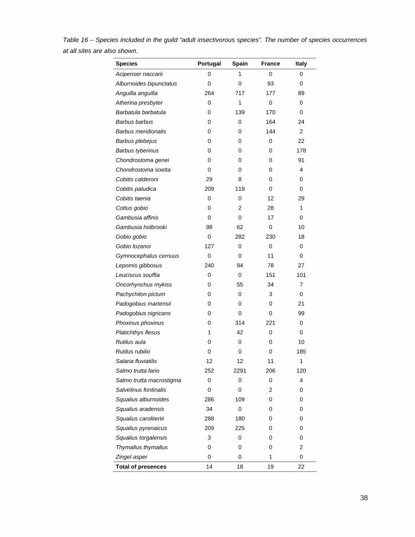
38

Table 16 – Species included in the guild “adult insectivorous species”. The number of species occurrences

at all sites are also shown.

Species Portugal Spain France Italy

Acipenser naccarii 0 1 0 0

Alburnoides bipunctatus 0 0 93 0

Anguilla anguilla 264 717 177 89

Atherina presbyter 0 1 0 0

Barbatula barbatula 0 139 170 0

Barbus barbus 0 0 164 24

Barbus meridionalis 0 0 144 2

Barbus plebejus 0 0 0 22

Barbus tyberinus 0 0 0 178

Chondrostoma genei 0 0 0 91

Chondrostoma soetta 0 0 0 4

Cobitis calderoni 29 8 0 0

Cobitis paludica 209 119 0 0

Cobitis taenia 0 0 12 29

Cottus gobio 0 2 28 1

Gambusia affinis 0 0 17 0

Gambusia holbrooki 98 62 0 10

Gobio gobio 0 282 230 18

Gobio lozanoi 127 0 0 0

Gymnocephalus cernuus 0 0 11 0

Lepomis gibbosus 240 94 78 27

Leuciscus souffia 0 0 151 101

Oncorhynchus mykiss 0 55 34 7

Pachychilon pictum 0 0 3 0

Padogobius martensii 0 0 0 21

Padogobius nigricans 0 0 0 99

Phoxinus phoxinus 0 314 221 0

Platichthys flesus 1 42 0 0

Rutilus aula 0 0 0 10

Rutilus rubilio 0 0 0 185

Salaria fluviatilis 12 12 11 1

Salmo trutta fario 252 2291 206 120

Salmo trutta macrostigma 0 0 0 4

Salvelinus fontinalis 0 0 2 0

Squalius alburnoides 286 109 0 0

Squalius aradensis 34 0 0 0

Squalius carolitertii 288 180 0 0

Squalius pyrenaicus 209 225 0 0

Squalius torgalensis 3 0 0 0

Thymallus thymallus 0 0 0 2

Zingel asper 0 0 1 0

Total of presences 14 18 19 22

39

Predictive Model According to the Akaike’s information Criteria this metric could not be explained by any of the

explanatory environmental variables considered, as only the intercept is included in the final

solution after variable selection (i.e. metric vaues are predicted to be constant along the

environmental gradient) (Table 17). Hence, the scores are simply measuring the deviations from

the mean value of the metrics in calibration sites. Despite this result, this metric was considered

as a good candidate because it had the strongest response to pressures among all tested

metrics.

Table 17 – Coefficients of the poisson regression of the richness of adult insectivorous species against

environmental variables.

Selected Variables

Estimate Std. Error z value Pr(>|z|)

(Intercept) -0.457 0.074 -6.155 7.51E-10

Model diagnosis The resulting model is good according to all four model diagnostic criteria (Fig. 11).

Fig. 11 – Graphical representation of model diagnostic for the richness of adult insectivorous species (From

top left to bottom right: Normal QQ plot; plot of residuals as the function of fitted values; plot of expected

against observed metrics’ values; plot of leverage values against Pearsion residuals).

40

Response to single pressures

The response of the richness of adult insectivorous species to the most relevant single pressure

variables for each pressure type (see section 3.2.2) is represented in figure 12. The response

strength of this metric varied widely according to single pressures. The most evident responses

are to hydrological modifications, water quality index and eutrophication. There are also some

less marked responses to riparian vegetation alterations, water abstraction, channelisation, toxic

substances and impoundment. No response was found to the presence of downstream barriers at

the catchment and segment levels and instream habitat alteration.

Fig. 12 – Boxplots representing score value variations of the richness of adult insectivorous species for

each single pressure intensity (see table 3) of the most relevant pressures (Dashed lines represent the 1st

and 3rd quartils of the calibration sites scores; Barriers_down – presence of a downstream barrier at the

catchment level, Barries_segm_down – presence of a downstream barrier in the river segment,

hydro_modification – hydrological regime modification).

41

Response to combined pressures

In figure 13 the response of the richness of adult insectivorous species to the several combined

pressure variables is expressed by contrasting the differences between scores of the calibration

dataset and scores of the most disturbed sites (pressure index values above the 3rd quartile). This

metric is responsive to all combined pressure variables considered. The metrics is especially

responsive to Global Pressure (PC1), Hydrology (PC1), Water Quality (PC1), Total Pressure

Index and Global Pressure Index (Fig. 10).

Fig. 13 – Boxplots representing score value variations of the richness of adult insectivorous species for the

calibration dataset and for the most disturbed sites.

42

Differences in metrics response among countries As shown in figure 14, this metric is responsive to Global Pressure (PC1) in all four

mediterranean countries. The response is quite strong in Portugal and particularly strong in

France. The scores of the calibration sites are higher for both France and Italy, compared to

Iberian countries, which can be due to the higher richness of insectivorous species found in these

two countries (Table 16).

Fig. 14 – Boxplots representing score value variations of the richness of adult insectivorous species for the

calibration dataset and for the most disturbed sites, according to the Global Pressure (PC1), separately for .

each country.

b) Richness of resident species (Migration guild)

Guild composition This metric comprises 50 species, of which nine are common to the four countries: Alburnus

alburnus, Ameiurus melas, Carassius auratus, Cyprinus carpio, Gambuzia holbrooki, Lampetra

planeri, Lepomis gibbosus, Micropterus salmoides, Salaria fluviatilis (Table 18). The two and very

similar congeneric species of Gobio (G. gobio and G. lozanoi) are also common to the four

countries. The most represented and widespread taxa within this metrics are G. gobio / lozanoi

and L. gibbosus.

43

Table 18 – Species included in the guild “richness of resident species”. The number of species occurrences

at all sites are also shown.


Achondrostoma arcasii 82 205 0 0

Achondrostoma occidentale 1 0 0 0

Achondrostoma oligolepis 153 0 0 0


Alburnus albidus 0 0 0 2

Alburnus alburnus 1 19 116 90

Ameiurus melas 1 17 17 18

Anaecypris hispanica 5 3 0 0

Atherina boyeri 18 1 0 2


Carassius auratus 53 33 19 69

Carassius carassius 0 0 33 2


Cobitis paludica 209 119 0 0

Cobitis taenia 0 0 12 29


Cyprinus carpio 55 44 43 67

Gambusia holbrooki 98 62 17 10

Gasterosteus aculeatus 0 0 8 17

Gasterosteus gymnurus 10 72 0 0



Gymnocephalus cernuus 0 0 11 0

Iberochondrostoma almacai 18 0 0 0

Iberochondrostoma lusitanicum 28 0 0 0

Lampetra planeri 15 2 3 8

Lepomis gibbosus 240 94 78 27

Leuciscus leuciscus 0 0 95 0


Micropterus salmoides 87 40 4 11

Pachychilon pictum 0 0 3 0



Perca fluviatilis 0 0 48 10


Pseudorasbora parva 0 0 14 37

Rhodeus amarus 0 0 9 1

Rutilus aula 0 0 0 10


Salaria fluviatilis 12 12 11 1

44

(Cont.)


Scardinius erythrophthalmus 0 0 15 15

Silurus glanis 0 0 6 1






Tinca tinca 0 5 46 30



Predictive Model

As shown in tables 19 and 20 the predictive model using the richness of resident species as

response variable, two explanatory variables were selected in the final model solution: altitude,

with a negative effect, and siliceous bedrock, with a positive effect on the metric.

Table 19 – Coefficients of the poisson regression of the richness of resident species against environmental

variables.


(Intercept) -1.250 0.296 -4.227 0.000

Altitude -0.000 0.000 -1.612 0.107

Geological typology - Siliceous 0.712 0.293 2.430 0.015

Table 20 – Sequential analysis of deviance for the model using the richness of resident species as

response variable (the reductions in the residual deviance as each term of the formula is added in turn are

given)

Df Deviance Resid. Df Resid. Dev

NULL NA NA 79.000 45.746

Altitude 1.000 2.589 78.000 43.156


45

Model diagnosis The resulting predictive model is good according to all four model diagnostic criteria (Fig. 15),

though there are some potential leverage points.

Fig. 15 – Graphical representation of model diagnostic for the richness of resident species (From top left to

bottom right: Normal QQ plot; plot of residuals as the function of fitted values; plot of expected against

observed metrics’ values; plot of leverage values against Pearson residuals).


The response of the richness of resident species to the most relevant single pressure variables

for each pressure type (see section 3.2.2) is represented in figure 16. This metric responds

weakly to some single pressure variables, such as water abstraction, riparian vegetation

alteration and toxic substances. No evident responses were found for the remaining pressures.

46

Fig. 16 – Boxplots representing score value variations of the richness of resident species for each single

pressure intensity (see table 3) of the most relevant pressures (Dashed lines represent the 1st and 3rd

quartils of the calibration sites scores; Barriers_down – presence of a downstream barrier at the catchment

level, Barries_segm_down – presence of a downstream barrier in the river segment, hydro_modification –

hydrological regime modification).

Response to combined pressures In figure 17 the response of the richness of resident species to the several combined pressure

variables is expressed by contrasting the differences between scores of the calibration dataset

and scores of the most disturbed sites (pressure index values above the 3rd quartile). This metric

is only weakly responsive to most the combined pressure variables considered. The strongest

responses of this metric were to Morphology (PC1), Water Quality (PC1) and Water Alteration

Index (Fig. 17).

47

Fig. 17 – Boxplots representing score value variations of the richness of resident species for the calibration

dataset and for the most disturbed sites.

Differences in metrics response among countries As shown in figure 18, this metric is responsive in France and Spain, but not in Portugal. This can

be due to the strong representation of species such as Phoxinus phoxinus (the most frequent

species of this guild; see Table 18) and Barbatula barbatula in France and Spain, which are

absent from Portugal, and also possibly to the exclusive presence of the abundant native species,

Achondrostoma oligolepis, in Portugal. In Italy there is no highly disturbed sites according to the

Global Index (PC1) and therefore no conclusions can be draw about metrics response, though

the scores of the calibration dataset are too low in this country.

48


dataset and for the most disturbed sites, according to the Global Pressure (PC1), separately for . each

country.

c) Richness of potamodromous species (Migration guild)

Guild composition This metric comprises 34 species, of which only two are common to the four countries: Liza

ramada and Salmo trutta fario (Table 21). The most represented taxa within this metrics are S.

trutta fario, Barbus bocagei and Pseudochondrostoma duriense, the later two only occurring in

the Iberian countries. It should be noted that S. trutta fario, although being considered a

potamodromous species, performs much shorter range movements in southern Europe countries.

49

Table 21 – Species included in the guild “richness of potamodromous species”. The number of species

occurrences at all sites are also shown.


Abramis brama 0 0 21 0


Barbus bocagei 383 141 0 0

Barbus comizo 78 27 0 0

Barbus graellsii 0 90 0 3

Barbus guiraonis 0 68 0 0

Barbus haasi 0 26 0 0


Barbus microcephalus 44 20 0 0


Barbus sclateri 44 84 0 0


Chondrostoma arrigonis 0 8 0 0


Chondrostoma miegii 0 112 0 0

Chondrostoma nasus 0 0 44 0


Chondrostoma toxostoma 0 0 75 0

Chondrostoma turiense 0 6 0 0

Esox lucius 0 18 30 5

Iberochondrostoma lemmingii 46 35 0 0

Leuciscus cephalus 0 1 266 190

Leuciscus lucumonis 0 0 0 97

Liza aurata 0 1 1 0

Liza ramada 19 1 5 1


Pseudochondrostoma duriense 202 451 0 0

Pseudochondrostoma polylepis 216 119 0 0

Pseudochondrostoma willkommii 36 26 0 0

Rutilus rutilus 0 1 145 1



Sander lucioperca 0 2 8 8



50

Predictive Model As shown in tables 22 and 23 the predictive model using the richness of potamodromous species

as response variable, the same two explanatory variables as those selected for the richness of

resident species, were selected in the final model solution: altitude, with a positive effect, and

siliceous bedrock, with a negative effect on the metric.

Table 22 – Coefficients of the poisson regression of the richness of potamodromous species against



(Intercept) -0.677 0.198 -3.424 0.001

Altitude 0.001 0.000 2.722 0.006

Geological typology - Siliceous -0.390 0.193 -2.023 0.043

Table 23 – Sequential analysis of deviance for the model using the richness of potamodromous species as

response variable (the reductions in the residual deviance as each term of the formula is added in turn are

given)


NULL NA NA 79.000 35.800

Altitude 1.000 6.693 78.000 29.107


Model diagnosis The resulting predictive model is good (residual normality and structure) or acceptable (expected

versus observed and leverage versus against residuals) according to the four model diagnostic

criteria (Fig. 19).

51

Fig. 19 – Graphical representation of model diagnostic for the richness of potamodromous species (from

top left to bottom right: Normal QQ plot; plot of residuals as the function of fitted values; plot of expected

against observed metrics’ values; plot of leverage values against Pearson residuals).

Response to single pressures The response of the richness of potamodromous species to the most relevant single pressure

variables for each pressure type (see section 3.2.2) is represented in figure 20. This metric

responds more evidently to three single pressure variables: channelisation, riparian vegetation

alteration and toxic substances. There are also some less marked responses to water

abstraction, instream habitat alteration and Water Quality Index. No evident responses were

found for the remaining pressures.

52

Fig. 20 – Boxplots representing score value variations of the richness of potamodromous species for each

single pressure intensity (see table 3) of the most relevant pressures (Dashed lines represent the 1st and 3rd

quartils of the calibration sites scores; Barriers_down – presence of a downstream barrier at the catchment

level, Barries_segm_down – presence of a downstream barrier in the river segment, hydro_modification –

hydrological regime modification).

Response to combined pressures In figure 21 the response of the richness of potamodromous species to the several combined



metric is responsive to all combined pressure variables considered, with differing strengths. The

metrics is especially responsive to Morphology (PC1), Habitat Index and Total Pressure Index

(Fig. 21). For the remaining combined pressure variables there is a wide overlap of score

distributions between calibration and highly disturbed sites.

53

Fig. 21 – Boxplots representing score value variations of the richness of potamodromous species for the


Differences in metrics response among countries

As shown in figure 22, this metric is clearly responsive in France, but for Portugal and Spain there

is a wide overlap of score distributions between calibration and highly disturbed sites. In Italy

there is no highly disturbed sites according to the Global Index (PC1) and therefore no

conclusions can be draw about metrics response, though the scores of the calibration dataset are

comparable to the other country.

54


dataset and for the most disturbed sites, according to the Global Pressure (PC1), separately for . each

country.

d) Richness of rheophilic spawning species (spawning habitat guild)

Guild composition

This metric comprises 54 taxa, of which only three are common to the four countries: Lampetra

planeri, Gobio gobio/lozanoi and Salmo trutta fario (Table 24). The most represented taxa within

this metrics are S. trutta fario, Gobio gobio/lozanoi, Barbus bocagei and Pseudochondrostoma

duriense, the later two only occurring in the Iberian countries.

Table 24 – Species included in the guild “richness of rheophilic spawning species”. The number of species



Achondrostoma arcasii 82 205 0 0

Achondrostoma occidentale 1 0 0 0

Achondrostoma oligolepis 153 0 0 0



Alosa fallax 1 0 0 0

55

(Cont.)

Anaecypris hispanica 5 3 0 0





















Dicentrarchus labrax 0 0 1 0



Hypophthalmichthys molitrix 0 0 1 0

Iberochondrostoma almacai 18 0 0 0

Iberochondrostoma lemmingii 46 35 0 0

Iberochondrostoma lusitanicum 28 0 0 0

Lampetra fluviatilis 10 0 0 0









Petromyzon marinus 13 50 0 0





Salmo salar 0 145 0 0

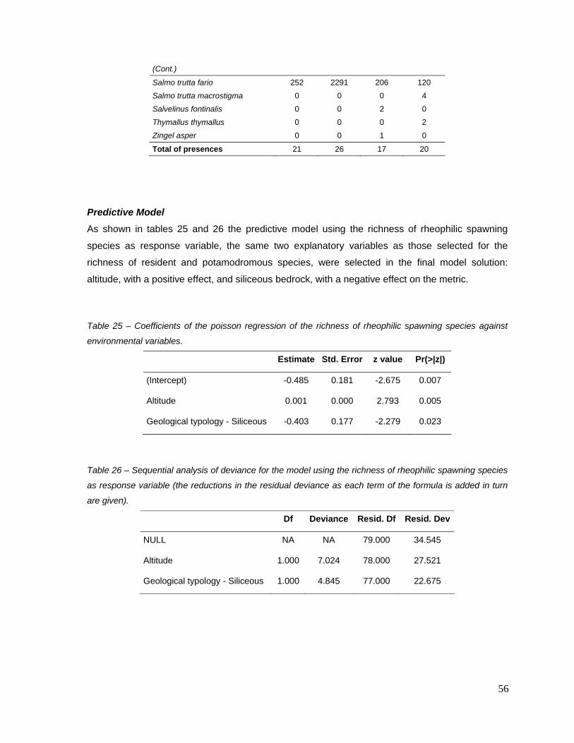
56

(Cont.)







Predictive Model As shown in tables 25 and 26 the predictive model using the richness of rheophilic spawning

species as response variable, the same two explanatory variables as those selected for the

richness of resident and potamodromous species, were selected in the final model solution:

altitude, with a positive effect, and siliceous bedrock, with a negative effect on the metric.

Table 25 – Coefficients of the poisson regression of the richness of rheophilic spawning species against



(Intercept) -0.485 0.181 -2.675 0.007

Altitude 0.001 0.000 2.793 0.005

Geological typology - Siliceous -0.403 0.177 -2.279 0.023

Table 26 – Sequential analysis of deviance for the model using the richness of rheophilic spawning species

as response variable (the reductions in the residual deviance as each term of the formula is added in turn

are given).


NULL NA NA 79.000 34.545

Altitude 1.000 7.024 78.000 27.521


57

Model diagnosis The resulting predictive model is good according to the model diagnostic criteria, though there are

some potential leverage points (Fig. 23).

Fig. 23 – Graphical representation of model diagnostic for the richness of rheophilic spawning species

(From top left to bottom right: Normal QQ plot; plot of residuals as the function of fitted values; plot of

expected against observed metrics’ values; plot of leverage values against Pearson residuals).

Response to single pressures The response of the richness of rheophilic spawning species to the most relevant single pressure


responds more evidently to two single pressure variables: channelization and toxic substances.

There are also some less marked responses to water abstraction and riparian vegetation

alteration. No evident responses were found for the remaining pressures.

58

Fig. 24 – Boxplots representing score value variations of the richness of rheophilic spawning species for

each single pressure intensity (see table 3) of the most relevant pressures (dashed lines represent the 1st




Response to combined pressures In figure 25 the response of the richness of rheophilic spawning species to the several combined



metric is only weakly responsive to most combined pressure variables considered. Stronger

trends are found in the responses to Water Quality (PC1), Habitat Index and Global Pressure

Index (Fig. 25). For the remaining combined pressure variables there is a wide overlap of score


59

Fig. 25 – Boxplots representing score value variations of the richness of rheophilic spawning species for the


Differences in metrics response among countries

As shown in figure 26, this metric is clearly responsive in France, but for Portugal and Spain there

is a wide overlap of score distributions between calibration and highly disturbed sites. In Italy

there is no highly disturbed sites according to the Global Index (PC1) and therefore no

conclusions can be draw about metrics response, though the scores of the calibration dataset are

comparable to the other country.

60

Fig. 26 – Boxplots representing score value variations of the richness of rheophilic spawning species for the


each country.

e) Richness of lithophilic spawning species (spawning substrate guild)

Guild composition This metric comprises 46 taxa, of which only three are common to the four countries: Ameiurus

melas, Lampetra planeri and Salmo trutta fario (Table 27). The most represented taxa within this

metrics are S. trutta fario, Phoxinus phoxinus (occurring only in Spain and France), Barbus

bocagei and Pseudochondrostoma duriense (both occurring only in Spain and Portugal).

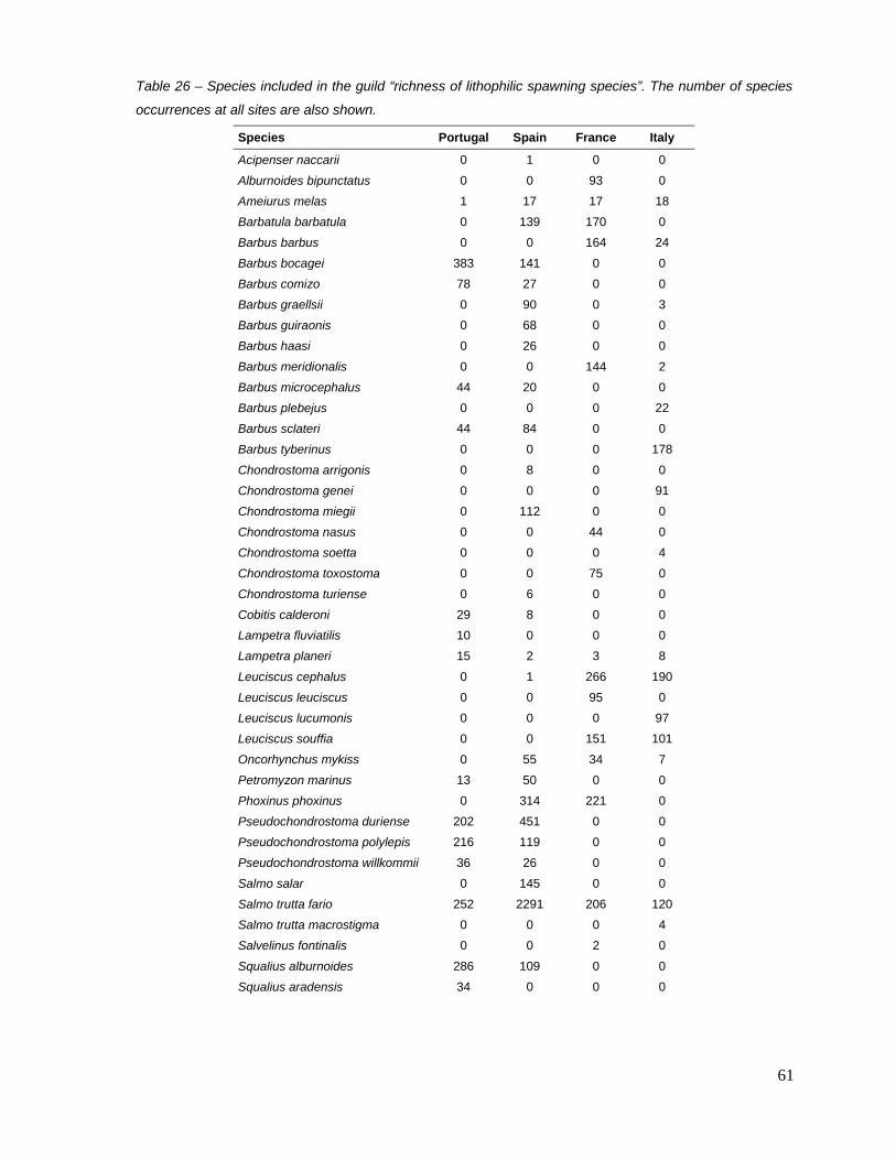
61

Table 26 – Species included in the guild “richness of lithophilic spawning species”. The number of species





Ameiurus melas 1 17 17 18





















Lampetra fluviatilis 10 0 0 0







Petromyzon marinus 13 50 0 0





Salmo salar 0 145 0 0






62

(Cont.)







Predictive Model As shown in tables 28 and 29 the predictive model using the richness of lithophilic spawning

species as response variable, two explanatory variables were selected in the final model solution:

the first latent geomorphological variable, with a negative effect, and the thermal amplitude, with a

positive effect on the metric.

Table 28 – Coefficients of the poisson regression of the richness of lithophilic spawning species against



(Intercept) -1.740 0.600 -2.897 0.004

Geomorphology PC1 -0.310 0.139 -2.227 0.026

Thermal amplitude 0.082 0.036 2.281 0.023

Table 29 – Sequential analysis of deviance for the model using the richness of lithophilic spawning species

as response variable (the reductions in the residual deviance as each term of the formula is added in turn

are given).


NULL NA NA 79.000 27.079

Geomorphology PC1 1.000 2.267 78.000 24.812

Thermal amplitude 1.000 5.270 77.000 19.541

63

Model diagnosis The resulting predictive model is good (residual normality and structure) or acceptable (expected

versus observed and leverage versus against residuals) according to the four model diagnostic

criteria (Fig. 27).

Fig. 27 – Graphical representation of model diagnostic for the richness of lithophilic spawning species

(From top left to bottom right: Normal QQ plot; plot of residuals as the function of fitted values; plot of

expected against observed metrics’ values; plot of leverage values against Pearsion residuals).


The response of the richness of lithophilic spawning species to the most relevant single pressure


responds evidently to toxic substances, with no evident responses found for the remaining

pressures.

64

Fig. 28 – Boxplots representing score value variations of the richness of lithophilic spawning species for

each single pressure intensity (see table 3) of the most relevant pressures (Dashed lines represent the 1st




Response to combined pressures

In figure 29 the response of the richness of lithophilic spawning species to the several combined



metric is only weakly responsive to most combined pressure variables considered. The strongest

responses were found for Water Quality (PC1) and, to a lesser degree, for Global Pressure Index

65

(Fig. 26). For the remaining combined pressure variables there is a wide overlap of score


Fig. 29 – Boxplots representing score value variations of the richness of lithophilic spawning species for the


Differences in metrics response among countries As shown in figure 30, this metric is clearly responsive in France, although the scores of the

calibration dataset are well below the expected value (0.5). For Spain the metric is also

responsive, although there is a wide overlap of score distributions between calibration and highly

disturbed sites. For Portugal no evident response was found. As mentioned for the other

candidate metrics, in Italy there is no highly disturbed sites according to the Global Index (PC1)

and therefore no conclusions can be draw about metrics response. The scores of the calibration

dataset are very low but are comparable to those found for the French sites.

66

Fig. 30 – Boxplots representing score value variations of the richness of lithophilic spawning species for the


each country.

3.5.5.4 Summary of metrics’ response to pressure

Overall, among the single pressure variables to which metrics’ response was graphically explored

in this report, only few had an evident effect on some metrics (Table 30). The single pressures to

which there were more frequent evident responses among the final candidate metrics were the

presence of toxic substances (4 metric responses), channelisation and riparian vegetation

alteration (both with two responses). Hydrological modification, water abstraction, water quality

index and eutrophication were shown to have an evident effect at least for one metric.

67

Table 30 – Stronger responses of each metric to the most relevant single pressure variables.

Metric

Richness of adult

insectivorous species

Richness of

resident species

Richness of potamodromous

species

Richness of

rheophilic spawning species

Richness of lithophilic spawning species

Presence of barriers downstream at the catchment

Presence of barriers downstream at the river segment

Impoundment

Hydrological modification

Water abstraction

Channelisation

Riparian vegetation alteration

Instream habitat alteration

Water Quality Index

Eutrofication

Toxic substances

In comparison to responses to single pressure variables, more evident candidate metrics

reponses to combined pressure variables were found (Table 31). The combined pressures to

which there were more frequent evident responses among the final candidate metrics were the

PC1 Water Quality (4 metric responses), PC1 Morphology, Habitat Alteration index and Global

Pressure Index (all with three responses). The metric “richness of adult insectivorous species”

responded quite evidently to all the combined pressure variables considered.

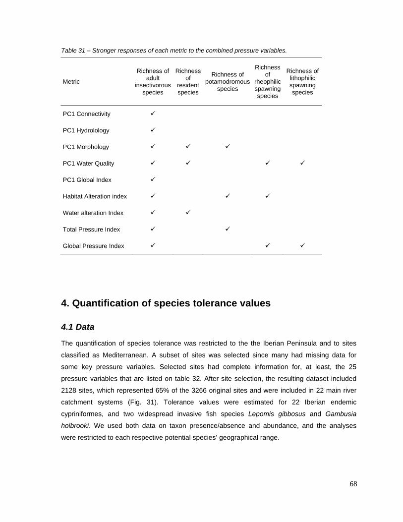
68

Table 31 – Stronger responses of each metric to the combined pressure variables.

Metric

Richness of adult

insectivorous species

Richness of

resident species

Richness of potamodromous

species

Richness of

rheophilic spawning species

Richness of lithophilic spawning species

PC1 Connectivity

PC1 Hydrolology

PC1 Morphology

PC1 Water Quality

PC1 Global Index

Habitat Alteration index

Water alteration Index

Total Pressure Index

Global Pressure Index

4. Quantification of species tolerance values

4.1 Data

The quantification of species tolerance was restricted to the the Iberian Peninsula and to sites

classified as Mediterranean. A subset of sites was selected since many had missing data for

some key pressure variables. Selected sites had complete information for, at least, the 25

pressure variables that are listed on table 32. After site selection, the resulting dataset included

2128 sites, which represented 65% of the 3266 original sites and were included in 22 main river

catchment systems (Fig. 31). Tolerance values were estimated for 22 Iberian endemic

cypriniformes, and two widespread invasive fish species Lepomis gibbosus and Gambusia

holbrooki. We used both data on taxon presence/absence and abundance, and the analyses

were restricted to each respective potential species’ geographical range.

69

Table 32 – Species used as taxa-based metrics, total relative abundance (number per ha x 104), number of occurrence sites (total and calibration) and potential area of distribution.

Species Total abundance

Number of sites

Number of calibration sites

Distribution (river basins)

Achondrostoma arcasii 19.30 155 25 • Cantabrica, Catalana, Douro, Ebro, Galaica, Guadiana, Minho, Tejo, Valenciana.

Achondrostoma oligolepis 15.98 132 2 • Ave, Cavado, Douro, Lima, Lis, Mondego, Oeste, Tejo, Vouga

Anaecypris hispanica 0.03 5 2 • Guadiana Barbus bocagei 39.12 408 27 • Ave, Cavado, Douro, Galaica,

Lima, Lis, Minho, Mondego, Oeste, Sado, Tejo, Vouga

Barbus comizo 9.25 91 1 • Guadiana, Tejo Barbus graellsii 16.79 85 3 • Cantabrica, Catalana, Ebro Barbus haasi 0.25 14 2 • Catalana, Ebro, Valenciana Barbus microcephalus 4.56 51 2 • Guadiana Barbus sclateri 15.34 78 22 • Algarve, Guadalquivir, Guadiana,

Mira, Segura, Sur Chondrostoma miegii 5.75 66 3 • Ebro Cobitis calderoni 0.90 39 1 • Ave, Cavado, Douro, Ebro, Lima,

Minho, Tejo, Cobitis paludica 9.07 245 23 • Algarve, Cantabrica, Catalana,

Douro, Ebro, Galaica, Guadalquivir, Guadiana, Lis, Mira, Mondego, Oeste, Sado, Sur, Tejo, Valenciana, Vouga

Iberochondrostoma almacai 0.53 18 7 • Algarve, Mira Iberochondrostoma lemmingii 1.83 54 4 • Algarve, Douro, Guadalquivir,

Guadiana, Sado, Tejo Iberochondrostoma lusitanicum 2.40 28 0 • Oeste, Sado, Tejo Pseudochondrostoma duriense 54.53 433 87 • Ave, Cavado, Douro, Galaica,

Lima, Minho Pseudochondrostoma polylepis 23.79 245 20 • Algarve, Lis, Mondego, Oeste,

Sado, Segura, Tejo, Valenciana, Vouga

Pseudochondrostoma willkommii 3.43 48 2 • Guadalquivir, Guadiana, Sur Squalius alburnoides 33.85 308 14 • Douro, Guadalquivir, Guadiana, Lis,

Mondego, Sado, Tejo, Vouga Squalius aradensis 5.94 34 15 • Algarve Squalius carolitertii 27.74 336 43 • Ave, Cavado, Douro, Ebro, Galaica,

Lima, Minho, Mondego, Vouga Squalius pyrenaicus 39.19 272 35 • Ebro, Guadalquivir, Guadiana,

Oeste, Sado, Segura, Sur, Tejo, Valenciana

Gambusia holbrooki 11.18 112 1 • Algarve, Ave, Catalana, Cavado, Douro, Ebro, Guadalquivir, Guadiana, Lima, Lis, Mira, Mondego, Oeste, Sado, Segura, Tejo, Valenciana, Vouga"

Lepomis gibbosus 21.38 263 3 • Algarve, Catalana, Douro, Ebro, Guadalquivir, Guadiana, Lis, Minho, Mira, Mondego, Oeste, Sado, Segura, Sur, Tejo, Valenciana, Vouga"

70

Fig. 31 – Selected sites and respective catchment names

4.2 Statistical analyses

As a first approach to assess the indicator value of species we estimated species tolerance based

on estimations of optimal conditions and niche breath with respect to each pressure-type

combination and global pressures. Two simple alternative approaches were used: the quadratic

logistic regression and the weighted averaging approaches (e.g. ter Braak & Looman 1986;

Jongman et al. 1995).

The quadratic or Gaussian logistic regression (QLR) estimates a species response curve from

presence-absence data using a second-order polynomial in the environmental variable as linear

predictor. Theoretically this curve assumes a Gaussian species response curve, i.e., a symmetric

unimodal curve describing species probability of occurrence along the environmental gradient, for

which it is possible to estimate optimum condition (or niche position) and tolerance (or niche

breath) values. The quadratic logistic function is expressed by:

2210)(1

)(log xbxbbxp

xp++=⎥

⎦

⎤⎢⎣

⎡−

71

where p(x) is the probability of a species to occur as a function of x. The optimum and tolerance

can be obtained as follows:

Optimum ( )221 bbu −=

Tolerance )2(1 2bt −=

In this study we considered the upper tolerance (u + t) value (sensu ecological literature) as an

estimator of species tolerance (sensu biotic integrity assessment literature) to pressures.

The method of weighted averaging (WA) is a simpler alternative to regression methods that

circumvents the problem of fitting a particular response curve. This method has been long used in

ecology and recently, as in the present study, it was used to quantify species tolerance to

pressures in the context of biotic integrity assessments of rivers (Whittier et al. 2007; Welsh &

Hodgson in press). The species optimum is simply obtained by taking the average of the values

of the environmental variables (xi) weighted by species abundance (yik), over those sites where

the species is present (Jongman et al. 1995). Species tolerance is given by one standard

deviation of the optimum. Optimum and tolerance are expressed as follows:

Optimum

∑

∑

=

== n

iik

n

iiik

y

xyu

1

1

Tolerance ( )

∑

∑

=

=

−= n

iik

n

iiik

y

uxyt

1

1

2

Here we used the bootstrap approach recommended by Whittier et al. (2007) in order to obtain

more robust estimates of upper tolerance (u + t) values, particularly of those species collected in

few sites.

The main disadvantages of the WA method is that it disregards absences and can give

misleading results if the sampling is too uneven distributed along the environmental gradient (ter

72

Braak & Looman, 1986). On the other hand the QLR has the main disadvantage of requiring an

unimodal response for optima and tolerance to be estimated. Nevertheless, the two methods

gives similar results in case of species with low probability of occurrence and/or narrow tolerance

(ter Braak & Looman, 1986).

For comparison purposes, the upper tolerance values estimated with both approaches were

rescaled in order to vary between 1 and 10 using the expression: 10*(species upper tolerance –

minimum score) / range of values.

4.3 Estimated tolerances

Although the two approaches to species upper tolerance estimation produced distinct results,

they evidenced similar general trends (Tables 33 and 34; figures 32 to 34), namely: (1) according

to both methods, large cyprinids are more often tolerant to a greater number of pressure

combined variables than small cyprinids (Tables 33 and 34); (2) only in very few cases there are

high discrepancies between the two methods (e.g. P. duriense; Fig. 33 to 34); (3) many species

were consistently ranked according to upper tolerance values (e.g. S. aradensis, I. almacai and A.

hispanica as globally intolerant species and G. holbrookii and B. bocagei as globally tolerant

species; Fig. 33 to 34).

Nevertheless, for some species the estimated upper tolerances differed greatly between

methods. For example, using the QLR approach the estimated upper tolerance of P. duriensis

and A. arcasii was much higher, while that of I. lusitanicum, P. polylepis, C. miegii, B. graellsii was

much lower.

An important difference between the results of the two approaches is that the QLR estimates

species’ tolerances that may go beyond the conditions experienced by species (S. aradensis and

P. duriense; Fig. 34). This is due to the fact that this method is based on the estimation of a

theoretical response curve to pressures. In opposition, the WA method always predicts tolerances

that are included within the range of conditions experienced by species (Fig. 34).

73

Table 33 – Rescaled upper species’ tolerance values according to the quadratic logistic regression approach (empty cells correspond to non-unimodal relationships between species presence and pressure).

Species Connect. Hydrol. Morphol. Water quality Global

Small cyprinids

Achondrostoma arcasii 2.86 1.14 4.16 6.47

Achondrostoma oligolepis 10.00 3.43 3.28 4.86

Anaecypris hispanica 0.01 0.32 1.66

Iberochondrostoma almacai 0.00 4.96 1.85

Iberochondrostoma lemmingii 0.80 1.03 1.82 4.15 3.00 Iberochondrostoma lusitanicum 0.70 3.87 5.68 5.04

Squalius alburnoides 1.84 2.04 0.69 4.54 5.21

Squalius aradensis 0.03 0.06 0.37 0.00

Squalius carolitertii 4.65 1.87 2.56 3.56 3.37

Squalius pyrenaicus 1.53 4.34 1.30

Large cyprinids

Barbus bocagei 1.99 2.20 4.44 4.58 6.29

Barbus comizo 10.00 1.19 1.60 5.01 4.08

Barbus graellsii 0.19 0.46 4.86 3.28 5.83

Barbus haasi 0.80 2.76 10.00 0.00 6.43

Barbus microcephalus 0.90 3.27 0.00 10.00 3.94

Barbus sclateri 2.74 0.71 1.00 2.15 0.86

Chondrostoma miegii 0.00 0.53 5.21 2.86 5.71 Pseudochondrostoma duriense 3.72 1.81 4.60 10.00 Pseudochondrostoma polylepis 3.17 2.14 3.95 8.18 Pseudochondrostoma willkommii 0.60 1.48 1.73 4.47 3.77

Cobitids

Cobitis calderoni 1.98 1.79 4.03 3.22 4.63

Cobitis paludica 3.75 5.24 5.88

Exotic

Lepomis gibbosus 2.48 2.70 4.61 5.71 6.53

Gambusia holbrooki 6.20 2.91 6.72 6.99 8.86

74

Table 34 – Rescaled bootstrap estimates of upper species’ tolerance values according to the weighted averaging method.

Species Connect. Hydrol. Morphol. Water quality Global

Small cyprinids

Achondrostoma arcasii 4.57 4.73 4.73 2.74 3.38

Achondrostoma oligolepis 3.45 4.85 5.70 4.88 6.00

Anaecypris hispanica 0.17 0.94 0.15 4.49 0.21

Iberochondrostoma almacai 0.00 0.00 0.00 3.53 0.09

Iberochondrostoma lemmingii 1.74 3.04 1.62 7.80 3.99

Iberochondrostoma lusitanicum 1.30 1.96 4.90 10.00 7.46

Squalius alburnoides 4.26 8.81 2.98 6.55 5.46

Squalius aradensis 0.07 0.63 0.45 3.03 0.17

Squalius carolitertii 7.36 4.46 2.09 3.05 0.00

Squalius pyrenaicus 3.94 5.37 2.35 4.52 1.97

Large cyprinids

Barbus bocagei 6.06 9.28 4.53 7.04 6.90

Barbus comizo 5.41 8.59 1.04 7.43 3.52

Barbus graellsii 0.36 1.01 10.00 2.88 10.00

Barbus haasi 2.11 3.09 8.52 0.00 7.89

Barbus microcephalus 2.86 10.00 1.22 4.88 3.61

Barbus sclateri 4.23 4.34 2.52 1.27 1.08

Chondrostoma miegii 1.04 2.16 9.78 2.70 9.79

Pseudochondrostoma duriense 10.00 5.58 3.05 4.16 0.99

Pseudochondrostoma polylepis 5.94 9.48 3.66 5.06 4.59

Pseudochondrostoma willkommii 4.20 7.05 2.69 4.28 3.48

Cobitids

Cobitis calderoni 5.99 8.65 4.14 2.33 3.74

Cobitis paludica 2.60 4.15 4.58 6.86 6.19

Exotic

Lepomis gibbosus 4.10 7.87 3.57 6.54 4.97

Gambusia holbrooki 2.92 6.88 4.36 8.85 9.07

75

Fig. 32 – Species fitted response curves to global pressure according to the quadratic logistic regression approach. Upper tolerance values (vertical solid line) and the available range of conditions at the species potential area of distribution (two vertical dashed lines representing the 1st and the 99th percentiles) are also represented.

76

Fig. 33 – Scatter plot of species relative abundance along the global pressure gradient. Upper tolerance values estimated with the weighted averaging approach (vertical solid line) and the available range of conditions at the species potential area of distribution (two vertical dashed lines representing the 1st and the 99th percentiles) are also represented.

77

Fig. 34 – Estimates of species tolerance to global pressure according to the quadratic logistic regression approach (a) and (b) weighted averaging approach. Species are ordered by increasing upper tolerance. The available range of conditions at the potential distribution range of each species is also represented.

a)

Exotic

Small cyprinids

Large cyprinidsToleranceRange of conditions available (1st and 99th percentiles)

-10.00

-5.00

0.00

5.00

10.00

15.00

Squ

aliu

s ar

aden

sis

Bar

bus

scla

teri

Squ

aliu

s py

rena

icus

Ana

ecyp

ris h

ispa

nica

Iber

ocho

ndro

stom

a al

mac

ai

Iber

ocho

ndro

stom

a le

mm

ingi

i

Squa

lius

caro

liter

tii

Pse

udoc

hond

rost

oma

willk

omm

ii

Bar

bus

mic

roce

phal

us

Bar

bus

com

izo

Cob

itis

cald

eron

i

Ach

ondr

osto

ma

olig

olep

is

Iber

ocho

ndro

stom

a lu

sita

nicu

m

Squa

lius

albu

rnoi

des

Cho

ndro

stom

a m

iegi

i

Barb

us g

rael

lsii

Cob

itis

palu

dica

Bar

bus

boca

gei

Bar

bus

haas

i

Ach

ondr

osto

ma

arca

sii

Lepo

mis

gib

bosu

s

Pse

udoc

hond

rost

oma

poly

lepi

s

Gam

busi

a ho

lbro

oki

Pse

udoc

hond

rost

oma

durie

nseCom

bine

d gl

obal

pre

ssur

e (P

C1

scor

es)

ExoticExotic

Small cyprinids

Large cyprinids

Small cyprinids

Large cyprinids

Small cyprinids

Large cyprinidsToleranceRange of conditions available (1st and 99th percentiles)

-10.00

-5.00

0.00

5.00

10.00

15.00

Squ

aliu

s ar

aden

sis

Bar

bus

scla

teri

Squ

aliu

s py

rena

icus

Ana

ecyp

ris h

ispa

nica

Iber

ocho

ndro

stom

a al

mac

ai

Iber

ocho

ndro

stom

a le

mm

ingi

i

Squa

lius

caro

liter

tii

Pse

udoc

hond

rost

oma

willk

omm

ii

Bar

bus

mic

roce

phal

us

Bar

bus

com

izo

Cob

itis

cald

eron

i

Ach

ondr

osto

ma

olig

olep

is

Iber

ocho

ndro

stom

a lu

sita

nicu

m

Squa

lius

albu

rnoi

des

Cho

ndro

stom

a m

iegi

i

Barb

us g

rael

lsii

Cob

itis

palu

dica

Bar

bus

boca

gei

Bar

bus

haas

i

Ach

ondr

osto

ma

arca

sii

Lepo

mis

gib

bosu

s

Pse

udoc

hond

rost

oma

poly

lepi

s

Gam

busi

a ho

lbro

oki

Pse

udoc

hond

rost

oma

durie

nseCom

bine

d gl

obal

pre

ssur

e (P

C1

scor

es)

ToleranceRange of conditions available (1st and 99th percentiles)


-10.00

-5.00

0.00

5.00

10.00

15.00

Squ

aliu

s ar

aden

sis

Bar

bus

scla

teri

Squ

aliu

s py

rena

icus

Ana

ecyp

ris h

ispa

nica

Iber

ocho

ndro

stom

a al

mac

ai

Iber

ocho

ndro

stom

a le

mm

ingi

i

Squa

lius

caro

liter

tii

Pse

udoc

hond

rost

oma

willk

omm

ii

Bar

bus

mic

roce

phal

us

Bar

bus

com

izo

Cob

itis

cald

eron

i

Ach

ondr

osto

ma

olig

olep

is

Iber

ocho

ndro

stom

a lu

sita

nicu

m

Squa

lius

albu

rnoi

des

Cho

ndro

stom

a m

iegi

i

Barb

us g

rael

lsii

Cob

itis

palu

dica

Bar

bus

boca

gei

Bar

bus

haas

i

Ach

ondr

osto

ma

arca

sii

Lepo

mis

gib

bosu

s

Pse

udoc

hond

rost

oma

poly

lepi

s

Gam

busi

a ho

lbro

oki

Pse

udoc

hond

rost

oma

durie

nseCom

bine

d gl

obal

pre

ssur

e (P

C1

scor

es)

b)

-8.00

-6.00

-4.00

-2.00

0.00

2.00

4.00

6.00

8.00

10.00

Squ

aliu

s ca

rolit

ertii

Iber

ocho

ndro

stom

a al

mac

ai

Squ

aliu

s ar

aden

sis

Ana

ecyp

ris h

ispa

nica

Pse

udoc

hond

rost

oma

durie

nse

Bar

bus

scla

teri

Squ

aliu

s py

rena

icus

Bar

bus

com

izo

Ach

ondr

osto

ma

arca

sii

Pse

udoc

hond

rost

oma

willk

omm

ii

Bar

bus

mic

roce

phal

us

Cob

itis

cald

eron

i

Iber

ocho

ndro

stom

a le

mm

ingi

i

Pse

udoc

hond

rost

oma

poly

lepi

s

Lepo

mis

gib

bosu

s

Squ

aliu

s al

burn

oide

s

Cob

itis

palu

dica

Ach

ondr

osto

ma

olig

olep

is

Bar

bus

boca

gei

Bar

bus

haas

i

Iber

ocho

ndro

stom

a lu

sita

nicu

m

Gam

busi

a ho

lbro

oki

Cho

ndro

stom

a m

iegi

i

Bar

bus

grae

llsii


Com

bine

d gl

obal

pre

ssur

e (P

C1

scor

es)

-8.00

-6.00

-4.00

-2.00

0.00

2.00

4.00

6.00

8.00

10.00

Squ

aliu

s ca

rolit

ertii

Iber

ocho

ndro

stom

a al

mac

ai

Squ

aliu

s ar

aden

sis

Ana

ecyp

ris h

ispa

nica

Pse

udoc

hond

rost

oma

durie

nse

Bar

bus

scla

teri

Squ

aliu

s py

rena

icus

Bar

bus

com

izo

Ach

ondr

osto

ma

arca

sii

Pse

udoc

hond

rost

oma

willk

omm

ii

Bar

bus

mic

roce

phal

us

Cob

itis

cald

eron

i

Iber

ocho

ndro

stom

a le

mm

ingi

i

Pse

udoc

hond

rost

oma

poly

lepi

s

Lepo

mis

gib

bosu

s

Squ

aliu

s al

burn

oide

s

Cob

itis

palu

dica

Ach

ondr

osto

ma

olig

olep

is

Bar

bus

boca

gei

Bar

bus

haas

i

Iber

ocho

ndro

stom

a lu

sita

nicu

m

Gam

busi

a ho

lbro

oki

Cho

ndro

stom

a m

iegi

i

Bar

bus

grae

llsii



Com

bine

d gl

obal

pre

ssur

e (P

C1

scor

es)

78

4.3 Tolerance values versus expert judgment

Estimated tolerances were compared to the EFI+ tolerance guilds classification (expert

judgment), in order to crossvalidate both approaches. This was only possible for the general

water quality and morphological/habitat alterations, since no tolerance guild classification was

available for connectivity loss and hydrological pressure.

The results differed between the two pressure types (Fig. 35). For the water quality tolerance

there was a fairly good agreement between estimated tolerance values and expert judgment

classification, in particular for the WA method. The estimated tolerance values using QLR did not

discriminate between the intermediate and tolerant classes of the general water quality tolerance

guild.

The estimated tolerance values to the combined morphological pressure did not matched with the

tolerance classification for habitat alteration, although a fair discrimination was found between the

intermediate and tolerant classes, specially using the QLR method. Species classified as

intolerant had very high estimated tolerances. This was particularly the case of Barbus haasi and

Chondrostoma miegi which are classified as intolerant to habitat alterations but had large

estimated tolerance values to morphological alterations. The disagreement between quantitative

methods and classification of species tolerance based on expert judgment can, partially, be due

to a bias introduced by an effect of environmental variablility on pressure variables. For example,

a species responding positively to environmental conditions where, by coincidence, pressure

intensity is lower, will show low estimated tolerance values, even if it is not directly affected by

pressures. Conversely, if a species show high estimated tolerance values, then it is an indication

that the species is indeed occurring at disturbed sites and, hence, it is not being affected by

pressures.

79

Fig. 35 – Boxplots of the estimated tolerance values for each expert judgment tolerance classes, for

general water quality tolerance (top) and habitat tolerance (bottom) and for each method: WA (left) and

QLR (right).

5. Conclusions

Even though about 56% of Mediterranean endemic freshwater fish species are considered to be

threatened by human-induced disturbances (Smith & Darwall 2005), most bioassessment

methodologies undertaken so far in the Mediterranean river basins have had difficulties to

uncover responsive biological indicators based on fish assemblage metrics. It has been argued

that due to the typical existence of major differences in Mediterranean fish assemblages among

adjacent watersheds, bioassessment approaches should necessarily handle with local watershed

specificities of fish assemblages (Ferreira et al. 2007a, b, Magalhães et al. 2008). However, so far

no thorough study has specifically addressed the Meditarranean region as a whole. The present

work represents the most compreensive attempt to assess the responses of fish guild-based

80

metrics to human-induced pressures using a site-based approach and a wide scale transnational

dataset of Mediterranean river sites.

Some of the tested metrics were found to show a fairly good response to human pressures, which

represents promising results in terms of a future development of fish-based biotic integrity indices

in Mediterranean countries. The selected candidate metrics were generally more responsive to a

larger proportion of combined pressure variables in comparison to single pressures, which may

suggest an additional effect of interacting pressures. Unexpectely, new metrics specifically

considered for the Mediterranean rivers were not responsive to any of the combined pressure

variables.

All the selected candidate metrics were based on species richness, since predictive models for

metrics based on abundances were generally poor. Four metrics were selected as potentially

candidate for their use in biotic integrity indices, all showing an overall negative response to

pressures: 1) richness of adult insectivorous species, 2) richness of potamodromous species, 3)

richness of rheophilic spawning species (habitat) and 4) richness of lithophilic spawners

(substrate). These metrics were selected mainly according to their responsiveness to a maximum

number of combined pressure variables. If other criteria would be considered, probably a different

set of metrics would be selected. Nevertheless, among 30 potential candidates as responsive

metrics, only five yielded acceptable predictive models. Hence, probably other selection criteria

would result in at least some common metrics being selected.

Some of the candidate metrics selected in this work are common to fish-based metrics selected in

other contexts. The richness of adult insectivorous species was also retained in the European

Fish Index (EFI) of FAME project (Pont et al. 2006, 2007), as well as in an index specifically

developed for the Guadiana catchment (Magalhães et al. 2008). However the same metric was

found as non-responsive according to the Mediterranean Europe data of the FAME project

(Ferreira et al. 2007a). The richness of potamodromous species was also included in the EFI

(Pont et al. 2006, 2007) and was also shown to be responsive using Iberian Mediterranean data

of the FAME project (Ferreira et al. 2007a). The richness of species with rheophilic spawning

habitat was also selected for the cyprinid zone index in the Fish Index Development

Workpackage (WP4) of the present EFI+ project. In the EFI the richness of rheophilic species (not

only regarding spawning habitat) was selected instead. Finnaly, the richness of species with

lithophilic spawning substrate was also included in the EFI and was shown to be responsive using

Iberian Mediterranean data of the FAME project (Ferreira et al. 2007a).

Although some differences among countries on metrics’ response strength were detected, most

metrics showed overall common behaviours. Differences in the response strength of some

metrics among countries is probably due to distinct assemblage compositions since, in general,

81

there was a higher concordance between two spatially contiguous countries. This is indeed a

major limitation of the metrics’ predictive modelling approach, since metrics representativeness

change geographicall. Furthermore, it is inevitable that metrics will include fishes with very

different ecological requirements (e.g. trouts and barbels in the reophilic spawning habitat guild)

and, in addition, can be biased by regional differences in species behaviour (e.g. migratory

range).

It should be noted that the overall procedure used to test and explore the response of metrics was

a conservative approach. More clear responses would be certainly obtained if the scores of the

true reference sites, instead of using calibration sites, would be confronted with the scores of the

whole set of non-calibration data, instead of using screened data.

A consistent result across different tested metrics was the low responsiveness to connectivity-

related pressures. In fact, a stronger response of large potamodromous cyprinids to connectivity-

related disturbances was expected. It should be emphasized that connectivity pressure may be

underestimated due to the lack of a thorough field inventory on the number of small and/or old

barriers and especially their capacity to be transposed by fish undergoing migratory movements.

An important feature of river fish communities in the Mediterranean region is the high level of

endemic species with restricted geographical ranges. The ecology of many of such species is

largely unknown, which poses a problem for their guild classification. An example is the species

classification into tolerance guilds, which have been typically carried out through expert judgment.

In this report we propose two possible approaches to objectively quantify species upper tolerance

to each pressure-type and to global pressure variability. The procedure can be used to help on

guild classification, and also for creating new testable metrics, by considering for example the

mean species tolerance per site or the percentage of species with upper tolerances below or

above certain thresholds. Metrics using upper tolerance information separately to each kind of

pressure may also be considered.

A potential problem of both approaches used to quantify species tolerance is that environmental

variability was not accounted for. As a consequence, species showing low estimated upper

tolerance values may in fact be tolerant species that are responding to environmental variability

and not to pressure. This is why tolerance estimates cannot be directly used as surrogates of

species response to pressures. Further developments are needed on the problem of accounting

for environmental covariability with pressures, in order to provide more reliable estimated

tolerance values.

82

6. References

Blondel J. & Aronson J. (1999) Biology and Wildlife of the Mediterranean Region. Oxford

University Press, Oxford.

Bonada N, Zamora Munoz C, Rieradevall M, Prat N. (2005) Ecological and historical filters

constraining spatial caddisfly distribution in Mediterranean rivers. Freshwater Biology 50, 781–

797.

Davies B.R., Thoms M.C., Walker K., O_Keefe F. & Gore J.A. (1994) Dryland rivers: their

ecology, conservation and management. In: P. Calow & G.E. Petts (eds) The Rivers

Handbook: Hydrological and Ecological Principles. Oxford: Blackwell Science, pp. 484–511.

Doadrio, I (2001) Atlas y Libro Rojo de los peces continentals de Espana. Direccion Generale de

la Naturaleza. Museo Nacional de Ciencias Naturales. Madrid.

Dray, S., Chessel, D, & Thioulouse, J. (2003) Co-inertia analysis and the linking of ecological

tables. Ecology, 84(11):3078–3089.

Dray, S. & Dufour, A.B. (2007). The ade4 Package: Implementing the Duality Diagram for

Ecologists. Journal of Statistical Software, 22: 1-20.

Dray, S., Dufour, A.B. & Chessel, D. (2007). The ade4 Package— II: Two-table and K-table

Methods. R News, 7 :47-52.

Fausch, K.D., Lyons, J., Karr, J.R. & Angermeier, P.L., (1990): Fish communities as indicators of

environmental degradation. American Fisheries Society Symposium 8, 123-144.

Ferreira M.T., Cortes R.M., Godinho F.N. & Oliveira J.M. (1996) Biological indicators of water

quality applied to the Guadiana basin. Recursos Hidricos 17, 9–20.

Ferreira M.T., Oliveira J., Caiola N., de Sostoa A., Casals F., Cortes R., Economou A., Zogaris S.,

Garcia-Jalon D., Ilhéu M., Pont D., Rogers C., Prenda J. (2007a) Ecological traits of fish

assemblages from Mediterranean Europe and their responses to human disturbance.

Fisheries Management and Ecology 14, 473–481.

Ferreira M.T., Caiola N., Casals F., Oliveira J. & Sostoa A. (2007b) Assessing perturbation of river

fish communities in the Iberian ecoregion. Fisheries Management and Ecology 14, 519–530.

Gasith A. & Resh V.H. (1999) Streams in Mediterranean climate regions: abiotic influences and

biotic responses to predictable seasonal events. Annual Review of Ecology and Systematics

30, 51–81.

Granado-Lorencio C. (1996) Ecologia de Peces. Secretariado de Publicaciones de la Universidad

de Sevilla, Sevilla.

83

Harding A.E. (2006) Changes in Mediterranean Climate Extremes: Patterns, Causes, and

Impacts of Change. PhD Thesis, University of East Anglia.

Hill M. O. & Smith A. J. E. (1976) Principal component analysis of taxonomic data with multi-state

discrete characters. Taxon, 25, 249-255.

Hooke J.M. (2006) Human impacts on fluvial systems in the Mediterranean region.

Geomorphology 79, 311 – 335.

Jongman, R.H.G.; Ter Braak, C.J.F. & Van Tongeren, O.F.R. (1995). Data analysis in community

and landscape ecology. 2nd ed., Cambridge Univ. Press, Cambridge.

Magalhães, M.F., Beja, P., Canas, C. & Collares-Pereira, M.J. (2002) Functional heterogeneity of

dry-season fish refugia across a Mediterranean catchment: the role of habitat and predation.

Freshwater Biology 47, 1919-1934.

Magalhães, M.F., Ramalho, C.E. & Collares-Pereira, M.J. (2008). Assessing biotic integrity in a

Mediterranean watershed: development and evaluation of a fish-based index. Fisheries

Management and Ecology 15, 273–289.

Matthews, W.J. & Marsh-Matthews, E. (2003) Effects of drought on fish across axes of space,

time and ecological complexity. Freshwater Biology 48, 1232–1253.

McCullagh, P., & Nelder, J.A. (1989) Generalized linear models. 2 Ed. Chapman and Hall, New

York, USA. 511pp.

Miller D.L., Leonard P.M., Hughes R.M., Karr J.R., Moyle P.B., Shrader L.H., Thompson B.A.,

Daniels A.R, Fausch K.D., Fitzhugh G.A., Gammon J.R., Halliwell D.B., Angermeier P.L. &

Orth D.J. (1988) Regional applications of an index of biotic integrity for use in water resource

management. Fisheries 13, 12–20.

Moyle P.B. & Marchetti M.P. (1999) Applications of indices of biotic integrity to California streams

and watersheds. In: T.P. Simon (ed.) Assessing the Sustainability and Biological Integrity of

Water Resources Using Fish Communities. Boca Raton, FL: CRC Press, pp. 367–380.

Oliveira J.M. & Ferreira M.T. (2002) Development of an index of biotic integrity to assess

environmental quality in warmwater streams. Revista de Ciencias Agrarias 25, 198–210.

Pires A.M., Cowx I.G. & Coelho M.M. (2001) Diet and growth of two sympatric Iberian barbel,

Barbus steindachneri and Barbus microcephalus, in the middle reaches of the Guadiana

Basin (Portugal). Folia Zoologica 50, 291–304.

Pont D., Hugueny B., Beier U., Goffaux D., Melcher A., Noble R., Rogers C., Roset N. & Schmutz

S. (2006) Assessing river biotic condition at a continental scale: a European approach using

functional metrics and fish assemblages. Journal of Applied Ecology 43, 70–80.

84

Pont D., Hugueny B. & Rogers C. (2007) Development of a fish-based index for the assessment

of river health in Europe: the European Fish Index. Fisheries Management and Ecology 14,

427–439.

R Development Core Team (2007). R: A language and environment for statistical computing. R

Foundation for Statistical Computing, Vienna, Austria. ISBN 3-900051-07-0, URL

http://www.R-project.org.

Rivas-Martínez R., Sanchez-Mata D., Costa M. (1999) North American Boreal and Western

Temperate Forest Vegetation. Itinera Geobotanica 12, 5-16.

Rivas-Martínez S. (2004). Global Bioclimatics (Clasificación Bioclimática de la Tierra).

http://www.ucm.es/info/cif/book/bioc/bioc2.pdf.

Romero R, Guijarro J.A., Alonso S. (1998) A 30-year (1964-1993) daily rainfall data base for the

Spanish Mediterranean regions: first exploratory study. International. Journal of Climatology

18, 541-560.

Schmutz, S., U. Beier, J. Böhmer, J. Breine, N. Caiola, M.T. Ferreira, C. Frangez, D. Goffaux, G.

Grenouillet, G. Haidvogl, J. de Leeuw, A. Melcher, R.A.A. Noble, J. Oliveira, N. Roset, I. Simoens,

A. Sostoa & T. Virbickas. (2007) Spatially-based assessment of the ecological status in European

ecoregions. Fisheries Management and Ecology 4, 441-452.

Smith K.G. & Darwall W.R.T. (2005). The Status and Distribution of Freshwater Fish Endemic to the

Mediterranean Basin. Gland: IUCN – The World Conservation Union, 31 pp.

Ter Braak, C.J.F. & Looman, C.W.N. (1986) Weighted averaging, logistic regression and the

Gaussian response model. Vegetatio 65, 3–11.

Thioulouse, J., Chessel, D., Dolédec, S. & Olivier, J. (1997). ADE-4: A Multivariate Analysis and

Graphical Display Software. Statistics and Computing, 7, 75–83.

Velasco J, Millán A, Vidal-Abarca M.R., Suárez M.L., Guerrero C. & Ortega M. (2003)

Macrophytic, epipelic and epilithic primary production in a semiarid Mediterranean stream.

Freshwater Biology 48, 1408-1420.

Venables W.N., & Ripley, B.D. (1997). Modern Applied Statistics with S-PLUS. Springer-Verlag,

New York.

Vila-Gispert A., Moreno-Amich R. & Garcia-Berthou E. (2002) Gradients of life-history variation:

an inter-continental comparison of fishes. Reviews in Fish Biology and Fisheries 12, 417–427.

Welsh, H.H. & Hodgson G.R. In press. Amphibians as metrics of critical biological thresholds in

forested headwater streams of the Pacific Northwest, USA. Journal of Freshwater Biology.

85

Whittier, T.R., Hughes, R.M., Lomnicky, G.A. & Peck, D.V. (2007) Fish and Amphibian Tolerance

Values and an Assemblage Tolerance Index for Streams and Rivers in the Western USA.

Transactions of the American Fisheries Society 136, 254-271.

Documents

Improvement and spatial extension of the European Fish Indexefi-plus.boku.ac.at/downloads/Report_EFI-Medit_Final.pdf · 5 - To test new ecotaxa guilds for different types of pressures,