arX

iv:h

ep-l

at/0

1060

23v2

4 F

eb 2

002

Submitted to Phys. Rev. D ADP-01-23/T457

Improved Smoothing Algorithms for Lattice Gauge Theory

Frederic D.R. Bonnet∗, Derek B. Leinweber,† Anthony G. Williams‡, and James M.Zanotti§.

Special Research Center for the Subatomic Structure of Matter (CSSM) and Department of

Physics and Mathematical Physics, University of Adelaide 5005, Australia.

(May 30, 2018)

Abstract

The relative smoothing rates of various gauge field smoothing algorithms

are investigated on O(a2)-improved SU(3) Yang–Mills gauge field configura-

tions. In particular, an O(a2)-improved version of APE smearing is motivated

by considerations of smeared link projection and cooling. The extent to which

the established benefits of improved cooling carry over to improved smearing

is critically examined. We consider representative gauge field configurations

generated with an O(a2)-improved gauge field action on 163 × 32 lattices at

β = 4.38 and 243 × 36 lattices at β = 5.00 having lattice spacings of 0.165(2)

fm and 0.077(1) fm respectively. While the merits of improved algorithms are

clearly displayed for the coarse lattice spacing, the fine lattice results put the

various algorithms on a more equal footing and allow a quantitative calibra-

tion of the smoothing rates for the various algorithms. We find the relative

rate of variation in the action may be succinctly described in terms of simple

calibration formulae which accurately describe the relative smoothness of the

gauge field configurations at a microscopic level.

∗E-mail: fbonnet@physics.adelaide.edu.au • Tel: +61 8 8303–3428 • Fax: +61 8 8303–3551

†E-mail: dleinweb@physics.adelaide.edu.au • Tel: +61 8 8303–3423 • Fax: +61 8 8303–3551

WWW: http://www.physics.adelaide.edu.au/theory/staff/leinweber/

‡E-mail: awilliam@physics.adelaide.edu.au • Tel: +61 8 8303–3546 • Fax: +61 8 8303–3551

WWW: http://www.physics.adelaide.edu.au/cssm/

§E-mail: jzanotti@physics.adelaide.edu.au • Tel: +61 8 8303–3546 • Fax: +61 8 8303–3551.

1

I. INTRODUCTION

Gauge field smoothing algorithms are now widely used in lattice gauge theory studies aseffective tools for constructing operators providing enhanced overlap between the vacuumand the hadronic state under investigation. APE smearing [1] is now widely used in creatingimproved operators for static quark potential studies, or creating orbitally excited and hybridmesons from the vacuum. Studies of perfect actions have lead to the construction of “FatLink” fermion actions [2–8] in which the links appearing in the fermion action are APEsmeared. Such actions display better chiral behavior and reduced exceptional configurationproblems.

Both cooling and smearing algorithms have been used extensively in studies of QCDvacuum structure, where the lattice operators of interest suffer from large multiplicativerenormalizations [9,10]. Here the suppression of short distance physics is key to removingthese perturbative renormalizations.

Unimproved smoothing algorithms such as standard cooling [11–14] or standard APEsmearing [1] introduce significant errors on each sweep through the lattice. These errorsact to underestimate the action [15] and spoil instantons as the action falls below the one-instanton bound. The problems may be circumvented by adding additional irrelevant oper-ators to the action tuned to stabilize instantons [15,16].

Such improved cooling algorithms are central to studies of topology and instantons in theQCD vacuum. There thousands of sweeps over the lattice are required to evolve a typicalgauge field configuration to the self-dual limit. It is well established that the use of improvedalgorithms is central to achieving the required level of accuracy.

In this paper we introduce an O(a2)-improved form of APE smearing and examine theextent to which the benefits of improvement in cooling algorithms carry over to improvedsmearing. To carefully examine this new algorithm we create gauge field configurations withan O(a2)-improved gauge action. For this investigation we select Symanzik improvement forthe gauge action [17]. We consider two sets of gauge field configurations; a coarse 163 × 32lattice at β = 4.38 with a ∼ 0.165(2) fm, and a fine 243 × 36 lattice at β = 5.00 providinga ∼ 0.077(1) fm.

These lattices are sufficiently fine that we expect similar results for other choices of ac-tion improvement schemes such as Iwasaki [18] or DBW2 [19], actions explored in Ref. [20].We also define an O(a2)-improved non-abelian field strength tensor and construct the cor-responding improved topological charge operator.

While the merits of improved algorithms are clearly displayed for the coarse latticespacing, the fine lattice results put the various algorithms on a more equal footing. Moreover,on the fine lattice we no longer witness transitions between topological charge values as afunction of smoothing sweeps.

Finally, we calibrate the relative smoothing rates of standard cooling, APE smearing,improved cooling and improved smearing using the action as a measure of the smoothness.The action is selected as it varies rapidly under cooling. The action evolution has only a mildconfiguration dependence [9] allowing the consideration of only a few configurations in thecalibration process. We focus our computational resources on numerous cooling schemes,including an improved version of APE smearing referred to as improved smearing. In all weconsider fourteen smoothing algorithms for two hundred sweeps on seventeen configurations.

2

This is computationally equivalent to the more standard study of one or two algorithms onthe order of a hundred configurations. This calibration analysis is also an extension of anearlier analysis [22] which focused on unimproved algorithms.

The plan of this paper is as follows: Section II describes the lattice action used in thissimulation. The improved field strength tensor and associated topological charge operatorare described in Section III. In motivating improved smearing we begin in Section IV witha brief review of improved cooling followed by our improved smearing algorithm. Section Vpresents the results of our numerical simulations. The calibration results are discussed inSection VI and a summary of the findings is given in Section VII, where the connection toprevious studies drawing relations between cooling and physical properties [9,23,24] is made.

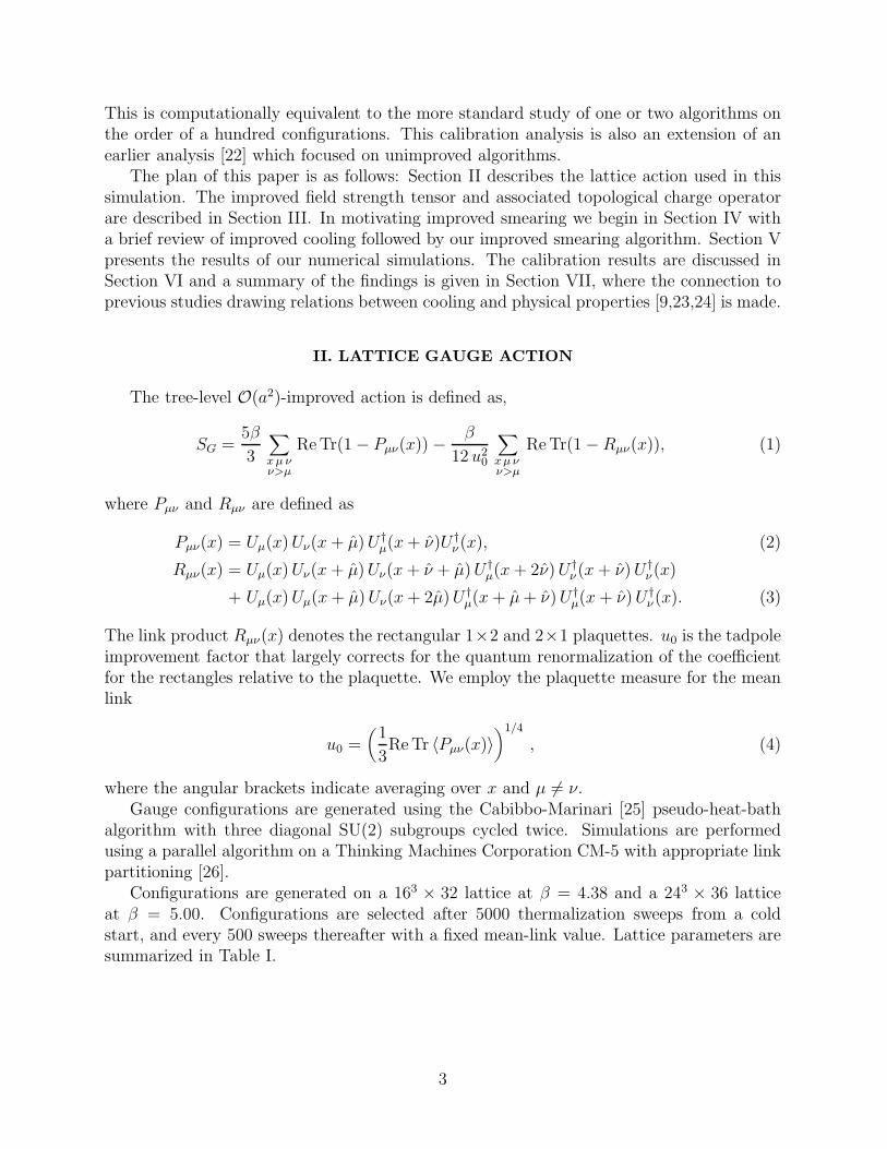
II. LATTICE GAUGE ACTION

The tree-level O(a2)-improved action is defined as,

SG =5β

3

∑

xµ νν>µ

ReTr(1− Pµν(x))−β

12 u20

∑

xµ νν>µ

ReTr(1−Rµν(x)), (1)

where Pµν and Rµν are defined as

Pµν(x) = Uµ(x)Uν(x+ µ)U †µ(x+ ν)U †

ν(x), (2)

Rµν(x) = Uµ(x)Uν(x+ µ)Uν(x+ ν + µ)U †µ(x+ 2ν)U †

ν(x+ ν)U †ν(x)

+ Uµ(x)Uµ(x+ µ)Uν(x+ 2µ)U †µ(x+ µ+ ν)U †

µ(x+ ν)U †ν(x). (3)

The link product Rµν(x) denotes the rectangular 1×2 and 2×1 plaquettes. u0 is the tadpoleimprovement factor that largely corrects for the quantum renormalization of the coefficientfor the rectangles relative to the plaquette. We employ the plaquette measure for the meanlink

u0 =(

1

3ReTr 〈Pµν(x)〉

)1/4

, (4)

where the angular brackets indicate averaging over x and µ 6= ν.Gauge configurations are generated using the Cabibbo-Marinari [25] pseudo-heat-bath

algorithm with three diagonal SU(2) subgroups cycled twice. Simulations are performedusing a parallel algorithm on a Thinking Machines Corporation CM-5 with appropriate linkpartitioning [26].

Configurations are generated on a 163 × 32 lattice at β = 4.38 and a 243 × 36 latticeat β = 5.00. Configurations are selected after 5000 thermalization sweeps from a coldstart, and every 500 sweeps thereafter with a fixed mean-link value. Lattice parameters aresummarized in Table I.

3

III. TOPOLOGICAL CHARGE OPERATOR

The topological charge of a gauge field configuration provides a particularly sensitiveindicator of the performance of various smoothing algorithms. The topological charge isrelated to the field strength tensor by

Q =∑

x

q(x) =∑

x

g2

32π2ǫµνρσTr (Fµν(x)Fρσ(x)) , (5)

where q(x) is the topological charge density. An expression for Fµν may be obtained byexpanding the definition of the Wilson loop. Consider a loop C in the µ-ν plane

Cµν(x) = P exp(

ig∮

CA(x) · dx

)

= P[

1 + ig(∮

CA(x) · dx

)

− g2

2!

(∮

CA(x) · dx

)2

+O(g3)

]

, (6)

The line integral is easily evaluated using Stokes theorem and a Taylor expansion of ∂µAν(x)about x0

∮

CA(x) · dx =

∫

dxµdxν

[

Fµν(x0) + (xµDµ + xνDν)Fµν(x0)

+1

2

(

x2µD

2µ + x2

νD2ν

)

Fµν(x0) +O(a2g2, a4)]

. (7)

The integration limits are determined by the size of the Wilson loop. Positioning the ex-pansion point x0 at the center of the Wilson loop one finds

∮

1×1A(x) · dx = a2Fµν(x0) +

a4

24

(

D2µ +D2

ν

)

Fµν(x0) + ... (8)

∮

2×1A(x) · dx = 2a2Fµν(x0) +

a4

12

(

4D2µ +D2

ν

)

Fµν(x0) + ... (9)

∮

1×2A(x) · dx = 2a2Fµν(x0) +

a4

12

(

D2µ + 4D2

ν

)

Fµν(x0) + .... (10)

Hence, Fµν may be extracted from consideration of the 1× 1 plaquette alone. To isolatethe second term of the expansion in Eq. (6), one takes advantage of the Hermitian natureof Fµν(x). Constructing Fµν(x) symmetrically about x leads to

g Fµν(x) =−i

8

[

(

O(1)µν (x)−O(1)†

µν (x))

− 1

3Tr

(

O(1)µν (x)−O(1)†

µν (x))

]

, (11)

TABLE I. Parameters of the numerical simulations.

Action Volume NTherm NSamp β a (fm) u0 Physical Volume fm

Improved 163 × 32 5000 500 4.38 0.165(2) 0.8761 2.643 × 5.28

Improved 243 × 36 5000 500 5.00 0.077(1) 0.9029 1.8483 × 2.772

4

U (x)x

µ

ν

µν

(1)O (x) =

µ

FIG. 1. Graphical representation of the link products summed in creating O(1)µν (x).

where O(1)µν (x) is the sum of 1× 1 Wilson loops illustrated in Fig. 1,

O(1)µν (x) = Uµ(x)Uν(x+ µ)U †

µ(x+ ν)U †ν(x)

+ Uν(x)U†µ(x+ ν − µ)U †

ν(x− µ)Uµ(x− µ)

+ U †µ(x− µ)U †

ν(x− µ− ν)Uµ(x− µ− ν)Uν(x− ν)

+ U †ν(x− ν)Uµ(x− ν)Uν(x+ µ− ν)U †

µ(x) . (12)

This well known definition for Fµν(x) is commonly employed in the Clover term of theSheikholeslami-Wohlert [27] improved quark action. Although, not everyone enforces thetraceless nature of the Gell-Man matrices by subtracting off the trace as in Eq. (11).

Unfortunately, this definition has large O(a2) errors. These errors are most apparent inthe topological charge. Even after hundreds of sweeps of cooling this simple definition failsto take on integer values. Errors are typically at the 10% level.

To improve the topological charge operator, we improve the definition of the field strengthtensor Fµν by removing O(a2) errors with a linear combination of plaquette and rectangleWilson loops

O(2)µν (x) = c1O(1)

µν (x) +c2u20

I(2)µν (x) , (13)

where the tadpole coefficient u0 is defined in Eq. (4). Here I(2)µν (x) is the link products of

1× 2 and 2× 1 rectangles in the µ-ν plane

I(2)µν (x) = Uµ(x)Uµ(x+ µ)Uν(x+ 2µ)U †

µ(x+ µ+ ν)U †µ(x+ ν)U †

ν(x)

+ Uµ(x)Uν(x+ µ)Uν(x+ µ+ ν)U †µ(x+ 2ν)U †

ν(x+ ν)U †ν (x)

+ Uν(x)Uν(x+ ν)U †µ(x− µ+ 2ν)U †

ν(x− µ+ ν)U †ν (x− µ)Uµ(x− µ)

+ Uν(x)U†µ(x− µ+ ν)U †

µ(x− 2µ+ ν)U †ν(x− 2µ)Uµ(x− 2µ)Uµ(x− µ)

+ U †µ(x− µ)U †

µ(x− 2µ)U †ν(x− 2µ− ν)Uµ(x− 2µ− ν)Uµ(x− µ− ν)Uν(x− ν)

+ U †µ(x− µ)U †

ν(x− µ− ν)U †ν(x− µ− 2ν)Uµ(x− µ− 2ν)Uν(x− 2ν)Uν(x− ν)

+ U †ν(x− ν)Uµ(x− ν)Uµ(x+ µ− ν)Uν(x+ 2µ− ν)U †

µ(x+ µ)U †µ(x)

+ U †ν(x− ν)U †

ν (x− 2ν)Uµ(x− 2ν)Uν(x+ µ− 2ν)Uν(x+ µ− ν)U †µ(x) , (14)

depicted in Fig. 2. The coefficients c1 and c2 are determined by combining Eqs. (8), (9)and (10) to remove O(a2) errors.

5

O (x) = xµ

µ

ν

µ

x

µ

ν

+ c1 2

U (x)(2)

µν

U (x)

c

FIG. 2. Graphical representation of the link products summed in creating O(2)µν (x).

a2 Fµν(x0) =5

3

[∮

1×1A(x) · dx

]

− 1

6

[∮

2×1A(x) · dx+

∮

1×2A(x) · dx

]

, (15)

indicating the coefficients for the O(a2)-improved Fµν of Eq. (13) are

c1 =5

3and c2 = −1

6. (16)

IV. COOLING AND SMEARING ALGORITHMS

In this section we motivate and introduce an improved version of APE smearing. Themotivation is based on improved cooling, and therefore we begin with a very brief overviewof cooling algorithms. Cooling consists of minimizing the local action effectively one link atthe time. The local action is that contribution to the action associated with a single link.

A. Improved Cooling

Standard cooling minimizes the local Wilson action associated with a link at each linkupdate. The local action associated with the link Uµ(x) is proportional to

Sl(x, µ) =∑

νν 6=µ

ReTr (1− Uµ(x)Σµν(x)) , (17)

where Σµν(x) is the sum of the two staples associated with Uµ(x) lying in the µ-ν plane

Σµν(x) = Uν(x+ µ)U †µ(x+ ν)U †

ν(x) + U †ν (x+ µ− ν)U †

µ(x− ν)Uν(x− ν) . (18)

The local action associated with the link Uµ(x) is minimized in standard cooling by a mini-mization process, i.e., by replacing the original link by the link Uµ(x) which optimizes

maxReTr

Uµ(x)∑

νν 6=µ

Σµν(x)

. (19)

6

Improved cooling proceeds in exactly the same manner, but with the plaquette-basedstaples replaced with the linear combination of plaquette-based staples and rectangle-basedstaples. For improved cooling we use

maxReTr

Uµ(x)∑

νν 6=µ

ΣIµν(x),

. (20)

Where

ΣIµν =

5

3Σµν +

1

12 u2o

ΣRµν , (21)

and

ΣRµν(x) = Uν(x+ µ)Uν(x+ ν + µ)U †

µ(x+ 2ν)U †ν(x+ ν)U †

ν(x)

+ Uµ(x+ µ)Uν(x+ 2µ)U †µ(x+ µ+ ν)U †

µ(x+ ν)U †ν (x)

+ Uν(x+ µ)U †µ(x+ ν)U †

µ(x+ ν − µ)U †ν(x− µ)Uµ(x− µ)

+ U †ν(x+ µ− ν)U †

ν(x+ µ− 2ν)U †µ(x− 2ν)Uν(x− 2ν)Uν(x− ν)

+ Uµ(x+ µ)U †ν(x+ 2µ− ν)U †

µ(x+ µ− ν)U †µ(x− ν)Uν(x− ν)

+ U †ν(x+ µ− ν)U †

µ(x− ν)U †µ(x− ν − µ)Uν(x− ν − µ)Uµ(x− µ) . (22)

The mean-field factor u0 is updated following each sweep through the lattice and rapidlygoes to 1 as perturbative tadpole contributions are removed. As we wish to study O(a2)–improved cooling, the coefficients are based on those of the action [17,28]. While this actionimproves contact with QCD, this choice of action does not completely stabilize instantonson the lattice [15,29]. Removal of O(a2) errors and stabilization of instantons requires theconsideration of additional loops [16,30]. The preferred algorithm for finding the Uµ(x) whichmaximizes Eq. (19) is based on the Cabbibo-Marinari [25] pseudo-heat-bath algorithm forconstructing SU(3) -color gauge configurations. There, operations are performed at theSU(2) level where the algorithm is transparent.

An element of SU(2) may be parameterized as, U = a0I + i~a · ~σ, where a is real anda2 = 1. Since sums of products of SU(2) matrices are proportional to SU(2) matrices,

∑

νν 6=µ

ΣIµν(x) = kUµ(x) , (23)

where Uµ(x) ∈ SU(2) and

k2 ≡ det

∑

νν 6=µ

ΣIµν(x)

. (24)

The maximum of the expression

ReTr

Uµ(x)∑

νν 6=µ

ΣIµν(x)

= ReTr(

k Uµ(x)Uµ(x))

, (25)

7

is achieved when

ReTr(

Uµ(x)Uµ(x))

= ReTr(I) , (26)

which requires the link to be updated as

Uµ(x)→U ′µ(x) = U

−1µ (x) = U

†

µ(x) =

∑

νν 6=µ

ΣIµν(x)

k

†

. (27)

At the SU(3) level, we successively apply this algorithm to the three diagonal SU(2) sub-groups of SU(3) [25].

When considering an improved cooling algorithm it is crucial to loop over sufficient SU(2)subgroups to ensure that the subtle effects of the higher dimension operators introduced inimproving the action are reflected in the final SU(3) link. It is easy to imagine that only twoor three SU(2) subgroups may not take the SU(3) link close enough to the optimal link forthe effects of improvement to be properly seen. We find consideration of the three diagonalSU(2) subgroups looped over twice to be optimal. In fact we have seen round off errorsactually increase the action if too many loops are made.

The u0 factor of Eq. (21) is not held fixed during the improved cooling iteration. Startingfrom the value determined during the thermalization process, u0 is updated after every sweepthrough the lattice. After a few sweeps of improved cooling the value quickly converges to1 which is a good indication that short distance tadpole effects are being removed in thesmoothing procedure.

Finally it must be understood that cooling proceeds effectively one link at a time. Thatis, links involved in constructing ΣI

µν(x) are not updated simultaneously with Uµ(x). In factit is a nontrivial task identifying which links can be simultaneously updated on a massivelyparallel computer [26].

B. Improved Smearing

In this section we consider the APE smearing [1] algorithm. We extend this algorithmto produce an improved version, motivated by the success of the improved cooling program.

1. Reunitarization of the Links

APE smearing is a gauge equivariant1 [32] prescription for smearing a link Uµ(x) with itsnearest neighbors Uµ(x + ν), where ν is transverse to µ. The APE smearing process takesthe form

1Gauge equivariance means that if two starting gauge configurations are related by a gauge

transformation then the respective smeared configurations are also related by the same gauge

transformation.

8

Uµ(x) −→ U ′µ(x) = (1− α)Uµ(x) +

α

6

∑

νν 6=µ

Σ†µν(x) , (28)

Uµ(x) = PU ′µ(x) , (29)

where Σµν(x) is the sum of the two staples associated with Uµ(x) defined in Eq. (18) and Pis a projection operator which projects the smeared link back onto SU(3).

The reunitarization procedure is of central importance when smearing is applied to thegauge links because the APE smearing operation produces links outside the SU(3) gaugegroup in the intermediate stage of smearing. The link between smearing and cooling isestablished via the manner in which smeared links are projected back onto SU(3). Thepreferred approach is to select the link variable Uµ(x) that maximizes the quantity

ReTr(

Uµ(x)U′†µ (x)

)

. (30)

In this case a clear connection to cooling is established when α → 1 as

maxReTr(

Uµ(x)U′†µ (x)

)

= maxReTr

Uµ(x)∑

νν 6=µ

Σµν(x)

, (31)

which is precisely the condition of Eq. (19) for cooling. In other words, projection of thesmeared link back onto the gauge group via Eq. (31) selects the link which minimizes thelocal action. Improvement of the staple based on the action will aid in removing O(a2)errors encountered in the SU(3) projection. In practice, the same Cabibbo-Marinari-basedcooling method of operating on SU(2) subgroups may be used to obtain the ultimate SU(3)link.

However there is one very important difference remaining between APE smearing andcooling. While cooling effectively updates one link at a time, feeding the smoothed linkimmediately into the next link update, APE smearing proceeds uniformly with all linksbeing simultaneously updated. Smoothed links are not introduced into the algorithm untilthe next iteration of the APE smearing process takes place.

It is this latter point that provides the form factor interpretation of APE smearing infat-link fermion actions [4]. There smearing can be understood to introduce a form factorsuppressing the coupling of gluons to quarks at the edge of the Brillouin zone where latticeartifacts are most problematic. The form factor analysis restricts the smearing fraction tothe range 0 ≤ α ≤ 3/4. Indeed in practice, smearing fractions beyond 3/4 do not lead tosmooth gauge configurations.

2. Improving Smearing

Having made firm contact with cooling it is clear that replacing the simple staple ofEq. (18) with the improved staple of Eq. (21) may lead to a realization of the benefits ofimproved cooling within APE smearing. Hence we define improved smearing to be an APEsmearing step in which

9

Uµ(x) −→ U ′µ(x) = (1− α)Uµ(x) +

α

6

∑

νν 6=µ

ΣI†(x)µν , (32)

Uµ(x) = PU ′µ(x) , (33)

where ΣIµν(x) is the improved staple of Eq. (21).

Signatures of improvement include the preservation of structures in the action densitydistribution under smearing. O(a2) errors in the standard Wilson action act to underesti-mate the local action and destroy topologically nontrivial field configurations [15]. Improvedsmearing will have reduced O(a2) errors and hence better preserve topologically nontrivialfield configurations. Hence an associated signature of improvement is the stability of topo-logical charge under hundreds of smearing sweeps. Of course, one could alter the coefficientsof the improvement terms to stabilize instantons [15] at the expense of introducing O(a2)errors into the smoothing action.

The extended nature of the staple will alter the stability range of α. Where standardAPE smearing provides the range 0 ≤ α ≤ 3/4, we find the upper stability limit lies belowα = 0.6.

V. NUMERICAL SIMULATIONS

We analyze two sets of gauge field configurations generated using the Cabibbo-Marinari [25] pseudo-heat-bath algorithm with three diagonal SU(2) subgroups looped overtwice. Details may be found in Table I. As discussed in the introduction, analysis of a fewconfigurations proves to be sufficient to resolve the nature of the algorithms under investiga-tion. We consider eleven 163 × 32 configurations and six 243 × 36 configurations. For eachconfiguration we separately perform 200 sweeps of cooling and 200 sweeps of improved cool-ing. We explore 200 sweeps of APE smearing at seven values of the smearing fraction and200 sweeps of improved smearing at five values of the smearing fraction. For APE smearingwe consider α = 0.10, 0.20, 0.30, 0.40, 0.50, 0.60, and 0.70. Similarly for improved smearingwe consider α = 0.10 to 0.50 at intervals of 0.10. The extended nature of the staple altersthe stability range of α to lie below α = 0.6.

For clarity, we define the number of times an algorithm is applied to the entire latticeas nc, nIc, nape(α) and nIape(α) for cooling, improved cooling, APE smearing and improvedsmearing respectively. We monitor both the total action normalized to the single instantonaction S0 = 8π2/g2 and the topological charge operators, QL and QImp

L , from which weobserve their evolution as a function of the appropriate sweep variable and smearing fractionα.

A. The Influence Of The Number Of Subgroups On The Gauge Group.

In this section we describe the influence of including additional SU(2) subgroups in con-structing the gauge group SU(3) and explore the impact it has on the smoothing procedure.The Cabibbo-Marinari algorithm [25] constructs the SU(N) gauge groups using SU(2) sub-groups. It is understood that the minimal set required to construct SU(3) matrices is two

10

FIG. 3. The evolution of the topological charge estimated by the improved operator as a func-

tion of standard cooling sweeps nc for various numbers of SU(2) subgroups. The curves are for

a typical configuration from the 163 × 32 lattices where a = 0.165(2) fm. The parameter cycle

describes the number of times the three diagonal SU(2) subgroups are cycled over.

diagonal SU(2) subgroups. After having performed cooling on gauge field configurationswe noticed that the resulting cooled gauge field configurations were not smooth even aftera large number of smoothing steps. Adding a third SU(2) subgroup made a significantdifference in the resulting smoothness.

We explored further by simply performing additional cycles, ncycle, around the threediagonal SU(2) subgroups. We monitored the smoothing rate using both the StandardWilson and the improved action according to the cycle number being set to ncycle = 1, 2 and3. Based on the evolution of the action, we found that the optimum cooling rate on gaugefield configurations is achieved using the three diagonal SU(2) subgroups cycled over twice,ncycle = 2. Cycling more than twice provides very little further reduction of the action andround off errors may actually increase the action on occasion. Hence two cycles over the threediagonal SU(2) subgroups is sufficient to precisely create the SU(3) link which minimizesthe local action. This determination is crucial to ensuring the effects of our improved actionare fully reflected in the SU(3) link.

We also monitored the evolution of the topological charge with respect to the abovenumber of cycles. On the 163 × 32 lattice with spacing of a = 0.165(2) fm, we observe adisagreement of the trajectories for the topological charge for different numbers of the SU(2)subgroups cycles. Fig. 3 displays results for standard cooling and Fig. 4 displays similarresults for improved cooling. A comparison of Figs. 3 and 4 indicates the trajectories alsodiffer between cooling and improved cooling.

Hence we see subtle differences in the algorithms leading to dramatic differences in thetopological charge. One must conclude that a lattice spacing of 0.165(2) fm is too coarse for

11

FIG. 4. The evolution of the topological charge estimated by the improved operator as a func-

tion of improved cooling sweeps nIc for various numbers of cycles over the three diagonal SU(2)

subgroups. The curves are for the same configuration illustrated in Fig. 3.

a serious study of topology in SU(3) gauge fields using the algorithms considered here. Thedifficulty lies in the fact that the algorithms have a dislocation threshold typically a little overtwo lattice spacings [16,21]. Instantons with a size smaller than the dislocation threshold areremoved during the process of smoothing. While this threshold has the desireable property ofremoving lattice artifacts, we note that twice the lattice spacing is 0.33 fm. Minor differencesin the dislocation thresholds of the various algorithms will cause some (anti)instantons tosurvive under one algorithm where they are removed under another.

On the other hand, a lattice spacing the order of 0.077(1) fm appears to allow a mean-ingful study of topology in SU(3) gauge theory. Twice this lattice spacing is 0.15 fm, wellbelow the typical size of instantons [24].

We also note here the accuracy with which our improved topological charge operatorreproduces integer values. These results should be contrasted with the usual 10% errors ofthe unimproved operator at similar lattice spacings. Such errors on a topological charge of5 can lead to the uncomfortable result of Q ≃ 4.5 when the unimproved operator is used.

With the finer 243 × 36 lattice at β = 5.00, we observe perfect agreement among trajecto-ries for different numbers of cycles of the three SU(2) subgroups. Moreover, the topologicalcharge remains stable for hundreds of sweeps following the first three sweeps. Figures 5and 6 compare the topological charge evolution for cooling versus improved cooling for sixconfigurations. In every case, the two algorithms produce the same topological charge for agiven configuration.

12

FIG. 5. The evolution curve for the topological charge estimated via the improved operator as

a function of cooling sweeps nc for six configurations on the 243 × 36 lattices at β = 5.00 where

a = 0.077(1) fm.

FIG. 6. The evolution curve for the topological charge estimated via the improved operator as

a function of improved cooling sweeps nIc for the same six configurations from the 243 × 36 lattices

at β = 5.00 illustrated in Fig. 5.

13

FIG. 7. The ratio S/S0 as a function of standard cooling sweeps nc for five configurations on

the 243 × 36 lattice at β = 5.0. The single instanton action is S0 = 8π2/g2.

B. The Action

We begin by considering the action evolution on both lattices. Here we report the actiondivided by the single instanton action S0 = 8π2/g2. It is important to note that althoughthe 243 × 36 lattice has almost four times more lattice sites than the 163 × 32 lattice, thephysical volume is smaller by almost a factor of three. As such the typical topological chargesencountered are smaller in magnitude.

Figs. 7, 8, 9, and 10 report the typical evolution of the action under standard cooling,improved cooling, APE smearing and improved smearing respectively. Inspection of thefigures reveals that improved cooling preserves the action better than standard cooling overa couple hundred sweeps. As expected, standard APE smearing remains slower than coolingor improved cooling even at our most efficient smearing fraction (α = 0.70). Similar resultsare observed for improved smearing at our most efficient smearing fraction of α = 0.50 inFig. 10.

Based on these observations, one concludes that the fastest way to remove the short rangequantum fluctuations on an O(a2) gauge field configuration, is through standard cooling,which lowers the action more rapidly than improved cooling as a function of cooling sweep.In turn we see that improved cooling is faster than the maximum stable standard APEsmearing, which is faster than the maximum stable improved smearing. This is illustrated byFigs. 7–10. It is important to emphasize that the fastest way of removing these fluctuationsis not necessarily the best as far as the topology is concerned. It is already established thatthe O(a2) errors of the standard Wilson action act to underestimate the action [15]. Theseerrors spoil instantons which might otherwise survive under improved cooling.

14

FIG. 8. The ratio S/S0 as a function of improved cooling sweeps nIc for five configurations on

the 243 × 36 lattice at β = 5.0. The rate of cooling is seen to be somewhat slower than that for

the standard cooling.

FIG. 9. The ratio S/S0 as a function of APE smearing sweeps nape(α) for one configuration

on the 243 × 36 lattice at β = 5.0. Each curve has an associated smearing fraction α. The rate of

lowering the action for the maximum stable smearing fraction (≈ 0.75) is seen to be less than that

for the other standard or improved cooling.

15

FIG. 10. The ratio S/S0 as a function of improved smearing sweeps nIape(α) for one configu-

ration on the 243 × 36 lattice at β = 5.0. Each curve has an associated smearing fraction α. We

see that this is the slowest of the four algorithms for lowering the action as a function of the sweep

number.

C. Topological Charge from Cooling and Smearing

We begin by considering the 163 × 32 lattices having a lattice spacing of a = 0.165(2)fm. In Fig. 11, we plot the evolution curve for the improved topological charge as a functionof the cooling sweep number, nc, for six of our configurations. Similarly in Fig. 12, for thesame six configurations we plot the improved topological charge operator but this time asa function of improved cooling sweep nIc. The line types in Figs. 11 and 12 correspond tothe same underlying configurations and are to be directly compared. For example, the solidcurve corresponds to the same gauge field configuration in both figures but with a differentalgorithm applied to it. From these two figures we notice the two cooling methods lead tocompletely different values for the topological charge.

Improved cooling brings stability to the evolution of the topological charge whereasstandard cooling gives rise to numerous fluctuations to the topological charge. For improvedcooling, plateaus appear after about forty sweeps and persist for hundreds of sweeps. Thisis a celebrated feature of improved cooling.

This algorithmic sensitivity of the topological charge is also seen in Figs. 13 and 14, forAPE and improved smearing on a single configuration (the solid line of Figs. 11 and 12).Within APE smearing or improved smearing, the topological charge trajectories follow simi-lar patterns but different rates for various smearing fractions. However, APE smearing leadsto values for the topological charge which are different from that obtained under improvedsmearing. An important point is that improved smearing stabilizes the topological chargeat 95 sweeps for α = 0.5, whereas standard smearing shows no sign of stability until 140

16

FIG. 11. QImpL versus nc for six configurations on the 163 × 32 lattices at β = 4.38, a = 0.165(2)

fm. Each line corresponds to a different configuration.

FIG. 12. QImpL versus nIc for six configurations on the 163 × 32 lattices. The different line types

identifying different configurations match the configurations identified in Fig. 11.

17

FIG. 13. The evolution of QImpL using APE smearing as a function of APE smearing sweep

nape(α) on the 163 × 32 lattice at β = 4.38. Here different line types correspond to different

smearing fractions.

iterations at α = 0.5. Hence we see significant improvement in the topological aspects ofthe gauge field configurations under improved smearing.

On our finer lattice, we find a completely different behavior for the topological chargeevolution. The topological charge is established very quickly; after a few sweeps in the caseof cooling or improved cooling as illustrated in Figs. 5 and 6. The topological charge persistswithout fluctuation for hundreds of sweeps, both for cooling and for smearing as illustratedin Figs. 15 and 16 for APE and improved smearing respectively. Moreover, the topologicalcharge is independent of the smearing algorithm.

These results are to be compared with Fig. 11 and Fig. 12, where transitions are observedeven with improved cooling on the coarser lattice with a = 0.165(2) fm. The results on ourfine lattice suggest the characteristic size of instantons is much larger than the dislocationthreshold, such that the topological structure of the gauge fields is smooth at the scale ofthe threshold.

In Fig. 15 for standard APE smearing we observe a slower convergence to integer topo-logical charge than in Fig. 16 for improved smearing when 0.1 ≤ α ≤ 0.5. This featureof improved smearing is illustrated in detail in Fig. 17. However, APE smearing has theadvantage to allow values for the smearing fraction up to α = 0.70 which cannot be accessedby improved smearing.

Having demonstrated that it is possible to precisely match the behavior of the algorithmson fine lattice spacings, we proceed to calibrate the efficiency of these algorithms in thefollowing section.

18

FIG. 14. The evolution of QImpL using improved smearing as a function of APE smearing sweep

nIape(α) on the 163 × 32 lattice at β = 4.38. Here different line types correspond to different

smearing fractions.

FIG. 15. The evolution of QImpL using APE smearing as a function of APE smearing sweep

nape(α) on the 243 × 36 lattice at β = 5.00. Here different line types correspond to different

smearing fractions.

19

FIG. 16. The evolution of QImpL using APE smearing as a function of APE smearing sweep

nIape(α) on the 243 × 36 lattice at β = 5.00. Here different line types correspond to different

smearing fractions.

FIG. 17. The evolution of the improved topological charge, QImpL , as a function of standard

APE smearing sweeps, nape(α), for 0.1 ≤ α ≤ 0.7 (solid lines) is compared to improved smearing

sweeps, nIape(α), (dotted-dashed lines) for the same smearing fractions 0.1 ≤ α ≤ 0.5 on the

243 × 36 lattice at β = 5.00. The horizontal dotted-dashed line is QImpL = −4.

20

VI. SMOOTHING ALGORITHM CALIBRATION

Here we calibrate the relative rate at which quantum fluctuations are removed fromtypical field configurations by the various algorithms. The calibration is done using theaction normalized to the single instanton action, S/S0, on both, the 163 × 32 lattices and243 × 36 lattices. The action normalized to the single instantons action, S/S0, is of particularinterest because it provides insight into the lattice content as well as the rate at which thequantum fluctuations are removed.

While there is no doubt that the algorithms may be accurately calibrated on the fine243 × 36 lattice, the 163 × 32 lattice with a = 0.165(2) fm presents more of a challenge. Asa result, in most cases we will show the graphs produced from the 163 × 32 lattice analysisand simply present the numerical results for both the 163 × 32 and 243 × 36 lattices.

The numerical results are summarized in Tables II, III, and VI for the 163 × 32 latticesand in Tables IV, V, and VII for the 243 × 36 lattices.

A. APE Smearing and Improved Smearing Calibration.

To calibrate the rate at which the algorithm reduces the action we record the nearestnumber of sweeps required to reach a given threshold in S/S0. The action thresholds arespaced logarithmically to obtain a uniform distribution in the number of sweeps required toreach a threshold. The relative rates of smoothing are established by comparing the relativenumber of sweeps required to reach a particular threshold.

Here we calibrate the APE smearing algorithm characterized by the smearing fractionα and the number of smearing iterations nape(α). The different threshold crossings arecharacterized by the number of sweeps required to reach that threshold, nape(α). In Fig. 18we show the number of sweeps required to reach a threshold when α = 0.5, nape(0.50),relative to that required for other α values, nape(α). We plot these relative smoothingrates as a function of nape(α) such that low S/S0 thresholds are reached after hundreds ofiterations of the smoothing algorithm. Fig. 19 shows similar results for improved smearing.In these figures and in the following analysis, we omit thresholds that result in fewer thanfive smoothing iterations as these points produce integer discretization errors of more than20%.

Both standard and improved smearing algorithms have a relative smoothing rate whichis independent of the amount of smoothing done. By calculating the average value for eachof the bands in Figs. 18 and 19, we can investigate the dependence of the average relativesmoothing rate 〈nape(0.50)/nape(α)〉 on α.

Fig. 20 illustrates a linear fit to the data constrained to pass through the origin. We find〈nape(0.50)/nape(α)〉 = 2.00α such that

nape(α′)

nape(α)=

α

α′(34)

in agreement with our earlier analysis [22]. The extent to which this relationship holds canbe verified [22] by plotting the ratio α′nape(α

′)/αnape(α) and comparing the results to 1.

21

FIG. 18. The ratio nape(0.50)/nape(α) versus nape(α) for numerous S/S0 thresholds on the

163 × 32 lattice at β = 4.38. From top to bottom the data point bands correspond to α = 0.7, 0.6,

0.5, 0.4, 0.3, 0.2, and 0.1.

FIG. 19. The ratio nIape(0.50)/nIape(α) versus nIape(α) for numerous S/S0 thresholds on the

163 × 32 lattice at β = 4.38. From top to bottom the data point bands correspond to α = 0.5, 0.4,

0.3, 0.2, and 0.1.

22

FIG. 20. Illustration of the dependence of 〈nape(0.50)/nape(α)〉 for APE smearing on the smear-

ing fraction α. The solid line is a linear fit to the data constrained to pass through the origin.

In plotting the band averages for the improved smearing algorithm of Fig. 19 in Fig. 21,one finds a small deviation of the points from the line y = 2α. This suggests that Eq. (34)is not sufficiently general for the improved smearing case.

A better approximation to establish the α dependence, that is similar to Eq. (34) andcontains Eq. (34) is

nIape(α′)

nIape(α)=

(

α

α′

)δ

, (35)

where δ is equal to one in the case of standard APE smearing and can deviate away fromone for improved smearing.

In Fig. 22, the logarithm of Eq. (35) is plotted. The slope of the data provides δ =0.914(1) for both the 163 × 32 and the 243 × 36 lattices. We also verified δ = 1.00 for theAPE smearing data. Fig. 23 plots the ratio of the left- and right-hand sides of Eq. (35) asa function of nIape(α) for α

′ > α. The ratio is one as expected with 5% for large amountsof smearing where integer discretization errors are minimized. Throughout the followinganalysis, δ is fixed at 0.914(1).

B. APE and Improved smearing cross calibration.

In this section we focus on the cross calibration of the smearing algorithms. In Fig. 24,we compare the number of improved smearing sweeps required to reach a threshold for var-ious improved smearing fractions relative to APE smearing at α = 0.5. The lowest bandcorresponds to an improved smearing fraction of 0.10. From this, we conclude that for low

23

FIG. 21. Illustration of the dependence of < nIape(0.50)/nIape(α) > for APE smearing on the

improved smearing fraction α. The solid line fit is constrained to pass through the origin.

FIG. 22. Illustration of the dependence of ln (< nIape(0.50)/nIape(α) >) on the improved smear-

ing fraction α for improved smearing. The solid line fit indicates δ = 0.914.

24

FIG. 23. Illustration of the degree to which the relation Eq. (35) is satisfied for improved

smearing. Here the entire data set is plotted for α and α′ = 0.5, 0.4, 0.3, 0.2 and 0.1. Data are

from 163 × 32 lattice at β = 4.38.

α values APE smearing and improved smearing produce roughly equivalent smeared config-urations. However, there are some evident differences in the rate at which both algorithmsperform. For intermediate to large α there is curvature in the bands. Early in the smear-ing process, fewer sweeps of improved smearing are required to reach a threshold. That is,improved smearing removes action faster than APE smearing in the early stages of smear-ing. This behavior is also manifest in the analogous results for the fine 243 × 36 lattice.As emphasized in the discussion surrounding Fig. 17, improved smearing also provides atopological charge closer to an integer than APE smearing. Together, these two propertiesof improved smearing identify a genuine improvement in the smearing process.

For the coarse 163 × 32 lattice data, the bands are thick for large smearing fractions indi-cating improved smearing does perform significantly different from standard APE smearing.Contributions from individual configurations are clearly visible as lines within the bands.This structure is due to the coarse lattice spacing of 0.165(2) fm which reveals differencesbetween the algorithms. Such structure is not seen in the fine 243 × 36 lattice results. Therea precise calibration is possible.

In Tables II and III, we report the averages of each band for APE and improved smearingon the 163 × 32 lattices. In Tables IV and V we report similar results for the 243 × 36 lattices.

Based on equations Eq. (34) and Eq. (35) for APE and improved smearing, we expect

α′nape(α′)

αδnIape(α)= constant . (36)

This ratio is plotted in Fig. 25 where a rather mild dependence on nIape(α) is revealed.Averaging these results provides 0.81(2) for the constant of Eq. (36). Similar results are

25

FIG. 24. The ratio nape(0.50)/nIape(α) versus nIape(α) for numerous threshold actions on the

163 × 32 lattice at β = 4.38. From top to bottom the data point bands correspond to improved

smearing fractions α = 0.5, 0.4, 0.3, 0.2, and 0.1.

TABLE II. The averages of the ratios < nape(0.50)/nape(α) > and < nIape(0.50)/nape(α) > for

various smearing fractions α from the 163 × 32 lattice at β = 4.38.

α for APE smearing

0.10 0.20 0.30 0.40 0.50 0.60 0.70

nape(0.50) 0.195(1) 0.394(2) 0.595(3) 0.797(4) 1.0 1.203(1) 1.407(1)

nIape(0.50) 0.227(1) 0.465(1) 0.706(1) 0.948(1) 1.189(1) 1.431(1) 1.673(1)

TABLE III. The averages of the ratios < nape(0.50)/nIape(α) > and < nIape(0.50)/nIape(α) >

for various smearing fractions α from the 163 × 32 lattice at β = 4.38.

α for improved smearing

0.10 0.20 0.30 0.40 0.50

nape(0.50) 0.196(1) 0.376(3) 0.543(1) 0.697(1) 0.842(1)

nIape(0.50) 0.228(1) 0.442(1) 0.641(1) 0.827(1) 1.0

TABLE IV. The averages of the ratios < nape(0.50)/nape(α) > and < nIape(0.50)/nape(α) >

for various smearing fractions α from the 243 × 36 lattice at β = 5.00.

α for APE smearing

0.10 0.20 0.30 0.40 0.50 0.60 0.70

nape(0.50) 0.195(1) 0.395(1) 0.595(1) 0.797(1) 1.0 1.205(1) 1.410(1)

nIape(0.50) 0.227(1) 0.462(1) 0.698(1) 0.937(1) 1.176(1) 1.416(1) 1.658(1)

26

TABLE V. The averages of the ratios < nape(0.50)/nIape(α) > and < nIape(0.50)/nIape(α) >

for various smearing fractions α from the 243 × 36 lattice at β = 5.00.

α for improved smearing

0.10 0.20 0.30 0.40 0.50

nape(0.50) 0.196(1) 0.378(1) 0.546(1) 0.704(1) 0.851(1)

nIape(0.50) 0.228(1) 0.442(1) 0.641(1) 0.826(1) 1.0

FIG. 25. Illustration of the degree to which the relation Eq. (36) is satisfied for calibration of

the action under APE and improved smearing. Here the entire data set is plotted.

seen for the finer 243 × 36 lattice, but with greater precision in the calibration reflected in anarrower band. There the constant is also 0.81(2). However, it should also be noted that forα ≤ 0.5, improved smearing achieves integer topological charge faster than standard APEsmearing.

C. Calibration of Cooling and Smearing

In this section we apply the ansatz of equations Eq. (34) and Eq. (35) to relate thecooling and smearing algorithms. Fig. 26 displays results comparing cooling and standardAPE smearing. For α as small as 0.1 it takes about 75 sweeps of APE smearing comparedwith 5 sweeps of cooling to arrive at an equivalent action. On the other end of the smearingfraction spectrum, we note the bands become very thick.

The calibration of these ratios indicates

nc

αnape(α)= 0.59(1), (37)

27

FIG. 26. The ratio nc/nape(α) versus nape(α) for numerous action thresholds for the 163 × 32

lattice at β = 4.38. From top down the data point bands correspond to α = 0.7, 0.6, 0.5, 0.4, 0.3,

0.2, and 0.1.

in agreement with that obtained in [22] where the analysis was performed on unimprovedgauge configurations. The reduction in O(a2) errors in the gauge field action affect bothalgorithms similarly such that the calibration of the relative smoothing rates remains unal-tered.

Further broadening of the bands is observed when comparing improved cooling withAPE smearing as illustrated in Fig. 27. The precision of improved cooling relative to APEsmearing leads to very different smoothed configurations at this coarse lattice spacing of0.165(2) fm. This indicates the algorithms are sufficiently different, that an accurate andmeaningful calibration is impossible.

This effect is not observed when we pass to our fine lattice spacing as displayed in Fig. 28.We remind the reader that the thickness of the band for small numbers of smoothing sweepsis simply due to the ratio of small integers taken in plotting the y-axis values.

The real test of improved smearing is the extent to which the algorithm can preserveaction associated with topological objects and thus maintain better agreement with moreprecise algorithms including cooling and improved cooling. Fig. 29 displays results for thecalibration of improved cooling with improved smearing. Comparing these results for eachsmearing fraction, α, with that for improved cooling and standard smearing in Fig. 27reveals that the improved smearing algorithm, which was seen to be better than standardAPE smearing algorithm does not perform as well as the improved cooling algorithm.

Similar results are seen in Fig. 30 where standard cooling is compared with improvedsmearing. Hence the annealing of the links in the process of cooling, where cooled links areimmediately passed into the determination of the next cooled link, is key to the precisionwith which cooling can preserve topological structure.

28

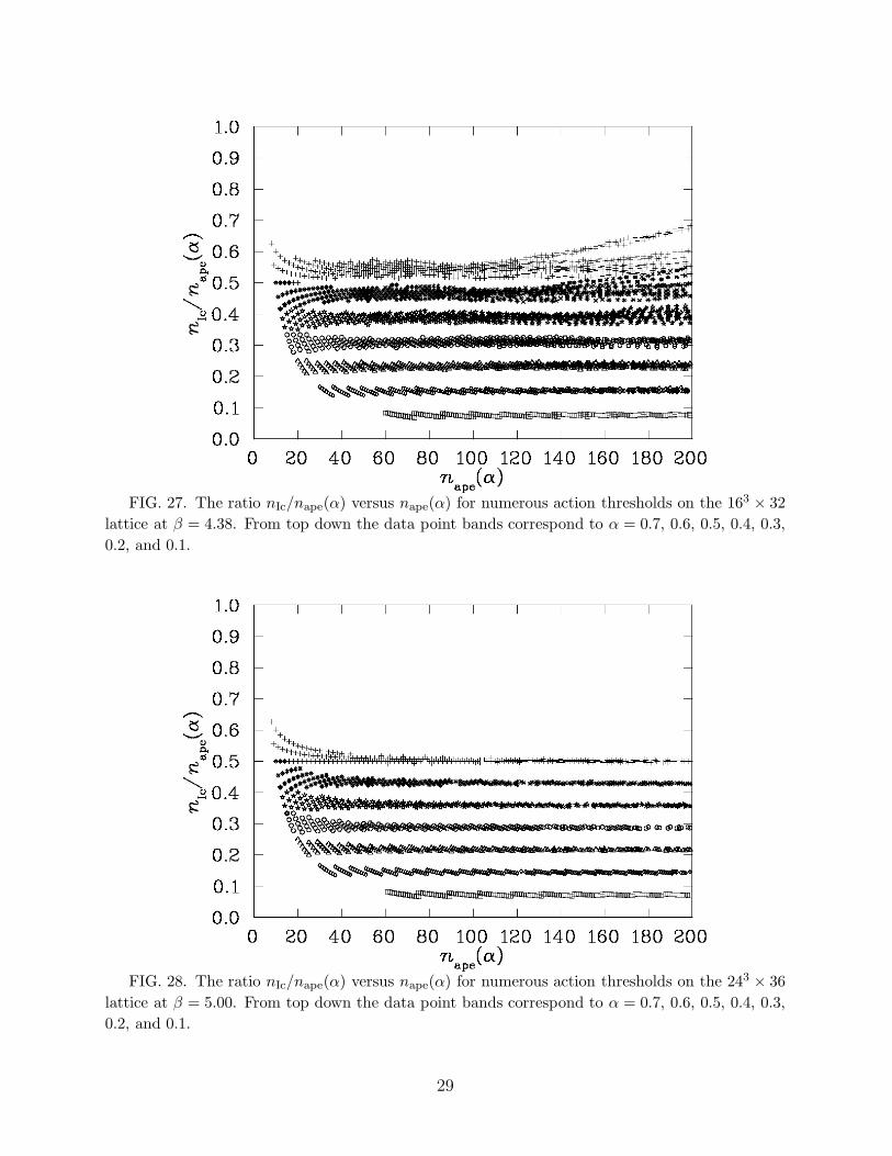
FIG. 27. The ratio nIc/nape(α) versus nape(α) for numerous action thresholds on the 163 × 32

lattice at β = 4.38. From top down the data point bands correspond to α = 0.7, 0.6, 0.5, 0.4, 0.3,

0.2, and 0.1.

FIG. 28. The ratio nIc/nape(α) versus nape(α) for numerous action thresholds on the 243 × 36

lattice at β = 5.00. From top down the data point bands correspond to α = 0.7, 0.6, 0.5, 0.4, 0.3,

0.2, and 0.1.

29

FIG. 29. The ratio nIc/nIape(α) versus nIape(α) for numerous action thresholds on the 163 × 32

lattice at β = 4.38. From top down the data point bands correspond to α = 0.5, 0.4, 0.3, 0.2, and

0.1.

FIG. 30. The ratio nc/nIape(α) versus nIape(α) for numerous action thresholds on the 163 × 32

lattice at β = 4.38. From top down the data point bands correspond to α = 0.5, 0.4, 0.3, 0.2, and

0.1.

30

TABLE VI. Calibration coefficients for various smoothing algorithms on the 163 × 32 lattice at

β = 4.38. Entries describe the relative smoothing rate for the algorithm ratio formed by selecting

an entry from the numerator column and dividing it by the heading of the denominator columns.

For example equation Eq. (37) corresponds to the first column of the third row.

Denominator

Numerator αnape(α) αδnIape(α) nc nIc

α′ nape(α′) 1.00(2) 0.81(2) 1.69(3) 1.30(2)

α′δnIape(α′) 1.25(3) 1.01(2) 2.13(5) 1.61(3)

nc 0.59(1) 0.47(1) 1 0.75(1)

nIc 0.77(1) 0.62(1) 1.33(2) 1

TABLE VII. Calibration coefficients for various smoothing algorithms on the 243 × 36 lattice

at β = 5.00. Entries describe the relative smoothing rate for the algorithm ratio formed by selecting

an entry from the numerator column and dividing it by the heading of the denominator columns.

For example equation Eq. (36) corresponds to the second column of the first row.

Denominator

Numerator αnape(α) αδnIape(α) nc nIc

α′ nape(α′) 1.00(2) 0.81(2) 1.64(2) 1.37(1)

α′δnIape(α′) 1.25(3) 1.01(2) 2.04(4) 1.67(3)

nc 0.611(9) 0.49(1) 1 0.84(1)

nIc 0.734(8) 0.60(1) 1.19(1) 1

Calibration of the smoothing rates as measured by the action for the algorithms un-der investigation are summarized in Tables VI and VII. The entries describe the relativesmoothing rate for the algorithm ratio formed by selecting an entry from the numerator col-umn and dividing it by the heading of the denominator columns. The entry comparing APEsmearing with itself reports the level to which the ansatz of equation Eq. (34) is satisfied.Similarly the entry comparing improved smearing with itself reports the level to which theansatz of equation Eq. (35) is satisfied.

D. Cooling versus Improved cooling.

Figure 31 reports a comparison of standard cooling with improved cooling on elevenconfigurations from the coarse 163 × 32 lattice. There the ratio nc/nIc < 1 confirms theexpectation that standard cooling does not preserve action on the lattice as well as theO(a2)-improved cooling. Fewer standard cooling sweeps are required to reach the sameaction threshold. Calibration of the algorithms appears plausible for the first 80 sweeps ofimproved cooling, after which the two algorithms smooth the configurations in very differentmanners. Any calibration at this lattice spacing is only very approximate beyond 80 sweepsof improved cooling where distinct configuration-dependent trajectories become visible. Thisresult is contrasted by the analogous analysis on our fine 243 × 36 lattice illustrated inFig. 32. While nc/nIc remains less than one, it is closer to one here than for the coarser

31

FIG. 31. The ratio nc/nIc versus nIc for numerous action thresholds on the 163 × 32 lat-

tice at β = 4.38. The significant differences between the algorithms are revealed by the

gauge-configuration dependence of the trajectories.

lattice as one might expect.

VII. CONCLUSIONS

We have introduced an improved version of the APE smearing algorithm founded onthe connection between cooling Eq. (19) and the projection of the APE smeared link backto the SU(3) gauge group via Eq. (31). This connection motivates the use of additionalextended paths combined with the standard “staple” as governed by the action to reducethe introduction of O(a2) errors in the smearing projection process.

Clear signs of improvement are observed. For a given smearing fraction α defined inequation (28), improved smearing preserves the action better than standard APE smearing ateach smearing sweep. At the same time improved smearing brings the improved topologicalcharge to an integer value faster than standard APE smearing.

The extended nature of the “staple” in improved smearing reduces the stability regime forthe smearing fraction. We found the improved smearing algorithm to be stable for α ≤ 0.5.At α = 0.6 the algorithm is unstable whereas standard APE smearing remains stable forα ≤ 0.75.

Given the wide variety of smoothing algorithms under investigation in the field of latticegauge theory, we have cross calibrated the speed with which the algorithms remove actionfrom the field configurations. In particular we have cross calibrated the smoothing rates ofAPE smearing at seven values of the smearing fraction; improved smearing at five values ofthe smearing fraction; cooling; and improved cooling. We explored smearing fractions in 0.1

32

FIG. 32. The ratio nc/nIc versus nIc for numerous action thresholds on the 243 × 36 lattice at

β = 5.00.

intervals starting at α = 0.1.The calibration has been investigated over a range of 200 sweeps for each smearing

algorithm on O(a2)-improved gauge field configurations. The results of this analysis allowsone to make qualitative comparisons between cooling and smearing algorithms and in factmake quantitative comparisons of smearing algorithms with different smearing fractions onlattices as coarse as 0.165(2) fm. On our fine lattice where the lattice spacing is 0.077(1)fm, the calibration is quantitative in general.

We have found the relative smoothing rates are described via simple relationships asreported in Tables VI and VII for our coarse 163 × 32 and fine 243 × 36 lattices respectively.There the sensitivity of the calibration results on the lattice spacing may be reviewed. Anoteworthy point is that we discovered a necessary correction to the APE smearing ratiorule [22] when improved smearing is considered. These algorithms may be calibrated via

nape(α′)

nape(α)=

α

α′and

nIape(α′)

nIape(α)=

(

α

α′

)δ

(38)

for APE smearing and improved smearing respectively. We find δ = 0.914(1) without asignificant dependence on the lattice spacing.

Having cross calibrated these smoothing algorithms, we now proceed to make contactwith physical phenomena [4,23,24]. In particular, we note that it is possible to build in alength scale beyond which cooling does not affect the links [23]. It would be interesting toexplore these techniques in the context of APE and Improved Smearing. Using a randomwalk argument, one can postulate a cooling radius

rcool = c√nc a , (39)

33

where a is the lattice spacing and c is a constant independent of β [24]. It has been shownthat phenomena taken from simulation results with invariant a

√nc scale very well [24]. The

effective range for APE smearing has been estimated using analytic methods [4]. For smallsmearing fraction, α, the effective range is

rape =1√3

√

αnape(α) a. (40)

The product of α and nape(α) defines rape in agreement with the results presented here.Eq. (38) indicates that this relation holds even for large α. Results of our analysis containedin tables VI and VII allow one to link Eqs. (39) and (40) and thus determine the constantc. For sufficiently fine lattices c is argued to be independent of β [24] and this is alreadysupported to some extent by the similarity of the entries in Tables VI and VII. For example,from Table VII, nc = 0.611(9)αnape(α) such that

rcool =1

√

3(0.611(9))

√nc a = 0.739(5)

√nc a .

The effective range for other smoothing algorithms may be derived from Eq. (40) in asimilarly straight forward manner.

Unfortunately a rigorous analysis of the scaling of the results of Tables VI and VII isnot possible. We have clear evidence that the topology of Yang-Mills gauge fields cannot bereliably studied using the algorithms presented here on lattice spacings as coarse as 0.165(2)fm. Different algorithms lead to different topological charges, differing quite widely in somecases as reported in Figs. 11 and 12. Moreover, subtle differences in the cooling algorithmscan lead to different topological charge determinations as illustrated in Figs. 3 and 4. Asdiscussed in Sec. VA, the proximity of the dislocation thresholds of the algorithms to thetypical size of instantons and variations in the threshold from one algorithm to anothercauses some (anti)instantons to survive under one algorithm, whereas they are removedunder another.

In contrast, the fine 243 × 36 lattice results, where a = 0.077(1) fm, display excellentagreement among every smoothing algorithm considered. In this case it appears that thedislocation thresholds are smaller than the characteristic size of topological fluctuations2

such that the gauge fields are already sufficiently smooth to unambiguously extract thetopology of the gauge fields.

As a final comparison of the smoothing algorithms, we provide a visual representation ofa gauge field configuration after applying various smoothing algorithms. Figure 33 illustratesa rendering of the topological charge density for a slice of one of the fine 243 × 36 latticeconfigurations. While our calibration has been carried out by considering the total actionof the gauge fields, the following analysis allows us to examine the extent to which thecalibration is accurate at a microscopic level.

In Fig. 33, red shading indicates large positive topological charge density with decreasingdensity becoming yellow in color, while blue shading indicates large in magnitude, negative

2We define a “topological fluctuation” to refer to objects with Q = ±1 but S/S0 > 1.

34

topological charge density decreasing in magnitude through the color green. Here cooling(a), improved cooling (b), APE smearing at α = 0.70 (c), APE smearing at α = 0.30 (d),improved smearing at α = 0.50 (e) and improved smearing at α = 0.30 (f), are comparedat the number of smoothing iterations required for each algorithm to produce an approxi-mately equivalent smoothed gauge field configuration. While Fig. b) for improved coolingdiffers somewhat due to round off in the sweep number, the remaining plots compare veryfavorably with each other. These visualizations confirm that the different smoothing algo-rithms considered in this investigation can be accurately related via the calibration analysispresented here and summarized in Tables VI and VII.

ACKNOWLEDGMENT

Thanks to Francis Vaughan of the South Australian Centre for Parallel Computing andthe Distributed High-Performance Computing Group for for generous allocations of time onthe University of Adelaide’s CM-5. Support for this research from the Australian ResearchCouncil is gratefully acknowledged.

35

FIG. 33. The topological charge density of a 243 × 36 lattice for fixed x coordinate. The

instantons (anti-instantons) are colored red to yellow (blue to green). Fig. a) shows the topological

charge density after 9 cooling sweeps. Each of the following figures display the result of a different

smoothing algorithm calibrated according to Table VII to reproduce as closely as possible the

results depicted in Fig. a). Fig. b) illustrates the topological charge density after 11 sweeps of

improved cooling. Fig. c) shows the topological charge density after 21 APE smearing steps

at α = 0.70. Fig. d) illustrates the topological charge density after 49 APE smearing steps at

α = 0.30. In Fig. e) the topological charge density is displayed after 35 sweeps of improved

smearing at α = 0.50. Finally, Fig. f) shows the topological charge density after 55 sweeps of

improved smearing at α = 0.30. Apart from Fig. b) for improved cooling, which differs largely due

to round off in the sweep number, all the plots compare very favorably with each other.

36

REFERENCES

[1] M. Falcioni, M. Paciello, G. Parisi, B. Taglienti, Nucl. Phys. B251, [FS13] 624 (1985);M. Albanese et al, Phys. Lett. B192, 163 (1987).

[2] T. DeGrand, et. al., Nucl. Phys. B547, 259 (1999); T. Blum, et. al., Phys. Rev. D 55,R1133 (1997).

[3] T. DeGrand [MILC collaboration], Phys. Rev. D 60, 094501 (1999), hep-lat/9903006.[4] C. Bernard & T. DeGrand, Nucl. Phys. Proc. Suppl. 83-84, 845-847 (2000), hep-

lat/9909083.[5] J. M. Zanotti, S. Bilson-Thompson, F. D. R. Bonnet, P. D. Coddington, D. B. Leinwe-

ber, A. G. Williams, J. B. Zhang, W. Melnitchouk, F. X. Lee, Submitted to Phys Rev.D, hep-lat/0110216.

[6] W. Melnitchouk, S. Bilson-Thompson, F. D. R. Bonnet, P. D. Coddington, D. B. Lein-weber, A. G. Williams, J. M. Zanotti, J. B. Zhang, F. X. Lee, hep-lat/0201005.

[7] Waseem Kamleh, David Adams, Derek B. Leinweber, Anthony G. Williams, hep-lat/0112041.

[8] W. Kamleh, D. Adams, D. B. Leinweber, A. G. Williams, hep-lat/0112042.[9] M. Campostrini, A. Di Giacomo, M. Maggiore, H. Panagopoulos & E. Vicari, Phys.

Lett. B225, 403 (1989).[10] M. Campostrini, et al, Phys. Lett. B212, 206 (1988); M. Campostrini et al, Nucl. Phys.

B17, 634 (1990); B. Alles, M. D’Elia & A. Di Giacomo, Nucl. Phys. B494, 281 (1997),hep-lat/9605013.

[11] B. Berg, Phys. Lett. B104, 475 (1981).[12] M. Teper, Phys. Lett. B180, 112 (1986); Nucl. Phys. B288, 589 (1987).[13] M. Teper, Phys. Lett. B162, 357 (1985); B171, 81,86 (1986).[14] E. M. Ilgenfritz et al, Nucl. Phys. B268, 693 (1986); J. Hoek et al, Nucl. Phys. B288,

589 (1987).[15] Margarita Garcia Perez, Antonio Gonzalez-Arroyo, Jeroen Snippe, Pierre van Baal,

Nucl. Phys. B413, 535 (1994), hep-lat/9309009.[16] Philippe de Forcrand, Margarita G. Perez & Ion-Olimpiu Stamatescu, Nucl. Phys.

B499, 409 (1997) hep-lat/9701012; P. de Forcrand, M. Garcia Perez, J. E. Hetrick& I. Stamatescu, hep-lat/9802017.

[17] K. Symanzik, Nucl. Phys. B226, 187 (1983); ibid 205 (1983).[18] Y. Iwasaki, K. Kanaya, T. Kaneko, T. Yoshie, Phys. Rev. D 56, 151 (1997), hep-

lat/9610023.[19] Tetsuya Takaishi, Phys. Rev. D 54, 1050 (1996).[20] QCD-TARO Collaboration (T. Umeda et al.), Nucl. Phys. Proc. Suppl. 73, 924 (1999),

hep-lat/9809086.[21] Thomas DeGrand, Anna Hasenfratz, Tamas G. Kovacs, Nucl.Phys. B520, 301 (1998),

hep-lat/9711032.[22] F. D. R. Bonnet, P. Fitzhenry, D. B. Leinweber, M. R. Stanford & A. G. Williams,

Phys. Rev. D 62, 094509 (2000), hep-lat/0001018.[23] Margarita Garcia Perez, Owe Philipsen, Ion-Olimpiu Stamatescu, Nucl. Phys. B551

293 (1999), hep-lat/9812006.[24] A. Ringwald, F. Schrempp, Phys. Lett. B459 249 (1999), hep-lat/9903039.

37

[25] N. Cabibbo & E. Marinari, Phys. Lett. B119, 387 (1982).[26] F. D. R. Bonnet, D. B. Leinweber & A. G. Williams, J. Comput. Phys. 170, 1-17 (2001),

hep-lat/0001017.[27] B. Sheikholeslami & R. Wohlert, Nucl. Phys. B259, 572 (1985).[28] M. Luscher & P. Weisz, Commun. Math. Phys. 97, 59 (1985), Erratum-ibid. 98, 433

(1985).[29] Y. Iwasaki & T. Yoshie, Phys. Lett. B131, 159 (1983).[30] S. Bilson-Thompson, F. D. R. Bonnet, D. B. Leinweber & A. G. Williams, hep-

lat/0112034 and ibid, “Topological Charge and Action Operators from a Highly–Improved Lattice field–Strength Tensor”. To be Submitted to Phys. Rev. D, ADP-01-50/T482.

[31] G. P. Lepage, “Redesigning lattice QCD”, in Perturbative and Nonperturbative Aspects

of Quantum Field Theory, (Proc. of 35th International Universitatswochen fur Ken–undTeichenphysik, Schladming, Austria, March 2–9, 1996), p. 1-45, (Springer–Verlag BerlinHeidelberg, 1997), hep-lat/9607076.

[32] J. E. Hetrick & P. de Forcrand, Nucl. Phys. B (Proc. Suppl.) 63, 838 (1998), hep-lat/9710003.

38