Embed Size (px)
Citation preview

DEFENCE DÉFENSE&
Defence R&D Canada – Atlantic
Copy No. _____
Defence Research andDevelopment Canada
Recherche et développementpour la défense Canada
Improved Simulation of Ship Mechanical
Systems A. RoyD. SteinkeR. NicollDynamic Systems Analysis Limited
Prepared by:Dynamic Systems Analysis Limited101-19 Dallas Road, Victoria, BC, Canada V8V 5A6
Contract Report
DRDC Atlantic CR 2012-093
May 2012
The scientific or technical validity of this Contract Report is entirely the responsibility of the contractor and the contents do not necessarily have the approval or endorsement of the Department of National Defence of Canada.
Project Manager: Dean Steinke, 902-407-3722Contract Number: W7707-115188/001/HALContract Scientific Authority: Kevin McTaggart, 902-426-3100 ext 253

This page intentionally left blank.

Improved Simulation of Ship MechanicalSystems
A. RoyD. SteinkeR. Nicoll
Prepared by:
Dynamic Systems Analysis Limited101-19 Dallas Road, Victoria, BC, Canada, V8V 5A6
Project Manager: Dean Steinke 902-407-3722Contract Number: W7707-115188/001/HALContract Scientific Authority: Kevin McTaggart 902-426-3100 ext. 253
The scientific or technical validity of this Contract Report is entirely the responsibility of the Contractorand the contents do not necessarily have the approval or endorsement of the Department of NationalDefence of Canada.
Defence Research and Development Canada – AtlanticContract ReportDRDC Atlantic CR 2012-093May 2012

c© Her Majesty the Queen in Right of Canada as represented by the Minister of NationalDefence, 2012
c© Sa Majeste la Reine (en droit du Canada), telle que representee par le ministre de laDefense nationale, 2012

Abstract
Previous work developed simulation components for ship mechanical systems, includ-ing cables, winches, cranes, and payloads. The payload modelling includes treatmentof collisions, such as those that can occur when cargo being lifted by a crane strikesthe side of a ship. The payload modelling also includes treatment of hydrodynamicforces in calm water and in waves. This report describes improvements made to sim-ulation components to achieve increases in both fidelity and computational speed.Verification and validation of simulation components were performed using test casesof varying complexity. A launch and recovery example demonstrates the usage ofcrane and payload models when deploying a small boat from a large ship in waves.A towing example demonstrates the usage of the cable model when a naval frigate istowing a tuna clipper.
Resume
Des travaux anterieurs ont permis de developper des composants de simulation pourles systemes mecaniques des navires, y compris les cables, treuils, grues et chargesutiles. La modelisation de la charge utile comprend le traitement des collisions, commecelles qui peuvent se produire lorsqu’une cargaison levee par une grue frappe le coted’un navire. La modelisation de la charge utile comprend egalement le traitement desforces hydrodynamiques en eau calme et dans les vagues. Le present rapport decrit lesameliorations apportees aux composants de simulation en vue d’augmenter la fideliteet la vitesse computationnelle. La verification et la validation des composants desimulation ont ete effectuees en utilisant des scenarios d’essai de diverses complexites.Un exemple de lancement et recuperation demontre l’utilisation de modeles avec grueet charge utile pendant le deploiement d’un petit bateau a partir d’un gros naviredans les vagues. Un exemple de remorquage demontre l’utilisation du modele de cablependant qu’une fregate remorque un thonier.
DRDC Atlantic CR 2012-093 i

This page intentionally left blank.
ii DRDC Atlantic CR 2012-093

Executive summary
Improved Simulation of Ship Mechanical SystemsA. Roy, D. Steinke, R. Nicoll; DRDC Atlantic CR 2012-093; Defence Researchand Development Canada – Atlantic; May 2012.
Introduction: Simulation of multi-body dynamics is required when simulating manynaval operations, including replenishment at sea, launch and recovery, and towing.Under a previous contract, a software library was developed for simulation of cranes,winches, cables, and payloads.
Principal Results: This report describes improvements made to simulation com-ponents for ship mechanical systems to achieve increases in both fidelity and compu-tational speed. Verification and validation of simulation components were performedusing test cases of varying complexity. A launch and recovery example demonstratesthe usage of crane and payload models when deploying a small boat from a large shipin waves. A towing example demonstrates the usage of the cable model when a navalfrigate is towing a tuna clipper. The simulation components typically run somewhatslower than real-time.
Significance of Results: Simulation components are now available for representinga range of naval platform systems. The simulation components can be easily config-ured to model different systems, and can be used to explore proposed new systems.The fidelity of the developed components and relatively fast execution speeds makethe simulation components suitable for a variety of applications.
Future Plans: Future optimization of simulation components will enable them torun in real-time, making them suitable for training applications.
DRDC Atlantic CR 2012-093 iii

Sommaire
Improved Simulation of Ship Mechanical SystemsA. Roy, D. Steinke, R. Nicoll ; DRDC Atlantic CR 2012-093 ; Recherche etdeveloppement pour la defense Canada – Atlantique ; mai 2012.
Introduction : La simulation de dynamique multicorps est requise pour la simula-tion de plusieurs operations navales, y compris le ravitaillement en mer, le lancementet la recuperation et le remorquage. Dans le cadre d’un precedent contrant, une bi-bliotheque de logiciels a ete elaboree pour la simulation de grues, de treuils, de cableset de charge utiles.
Resultats principaux : Le present rapport decrit les ameliorations apportees auxcomposants de simulation en vue d’augmenter la fidelite et la vitesse computation-nelle. La verification et la validation des composants de simulation ont ete effectueesen utilisant des scenarios d’essai de diverses complexites. Un exemple de lancementet recuperation demontre l’utilisation de modeles avec grue et charge utile pendant ledeploiement d’un petit bateau a partir d’un gros navire dans les vagues. Un exemplede remorquage demontre l’utilisation du modele de cable pendant qu’une fregate re-morque un thonier. Les composants de simulation fonctionnent generalement pluslentement qu’en temps reel.
Importance des resultats : Les composants de simulation sont maintenant dispo-nibles pour la representation d’une gamme de systemes de plate-forme navale. Lescomposants de simulation peuvent etre facilement configures pour modeliser diverssystemes, et peuvent servir a l’exploration des nouveaux systemes proposes. La fidelitedes composants developpes ainsi que les vitesses d’execution relativement rapidesrendent les composants de simulation convenables pour une variete d’applications.
Travaux ulterieurs prevus : L’optimisation future des composants de simulationpermettra leur utilisation en temps reel, les rendant convenables a des applicationsd’instruction.
iv DRDC Atlantic CR 2012-093

Table of contents
Abstract . . . . . . . . . . . . . . . . . . . . . . . . . . . . . . . . . . . . . . . i
Resume . . . . . . . . . . . . . . . . . . . . . . . . . . . . . . . . . . . . . . . i
Executive summary . . . . . . . . . . . . . . . . . . . . . . . . . . . . . . . . . iii
Sommaire . . . . . . . . . . . . . . . . . . . . . . . . . . . . . . . . . . . . . . iv
Table of contents . . . . . . . . . . . . . . . . . . . . . . . . . . . . . . . . . . v
List of figures . . . . . . . . . . . . . . . . . . . . . . . . . . . . . . . . . . . . xi
List of tables . . . . . . . . . . . . . . . . . . . . . . . . . . . . . . . . . . . . xix
1 Introduction . . . . . . . . . . . . . . . . . . . . . . . . . . . . . . . . . . . 1
1.1 Background . . . . . . . . . . . . . . . . . . . . . . . . . . . . . . . 1
1.2 Report overview . . . . . . . . . . . . . . . . . . . . . . . . . . . . . 1
1.2.1 Payload hydrodynamics improvements overview . . . . . . . 2
1.2.2 Director class overview . . . . . . . . . . . . . . . . . . . . . 2
1.2.3 Contact dynamics improvements overview . . . . . . . . . . 3
1.2.4 Launch and recovery and towing simulation overview . . . . 4
2 SMS API development . . . . . . . . . . . . . . . . . . . . . . . . . . . . . 5
2.1 Payload hydrodynamics . . . . . . . . . . . . . . . . . . . . . . . . . 5
2.1.1 Newton-Euler equation of motion of an SMS::Payload . . . . 5
2.1.2 Object surface discretisation . . . . . . . . . . . . . . . . . . 6
2.1.3 Morison equation . . . . . . . . . . . . . . . . . . . . . . . . 7
2.1.4 Description of the fluid domain . . . . . . . . . . . . . . . . 8
2.1.5 The Froude-Krylov force . . . . . . . . . . . . . . . . . . . . 9
2.1.6 Hydrodynamic drag forces . . . . . . . . . . . . . . . . . . . 10
2.1.7 Added Mass forces . . . . . . . . . . . . . . . . . . . . . . . 14
DRDC Atlantic CR 2012-093 v

2.1.8 Using ShipMo3D to determine Added Mass for anSMS::Payload . . . . . . . . . . . . . . . . . . . . . . . . . . 16
2.1.9 GPGPU parallelization of the hydrodynamic force calculation 18
2.2 SMS::Director class . . . . . . . . . . . . . . . . . . . . . . . . . . . 21
2.2.1 Using the SMS::Director . . . . . . . . . . . . . . . . . . . . 22
2.2.2 SMS::Payload commands . . . . . . . . . . . . . . . . . . . . 23
2.2.3 SMS::Boomcrane commands . . . . . . . . . . . . . . . . . . 24
2.2.4 SMS::Winch commands . . . . . . . . . . . . . . . . . . . . 24
2.2.5 SMS::Cable commands . . . . . . . . . . . . . . . . . . . . . 24
2.2.6 Elapsing time between commands . . . . . . . . . . . . . . . 24
2.2.7 Example code . . . . . . . . . . . . . . . . . . . . . . . . . . 25
2.3 Contact dynamics . . . . . . . . . . . . . . . . . . . . . . . . . . . . 26
2.3.1 Improved collision detection code . . . . . . . . . . . . . . . 26
2.3.2 Expanded Polytope Algorithm . . . . . . . . . . . . . . . . . 28
2.3.3 Exploiting temporal coherence with GJK . . . . . . . . . . . 30
2.3.4 Contact dynamics code performance . . . . . . . . . . . . . 30
2.4 Generalised-α implicit integrator . . . . . . . . . . . . . . . . . . . . 34
2.4.1 Implicit integration . . . . . . . . . . . . . . . . . . . . . . . 35
2.4.2 The Generalised-α integrator . . . . . . . . . . . . . . . . . 35
2.4.3 Implementation for nonlinear systems . . . . . . . . . . . . . 37
3 Validation . . . . . . . . . . . . . . . . . . . . . . . . . . . . . . . . . . . . 40
3.1 Hydrodynamics validation . . . . . . . . . . . . . . . . . . . . . . . . 40
3.1.1 Partially submerged body buoyancy test in calm water . . . 40
3.1.2 Fully submerged body pendulum test in calm water . . . . . 42
3.1.3 Hydrodynamic drag test . . . . . . . . . . . . . . . . . . . . 43
vi DRDC Atlantic CR 2012-093

3.1.4 Fully submerged body added mass test . . . . . . . . . . . . 44
3.1.5 Additional proposed verification tests . . . . . . . . . . . . . 46
3.2 Contact dynamics validation for convex decomposed objects . . . . . 48
3.2.1 Subdivided and non-subdivided box collision tests . . . . . . 48
3.2.2 Oriented box collision test . . . . . . . . . . . . . . . . . . . 52
3.2.3 Multiple contact point collision test . . . . . . . . . . . . . . 57
3.2.4 Boat and cradle collision test . . . . . . . . . . . . . . . . . 60
3.3 Generalised-α validation . . . . . . . . . . . . . . . . . . . . . . . . . 63
3.3.1 MSD . . . . . . . . . . . . . . . . . . . . . . . . . . . . . . . 63
3.3.2 Pendulum . . . . . . . . . . . . . . . . . . . . . . . . . . . . 64
4 Launch and Recovery simulation . . . . . . . . . . . . . . . . . . . . . . . 69
4.1 Simplified Launch and Recovery simulation . . . . . . . . . . . . . . 69
4.1.1 Simulation setup . . . . . . . . . . . . . . . . . . . . . . . . 69
4.1.2 Simulation results . . . . . . . . . . . . . . . . . . . . . . . . 74
4.2 Improving execution speeds . . . . . . . . . . . . . . . . . . . . . . . 75
4.2.1 The integration timestep size . . . . . . . . . . . . . . . . . 75
4.2.2 Improved launch and recovery simulation executionperformance . . . . . . . . . . . . . . . . . . . . . . . . . . . 82
4.2.3 Profiling . . . . . . . . . . . . . . . . . . . . . . . . . . . . . 82
4.3 Full Launch and Recovery simulation . . . . . . . . . . . . . . . . . 93
4.3.1 Simulation results . . . . . . . . . . . . . . . . . . . . . . . . 97
5 Tuna Clipper Towing simulation . . . . . . . . . . . . . . . . . . . . . . . . 101
5.1 Simplified towing simulation . . . . . . . . . . . . . . . . . . . . . . 101
5.1.1 Simulation Setup . . . . . . . . . . . . . . . . . . . . . . . . 101
5.1.2 Simulation results . . . . . . . . . . . . . . . . . . . . . . . . 102
DRDC Atlantic CR 2012-093 vii

5.2 Full Tuna Clipper Towing simulation . . . . . . . . . . . . . . . . . . 102
5.2.1 Results . . . . . . . . . . . . . . . . . . . . . . . . . . . . . . 104
6 Future work . . . . . . . . . . . . . . . . . . . . . . . . . . . . . . . . . . . 106
6.1 General . . . . . . . . . . . . . . . . . . . . . . . . . . . . . . . . . . 106
6.2 Winch class . . . . . . . . . . . . . . . . . . . . . . . . . . . . . . . . 106
6.3 Contact dynamics . . . . . . . . . . . . . . . . . . . . . . . . . . . . 106
6.3.1 Resolving N-body collisions . . . . . . . . . . . . . . . . . . 106
6.3.2 Continuous collision detection . . . . . . . . . . . . . . . . . 106
6.3.3 Rolling resistance implementation . . . . . . . . . . . . . . . 107
6.3.4 Friction model improvements . . . . . . . . . . . . . . . . . 107
6.3.5 Volume of interference research . . . . . . . . . . . . . . . . 107
6.3.6 Volume of interference limitations . . . . . . . . . . . . . . . 107
6.3.7 Winkler elastic bed depth . . . . . . . . . . . . . . . . . . . 108
6.3.8 Improving normal contact model fidelity . . . . . . . . . . . 108
6.4 Cable improvements . . . . . . . . . . . . . . . . . . . . . . . . . . . 108
6.4.1 Clamped terminations . . . . . . . . . . . . . . . . . . . . . 108
6.4.2 Implicit numerical integration . . . . . . . . . . . . . . . . . 108
6.5 Launch and Recovery simulation . . . . . . . . . . . . . . . . . . . . 109
6.6 Tuna Clipper Towing simulation . . . . . . . . . . . . . . . . . . . . 109
7 Conclusion . . . . . . . . . . . . . . . . . . . . . . . . . . . . . . . . . . . . 110
References . . . . . . . . . . . . . . . . . . . . . . . . . . . . . . . . . . . . . . 111
Annex A: Sample initialisation files . . . . . . . . . . . . . . . . . . . . . . . . 113
A.1 Cable class . . . . . . . . . . . . . . . . . . . . . . . . . . . . 113
A.2 Winch class . . . . . . . . . . . . . . . . . . . . . . . . . . . 115
viii DRDC Atlantic CR 2012-093

A.3 Payload class . . . . . . . . . . . . . . . . . . . . . . . . . . . 115
A.4 Boomcrane class . . . . . . . . . . . . . . . . . . . . . . . . . 116
Annex B: Descriptions of important class methods . . . . . . . . . . . . . . . 121
B.1 Payload class methods . . . . . . . . . . . . . . . . . . . . . . 121
B.1.1 Creating a payload object . . . . . . . . . . . . . . . 121
B.1.2 Overridding the payload position and velocity . . . . 121
B.1.3 Overridding gravitational constant . . . . . . . . . . 121
B.2 Adding a hydrodynamics mesh for non-linear hydrodynamics 122
B.2.1 Defining wave conditions of the environment . . . . . 122
B.2.2 Adding contact dynamics geometries . . . . . . . . . 123
B.2.3 Setting the material properties for contact dynamics 123
B.2.4 Changing the position and orientation of theexternal contact objects . . . . . . . . . . . . . . . . 124
B.2.5 Advancing simulation through time . . . . . . . . . . 124
B.2.6 Outputting simulation results to disk . . . . . . . . . 124
B.3 Cable class methods . . . . . . . . . . . . . . . . . . . . . . . 124
B.3.1 Creating a Cable object . . . . . . . . . . . . . . . . 124
B.3.2 Defining wave conditions of the environment . . . . . 125
B.3.3 Attaching a Winch to the cable . . . . . . . . . . . . 125
B.3.4 Setting the Cable’s end node condition . . . . . . . . 125
B.3.5 Advancing simulation through time . . . . . . . . . . 126
B.3.6 Outputting simulation results to disk . . . . . . . . . 126
B.4 Winch class methods . . . . . . . . . . . . . . . . . . . . . . 126
B.4.1 Creating a Winch object . . . . . . . . . . . . . . . . 126
B.4.2 Setting the winch’s controller mode . . . . . . . . . . 126
DRDC Atlantic CR 2012-093 ix

B.4.3 Setting the velocity control set point . . . . . . . . . 126
B.4.4 Setting the tension control set point . . . . . . . . . 127
B.5 Boomcrane class methods . . . . . . . . . . . . . . . . . . . . 127
B.5.1 Creating a Boomcrane object . . . . . . . . . . . . . 127
B.5.2 Attaching a Cable to one of the Boomcrane’s links . 127
B.5.3 Adjusting the boomcrane base position and orientation127
B.5.4 Advancing simulation through time . . . . . . . . . . 128
B.5.5 Outputting simulation results to disk . . . . . . . . . 128
B.6 Director class methods . . . . . . . . . . . . . . . . . . . . . 128
B.6.1 Creation a Director object . . . . . . . . . . . . . . . 128
B.6.2 Adding actors . . . . . . . . . . . . . . . . . . . . . . 128
B.6.3 Adding acting command to a script . . . . . . . . . . 128
B.6.4 Loading a script from file . . . . . . . . . . . . . . . 129
B.6.5 Managing a scene . . . . . . . . . . . . . . . . . . . . 129
Annex C: Supplementary plots . . . . . . . . . . . . . . . . . . . . . . . . . . 131
C.1 Plots of the simplified Launch and Recovery simulation fromSection 4.1 . . . . . . . . . . . . . . . . . . . . . . . . . . . . 131
C.2 Plots from the process of improving execution speeds of theLaunch and Recovery simulation from Section 4.2.1 . . . . . 133
C.3 Plots from the process of Identifying source of smalltimesteps from Section 4.2.1.2 . . . . . . . . . . . . . . . . . 135
C.3.1 Plots of the optimised Launch and Recoverysimulation of Section 4.2.2 . . . . . . . . . . . . . . . 137
x DRDC Atlantic CR 2012-093

List of figures
Figure 1: a) The fluid pressure distribution over the wetted surface of acylinder from buoyancy in calm water. b) The polygonal meshdiscretisation used for the surface integral of the pressure fieldover the body surface. . . . . . . . . . . . . . . . . . . . . . . . . 7
Figure 2: Evaluation of the constant for Bernoulli’s equation for a deepseaway by sampling the fluid state at a point Psample on thesurface where pressure and velocities are known. . . . . . . . . . . 9
Figure 3: Experimental setup for the variable buoyancy validation test . . . 11
Figure 4: Normal and tangential drag coefficients for a cylinder . . . . . . . 12
Figure 5: The path of the flow of fluid across a) a slender rotating objectand b) a non-slender rotating object. . . . . . . . . . . . . . . . . 14
Figure 6: The hull lines as defined for ShipMo3D panelling method of a a)6× 6× 2 box b) 100× 6× 12 box. . . . . . . . . . . . . . . . . . 17
Figure 7: The resulting panelled hull created by ShipMo3D panellingmethod of a a) 6× 6× 2 box b) 100× 6× 12 box. . . . . . . . . . 18
Figure 8: NVIDIA GPU with an array of multi-threaded simultaneousmulti-processors . . . . . . . . . . . . . . . . . . . . . . . . . . . . 20
Figure 9: Performance results of a simple buoyancy calculationimplemented in C, in C++ using GeomLib, in CUDA and inCUDA with shared memory. CUDA calculations were performedon an EVGA GeForce GTX 465 graphics card. . . . . . . . . . . . 22
Figure 10: The use of the MTD to obtain a point within the interferencevolume of two colliding objects. . . . . . . . . . . . . . . . . . . . 28
DRDC Atlantic CR 2012-093 xi

Figure 11: A step by step description of the Expanded Polytope Algorithmfor interfering convex polyhedra: a) The desired point on thesurface of the Minkowski Difference surface that is closest to theorigin Pmin, b) the original simplex returned from GJKcontaining the origin showing the search direction vector n fromthe normal of the closest face along with the furthest vertex inthat direction, c) The new geometry with the furthest point fromthe previous step including the new search direction and furthestpoint, d) finally no further point can be identified in the searchdirection, thus the closest face contains Pmin. . . . . . . . . . . . 29
Figure 12: The execution times for the GJK algorithm for pairs of identicalspheres of varying mesh resolutions. . . . . . . . . . . . . . . . . . 32
Figure 13: The execution times for the EPA algorithm for pairs of identicalspheres of varying mesh resolutions. . . . . . . . . . . . . . . . . . 33
Figure 14: The execution times for the EPA algorithm for a pair of identicalspheres of 16128 polygons each for varying penetration depths. . . 33
Figure 15: The execution times for the Muller-Preparata algorithm for pairsof identical spheres of varying mesh resolutions. . . . . . . . . . . 34
Figure 16: The experimental setup for the variable buoyancy validation test. 40
Figure 17: The Z position of an SMS::Payload floating on water for thevariable buoyancy validation test. . . . . . . . . . . . . . . . . . . 41
Figure 18: The orientation of an SMS::Payload floating on water for thevariable buoyancy validation test. . . . . . . . . . . . . . . . . . . 41
Figure 19: The experimental setup for the fully submerged body buoyancypendulum validation test. . . . . . . . . . . . . . . . . . . . . . . . 42
Figure 20: The X and Y position of a SMS::Payload attached to a 10 mcable pendulating by a buoyancy force larger than its weight. . . . 43
Figure 21: Experimental setup for the hydrodynamic drag test . . . . . . . . 44
Figure 22: The simulated position of the SMS::Payload with a 128 face mesh 45
Figure 23: The simulated position of the SMS::Payload with a 512 face mesh 45
Figure 24: Experimental setup for the variable buoyancy validation test withadded mass . . . . . . . . . . . . . . . . . . . . . . . . . . . . . . 46
xii DRDC Atlantic CR 2012-093

Figure 25: The X and Y position of a SMS::Payload attached to a 10 mcable pendulating by a buoyancy force larger than its weightincorporating added mass . . . . . . . . . . . . . . . . . . . . . . 47
Figure 26: The simulation setup of the convex decomposed box impactinganother convex decomposed box. . . . . . . . . . . . . . . . . . . 49
Figure 27: The simulations results of position of the one-piece and convexdecomposed SMS::Payloads over time. . . . . . . . . . . . . . . . 50
Figure 28: The simulations results of orientation of the one-piece and convexdecomposed SMS::Payloads over time. . . . . . . . . . . . . . . . 50
Figure 29: The simulations results of stiffness and damping components ofthe one-piece and convex decomposed SMS::Payloads over time. . 51
Figure 30: The simulations results of MSD/MTD and interference geometryof the one-piece and convex decomposed SMS::Payloads over time. 51
Figure 31: The simulation setup for the oriented convex decomposed boximpacting another convex decomposed box. . . . . . . . . . . . . . 52
Figure 32: The simulated position for the pre-oriented convex decomposedSMS::Payloads over time. . . . . . . . . . . . . . . . . . . . . . . 53
Figure 33: The simulated orientation for the pre-oriented convex decomposedSMS::Payloads over time. . . . . . . . . . . . . . . . . . . . . . . 53
Figure 34: The simulated stiffness and damping components of thepre-oriented convex decomposed SMS::Payloads over time. . . . . 54
Figure 35: A description of the effect of angular velocity, ω, on the contactforce without rolling resistance for a one-piece convex box and asubdivided box. The initial state of the a) one-piece and c)subdivided box, showing the contact force cause by the individualvolumes of interference, and the next time step showing no changein the volume of interference for the one-piece box in b) and thechanges in the volumes of interference of the sub pieces of theconvex decomposed box d). . . . . . . . . . . . . . . . . . . . . . . 55
Figure 36: A comparison of the position of the 1 piece and 4 piecesubdivided pre-oriented box SMS::Payloads over time. . . . . . . 56
Figure 37: A comparison of the position of the 4 piece and 16 piecesubdivided pre-oriented box SMS::Payloads over time. . . . . . . 56
DRDC Atlantic CR 2012-093 xiii

Figure 38: The simulation setup of the multiple contact point simulationexample. . . . . . . . . . . . . . . . . . . . . . . . . . . . . . . . . 57
Figure 39: The position of the SMS::Payload over time. . . . . . . . . . . . . 58
Figure 40: The Orientation of the SMS::Payload over time. . . . . . . . . . . 58
Figure 41: The contact force components of the SMS::Payload over time. . . 59
Figure 42: the volume of interference and MSD/MTD of the SMS::Payloadover time. . . . . . . . . . . . . . . . . . . . . . . . . . . . . . . . 59
Figure 43: The decomposition of the rescue boat hydrodynamic hull meshinto 19 convex sub-pieces. . . . . . . . . . . . . . . . . . . . . . . 61
Figure 44: The boat and cradle simulation setup. . . . . . . . . . . . . . . . . 61
Figure 45: The position of the SMS::Payload for the boat through time. . . . 62
Figure 46: The orientation of the SMS::Payload for boat through time. . . . 62
Figure 47: The number of collision pairs between the SMS::Payload and thecradle through time. . . . . . . . . . . . . . . . . . . . . . . . . . 63
Figure 48: The setup for the Generalised-α mass-spring-damper test case. . . 64
Figure 49: The time history of position of the mass for the mass springdamper using the Generalized-α integrator and the RK45 integrator. 65
Figure 50: The setup for the Generalised-α mass-spring-damper test case. . . 66
Figure 51: The X position of the mass over time for both the RK45 andGeneralised-α integrator simulations. . . . . . . . . . . . . . . . . 67
Figure 52: The cable tensions for the Generalised-α integrator simulation. . . 67
Figure 53: The cable tensions for the RK45 integrator simulation. . . . . . . 68
Figure 54: The simulation scenario for the Simplified Launch and Recoverysimulation. The Palfinger-like boomcrane is shown folded(dotted), with a zero joint configuration (solid) and in anunfolded pose (dashed). . . . . . . . . . . . . . . . . . . . . . . . . 70
Figure 55: The rescue boat a) visualization mesh and b) hydrodynamicpolyhedral mesh. . . . . . . . . . . . . . . . . . . . . . . . . . . . 71
xiv DRDC Atlantic CR 2012-093

Figure 56: The Launch and Recovery simulation setup with the boomcranein a folded configuration (dotted outline and light color) and fullyunfolded configuration (solid outline and darker color). . . . . . . 77
Figure 57: The integration timestep size over the course of the Launch andRecovery simulation. . . . . . . . . . . . . . . . . . . . . . . . . . 78
Figure 58: The integration timestep size over the course of the improvedlaunch and recovery example simulation. . . . . . . . . . . . . . . 82
Figure 59: A screenshot from a visualisation of the Launch and Recoverysimulation, showing the rescue boat, cradle, frigate, boomcrane,and cable. . . . . . . . . . . . . . . . . . . . . . . . . . . . . . . . 94
Figure 60: A snapshot of the Launch and Recovery simulation as thePalfinger-like boomcrane begins to unfold. . . . . . . . . . . . . . 98
Figure 61: A snapshot of the Launch and Recovery simulation as the rescueboat is lifted out of its cradle. . . . . . . . . . . . . . . . . . . . . 98
Figure 62: A snapshot of the Launch and Recovery simulation after therescue boat was dropped in the water. . . . . . . . . . . . . . . . . 99
Figure 63: A snapshot of the Launch and Recovery simulation as the rescueboat is being lifted out of the water showing the tag lines used toprevent the boat from yawing. . . . . . . . . . . . . . . . . . . . . 99
Figure 64: A snapshot of the Launch and Recovery simulations with therescue boat back in its cradle. . . . . . . . . . . . . . . . . . . . . 100
Figure 65: Simplified simulation of a small vessel tow. . . . . . . . . . . . . . 101
Figure 66: The rescue boat a) visualization mesh and b) hydrodynamicpolyhedral mesh. . . . . . . . . . . . . . . . . . . . . . . . . . . . 102
Figure 67: The simulated rescue boat vessel position over time. . . . . . . . . 103
Figure 68: The simulated cable node N position over time. . . . . . . . . . . 103
Figure 69: A visualisation of the Tuna Clipper Towing simulation. . . . . . . 104
Figure 70: The tensions in the tow cable for the Tuna Clipper Towingsimulation. . . . . . . . . . . . . . . . . . . . . . . . . . . . . . . . 105
DRDC Atlantic CR 2012-093 xv

Figure C.1: The simulated position of the rescue boat for the SimplifiedLaunch and Recovery simulation (the X position indicated in red,the Y position indicated in green and the Z position indicated inblue). . . . . . . . . . . . . . . . . . . . . . . . . . . . . . . . . . . 131
Figure C.2: The simulated joint positions of the boomcrane for the SimplifiedLaunch and Recovery simulation (the position of joint 1 isindicated in red, the position of joint 2 is indicated in green, theposition of joint 3 is indicated in blue, the position of joint 4 isindicated in yellow, the position of joint 5 is indicated in magenta,the position of joint 6 is indicated in cyan, the position of joint 7is indicated in black). . . . . . . . . . . . . . . . . . . . . . . . . . 132
Figure C.3: The simulated position of the cable end nodes for the SimplifiedLaunch and Recovery simulation (the cable’s node 0 X position isindicated in red, the cable’s node 0 Y position is indicated ingreen, the cable’s node 0 Z position is indicated in blue, thecable’s node N X position is indicated in yellow, the cable’s nodeN Y position is indicated in magenta, the cable’s node N Zposition is indicated in cyan). . . . . . . . . . . . . . . . . . . . . 132
Figure C.4: The simulated tension of the cable’s first element for theSimplified Launch and Recovery simulation. . . . . . . . . . . . . 133
Figure C.5: The position of the rescue boat over the course of the Launch andRecovery simulation (the X position indicated in red, the Yposition indicated in green and the Z position indicated in blue). . 133
Figure C.6: The position of the Palfinger-like boomcrane joints over thecourse of the Launch and Recovery simulation (the position ofjoint 1 is indicated in red, the position of joint 2 is indicated ingreen, the position of joint 3 is indicated in blue, the position ofjoint 4 is indicated in yellow, the position of joint 5 is indicated inmagenta, the position of joint 6 is indicated in cyan, the positionof joint 7 is indicated in black). . . . . . . . . . . . . . . . . . . . 134
Figure C.7: The position of the cable’s end node 0 over the course of theLaunch and Recovery simulation (the cable’s node 0 X position isindicated in red, the cable’s node 0 Y position is indicated ingreen, the cable’s node 0 Z position is indicated in blue, thecable’s node N X position is indicated in yellow, the cable’s nodeN Y position is indicated in magenta, the cable’s node N Zposition is indicated in cyan). . . . . . . . . . . . . . . . . . . . . 134
xvi DRDC Atlantic CR 2012-093

Figure C.8: The tension in the cable’s first element over the course of theLaunch and Recovery simulation. . . . . . . . . . . . . . . . . . . 135
Figure C.9: The integration timestep size over the course of the simulation forthe 4 setup variations (Crane-Winch-Cable-Payload case indicatedin red, Winch-Cable-Payload case indicated in green,Crane-Cable-Payload case indicated in blue, Cable-Payload caseindicated in magenta). . . . . . . . . . . . . . . . . . . . . . . . . 135
Figure C.10:The integration execution speed time ratio over the course of thesimulation for the 4 setup variations (Crane-Winch-Cable-Payloadcase indicated in red, Winch-Cable-Payload case indicated ingreen, Crane-Cable-Payload case indicated in blue, Cable-Payloadcase indicated in magenta). . . . . . . . . . . . . . . . . . . . . . . 136
Figure C.11:The integration timestep size over the course of the simulation forthe 3 setup variations (Crane-Winch-Cable-Payload case indicatedin red, Winch-Cable-Payload case indicated in green,Crane-Cable-Payload case indicated in blue, Cable-Payload caseindicated in magenta). . . . . . . . . . . . . . . . . . . . . . . . . 136
Figure C.12:The time ratio over the course of the simulation for the 3 setupvariations (Crane-Winch-Cable-Payload case indicated in red,Winch-Cable-Payload case indicated in green,Crane-Cable-Payload case indicated in blue, Cable-Payload caseindicated in magenta). . . . . . . . . . . . . . . . . . . . . . . . . 137
Figure C.13:The position of the rescue boat over the course of the improvedlaunch and recovery example simulation (the X position indicatedin red, the Y position indicated in green and the Z positionindicated in blue). . . . . . . . . . . . . . . . . . . . . . . . . . . . 137
Figure C.14:The position of the boomcrane joints over the course of theimproved launch and recovery example simulation (the position ofjoint 1 is indicated in red, the position of joint 2 is indicated ingreen, the position of joint 3 is indicated in blue, the position ofjoint 4 is indicated in yellow, the position of joint 5 is indicated inmagenta, the position of joint 6 is indicated in cyan, the positionof joint 7 is indicated in black). . . . . . . . . . . . . . . . . . . . 138
DRDC Atlantic CR 2012-093 xvii

Figure C.15:The position of the cable’s end node 0 over the course of theimproved launch and recovery example simulation (the cable’snode 0 X position is indicated in red, the cable’s node 0 Yposition is indicated in green, the cable’s node 0 Z position isindicated in blue, the cable’s node N X position is indicated inyellow, the cable’s node N Y position is indicated in magenta, thecable’s node N Z position is indicated in cyan). . . . . . . . . . . 138
Figure C.16:The tension in the cable’s first element over the course of theimproved launch and recovery example simulation. . . . . . . . . . 139
xviii DRDC Atlantic CR 2012-093

List of tables
Table 1: The added mass coefficients found by ShipMo3D for the 6× 6× 2and the expected added mass coefficients in roll and heave. . . . . 19
Table 2: The added mass coefficients found by ShipMo3D for the100× 6× 12 and the expected added mass coefficients in roll andheave. . . . . . . . . . . . . . . . . . . . . . . . . . . . . . . . . . 19
Table 3: The time ratios for the boat and cradle simulation before andafter optimisation, without temporal coherence and with theoriginal brute force MTD method. . . . . . . . . . . . . . . . . . . 31
Table 4: The expected and simulated Z position of the SMS::Payload . . . 40
Table 5: The expected and simulated period of oscillation of theSMS::Payload. . . . . . . . . . . . . . . . . . . . . . . . . . . . . 43
Table 6: The expected and simulated SMS::Cable angle with the verticalZ axis for a 128 face mesh and 512 face mesh, respectively. . . . . 45
Table 7: The expected and simulated period of oscillation of theSMS::Payload . . . . . . . . . . . . . . . . . . . . . . . . . . . . . 47
Table 8: The SMS::BoomCrane’s initial D-H Parameters in a foldedconfiguration for the Simplified Launch and Recovery capabilitiestest. Entries with a ()∗ represent the joint variable. . . . . . . . . 71
Table 9: Table of untuned PID controller gains for the Palfinger-likeboomcrane, where only P gain and viscous damping are used.Here ξ is a placeholder for rad for joints 1-3 and m for joints 4-7. 80
Table 10: Table of tuned PID controller gains, tuned to maximizeintegration timestep. No D gain is used in the presence of jointviscous damping. Here ξ is a placeholder for rad for joints 1-3 andm for joints 4-7. . . . . . . . . . . . . . . . . . . . . . . . . . . . . 81
Table 11: The execution time of SMS API CalcDynamics() functions for1.0 second of simulation time with hydrodynamics calculations(SMS API v0.1.261). . . . . . . . . . . . . . . . . . . . . . . . . . 83
DRDC Atlantic CR 2012-093 xix

Table 12: The execution time of SMS::Payload::CalcDynamics() andSMS::RigidBody::CalcDynamics() functions for 1.0 second ofsimulation time without hydrodynamics calculations (SMS APIv0.1.261). . . . . . . . . . . . . . . . . . . . . . . . . . . . . . . . 83
Table 13: The execution times of SMS::BoomCrane::CalcDynamics()sub-functions for 1.0 second of simulation time (SMS API v0.1.261). 84
Table 14: The execution times of SMS::Cable::CalcDynamics()sub-functions for 1.0 second of simulation time (SMS API v0.1.261). 85
Table 15: The execution times of SMS::Payload::CalcDynamics()sub-functions for 1.0 second of simulation time withhydrodynamics calculations enabled (SMS API v0.1.261). . . . . . 86
Table 16: The execution times of SMS::RigidBody::CalcDynamics()sub-functions for 1.0 second of simulation time withhydrodynamics enabled (SMS API v0.1.261). . . . . . . . . . . . . 86
Table 17: The execution times of SMS::RigidBody::CalcForces()sub-functions for 1.0 second of simulation time withhydrodynamics enabled (SMS API v0.1.261). . . . . . . . . . . . 86
Table 18: The execution times of SMS::Payload::CalcDynamics()sub-functions for 1.0 second of simulation time withouthydrodynamics (SMS API v0.1.261). . . . . . . . . . . . . . . . . 88
Table 19: The execution times of SMS::RigidBody::CalcDynamics()sub-functions for 1.0 second of simulation time withouthydrodynamics (SMS API v0.1.261). . . . . . . . . . . . . . . . . 88
Table 20: The execution times of SMS::RigidBody::CalcForces()sub-functions for 1.0 second of simulation time withouthydrodynamics (SMS API v0.1.261). . . . . . . . . . . . . . . . . 88
Table 21: The execution time of SMS API CalcDynamics() functions for1.0 second of simulation time, with hydrodynamics calculations(SMS API v0.1.263). . . . . . . . . . . . . . . . . . . . . . . . . . 89
Table 22: The execution time of SMS::Payload::CalcDynamics() andSMS::RigidBody::CalcDynamics() functions for 1.0 second ofsimulation time, without a hydrodynamics (SMS API v0.1.263). . 89
Table 23: The execution times of SMS::BoomCrane::CalcDynamics()subfunctions for 1.0 second of simulation time (SMS API v0.1.263). 90
xx DRDC Atlantic CR 2012-093

Table 24: The execution times of SMS::Cable::CalcDynamics()subfunctions for 1.0 second of simulation time (SMS API v0.1.263). 90
Table 25: The execution times of the SMS::Payload::CalcDynamics()subfunctions for 1.0 second of simulation time withhydrodynamics enabled (SMS API v0.1.263). . . . . . . . . . . . . 91
Table 26: The execution times of SMS::RigidBody::CalcDynamics()subfunctions for 1.0 second of simulation time withhydrodynamics enabled (SMS API v0.1.263). . . . . . . . . . . . . 91
Table 27: The execution times of SMS::RigidBody::CalcForces()subfunctions for 1.0 second of simulation time withhydrodynamics enabled (SMS API v0.1.263). . . . . . . . . . . . 91
Table 28: The execution times of SMS::Payload::CalcDynamics()subfunctions for 1.0 second of simulation time (SMS API v0.1.263). 92
Table 29: The execution times of SMS::RigidBody::CalcDynamics()subfunctions for 1.0 second of simulation time (SMS API v0.1.263). 92
Table 30: The execution times of SMS::RigidBody::CalcForces()subfunctions for 1.0 second of simulation time (SMS API v0.1.263). 92
DRDC Atlantic CR 2012-093 xxi

This page intentionally left blank.
xxii DRDC Atlantic CR 2012-093

1 Introduction
Dynamic Systems Analysis Ltd. (DSA) has worked with DRDC Atlantic to developthe Ship Mechanical Systems Application Programming Interface (SMS API). Thesoftware has been developed to provide the capability to simulate ship-based mechan-ical systems. Such systems could include shipborne boomcranes, cables, winches, andgeneral payloads (AUVs, small rescue crafts, etc.). Fidelity and accuracy of the al-gorithms developed has been prioritized over execution speed. Contact dynamicsbetween objects such as the payload and the naval frigate are also of primary impor-tance. More information on the development of the SMS API can be found in [1].
The following report reviews tasks the authors have completed to improve and aug-ment the capabilities of the SMS API. The SMS API developments reviewed hereinhave been focused by the need to assess operations such as the launch and recoveryof a small vessel from a naval frigate as well as the towing of an unpowered ves-sel through a seaway by a naval frigate. This report summarizes advances made tothe SMS API, and demonstrates the use of the SMS API with the aforementionedsimulation scenarios.
1.1 BackgroundThe SMS API is a C++ simulation library that provides a user with the ability tocreate high fidelity simulations of ship mechanical simulations. There are four mainpieces of equipment the SMS API is able to simulate: boomcranes, slack/taut cables,general rigid bodies (i.e. payloads), and winches (to pay in/out cable). The SMSAPI consists of four main classes:
• SMS::BoomCrane
• SMS::Cable
• SMS::Payload
• SMS::Winch
The SMS::Payload class incorporates a collision resolution system to detect and re-solve collisions between itself and some external object, such as a naval frigate hullor deck.
1.2 Report overviewAs mentioned above, this report in part presents improvements to the SMS API thatenable the simulation of two scenarios:
DRDC Atlantic CR 2012-093 1

• the launch and recovery of a small vessel from a naval frigate, and,
• the towing of a small vessel in a seaway by a naval frigate.
In order to simulate these complex scenarios, further development of the SMS APIwas required. First, the SMS::Payload required a hydrodynamics model to capturethe interactions between itself and the seaway. Second, a facility was required toenable the scripting of simulation events such as defining boomcrane motions, at-tach/detaching cables, winching cables in and out, etc. Third, improvements to thecontact dynamics capabilities were required. The contact modeling capabilities in theSMS API lacked robustness and needed an improved software architecture to managethe simulation of convex decomposed concave objects. Lastly, the use of an implicitnumerical integrator was pursued to mitigate undesirable high frequency effects inthe cable model which causes explicit solvers to run at small time steps and thusslower simulation speeds.
1.2.1 Payload hydrodynamics improvements overview
To determine the hydrodynamic and buoyancy forces that are to be applied to a pay-load, it is necessary to describe the motion of the fluid relative to the payload. Forthis work, this information is obtained using ShipMo3D’s ShipMo3D::DeepSeaway
library [2]. The seaway model describes the fluid domain used by ShipMo3D’s shipand the SMS::Payload. Fixed and translating seaways as well as regular and ir-regular wave models are modelled by the ShipMo3D::DeepSeaway DLL. The seawaymodel is accurate for deep water conditions, which requires a depth greater thanhalf the wavelength of the oncoming ocean waves. The SMS API interacts with theShipMo3D::DeepSeaway library via a C# DLL. For the SMS API to call the C# DLL,it was necessary to compile the SMS API using Microsoft .Net’s Common LanguageRuntime (CLR).
Section 2.1 outlines how the SMS::Payload uses the information provided from theShipMo3D::DeepSeaway library to evaluate the hydrodynamics forces acting on itand provides the theoretical background. Section 3.1 reviews the validation casesthat were simulated to test the payload hydrodynamics functionality in the SMSAPI.
1.2.2 Director class overview
To create and simulate complex scenarios efficiently, a new class called the SMS::Di-rector class was added to the SMS API. This enhancement of the SMS API wasbuilt to facilitate the rapid creation and management of simulation scenarios. TheSMS::Director class was designed to manage a queue of commands, which each SMSAPI SMS::SimObject will execute at various points throughout the simulation. The
2 DRDC Atlantic CR 2012-093

SMS::Director is tasked with ensuring each SMS::SimObject carries out the set ofinstructions defined in the script. Section 2.2 discusses its implementation as well asprovides instructions on how to interact with it.
1.2.3 Contact dynamics improvements overview
Ship-borne crane operations, like maneuvering a payload suspended on a cable whilein rough sea states, could potentially see the payload impacting or making contactwith the ship deck, hull, transom, or other obstacles. To mitigate and manage therisk of these operations, numerical simulations are often used to evaluate the safety ofmultiple potential scenarios and operating procedures. To realistically simulate thesescenarios in the SMS API, it is necessary to:
• determine the minimum separation distance (MSD) and minimum translationaldistance (MTD) between the SMS::Payload and external objects in its path,
• to detect collisions when they occur, and
• to determine the contact forces with a reasonable level of accuracy.
These capabilities had been previously implemented in the SMS API. Documenta-tion and discussion of the methods and models used to accomplish these tasks havebeen reported in [1]. However, the existing code used for MTD/MSD determina-tion and volume of interference determination to determine the contact force wouldfrequently cause simulations to destabilize. In addition, simulations executed pro-hibitively slowly for practical use. The contact dynamics code responsible for theseissues was re-visited to improve execution speed and simulation stability.
Some of the highlights of the work completed are:
• a new collision detection infrastructure to efficiently and cleanly handle convexdecomposed geometries,
• Expanded Polytope Algorithm (EPA) was implemented to determine the min-imum translational distance (MTD) or penetration depth,
• exploitation of temporal coherence for GJK to speed up collision detection,
• creation of a new set of contact dynamics simulations to test the convex decom-posed collision detection capabilities and identify bugs,
• bug fixes, exception handling and general improvements to increase simulationstability and robustness,
• code profiling to identify inefficiencies and make performance improvements.
DRDC Atlantic CR 2012-093 3

A description of the improvements made to the code over the time period coveredby this report can be found in Section 2.3. This includes a discussion of the newcollision detection infrastructure, the EPA, and how temporal coherence is exploitedwith GJK. A set of four simulation cases which ensures the proper functioning of thenew collision detection infrastructure can be found in Section 3.2. Discussion on thescalability of the algorithms used for contact dynamics as well as the results of codeoptimisation efforts can be found in Section 2.3.4.
1.2.4 Launch and recovery and towing simulation overview
As discussed above, the required outcome of the SMS API software developmentspresented here was the creation of a simulation of the launch and recovery of a smallvessel from a naval frigate and a simulation of a small vessel being towed by a navalfrigate. These simulations were developed progressively over the course of the work.As new functionality was added or improved, more complexity was added to thesesimulations. Section 4 discusses a simplified version of the Launch and Recoverysimulation, the work done to improve the execution speed of the simulation and thefinal version for which an animated visualisation was produced and submitted toDRDC along with this report. Section 5 discusses a simplified version of the towingof a small vessel simulation, followed by the final version of the towing simulation,titled Tuna Clipper Towing, for which an animated visualisation was produced andsubmitted to DRDC along with this report.
4 DRDC Atlantic CR 2012-093

2 SMS API development
This section describes the theory and technical details of the SMS API improvementscovered in this report. Section 2.1 discusses the theory behind the SMS::Payload hy-drodynamic model. Section 2.2 describes the design and usage of the SMS::Directorscripting class. Section 2.3 describes the improvements made to the SMS::Payload
contact resolution system. Finally, section 2.4 discusses the theory behind the Gen-eralised-α implicit numerical integrator for the SMS::Cable.
2.1 Payload hydrodynamics2.1.1 Newton-Euler equation of motion of an SMS::Payload
The Newton-Euler equations of motion of an SMS::Payload as described in [1] statethat the relationship between its acceleration and the force applied to it is:
Bf =B MBacg (1)
where Bf is a 6 degree of freedom (DOF) spatial vector describing the force andmoment applied about each body-fixed frame axis of the SMS::Payload, BM is theSMS::Payload’s rigid body mass matrix described about the body-fixed frame, whichis located at the center of mass, and Bacg is the spatial acceleration vector thatis the time derivative of the body velocity Bvcg, describing the linear and angularacceleration of the SMS::Payload about each body-fixed frame axes. Because theframe of reference is fixed to the body and is moving with respect to time, Bacg takesthe form:
Bacg =B vcg +
B ωBBvcg (2)
where BωB is the angular velocity about the body-fixed frame. More information onrigid body dynamics can be seen in [1].
The mass matrix generally takes the form of:
BM =
[Bm 00 BI
](3)
where
Bm =
⎡⎣ m 0 0
0 m 00 0 m
⎤⎦ , (4)
BI =
⎡⎣ Ixx Ixy Ixz
Iyx Iyy IyzIzx Izy Izz
⎤⎦ , (5)
DRDC Atlantic CR 2012-093 5

and m is the mass of the object, Ixx, Iyy, and Izz are the mass moments of inertiaabout the inertial frame axis, and Ixy, Ixz, and Iyz are the products of inertia.
The force applied to the SMS::Payload is the sum of all forces applied to it. Thisincludes cable forces, contact forces, gravitational, and hydrodynamics forces:
Bf =
Ncab∑i=0
Bf iCAB +Ncon∑i=0
Bf iCON +B fG +B fM (6)
where Bf iCAB is the force from the ith attached cable, Bf iCON is the force from the ith
contact, BfG is the force due to gravity, BfM is the hydrodynamic force, and Ncab andNcon are the number of attached cables and contacts, respectively.
This work addresses the modelling of the hydrodynamic forces only. The entireSMS::Payload object surface is discretised using a convex closed polygon mesh (poly-hedron) representation. Individual pressures acting on each polygon panel are re-solved and accrued over the entire polyhedron, which is a discrete form of a surfaceintegral over the surface of the object.
2.1.2 Object surface discretisation
The fluid force on the SMS::Payload is determined as the integral of the fluid pres-sures acting on the payload. The integration of fluid pressures acting on the immersedSMS::Payload surface is accomplished by discretising the surface using a polygonmesh. The fluid forces acting on each polygon of the mesh are accumulated to obtainthe total fluid force acting on the SMS::Payload. For example, a 3× 1 linear force facting on the object is:
f =
Npoly∑j=0
fj =
Npoly∑p=0
−p(Cp,j)Aj fj (7)
where Npoly is the number of polygons on the polyhedron, fj is a 3×1 vector describingthe force applied to the polygon face j, the pressure, p(Cp,j), is a function of the
location of the polygon face centroid Cp,j, Aj is the area of polygon j, and fj is theforce direction at the centroid of polygon j.
The forces applied to each polygon face also produce a moment on the object:
τ =
Npoly∑j=0
τj =
Npoly∑j=0
Cp,j × fj (8)
where τ is the 3× 1 vector describing the total moment applied to the object, and τjis the torque applied to the object from the force fj applied to polygon j.
6 DRDC Atlantic CR 2012-093

s
Wetted Area Face Normal
Face Centroid
Ea) b)
p(s) = ρgh(s)
Figure 1: a) The fluid pressure distribution over the wetted surface of a cylinder frombuoyancy in calm water. b) The polygonal mesh discretisation used for the surfaceintegral of the pressure field over the body surface.
For floating objects in a seaway, some polygons will be exposed to water while othersare exposed to air. If a significant amount of the object area is exposed to theair, the resulting forces from wind loading may need to be considered for accuratesimulation. However, in many cases hydrodynamic loading will dominate the responseof a payload and wind loading can safely be neglected. It was decided to neglect windloading on the payload in order to concentrate on first accurately estimating thedominant hydrodynamic loading on a payload. An advantage of using the polyhedralrepresentation of the payload is that only the hydrodynamic forces acting on thewetted polygons are considered. In a similar way, fluid forces from the air couldcertainly be taken into account. A polygon is considered to be wet if its centroid isbelow the water surface. The wetted area of a polyhedron is approximated as the sumof the areas of the wetted polygons. The finer the polygon mesh, the more accuratethe wetted area calculations. It should be noted that as the number of polygons in amesh grows, the number fluid force calculations required grows linearly. As such, thetime required to determine the fluid forces can quickly become a significant bottleneckto any potential benefits that could be gained from increased accuracy.
2.1.3 Morison equation
Morison et. al proposed that the forces acting on a submerged body by a flowingfluid can be reasonably represented as the sum of drag and inertial forces [3, 4]. The
DRDC Atlantic CR 2012-093 7

Morison equation describes the hydrodynamic force as:
fm = fd + ff−k + finertial (9)
where fd, ff−k, finertial are the 3 × 1 drag force, Froude-Krylov force, and inertial oradded mass force respectively. The objective of the proceeding is to examine how theSMS API determines the Morison load acting on each panel of a discretized payload.
2.1.4 Description of the fluid domain
To calculate the Morison loading on a discretized payload, the flow field must bedescribed. The SMS API relies on knowing the velocity of the flow at any point inthe simulation space. The velocity at a given point, can be described in space andtime as [5]:
V(r, t) = iu(r, t) + jv(r, t) + kw(r, t) (10)
where i, j, k are the direction unit vectors about the 3 Cartesian frame axes andu(r, t), v(r, t), w(r, t) are the absolute fluid vector components about the X, Y, Zaxes, respectively, at a point r in space and time, t. The acceleration of the fluid ata location r in space and time, t, is described as the rate of change of V(r, t) in time:
a(r, t) =dV(r, t)
dt= i
du(r, t)
dt+ j
dv(r, t)
dt+ k
dw(r, t)
dt(11)
Assuming an irrotational fluid and an inviscid flow, the fluid field can be describedusing the velocity potential function φ(r, t) where V(r, t) = �φ(r, t) leading to [5]:
u(r, t) =∂φ(r, t)
∂x, v(r, t) =
∂φ(r, t)
∂y, w(r, t) =
∂φ(r, t)
∂z. (12)
Bernoulli’s equation is described as [5]:
ρ∂φ(r, t)
∂t+ p(r, t) +
1
2ρV (r, t)2 + ρgz(r, t) = C (13)
where V (r, t) = |�φ(r, t)| is the magnitude of the fluid velocity at a point r in space,ρ is the fluid density, p(r, t) is the pressure at a point r in space and time t, z(r, t) is
the elevation of a point r in space, ∂φ(r,t)∂t
is the partial derivative with respect to timeof φ(r, t) at a point r in space, g is gravitational acceleration and C is a constant [5].
The constant C for Bernoulli’s equation is found by sampling the fluid at some pointin the fluid where the pressure, fluid velocity, acceleration and depth from surface isknown, such as at the ocean surface, as illustrated in Figure 2.
8 DRDC Atlantic CR 2012-093

Psample
Figure 2: Evaluation of the constant for Bernoulli’s equation for a deep seaway bysampling the fluid state at a point Psample on the surface where pressure and velocitiesare known.
2.1.5 The Froude-Krylov force
The 3× 1 Froude-Krylov force is the result of the pressure field of the fluid acting onthe body:
ff−k = −∫Sw
p(s)n(s)ds (14)
where Sw is the wetted surface, p(s) is the pressure of the fluid at some point s onthe surface, ds is the differential area and n(s) is the surface normal at a point son the surface of the object. The Froude-Krylov force is the surface integral of thepressure field of the undisturbed seaway acting on the body [4]. The Froude-Krylovforce does not include diffraction effects; it assumes that the fluid is not disturbed bythe presence of the body. Diffraction forces can be assumed to be zero if the bodylength is small relative to the incident wavelength. When no waves are present, theFroude-Krylov force is equal to the buoyancy force acting on the body.
As mentioned above, the SMS API uses a discretized mesh to represent the payloadhull in the seaway. To calculate the Froude-Krylov force acting on this payloadequation 14 becomes:
ff−k = −Npoly∑j=0
p(Cp,j)Ajnj (15)
where Aj is the area of polygon j and nj is the polygon face normal direction. Forthe case where the fluid is not still, such as in a ShipMo3D::DeepSeaway, the pressurefield is also a function of the fluid motion, which can be described using the velocitypotential function for irrotational inviscid flows. The pressure of the fluid at a point
DRDC Atlantic CR 2012-093 9

Cp,j in space is derived from Bernoulli’s equation:
p(Cp,j) = ρC − ρ∂φ(Cp,j)
∂t− 1
2ρU(s)2 − ρgh(Cp,j) (16)
where C is a constant determined by evaluating equation 13 at some point in theSeaway where all other terms are known, U(Cp,j) is the scalar velocity of the fluid atthe centroid of polygon j, Cp,j, h(Cp,j) is the depth under the water surface at thecentroid of polygon j.
For a still object in still water, the pressure is simply equal to equation 13 wherethe velocity terms V (Cp,j) and
∂φ(Cp,j)
∂tare zero. Therefore, the pressure of the fluid
is a function of water depth alone, p(Cp,j) = ρgh(Cp,j). Figure 1 illustrates the casewhere the pressure is a function of fluid depth alone.
2.1.6 Hydrodynamic drag forces
The drag force arises when a body moves relative to the fluid in which it is im-mersed as indicated in Figure 3. Hydrodynamic drag is a complicated nonlinearphenomenon that is not easily generalized. Approaches such as computational fluiddynamics (CFD) resolve the fluid domain and the drag forces reasonably consistentlyfor arbitrary geometries, but simulation or analysis using these techniques can be acomplex process and is also computationally expensive. Rather than relying on gen-eralized techniques for determination of drag, empirical data exists that report dragcoefficients for various shapes. The drag force acting on an object is based typicallyon the frontal area of the object in the direction of the flow:
fd =1
2ρCdAprojv
2. (17)
where Cd is the drag coefficient, Aproj is the frontal projected area in the direction ofrelative fluid flow and v is the relative fluid velocity.
For the purposes of the SMS API it is necessary to estimate the drag forces acting ona given payload such that many types of operations can be simulated rapidly. SinceCFD is not appropriate for this, an approach relying on empirical drag coefficients wasimplemented. Drag coefficient data for various shapes with fluid flowing across themin many different directions are available in literature. Here, objects are assumed tohave the same drag coefficient in the positive and negative axes directions (e.g. theobject has the same drag coefficient in the positive X and negative X directions),which simplifies the relationship between the drag force and relative velocity of thefluid to:
10 DRDC Atlantic CR 2012-093

ufDrag
Figure 3: Experimental setup for the variable buoyancy validation test
fd =
Npoly∑j=0
⎧⎨⎩
12ρAj,xCd,x(u(Cp,j)− v(Cp,j))|u(Cp,j)− v(Cp,j)| · i
12ρAj,yCd,y(u(Cp,j)− v(Cp,j))|u(Cp,j)− v(Cp,j)| · j
12ρAj,zCd,z(u(Cp,j)− v(Cp,j))|u(Cp,j)− v(Cp,j)| · k
⎫⎬⎭ (18)
where u(Cp,j) is the absolute fluid relative velocity at the centroid of polygon j,v(Cp,j) is the absolute velocity of the object at the centroid of polygon j, Aj is thearea of polygon j, Cd,x,Cd,y,Cd,z are the overall drag coefficients for each of the 3Cartesian flow directions and Aj,x, Aj,x and Aj,x are the projected areas of polygon iin the YZ plane, ZX plane and XY plane respectively:
Aj,x = Ajnj · i (19)
Aj,y = Ajnj · j (20)
Aj,z = Ajnj · k (21)
The drag coefficient is found by experiment for a single geometry and flow direction,since objects have different drag coefficients acting on them depending on geometryand relative flow direction. For example, the drag coefficient for fluid flow across acylinder would be different than the flow of fluid along it as in Figure 4. Aspectratios of the geometry influence the drag coefficient as well. For the case of a circularcylinder whose central axis is aligned with the z axis, the coefficients of drag in thex and y directions would be identical and different from the coefficient of drag in thez axis.
DRDC Atlantic CR 2012-093 11

Cd,across
Cd,along
u
u
Figure 4: Normal and tangential drag coefficients for a cylinder
The absolute velocity of the object, v(Cp,i), at the centroid of polygon i can beseparated into two components:
v(Cp,i) = vbody + ωbody ×Cp,i (22)
where vbody is the linear absolute velocity of the body described about the body-fixedframe, and the ωbody angular velocity of the body. The angular velocity component
12 DRDC Atlantic CR 2012-093

of the drag force inherent in Equation 18 can then be separated leading to:
fd =
Npoly∑i=0
⎧⎨⎩
12ρAi,projCd,x(u(Cp,i)− vbody|u(Cp,i)− vbody)|i
12ρAi,projCd,y(u(Cp,i)− vbody)|u(Cp,i)− vbody |j
12ρAi,projCd,z(u(Cp,i)− vbody)|u(Cp,i)− vbody|k
⎫⎬⎭ (23)
−Npoly∑i=0
⎧⎨⎩
12ρAi,projCd,x(ωbody ×Cp,i)|ωbody ×Cp,i |i
12ρAi,projCd,y(ωbody ×Cp,i)|ωbody ×Cp,i |j
12ρAi,projCd,z(ωbody ×Cp,i)|ωbody ×Cp,i|k
⎫⎬⎭
2.1.6.1 Limitations
The above methodology for estimating the drag effect on payloads estimates thedrag moments using the translational drag coefficients. This is equivalent to findingthe center of pressure on a face of a submerged object, calculating the drag forceon that face, and computing the drag moment using the center of pressure locationrelative to the center of mass and total drag force. This methodology is convenientbecause arbitrary geometry with known rough translational drag coefficients can bereadily simulated in 6 DOF. However, the rotational drag effect is an approximationas translational drag coefficients are developed considering only translational motion.Consider Figure 5; in this case, the discretized drag moment as outlined in equation 23is applied to the body using equation 8. In this figure it is assumed that the objectshave the same depth. Considering object a), the flow across the tip of this narrowobject due to the rotation of the object can be considered as linear movement acrossthat object. Now considering object b), the flow of fluid around the wider object takesa longer path than if the body was in pure translation. This example emphasizes thetranslational drag coefficients are not completely adequate to estimate drag effects inrotation.
The skin friction effect is lumped into the translational drag coefficient with thismethodology. A consequence of this is that for bodies of revolution (e.g., cylinders orspheres) that are rotating about their axis of revolution, no resistive force is appliedto the object to prevent spinning. In many applications, skin friction or viscouseffects are not critical to accurately determining the overall system dynamics andcan be safely neglected. However, some skin friction or viscous drag is convenientin numerical simulation to prevent destabilisation of simulations. This phenomenonwill be investigated further to find a method of including it in the SMS::Payload
hydrodynamic loading model.
An alternate method that could be investigated for use in the SMS API payloadmodel, would be the specification of linear and quadratic drag coefficients. Thismethod completely decouples the drag calculations between the rotational and trans-lational degrees of freedom by using a set of independently determined drag coeffi-cients for each degree of freedom. However, a significant disadvantage of this method
DRDC Atlantic CR 2012-093 13

is that CFD or physical experiments are required to determine these coefficients. Inaddition, this method would not apply to objects that are dynamically submergingsuch as a small craft.
ωbody
ωbody
Practically linear across cylinder Not linear across cylinder
Figure 5: The path of the flow of fluid across a) a slender rotating object and b) anon-slender rotating object.
2.1.7 Added Mass forces
When an immersed body is accelerated relative to a fluid, the object must also accel-erate some fluid around it. The pressure force applied to the object as a result of theacceleration of the surrounding fluid affects the dynamics of the object if the densityof the fluid is significant. This effect is usually referred to as virtual or added mass,since it has the effect of increasing the apparent mass of the accelerating object. Forfully submerged rigid bodies in flows that are not accelerating, the added mass isexpressed as a symmetric 6×6 positive definitive added mass matrix that is added tothe body mass such that equation 1 becomes:
Bf = (BM+B A)acg (24)
where BA is the added mass matrix. In flows that are accelerating, such as an objectthat is in a seaway with waves present, the acceleration of the surrounding must beconsidered. Morison’s approach accounts for acceleration of a slender body relative to
14 DRDC Atlantic CR 2012-093

the fluid motion. In addition, the added mass effect is typically non-dimensionalisedsuch that it is expressed in terms of an added mass coefficient that is multiplied bythe weight of the displaced fluid. Added mass coefficients for Morison’s approach aredefined for simple cross-sectional geometries.
In the SMS API, to develop the the linear fluid inertial force acting on a payload,first consider that the fluid inertial force can be expressed as:
fi =
Npoly∑j=0
⎧⎨⎩
Ca,xρwVdisp,j(u(Ct,j)− a(Ct,j)) · iCa,yρwVdisp,j(u(Ct,j)− a(Ct,j)) · jCa,zρwVdisp,j(u(Ct,j)− a(Ct,j)) · k
⎫⎬⎭ (25)
where ρw is the fluid density, Vdisp,j is the displaced fluid volume of a tetrahedron(for triangular polygons) created by the surface polygon j and the center of thebody-frame, u(Ct,j) is the absolute fluid acceleration at the centroid of a tetrahedroncreated by polygon j and the body frame origin, a(Ct,j) is the body absolute accel-eration at the centroid of a tetrahedron created by polygon j and the origin of thebody frame, Ca,x, Ca,y and Ca,z are the added mass coefficients in the 3 Cartesiandirections.
The acceleration of the body a(Ct,j) at the centroid of a tetrahedron created bypolygon j and the origin of the body frame is determined from the forces applied tothe object. Typically, the component of added mass force proportional to the bodyabsolute acceleration in equation 25 is brought to the other side of equation 1 andlumped in with the physical mass while the component of added mass proportional toabsolute fluid acceleration remains lumped in with other forces applied to the body.This facilitates an explicit evaluation for time domain simulation such that equation 1becomes equation 24, where BMa is:
BA =
[ma 00 Ia
]. (26)
and ma is mass of the fluid that is accelerated when the body is accelerated andIa describes the moment of inertia of the distributed added mass. The added massmatrix takes the form:
ma =
Npoly∑i=0
ma,i =
Npoly∑i=0
⎡⎣ Ca,xρwVdisp,i 0 0
0 Ca,yρwVdisp,i 00 0 Ca,zρwVdisp,i
⎤⎦ (27)
Moving the inertial force component to the other side of the Newton-Euler equa-tion leaves the inertial force component that is dependent only on the absolute fluid
DRDC Atlantic CR 2012-093 15

velocity as:
fi =
Npoly∑i=0
⎧⎨⎩
Ca,xρwVdisp,iu(Ct,i) · iCa,yρwVdisp,iu(Ct,i) · jCa,zρwVdisp,iu(Ct,i) · k
⎫⎬⎭ (28)
In the SMS API the added mass moment of inertia matrix Ia is approximated bysumming the mass moments of inertia of the water displaced by a tetrahedral volumeformed by every polygon and the center of gravity of the object. To simplify thiscalculation, the mass of each tetrahedron is lumped at its centroid and using theparallel axis theorem following the relation for the mass moment of inertia about thecentroid of the body [6]:
Ia =
Npoly∑i=0
ma,i(Ct,i ·Ct,iI+Ct,i ⊗Ct,i) (29)
2.1.7.1 Limitations
The added mass moment of inertia for bodies of revolution, such as cylinders orspheres, about their axis will likely be negligible. The method discussed here dis-tributes the added mass uniformly over the geometry of the object. This allows for agood representation of the added mass moment of inertia for slender objects such aslong cylinders, however it will likely over-estimate the added mass moment of inertiain certain cases such as for bodies of revolution rotating about the axis of revolution.Due to the lack of available experimental data for objects with angular acceleration,accuracy of the method used for calculating added mass moment of inertia is difficultto verify. This limitation should be considered when using the model and more workshould be completed for validation.
2.1.8 Using ShipMo3D to determine Added Mass for anSMS::Payload
In order to accurately model generic objects, alternative methods of determiningthe hydrodynamics have been investigated. Specifically, time was spent researchingthe use of potential flow theory to model these hydrodynamic forces. ShipMo3D issoftware developed by DRDC to help simulate the motions of ships in seaways undervarious environmental conditions [7]. A user manual and theory documentation forthe software can be found in [2, 7, 8, 9]. The theory behind how ShipMo3D determinesthe added mass for different geometries is based on potential flow theory.
ShipMo3D can be used to determine the added mass coefficients for SMS::Payload ge-ometry about 6 degrees of freedom. If the SMS::Payload is considered small compared
16 DRDC Atlantic CR 2012-093

to the incident wavelengths, diffraction and radiation effects can be assumed negli-gible, and the resulting coefficients produced by ShipMo3D can be used. ShipMo3Dhas the ability to determine the added mass of an object under various wave condi-tions and constructs a hydrodynamic database. Because the SMS::Payload is alwaysassumed to be small relative to the incident wavelengths, those added mass coeffi-cients for zero frequency waves are of interest. One important assumption to note isthat the added mass coefficients returned by ShipMo3D are for objects that have aconstant waterline.
2.1.8.1 Comparing ShipMo3D results with the literature
In order to understand the procedure of determining the zero frequency added masscoefficients, 2 simple geometries were modelled in ShipMo3D and compared againstexperimental results from literature. The first object is a fully submerged 6× 6 × 2box and the second is a 100×6×12 also fully submerged box. These objects representa non-slender and slender object respectively. Figures 6 and 7 show the hull linegeometry representation read in by ShipMo3D and the meshed geometry that will beused in radiation and diffraction function to determine the added mass coefficients ofrestitution.
a) b)
Figure 6: The hull lines as defined for ShipMo3D panelling method of a a) 6× 6× 2box b) 100× 6× 12 box.
The zero frequency linear added mass of these objects in heave are compared againstthose found in [10]. The expected added mass in heave of the 6 × 6 × 2 box can befound in Table 2.3 from [10] as a rectangular block. Likewise, the expected addedmass in heave of the 100 × 6 × 12 box can also be found in Table 2.3 from [10] asthe added mass per unit length of a rectangle.
The added mass moment of inertia about the roll degree of freedom was comparedagainst those found in [4]. The expected added mass in roll for both boxes can be
DRDC Atlantic CR 2012-093 17

a) b)
Figure 7: The resulting panelled hull created by ShipMo3D panelling method of a a)6× 6× 2 box b) 100× 6× 12 box.
found in Table D-1 of [4] for a rectangular cross-section. It should be noted thatadded mass for the 6× 6× 2 box may not match expected closely as it is not slender.Tables 1 and 2 present the ShipMo3D zero frequency added mass coefficient outputas well as the expected heave and roll degrees of freedom coefficients of added massfor the 6× 6× 2 and 100× 6× 12 geometries, respectively.
2.1.9 GPGPU parallelization of the hydrodynamic forcecalculation
NVIDIA’s CUDA was chosen over OpenCL for investigating general purpose problemsolving on GPUs (GPGPU) because documentation and hardware drivers were moreaccessible for it. The choice of CUDA limits the software to CUDA compatible cardsmade by NVIDIA. Due to a similarity in how both libraries work, a change over shouldnot be difficult in the future should OpenCL become favorable. CUDA facilitatesprogramming NVIDIA’s GPUS and enables the parallelization of computational taskswhere the same operation must be effectuated many times on data sets much like atraditional single-instruction multiple-data (SIMD) class parallel computer.
Though CUDA’s computational architecture is similar to SIMD class parallel com-puters, it is more accurately classified as a single-instruction multiple-thread (SIMT)infrastructure where a data set is assigned a thread that executes a particular instruc-tion set. These GPUs sacrifice single-thread execution speed in exchange for totalcomputational throughput by executing many threads simultaneously. There are twofundamental measures of processor performance: task latency and total throughput.Task latency is the time required to initiate and complete a task, while throughputis the amount of work (number of tasks) that can be completed per unit time. Thishighlights the architectural design differences between CPUs and GPUS where CPUs
18 DRDC Atlantic CR 2012-093

Table 1: The added mass coefficients found by ShipMo3D for the 6 × 6 × 2 and theexpected added mass coefficients in roll and heave.
ShipMo3D ExpectedSurge 0.347 –Sway 0.346 –Heave 1.70 1.66Roll 0.893 0.95Pitch 0.893 –Yaw 0.182 –
Table 2: The added mass coefficients found by ShipMo3D for the 100 × 6 × 12 andthe expected added mass coefficients in roll and heave.
ShipMo3D ExpectedSurge 0.063 –Sway 2.042 –Heave 0.66 0.67Roll 0.55 0.565Pitch .578 –Yaw 1.73 –
DRDC Atlantic CR 2012-093 19

have been designed in such a way to minimize the latency (and hence maximize totalthroughput) of the execution of a single thread at a time while GPUs try to max-imize the total throughput by reducing the significance of added thread latency byparallelizing thread execution [11].
A modern NVIDIA GPU is made up of multiple simultaneous multi-processors (SM)each with multiple cores that can execute threads in parallel as seen in Figure 8.Threads executed simultaneously on the same SM can cooperate and share low-latency local memory, which helps reduce high-latency global memory accesses.
ThreadProcessors
LocalMemory
ThreadProcessors
LocalMemory
ThreadProcessors
LocalMemory
Device Memory
GPU
Host Memory
Host CPU
Figure 8: NVIDIA GPU with an array of multi-threaded simultaneous multi-processors
For the SMS API, geometries are discretised into a polyhedron mesh and the hy-drodynamic forces acting on the surface of the object are determined for each face.This method of calculating fluid forces is described in more detail in section 2.1.2.The finer the polygon mesh, the more accurate the integration of the fluid forces onthe object surface will be. The number of hydrodynamic calculations grows linearly
20 DRDC Atlantic CR 2012-093

with the number of polygons. The calculations that must be effectuated for each faceconsists of the same instructions for all faces and can all be performed in parallel.This makes the problem of resolving the hydrodynamic fluid forces in this mannerembarrassingly parallel.
To date, the feasibility of using CUDA to calculate these fluid interaction forces hasbeen investigated for a simple hydrostatic buoyancy calculation, where the pressureapplied to each polygon is:
p(Cp,i) = ρghi. (30)
A thread is created for each polygon that calculates the simple hydrostatic buoyancyforce applied on each polygon. All polygon forces are accumulated to determine thetotal force applied on the object. The threads are spread among the GPU’s SMs insuch a way that the block thread count does not exceed 512 threads per block.
A CUDA testbench application was created and the buoyancy calculation was imple-mented 4 times: a functional C implementation, an implementation making use ofGeomLib like the SMS API, a CUDA conversion of the functional C implementation,and a CUDA conversion of the C implementation that makes use of shared memory.Results of these tests are found in Figure 9. The CUDA implementations were run onan EVGA GeForce GTX 465 OC graphics card which features 11 SMs each with 32cores. It should be noted that the buoyancy calculation that makes use of GeomLiblibrary was 6 times slower than a functional C implementation. CUDA implemen-tations achieved a speedup even with a low resolution polygon mesh with speedupsof around 2.5 for higher resolution meshes. It should be noted that the CUDA im-plementation is about 16 times faster than the GeomLib based implementation. Thespeed up is low for these tests because very few calculations are effectuated on eachpolygon, this means the ratio of time to acquire the polygon from global memory tothe time to effectuate the calculation is large. The shared memory implementationshowed no appreciable difference in speedup over the regular CUDA implementationbecause each polygon has its own data and can not make use of another polygon’sdata. Very few calculations are made for each polygon, and each thread does notmake use of any data used by any other thread. It is anticipated that when movingfluids are considered, greater speedups will be achieved due to increased computa-tion load per polygon and shared memory will play a much more important role inspeedup since many polygons could share the same environmental data.
2.2 SMS::Director classThe SMS::Director class facilitates a user’s interaction with SMS API SMS::Sim-Objects. The class allows a user to readily script commands that should be performedover the course of an SMS API simulation. The class consists of a queue of commands
DRDC Atlantic CR 2012-093 21

0
0.5
1
1.5
2
2.5
0 10000 20000 30000 40000 50000
Speedup
Number of Polygons
Speedup of buoyancy calculation [baseline is a Barebone C Implementation]
GeomLibCUDA
CUDA Shared Mem.
Figure 9: Performance results of a simple buoyancy calculation implemented in C, inC++ using GeomLib, in CUDA and in CUDA with shared memory. CUDA calcula-tions were performed on an EVGA GeForce GTX 465 graphics card.
called a script, which the SMS::Director executes sequentially on a set of “actors”it is controlling, where SMS::SimObjects are the actors. Each SMS::SimObject typehas it’s own set of commands that enable activities such as moving boomcrane jointsto a particular position, paying in or out cable, or attaching/detaching cables.
Each command is placed in a First In First Out queue and are executed sequentially.The command consists of a string that begins with the name of the actor, followed by asequence of other parameters that help to define the command. The user can add com-mands to the SMS::Director by using the AddCommand(std::string commandStr)
method which adds commandStr to the end of its queue or by reading it from file asmyDirector.ReadScriptFromFile(std::string fileName) where fileName is thename of the text file which contains the scripts.
2.2.1 Using the SMS::Director
Actors can be assigned the SMS::Director object using the following method:
SMS::Director::AddActor(SimObject *object,
std::string actorName)
where object is a pointer to an SMS::SimObject that will be stored and actorName
is the name assigned to that particular actor. The SMS::Director will identify itsactor by name only.
Commands are added to the SMS::Director’s script using the following command:
22 DRDC Atlantic CR 2012-093

SMS::Director::AddCommand(std::string command)
where command is a string that contains multiple parameters that define the command.
2.2.2 SMS::Payload commands
The SMS::Payload has a number of commands available to it. The user can freezecertain degrees of freedom and release them throughout a simulation using a hold orrelease command, respectively. SMS::Cables can also be attached to or detachedfrom an SMS::Payload using the connect and disconnect commands, respectively.
2.2.2.1 Placing and releasing holds placed on a degree of freedom
In order to lock an SMS::Payload’s degree of freedom in space over time, the followingcommand would be provided to the SMS::Director:"payloadName hold dof commandName"
where payloadName is the name given to the SMS::Payload when it was assigned asan actor, hold is the hold command, commandName is the name given to the commandwhich will later identify it for release, and dof is one of the 6 degrees of freedom thatis being locked and can be any of the following: X, Y, Z, EX,EY,EZ.
To release a lock on an SMS::Payload’s degree of freedom, the following command isprovided to the SMS::Director:"payloadName release commandName"
where release is the release command.
2.2.2.2 Connecting and disconnecting cables
The attachment and detachment of SMS::Cables to an SMS::Payload can be scriptedusing the following commands:"payloadName cableName winchName connect node softConnectTime x y z"
and"payloadName cableName winchName disconnect
softDisconnectTime"
where payloadName is the name of the SMS::Payload actor, cableName is the nameof the SMS::Cable actor, connect and disconnect are the attachment/detachmentcommands, x, y and z are the cable attachment location with respect to the body-fixed frame of the SMS::Payload, winchName is the name of an SMS::Winch thatmight be attached to the SMS::Cable, softConnectTime and softDisconnectTime
is the period of time over which to perform a connect or disconnect procedure toprevent tension shocks, and node is simply which cable node to connect and is either0 or N. If there is no SMS::Winch on the SMS::Cable, winchName is set to none. Ifa SMS::Winch actor is specified, the SMS::Director will use the SMS::Winch actorto control the tension in the cable during the attachment and detachment process as
DRDC Atlantic CR 2012-093 23

part of the soft connect/disconnect feature. Also, during the soft connect procedure,the end of the cable node is moved to the connection point over the elapsed periodof time.
2.2.3 SMS::Boomcrane commands
The SMS::Director has one command available for an SMS::Boomcrane that allowsthe scripting of its joint actuations. The user can add sequential joint actuation com-mands as:"boomcraneName jointID jointDesiredPos actuationVelocity"
where boomcraneName is the name of the SMS::Boomcrane actor, jointID is thejoint ID number, jointDesiredPos is the desired joint position which it is actu-ated to (units of meters for prismatic joints and radians for revolute joints), andactuationVelocity is the unsigned magnitude of the velocity the joint will actuateby to reach the desired position.
2.2.4 SMS::Winch commands
The SMS::Director has one command available for an SMS::Winch. It allows thescripting of the pay in or pay out out of cable. The user can add sequential pay inand pay out commands as:"winchName cableName cableLength payoutVelocity"
where winchName is the actor name for the SMS::Winch, cableName is the actorname for the SMS::Cable, cableLength is the desired length of payed out cable, andpayoutVelocity is the desired rate of change over time of the cable length used toachieve the desired length.
2.2.5 SMS::Cable commands
There are currently no SMS::Director commands available for an SMS::Cable. How-ever, it must still be added as an actor if it is to be connected to an SMS::Payload
or controlled by an SMS::Winch.
2.2.6 Elapsing time between commands
The timing of actions can be manipulated by adding pauses between commands. Thisis accomplished by adding the following command:"pause timeToElapse"
where pause is the pause command and timeToElapse is the amount of time to allowto elapse before the next command is executed.
24 DRDC Atlantic CR 2012-093

2.2.7 Example code
//Creating SimObjects
SMS::Payload testPayload("Payload.ini",0,true);
SMS::Cable testCable("Cable.ini",0,true);
SMS::Winch testWinch("Winch.ini",0,true);
SMS::BoomCrane testBoomCrane("BoomCrane.ini",0,true);
//Creating Director
SMS::Director myDirector;
//Assigning actors
myDirector.AddActor(&testBoomCrane,"testBoomCrane");
myDirector.AddActor(&testWinch,"testWinch");
myDirector.AddActor(&testCable,"testCable");
myDirector.AddActor(&testPayload,"testPayload");
//Hold the payload’s Z position at 10m
myDirector.AddCommand("testPayload hold Z 10 holdZ");
//move the boomcrane’s second joint to pi/4 trying to maintain
//0.5 radians per second
myDirector.AddCommand("testBoomCrane 1 0.7854 0.5");
//Pay in/out cable until it is 12.4 meters long at a rate of
// 1.5 m/s
myDirector.AddCommand("testWinch testCable 12.4 1.5");
//Release the payload’s Z hold
myDirector.AddCommand("testPayload release holdZ");
//Connect the cable to the payload, there’s a attached to the
//cable and we want to use it to soften the connection over a
//period of 1 seconds
myDirector.AddCommand("testPayload testCable testWinch
connect 0 1.0 0.0 0.0 1.5 ");
//Pause
myDirector.AddCommand("Pause 10");
//Disconnect the cable using an attached winch to
//soft-disconnect.
myDirector.AddCommand("testPayload testCable testWinch disconnect 0.5");
DRDC Atlantic CR 2012-093 25

2.3 Contact dynamicsA few major algorithm modifications have been made to the SMS API to handleconcave objects (via convex decomposition) and to generally improve the performanceof the code. First, a new collision detection infrastructure was put in place to handlethe difficulties that arise with convex decomposed collision geometries, such as keepingtrack of collision pair contact data which must be remembered for future time steps.The new architecture is described in Section 2.3.1. Second, a new penetration depth orminimum translational distance (MTD) determination method called the ExpandedPolytope Algorithm (EPA), which is discussed in Section 2.3.2, was implemented toimprove performance over the previous brute force method. Finally, GeomLib’s GJKimplementation has been modified to make use of temporal coherence. A discussionon how temporal coherence is exploited can be found in Section 2.3.3.
2.3.1 Improved collision detection code
In order to handle the complexities that arise when dealing with decomposed collisionobjects, which are assembly of several connected convex hull objects, it was necessaryto introduce a revised collision detection infrastructure in the SMS API. Difficulties indebugging and maintaining the initial infrastructure necessitated the development ofa revised infrastructure. At the foundation of the revised infrastructure is an abstractbase class called GeomLib::CollisionObject. This class forms the foundation forthe creation of other types of collision objects (e.g. convex collision objects, AxisAligned Bounding Boxes (AABB), Oriented Bounding Boxes (OBB), etc.).
The improvements can be summarized as:
• The creation of two child classes of the CollisionObject class to handle convexcollision object and convex decomposed collision object collisions. The classesare called GeomLib::CollObjConvex and GeomLib::CollObjConvexDecomp, re-spectively.
• Every CollisionObject type can be tested against any other type of Coll-
isionObject for collision by simply passing a pointer to the other Collision-Object as a parameter of the CollisionObject::DetectCollision() func-tion.
• The new collision infrastructure is compatible for N -body collision resolution.
• Each CollisionObject maintains a database of collision information storedin a std::map with all other CollisionObjects it is tested against, makingtemporal coherence and time dependent contact phenomena possible.
26 DRDC Atlantic CR 2012-093

Details of the improvements are provided in the following sections.
2.3.1.1 Details of improved collision detection code
The key function in the GeomLib::CollisionObject class is the pure virtual functionDetectCollision(...) which is passed a pointer to another CollisionObject.Every child class implements its own version of that function and will cast the Coll-isionObject pointer passed in to it to whatever type of CollisionObject childclass it is; and deal with detecting a collision appropriately. Every type of Coll-
isionObject should be able to be passed in any type of CollisionObject and knowhow best to perform the collision detection check between itself and that particularCollisionObject type.
Two CollisionObject types have been implemented: GeomLib::CollObjConvex
and GeomLib::CollObjConvexDecomp. The CollObjConvex object includes an inter-nal GeomLib::Polyhedron object that defines its geometry which is passed in duringits initialisation process. The CollObjConvex guarantees that the Polyhedron isconvex by processing it through the GeomTools::QuickHull3D(...) algorithm. Ifa CollObjConvex is passed in another CollObjConvex via the DetectCollision()
function, the GJK algorithm (GeomTools::FindMSDGJK(...)) is used to perform thecollision query.
The CollObjConvexDecomp object contains a std::vector of CollObjConvex ob-jects. Because of the use of a std::vector of CollObjConvexs instead of some sortof Bounding Volume Hierarchy (BVH), every CollObjConvex must be tested for col-lision against the CollisionObject passed in. This can lead to a large number ofunnecessary collision checks especially if it is tested against another CollObjConvex-Decomp and both have a large numbers of sub objects. Each CollObjConvex willbe tested against every CollObjConvex of the other CollObjConvexDecomp leadingto N ×M collision checks, where N and M are the number of CollObjConvex subobjects for each CollObjConvexDecomp object, respectively. In the future, CollObj-ConvexDecomp collision tests could be sped up using an AABB/OBB tree or someother BVH.
Information about individual collisions, such as the Minimum Translation Distance(MTD), the volume of interference and the final GJK simplex for temporal coher-ence, are stored inside a GeomLib::CollisionDataContainer object. Every Coll-
isionObject has a std::map of CollisionDataContainer objects. Every time anew CollisionObject is queried for collision with another CollisionObject, a newCollisionDataContainer is added to the std::map and is mapped using a collisionobject id which is unique to each CollisionObject. A copy of the Collision-
DataContainer is held by each CollisionObject in the collision pair. Whenevera CollisionObject is queried a second time for collisions with another, the Coll-
DRDC Atlantic CR 2012-093 27

isionDataContainer for that collision pair is easily obtainable regardless of whetherCollisionObject A queried CollisionObject B or vice-versa. This leads to someduplicated data though it renders the system more flexible.
This new collision detection infrastructure forms a strong basis around which a futureexpansion into broad-phase collision detection to handle more general multi-bodysimulations can occur. This would enable the boomcrane arm segments to collidewith each other and the payload.
2.3.2 Expanded Polytope Algorithm
The SMS API determines the contact force acting between two colliding objects usingthe volume of interference between both objects. Currently, this is done using theMuller-Preparata algorithm [12]. This requires knowledge of a point that is simulta-neously located inside both colliding objects or in other words inside the volume ofinterference. To accomplish this, the SMS API uses the MTD, which is representedas a line segment between two points, P1 and P2, one on each object that representthe maximum penetration depth, or the Minimum Translation Distance to achieveseparation. With knowledge of P1 and P2, a point located within the volume ofinterference can usually be obtained1 as P1+P2
2, as shown in Figure 10.
Figure 10: The use of the MTD to obtain a point within the interference volume oftwo colliding objects.
The original implementation of the MTD determination code in SMS API used abrute force approach with a complexity of O(N ∗M) where N and M are the numberof vertices of each collision object. Essentially, the SMS API constructed the entireMinkowski difference and searched its surface for the closest point to the origin [1].This resulted in an inefficient algorithm that did not scale well to geometries witha large number of vertices. To improve the MTD code, a new method called the
1DSA is aware of an exception where the use of the MTD would fail to provide a point withinthe volume of interference.
28 DRDC Atlantic CR 2012-093

Figure 11: A step by step description of the Expanded Polytope Algorithm for in-terfering convex polyhedra: a) The desired point on the surface of the MinkowskiDifference surface that is closest to the origin Pmin, b) the original simplex returnedfrom GJK containing the origin showing the search direction vector n from the nor-mal of the closest face along with the furthest vertex in that direction, c) The newgeometry with the furthest point from the previous step including the new searchdirection and furthest point, d) finally no further point can be identified in the searchdirection, thus the closest face contains Pmin.
DRDC Atlantic CR 2012-093 29

Expanded Polytope Algorithm (EPA) [13] has been implemented. The EPA is acomplementary algorithm to GJK to help obtain the MTD and it has a complexityof O(log(N + M)) so long as the polyhedral geometries make use of the Dobkin-Kirkpatrick hierarchy [14]. The MTD can be obtained from the point PMin on thesurface of the Minkowski difference surface which is closest to the origin [1], as shownin Figure 11 a). Instead of generating the entire Minkowski difference, the EPAstarts with a polyhedron created from the final 4-simplex (a tetrahedron) returnedfrom GJK which contains the origin, and identifies the face closest to the origin.From here, a vertex of the Minkowski difference which lies furthest outside that faceusing the support function is found, as shown in Figure 11 b) and c). If a vertexis found to lie outside the face, it is added to the polyhedron which expands thepolytope. GeomTools::QuickHull3D(...) is used to effectively and efficiently addit the mesh. When the support function fails to return any vertex which lie outsidethe closest face, the point PMin is determined which provides the MTD [1].
2.3.3 Exploiting temporal coherence with GJK
The GJK algorithm [1, 15] determines whether or not two objects are interfering bystepping through the Minkowski difference until a 4-simplex is found which encap-sulates the origin. This process has a complexity of O(log(N + M)) where N andM are the number of vertices for each interfering convex polyhedron when Dobkin-Kirkpatrick hierarchies are used. However, unless the objects are moving at largerates, or the numerical integration is taking large time steps, the Minkowski differ-ence will vary little between time steps. The final 4-simplex returned from GJK islikely to be identical or near identical to that returned in the previous time step.This can be exploited to speed up the execution of the GJK algorithm. That is, thefinal simplex obtained by GJK, whether it has determined that a collision is or isnot occurring, is saved for use in the next time step. This simplex is used as thestarting point for the next GJK run. In general, GJK will not require any steppingthrough the Minkowski difference and is likely to immediately return a collision ornon-collision state. Thus, by exploiting temporal coherence, GJK can be effectivelymade to run at O(1) regardless of the complexity of the geometries except for thefirst run.
2.3.4 Contact dynamics code performance
This section presents the benefits of the contact dynamics code improvements. Sec-tion 2.3.4.1 summarizes the results of implementing the EPA, using temporal co-herance with the GJK, and improving memory management in the SMS API. Sec-tion 2.3.4.2 reviews additional benefits and improvements that were made to the SMSAPI contact dynamics capabilities by examining the algorithmic complexity of GJK,EPA and the Muller-Preparata algoritms.
30 DRDC Atlantic CR 2012-093

2.3.4.1 Code performance increases
Benefits of memory allocation optimisation When the EPA and the temporalcoherance algorithm changes were implemented in the SMS API, the ‘boat and cradle’simulation from Section 3.2.4 had a simulation time ratio of 28:1 2. To reduce thistime ratio function level memory creation and destruction was minimized by:
• removing functions with vectorial return types,
• removing function or loop level memory creation.
In addition, the code was generally cleaned up by removing unnecessary tasks fromfunctions. After these changes were made, the ‘boat and cradle’ simulation had asimulation time ratio of 23:1.
Benefits of algorithmic changes To demonstrate the benefits of the algorithmicimprovements made, the boat and cradle simulation was re-run without temporalcoherence and again when using the brute force MTD method instead of EPA. Thesesimulations’ time ratios, including those discussed above can be found in Table 3.From this table, one can see that the largest performance increase was due to replace-ment of the brute force MTD method with EPA. Temporal coherence and memoryoptimisation also contributed significantly to the overall performance increase.
Table 3: The time ratios for the boat and cradle simulation before and after optimi-sation, without temporal coherence and with the original brute force MTD method.
Variation Time ratioAlgorithmic changes, no memory optimisation 28:1Algorithmic changes, with memory optimisation 23:1
Without temporal coherence, with memory optimisation 32:1Brute force MTD method, with memory optimisation 166:1
2.3.4.2 Algorithmic complexity of GJK, EPA and Muller-Preparata
To demonstrate the scalability and in some cases the improvements of the computa-tional geometry algorithms used to detect collisions and determine the contact forcesin the SMS API, the run times of the GJK, EPA and the Muller and Preparata al-gorithms for pairs of spheres with varying mesh resolutions were determined. Theexecution times of each of these functions were recorded and averaged over 300 trialsfor each mesh resolution pair and plotted in the proceeding figures.
2This large time ratio is mainly due to the fact that the boat is subdivided into 19 sub-objectsand the cradle is made up of 4 sub-objects; leading to ∼80 potential collision pairs.
DRDC Atlantic CR 2012-093 31

The GJK algorithm has a complexity of about O(log(n + m)) where n and m arethe number of polygons between both objects. This complexity and scalability isalready quite desirable, however by exploiting temporal coherence a complexity ofO(1) can be, and has been, achieved. The execution times of the GJK algorithm withand without exploiting temporal coherence were obtained for a pair of identical non-interfering spheres of varying mesh resolutions. The results of those runs can be foundin Figure 12. The execution times of the GJK algorithm without temporal coherencefollows a logarithmic curve while the GJK algorithm with temporal coherence has aconstant time complexity.
0
0.05
0.1
0.15
0.2
0.25
0 5000 10000 15000 20000 25000 30000 35000
Average
Execution
time(m
s)
Number of Polygons for each Object
GJK W/O Temporal CoherenceGJK With Temporal Coherence
Figure 12: The execution times for the GJK algorithm for pairs of identical spheresof varying mesh resolutions.
The EPA algorithm also has a O(log(n+m)) complexity. The previous algorithm, abrute force approach, used to determine the minimum translational distance (MTD)or penetration depth, constructed the entire Minkowski difference geometry. Thiscostly operation had a time complexity of O((n+m)2). Though it would have beeninteresting to compare the execution times of these two methods, the brute forceapproach took far too long to execute with such high polygon counts thus the com-parison was not practical or necessary. The execution times for the EPA algorithmcan be found in Figure 13.
Due to the way in which the EPA converges to its solution, it was anticipated thatthe execution time of the EPA algorithm might be shorter when the MTD was small.To demonstrate this phenomenon, two spheres of 16128 polygons each were processedthrough GJK and EPA from a state of non-interference to a penetration of 1
2radius.
The results of these tests can be found in Figure 14. As anticipated, the EPA algo-rithm performs somewhat faster in cases of small interpenetration. This limitation isfine for most contact situations since large penetration depths are not typical.
32 DRDC Atlantic CR 2012-093

0
5
10
15
20
25
0 5000 10000 15000 20000 25000 30000 35000
Average
Execution
time(m
s)
Number of Polygons for each Object
EPA
Figure 13: The execution times for the EPA algorithm for pairs of identical spheresof varying mesh resolutions.
0
10
20
30
40
50
60
70
80
90
-0.1 0 0.1 0.2 0.3 0.4 0.5
Average
Execution
time(m
s)
Minimum Transional Distance/Penetration Depth (m)
EPA
Figure 14: The execution times for the EPA algorithm for a pair of identical spheresof 16128 polygons each for varying penetration depths.
DRDC Atlantic CR 2012-093 33

Finally, the Muller-Preparata intersection geometry algorithm has a worst-case com-plexity of O((n +m)log(n +m)). This complexity is because the Muller-Preparataalgorithm is dependent on the use of a convex hull algorithm. The most efficientconvex hull algorithms (such as the QuickHull3D algorithm), have a complexity ofO((n + m)log(n + m)). Thus, the bottleneck in the Muller-Preparata algorithm isthe convex hull algorithm. If a more efficient convex hull algorithm can be found, itwould have a significant impact on the Muller-Preparata algorithm. Unfortunately,the authors are currently unaware of a more efficient volume of interference algorithmor 3d convex hull algorithm. There is also a lack of efficient parallel convex hull al-gorithms, so speeding up the Muller-Preparata algorithm through parallelization isnot immediately evident. The execution times of the Muller-Preparata algorithm fortwo identical spheres of varying mesh resolutions for the Muller Preparata algorithmcan be found in Figure 15.
0
20
40
60
80
100
0 5000 10000 15000 20000 25000 30000 35000
Average
Execution
time(s)
Number of Polygons for each Object
Muller-Preparata Intersection Geometry Algorithm
Figure 15: The execution times for the Muller-Preparata algorithm for pairs of iden-tical spheres of varying mesh resolutions.
2.4 Generalised-α implicit integratorThe objective of this section is to describe the Generalised-α numerical integrator.Section 2.4.1 discusses the difference between explicit and implicit numerical integra-tors in general. Section 2.4.2 discusses the Generalised-α integrator in detail, whileSection 2.4.3 discusses issues that arise when using Generalised-α with multiple degreeof freedom (DOF) nonlinear systems.
34 DRDC Atlantic CR 2012-093

2.4.1 Implicit integration
An explicit numerical integrator evaluates accelerations at a given point in time asa sole function of present time position and velocity or in other words system stateinformation. This allows a numerical integration process to march forward withoutany iteration as the accelerations are evaluated directly and utilized to predict futurepositions through some particular explicit algorithm, such as Runge-Kutta regime. Incontrast, implicit numerical integrators predict future positions by using an assumedacceleration profile over a span of time on the order of the time step. This results inquantifying the future state via a blend of accelerations known at the present time aswell as from some future point in time and requires iteration to converge on the futurestate as the future accelerations can not normally be known a priori. A particularnuance of implicit integrators is their ability to introduce artificial numerical damp-ing. This can help attenuate high frequency effects that otherwise may destabilize asystem or require unrealistic or complex physical damping to control. This can affordsignificant increases in numerical stability in some systems that otherwise require amuch smaller time step or are even incapable of execution with explicit numerical in-tegrators. It is very common for large degree of freedom structural or computationalfluid dynamics models to use implicit numerical integration when studying dynamicproblems. While stability is an advantage in its own right, artificial numerical dissipa-tion may afford larger time steps that also significantly increase simulation executionspeed when compared to explicit numerical integration.
2.4.2 The Generalised-α integrator
There are several implicit numerical integrators available that have been developedover several decades. One of the more recent versions referred to as the Generalised-αmethod is an excellent candidate for implementation [16]. This particular integratorhas a single, user-settable parameter that directly controls the amount of artificialnumerical dissipation in the integration process. In the original work presentingthis integrator, the authors analysed its effect on a linear second-order differentialequation:
u+ 2ζωu+ ω2u = f (31)
which was then reformulated in to a linear algebraic update equation giving therelationship between present and future states via the amplification matrix, A:
Xn+1 = AXn (32)
DRDC Atlantic CR 2012-093 35

The spectral radius, ρ, is defined as the maximum absolute value of the eigenvaluesof the amplification matrix. The authors found that the spectral radius varies as afunction of the ratio of the numerical time step used divided by the natural periodof the system. For values less than 1 (indicating a very small time step), the spec-tral radius produced approached 1. As this ratio passed a value of 1 and increased,the spectral radius converges to a value between 1 and 0 and this limit is referredto the spectral radius at infinity, ρ∞. Through additional analysis and constraints,the authors formulated the coefficients of the integrator as a function of the spectralradius at infinity, giving a single parameter to control the amount of artificial numer-ical dissipation in the system. When the spectral radius, and therefore the largesteigenvalues of the amplification matrix, is less than 1, the system dynamic responseis attenuated, emulating the effect of damping. In general, an analyst can establishthe effect of numerical dissipation readily by sensitivity study and comparison withthe RK45 integrator. However, based on the experience gained in this work on cabledynamics, it is expected that maximum damping will be typically used. Other thanthe damping effect, there are no other numerical or accuracy costs to using differentvalues of ρ∞.
It should be noted that the Generalised-α parameters can also be easily adjusted toknown values to produce identical results of older implicit numerical integrators suchas Wilson-θ and Newmark-β. In more recent years, the literature indicates cabledynamics problems can be resolved utilizing these integrators, which indicates it isa feasible approach [17, 18]. One challenge with implicit numerical integrators is atheoretical framework for error control and therefore adaptive time step capability.However, more recent work in the literature indicates that some algorithms existand are worth exploring in future work to better leverage the capabilities of implicitnumerical integration [19].
All implicit numerical integrators afford blending of present and future accelerationsin order to predict future positions by utilizing position and velocity update equationsas their theoretical foundation. For mechanical systems in particular they also enforcedynamic equilibrium at some future time via Newton’s Second Law of motion. TheGeneralised-α update equations for displacement, d, velocity, v are [16]:
dn+1 = dn + hvn + h2 ([0.5− β] an + βan+1) (33)
vn+1 = vn + h ([1− γ] an + γan+1) (34)
and equilibrium at a future time point is guaranteed by utilizing Newton’s SecondLaw:
36 DRDC Atlantic CR 2012-093

Man+1−αm +Cvn+1−αf+Kdn+1−αf
= F(tn+1−αf) (35)
where
dn+1−αf= (1− αf )dn+1 + αfdn (36)
vn+1−αf= (1− αf )vn+1 + αfvn (37)
an+1−αm = (1− αm)an+1 + αman (38)
tn+1−αf= (1− αf )tn+1 + αf tn (39)
and h is the time step at time point n, a is the acceleration and M, C and K are thesystem mass, damping and stiffness values respectively. In the original work, analysiswas completed to determine the appropriate relationships between the constants γ,β, αf , and αm. Relationships were derived that enforce second order accuracy anddesired level of numerical dissipation [16].
2.4.3 Implementation for nonlinear systems
For linear systems, the structural stiffness, damping, and mass values indicated inequation 35 are by definition independent of the system state. The stiffness anddamping terms are a manifestation of the structural response to strain and strainrate of the system and in any case are constant based on the mass spring dampersystem properties.
However, the structural response of a cable is highly nonlinear with stiffness anddamping terms changing depending on the state of the system. A significant sourceof nonlinearity is that the stiffness term is a function of the tension in the cable,though there are nonlinearities in mass and damping matrices as well. In order toaccommodate the nonlinear nature of the system, equation 35 is resolved utilizing aNewton-Raphson approach as indicated in [17]. In this approach, the external forces(including hydrodynamic loading) are assumed to be constant over the time step.The Newton-Raphson approach is implemented by utilizing the update equations tosolve for the future acceleration, an+1, and future velocity, vn+1 to be solely in termsof a single unknown, the future displacement, dn+1. Rearranging equations 34 and34 produces:
an+1 =1
βh2[dn+1 − dn]− 1
βhvn − [0.5− β]
βan (40)
vn+1 =γ
βh[dn+1 − dn] +
[1− γ
β
]vn +
[h− hγ − hγ
β(0.5− β)
]an (41)
DRDC Atlantic CR 2012-093 37

Note that equations 40 and 41 show future accelerations, an+1, and velocities, vn+1,expressed in terms of the single unknown parameter of future displacement, dn+1.Present time displacement and velocity, are known from either initial conditions orfrom the last numerical integration step. The initial accelerations are known directlyfrom Newton’s Second Law or are the product of the last numerical integration step.
The result of substituting equations 36-39 in to equation 35 produces equation 42 [17]:
(1− αm)Man+1 + αmMan + (1− αf )Kdn+1 + αfKdn = (1− αf )Fn+1 + αfFn (42)
where the stiffness matrix K represents the axial, bending, and torsion stiffness ofthe cable. Note that in this case structural damping is lumped in with the externalforces. In addition, unlike the work presented in [17] additional temporal blending ofthe mass, M, and stiffness matrices has been neglected for simplicity. Equation 42represents Newton’s Second Law as envisioned through the Generalised-α algorithm,which blends present and future accelerations to establish the future state. If equa-tions 40 and 41 are substituted in to equation 42, the resulting equation is stillNewton’s Second Law but with a single unknown in the form of the future displace-ment. Recall that the present displacement, velocity, and accelerations are knownquantities. The tangent stiffness matrix is the term used to describe the remainingmatrix of terms that are proportional to the future displacement and include compo-nents from the structural stiffness as well as mass terms. The tangent stiffness matrixtherefore describes inertial resistance to abrupt temporal changes in future positionas well as resistive structural forces that oppose changes in future position regardlessof the time step.
The iterative Newton-Raphson technique can be used to resolve the future displace-ment based on a first-order Taylor series approximation to any function as describedin [18]:
f(x+ ε) = f(x) + J(x)ε = 0 (43)
The change required in the state, ε, can be found with knowledge of the matrix offirst derivatives or Jacobian, J, by solving the system 43:
ε = −[J(x)]−1f(x) (44)
Typically the time steps must be small for stability purposes and this affords anapproximation to the Jacobian:
J(x) ≈ (1− αf )K+1− αm
βh2M (45)
38 DRDC Atlantic CR 2012-093

In the context of structural analysis problems that utilize the Newton-Raphson ap-proach, this approximation is referred to as the tangent stiffness matrix. The struc-tural stiffness matrix, K, and combined lumped structural mass and directional addedmass matrix, M, are computed at each point in time. The tangent stiffness matrixis then computed and an LU decomposition regime is leveraged to solve the systemof equations from equation 44. As the full mass and stiffness matrices are required,the number of equations in the cable model grows rapidly with the number of nodes.However, the LU decomposition step is the most computationally costly and is onlyperformed once per time step and multiple iterations in the Newton-Raphson processdo not significantly increase the computational burden.
DRDC Atlantic CR 2012-093 39

3 Validation3.1 Hydrodynamics validation3.1.1 Partially submerged body buoyancy test in calm water
To verify accuracy of the buoyancy force created by the fluid pressure field for apartially submerged body, a buoyant box shaped SMS::Payload is placed in a calmseaway as shown in Figure 16. The SMS::Payload has dimensions of 10 m in lengthand width and a height of 1 m which makes it a stable low-profile floating platform.The SMS::Payload has a mass of 25625 kg and a density of 256.25 kg/m3, which is 1
4
that of ocean water at 1025 kg/m3. It has the mass moment of inertia of a solid boxwhere Ixx = Iyy = 210, 000 kg· m2 and Izz = 430, 000 kg· m2. Each of the 6 sides ofthe box is discretised into 10×10 sets of 4 sided polygons, for a total of 600 polygons.
Displaced volume
Figure 16: The experimental setup for the variable buoyancy validation test.
The SMS::Payload is expected to displace 14of the volume of the box of water, the
Z position of the SMS::Payload should average 0.25 m above the ocean surface (Z =0 m).
Results
Table 4 shows both the expected and the simulated average position for the floatingSMS::Payload. Figure 17 indicates its position over time, and Figure 18 indicatesorientation over time.
Table 4: The expected and simulated Z position of the SMS::Payload
Variable Expected Z position Simulated Z positionZPayload 0.25 m 0.250133 m
40 DRDC Atlantic CR 2012-093

0
0.1
0.2
0.3
0.4
0.5
0 5 10 15 20
Buoy
Position(m
)
Time (s)
Z Position
Figure 17: The Z position of an SMS::Payload floating on water for the variablebuoyancy validation test.
-1.5e-017
-1e-017
-5e-018
0
5e-018
1e-017
1.5e-017
0 5 10 15 20
Orientation
(rad
)
Time (s)
Roll Angle φPitch Angle θ
Figure 18: The orientation of an SMS::Payload floating on water for the variablebuoyancy validation test.
DRDC Atlantic CR 2012-093 41

3.1.2 Fully submerged body pendulum test in calm water
To verify accuracy of the buoyancy force created by the fluid pressure field for a fullysubmerged body, a buoyant sphere shaped SMS::Payload is placed in a calm seawayat PE→B = {0.0, 0.01,−10.0} attached to a 10 m long SMS::Cable whose bottomnode is fixed in space, as shown in Figure 19. The SMS::Payload has a radius of 1m, a volume of 4.1888 m3, a mass of 1000 kg, and the mass moment of inertia of asolid sphere where Ixx = Iyy = Izz = 400 kg· m2. The fluid drag and inertial loadingeffects on the SMS::Payload are turned off. The spherical SMS::Payload surface isrepresented using a spherical polyhedron with 128 triangular polygons.
The SMS::Cable’s node 0 is attached to the SMS::Payload at {0.0, 0.0, 0.0} from itsbody-fixed frame and has its node N located at the global {0.0, 0.0,− 20.0}.
PE→NodeN = {0.0, 0.0,−20.0}
PE→B = {0.01, 0.0,−10.0}
Figure 19: The experimental setup for the fully submerged body buoyancy pendulumvalidation test.
The expected period of oscillation for the pendulum is:
τpend =2π√Fb−mgmL
(46)
where Fb is the buoyant force:
Fb = ρwgVPayload (47)
m is the mass, g is the gravitational acceleration, L is the length of the cable, ρw isthe density of sea water and VPayload is the volume of water the payload displaces.
42 DRDC Atlantic CR 2012-093

Results
Table 5 indicates the expected and simulated periods of oscillation for the SMS::Pay-load and Figure 20 illustrates its position over time.
Table 5: The expected and simulated period of oscillation of the SMS::Payload.
Variable Expected period of oscillation (s) Simulated period of oscillation (s)τpend 3.6516 3.6409
-0.015
-0.01
-0.005
0
0.005
0.01
0.015
0 2 4 6 8 10
Buoy
Position(m
)
Time (s)
X PositionY Position
Figure 20: The X and Y position of a SMS::Payload attached to a 10 m cablependulating by a buoyancy force larger than its weight.
3.1.3 Hydrodynamic drag test
To verify that the polygon mesh method of determining the drag force in com-bination with the buoyancy or Froude-Krylov force is producing expected results,a buoyant sphere-shaped SMS::Payload is placed in a translating uniform seawaymoving at a speed of 7 m/s along the X axis. The SMS::Payload is located atPE→B = {0.0, 0.0,−10.0}, which is attached to a SMS::Cable whose bottom nodeis fixed in space, as shown in Figure 21. The SMS::Cable’s node 0 is attached tothe SMS::Payload at {0.0, 0.0, 0.0} from its body-fixed frame. The SMS::Cable is10m long which means its node N is located at {0.0, 0.0,−20.0}. The sphericalSMS::Payload surface is represented using a spherical polyhedron with 128 triangu-lar polygons and the simulation is re-executed with a mesh of 512 polygons.
The SMS::Payload has a radius of 1m which gives it a volume of 4.1888 m3. TheSMS::Payload has a mass of 3000kg. It has the mass moment of inertia of a solid
DRDC Atlantic CR 2012-093 43

sphere where Ixx = Iyy = Izz = 1200kg · m2. The SMS::Payload was given a dragcoefficient and added mass coefficient of 0.5 in all directions.
The expected angle θ between the cable and the Z axis is:
θ = atan((Fd)/(Fb −mg)); (48)
where Fd is the drag force, Fb is the buoyancy force, m is the mass and g is thegravitational acceleration.
PE→NodeN = {0.0, 0.0,−20.0}
PE→B = {0.0, 0.0,−10.0}
θ
mg
fd
fb
u
Figure 21: Experimental setup for the hydrodynamic drag test
Results
Table 6 shows the expected and the simulated final angle between the SMS::Cable
and the vertical Z axis when using a 128 face polyhedron well as a 512 polyhedronfor the SMS::Payload. Figures 22 and 23 indicate the SMS::Payload’s position overtime for the 128 face polyhedron and 512 face polyhedron, respectively.
3.1.4 Fully submerged body added mass test
To verify that the fluid inertial loading is functioning as expected, the buoyancypendulum test is reproduced with the addition of the added mass effect (Figure 24).The added mass coefficient for a sphere of 0.5 about all three degrees of freedom waschosen.
The expected period of oscillation for the pendulum with added mass is:
44 DRDC Atlantic CR 2012-093

Table 6: The expected and simulated SMS::Cable angle with the vertical Z axis fora 128 face mesh and 512 face mesh, respectively.
Variable Expected cable angle Simulated cable angle(rad, relative to vertical) (rad, relative to vertical)
τpend (128 faces) 1.2411 1.2999τpend (512 faces) 1.2411 1.2588
-20
-15
-10
-5
0
5
10
0 2 4 6 8 10
Buoy
ZPos
(m)
Time (s)
Buoy X PositionBuoy Y PositionBuoy Z Position
Figure 22: The simulated position of the SMS::Payload with a 128 face mesh
-20
-15
-10
-5
0
5
10
0 2 4 6 8 10
Buoy
ZPos
(m)
Time (s)
Buoy X PositionBuoy Y PositionBuoy Z Position
Figure 23: The simulated position of the SMS::Payload with a 512 face mesh
DRDC Atlantic CR 2012-093 45

PE→NodeN = {0.0, 0.0,−20.0}
PE→B = {0.01, 0.0,−10.0}
Figure 24: Experimental setup for the variable buoyancy validation test with addedmass
τpend =2π√Fb−mg
(m+ma)L
(49)
where Fb is the buoyant force:
Fb = ρwgVPayload (50)
m is the mass, ma is the added mass, g is the gravitational acceleration, L is thelength of the cable, ρw is the density of sea water and VPayload is the volume of waterthe payload displaces. The added mass for a fully submerged 2 m diameter spherewith an added mass coefficient of 0.5 is 2147 kg.
Results
Table 7 shows the expected and the simulated periods of oscillation for the SMS::Pay-load and Figure 20 indicates its position over time.
3.1.5 Additional proposed verification tests
• Cylinder at 45 degree inclination to a currentThis test would verify the effect of drag forces acting on an object with non-uniform drag coefficients due to flow moving past it along more than one of itsaxes.
46 DRDC Atlantic CR 2012-093

Table 7: The expected and simulated period of oscillation of the SMS::Payload
Variable Expected period of oscillation (s) Simulated period of oscillation (s)τpend 6.2008 6.3015
-0.015
-0.01
-0.005
0
0.005
0.01
0.015
0 5 10 15 20
Buoy
Position(m
)
Time (s)
X PositionY Position
Figure 25: The X and Y position of a SMS::Payload attached to a 10 m cablependulating by a buoyancy force larger than its weight incorporating added mass
DRDC Atlantic CR 2012-093 47

• Articulated body cylinder link in wave with added mass testThis test would compare the wave forces acting on a fixed cylinder againstexpected analytical results.
• Variable submergence drag testThe body would be partially submerged, the linear drag force and results dragmoment would be compared against expected analytical results.
• Variable submergence added mass testThe body would be partially submerged, accelerated and/or subjected to anaccelerating flow. The linear added mass force, added mass, added mass mo-ment and added mass moment of inertia would be compared against expectedanalytical results.
• Axial motion added mass effectObjects whose geometry is symmetrical about an axis would exhibit negligibleadded mass when it is rotationally acceleration about that axis. The addedmass moment of inertia and added mass moment would be compared againstexpected analytical result.
3.2 Contact dynamics validation for convexdecomposed objects
The following four tests have been developed to demonstrate the proper function-ing of the revised collision detection architecture. The first two tests described insections 3.2.1 and 3.2.2 verify the convex decomposition method by comparing theresults from convex decomposed objects to the same systems created without convexdecomposition.
The third test described in section 3.2.3 consists of a simple multi-contact situa-tion where the SMS::Payload collides with two separate collision objects. Finally,section 3.2.4 takes a rescue boat hydrodynamics hull, decomposes it into convex sub-pieces, and simulates the contact scenario between the hull and a cradle.
3.2.1 Subdivided and non-subdivided box collision tests
Two scenarios were executed using the SMS API that simulated a 1m cube collidingwith a larger 100m × 100m surface. In the first scenario, the cube and surface weresubdivided into four separate sub-pieces, and in the second scenario the cube andsurface were modeled as one object each. These scenarios were built to qualitativelydemonstrate the ability of the SMS API to represent complex contact geometry byseveral sub-pieces, such that complex shapes can be simulated easily.
48 DRDC Atlantic CR 2012-093

This simulation example consists of a 1m × 1m × 1m box as the SMS::Payload
hull impacting a 100m × 100m × 10m box that is the static external contact geom-etry. For the decomposed (subdivided) object version of the simulation, both theSMS::Payload box and the external contact geometry box are subdivided into fourequal convex sub pieces, as shown in Figure 26. The SMS::Payload has a mass of7000 kg, and moments of inertia of 583 kg·m2 about three degrees of freedom. Bothobject’s material properties consist of a Young’s modulus of 209 GPa and a dampingfactor of 10 MPa·s. The SMS::Payload starts at 0.05 m above the external box andfalls under gravity.
Figure 26: The simulation setup of the convex decomposed box impacting anotherconvex decomposed box.
3.2.1.1 Results
The simulation was run until a steady state was reached. Figure 27 shows the positionof the SMS::Payload over time. The payload starts at a Z position of 5.55 m andsettles at a position of slightly less than 5.5 m. Initial collision occurs when theSMS::Payload is at a height of 5.5 m. The difference in the position of the one-pieceSMS::Payload and the convex decomposed SMS::Payload is negligible, as shown inFigure 27. Note that the plot lines of the convex decomposed object are plotted last,which obscures the plot lines of the one-piece SMS::Payload).
As shown in Figure 28, the convex decomposed SMS::Payload’s orientation over timeis different than the one-piece SMS::Payload, which oscillates on the order of 1.0e-16radians. However, even though the orientation oscillations are larger for the con-vex decomposed SMS::Payload, they are negligible like the one-piece SMS::Payload.One possible reason for this is that for the one-piece object there is only one force
DRDC Atlantic CR 2012-093 49

0
2
4
6
8
10
12
14
0 0.5 1 1.5 2
Payload
Position(m
)
time (s)
One-Piece Box - XOne-Piece Box - YOne-Piece Box - ZSubdivided Box - XSubdivided Box - YSubdivided Box - Z
Figure 27: The simulations results of position of the one-piece and convex decomposedSMS::Payloads over time.
application point which varies rapidly to ensure self-righting moments are applied tothe SMS::Payload, while for the convex-decomposed object there are four contactpoints whose application points vary less. This means the four individual contactforces must work to achieve a balance in the self-righting moment.
-1e-016
0
1e-016
2e-016
3e-016
4e-016
0 0.5 1 1.5 2
Payload
Orientation
(rad
)
time (s)
One-Piece Box - RollOne-Piece Box - PitchOne-Piece Box - YawSubdivided Box - RollSubdivided Box - PitchSubdivided Box - Yaw
Figure 28: The simulations results of orientation of the one-piece and convex decom-posed SMS::Payloads over time.
Figure 29 shows the stiffness and damping components of the normal contact forceover time and Figure 30 shows the MSD/MTD and volume of interference for both theone-piece and convex decomposed SMS::Payloads. The forces, volumes and distances
50 DRDC Atlantic CR 2012-093

are practically identical between the one-piece and convex decomposed objects. Thistest shows that decomposing the objects into convex sub pieces and evaluating thecontact force acting on each individual sub pieces has no significant impact on thefinal results of the simulation.
-200000
-100000
0
100000
200000
300000
400000
0 0.5 1 1.5 2
Con
tact
Force
(N)
time (s)
One-Piece Box - StiffnessOne-Piece Box - DampingOne-Piece Box - Stiffness
Subdivided Box - Damping
Figure 29: The simulations results of stiffness and damping components of the one-piece and convex decomposed SMS::Payloads over time.
-0.02
-0.01
0
0.01
0.02
0.03
0.04
0.05
0 0.5 1 1.5 2
Volumeor
Distance(m
)
time (s)
One-Piece Box - Total VolumeOne-Piece Box - MSD/MTDOne-Piece Box - Total VolumeSubdivided Box - MSD/MTD
Figure 30: The simulations results of MSD/MTD and interference geometry of theone-piece and convex decomposed SMS::Payloads over time.
DRDC Atlantic CR 2012-093 51
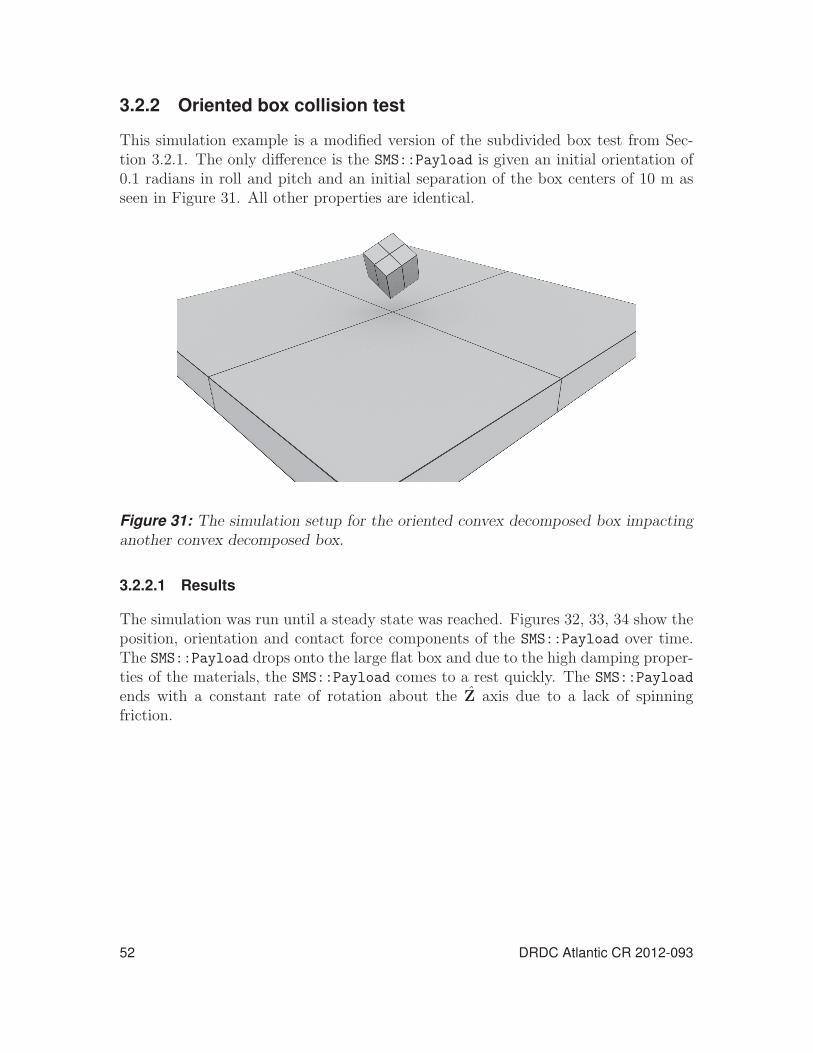
3.2.2 Oriented box collision test
This simulation example is a modified version of the subdivided box test from Sec-tion 3.2.1. The only difference is the SMS::Payload is given an initial orientation of0.1 radians in roll and pitch and an initial separation of the box centers of 10 m asseen in Figure 31. All other properties are identical.
Figure 31: The simulation setup for the oriented convex decomposed box impactinganother convex decomposed box.
3.2.2.1 Results
The simulation was run until a steady state was reached. Figures 32, 33, 34 show theposition, orientation and contact force components of the SMS::Payload over time.The SMS::Payload drops onto the large flat box and due to the high damping proper-ties of the materials, the SMS::Payload comes to a rest quickly. The SMS::Payload
ends with a constant rate of rotation about the Z axis due to a lack of spinningfriction.
52 DRDC Atlantic CR 2012-093

-2
0
2
4
6
8
0 0.5 1 1.5 2
Payload
Position(m
)
time (s)
XYZ
Figure 32: The simulated position for the pre-oriented convex decomposed SMS::-
Payloads over time.
-0.2
-0.15
-0.1
-0.05
0
0.05
0.1
0.15
0.2
0 0.5 1 1.5 2
Payload
Orientation
(rad
)
time (s)
XYZ
Figure 33: The simulated orientation for the pre-oriented convex decomposed SMS::-
Payloads over time.
DRDC Atlantic CR 2012-093 53

-400000
-200000
0
200000
400000
600000
800000
0 0.5 1 1.5 2
Con
tact
Force
(N)
time (s)
StiffnessDamping
Figure 34: The simulated stiffness and damping components of the pre-oriented con-vex decomposed SMS::Payloads over time.
3.2.2.2 A discussion on rolling resistance
It is important to note that convex decomposition of the box into four pieces has theadded benefit of distributing the volumes of interferences into four spatially spreadcontact volumes. When the box has an angular velocity, the individual volumes ofinterference will experience different rates of change, thus creating some rotationaldamping resistance. This effect helps to approximate the effect of rolling resistance.If the box consisted of single convex pieces, the relative angular velocity of the ob-jects would cause no change in the volume of interference and little energy would bedissipated as indicated in Figure 35 a) and b). The individual volumes of interferencefor the sub-pieces of a subdivided box for the same contact situation would howeversee volume rates of change and thus dissipate energy due to rolling resistance, seeFigure 35 c) and d). Rolling resistance has not yet been implemented in the SMSAPI and can only be approximated by decomposing the objects into sub-pieces.
To demonstrate this phenomena through simulation, the first 1.5 seconds of the sim-ulation presented in this section is reproduced with a one piece box, a 4 piece boxand a 16 piece box. The one piece box reacts significantly differently to the contactin Figure 36 than the 4 piece box, while the reactions of the 4 piece and 16 piecebox in Figure 37 are quite similar since they both handle rolling resistance similarly.An alternative to relying on many sub-pieces to model rolling resistance that may beinaccurate and increase computational demand is the inclusion of a rolling resistancemodel [20].
54 DRDC Atlantic CR 2012-093

F(V, dVdt)
cg cg
cg cg
a) b)
c) d)
F(V, dVdt)
F(V, dVdt)F(V, dVdt ) F(V, dV
dt)F(V, dV
dt)
ω
ω
Figure 35: A description of the effect of angular velocity, ω, on the contact forcewithout rolling resistance for a one-piece convex box and a subdivided box. Theinitial state of the a) one-piece and c) subdivided box, showing the contact forcecause by the individual volumes of interference, and the next time step showing nochange in the volume of interference for the one-piece box in b) and the changes inthe volumes of interference of the sub pieces of the convex decomposed box d).
DRDC Atlantic CR 2012-093 55

-2
0
2
4
6
8
0 0.5 1 1.5 2
Payload
Position(m
)
time (s)
1-Piece Box - X1-Piece Box - Y1-Piece Box - Z4-Piece Box - X4-Piece Box - Y4-Piece Box - Z
Figure 36: A comparison of the position of the 1 piece and 4 piece subdivided pre-oriented box SMS::Payloads over time.
-2
0
2
4
6
8
0 0.5 1 1.5 2
Payload
Position(m
)
time (s)
4-Piece Box - X4-Piece Box - Y4-Piece Box - Z16-Piece Box - X16-Piece Box - Y16-Piece Box - Z
Figure 37: A comparison of the position of the 4 piece and 16 piece subdivided pre-oriented box SMS::Payloads over time.
56 DRDC Atlantic CR 2012-093

3.2.3 Multiple contact point collision test
A scenario was created to test that the SMS::Payload can make contact with twoseparate external objects. The simulation consists of an SMS::Payload describedgeometrically with an elongated box with dimensions of 1m × 8.25m × 1m droppingonto two small 1 m × 0.9 m × 1.45 m boxes whose centers are separated by 6.75m as shown in Figure 38. The SMS::Payload has a mass of 40,000kg and the massmoments of Inertia about the X, Y, and Z axes are 3,333 kg·m2, 233,000 kg·m2,and 233,000 kg·m2, respectively. Both object material properties consist of a Young’smodulus of 20 GPa and a damping factor of 1 MPa·s. The SMS::Payload starts thesimulation with a small air gap between itself and the boxes which it will come torest on.
The collision detection system will detect two collisions, resolve two volumes of inter-ference, and apply two contact forces to the SMS::Payload. The system is consideredto be functioning properly if the SMS::Payload comes to rest on the two externalboxes.
Figure 38: The simulation setup of the multiple contact point simulation example.
3.2.3.1 Results
Figure 39 shows that the SMS::Payload comes in contact with external boxes anddue to the high damping of the material settles to a steady state rest. Figure 40 showsthat the SMS::Payload oscillates back and forth about the X axis until a balance isachieved as the contact forces imparts opposing moments. The contact force stiffnesscomponent shown in Figure 41 oscillates about 3.9e6 N to match the weight of theSMS::Payload, while the volume of interference in Figure 42 is negligible for theduration of the simulation due of the high stiffness of the material.
DRDC Atlantic CR 2012-093 57

-0.1
-0.05
0
0.05
0 1 2 3 4 5
Payload
Position(m
)
time (s)
XYZ
Figure 39: The position of the SMS::Payload over time.
-0.01
-0.005
0
0.005
0.01
0.015
0.02
0 1 2 3 4 5
Payload
Orientation
(rad
)
time (s)
XYZ
Figure 40: The Orientation of the SMS::Payload over time.
58 DRDC Atlantic CR 2012-093

-500000
0
500000
1e+006
1.5e+006
2e+006
0 1 2 3 4 5
Con
tact
Force
(N)
time (s)
StiffnessDamping
Figure 41: The contact force components of the SMS::Payload over time.
-0.005
0
0.005
0.01
0.015
0.02
0.025
0.03
0 1 2 3 4 5
Volume(m
3)or
Distance(m
)
time (s)
Total VolumeMSD/MTD
Figure 42: the volume of interference and MSD/MTD of the SMS::Payload overtime.
DRDC Atlantic CR 2012-093 59

3.2.4 Boat and cradle collision test
This simulation example demonstrates the ability of the SMS API to handle collisiondetection and contact dynamics of complex concave geometries with fine detail bydecomposing it into convex sub-pieces. The SMS::Payload for this test case is arescue boat. The hydrodynamics hull for the rescue boat was manually decomposedinto 19 convex sub-pieces as shown in Figure 43. These were passed through theQuickhull3D algorithm prior to being used in the collision detection system to ensuretheir convexity. A cradle was created using four convex boxes with one heavily taperededge that is used to support the boat as shown in Figure 44.
The material properties for the boat and cradle were both chosen to have a stiffness of100 MPa and a damping factor of 1.0 MPa·s. The boat is initially approximately halfa meter above its final resting position in the cradle. When the simulation begins, itfalls under gravity until it collides with the cradle and eventually comes to rest. Thesticking and sliding friction coefficients have both been set to 0.3.
3.2.4.1 Results
The boat begins from a height of 0.5 m and accelerates under gravity until it makescontact with the cradle as seen in Figure 45. When it makes first impact, it bouncesseveral times, but the kinetic energy of the boat is quickly dissipated through materialdamping. The boat makes first impact in the bow, which causes it to first pitch back.However, it quickly settles to its final resting state with a slightly negative pitch angleas seen in Figure 46. There was a maximum of 20 individual collision pairs duringthe collision which settled to 13 while at steady state as can be seen in Figure 47.
60 DRDC Atlantic CR 2012-093

Figure 43: The decomposition of the rescue boat hydrodynamic hull mesh into 19convex sub-pieces.
Figure 44: The boat and cradle simulation setup.
DRDC Atlantic CR 2012-093 61

-0.1
0
0.1
0.2
0.3
0.4
0.5
0 1 2 3 4 5
Payload
Position(m
)
time (s)
XYZ
Figure 45: The position of the SMS::Payload for the boat through time.
-0.05
-0.04
-0.03
-0.02
-0.01
0
0.01
0.02
0.03
0 1 2 3 4 5
Payload
Orientation
(rad
)
time (s)
XYZ
Figure 46: The orientation of the SMS::Payload for boat through time.
62 DRDC Atlantic CR 2012-093

0
5
10
15
20
0 1 2 3 4 5
Num.Con
tact
Points
time (s)
Figure 47: The number of collision pairs between the SMS::Payload and the cradlethrough time.
3.3 Generalised-α validationTwo tests were conducted to compared the performance of the Generalised-α integra-tor against the adaptive Runge-Kutta (RK45) integrator. The first test, presented insection 3.3.1, consists of the integration of a simple mass-spring-damper system. Thesecond test consists of the integration of a simple gravity pendulum system using acable, presented in section 3.3.2.
3.3.1 MSD
To verify the proper functioning of the Generalised-α integrator, a simple linear sys-tem was simulated and compared using both the Generalised-α and RK45 adaptiveintegrator. The simple linear system simulated here is a 1DOF mass-spring-damper.The simulation setup and results are described in Section 3.3.1.1 and Section 3.3.1.2,respectively.
3.3.1.1 Setup
The mass-spring-damper system, shown in Figure 48, consists of a mass of 1 kg, aspring with a spring constant of 1 N/m, and a damper damping factor of 0.4 Ns/m.This gives the system a natural frequency of 1 rad/s and a damping ratio of 0.2. Themass has an initial displacement from the static position of 5 m. When the simulationbegins, the free vibration of the mass is driven by the reaction forces imparted bythe spring and damper. Three Generalised-α simulations were run and comparedagainst a benchmark simulation that consists of the same system integrated with an
DRDC Atlantic CR 2012-093 63

RK45 integrator using a constant time step of 1e-3 s. The first simulation was givena spectral radius of 0 (maximum artificial dissipation) and a time step (dt) of 1e-3 s.The second simulation was given a spectral radius of 0 and a time step of 5e-1 s whilethe last simulation was given a spectral radius of 1 (no artificial dissipation) and atime step of 5e-1 s.
X
Figure 48: The setup for the Generalised-α mass-spring-damper test case.
3.3.1.2 Results
The simulation was executed for 50 seconds during which time the mass oscillateddue to its initial offset position. The underdamped vibrations were quickly eliminatedafter a few oscillations. The Generalised-α simulation with a time step of 1e-3 s andthe RK45 integrator simulation provided effectively identical results. However, theGeneralised-α simulation completed in 823 milliseconds while the RK45 simulationcompleted in 726 milliseconds. However, both integrators are constrained to integrateat the same constant rate and so this does not demonstrate the Generalized-α’s abilityto integrate at a larger time step than the RK45 integrator. Increasing the time stepsize in the generalised-α simulation while maintaining a spectral radius of 0 hadthe effect of increasing the amount of dissipation while the same simulation with aspectral radius of 1 results adhered much closer to the benchmark case.
3.3.2 Pendulum
Due to the nature of the Generalised-α integrator, the numerical dissipation providedshould only affect oscillations at periods smaller than the time step utilized and somore important lower frequency effects should not be significantly influenced. Fur-thermore, large, potentially unrealistic, structural damping values will not be neededto otherwise control these high frequency effects that could otherwise potentiallydestabilise the simulation as in the explicit integrator in certain circumstances. Thegravity pendulum test demonstrates how the Generalised-α integrator will accuratelysimulate the desired lower frequency behaviour in a complex stiff multiple DOF non-linear system. In this case, the lateral pendulum oscillation is low frequency, whichis unaffected, while the high frequency axial vibration induced from the cable initialconditions is damped.
64 DRDC Atlantic CR 2012-093

-4
-2
0
2
4
6
0 10 20 30 40 50
MassPosition(m
)
Time (s)
RK45 (dt = 1e-3s)Generalised-α (dt = 1e-3s, ρ = 0)Generalised-α (dt = 5e-1s, ρ = 1)Generalised-α (dt = 5e-1s, ρ = 0)
Figure 49: The time history of position of the mass for the mass spring damper usingthe Generalized-α integrator and the RK45 integrator.
3.3.2.1 Setup
The gravity pendulum system for this test, illustrated in Figure 50, consists of a 20m long vertical steel cable with a diameter of 5 mm. The cable has an axial stiffnessof 1.5e6 N. The cable has its top end fixed in space while the bottom end has aspherical mass of 5 kg attached. The cable is initially displaced by a small amountand is also given a small initial velocity to begin oscillation. The expected period ofoscillation from this system is 8.97 s. There is no damping in the system, such asair drag, other the axial material damping which had to be provided to the RK45simulation to maintain stability. The axial damping given to RK45 was 5 Ns whilefor the Generalised-α simulation the cable was given a material damping of 0.0 Ns.
Both the RK45 and Generalised-α simulations were run at a time step of 1.0e-4 s. TheGeneralised-α simulation was given a spectral radius of 0 to maximize the numericaldamping. The RK45 algorithm was locked at the desired time step by setting theminimum and maximum allowable time step to 1.0e-4 s.
3.3.2.2 Results
Both the RK45 and Generalised-α simulations completed successfully. The positionsof the mass at the end of the pendulum is plotted in Figure 51. The simulated periodof oscillation matches expectations for both integrators. However, the spectral radiusof 0 seems to have a damping effect on the low-frequency amplitude of oscillationof the pendulum, which was unexpected. Setting the spectral radius to 0.5 largelyremoves this low-frequency damping effect. Figures 52 and 53 show the tensions inthe cables for both integrators. Note the rapid damping out of the high frequency
DRDC Atlantic CR 2012-093 65

δX
Figure 50: The setup for the Generalised-α mass-spring-damper test case.
axial strain vibrations seen in tension time history in the Generalised-α simulationeven when there is no material damping used in the simulation.
The RK45 simulation has much larger material damping with a mild effect on the highfrequency axial strain vibrations. The execution times for both the Generalised-α andRK45 simulations were 148.478 s and 146.893 s, respectively. It is anticipated thatlarger time steps will be allowed by an adaptive Generalised-α integrator since thehigher frequency effects are damped out quickly and are a constraining factor on thestability of the simulation. An adaptive time step algorithm will likely significantlyimprove execution speed in the implicit numerical integrator in an analogous mannerto RK45’s performance benefits over RK4.
66 DRDC Atlantic CR 2012-093

-1
-0.5
0
0.5
1
0 20 40 60 80 100 120
Xposition(m
)
Time (s)
RK45GA
Figure 51: The X position of the mass over time for both the RK45 and Generalised-αintegrator simulations.
-600
-400
-200
0
200
400
600
0 20 40 60 80 100 120
Cab
leTension
inelem
ent1
(N)
time (s)
Figure 52: The cable tensions for the Generalised-α integrator simulation.
DRDC Atlantic CR 2012-093 67

-600
-400
-200
0
200
400
600
0 20 40 60 80 100 120
Cab
leTension
inelem
ent1
(N)
time (s)
Figure 53: The cable tensions for the RK45 integrator simulation.
68 DRDC Atlantic CR 2012-093

4 Launch and Recovery simulation
This section describes the process undertaken to produce the Launch and Recoverysimulation, in which a small craft is launched from a frigate, then recovered. Section4.1 describes the creation of a simplified version of the launch and recovery withoutcontact dynamics or naval frigate motions. The results of the simulation of the sim-plified version showed unacceptable simulation execution speeds. In order to executethe Launch and Recovery simulation at a reasonable rate, some time was spent tooptimise the code and to identify simulation bottlenecks. Section 4.2 describes theseefforts and their results. Finally, contact dynamics and naval frigate motions in waveswere added to the simulation to generate the final simulation. The simulation setupand results of the final simulation can be found in Section 4.3.
4.1 Simplified Launch and Recovery simulationA simplified simulation was first constructed to demonstrate the SMS API’s capabilityto simulate the launch and recovery of a small vessel from a naval frigate using aPalfinger-like boomcrane (Palfinger PK45000). The Simplified Launch and Recoverysimulation scenario is depicted in Figure 54. The simulation begins with the Palfinger-like crane attached to a naval frigate with an SMS::Cable attached to its last linkwhile the rescue boat is sitting still on the ship deck. Next, the boat is lifted off ofthe deck using the crane and winch. The boat is then placed in the water and thecable is detached from the boat. Next, the boat is reconnected with the cable andthen placed back on board the ship using the crane and winch.
This simulation demonstrates several key capabilities of the SMS API:
• Use of the Director class within the SMS API
• Boomcrane control
• Attachment and detachment of a cable to a payload midway through a simula-tion
• Winch operation
4.1.1 Simulation setup4.1.1.1 Boomcrane setup
The SMS::BoomCrane base is fixed in space to simulate being attached to the deckof a still ship. Its base frame relative to the Earth-fixed frame, P
(1)E→p is made of
3 Cartesian position components followed by 3 Euler angles which defines its orien-tation. The boomcrane’s first joint frame is defined in this simulation as P
(1)E→p =
DRDC Atlantic CR 2012-093 69

[ −1.0 0 18.5 0 0 0]. The Palfinger-like boomcrane begins the simulation ini-
tially in a folded state (see Figure 54), the initial D-H parameters for the SMS::-
BoomCrane are defined in Table 8. The details of the Palfinger-like boomcrane’srepresentative rigid body mass properties and CG locations can be found in [1].
Z = 18.5 m
Z = 10m
Z = 0 mZX
zboat
xboat
Figure 54: The simulation scenario for the Simplified Launch and Recovery sim-ulation. The Palfinger-like boomcrane is shown folded (dotted), with a zero jointconfiguration (solid) and in an unfolded pose (dashed).
4.1.1.2 Rescue boat setup (SMS::Payload)
The rescue boat is a 6 m long vessel provided to DSA by DRDC in the form ofa VRML geometry file, as shown in Figure 55 a). From this file, DSA generated aclosed mesh polyhedron representative hull which is used by the SMS API to calculatehydrodynamic loads. As in the towing simulation, the center of gravity of the rescueboat is located 0.04 m above the baseline and 1.7 m from the stern of the vessel. Therescue boat has a mass of 500 kg and mass moments of inertia about the X, Y and Zaxis of 400, 1541 and 1760 kg·m2 respectively. The cable connection point relative to
70 DRDC Atlantic CR 2012-093

Table 8: The SMS::BoomCrane’s initial D-H Parameters in a folded configuration forthe Simplified Launch and Recovery capabilities test. Entries with a ()∗ representthe joint variable.
Link id αi ai di θi1 90 -0.65 1.4 0∗
2 0 1 0 −15∗
3 90 0 0 −90∗
4 0 0 0∗ 05 0 0 0∗ 06 0 0 0∗ 07 0 0 0∗ 0
a) b)
Figure 55: The rescue boat a) visualization mesh and b) hydrodynamic polyhedralmesh.
the rescue boat’s body-fixed frame was set to PB→C = [0, 0, 1.5]T . The rescue boatbegins the simulation sitting on the deck of a ship at PE→B = [2.2, 0.0, 10.0]T . Forthis simplified simulation, contact dynamics has not been enabled.
4.1.1.3 Cable Setup
The SMS::Cable begins the simulation as 6 m long and hanging vertically with itsnode N attached to the CG of the SMS::BoomCrane’s last link. An SMS::Winch isattached to the cable’s node N . The cable element lengths are limited to no shorterthan 1m and no longer than 7 m. The SMS::Cable properties are set to EA = 1.0e7N, EI = 1.0e3 Nm2 and GJ = 1.0e3 Nm2. The cable has a density of steel and adiameter of 0.02 m.
4.1.1.4 Seaway Setup
DRDC Atlantic CR 2012-093 71

The ocean was assumed to be calm for this simplified simulation and no waves werepresent in the seaway.
4.1.1.5 SMS::Director script
// Place a hold on the payload’s position and orientation
// It’s lying on the Ship’s Deck
myDirector.AddCommand("testPayload hold X 2.2 holdX");
myDirector.AddCommand("testPayload hold Y 0.0 holdY");
myDirector.AddCommand("testPayload hold Z 10 holdZ");
myDirector.AddCommand("testPayload hold EX 0.0 holdEX");
myDirector.AddCommand("testPayload hold EY 0.0 holdEY");
myDirector.AddCommand("testPayload hold EZ 0.0 holdEZ");
// Fully Extend the BoomCrane
myDirector.AddCommand("testBoomCrane 1 0.7854 0.5");
myDirector.AddCommand("testBoomCrane 2 1.57 0.5");
myDirector.AddCommand("testBoomCrane 3 1.0 0.5");
myDirector.AddCommand("testBoomCrane 4 1.0 0.5");
myDirector.AddCommand("testBoomCrane 5 1.0 0.5");
myDirector.AddCommand("testBoomCrane 6 1.0 0.5");
//Pause for a second to let things settle a bit
myDirector.AddCommand("pause 1");
// Payout cable to pick up the payload
myDirector.AddCommand("testWinch testCable 12.4 1.5");
//Release the hold on the Payload and Soft Connect
//with the Cable
myDirector.AddCommand("testPayload release holdX");
myDirector.AddCommand("testPayload release holdY");
myDirector.AddCommand("testPayload release holdZ");
myDirector.AddCommand("testPayload release holdEX");
myDirector.AddCommand("testPayload release holdEY");
myDirector.AddCommand("testPayload release holdEZ");
myDirector.AddCommand("testPayload testCable connect
0.0 0.0 1.5 testWinch");
//Pause for a second to let things settle
myDirector.AddCommand("pause 1.0");
72 DRDC Atlantic CR 2012-093

// Payin cable and move the crane’s first joint by
// 90 degrees so the Payload is over the deck and
// over the water.
myDirector.AddCommand("testWinch testCable 8.0 1.0");
myDirector.AddCommand("testBoomCrane 0 1.57 0.5");
myDirector.AddCommand("pause 0.3");
// Payout cable lowering the boat into the water
myDirector.AddCommand("testWinch testCable 15 1.5");
myDirector.AddCommand("testWinch testCable 22.4 0.75");
//Disconnect the cable from the Payload
myDirector.AddCommand("testPayload testCable testWinch
disconnect 0.1");
//Play a hold on X, Y and EZ so the payload does not
//drift away too far.
myDirector.AddCommand("testPayload hold X -1.0 holdX");
myDirector.AddCommand("testPayload hold Y 3.3 holdY");
myDirector.AddCommand("testPayload hold EZ 0 holdEZ");
// Payin Cable in order to simulate a recovery.
myDirector.AddCommand("testWinch testCable 10.0 1.0");
// Wait a bit
myDirector.AddCommand("pause 2");
//Payout Cable in order to Recover the Payload
myDirector.AddCommand("testWinch testCable 22.4 1.5");
myDirector.AddCommand("pause 1");
//Release holds on the payload
myDirector.AddCommand("testPayload release holdX");
myDirector.AddCommand("testPayload release holdY");
myDirector.AddCommand("testPayload release holdEZ");
//Soft connect the cable to the payload
myDirector.AddCommand("testPayload testCable testWinch
connect 0 0.3 0.0 0.0 1.5");
DRDC Atlantic CR 2012-093 73

//Payin Cable and rotate back over the deck.
myDirector.AddCommand("testWinch testCable 10.0 1.0");
myDirector.AddCommand("testBoomCrane 0 0 0.5");
//Payout Cable and drop the Rescue boat on the deck
//of the ship.
myDirector.AddCommand("testWinch testCable 17.17 1.5");
myDirector.AddCommand("testPayload testCable testWinch
disconnect 0.1");
myDirector.AddCommand("testPayload hold X 2.2 holdX");
myDirector.AddCommand("testPayload hold Y 0.0 holdY");
myDirector.AddCommand("testPayload hold Z 5.0 holdZ");
myDirector.AddCommand("testPayload hold EX 0.0 holdEX");
myDirector.AddCommand("testPayload hold EY 0.0 holdEY");
myDirector.AddCommand("testPayload hold EZ 0.0 holdEZ");
//Payin Cable and fold the Palfinger completing
//the simulation
myDirector.AddCommand("testWinch testCable 6.0 1.0");
myDirector.AddCommand("testBoomCrane 6 1.0 0.5");
myDirector.AddCommand("testBoomCrane 5 1.0 0.5");
myDirector.AddCommand("testBoomCrane 4 1.0 0.5");
myDirector.AddCommand("testBoomCrane 3 1.0 0.5");
myDirector.AddCommand("testBoomCrane 2 1.57 0.5");
myDirector.AddCommand("testBoomCrane 1 0.7854 0.5");
4.1.2 Simulation results
The simulation performs as expected, The cable is connected to the payload at 23seconds. When the connection is made, the rescue boat’s 6 DOF hold is released.Next, the cable lifts up the boat, and drops it in the ocean and disconnects at 55seconds. The cable is reconnected at 95 seconds, lifted up and dropped back on theship deck, where the cable is then disconnected.
The boomcrane begins in a folded state and fully extends each joint sequentially.The unfolding process is completed at around 17 seconds. After the rescue boat isattached and lifted, the SMS::Boomcrane’s first joint is then actuated by π
4until the
boat is over the water. After the boat is recovered, the SMS::BoomCrane’s first joint isactuated back to its initial folded position. The first 18 seconds has the cable movingaround as the SMS::BoomCrane unfolds. The remainder of the simulation has the
74 DRDC Atlantic CR 2012-093

cable being payed in and out through the course of the simulation.
Plots of the simulation results for the various simulation components can be found inFigures C.1 through C.4. During the simulation, there were large tension oscillationsexperienced by the SMS::Cable while the payload was attached. This is likely causinga reduced integration time step in the adaptive integrator, and therefore slowingexecution speed during those phases of the simulation.
The simulation script shows that the SMS::BoomCrane should fold itself before thesimulation is completed. The actual simulation ended in a SMS::Cable destabilisationduring the last SMS::Payload disconnect procedure. It was first thought that thesoft disconnect time was set to 0.1 seconds which was likely not enough to reduce thetension in the cable. Thus when the cable was disconnected under tension, the cablereleased with too much stored elastic energy causing a snap load on release, potentiallycausing the destabilisation. However, later on, through further investigation it wasfound that a bug in the code was the culprit.
4.2 Improving execution speeds4.2.1 The integration timestep size
The adaptive Runge-Kutta (RK45) algorithm is the only integrator currently fullysupported by the SMS API. The algorithm adjusts the integration step size to mini-mize the error between 4th and 5th order approximation of the solution. In situationsof abrupt changes in state, the error can be high and thus the timestep size becomesreduced to minimize the error to below some tolerance. This self-adjusting mecha-nism of the RK45 integrator provides stability and efficient execution compared tofixed time step integrators.
Situations with large and abrupt accelerations tend to have smaller time steps. Mosttime-domain engineering simulations consist of objects with non-linear external dis-turbances acting on them and thus the integration timestep size is expected to varyover the course of a simulation as the system is perturbed.
When identifying areas of improvement in simulation scenario execution speeds, theintegration step size is an important indicator. For each order of magnitude thetime step size is reduced, an order of magnitude more dynamics calculations mustbe effectuated, which significantly decreases execution speed. On the other hand, anincrease in the time step size leads to immediate reductions in the number of dynamicscalculations required with much faster execution speed. Dynamics calculations for asingle time step can be expensive if for example a Payload with contact dynamics ormesh-based hydrodynamics functionality is enabled.
In systems where SMS::SimObjects are in a master-slave relationship, such as for an
DRDC Atlantic CR 2012-093 75

SMS::Cable attached to an SMS::Payload, the master SMS::SimObject’s integratorconcatenates the slave’s state vector to its own forcing the dynamics of both objectsto integrate at the same rate using the master’s integrator. If the SMS::Cable ismore prone to integration error than the SMS::Payload, it will negatively affectthe execution speed of the SMS::Payload since it will have to effectuate that manymore dynamics calculations. This problem is aggravated when the SMS::Payload’shydrodynamics feature is enabled, as those calculations tend to be costly. One way toavoid this phenomenon would be to simulate the SMS::SimObjects using their ownintegrators and their own step sizes. This functionality is not yet implemented in theSMS API. Prior to implementing independent integrators within the SMS API, eachSMS::SimObject’s code is being investigated independently.
To identify why the integration time step was falling so low in an earlier launch andrecovery simulation, the scenario was investigated in more detail. The results of theanalysis are presented in Section 4.2.1.1. Based on the analysis in Section 4.2.1.1, andto further identify or isolate the source of the low time steps, 4 variations of a caserepresentative of the operations that caused small timesteps of the launch and recov-ery simulation have been created. Section 4.2.1.2 discusses execution performance forthese tests in detail, optimizes the SMS::SimObject parameters to improve perfor-mance, and compares the before and after performance results of the 4 test variations.Finally, Section 4.2.2, the full launch and recovery simulation is re-run to check theperformance of the simulation with the optimized parameters.
4.2.1.1 The launch and recovery simulation
The launch and recovery simulation presented in Section 4.1 is representative of thetypes of operations and interactions the SMS API will be used for. A full script anddescription of the simulation can be found in Section 4.1. The operation, illustratedin Figure 56, consists of the following steps:
1. the crane unfolds
2. the cable pays out
3. the cable connects to the payload
4. the cable pays in
5. the crane rotates the payload overboard
6. the cable pays out
7. the cable disconnects from the payload, which floats in the water
8. the cable pays in
76 DRDC Atlantic CR 2012-093
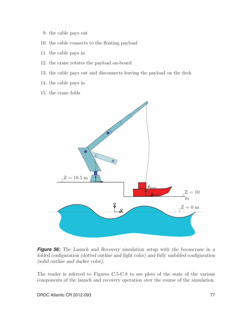
9. the cable pays out
10. the cable connects to the floating payload
11. the cable pays in
12. the crane rotates the payload on-board
13. the cable pays out and disconnects leaving the payload on the deck
14. the cable pays in
15. the crane folds
Z = 18.5 m
Z = 10m
Z = 0 mZX
zboat
xboat
Figure 56: The Launch and Recovery simulation setup with the boomcrane in afolded configuration (dotted outline and light color) and fully unfolded configuration(solid outline and darker color).
The reader is referred to Figures C.5-C.8 to see plots of the state of the variouscomponents of the launch and recovery operation over the course of the simulation.
DRDC Atlantic CR 2012-093 77

0
0.0001
0.0002
0.0003
0.0004
0.0005
0 50 100 150 200 250
IntegrationStepsize
(s)
Time (s)
Figure 57: The integration timestep size over the course of the Launch and Recoverysimulation.
Figure 57 shows the master SMS::SimObject’s (i.e. the SMS::Boomcrane’s) integra-tion time step variation through the course of the Launch and Recovery simulation.Small timesteps can be seen when the SMS::BoomCrane is actuating. Also the bestachievable time step with these properties appears limited to 4e-4.
This indicates poor time step sizes are caused by the PID joint controllers of theSMS::BoomCrane. Currently, the PID controllers achieve desired actuation solelywith proportional gain and viscous damping which results in a stiff system response.The SMS::Cable is also a possible limiting factor of time step sizes so it was alsoinvestigated as an avenue to improve the time step.
4.2.1.2 Identifying and resolving the source of small timesteps for arepresentative launch and recovery simulation.
Based on the analysis in Section 4.2.1.1 and to further help identify or isolate thesource of the small time steps, 4 variations of a case representative of the smalltimestep operations of the launch and recovery simulation were created. These testsconsist of the unfolded Palfinger-like boomcrane with an attached SMS::Cable thatin turn has an SMS::Payload attached at its other end. The first variation consistsof the SMS::Cable paying out by an SMS::Winch attached at the SMS::BoomCrane
end. The second variation has no SMS::BoomCrane with the SMS::Cable’s free nodefixed in space, the third variation is simply the SMS::BoomCrane, the SMS::Cable,and the SMS::Payload with no SMS::Winch, while the last variation is consists onlyof the SMS::Cable and SMS::Payload alone.
To see plots of the timestep size and the time ratios for the four setup variations
78 DRDC Atlantic CR 2012-093
over time the reader is referred to Figures C.9 and C.10 respectively. Large oscil-lation amplitudes in the time step of the simulation without the SMS::BoomCrane
are experienced and likely caused by small oscillations in the tension of the cableas the SMS::Winch begins to payout. Another cause is a slightly non steady stateinitial pre-tension in the cable from the SMS::Payload’s initial position. These os-cillations are not present when the SMS::BoomCrane is attached likely because theSMS::Boomcrane’s timestep is lower than the SMS::Cable’s.
The permutation with the SMS::Cable and SMS::Payload alone has a generally largetimestep of 3.5e-3 s, especially after the oscillations caused by non-equilibrium initialconditions are damped out. When an SMS::BoomCrane is involved, the simulationtime step is limited considerably to about 6.0e-4 s. The presence of an SMS::Winch
that is paying out cable also seems to be similarly limited. These findings indicate theSMS::BoomCrane PID controller coefficients must be better tuned to maximize thetime step and therefore simulation execution speed. This process and its results arepresented in Section 4.2.1.3. The SMS::Cable and SMS::Winch properties are thenadjusted to help improve simulation performance. This is described in Section 4.2.1.4.The 4 test variation cases presented here were executed again using these new tunedparameters and the results of which can be found in Section 4.2.1.4.
4.2.1.3 Tuning PID controllers and damping values
The SMS::Boomcrane induces a small timestep with potential for improvement asdiscussed in Section 4.2.1.2. It was postulated that the likely source of the smalltimestep was the PID controller gains. The PID controller was set up using only theP-control and some joint viscous damping was used to dampen out higher frequencyoscillation of the joints. To help increase the integration timestep sizes, the PIDcontroller P gains were reduced and the I-control gain was added to help achieve thedesired joint positions or velocities desired.
The original PID gains for the Palfinger-like boomcrane for the launch and recoverysimulation can be found in Table 9.
The PID gain tuning process consisted of tuning one joint at a time, starting withthe last joint and progressing sequentially towards the base. The tuning process usedhere is similar to the Ziegler-Nichols tuning process [21, 22]. To illustrate the tuningprocess, the second joint is used as an example. The boomcrane joint positions wereconfigured in such a way to reasonably load the joint by fully extending the crane andadding the payload to the attached cable. With the crane configured to appropriatelyload the joint, the following steps are followed to tune the PID controller gains toachieve a desired joint position of 45 degrees:
1. Reduce the viscous joint damping to ensure minimal influence during the tuningprocess.
DRDC Atlantic CR 2012-093 79
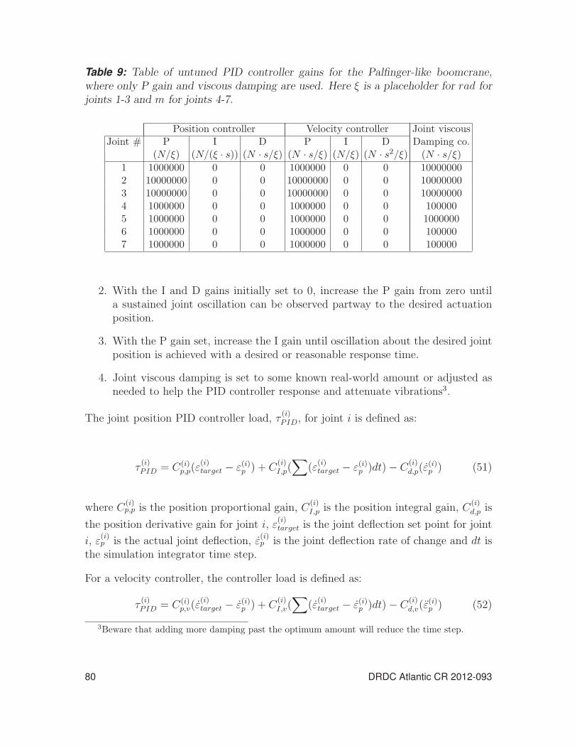
Table 9: Table of untuned PID controller gains for the Palfinger-like boomcrane,where only P gain and viscous damping are used. Here ξ is a placeholder for rad forjoints 1-3 and m for joints 4-7.
Position controller Velocity controller Joint viscousJoint # P I D P I D Damping co.
(N/ξ) (N/(ξ · s)) (N · s/ξ) (N · s/ξ) (N/ξ) (N · s2/ξ) (N · s/ξ)1 1000000 0 0 1000000 0 0 100000002 10000000 0 0 10000000 0 0 100000003 10000000 0 0 10000000 0 0 100000004 1000000 0 0 1000000 0 0 1000005 1000000 0 0 1000000 0 0 10000006 1000000 0 0 1000000 0 0 1000007 1000000 0 0 1000000 0 0 100000
2. With the I and D gains initially set to 0, increase the P gain from zero untila sustained joint oscillation can be observed partway to the desired actuationposition.
3. With the P gain set, increase the I gain until oscillation about the desired jointposition is achieved with a desired or reasonable response time.
4. Joint viscous damping is set to some known real-world amount or adjusted asneeded to help the PID controller response and attenuate vibrations3.
The joint position PID controller load, τ(i)PID, for joint i is defined as:
τ(i)PID = C(i)
p,p(ε(i)target − ε(i)p ) + C
(i)I,p(
∑(ε
(i)target − ε(i)p )dt)− C
(i)d,p(ε
(i)p ) (51)
where C(i)p,p is the position proportional gain, C
(i)I,p is the position integral gain, C
(i)d,p is
the position derivative gain for joint i, ε(i)target is the joint deflection set point for joint
i, ε(i)p is the actual joint deflection, ε
(i)p is the joint deflection rate of change and dt is
the simulation integrator time step.
For a velocity controller, the controller load is defined as:
τ(i)PID = C(i)
p,v(ε(i)target − ε(i)p ) + C
(i)I,v(
∑(ε
(i)target − ε(i)p )dt)− C
(i)d,v(ε
(i)p ) (52)
3Beware that adding more damping past the optimum amount will reduce the time step.
80 DRDC Atlantic CR 2012-093
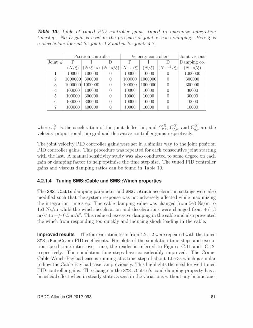
Table 10: Table of tuned PID controller gains, tuned to maximize integrationtimestep. No D gain is used in the presence of joint viscous damping. Here ξ isa placeholder for rad for joints 1-3 and m for joints 4-7.
Position controller Velocity controller Joint viscousJoint # P I D P I D Damping co.
(N/ξ) (N/ξ · s) (N · s/ξ) (N · s/ξ) (N/ξ) (N · s2/ξ) (N · s/ξ)1 10000 100000 0 10000 10000 0 10000002 1000000 300000 0 100000 1000000 0 3000003 1000000 1000000 0 100000 1000000 0 3000004 100000 100000 0 10000 10000 0 300005 100000 300000 0 10000 10000 0 300006 100000 300000 0 10000 10000 0 100007 100000 400000 0 10000 10000 0 10000
where ε(i)p is the acceleration of the joint deflection, and C
(i)p,v, C
(i)I,v, and C
(i)d,v are the
velocity proportional, integral and derivative controller gains respectively.
The joint velocity PID controller gains were set in a similar way to the joint positionPID controller gains. This procedure was repeated for each consecutive joint startingwith the last. A manual sensitivity study was also conducted to some degree on eachgain or damping factor to help optimise the time step size. The tuned PID controllergains and viscous damping ratios can be found in Table 10.
4.2.1.4 Tuning SMS::Cable and SMS::Winch properties
The SMS::Cable damping parameter and SMS::Winch acceleration settings were alsomodified such that the system response was not adversely affected while maximizingthe integration time step. The cable damping value was changed from 5e3 Ns/m to1e3 Ns/m while the winch acceleration and decelerations were changed from +/- 3m/s2 to +/- 0.5 m/s2. This reduced excessive damping in the cable and also preventedthe winch from responding too quickly and inducing shock loading in the cable.
Improved results The four variation tests from 4.2.1.2 were repeated with the tunedSMS::BoomCrane PID coefficients. For plots of the simulation time steps and execu-tion speed time ratios over time, the reader is referred to Figures C.11 and C.12,respectively. The simulation time steps have considerably improved. The Crane-Cable-Winch-Payload case is running at a time step of about 1.0e-3s which is similarto how the Cable-Payload case ran previously. This highlights the need for well-tunedPID controller gains. The change in the SMS::Cable’s axial damping property has abeneficial effect when in steady state as seen in the variations without any boomcrane.
DRDC Atlantic CR 2012-093 81

4.2.2 Improved launch and recovery simulation executionperformance
The improved SMS::SimObject properties obtained from Sections 4.2.1.3 and 4.2.1.4were used to rerun the Launch and Recovery simulation in order to compare theexecution performance. For plots of the simulation state of various simulation objectsover the course of the Launch and Recovery simulation with improved parameters,the reader is referred to Figures C.13 to C.16 respectively. The new PID controller,cable, and winch properties have affected the system’s response slightly, but moreimportantly it has increased integration time step considerably. The time steps arean order of magnitude larger in general as can be seen in Figure 58. This has favorablyaffected the simulation time ratio which is now 10:1 with the large majority of thesimulation running at 3:1.
0
0.002
0.004
0.006
0.008
0.01
0 50 100 150 200 250
IntegrationStepsize
(s)
Time (s)
Figure 58: The integration timestep size over the course of the improved launch andrecovery example simulation.
4.2.3 Profiling
To help determine how much time is spent in different parts of the code duringexecution, the code was instrumented and analysed using the AQTime code profilingsoftware. Doing this has allowed DSA to identify bottlenecks in execution speed. Toprofile the code, a representative simulation was required. The first second of theCrane-Cable-Winch-Payload test variation from Section 4.2.1.4 was selected. Thesetup was modified to help profile the hydrodynamics code as the SMS::Payload wasset to be initially floating on the water.
The code profile was obtained using AQTime and a copy of SMS API v0.1.261 andassociated code profiling test suite. The instrumented code profile can be found in
82 DRDC Atlantic CR 2012-093

Section 4.2.3.1. Based on the profile, the SMS API was updated to address some ofthe inefficiencies identified in the profile of SMS API v0.1.261. This updated code isversioned as SMS API v0.1.263 and its code profile can be found in Section 4.2.3.2.
Finally, the Launch and Recovery simulation was rerun using SMS API v0.1.263to compare against the results from Section 4.2.1.1. Those results can be found inSection 4.2.3.3.
4.2.3.1 Profile before improvements
The CalcDynamics() functions encapsulate most of the floating point operationscompleted by an SMS::SimObject during a simulation. The rest of the SMS APIcode is simulation management overhead. Though the the simulation managementcode merits profiling, it is not as critical to fast simulations as profiling of theCalcDynamics() function. Table 11 shows a list of the times with children for theCalcDynamics() functions of the SMS::SimObjects with hydrodynamics. Table 12updates the execution times for the SMS::Payload without hydrodynamics. Notethat the SMS::Winch::CalcDynamics() function is not included as the time spentexecuting that function was insignificant.
Table 11: The execution time of SMS API CalcDynamics() functions for 1.0 secondof simulation time with hydrodynamics calculations (SMS API v0.1.261).
Function Time with children (ms)
SMS::Payload::CalcDynamics() 9016.85
SMS::Boomcrane::CalcDynamics() 428.32
SMS::Cable::CalcDynamics() 165.00
Table 12: The execution time of SMS::Payload::CalcDynamics() andSMS::RigidBody::CalcDynamics() functions for 1.0 second of simulation timewithout hydrodynamics calculations (SMS API v0.1.261).
Function Time with children (ms)
SMS::Payload::CalcDynamics() 31.13
Each CalcDynamics() function in Table 11 and their related sub-functions were pro-filed line by line to identify if any line, function, or routine’s execution speeds couldbe improved. The SMS::BoomCrane::CalcDynamics() function profile and potentialsources for improvement are described in Section 4.2.3.1 with the SMS::Cable andthe SMS::Payload following in Sections 4.2.3.1 and 4.2.3.1, respectively.
DRDC Atlantic CR 2012-093 83

SMS::BoomCrane::CalcDynamics() The function CalcDynamics() was profiledon a line by line basis to identify the functions and operations that take the longestto execute. The majority of the issues identified as leading to poor performance forthis code are due to:
• the use of functions with vectorial (e.g. std::vector or UBLAS vector) returntypes,
• the use of function-scope temporary memory allocation and destruction, and
• the use of mutil::InvertMatrix() on orthogonal matrices when a much moreefficient transpose function would be ideally suited.
Table 13 lists the functions that took a significant amount of time to execute.
Table 13: The execution times of SMS::BoomCrane::CalcDynamics() sub-functionsfor 1.0 second of simulation time (SMS API v0.1.261).
% Time ofFunction BoomCrane::CalcDynamics() Time (ms)
ABA RigidBody:: 19.10% 81.89CalcForces()
ABA RigidBody:: 18.40% 78.81CalcInertiaRBFrame2JointFrame()
ABA RigidBody:: 17.29% 74.06CalcTransformationMatrices()
ABA RigidBody:: 11.38% 48.74CalcVelocities()
ABA RigidBody:: 4.05% 17.35GetNandBetaComponent()
To improve the SMS:BoomCrane’s performance, the problems identified above wereaddressed. The metric for improvement is the SMS::BoomCrane::CalcDynamics()
execution time and the execution times of the functions listed in Table 13.
SMS::Cable::CalcDynamics() The function Cable::CalcDynamics() was profiledon a line by line basis to identify the functions and operations that take the longestto execute. There were no major issues identified for potential improvement from theSMS::Cable class itself. That being said, the SMS::Cable class does call SMS::Rigid-Body and SMS::Winch functions if one is attached. These external class calls haveinefficient sections of code caused by:
• the use of functions with vectorial return types,
84 DRDC Atlantic CR 2012-093

• the use of function-scope temporary memory allocation and destruction, and
• the use of mutil::InvertMatrix() on orthogonal matrices when a much moreefficient transpose function would be ideally suited.
Table 14 lists the functions or lines of code that took the most time execute in theSMS::Cable::CalcDynamics() function.
Table 14: The execution times of SMS::Cable::CalcDynamics() sub-functions for1.0 second of simulation time (SMS API v0.1.261).
% Time ofFunction SMS::Cable::CalcDynamics() Time (ms)
SMS::Cable::CalcCableProfile() 35.13% 57.96
SMS::Cable::CalcExternalForces() 28.91% 47.70
SMS::Cable::CalcInternalForces() 19.97% 32.95
SMS::Cable::CurvatureAccel() 4.31% 7.11
SMS::Cable::CalcAccel() 3.87% 6.28
To improve the SMS::Cable’s performance, the problems identified above were re-solved. The metric for improvement was the SMS::Cable::CalcDynamics() execu-tion time and the execution times of the functions listed in Table 14.
SMS::Payload::CalcDynamics()
With hydrodynamics The functions Payload::CalcDynamics() and RigidBody-
::CalcDynamics() were profiled on a line by line basis to identify the functions andoperations that take the longest to execute. The majority of the issues identified asleading to poor performance for this code are due to:
• the use of functions with vectorial return types,
• the use of function level temporary memory allocation and destruction, and
• the use of mutil::InvertMatrix() on orthogonal matrices when a much moreefficient transpose function would be ideally suited.
Tables 15 through 17 list the functions that took the most time execute.
The hydrodynamic calculations require a considerable amount of effort because theforces must be computed individually for each one of the thousands of hydrodynamicmesh polygons. The hydrodynamic calculations were turned off to help highlightother inefficiencies in the SMS::Payload and SMS::RigidBody classes. To improve the
DRDC Atlantic CR 2012-093 85

Table 15: The execution times of SMS::Payload::CalcDynamics() sub-functionsfor 1.0 second of simulation time with hydrodynamics calculations enabled (SMSAPI v0.1.261).
% Time ofFunction SMS::Payload::CalcDynamics() Time (ms)
myRigidBody->CalcDynamics() 99.84% 9002.7
Table 16: The execution times of SMS::RigidBody::CalcDynamics() sub-functionsfor 1.0 second of simulation time with hydrodynamics enabled (SMS API v0.1.261).
% Time ofFunction SMS::RigidBody::CalcDynamics() Time (ms)
SMS::RigidBody::CalcForces() 99.83% 8987.4
Table 17: The execution times of SMS::RigidBody::CalcForces() sub-functions for1.0 second of simulation time with hydrodynamics enabled (SMS API v0.1.261).
% Time ofFunction RigidBody::CalcForces() Time (ms)
RigidBody::CalcHydroDynamicLoading() 53.33% 4793.0
RigidBody::CalcBuoyancy() 45.80% 4116.2
86 DRDC Atlantic CR 2012-093

SMS::RigidBody’s performance, the problems identified above were addressed. Themetric for improvement was the SMS::Payload::CalcDynamics() execution timeand the execution times of the functions listed in Tables 15 through 17.
Without hydrodynamics The SMS::Payload::CalcDynamics() and SMS::Rigid-
Body::CalcDynamics() functions were profiled on a line by line basis to identifythe functions and operations that take the longest to execute, this time without anyhydrodynamic force calculations. The majority of the issues identified as leading topoor performance for this function code are due to:
• the use of functions with vectorial return types,
• the use of function level temporary memory allocation and destruction, and
• the use of mutil::InvertMatrix() when a much more efficient transpose func-tion would be ideally suited.
Comparing Table 11 with Table 12 highlights how much time is spent calculatingthe hydrodynamic forces versus the rest of the SMS::Payload and SMS::RigidBody
dynamics calculations. This is due mostly because the hydrodynamics calculationsmust be repeated for each of the thousands of polygons that represent the rescueboat. Tables 18 through 20 lists the functions that took a significant amount oftime to execute without hydrodynamics involved.
To improve the SMS::Payload’s performance, the problems identified above will beresolved. The metric for improvement shall be the SMS::Payload::CalcDynamics()function execution time and the execution times of the functions listed in Tables 18through 20.
DRDC Atlantic CR 2012-093 87

Table 18: The execution times of SMS::Payload::CalcDynamics() sub-functions for1.0 second of simulation time without hydrodynamics (SMS API v0.1.261).
% Time ofFunction SMS::Payload::CalcDynamics() Time (ms)
myRigidBody->CalcDynamics() 69.87% 21.751
SMS::RigidBody::UpdateRBPosOri() 25.76% 7.7825
Table 19: The execution times of SMS::RigidBody::CalcDynamics() sub-functionsfor 1.0 second of simulation time without hydrodynamics (SMS API v0.1.261).
% Time ofFunction RigidBody::CalcDynamics() Time (ms)
RigidBody::CalcForces() 51.23% 11.143
RigidBody::CalcAccelerations() 28.75% 6.25
RigidBody::CalcTd() 19.55% 4.25
RigidBody::CalcT() 0.22% 0.05
Table 20: The execution times of SMS::RigidBody::CalcForces() sub-functions for1.0 second of simulation time without hydrodynamics (SMS API v0.1.261).
% Time ofFunction RigidBody::CalcForces() Time (ms)
RigidBody::CalcContactForces() 41.68% 4.64RigidBody::CalcHydroDynamicLoading() 17.98% 2.00
RigidBody::CalcGrav() 19.61% 2.18RigidBody::ConvertForces() 9.25% 1.03RigidBody::CalcBuoyancy() 6.51% 0.72
RigidBody::CalcCoriolisForce() 4.95% 0.55
88 DRDC Atlantic CR 2012-093

4.2.3.2 Profile after improvements
Areas of poor performance were identified using AQTime. The majority of the poorperformance was due to the use of functions with vector or matrix return types, theuse of in-function or worse in-loop vector or matrix memory allocations, and the useof matrix inversions of orthogonal matrices when the transpose would be faster to exe-cute. These issues have been addressed one by one and a new instrumented code pro-file of the same case discussed in Section 4.2.3.1 was regenerated. Table 21 shows a listof the times with children for the CalcDynamics() functions of the SMS::SimObjectswith hydrodynamics. Table 22 updates the execution time for the SMS::Payload
without hydrodynamics. Note that the SMS::Winch::CalcDynamics() function isnot included as the time spent executing that function was insignificant.
Table 21: The execution time of SMS API CalcDynamics() functions for 1.0 secondof simulation time, with hydrodynamics calculations (SMS API v0.1.263).
Function Time with Children (ms) Speed Up
SMS::Payload::CalcDynamics() 4762.43 1.89
SMS::Boomcrane::CalcDynamics() 177.63 2.41
SMS::Cable::CalcDynamics() 150.24 1.10
Table 22: The execution time of SMS::Payload::CalcDynamics() andSMS::RigidBody::CalcDynamics() functions for 1.0 second of simulation time,without a hydrodynamics (SMS API v0.1.263).
Function Time with Children (ms) Speed Up
SMS::Payload::CalcDynamics() 20.49 1.52
Each CalcDynamics() function in Table 21 and their related subfunctions wereprofiled line by line to compare against the profile of the SMS API v0.1.261 pre-sented earlier. The SMS::BoomCrane::CalcDynamics() function profile is presentedin Section 4.2.3.2, with the SMS::Cable, and the SMS::Payload following suit inSections 4.2.3.2 and 4.2.3.2 respectively.
SMS::BoomCrane::CalcDynamics() Profiling was performed for function Boom-
Crane::CalcDynamics(). Table 23 lists the functions that took a significant amountof time to execute.
SMS::Cable::CalcDynamics() Table 24 lists the functions or lines of code that tookthe most time to execute in the SMS::Cable::CalcDynamics() function.
DRDC Atlantic CR 2012-093 89

Table 23: The execution times of SMS::BoomCrane::CalcDynamics() subfunctionsfor 1.0 second of simulation time (SMS API v0.1.263).
% Time ofFunction BoomCrane::CalcDynamics() Time (ms) Speed Up
ABA RigidBody:: 15.34% 27.25 2.71CalcTransformationMatrices()
ABA RigidBody:: 14.14% 25.12 1.94CalcVelocities()
ABA RigidBody:: 12.94% 22.98 3.56CalcForces()
ABA RigidBody:: 7.10% 12.612 6.25CalcInertiaRBFrame2JointFrame()
ABA RigidBody:: 2.52% 4.47 3.88GetNandBetaComponent()
Table 24: The execution times of SMS::Cable::CalcDynamics() subfunctions for1.0 second of simulation time (SMS API v0.1.263).
% Time ofFunction Cable::CalcDynamics() Time (ms) Speed Up
Cable::CalcCableProfile() 35.31% 53.03 1.09
Cable::CalcExternalForces() 28.22% 42.39 1.12
Cable::CalcInternalForces() 19.37% 29.10 1.13
Cable::CurvatureAccel() 3.79% 5.69 1.25
Cable::CalcAccel() 5.14% 7.72 0.81
90 DRDC Atlantic CR 2012-093

SMS::Payload::CalcDynamics()
With hydrodynamics Tables 25 through 27 list the functions that took the mosttime execute.
Table 25: The execution times of the SMS::Payload::CalcDynamics() subfunctionsfor 1.0 second of simulation time with hydrodynamics enabled (SMS API v0.1.263).
% Time ofFunction Payload::CalcDynamics() Time (ms) Speed Up
myRigidBody->CalcDynamics() 99.88% 4755.68 1.89
Table 26: The execution times of SMS::RigidBody::CalcDynamics() subfunctionsfor 1.0 second of simulation time with hydrodynamics enabled (SMS API v0.1.263).
% Time ofFunction RigidBody::CalcDynamics() Time (ms) Speed Up
RigidBody::CalcForces() 99.82% 4747.10 1.89
Table 27: The execution times of SMS::RigidBody::CalcForces() subfunctions for1.0 second of simulation time with hydrodynamics enabled (SMS API v0.1.263).
% Time ofRigidBody::
Function CalcForces() Time (ms) Speed Up
RigidBody::CalcHydroDynamicLoading() 57.76% 2741.9 1.75
RigidBody::CalcBuoyancy() 41.54% 1971.9 2.09
Without hydrodynamics Comparing Table 21 with Table 22 highlights how muchtime is spent calculating the hydrodynamic forces versus the rest of the SMS::Payloadand SMS::RigidBody dynamics calculations. The hydrodynamics calculations stilldominate the execution times for the SMS::Payload due to the repetition of the hy-drodynamics calculations for each polygon. Tables 28 through 30 lists the functionsthat took a significant amount of time to execute without hydrodynamics involved.
DRDC Atlantic CR 2012-093 91

Table 28: The execution times of SMS::Payload::CalcDynamics() subfunctions for1.0 second of simulation time (SMS API v0.1.263).
% Time of Payload::Function CalcDynamics() Time (ms) Speed Up
myRigidBody->CalcDynamics() 81.86% 16.77 1.30
RigidBody::UpdateRBPosOri() 17.67% 3.62 2.15
Table 29: The execution times of SMS::RigidBody::CalcDynamics() subfunctionsfor 1.0 second of simulation time (SMS API v0.1.263).
% Time ofRigidBody::
Function CalcDynamics() Time (ms) Speed Up
RigidBody::CalcForces() 44.27% 7.42 1.5
RigidBody::CalcAccelerations() 37.71% 6.32 0.99
RigidBody::CalcTd() 17.39% 2.92 1.46
RigidBody::CalcT() 0.36% 0.06 0.83
Table 30: The execution times of SMS::RigidBody::CalcForces() subfunctions for1.0 second of simulation time (SMS API v0.1.263).
% Time ofRigidBody::
Function CalcForces() Time (ms)
RigidBody::CalcContactForces() 19.89% 1.47 3.16
RigidBody::CalcHydroDynamicLoading() 24.21% 1.97 1.01
RigidBody::CalcGrav() 15.84% 1.17 1.86
RigidBody::ConvertForces() 6.93% 0.51 2.02
RigidBody::CalcBuoyancy() 11.53% 0.85 0.85
RigidBody::CalcCoriolisForce() 8.62% 0.64 0.86
92 DRDC Atlantic CR 2012-093

4.2.3.3 Improvements to the launch and recovery simulation
After improvements to the SMS API code were made using a code profiling software,the Launch & Recovery simulation from Section 4.2.2 has be rerun to highlight theimprovements made in the SMS API v0.1.263 code. The 250 second simulationexecuted with a time ratio of 5.6:1 which is 1.7 times faster than the performancein Section 4.2.2 and 7.3 times faster than the original performance of the simulationfrom Section 4.2.1.1.
4.3 Full Launch and Recovery simulationAfter the Simplified Launch and Recovery simulation was profiled to improve execu-tion speed, it was expanded to include both ship motions as well as contact dynamics.To visualise the simulation results, a simple software tool was created. A screenshottaken from it can be seen in Figure 59. A geometric model of a Halifax class navalfrigate was obtained from DRDC and used to represent the ship in the seaway. Theship motions for this simulation were generated from ShipMo3D’s GenericFrigatesample project, which was modified slightly to suit this particular simulation sce-nario. The FreeMo module generated a time history of the position, velocity, andacceleration for the frigate which were then used to define the position of the base ofthe boomcrane as well as the position of the rescue boat cradle which is location onthe ship deck. The naval frigate has no forward velocity.
In the SMS simulation, the position, velocity, and acceleration of the frigate betweenwas linearly interpolated between time points obtained from ShipMo3D. These werethen used to extrapolate the position of the frigate over the course of simulation.
The boat and cradle simulation files from Section 3.2.4 were used in the Launch andRecovery simulation in that the rescue boat was given the same convex decomposedcontact geometry and the cradle was positioned and fixed on the ship deck. Thematerial properties of both the rescue boat and the cradle were maintained. Therescue boat was initially sitting in the cradle. The SMS API’s contact dynamicscapabilities prevent interference of the rescue boat and cradle, deck, and side of thenaval frigate.
A DeepSeaway::FixedRegularSeaway was used in SMS to model the seaway with 3m, 10 s waves, which were the same parameters used in ShipMo3D to generate theship’s motions. To help control the orientation of the rescue boat during the recoveryprocess and to guide it back into the cradle, a pair of cables were introduced intothe simulation to act as tag lines. Tension control winches were added to representhuman behavior in controlling the tag lines.
The full simulation script that governs this simulation is very similar to that found
DRDC Atlantic CR 2012-093 93

Figure 59: A screenshot from a visualisation of the Launch and Recovery simulation,showing the rescue boat, cradle, frigate, boomcrane, and cable.
in Section 4.1 with a few minor modifications. The boomcrane starts in a foldedconfiguration and the simulation process is as follows:
• the boomcrane unfolds,
• the lifting cable is attached to the rescue boat,
• the boat is lifted out of the cradle,
• the boat lowered into the water and detached from the cable.
From the water:
• the cable is reattached,
• the tag lines are attached to the boat,
• the boat is lifted back up,
• the boat lowered back into the cradle.
The full script can be found in the following section.
94 DRDC Atlantic CR 2012-093

4.3.0.4 Simulation script
#########################
#Unfold the crane
#########################
myCrane 1 0.7854 0.5
myCrane 2 1.57 0.5
myCrane 3 1.25 0.5
myCrane 4 1.25 0.5
myCrane 5 1.25 0.5
myCrane 6 1.25 0.5
myCrane 0 3.14 0.75
#######################################
#Payout the cable and attach the boat
############################
myWinch myCable 6.5 1.5
rescueboat myCable myWinch connect 0 0.5 0.0 0.0 1.5
pause 2
##################
#Lift the boat out of the cradle
###################
myWinch myCable 4 1.0
pause 2
#########################
#Rotate the crane overboard
##############
myCrane 0 1.57 0.5
####################
#Payout Cable
##################
myWinch myCable 15.5 1.5
#######################
#Disconnect the boat
##########################
rescueboat myCable myWinch disconnect 0.5
##########################################
#Payout a bit in preparation for reattachment
##################################
DRDC Atlantic CR 2012-093 95

myWinch myCable 17.5 3.5
pause 4
#####################
#Connect the boat
#####################
rescueboat myCable myWinch connect 0 0.5 0.0 0.0 1.5
#############
#Connect the taglines to the rescueboat
#######################
tagLineMan tagLine 15 1.0
tagLineManBack tagLineBack 15 1.0
rescueboat tagLine tagLineMan connect 0 3.0 3.0 0.0 0.4
tagLineMan tagLine 75
rescueboat tagLineBack tagLineManBack connect 0 3.0 -1.66 0.0 0.4
tagLineManBack tagLineBack 75
############
#Payin
########
pause 3
myWinch myCable 6 0.5
#######################
#Increase the tension
###########
tagLineMan tagLine 155
tagLineManBack tagLineBack 155
##########################
#complete the payin
###################
myWinch myCable 4 0.25
#############################
#Rotate over the cradle
#################
pause 2
myCrane 0 3.14 0.25
####################################################
#Payout the cable and disconnect the cable and tagline
96 DRDC Atlantic CR 2012-093

##################################
myWinch myCable 6.6 0.5
tagLineMan tagLine 30.0
tagLineManBack tagLineBack 30
pause 2
rescueboat tagLine tagLineMan disconnect 0.3
rescueboat tagLineBack tagLineManBack disconnect 0.3
pause 2
rescueboat myCable myWinch disconnect 0.3
######################
# Reel in a bit of cable
##################
myWinch myCable 4 0.25
######################
#Fold the crane, and Complete.
####################
myCrane 0 0 0.75
myCrane 6 0 0.5
myCrane 5 0 0.5
myCrane 4 0 0.5
myCrane 3 0 0.5
myCrane 2 -1.57 0.5
myCrane 1 -0.26 0.5
pause 5
4.3.1 Simulation results
The Launch and Recovery simulation began with the naval frigate floating in waveswith no forward velocity. The boomcrane can be seen in the process of unfolding inFigure 60. The cable was then payed out, attached to the rescue boat, and lifted outof its cradle as shown in Figure 61.
The boomcrane rotated the rescue boat overboard and lowered it in to the water asshown in Figure 62. While in the water, the cable was detached from the rescue boatand was left to float there for a few seconds before both the boomcrane lifting cableand the two tag lines were attached to begin the recovery process. The tag lines wereused to help control the rescue boat orientation. A snapshot of the rescue boat beinglifted back up out of the water with the tag lines attached can be seen in Figure 63.
DRDC Atlantic CR 2012-093 97
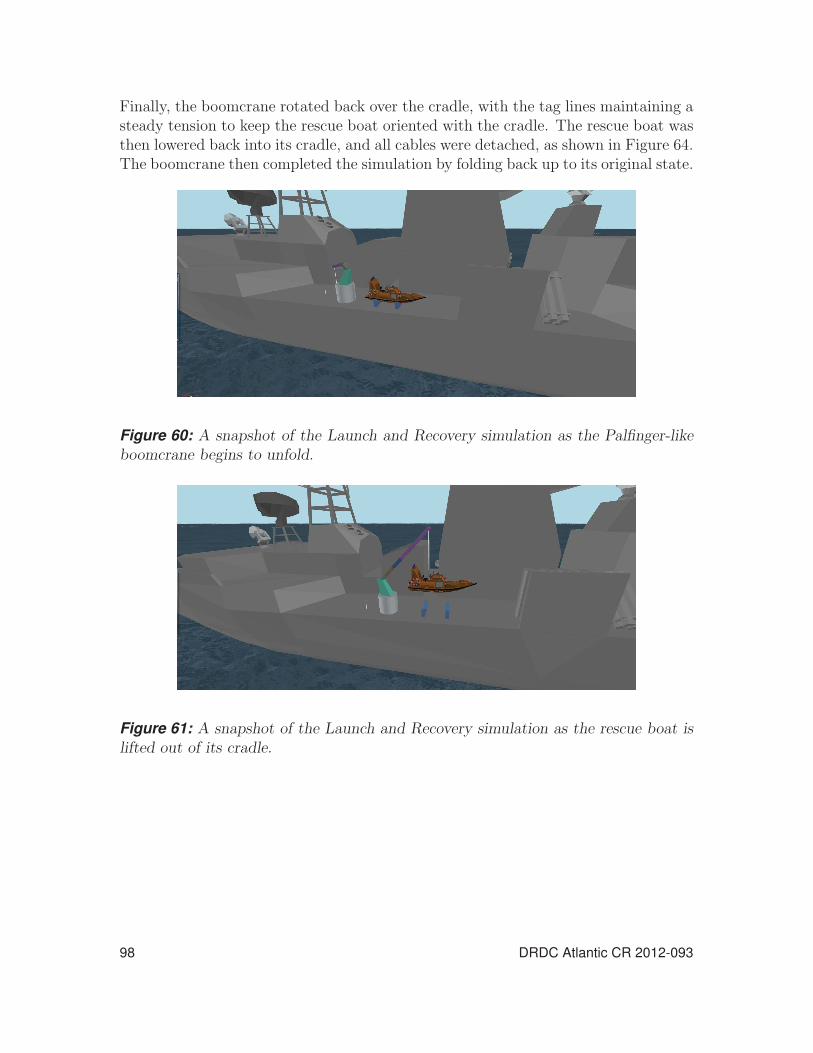
Finally, the boomcrane rotated back over the cradle, with the tag lines maintaining asteady tension to keep the rescue boat oriented with the cradle. The rescue boat wasthen lowered back into its cradle, and all cables were detached, as shown in Figure 64.The boomcrane then completed the simulation by folding back up to its original state.
Figure 60: A snapshot of the Launch and Recovery simulation as the Palfinger-likeboomcrane begins to unfold.
Figure 61: A snapshot of the Launch and Recovery simulation as the rescue boat islifted out of its cradle.
98 DRDC Atlantic CR 2012-093

Figure 62: A snapshot of the Launch and Recovery simulation after the rescue boatwas dropped in the water.
Figure 63: A snapshot of the Launch and Recovery simulation as the rescue boatis being lifted out of the water showing the tag lines used to prevent the boat fromyawing.
DRDC Atlantic CR 2012-093 99

Figure 64: A snapshot of the Launch and Recovery simulations with the rescue boatback in its cradle.
One of the challenges that arose when creating this scenario was that the simulationwas prone to destabilisation when the rescue boat is in the cradle. In this case, thenormal contact forces and friction forces between the cradle and the boat all sumup to act vertically against the rescue boat weight. Friction simulations, especiallyat low velocities around the stick-slip transition velocity, can be very stiff systemsand explicit integrators tend to have difficulty handling such stiff system [23]. Onepotential solution to resolving this issue may be the development of a more advancedfriction model that can mitigate difficulties at the transition velocity.
100 DRDC Atlantic CR 2012-093

5 Tuna Clipper Towing simulation
This section describes the creation of the Tuna Clipper Towing simulation. Section5.1 describes the creation of a simplified version of the towing simulation using therescue boat from the Launch and Recovery simulation and kinematically moving thefree end of the cable at a constant velocity. Section 5.2 describes the final TunaClipper Towing simulation which consists of a much larger vessel being towed in aseaway by a naval frigate whose motions were determined using ShipMo3D.
5.1 Simplified towing simulationA simplified simulation was designed to demonstrate the towing of a small vesselthrough a seaway. The simulation scenario is depicted in Figure 65 shows a smallvessel being towed by a cable. The cable is 20 m long and it is towing the small craftat a constant velocity through the seaway.
Vtow
Z = 0 mZX
zboatxboat
Figure 65: Simplified simulation of a small vessel tow.
5.1.1 Simulation Setup5.1.1.1 Payload setup
The 6m long rescue boat was provided to DSA by DRDC in the form of a VRMLgeometry file and can be seen in Figure 66 a). From this file, DSA generated a closedmesh polyhedron representative hull, as shown in Figure 66 b), which is used by theSMS API to calculate the hydrodynamic loading.
The actual mass properties of this vessel are unknown. For the purposes of testingthe SMS API, values were estimated for the key simulation parameters. The centerof gravity of the rescue boat was chosen to be located 0.04 m above the baselineand 1.7 m from the stern of the vessel. The rescue boat has a mass of 500 kg andmass moments of inertia about the X, Y and Z axis of 400, 1541 and 1760 kg·m2,respectively. The cable connection point relative to the rescue boat’s body-fixed framewas set to PB→C = [2.73, 0, 0.5]T . The rescue boat begins the simulation floating inthe wave at PE→B = [0.0, 0.0, 0.0]T .
DRDC Atlantic CR 2012-093 101

a) b)
Figure 66: The rescue boat a) visualization mesh and b) hydrodynamic polyhedralmesh.
5.1.1.2 Cable setup
The SMS::Cable towing the small vessel is 20 m long. It begins with its node 0attached to the small vessel and it is stretched out horizontally in the global Xdirection. The SMS::Cable’s node N is moved in the X direction at a velocity of1 m/s. The SMS::Cable’s properties are set to EA = 1.0e7 N, EI = 1000.0 Nm2
and GJ = 0.0 Nm2. The cable has a density of water and a diameter of 0.02. Nohydrodynamic forces are acting on the SMS::Cable.
5.1.1.3 Seaway setup
The seaway consists of a single regular wave oscillating with a period of 8 seconds,and an amplitude of 0.5 m. The wave has a heading of 90 degrees.
5.1.2 Simulation results
Figures 67 and 68 shows the boat position and the SMS::Cable’s node N, respectively.The boat is moving with a velocity of approximately 1 m/s. The accelerations of theboat is due to the elastic cable that stretches as it pulls the boat from an initialnon-moving state. The boat also heaves due to the ocean waves present.
5.2 Full Tuna Clipper Towing simulationThe final version of this simulation consists of an unpowered tuna clipper, a navalfrigate, and a towing line, as shown in Figure 69. In this simulation, the tuna clipperis modeled using an SMS::Payload object. A visualisation geometry of the tunaclipper was provided by DRDC from which a hydrodynamics mesh was generatedto provide hydrodynamics forces acting on the tuna clipper similarly to Figure 55.
102 DRDC Atlantic CR 2012-093

0
20
40
60
80
100
0 10 20 30 40 50
BoatPos
(m)
Time (s)
XYZ
Figure 67: The simulated rescue boat vessel position over time.
0
20
40
60
80
100
0 10 20 30 40 50
Cab
leNodeN
Pos
(m)
Time (s)
XYZ
Figure 68: The simulated cable node N position over time.
DRDC Atlantic CR 2012-093 103

The tuna clipper was provided drag coefficients of 1.5 and added mass coefficientsof 1.0 for all directions. Note that the tuna clipper is about 45 m in length, andthat the small body approximation (relative to the wave length) is assumed by theSMS::Payload’s hydrodynamics model. The simulation of the tuna clipper violatesthe small body approximation and thus the results may be inaccurate. However, thesimulation is intended as a proof of concept and the small body approximation allowsthis complex scenario to be simulated in a reasonable amount of time.
Figure 69: A visualisation of the Tuna Clipper Towing simulation.
The motions of the naval frigate were determined using DRDC’s ShipMo3D simula-tion software a-priori and used to kinematically control the end node of the cable.The naval frigate has a forward velocity of 2.5 m/s north and is floating in a seawaywith a 1.5 m wave height and 10 second period. The tuna clipper is 40 m long andwas given a mass of 400,000 kg. A 175 m tow cable is attached to the stern of thenaval frigate and the bow of the tuna clipper. The cable, assumed to be wire rope,has a diameter of 90 mm and an axial and bending stiffness of 5.0e8 N and 2.5e5 Nm2
respectively.
5.2.1 Results
A full animated visualization of the results of the simulation was submitted to DRDCwith this report. A screenshot of that visualisation can be found in Figure 69.
The tensions in the cable during the simulation are shown in Figure 70. The averagetension in the cable is approximately 60 kN.
104 DRDC Atlantic CR 2012-093

-500000
0
500000
1e+006
1.5e+006
2e+006
2.5e+006
0 10 20 30 40 50 60
Cab
leTension
inelem
ent4
(N)
time (s)
Figure 70: The tensions in the tow cable for the Tuna Clipper Towing simulation.
DRDC Atlantic CR 2012-093 105

6 Future work6.1 GeneralOne of the requirements of the SMS API is to provide the ability to conduct adistributed simulation by communicating the boundary conditions of various SMS::-SimObjects at regular intervals. While this capability has been implemented in abasic form, it should be expanded and properly tested.
Parallelizing of the hydrodynamics calculations could significantly improve the execu-tion speed of simulations. This could be supported either via GPGPU programmingor simple CPU multi-threading exploiting modern multi-core CPUs.
The SMS::Payload’s orientation is described and integrated over time using Eulerangles which have the potential to undergo a singularity event called “gymbal lock”.This is likely to occur and halt the simulation if the body passes through a 90-degree change in pitch. To alleviate the potential for such an event, quaternion basedorientation descriptions could be implemented as an option in the SMS API.
6.2 Winch classA relatively simple winch model that accounts for drum inertia and braking frictioncould be implemented to increase fidelity of the SMS::Winch class.
6.3 Contact dynamics6.3.1 Resolving N-body collisions
The current collision detection system does not scale well as it must effectuateO(NANB) collision checks where NA is the number of convex geometrical featuresthat make up the SMS::Payload and NB is the number of convex geometrical fea-tures that make up the external object. The system can only account for a singlerigid external object, such as the naval frigate, and so for example it cannot handlecollisions between an SMS::Payload and an SMS::BoomCrane. In order to providea scalable system to handle the ability to resolve the N-body collision problem, theimplementation of a broad-phase collision detection system would be required. Thefoundation for such a system has already been laid in the SMS API.
6.3.2 Continuous collision detection
The current SMS API contact resolution system only checks for instantaneous colli-sions and does not account for tunneling. Tunneling occurs when two objects passthrough each other in between time steps and will therefore not be detected without
106 DRDC Atlantic CR 2012-093

the use of continuous collision detection. To handle tunneling, continuous collisiondetection methods would be implemented, such as through the use of swept volumes.Tunneling is not an important phenomena to detect if the objects are large, andvelocities as well as time steps are small.
6.3.3 Rolling resistance implementation
Rolling resistance was discussed in Section 3.2.2.2 of this report. Rolling resistanceis currently not accounted for in the current contact model implementation, thougha crude effect is produced by hull partitioning.
6.3.4 Friction model improvements
An improved more continuous friction model could increase run times by reducinginstabilities that cause time-step reductions in the integrator. A potential candidatefor investigation could be the Gonthier et al. version of the LuGre friction model [24].In addition, spinning friction is currently not implemented. A simple Karnopp-stylefriction model is currently implemented. This model can have detrimental effects onthe integrator in high friction situations.
A more sophisticated friction model to help model lubricated conditions like wet shipdecks should also be implemented for increased accuracy. The LuGre friction modelwould account for this. Squeeze-film lubrication could also be taken into account andmight be important under some circumstances.
6.3.5 Volume of interference research
Computing the volume of interference is currently the execution speed bottleneckwhen a collision is occurring. Improvements in execution speed of simulations withcontact dynamics may require research into alternative methods of determining thevolume of interference. Computing the normal contact force direction using the MTDas well as the use of the volume of interference centroid as the contact point areapproximations that have some limitations.
6.3.6 Volume of interference limitations
The volume of interference algorithm implementation is limited to double precision.Errors can build up quickly after a few numerical operations in certain circumstances.A problem has been identified when the integration time step is small during the firstoccurrence of a collision. Volumes of interference smaller than 1e-9 m3 are generallynot detectable due to numerical precision and the algorithmic tolerances required tohandle such precision errors. This can lead to a very large instantaneous volume
DRDC Atlantic CR 2012-093 107

rate of change destabilizing the simulation. That is, the smallest detectable volumewill never be much smaller than 1e-9 m3 which will get divided by the time stepto obtain the volume rate of change. The time step can drop very low, while thevolume rate of change stays constant at the lowest discrete detectable level, leadingto unrealistically large damping factors. Currently, a workaround to this problemhas been implemented where the damping term is artificially limited to prevent thissituation from destabilizing the simulation. An alternative to this approach might beto use higher precision data types offered by, for example, the boost library, thoughthe use of such data types would come at the expense of execution speed. Logic couldpotentially be used to switch between regular doubles to higher precision data typeswhen situations requiring higher precision are encountered.
6.3.7 Winkler elastic bed depth
Computing the Winkler elastic bed depth is currently based on the radius of a spherewith the same volume of the sum of the convex sub pieces of the contact geometry.This is an approximation and more accurate methods of defining the elastic bed depthcould be identified.
6.3.8 Improving normal contact model fidelity
Currently the normal contact force model is modelled using a Winkler elastic beddepth where each spring is free to move independently of its neighbours. To im-prove the contact dynamics model, three dimensional contact stress effects, such asaccounting for Poisson’s ratio, for the contact model could be investigated.
6.4 Cable improvementsThere are several options for further development of the cable model.
6.4.1 Clamped terminations
The current cable model only supports pinned cable connections. Though clampedcable connection SMS::Payload and SMS::Boomcrane objects would only be neededin rare circumstances, particularly when flexural stiffness of the cable is high, it maybe desirable to implement that capability.
6.4.2 Implicit numerical integration
Promising results have been obtained with the implicit numerical integrator. In thesimple test cases studied so far, it successfully damps out high frequency effects.
108 DRDC Atlantic CR 2012-093

However, the simulation execution speed can likely be significantly increased by im-plementing an adaptive time step capability. This requires a method to assess errorin the simulation results as a function of time step. Generally, it is difficult to assesserror as computationally inexpensive as the RK45 algorithm does. However, a litera-ture review indicates that an error control algorithm is available for the Generalised-αmethod that affords significant increase in simulation execution speed and this shouldbe investigated. In addition, more insight is needed as to why validation experimentpendulum oscillations decay when such a small time step is utilized in conjunctionwith maximum numerical dissipation, which was unexpected.
The implicit integrator is currently only supported by the mass spring damper andcable models in isolation. Effort should be expended to facilitate using a separateintegrator for the cable when used in conjunction with the boomcrane and payloadmodels.
6.5 Launch and Recovery simulationThe Launch and Recovery simulation showed that the simple friction model usedby the contact force calculation model may induce numerical instability due to theabrupt transition between static and dynamic friction. One way to address this issuewould be to use a friction model that has a more continuous approach in modeling thetransition between static and dynamic friction and also includes a viscous component,as mentioned in the contact dynamics recommendations.
6.6 Tuna Clipper Towing simulationThe Tuna Clipper Towing simulation revealed the need for further software devel-opment to allow for environment load modeling for the cable due to the ShipMo3Dseaway. Additional development is needed to couple seaway effects with the cablehydrodynamics model.
DRDC Atlantic CR 2012-093 109

7 Conclusion
The preceding report reviews improvements to the SMS API, namely:
• the addition of a hydrodynamics model for the SMS::Payload class,
• the inclusion of the ShipMo3D::DeepSeaway class via DLL to model fluid envi-ronment,
• the creation of the SMS::Director class to facilitate the scripting of simulationevents,
• the general improvement of code performance by identifying and resolving bot-tlenecks,
• the improvement of the collision detection code by implementing a new collisiondetection software architecture, the EPA algorithm, and exploiting temporalcoherence,
• the investigation and implementation of the Generalised-α implicit integratorfor cables.
The new additions and improvements made to the SMS API have enabled the simu-lation of the launch and recovery of a small vessel in waves as well as the towing ofa small vessel through a seaway. These two simulations were set up, simulated, andvisualized. The visualizations were submitted to DRDC as attachments along withthis report.
110 DRDC Atlantic CR 2012-093

References
[1] Roy, A., Steinke, D., and Nicoll, R. (in review). Ship Mechanical Systems API– Final Report: Modeling Methodologies, API User Manual, API Validation.(DRDC Atlantic CR 2010-256). Defence Research and Development Canada –Atlantic.
[2] McTaggart, K.A. (2003). Modelling and Simulation of Seaways in Deep Waterfor Simulation of Ship Motions. (DRDC Atlantic TM 2003-190). DefenceResearch and Development Canada – Atlantic.
[3] Fish, P. R., Dean, R. B., and Heaf, N. J. (1980). Fluid-structure interaction inMorison’s equation for the design of offshore structures. Engineering Structures,2, 15–26.
[4] Det Norske Veritas (2007). Recommended practice DNV-RP-C205Environmental conditions and environmental loads.
[5] White, F. M. (1999). Fluid Mechanics, fourth ed. Toronto: McGraw-Hill.
[6] Dobrovolskis, A. R. (1996). Inertia of any polyhedron. Icarus, 124, 698–704.
[7] McTaggart, K.A. (2007). ShipMo3D Version 1.0 User Manual for SimulatingMotions of a Freely Maneuvering Ship in a Seaway. (DRDC Atlantic TM2007-172). Defence Research and Development Canada – Atlantic.
[8] McTaggart, K.A. (2002). Three Dimensional Ship Hydrodynamic CoefficientsUsing the Zero Forward Speed Green Function. (DRDC Atlantic TM2002-059). Defence Research and Development Canada – Atlantic.
[9] McTaggart, K.A. (2003). Hydrodynamic Forces and Motions in the TimeDomain for an Unappended Ship Hull. (DRDC Atlantic TM 2003-104).Defence Research and Development Canada – Atlantic.
[10] Sarpkaya, T. and Isaacson, M. (1981). Mechanics of Wave Forces on OffshoreStructures, Van Nostrand Reinhold.
[11] Garland, M. and Kirk, D. (2010). Understanding Throughput-OrientedArchitectures. Communications of the ACM, 53(11), 58–66.
[12] Muller, D. E. and Preparata, F. P. (1978). Finding the Intersection of TwoConvect Polyhedra. Theoretical Computer Science, Vol. 7, 2.
[13] van den Bergen, G. (2001). Proximity queries and penetration depthcomputation on 3D game objects. In Proc. Game Developers Conf.
DRDC Atlantic CR 2012-093 111

[14] Ericson, E. (2005). Real-Time Collision Detection, The Morgan KaufmannSeries in Interactive 3D Technology. Morgan Kaufmann Publishers.
[15] Gilbert, E. G., Johnson, D. W., and Keerthi, S. S. (1988). A Fast Procedure forComputing the Distance Between Complex Objects in three DimentionalSpace. IEEE Journal of Robotics and Automation, 4(2), 193–203.
[16] Chung, J. and Hulbert, G. M. (1993). A time integration algorithm forstructural dynamics with improved numerical dissipation: thegeneralized-alpha method. Journal of Applied Mechanics, 60, 371–375.
[17] Gobat, J. I. and Grosenbaugh, M. A. (2001). Applications of thegeneralized-alpha method to the time integration of the cable dynamicsequations. Computer methods in applied mechanics and engineering, 190,4817–4829.
[18] Low, Y.M. and Langley, R.S. (2006). Time and frequency domain coupledanalysis of deepwater floating production systems. Applied Ocean Research,28(6), 371–385.
[19] Chung, Jintai, Cho, Eun-Hyoung, and Choi, Keeyoung (2003). A priori errorestimator of the generalized-α method for structural dynamics. Int. J. Numer.Meth. Engng., 57(4), 537–554.
[20] Gonthier, Y., Mcphee, J., Lange, C., and Piedbœuf, J-C (2005). A ContactModeling Method Based on Volumetric Properties. Proceedings of IDETC’052005 ASME Design Engineering Technical Conferences and 5th InternationalConference on Multibody Systems, Nonlinear Dynamics and Control.
[21] Ziegler, J.G. and Nichols, N. B. (1942). Optimum settings for automaticcontrollers. Transactions of the ASME, 66, 759–768.
[22] Ogata, Katsuhiko (2002). Modern control engineering, 4 ed. Prentice-Hall, Inc.
[23] Gonthier, Y., McPhee, J., Lange, C., and Piedboeuf, J.-C. (2004). ARegularized Contact Model with Asymmetric Damping and Dwell-TimeDependent Friction. Multibody System Dynamics, 11, 209–233.
[24] Gonthier (2007). Contact Dynamics Modelling for Robotic Task Simulation.Ph.D. thesis. University of Waterloo.
112 DRDC Atlantic CR 2012-093

Annex A: Sample initialisation filesA.1 Cable class
//Verbose output mode on/off
$VERBOSE 1
/////////////////
//Cable material and geometrical properties
//Axial Stiffness
$EA 5e5
//Bending stiffness
$EI 20
//Torsional stiffness
$GJ 20
//Material density
$rho_cable 7778.0
//Axial damping
$CID 5e3
//Bending damping
$BCID 10
//ratio of compressive stiffness/tensile stiffness
$CE 1.0
//Cable Diameter
$dia_cable 0.02
/////////////
// Hydrodynamic properties
//Drag coefficient across cable
$CDc 1.0
//Added mass coefficient across cable
$CAc 1.0
/////////////////
// Element length control properties for Winch Payout/Payin
$ElementLengthMax 6
$ElementLengthMin 1
/////////////////////
// End-node boundary condition properties
DRDC Atlantic CR 2012-093 113

//end-nodes statically clamped in space, dynamics
//not computed for the end node if turned on.
$NODE0_STATIC 0
$NODEN_STATIC 0
//////////////////////
//Cable node initial conditions.
//Format: vX X vY y vZ Z
//Node 0
$0|IC 0 3.0426 0 8.4 0 6.4
//Node 1
$1|IC 0 3.0426 0 8.4 0 7.9
//Node 2
$2|IC 0 3.0426 0 8.4 0 9.4
//Node 3
$3|IC 0 3.0426 0 8.4 0 10.9
//Node 4
$4|IC 0 3.0426 0 8.4 0 12.4//
//Unstretched element lengths
$ElementLengths 1.525 1.525 1.525 1.527
//////////////////
// External spherical masses added to cable. Format:
//[0]: arcdistance to applied mass
//[1]: diameter of extmass
//[2]: density (dry) of extmass
//[3]: drag coefficient (optional, default: 1.0)
//[4]: added mass coefficient (optional, default: 0.5)
//external mass 0
$0|ExtMasses 0.1 0.1 7778 1.0 0.5
//external mass 1
$0|ExtMasses 0.1 0.1 7778 1.0 0.5
//Output folder for cable’s results files
//(relative or absolute path).
$OutputFolder LaunchAndRecovery/Results/Cable
114 DRDC Atlantic CR 2012-093

A.2 Winch class//The winch controller’s target velocity for
//velocity control mode
$VelocitySetPoint 0
//The winch controller’s target tension for
//tension control mode
$TensionSetPoint 15
//Forces the target velocity when in velocity
//control mode
$KinematicControl 1
//maximum positive acceleration
$accel_max 5
//maximum negative acceleration
$decel_max -25
//Winch controller’s PID coefficients
$Kp 0.01
$Kd 0.000001
$Ki 0.00001
//Output folder for Winch’s results files
//(relative or absolute path).
$OutputFolder LaunchAndRecovery/Results/Winch
A.3 Payload class//////////////////
// Payload Initial conditions (12 entries)
$0|IC 1 //Vx
$1|IC 0 //Vy
$2|IC 0 //Vz
$3|IC 0 //phiDot (Euler Z-Y’-X’’)
$4|IC 0 //thetaDot(Euler Z-Y’-X’’)
$5|IC 0 //psiDot (Euler Z-Y’-X’’)
$6|IC -1.35 //X
$7|IC 8.4 //Y
DRDC Atlantic CR 2012-093 115

$8|IC 9.6 //Z
$9|IC 0 //phi (Euler Z-Y’-X’’)
$10|IC 0 //theta (Euler Z-Y’-X’’)
$11|IC 3.14 //psi (Euler Z-Y’-X’’)
////////////////////////////////
// Mass Inertia Matrix about Body Frame
$0|Mass 500 0 0 0 0 0
$1|Mass 0 500 0 0 0 0
$2|Mass 0 0 500 0 0 0
$3|Mass 0 0 0 400 0 0
$4|Mass 0 0 0 0 1541 0
$5|Mass 0 0 0 0 0 1760
////////////////////
// Friction properties if using contact dynamics
//coulomb friction
$muc 0.05
//sticking friction
$mus 0.05
//Output folder for Payload’s results files
//(relative or absolute path).
$OutputFolder LaunchAndRecovery/Results/RescueBoat
A.4 Boomcrane class//Verbose output mode on/off
$VERBOSE 1
%%%%%%%%%%%%%%%%%%%%
%% Link 1 Red
%%%%%%%%%%
//Description of Link 1’s proximal joint frame relative
//to the base frame using Paul’s Denevit-Hartenberg
//parameter convention
//Format: alpha a d theta
$0|LinkDHParameters 90 -0.65 1.4 0
116 DRDC Atlantic CR 2012-093

//Defines whether the link’s proximal joint is revolute
//(’theta’) or prismatic (’d’)
$0|LinkJointVariable Theta
//target joint velocity when in velocity control mode.
$0|LinkJointVelocity 0
//The link’s rigidbody cg location relative to the proximal
//joint frame
$0|LinkCGLocation -0.35 0.0 0.7
//The link’s rigidbody body-fixed frame orientation relative to
//the proximal joint frame
$0|LinkCGOrientation 0 0 0
//The mass of the link’s rigidbody in the X Y and Z directions
$0|LinkMass 682.97 682.97 682.97
//The mass moment of inertia of the rigidbody described about the
//body-fixed frame(Ixx, Iyy, Izz)
$0|LinkMomentOfIntertia 139.44 139.44 55.776
//Joint controller’s control type (position or velocity)
$0|JointControlType position
//Joint controller’s position control PID gains
$0|JointProportionalCoefficientPos 10000
$0|JointIntegralCoefficientPos 100000
$0|JointDerivativeCoefficientPos 0
//Joint controller’s velocity control PID gains
$0|JointProportionalCoefficientVel 10000
$0|JointIntegralCoefficientVel 10000
$0|JointDerivativeCoefficientVel 0
//viscous damping coefficient for the joint
$0|JointViscousDamping 1000000
//The maximum allowable power applicable by the joint controller
$0|MaximumActuatablePower 10000000
//Joint limits to prevent the joint from actuating past some
DRDC Atlantic CR 2012-093 117

//threshold
$0|UpstreamJointLimits -1e30 1e30 //no limits
//Joint limit penalty force’s stiffness and damping coefficients
$0|JointLimitStiffness 10000
$0|JointLimitDamping 10000
%%%%%%%%%%%%%%%%%%%%
%% Link 2 Green
%%%%%%%%%%
$1|LinkDHParameters 0 1 0 -15
$1|LinkJointVariable Theta
$1|LinkJointVelocity 0
$1|LinkCGLocation 0.5 0 0
$1|LinkCGOrientation 0.0 0 0
$1|LinkMass 754 754 754
$1|LinkMomentOfIntertia 31.42 78.5 78.5
$1|JointControlType position
$1|JointProportionalCoefficientPos 1000000
$1|JointIntegralCoefficientPos 300000
$1|JointDerivativeCoefficientPos 0
$1|JointProportionalCoefficientVel 100000
$1|JointIntegralCoefficientVel 1000000
$1|JointDerivativeCoefficientVel 0
$1|JointViscousDamping 300000
$1|MaximumActuatablePower 10000000
$1|UpstreamJointLimits -45 90
$1|JointLimitStiffness 10000000
$1|JointLimitDamping 1000000
//Output folder for Winch’s results files
//(relative or absolute path).
118 DRDC Atlantic CR 2012-093

$OutputFolder LaunchAndRecovery/Results/Boomcrane
DRDC Atlantic CR 2012-093 119

This page intentionally left blank.
120 DRDC Atlantic CR 2012-093

Annex B: Descriptions of important classmethods
This section is a short, non-comprehensive manual to document some of the importantmethods that a user might require.
B.1 Payload class methodsB.1.1 Creating a payload object
An SMS::Payload object can be created using the class constructor:
SMS::Payload(std::string init file,
double t0,
bool file output)
where init file is a string that contains the location of the payload’s initializationfile, t0 is the start time of the cable object and file output is set to true to allowsimulation data to be output to disk.
B.1.2 Overridding the payload position and velocity
An SMS::Payload’s position and velocity can be overridden using:
SMS::Payload::SetPosOri(ub::vector<double> &posOri,
ub::vector<double> &posOriDot)
where posOri is a size 6 vector containing the Cartesian position followed by the 3Euler angles that describe its orientation, and posOriDot is the time rate of changeof posOri.
B.1.3 Overridding gravitational constant
An SMS::Payload’s gravitational constant can be overridden using:
SMS::Payload::SetGrav(double grav)
where grav is the new gravitational constant.
DRDC Atlantic CR 2012-093 121

B.2 Adding a hydrodynamics mesh for non-linearhydrodynamics
A hydrodynamics mesh can be provided to an SMS::Payload to allow for non-linearhydrodynamics forces to be calculated using:
SMS::Payload::InitialiseHydrodynamicPolyhedronWith3DS(
std::string file name,
double scaleX,
double scaleY,
double scaleZ,
ub::vector<double> &posOri,
ub::vector<double> &CDc,
ub::vector<double> &CAc)
where file name is the name of the .3ds geometry file, scaleX, scaleY and scaleZ
are the scaling factors for the geometry in the X, Y and Z directions respectively,posOri is the length 6 position and orientation vector, and CDc and CAc are length3 vectors that describe the drag and added mass coefficients in the X, Y and Zdirections respectively.
B.2.1 Defining wave conditions of the environment
Waves can be added to the SMS::Payload’s description of the enviroment usingShipMo3D’s DeepSeaway library. Currently, only fixed regular seaways are supported,adding it to the simulation can be accomplished using:
SMS::Payload::InitialiseEnvironmentAsFixedRegularSeaway(
std::string label,
double waterDensity,
double waveHeadingFromDeg,
double waveFreq,
double waveAmp,
double phaseDeg,
bool StokesSecondOrder,
bool WheelerStretching)
where label is the ocean label for identification purposes, waterDensity is thedensity of the water, waveHeadingFromDeg is the heading of the waves in degrees,waveFreq is the frequency of oscillation of the wave in radians, waveAmp is the am-plitude of the wave, phaseDeg is the phase of the wave in degrees, and StokesSe-
condOrder and WheelerStretching are flags that turn stokes second order wavesand Wheeler stretching on and off.
122 DRDC Atlantic CR 2012-093

B.2.2 Adding contact dynamics geometries
To enable contact dynamics between an SMS::Payload and the environment, geome-tries must be added to the SMS::Payload that describes the payload’s contact geom-etry as well the external object’s contact geometry. These can be done respectivelyusing:
SMS::Payload::Add3DSContactPolyhedron(
std::string file name,
double scaleX,
double scaleY,
double scaleZ,
ub::vector<double> &posOri)
SMS::Payload::AddExternal3DSContactPolyhedron(
std::string file name,
double scaleX,
double scaleY,
double scaleZ,
ub::vector<double> &posOri)
where file name is the name of the .3ds geometry file, scaleX, scaleY and scaleZ
are the scaling factors for the geometry in the X, Y and Z directions respectively, andposOri is the length 6 position and orientation vector. The position and orientationof the SMS::Payload’s contact objects are described relative to the SMS::Payload’sbody-fixed frame, while the position and orientation of the external object’s contactgeometriess are described relative to the external object’s origin which defaults to theinertial frame’s origin.
The geometries added must be convex. Multiple convex objects can be added to thePayload to build more complex concave shapes.
B.2.3 Setting the material properties for contact dynamics
The material properties for both the SMS::Payload’s and external object’s contactobjects can be set using:
SMS::Payload::SetMaterialProperties(double Young modulus set,
double B set)
SMS::Payload::SetExternalObjectMaterialProperties(
double Young modulus set,
double B set)
DRDC Atlantic CR 2012-093 123

where Young modulus set is the Young’s modulus and B set is the damping coeffi-cient.
B.2.4 Changing the position and orientation of the externalcontact objects
The position and orientation of the external contact objects are defined relative tothe external object’s origin. The origin of the external object can be redefined in theSMS::Payload using:
SMS::Payload::SetExternalContactPolyhedraPositionOrientation(
ub::vector<double> &posOri,
ub::vector<double> &posOriDot,
ub::vector<double> &posOriDotDot,
double &currTime)
where posOri is the length 6 position and orientation vector while posOriDot andposOriDotDot are the first and second time derivative of posOri.
B.2.5 Advancing simulation through time
SMS::Payload::AdvanceTime(double DeltaT)
B.2.6 Outputting simulation results to disk
SMS::Payload::OutputSimObjectData()
B.3 Cable class methodsB.3.1 Creating a Cable object
An SMS::Cable object can be created using the class constructor:
SMS::Cable(std::string init file,
double t0,
bool file output)
where init file is a string that contains the location of the cable’s initializationfile, t0 is the start time of the cable object and file output is set to true to allowsimulation data to be output to disk.
124 DRDC Atlantic CR 2012-093

B.3.2 Defining wave conditions of the environment
Waves can be added to the Cable’s description of the enviroment using ShipMo3D’sDeepSeaway library. Currently, only fixed regular seaways are supported, adding itto the simulation can be accomplished using:
SMS::Cable::InitialiseEnvironmentAsFixedRegularSeaway(
std::string label,
double waterDensity,
double waveHeadingFromDeg,
double waveFreq,
double waveAmp,
double phaseDeg,
bool StokesSecondOrder,
bool WheelerStretching)
where label is the ocean label for identification purposes, waterDensity is thedensity of the water, waveHeadingFromDeg is the heading of the waves in degrees,waveFreq is the frequency of oscillation of the wave in radians, waveAmp is the am-plitude of the wave, phaseDeg is the phase of the wave in degrees, and StokesSe-
condOrder and WheelerStretching are flags that turn stokes second order wavesand Wheeler stretching on and off.
B.3.3 Attaching a Winch to the cable
A SMS::Winch object can be added to an SMS::Cable to handle payin and payouteffects. The winch can be added to either the SMS::Cable’s node 0 or node N using:
SMS::Cable::AddWinch0(Winch &winch add)
SMS::Cable::AddWinchN(Winch &winch add)
respectively, where winch add is a reference to the winch object being attach.
B.3.4 Setting the Cable’s end node condition
The condition of the cable at its end nodes can be set using:
SMS::Cable::SetNode0BoundaryConditions(
ub::vector<double> &NodePos,
ub::vector<double> &NodeVel,
ub::vector<double> &NodeAccel)
DRDC Atlantic CR 2012-093 125

SMS::Cable::SetNode0BoundaryConditions(
ub::vector<double> &NodePos,
ub::vector<double> &NodeVel,
ub::vector<double> &NodeAccel)
for node 0 and N respectively where NodePos is the Cartesian position of the nodewhile NodeVel and NodeAccel are the first and second time derivatives of NodePos.
B.3.5 Advancing simulation through time
SMS::Cable::AdvanceTime(double DeltaT)
B.3.6 Outputting simulation results to disk
SMS::Cable::OutputSimObjectData()
B.4 Winch class methodsB.4.1 Creating a Winch object
An SMS::Winch object can be created using the class constructor:
SMS::Winch(std::string init file,
double t0,
bool file output)
where init file is a string that contains the location of the winch’s initializationfile, t0 is the start time of the winch object and file output is set to true to allowsimulation data to be output to disk.
B.4.2 Setting the winch’s controller mode
An SMS::Winch’s controller mode can be set to either velocity or tension control modeusing:
SMS::Winch::SetMode(std::string velocity or tension)
where velocity or tension is a string that can be set to either “velocity” for velocitycontrol or “tension” for tension control.
B.4.3 Setting the velocity control set point
The target velocity for velocity control mode can be set using:
126 DRDC Atlantic CR 2012-093

SMS::Winch::SetVelocitySetPoint(double setpoint)
where setpoint is the target velocity.
B.4.4 Setting the tension control set point
The target tension for tension control mode can be set using:
SMS::Winch::SetTensionSetPoint(double setpoint)
where setpoint is the target tension.
B.5 Boomcrane class methodsB.5.1 Creating a Boomcrane object
An SMS::Boomcrane object can be created using the class constructor:
SMS::Boomcrane(std::string init file,
double t0,
bool file output)
where init file is a string that contains the location of the boomcrane’s initializa-tion file, t0 is the start time of the boomcrane object and file output is set to trueto allow simulation data to be output to disk.
B.5.2 Attaching a Cable to one of the Boomcrane’s links
An SMS::Cable can be attached to a SMS::Boomcrane’s link using:
SMS::BoomCrane::AddCablePinned(int joint num,
SMS::Cable *cable to attach,
ub::vector<double> &location,
int end)
where joint num is the id of proximal joint belonging to the link the cable is beingattached to, cable to attach is a pointer to the cable being attached, location isa length 3 vector of the attachment location of the cable with respect to the link’sbody-fixed frame, and end is which end node of the cable is being attached: either 0for node 0 or 1 for node N.
B.5.3 Adjusting the boomcrane base position and orientation
The position of the SMS::Boomcrane’s base frame can be modified using:
DRDC Atlantic CR 2012-093 127

SMS::BoomCrane::SetBaseGlobalPositionAndOrientation(
ub::vector<double> &posOri,
ub::vector<double> &velocity,
ub::vector<double> &acceleration)
where posOri is a length 6 array containing the length 3 position of the base, andthe length 3 Euler angles, and posOriDot and posOriDotDot are its first and secondtime derivatives.
B.5.4 Advancing simulation through time
SMS::Cable::AdvanceTime(double DeltaT)
B.5.5 Outputting simulation results to disk
SMS::Cable::OutputSimObjectData()
B.6 Director class methodsB.6.1 Creation a Director object
A SMS::Director class object can be created to help control a simulation using:
SMS::Director()
B.6.2 Adding actors
SMS::SimObjects can be assigned to an SMS::Director to be controlled as an actorusing:
SMS::Director::AddActor(SimObject *object,
std::string actorName)
where object is a pointer to any of the child classes of SMS::SimObject, and actor-
Name is a label assigned to the actor for future identification.
B.6.3 Adding acting command to a script
A single command can be appended to a script using:
SMS::Director::AddCommand(std::string command)
where command is a string containing the command. A list of available commandscan be found in Section 2.2.
128 DRDC Atlantic CR 2012-093

B.6.4 Loading a script from file
A script can be loaded from file using:
SMS::Director::ReadScriptFromFile(std::string filePath)
where filePath is the absolute or relative path of the file to be loaded. A list ofavailable commands can be found in Section 2.2.
B.6.5 Managing a scene
Before every AdvanceTime call round, the Director must be told to manage the scene.The SMS::Director will check that commands are still in progress, or if completed,begin to the next command. This can be done using:
SMS::Director::ManageScene(double time,
double tStep)
where time is the current time of the scene and tStep is the time step for the nextAdvanceTime call.
DRDC Atlantic CR 2012-093 129

This page intentionally left blank.
130 DRDC Atlantic CR 2012-093

Annex C: Supplementary plotsC.1 Plots of the simplified Launch and Recovery
simulation from Section 4.1
-5
0
5
10
15
20
25
0 20 40 60 80 100 120 140
BoatPos
(m)
Time (s)
Boat X PositionBoat Y PositionBoat Z Position
Figure C.1: The simulated position of the rescue boat for the Simplified Launch andRecovery simulation (the X position indicated in red, the Y position indicated ingreen and the Z position indicated in blue).
DRDC Atlantic CR 2012-093 131
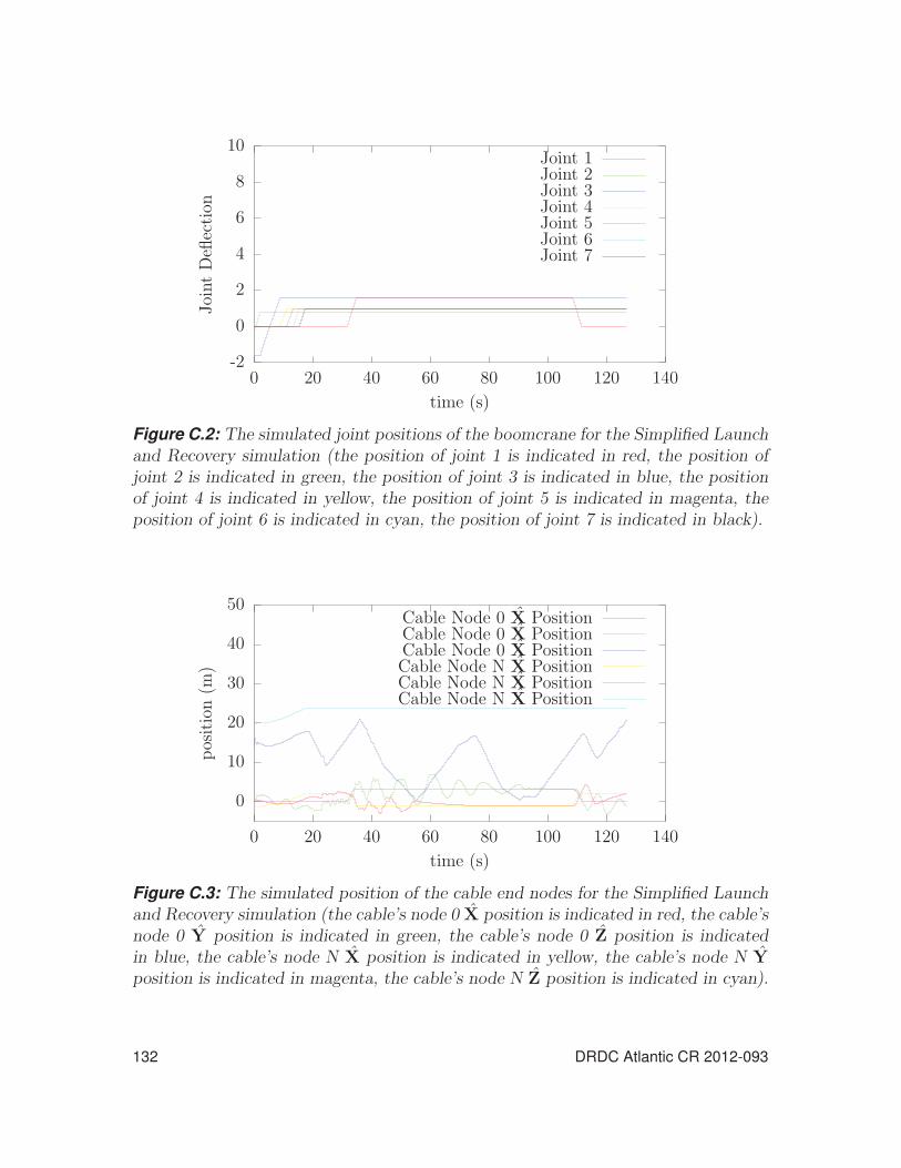
-2
0
2
4
6
8
10
0 20 40 60 80 100 120 140
JointDeflection
time (s)
Joint 1Joint 2Joint 3Joint 4Joint 5Joint 6Joint 7
Figure C.2: The simulated joint positions of the boomcrane for the Simplified Launchand Recovery simulation (the position of joint 1 is indicated in red, the position ofjoint 2 is indicated in green, the position of joint 3 is indicated in blue, the positionof joint 4 is indicated in yellow, the position of joint 5 is indicated in magenta, theposition of joint 6 is indicated in cyan, the position of joint 7 is indicated in black).
0
10
20
30
40
50
0 20 40 60 80 100 120 140
position(m
)
time (s)
Cable Node 0 X PositionCable Node 0 X PositionCable Node 0 X PositionCable Node N X PositionCable Node N X PositionCable Node N X Position
Figure C.3: The simulated position of the cable end nodes for the Simplified Launchand Recovery simulation (the cable’s node 0 X position is indicated in red, the cable’snode 0 Y position is indicated in green, the cable’s node 0 Z position is indicatedin blue, the cable’s node N X position is indicated in yellow, the cable’s node N Yposition is indicated in magenta, the cable’s node N Z position is indicated in cyan).
132 DRDC Atlantic CR 2012-093

0
10000
20000
30000
40000
50000
60000
70000
0 20 40 60 80 100 120 140
Tension
inBoatElement(0)
Time (s)
Figure C.4: The simulated tension of the cable’s first element for the SimplifiedLaunch and Recovery simulation.
C.2 Plots from the process of improving executionspeeds of the Launch and Recovery simulationfrom Section 4.2.1
-5
0
5
10
15
20
25
0 50 100 150 200 250
Payload
Position(m
)
time (s)
XYZ
Figure C.5: The position of the rescue boat over the course of the Launch and Re-covery simulation (the X position indicated in red, the Y position indicated in greenand the Z position indicated in blue).
.
DRDC Atlantic CR 2012-093 133

-2
-1
0
1
2
3
4
5
6
0 50 100 150 200 250
JointDeflection
s
time (s)
Joint1Joint2Joint3Joint4Joint5Joint6Joint7
Figure C.6: The position of the Palfinger-like boomcrane joints over the course ofthe Launch and Recovery simulation (the position of joint 1 is indicated in red, theposition of joint 2 is indicated in green, the position of joint 3 is indicated in blue,the position of joint 4 is indicated in yellow, the position of joint 5 is indicated inmagenta, the position of joint 6 is indicated in cyan, the position of joint 7 is indicatedin black).
-5
0
5
10
15
20
25
0 50 100 150 200 250
Positionof
Node0
(m/s)
time (s)
XYZ
Figure C.7: The position of the cable’s end node 0 over the course of the Launch andRecovery simulation (the cable’s node 0 X position is indicated in red, the cable’snode 0 Y position is indicated in green, the cable’s node 0 Z position is indicatedin blue, the cable’s node N X position is indicated in yellow, the cable’s node N Yposition is indicated in magenta, the cable’s node N Z position is indicated in cyan).
134 DRDC Atlantic CR 2012-093

0
20000
40000
60000
80000
100000
0 50 100 150 200 250
Cab
leTension
inelem
ent1
(N)
time (s)
Figure C.8: The tension in the cable’s first element over the course of the Launchand Recovery simulation.
C.3 Plots from the process of Identifying source ofsmall timesteps from Section 4.2.1.2
1.0e− 004
1.0e− 003
1.0e− 002
0 2 4 6 8 10
IntegrationStepsize
(s)
Time (s)
Crane, Winch, Cable, PayloadWinch, Cable, PayloadCrane, Cable, Payload
Cable, Payload
Figure C.9: The integration timestep size over the course of the simulation for the4 setup variations (Crane-Winch-Cable-Payload case indicated in red, Winch-Cable-Payload case indicated in green, Crane-Cable-Payload case indicated in blue, Cable-Payload case indicated in magenta).
DRDC Atlantic CR 2012-093 135

1.0e− 001
1.0e+ 001
1.0e+ 003
0 2 4 6 8 10
RealTim
e/Sim
Tim
eratio
Sim Time (s)
Crane, Winch, Cable, PayloadWinch, Cable, PayloadCrane, Cable, Payload
Cable, Payload
Figure C.10: The integration execution speed time ratio over the course of the simu-lation for the 4 setup variations (Crane-Winch-Cable-Payload case indicated in red,Winch-Cable-Payload case indicated in green, Crane-Cable-Payload case indicated inblue, Cable-Payload case indicated in magenta).
1.0e− 004
1.0e− 002
1.0e+ 000
0 2 4 6 8 10
IntegrationStepsize
(s)
Time (s)
Crane, Winch, Cable, PayloadWinch, Cable, PayloadCrane, Cable, Payload
Cable, Payload
Figure C.11: The integration timestep size over the course of the simulation forthe 3 setup variations (Crane-Winch-Cable-Payload case indicated in red, Winch-Cable-Payload case indicated in green, Crane-Cable-Payload case indicated in blue,Cable-Payload case indicated in magenta).
136 DRDC Atlantic CR 2012-093

1.0e− 001
1.0e+ 001
1.0e+ 003
0 2 4 6 8 10
RealTim
e/Sim
Tim
eratio
Sim Time (s)
Crane, Winch, Cable, PayloadWinch, Cable, PayloadCrane, Cable, Payload
Cable, Payload
Figure C.12: The time ratio over the course of the simulation for the 3 setup varia-tions (Crane-Winch-Cable-Payload case indicated in red, Winch-Cable-Payload caseindicated in green, Crane-Cable-Payload case indicated in blue, Cable-Payload caseindicated in magenta).
C.3.1 Plots of the optimised Launch and Recovery simulation ofSection 4.2.2
-5
0
5
10
15
0 50 100 150 200 250
Payload
Position(m
)
time (s)
XYZ
Figure C.13: The position of the rescue boat over the course of the improved launchand recovery example simulation (the X position indicated in red, the Y positionindicated in green and the Z position indicated in blue).
.
DRDC Atlantic CR 2012-093 137

-2
-1
0
1
2
3
4
0 50 100 150 200 250
JointDeflection
s
time (s)
Joint1Joint2Joint3Joint4Joint5Joint6Joint7
Figure C.14: The position of the boomcrane joints over the course of the improvedlaunch and recovery example simulation (the position of joint 1 is indicated in red,the position of joint 2 is indicated in green, the position of joint 3 is indicated inblue, the position of joint 4 is indicated in yellow, the position of joint 5 is indicatedin magenta, the position of joint 6 is indicated in cyan, the position of joint 7 isindicated in black).
-5
0
5
10
15
20
0 50 100 150 200 250
Positionof
Node0
(m/s)
time (s)
XYZ
Figure C.15: The position of the cable’s end node 0 over the course of the improvedlaunch and recovery example simulation (the cable’s node 0 X position is indicated inred, the cable’s node 0 Y position is indicated in green, the cable’s node 0 Z positionis indicated in blue, the cable’s node N X position is indicated in yellow, the cable’snode N Y position is indicated in magenta, the cable’s node N Z position is indicatedin cyan).
138 DRDC Atlantic CR 2012-093

0
5000
10000
15000
20000
0 50 100 150 200 250
Cab
leTension
inelem
ent1
(N)
time (s)
Figure C.16: The tension in the cable’s first element over the course of the improvedlaunch and recovery example simulation.
DRDC Atlantic CR 2012-093 139

This page intentionally left blank.
140 DRDC Atlantic CR 2012-093

DRDC Atlantic CR 2012-093 141
Distribution List
Improved Simulation of Ship Mechanical Systems
Andre Roy, Dean Steinke and Ryan Nicoll; DRDC Atlantic CR 2012-093; Defence R&D Canada – Atlantic; May 2012.
LIST PART 1: Internal Distribution by Centre
1 Author (1 hard copy)
3 DRDC Atlantic Library (1 hard copy)
3 Project Officer ABCA-09-0001 (H/WP) for distribution
4 Project Officer ABCANZ-97-12 (H/WP) for distribution
11 TOTAL LIST PART 1 (9 CDs, 2 Hard Copies) LIST PART 2: External Distribution by DRDKIM
1 Library and Archives Canada
Attn: Military Archivist, Government Records Branch
1
DRDKIM 3
1 DMSS 2 555 Blvd. De la Carriere Gatineau, QC K1A 0K2
1 Canadian Forces Maritime Warfare School Attention: Commanding Officer PO Box 99000 STN Forces Halifax, NS B3K 5X5
1 Director General Institute for Ocean Technology National Research Council of Canada P.O. Box 12093, Station A St. John's, NL A1B 3T5

142 DRDC Atlantic CR 2012-093
1 Transport Canada / Marine Safety Tower C, Place de Ville 330 Sparks Street, 11th Floor Ottawa, ON K1A ON8
2 Commanding Officer (2 hard copies) U.S. Coast Guard Research and Development Center 1082 Shennecosett Road Groton, CT 06340-2602
1 Ministry of Defence Attn: Head, Naval Research Dept. of Naval Architecture and Marine Engineering and Development P.O. Box 20702 2500 ES, The Hague The Netherlands
1 FOI Swedish Defence Research Agency Attn: Eva Dalberg Grindsjon Research Centre SE-147 25 Tumba Sweden
1 Department of Defence (Navy Office) Attn: Director Naval Ship Design Campbell Park Office CPI-505 Canberra ACT 2600 Australia
1 Document Exchange Centre Defence Information Services Branch Department of Defence Campbell Park Offices CP2-5-08 Canberra ACT 2600 Australia
1 Bundesamt fur Wehrtechnik und Beschaffung - SG I 3 Postfach 7360 6057 Koblenz Germany

DRDC Atlantic CR 2012-093 143
1 Dr. John Duncan Head of Simulation Based Acquisition Defence Equipment and Support Abbey Wood Mail Point 8014 BRISTOL BS34 8JH UK
1 Michael Dervin PMO Canadian Surface Combatant DGMPD(L&S) NDHQ 101 Colonel By Drive Ottawa, ON K1A 0K2
1 Frank Patsula PMO AOPS DGMPD(L&S) NDHQ – 101 Colonel By Drive Ottawa, ON K1A 0K2
1 Ken Holt PMO JSS DGMPD(L&S) NDHQ 101 Colonel By Drive Ottawa, ON K1A 0K2
1 Mr. M. Tunnicliffe DSTM 7 NDHQ 101 Colonel By Dr. Ottawa, ON K1A 4516
18 29
TOTAL LIST PART 2 (16 CDs, 2 HARD COPIES) TOTAL COPIES REQUIRED (25 CDs, 4 HARD COPIES)

144 DRDC Atlantic CR 2012-093
This page intentionally left blank.

DOCUMENT CONTROL DATA(Security markings for the title, abstract and indexing annotation must be entered when the document is Classified or Designated.)
1. ORIGINATOR (The name and address of the organization preparing thedocument. Organizations for whom the document was prepared, e.g. Centresponsoring a contractor’s report, or tasking agency, are entered in section 8.)
Dynamic Systems Analysis Limited101-19 Dallas Road, Victoria, BC, Canada, V8V 5A6
2a. SECURITY MARKING (Overall securitymarking of the document, includingsupplemental markings if applicable.)
UNCLASSIFIED
3. TITLE (The complete document title as indicated on the title page. Its classification should be indicated by the appropriateabbreviation (S, C or U) in parentheses after the title.)
Improved Simulation of Ship Mechanical Systems
4. AUTHORS (Last name, followed by initials – ranks, titles, etc. not to be used.)
Roy, A.; Steinke, D.; Nicoll, R.
5. DATE OF PUBLICATION (Month and year of publication ofdocument.)
May 2012
6a. NO. OF PAGES (Totalcontaining information.Include Annexes,Appendices, etc.)
166
6b. NO. OF REFS (Totalcited in document.)
24
7. DESCRIPTIVE NOTES (The category of the document, e.g. technical report, technical note or memorandum. If appropriate, enterthe type of report, e.g. interim, progress, summary, annual or final. Give the inclusive dates when a specific reporting period iscovered.)
Contract Report
8. SPONSORING ACTIVITY (The name of the department project office or laboratory sponsoring the research and development –include address.)
Defence Research and Development Canada – AtlanticPO Box 1012, Dartmouth NS B2Y 3Z7, Canada
9a. PROJECT OR GRANT NO. (If appropriate, the applicableresearch and development project or grant number underwhich the document was written. Please specify whetherproject or grant.)
11ge02
9b. CONTRACT NO. (If appropriate, the applicable number underwhich the document was written.)
W7707-115188/001/HAL
10a. ORIGINATOR’S DOCUMENT NUMBER (The officialdocument number by which the document is identified by theoriginating activity. This number must be unique to thisdocument.)
DRDC Atlantic CR 2012-093
10b. OTHER DOCUMENT NO(s). (Any other numbers which maybe assigned this document either by the originator or by thesponsor.)
11. DOCUMENT AVAILABILITY (Any limitations on further dissemination of the document, other than those imposed by securityclassification.)( X ) Unlimited distribution( ) Defence departments and defence contractors; further distribution only as approved( ) Defence departments and Canadian defence contractors; further distribution only as approved( ) Government departments and agencies; further distribution only as approved( ) Defence departments; further distribution only as approved( ) Other (please specify):
12. DOCUMENT ANNOUNCEMENT (Any limitation to the bibliographic announcement of this document. This will normally correspondto the Document Availability (11). However, where further distribution (beyond the audience specified in (11)) is possible, a widerannouncement audience may be selected.)
2b. CONTROLLED GOODS
(NON-CONTROLLEDGOODS)DMC AREVIEW: GCEC JUNE 2010

13. ABSTRACT (A brief and factual summary of the document. It may also appear elsewhere in the body of the document itself. It is highlydesirable that the abstract of classified documents be unclassified. Each paragraph of the abstract shall begin with an indication of thesecurity classification of the information in the paragraph (unless the document itself is unclassified) represented as (S), (C), or (U). It isnot necessary to include here abstracts in both official languages unless the text is bilingual.)
Previous work developed simulation components for ship mechanical systems, including cables,winches, cranes, and payloads. The payload modelling includes treatment of collisions, suchas those that can occur when cargo being lifted by a crane strikes the side of a ship. Thepayload modelling also includes treatment of hydrodynamic forces in calm water and in waves.This report describes improvements made to simulation components to achieve increases inboth fidelity and computational speed. Verification and validation of simulation components wereperformed using test cases of varying complexity. A launch and recovery example demonstratesthe usage of crane and payload models when deploying a small boat from a large ship in waves.A towing example demonstrates the usage of the cable model when a naval frigate is towing atuna clipper.
14. KEYWORDS, DESCRIPTORS or IDENTIFIERS (Technically meaningful terms or short phrases that characterize a document and couldbe helpful in cataloguing the document. They should be selected so that no security classification is required. Identifiers, such asequipment model designation, trade name, military project code name, geographic location may also be included. If possible keywordsshould be selected from a published thesaurus. e.g. Thesaurus of Engineering and Scientific Terms (TEST) and that thesaurus identified.If it is not possible to select indexing terms which are Unclassified, the classification of each should be indicated as with the title.)
collision dynamics; cranes; launch and recovery; ship motions; simulation; time domain; towing;waves

This page intentionally left blank.