1

Improved Estimation of Transmission Distortion forError-resilient Video Coding

Zhifeng Chen1, Peshala Pahalawatta2, Alexis Michael Tourapis2, and Dapeng Wu1,*

1Department of Electrical and Computer Engineering, University of Florida, Gainesville, FL 326112Dolby Laboratories, 3601 W Alameda Ave, Burbank, CA 91505

Abstract—This paper presents an improved technique forestimating the end-to-end distortion, which includes both quan-tization error after encoding and random transmission error,after transmission in video communication systems. The proposedtechnique mainly differs from most existing techniques in thatit takes into account filtering operations, e.g. interpolation insubpixel motion compensation, as introduced in advanced videocodecs. The distortion estimation for pixels or subpixels underfiltering operations requires the computation of the secondmoment of a weighted sum of random variables. In this paper,we prove a proposition for calculating the second moment of aweighted sum of correlated random variables without requiringknowledge of their probability distribution. Then, we applythe proposition to extend our previous error-resilient algorithmfor prediction mode decision without significantly increasingcomplexity. Experimental results using an H.264/AVC codecshow that our new algorithm provides an improvement in bothrate-distortion performance and subjective quality over existingalgorithms. Our algorithm can also be applied in the upcominghigh efficiency video coding (HEVC) standard, where additionalfiltering techniques are under consideration.

Index Terms—Error-resilient Rate Distortion Optimization(ERRDO), filtering, subpixel-level distortion estimation, frac-tional motion estimation, ERMPC, mode decision, wireless video

I. INTRODUCTION

In a typical video encoder, two kinds of compression tech-niques are usually involved, lossless and lossy compression.Lossless compression can be applied by reducing the redun-dancy between spatio-temporal neighboring pixels, i.e. throughintra/inter prediction, and through the design and use of bettercodeword representations for a given probability distribution,i.e. using entropy coding techniques. Lossy compression isused to further compress the video by reducing fidelity, e.g.through quantization. In traditional video coding or videocompression designs, rate-distortion (R-D) theory [1], [2] isproposed to study the relationship between bit rate and videodistortion induced by the lossy quantization operation. Witha R-D function, the redundancy of video sequences can bemaximally exploited and distortion can be controlled by anacceptable quantization scheme through a R-D optimization

*Correspondence author: Prof. Dapeng Wu, wu@ece.ufl.edu,http://www.wu.ece.ufl.edu. This work was supported in part by the USNational Science Foundation under grant ECCS-1002214. Copyright (c)2011 IEEE. Personal use of this material is permitted. However, permissionto use this material for any other purposes must be obtained from the IEEEby sending an email to pubs-permissions@ieee.org.

(RDO) technique. However, in error-prone channels, reducingthe redundancy also reduces the resilience to random trans-mission errors which may incur an increase in the end-to-end distortion. On the other hand, increasing error resilience,e.g. through random intra refreshing, may reduce compressionefficiency. Error-resilient RDO (ERRDO), or sometimes calledloss-aware RDO, is one method that can be used to alleviatethe adverse effects of both bandwidth limitations and randomtransmission errors.

The problem of minimizing the distortion given a bit rateconstraint can be formulated as a Lagrangian optimization.Due to its discrete characteristics, however, the rate distortionfunction is not guaranteed to be convex [3]. Therefore, in thiscase, the traditional Lagrange multiplier solution for continu-ous convex function optimization is infeasible. The discreteversion of Lagrangian optimization was first introduced inRef. [4], and then applied in a source coding applicationin Ref. [3]. Due to its simplicity and effectiveness, thisoptimization method is widely used in traditional video codingapplications [5], [6], [7]. In the case of ERRDO, however, theend-to-end distortion is caused by both quantization and packettransmission errors. While the quantization error is known tothe encoder, the transmission error depends on the particularchannel realization and is therefore unknown to the encoder.Instead, ERRDO can use an estimate of the expected end-to-end distortion through characterizing the channel behavior,e.g. packet loss probability (PLP), to help the RDO process.

However, predicting end-to-end distortion is particularlychallenging due to 1) the spatio-temporal correlation in theinput video sequence, that is, a packet error will degradenot only the video quality of the current frame but also thatof the subsequent frames due to error propagation; 2) thenonlinearity of both the encoder and the decoder, which makesthe instantaneous transmission distortion not equal to the sumof distortions caused by individual error events; and 3) varyingPLP in time-varying channels, which makes the distortionprocess into a non-stationary random process.

Some pixel-level end-to-end distortion estimation algo-rithms have been proposed to assist mode decision as inRef. [8], [9], [10], [11]. Stockhammer et al. [8], [9] proposed adistortion estimation algorithm by simulating K independentdecoders at the encoder during the encoding process and thenaveraging their simulated distortion. This algorithm, which wewill refer to as LLN, is based on the Law of Large Numbers.That is, the estimated result will asymptotically approach the

2

expected distortion when K goes to infinity. In the H.264/AVCJM reference software [7], this method is adopted to estimatethe end-to-end distortion for mode decision. However, inthe LLN algorithm more simulated decoders lead to highercomputational complexity and larger memory requirements.Also for the same video sequence and the same PLP, differentencoders may have different estimated distortions due to therandomly produced error events at each encoder.

In Ref. [10], the Recursive Optimal Per-pixel Estimate(ROPE) algorithm is proposed to estimate the pixel-level end-to-end distortion by recursively calculating the first and secondmoments of the reconstructed pixel value. However, non-linear clipping that contributes to the transmission distortion isneglected [12]. In addition, enhancing ROPE to support pixelaveraging operations, e.g., interpolation filtering, requires in-tensive approximation computation of cross-correlation terms.In Ref. [13], the authors extend ROPE by using the upperbound, obtained from the Cauchy-Schwarz approximation, toapproximate the cross-correlation terms. However, such anapproximation requires very high complexity. For example, foran N -tap filter interpolation, each subpixel requires N integermultiplications1 for calculating the second moment terms;N(N − 1)/2 floating-point multiplications and N(N − 1)/2square root operations for calculating the cross-correlationterms; and N(N − 1)/2 + N − 1 additions and 1 shift forcalculating the estimated distortion. On the other hand, theupper bound approximation is not accurate for practical videosequences since it assumes that the correlation coefficient is1, for any two neighboring pixels. In Ref. [14], the authorspropose several models to approximate the correlation coeffi-cient of two pixels as functions, e.g., an exponentially decayingfunction, of their distance. However, due to the random behav-ior of individual pixel samples, the statistical model does notproduce an accurate pixel-level distortion estimate. In addition,such approximations incur extra complexity compared to theCauchy-Schwarz upper bound approximation, since they needadditional N(N−1)/2 exponential operations and N(N−1)/2floating-point multiplications for each subpixel. Therefore,the complexity incurred is prohibitively high for real-timevideo encoders. On the other hand, since both the Cauchy-Schwarz upper bound and the correlation coefficient model ap-proximations require floating-point multiplications, additionalround-off errors are unavoidable, which further reduce theirestimation accuracy.

In Ref. [12], we proposed a divide-and-conquer method toquantify the effects of four individual terms on transmissiondistortion, i.e. 1) residual concealment error, 2) Motion Vector(MV) concealment error, 3) propagation error and clippingnoise, and 4) correlations between any two of them. Basedon our theoretical results, we proposed the RMPC algorithmin Ref. [11] for error-resilient rate-distortion optimized modedecision with pixel-level end-to-end distortion estimation. Instate-of-the-art video codecs, such as H.264/AVC [15] andHEVC [16], fractional pixel motion compensation with inter-

1One common method to simplify the multiplication of an integer variableand a fractional constant is as follows: first scale up the fractional constantby a certain factor; round it off to an integer; perform integer multiplication;finally scale down the product.

polation filtering can have a substantial R-D performance gain.However, distortion estimation for pixels or subpixels underfiltering operations requires the computation of the secondmoment of a weighted sum of random variables. In this paper,we first theoretically derive a proposition for calculating thesecond moment of a weighted sum of correlated random vari-ables using a closed-form function of the second moments ofthose individual random variables. This proposition is generalin estimating the distortion for any pixels after a filteringoperation. Then, we apply the proposition to extend our pre-vious RMPC algorithm to subpixel-level distortion estimationfor prediction mode decision without significantly increasingcomplexity. This algorithm is referred to as ERMPC. TheERMPC algorithm only requires N integer multiplications,N − 1 additions, and 1 shift to calculate the second momentfor each subpixel. Experimental results show that, ERMPCachieves an average PSNR gain of 0.25dB over the existingRMPC algorithm for the ‘mobile’ sequence when PLP equals2%; and ERMPC achieves an average PSNR gain of 1.34dBover the the LLN algorithm for the ‘foreman’ sequence whenPLP equals 1%.

The rest of this paper is organized as follows. Section IIpresents the system description and the necessary preliminariesof the RMPC algorithm, and serves as a starting point forunderstanding the following sections. In Section III, we firstderive the general proposition for the second moment ofa weighted sum of correlated random variables, and thenapply this proposition to design a low-complexity and high-accuracy algorithm for mode decision. Section IV shows theexperimental results, which demonstrate the advantages of theERMPC algorithm over existing algorithms for H.264/AVCmode decision in error prone environments. Section V con-cludes the paper.

II. SYSTEM DESCRIPTION AND PRELIMINARIES

A. Structure of a Wireless Video Communication System

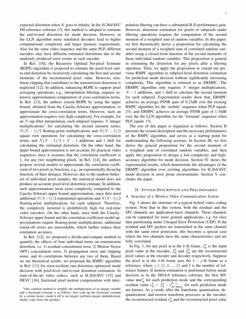
Fig. 1 shows the structure of a typical hybrid video codingsystem. Note that in this system, both the residual and theMV channels are application-layer channels. These channelscan be separated for more general applications, e.g. for slicedata partitioning under Unequal Error Protection (UEP). If theresidual and MV packets are transmitted in the same channelwith the same error protection, this becomes a special casewhere the two channels have the same characteristics and arefully correlated.

In Fig. 1, for any pixel u in the k-th frame, fku is the input

pixel value at the encoder; fku and fk

u are the reconstructedpixel values at the encoder and decoder respectively. Supposethe pixel u in the k-th frame uses the k − j-th frame as areference, where j ∈ 1, 2, ..., J and J is the number of ref-erence frames. If motion estimation is performed before modedecision as in the JM16.0 reference software, the best MVvalue mvk

u for each prediction mode and the correspondingresidual value eku = fk

u − fk−ju+mvk

ufor each prediction mode

are known. As a result, after the transform, quantization, de-quantization, and inverse transform processes at the encoder,the reconstructed residual eku and the reconstructed pixel value

3

Videocapture

Input

T/Q-Q-1/T-1

ResidualChannel

+

Motioncompensation

Memory

Motionestimation

MVChannel

Q-1/T-1

+

Motioncompensation

MV Errorconcealment

ChannelEncoder Decoder

Videodisplay

Output

Clipping Clipping

Memory

keu

kuvm

(

keuˆ

kfujkf −u

jkkf −

+ umvuˆ '

~~ jk

kf −+ uvmu

keu~

kfu

~

'~ jkf −u

Residual ErrorConcealment

keuˆ

keu(

kfu

kumv

S(r)

S(m)

‘0’

‘0’

‘1’

‘1’

Fig. 1. System structure, where T, Q, Q−1, and T−1 denote transform, quantization, inverse quantization, and inverse transform, respectively.

fku = Γ(fk−j

u+mvku+ eku) are known for each prediction mode.

Γ(·) is the clipping function and is defined by

Γ(x) =

γL, x < γL

x, γL ≤ x ≤ γH

γH , x > γH ,

(1)

where γL and γH are low threshold and high threshold ofpixel values. In this paper, we let γL = 0 and γH = 255.

Let us define fku − fk

u as quantization error and

ζku , fku − fk

u (2)

as transmission error. While the quantization error is knownto the encoder after the encoding process, the transmissionerror is caused from any combinations of three error events,i.e. residual packet, MV packet, and propagated errors. InFig. 1, the residual used for reconstruction in the decoder, i.e.eku, may be either the quantized residual eku or the concealedresidual eku depending on the error status of residual packetS(r); The MV used for motion compensation in the decoder,i.e. mv

ku, may be either the true MV mvk

u or the concealedMV mvk

u depending on the error status of MV packet S(m);as a result, the reconstructed pixel value in the decoder isfku = Γ(fk−j′

u+mvku

+ eku) where fk−j′

u+mvku

is the reference pixelvalue for reconstruction at the decoder, which recursivelydepends on all error events in the reference trajectory till theintra coded pixel.

Depending on whether the MV is correctly received or not,the propagated error can be calculated, according to (2), by

ζk−j′

u+mvku

=

ζk−ju+mvk

u= fk−j

u+mvku− fk−j

u+mvku, S(m)=0

ζk−j′

u+mvku= fk−j

u+mvku− fk−j′

u+mvku, S(m)=1,

(3)

where the concealed MV may point to a different referenceframe j′ from the true reference frame j.

Clipping noise is defined as ∆ku , (fk−j

u+mvku+ eku) −

Γ(fk−ju+mvk

u+ eku) at the encoder and as ∆k

u , (fk−j′

u+mvku

+

eku) − Γ(fk−j′

u+mvku

+ eku) at the decoder. That is, the clipping

noise at the decoder is a function of the residual concealment,MV concealment, and propagated errors. Denote r, m as theerror event that both residual and MV are correctly receivedat the decoder for pixel uk; the clipping noise under this eventwill be ∆k

ur, m = (fk−ju+mvk

u+ eku)− Γ(fk−j

u+mvku+ eku).

Some important notations used in this paper are listed inTable I. Throughout this paper, we addˆonto the reconstructedvariables at the encoder; addˇonto the concealed variables atthe decoder; and add˜onto the variables, which are subject tothe random channel error at the decoder.

B. Preliminaries about the RMPC algorithm

In Ref. [12], we take a divide-and-conquer approach to de-rive the second moment of ζku, i.e. E[(ζku)

2]. We first divide thetransmission reconstructed error into four components: threerandom errors (residual concealment, MV concealment, andpropagated errors) due to their different physical causes, andclipping noise, which is a non-linear function of these threerandom errors. This error decomposition allows us to quantifythe effects of below four terms on transmission distortion: (1)residual concealment error (R), (2) MV concealment error(M), (3) propagated error plus clipping noise (P), and (4)correlations between any two of the error sources (C). Basedon this decomposition, we developed a practical algorithm,called RMPC algorithm, to estimate the pixel-level end-to-enddistortion (PEED) for mode decision in Ref. [11].

In Ref. [11], the end-to-end distortion function for eachpixel u in the k-th frame is defined as Dk

u,ETE , E[(fku −

fku)

2], and can be derived by

Dku,ETE = E[(fk

u − fku)

2] = E[(fku − fk

u + ζku)2]

= (fku − fk

u)2 + E[(ζku)

2] + 2(fku − fk

u) · E[ζku].(4)

Define εku , eku−eku as the residual concealment error whenthe residual packet is lost; define ξku , fk−j

u+mvku− fk−j′

u+mvku

as the MV concealment error when the MV packet is lost;and denote P k

u as the PLP for pixel u in the k-th frame.Under the assumptions that S(r) is independent of eku and

4

TABLE INOTATIONS

fku : Value of the pixel with position u in the k-th frame, i.e. pixel uk .

eku : Residual value of the pixel uk .mvk

u : MV of the pixel uk .∆k

u : Clipping noise of the pixel uk .∆k

ur, m: Clipping noise of the pixel uk under the condition that both residual and MV are correctly received at the decoder.ζku : Transmission error of the pixel uk , defined in (2).εku : Residual concealment error of the pixel uk .ξku : MV concealment error of the pixel uk .ζk−j

u+mvku

: 1) propagated error of the pixel uk whose reference pixel is pointed to the k − j-th frame by the true MV mvku;

: 2) transmission error of the pixel with position u+mvku in the k − j-th frame according to (2).

ζk−j′

u+mvku

: 1) propagated error of the pixel uk whose reference pixel is pointed to the k − j′-th frame by the concealed MV mvku;

: 2) transmission error of the pixel with position u+ mvku in the k − j′-th frame according to (2).

S(m) is independent of ξku, i.e. the packet transmission erroris independent from the values of residual and MV, we provedin Refs. [12], [11] that without slice data partitioning, E[ζku]and E[(ζku)

2] can be calculated by (5) and (6) 2,

E[ζku] = P ku · (εku + ξku + E[ζk−j′

u+mvku])

+ (1− P ku ) · E[ζk−j

u+mvku+ ∆k

ur, m],(5)

E[(ζku)2] = P k

u · ((εku + ξku)2 + 2(εku + ξku) · E[ζk−j′

u+mvku]

+ E[(ζk−j′

u+mvku)2]) + (1− P k

u ) · E[(ζk−ju+mvk

u+ ∆k

ur, m)2],(6)

where E[ζk−j′

u+mvku] and E[(ζk−j′

u+mvku)2] in the k − j′-th frame

have been calculated by (5) and (6) and stored in memoryduring encoding of the k−j′-th frame; E[ζk−j

u+mvku+∆k

ur, m]and E[(ζk−j

u+mvku+ ∆k

ur, m)2] can be calculated by (7)

and (8), where E[ζk−ju+mvk

u] and E[(ζk−j

u+mvku)2] have been

calculated and stored in memory during encoding of the k−j-th frame. Note that in this paper, for simplicity, we use E(·)to also represent the estimate of E(·), i.e. E(·), in Ref. [11].

Existing pixel-level algorithms, e.g., the RMPC algorithm,are based on the integer pixel MV assumption to derive an esti-mate of Dk

u,ETE . In order words, in (5), (6), (7) and (8), mvku

is with integer-pixel accuracy. Therefore, their application instate-of-the-art encoders is limited due to the possible use offractional motion compensation. For subpixel motion compen-sation, E[ζk−j

u+mvku] and E[(ζk−j

u+mvku)2] need to be estimated

based on the interpolated pixel values, i.e. a weighted sumof several neighboring pixels. That is, E[(ζk−j

u+mvku)2] requires

the computation of the second moment of a weighted sum ofcorrelated random variables and therefore the computation ofseveral cross-correlation terms. This is also true for distortionestimation for pixels or subpixels under other filtering opera-tions. In Section III, we will extend RMPC algorithm to solvethis problem with low complexity.

III. THE EXTENDED RMPC ALGORITHM FOR MODEDECISION

In this section, we first derive a general proposition forany second moment of a weighted sum of correlated random

2In Ref. [12], [11], we assume that if S(m) = 1, the reference pixel,pointed by the concealed MV mvk

u, comes from the k − 1-th frame; inthis paper, we denote the k − j′-th frame for reference pixel pointed by theconcealed MV mvk

u without such an assumption.

variables; then we apply it to extend RMPC to estimate theend-to-end distortion for subpixel motion compensation anddesign the algorithm for mode decision.

A. Subpixel-level Distortion Estimation for Error ResilientVideo Encoding

Typically, the rate distortion optimized mode decision con-sists of two steps. First, the R-D cost is calculated by

J(ωm) = Dk(ωm) + λ ·R(ωm), (9)

where Dk = 1|Vk

l |∑

u∈VklDk

u; Vkl is the set of pixels in the

l-th MB (or sub-MB, i.e. any block size for a given predictionmode) of the k-th frame; ωm is the prediction mode [17];R(ωm) is the encoded bit rate for mode ωm, ωm ∈ Ωm andΩm is the mode set for mode decision; λ is the preset Lagrangemultiplier. Then, the optimal prediction mode that minimizesthe rate-distortion (R-D) cost is found by

ωm = arg minωm∈Ωm

J(ωm). (10)

For the RMPC algorithms, if the MV of one block forencoding is fractional, the MV has to be rounded to thenearest integer. This block will use the reference block pointedto by the rounded MV as a reference. However, in state-of-the-art codecs, such as H.264/AVC and HEVC, interpolationfilters are used to interpolate a reference block. Therefore, thedistortion of nearest neighbor approximation is not optimal forsuch an encoder. In order to optimally estimate the distortionfor pixels with interpolation filtering, or any other filtering ingeneral, we need to extend the existing RMPC algorithm.

In H.264/AVC, motion compensation accuracy is in unitsof one quarter of the distance between luma samples. 3 Theprediction values at half-sample positions are obtained byapplying a one-dimensional 6-tap Finite Impulse Response(FIR) filter horizontally and vertically. The prediction values atquarter-sample positions are generated by averaging samplesat integer- and half-sample positions [17]. Take ζk−j

u+mvku

in(5), (6), (7) and (8) for example. Denote vk−j = u + mvk

u

and v is in a subpixel position in the k − j-th frame. Allneighboring pixels in the integer position, used to interpolatethe reconstructed pixel value at v, are denoted by vi and witha weight wi, i ∈ 1, 2, ..., N , where N = 6 for the half-sample

3Note that considering the chroma distortion does not always improve theR-D performance but induces more complexity. Therefore, we only considerluma components in this paper.

5

E[ζk−ju+mvk

u+ ∆k

ur, m] =

fku − 255, E[ζk−j

u+mvku] < fk

u − 255

fku , E[ζk−j

u+mvku] > fk

u

E[ζk−ju+mvk

u], fk

u − 255 ≤ E[ζk−ju+mvk

u] ≤ fk

u ,

(7)

E[(ζk−ju+mvk

u+ ∆k

ur, m)2] =

(fk

u − 255)2, E[ζk−ju+mvk

u] < fk

u − 255

(fku)

2, E[ζk−ju+mvk

u] > fk

u

E[(ζk−ju+mvk

u)2], fk

u − 255 ≤ E[ζk−ju+mvk

u] ≤ fk

u ,

(8)

interpolation, and N = 2 for the quarter-sample interpolationin H.264/AVC. Therefore, the interpolated reconstructed pixelvalue at the encoder is

fk−jv =

N∑i=1

wi · fk−jvi

, (11)

and at the decoder

fk−jv =

N∑i=1

wi · fk−jvi

. (12)

From (2), we have

ζk−jv =

N∑i=1

wi · fk−jvi

−N∑i=1

wi · fk−jvi

=N∑i=1

wi · (fk−jvi

− fk−jvi

) =N∑i=1

wi · ζk−jvi

.

(13)

Since E[ζk−jvi

] has been calculated by the RMPC algorithm,E[ζk−j

v ] can be very easily calculated by

E[ζk−jv ] =

N∑i=1

wi · E[ζk−jvi

]. (14)

However, calculating E[(ζk−jv )2] is not straightforward since

E[(ζk−jv )2] = E[(

N∑i=1

wi · ζk−jvi

)2] (15)

is in fact the second moment of a weighted sum of correlatedrandom variables.

B. A Proposition for Calculating the Second Moment of aWeighted Sum of Correlated Random Variables

The Moment Generating Function (MGF) can be usedto calculate the second moment for random variables [18].However, to estimate the second moment of a weighted sum ofrandom variables, the traditional moment generating functionusually requires knowing their probability distribution andassumes they are independent. However, in a practical videocodec, most random variables, e.g. those involved in theaveraging operations, are not independent and their probabilitydistributions are unknown. Therefore, some approximations,such as the Cauchy-Schwarz upper bound approximation [13]or the correlation coefficient model approximation [14], areusually adopted. However, those approximations are of highcomplexity. For example, for each subpixel, with the N -tapfilter interpolation, the Cauchy-Schwarz upper bound approx-imation requires N integer multiplications for calculating thesecond moment terms, N(N − 1)/2 floating-point multipli-cations and N(N − 1)/2 square root operations for calculat-ing the cross-correlation terms, and N(N − 1)/2 + N − 1

additions and 1 shift for calculating the estimated distor-tion. The correlation coefficient model requires an additionalN(N−1)/2 exponential operations and N(N−1)/2 floating-point multiplications when compared to the Cauchy-Schwarzupper bound approximation.

In a wireless video communication system, the computa-tional capability of the real-time encoder is usually very lim-ited, and floating-point processing is undesirable. Therefore,it is desirable to design a new algorithm for the calculationof the second moment in (15) using only integer operations.Proposition 1 is a result of this motivation.

Proposition 1: For any N correlated random variablesX1, X2, ..., XN and wi ∈ ℜ, i ∈ 1, 2, ..., N, the secondmoment of the weighted sum of these random variables isgiven by (16).

E[(

N∑i=1

wi ·Xi)2] =

N∑i=1

wi ·N∑j=1

[wj · E(X2j )]−

N−1∑k=1

N∑l=k+1

[wk · wl · E(Xk −Xl)2]

(16)

The proof of Proposition 1 is provided below. Note that inH.264/AVC, most averaging operations, e.g., interpolation, de-blocking, and bi-prediction, are special cases of Proposition 1in that

∑Ni=1 wi = 1. Therefore, we can extend the RMPC

algorithm through the consideration of Proposition 1. In (16),since E(X2

j ) has been estimated by the RMPC algorithm,the only unknown is

∑N−1k=1

∑Nl=k+1[wk ·wl ·E(Xk −Xl)

2].However, we will see that this unknown can be assumed to benegligible for the purposes of mode decision.

C. The Extended RMPC Algorithm for Mode Decision

1) Algorithm design: Replacing Xk and Xl in (16) by ζkui

and ζkuj, and from (2) we have

E[(Xk −Xl)2] = E[(ζkui

− ζkuj)2]

= E[fkui

− fkui

− (fkuj

− fkuj)]2

= E[(fkui

− fkuj)− (fk

ui− fk

uj)]2.

(17)

In (17), both fkui−fk

ujand fk

ui−fk

ujdepend on the spatial cor-

relation of the reconstructed pixel values in position ui and uj .When ui and uj are located in the same neighborhood, theyare very likely to be transmitted in the same packet. In otherwords, either both fk

uiand fk

ujuse the true MV and residual

for reconstruction, or both fkui

and fkuj

use the concealed MVand residual for reconstruction. Therefore, fk

ui− fk

ujwill not

change too much from fkui

− fkuj

, and hence E[(ζkui− ζkuj

)2]

6

Proof:

E[(N∑i=1

wi ·Xi)2] = E[

N∑j=1

(w2j ·X2

j ) +N∑

k=1

N∑l=1

(l=k)

(wk · wl ·Xk ·Xl)]

= E[N∑

j′=1

wj′

N∑j=1

(wj ·X2j )−

N∑j=1

N∑j′=1

(j′ =j)

(wj · wj′ ·X2j ) +

N∑k=1

N∑l=1

(l=k)

(wk · wl ·Xk ·Xl)]

=N∑i=1

wi

N∑j=1

[wj · E(X2j )]− E

N−1∑k=1

N∑l=k+1

[wk · wl · (X2k +X2

l )] +N−1∑k=1

N∑l=k+1

(2 · wk · wl ·Xk ·Xl)

=N∑i=1

wi

N∑j=1

[wj · E(X2j )]−

N−1∑k=1

N∑l=k+1

[wk · wl · E(Xk −Xl)2].

is much smaller than E[(ζkui)2] and E[(ζkuj

)2] in (16). Onthe other hand, distortion is estimated for one MB or onesub-MB as in (9) for mode decision. When the cardinality|Vk

l | is large,∑

v∈Vkl

∑N−1i=1

∑Nj=i+1[wi ·wj ·E(ζkui

− ζkuj)2]

converges to a constant for all modes with high probability dueto the summation over the same samples in each mode. Forsimplicity, we will call it “negligible term” in the followingsections. Therefore, in (16) only the first term on the right-hand side needs to be calculated without too much loss inprecision.

Since∑N

i=1 wi = 1, we calculate E[(ζkv)2] for mode

decision by

E[(ζkv)2] =

N∑i=1

[wi · E(ζkui)2]. (18)

With the N -tap filter interpolation, the complexity in (18)is dramatically reduced to only N integer multiplications,N − 1 additions, and 1 shift. Here, we propose the followingalgorithm to extend the RMPC algorithm for mode decision.

Algorithm 1: Rate distortion optimized mode decision foran MB in the k-th frame (k >= 1).

1) Input: QP, PLP.2) Initialization of E[ζ0u] and E[(ζ0u)

2] for all pixel u.3) Loop for all available modes for each MB.

3a) estimate E[ζk−ju+mvk

u] via (14) and

E[(ζk−ju+mvk

u)2] via (18) for all pixels in the MB,

3b) estimate E[ζk−ju+mvk

u+ ∆k

ur, m] via (7) and

E[(ζk−ju+mvk

u+ ∆k

ur, m)2] via (8) for all pixelsin the MB,3c) estimate E[ζku] via (5) and E[(ζku)

2] via (6)for all pixels in the MB,3d) estimate Dk

u via (4) for all pixels in the MB,3e) estimate R-D cost for the MB via (9),

End4) Via (10), select the best mode with minimum R-Dcost for the MB.5) Output: the best mode for the MB.

Algorithm 1 is referred to as the Extended RMPC(ERPMC). Note that if an MV packet is lost, in order toreduce both the MV concealment and distortion estimationcomplexity, the concealed MV mvk

u does not necessary usefractional accuracy. That is, the ERMPC algorithm conceals

the MV with integer accuracy. Therefore, E[ζk−j′

u+mvku] and

E[(ζk−j′

u+mvku)2] in (5) and (6) do not require (18).

2) Complexity analysis: In Ref. [11], we compare thecomplexity of RMPC to that of ROPE and LLN in the-ory. In this section, we first compare the complexity ofERMPC to RMPC in theory. Then, we test the complexityof ERMPC/RMPC/ROPE in JM16.0 and compare them to thedefault ERRDO algorithm in JM16.0, i.e. LLN; we also testthe RDO without error-resilient algorithms as a benchmark.

RMPC computational complexity is calculated from (4),(5), (6), (7) and (8), where the first moment and the secondmoment of the reconstructed error of the best mode shouldbe stored after the mode decision (Note that the reconstructederror in previous frames could be regarded as the propagatederror in the current frame, recursively). Therefore, 2 units ofmemory are required to store those two moments for eachpixel. Note that the first moment E[ζk−j

u+mvku] takes values

in −255,−254, ..., 255, i.e., 8 bits plus 1 sign bit perpixel, and the second moment E[(ζk−j

u+mvku)2] takes values

in 0, 1, ..., 2552, i.e., 16 bits per pixel. From the discus-sion above, we know that the difference, in computationalcomplexity, of ERMPC compared to RMPC is the estimationof E[ζk−j

u+mvku] in (7) and E[(ζk−j

u+mvku)2] in (8). To be more

specific, in ERMPC E[ζk−ju+mvk

u] and E[(ζk−j

u+mvku)2] include a

fractional MV while in RMPC E[ζk−ju+mvk

u] and E[(ζk−j

u+mvku)2]

include only an integer MV. Therefore, the additional complex-ity of ERMPC compared to RMPC is the calculation of (14)and (18).

Note that (14) and (18) are not needed in ERMPC if: 1)the prediction mode is intra; 2) the MV is an integer MV. ForMVs pointing to half-pixel positions, the values of wi are1,−5, 20, 20,−5, 1 in (14) and (18); i.e., there are N = 6integer multiplications, N − 1 = 5 additions, and 1 right shiftwith 5 bits to make sure

∑Ni=1 wi = 1. By using the same

simplification of the JM interpolation implementation, (18) canbe calculated by E(ζku3.5

)2 = 20 · [E(ζku3)2 +E(ζku4

)2]− 5 ·[E(ζku2

)2 + E(ζku5)2] + [E(ζku1

)2 + E(ζku6)2] + 16 >> 5.

In fact, we may further simplify the implementation of (18)by replacing the integer multiplication operations by additions

7

and shifts as

E(ζku3.5)2 = [E(ζku3

)2 + E(ζku4)2] ≪ 4

+ [E(ζku3)2 + E(ζku4

)2] ≪ 2− [E(ζku2)2 + E(ζku5

)2] ≪ 2

− [E(ζku2)2 + E(ζku5

)2] + [E(ζku1)2 + E(ζku6

)2] + 16 ≫ 5.(19)

Note that in (19), E(ζku3)2+E(ζku4

)2 and E(ζku2)2+E(ζku5

)2

are invoked two times, but are counted only once since thetemporary result is saved in the CPU register. As a result, thehalf-pixel position needs 8 additions (ADDs) and 4 shifts only.

For quarter-pixel positions additional computations willneed to be performed. We observe that there are two prac-tical implementations for ERMP, each one having differentcomputational complexity and memory requirements. In thefirst, we can store the first and second moments of thetransmission error for half-pixel positions, which will require3 times the memory compared to storing only the integerpixel moments. However, this will reduce the complexity ofcalculating the moments for quarter-pixel positions. In thesecond, the moments for all fractional positions are calculatedon the fly. This is also the method used in the LLN algorithmavailable in the JM. The complexity of this method is analyzedbelow. Note that the computational complexity of calculating(14) and (18) for different subpixel positions is different.

In this paper we only show the complexity analysis forthose half-pixel positions interpolated by integer pixels. It isvery easy to extend this analysis for all fractional positions.Since (14) and (18) are calculated on the fly, there is noadditional memory requirement for ERMPC. Note that in mostCPUs, a shift can be integrated into an ADD, therefore notimpacting complexity. As a result, the complexity of ERMPCcan be found in Table II 4. For LLN, half-pixel positionmotion compensation requires 8 ADDs and 4 shifts more thanLLN with integer-pixel position motion compensation for eachsimulated decoder; that is LLN is 8Nd ADDs more than thecomplexity of that in Ref. [11], where Nd means the numberof simulated decoders at the encoder; the default value in JM isNd = 30. We also cite the complexity of ROPE and LLN withinteger MV accuracy from Ref. [11] in Table II for reference.

Since the theoretical complexity comparison only accountsfor half-pixel positions, it would be beneficial to evaluate com-plexity in a real encoding environment. In reality, MVs couldpoint to any position, integer or fractional. The nearest integerMV is used to approximate the fractional MV in RMPC andROPE. NO ERRDO means the normal RDO mode decisionprocess, without any error resiliency considerations availablein the JM. Table III shows the results for the mobile sequenceat CIF resolution with PLP = 5%. The experimental setup isthe same as those in Section IV. A system based on an AMDOpteron(tm) 2356 processor at 2.29GHz was used. It can beseen that the executation time of ERMPC/RMPC/ROPE isonly slightly higher of that of ERRDO. However, LLN requiresconsiderable more execution time than these schemes. Othersequences and channel conditions show similar results.

4Note that in H.264/AVC seven inter prediction modes are supported, i.e.,16× 16, 16× 8, 8× 16, 8× 8, 8× 4, 4× 8, and 4× 4. Nine intra 4× 4and 8 × 8 modes, as well as four 16 × 16 modes for luma intra predictionare supported. Total complexity is calculated for all prediction modes.

D. Merits and Limitations of ERMPC Algorithm

1) Merits: Since both the Cauchy-Schwarz upper boundapproximation [13] and the correlation coefficient model ap-proximation [14] induce floating-point multiplications, round-off error is unavoidable. The algorithm by Yang et al. [14]needs extra complexity to mitigate the effect of round-off errorduring distortion estimation. In contrast, one of the merits ofProposition 1 is that it only needs integer multiplications andadditions. In H.264/AVC and HEVC, wi (and wi ·wj) can bescaled to an integer value without any round-off error for allcoding modes. As a result, round-off error can be avoided inthe ERMPC algorithm.

In Ref. [19], the authors prove that a low-pass interpolationfilter will decrease the frame-level propagated error undersome assumptions. In fact, it is easy to prove that when∑N

i=1 wi = 1 and |Vkl | is large, the negligible term is larger

than or equal to zero. Even at the MB-level, the negligibleterm is larger than or equal to zero with very high probability.From (16), we see that the block-level distortion decreases,with very high probability, after the interpolation filtering.

One additional benefit of (16) is to guide the design of theinterpolation filter. Traditional interpolation filter design aimsto minimize the prediction error. With (16), we may designan interpolation filter by maximizing

∑Nk=1

∑Nl=k+1[wk ·wl ·

E(Xk −Xl)2] under the constraint of

∑Nj=1[wj · E(X2

j )].2) Limitations: In Algorithm 1, the second moment of

propagated error E[(ζk−ju+mvk

u)2] is estimated by ignoring the

negligible term to reduce the complexity. A more accuratealternative method is to estimate E(ζkui

− ζkuj)2] recursively

by storing the value in memory. This will be considered inour future work.

IV. EXPERIMENTAL RESULTS

In this section, we compare the R-D performance andsubjective performance of the ERMPC algorithm with thatof the RMPC and the LLN algorithms for mode decision inH.264/AVC. Since the original ROPE does not support theinterpolation filtering operation and its extensions [13], [14]induce many floating-point operations and round-off errors, weonly use the same nearest integer MV approximation to showhow its R-D performance differs from ERMPC, RMPC, andLLN. To compare all algorithms under multi-reference picturemotion compensated prediction, we also enhance the originalROPE algorithm [10] with multi-reference capability.

A. Experimental Setup

The JM encoder and decoder were used in the experiments.The first 100 frames from several CIF resolution, 30fps testvideo sequences were tested under different PLP settings from0.5% to 5%. The co-located pixel copy from the previousframe method was used for error concealment in all algo-rithms. The first frame is assumed to be correctly received.The High profile of H.264/AVC, using CABAC for entropycoding but without B slices, with 3 slices per picture and 3reference frames, was used. Constrained intra prediction wasalso enabled. In the LLN algorithm, the number of simulateddecoders is 30.

8

TABLE IICOMPLEXITY COMPARISON IN THEORY

Algorithms computational complexity memory requirementinter mode 25 ADDs, 8 MULs

ERMPC (half-pixel) intra mode 7 ADDs, 6 MULs 25 bits/pixeltotal complexity 266 ADDs, 134 MULs

inter mode 9 ADDs, 8 MULsRMPC intra mode 7 ADDs, 6 MULs 25 bits/pixel

total complexity 154 ADDs, 134 MULsinter mode 10Nd ADDs, Nd MULs

LLN (half-pixel) intra mode Nd ADDs, Nd MULs 8Nd bits/pixeltotal complexity 83Nd ADDs, 20Nd MULs

inter mode 2Nd ADDs, Nd MULsLLN (integer pixel) intra mode Nd ADDs, Nd MULs 8Nd bits/pixel

total complexity 27Nd ADDs, 20Nd MULsinter mode 7 ADDs, 8 MULs

ROPE intra mode 4 ADDs, 7 MULs 24 bits/pixeltotal complexity 101 ADDs, 147 MULs

TABLE IIICOMPLEXITY COMPARISON IN EXPERIMENT

Algorithm ERMPC RMPC LLN ROPE NO ERRDOTime in second 105.828 105.126 137.393 104.766 102.719

B. R-D Performance

Due to space limitations, we only show the plots of PSNRvs. bit rate for video sequences ‘foreman’ and ‘mobile’ underPLP = 0.5% and PLP = 2% in Figs. 2 and 3 respectively.The experimental results show that ERMPC achieves thebest R-D performance; RMPC achieves the second best R-D performance; ROPE achieves better performance than LLNin some cases such as at high rate in Fig. 2, but worseperformance than LLN in other cases such as in Fig. 3 and atthe low rate in Fig. 2.

It is interesting to see that for some sequences and chan-nel conditions, ERMPC achieves a notable PSNR gain overRMPC. This is, for example, evident in ‘mobile’ and ‘fore-man’. For some other cases, however, ERMPC only achievesa marginal PSNR gain over RMPC (e.g., ‘coastguard’ and‘football’). From the analysis in Section III-A, we knowthat the only difference between RMPC and ERMPC is theestimate of the propagated error ζk−j

u+mvku

in (7) and (8).Therefore, the performance gain of ERMPC over RMPC onlycomes from inter modes, since they both use exactly the sameestimates for intra modes. Thus, the higher percentage of intramodes in ‘coastguard’ and ‘football’ may result in a marginalPSNR gain of ERMPC over RMPC.

For most sequences and channel conditions, we observe thatin most cases the higher the bit rate for encoding, the morethe PSNR gain of ERMPC over RMPC, such as in Fig. 2and Fig. 3(a). In (4), the end-to-end distortion consists ofboth quantization and transmission distortion. The ERMPCalgorithm gives a more accurate estimation of propagated errorin transmission distortion than the RMPC algorithm. When thebit rate for source encoding is very low, with rate control thecontrolled Quantization parameter (QP) is large, and hencethe quantization distortion becomes the dominant part in theend-to-end distortion. Therefore, the PSNR gain of ERMPCover RMPC is marginal. On the contrary, when the bit rate forsource encoding is high, the transmission distortion becomesthe dominant part in the end-to-end distortion. Therefore, thePSNR gain of ERMPC over RMPC is notable. However, thisis not always true as observed in Fig. 3(b). The reason isas follows. In the JM, the Lagrange multiplier in (9) is a

function of QP. A higher bit rate or smaller QP also causesa smaller Lagrange multiplier; therefore, the rate cost in (9)becomes smaller, which may produce a higher percentageof intra modes. In such a case, the PSNR gain of ERMPCover RMPC decreases. As a result, different sequences givedifferent results depending on whether the effect of increaseof intra modes dominates over the effect of decrease ofquantization distortion.

LLN has poorer R-D performance than ERMPC. This maybe since 30 simulated decoders are still not enough to achieve areliable distortion estimate. Meanwhile, complexity increase isconsiderable compared to ERMPC. It is also interesting to seethat the integer MV approximation for ROPE is only valid forsome sequences, such as ‘foreman’, while this approximationgives poor R-D performance for some other sequences, suchas ‘mobile’. However, the nearest neighbor approximation forRMPC in all sequences achieves good performance. This isbecause RMPC approximates the first and second moments ofthe propogated error ζk−j

u+mvku

by the rounded MV, while ROPEapproximates the first and second moments of the referencepixel value fk−j

u+mvku

by the rounded MV. Since the propagatederrors are much smaller and more stable than the referencepixel values, RMPC shows better and more stable performanceusing integer MV approximation.

Table IV shows the average PSNR gain (in dB) of ERMPCover RPMC, LLN, and ROPE for different video sequencesand different PLP. The average PSNR gain is obtained usingthe BD-PSNR method in Ref. [20], which measures theaverage distance (in PSNR) between two R-D curves. FromTable IV, we see that ERMPC achieves an average PSNRgain of 0.25dB over RMPC for the sequence ‘mobile’ underPLP = 2%; it achieves an average PSNR gain of 1.34dBover LLN for the ‘foreman’ sequence under PLP = 1%; andit achieves an average PSNR gain of 3.18dB over ROPE forthe ‘mobile’ sequence under PLP = 0.5%.

C. Subjective Performance

Since PSNR may not be as meaningful for error conceal-ment, subjective performance is also evaluated. Fig. 4 showsthe subjective quality of the 84-th frame and the 99-th frameof ‘foreman’ sequence under a PLP of 1% and a bit rate of

9

200 400 600 800 1000 1200 1400 1600 1800 200031

32

33

34

35

36

37

38

39

40

41

Bit rate (kb/s)

PS

NR

(dB

)

RMPCROPELLNERMPC

200 400 600 800 1000 1200 1400 1600 1800 2000 220030

31

32

33

34

35

36

37

38

39

Bit rate (kb/s)

PS

NR

(dB

)

RMPCROPELLNERMPC

(a) (b)Fig. 2. PSNR vs. bit rate for ‘foreman’: (a) PLP=0.5%, (b) PLP=2%.

200 400 600 800 1000 1200 1400 1600 1800 2000 220023

24

25

26

27

28

29

30

31

32

33

Bit rate (kb/s)

PS

NR

(dB

)

RMPCROPELLNERMPC

200 400 600 800 1000 1200 1400 1600 1800 2000 220022

23

24

25

26

27

28

29

30

Bit rate (kb/s)

PS

NR

(dB

)

RMPCROPELLNERMPC

(a) (b)Fig. 3. PSNR vs. bit rate for ‘mobile’: (a) PLP=0.5%, (b) PLP=2%. TABLE IV

AVERAGE PSNR GAIN (IN DB) OF ERMPC OVER RMPC, LLN AND ROPESequence coastguard football foreman mobile

PLP 5% 2% 1% 0.5% 5% 2% 1% 0.5% 5% 2% 1% 0.5% 5% 2% 1% 0.5%ERMPC vs. RMPC 0.09 0.08 0.08 0.06 0.01 0.01 0.01 0.03 0.08 0.13 0.21 0.17 0.20 0.25 0.21 0.21ERMPC vs. LLN 0.32 0.36 0.46 0.37 0.28 0.39 0.36 0.26 0.64 1.07 1.34 1.24 0.50 0.82 0.56 0.54

ERMPC vs. ROPE 0.58 0.46 0.52 0.62 0.47 0.25 0.27 0.33 1.59 1.37 1.41 1.42 1.11 1.89 2.79 3.18

250kbps. These results suggest a similar performance as thosepresented in Section IV-B. We can thus conclude that ERMPCachieves the best performance.

D. Discussion

1) Effect of clipping noise on the mode decision: SinceROPE does not consider the effect of clipping noise onthe transmission distortion, it over-estimates the end-to-enddistortion for inter modes. Hence, ROPE would tend to selectintra modes more often than ERMPC, RMPC, and LLN, whichwill lead to higher encoding bit rates. To verify this conjecture,we tested all sequences under the same QP settings, from 20 to32, without rate control. We observed that the ROPE algorithmalways produced a higher bit rate than other schemes as shownin Fig. 5 and Fig. 6.

2) Effect of transmission errors on mode decision: One canobserve three characteristics for ERMPC/RMPC/LLN/ROPE

algorithms vs NO ERRDO. 1) The number of intra MBsincreases since the transmission error is accounted for duringmode decision; 2) The number of skip mode MBs alsoincreases, since the transmission error will increase the trans-mission distortion in all other modes except for this mode; 3)if we allow the first frame to be erroneous, the second framewill have high percentage of intra MBs. This is because onlythe value of 128 can be used to conceal the reconstructed pixelvalues if the first frame is lost, while if other frames are lost thecollocated pixel in the previous frame can be used to concealthe reconstructed pixel values. Therefore, the propagated errorfrom the first frame will be much higher than the error fromother frames. As a result, if the first frame is allowed to belost with a certain probability, the second frame will containa high percentage of intra MBs due to ERRDO.

10

(a) (b) (c) (d)

(e) (f) (g) (h)Fig. 4. (a) ERMPC at the 84-th frame, (b) RMPC at the 84-th frame, (c) LLN at the 84-th frame, (d) ROPE at the 84-th frame, (e) ERMPC at the 99-thframe, (f) RMPC at the 99-th, (g) LLN at the 99-th frame, (h) ROPE at the 99-th frame.

0 500 1000 1500 2000 2500 3000 350033

34

35

36

37

38

39

40

41

42

Bit rate (kb/s)

PS

NR

(dB

)

RMPCROPELLNERMPC

0 500 1000 1500 2000 2500 3000 3500 400031

32

33

34

35

36

37

38

39

40

Bit rate (kb/s)

PS

NR

(dB

)

RMPCROPELLNERMPC

(a) (b)Fig. 5. PSNR vs. bit rate for ‘foreman’: (a) PLP=0.5%, (b) PLP=2%.

V. CONCLUSION

In this paper, we proved a new proposition for calculatingthe second moment of a weighted sum of correlated randomvariables without requiring knowledge of the random vari-able probability distributions. Then, we apply this proposi-tion to extend our previous RMPC algorithm in estimatingthe fractional-level end-to-end distortion for prediction modedecision without significantly increasing complexity. Experi-mental results show that ERMPC achieves on average a PSNRgain of 0.25dB over the existing RMPC algorithm for the‘mobile’ sequence when PLP equals 2%; ERMPC achieves anaverage PSNR gain of 1.34dB over the the LLN algorithm forthe ‘foreman’ sequence when PLP equals 1%. Experimentalresults also show that subjective quality was also improved.

REFERENCES

[1] C. E. Shannon, “Coding theorems for a discrete source with a fidelitycriterion,” IRE Nat. Conv. Rec. Part, vol. 4, pp. 142–163, 1959.

[2] T. Berger, Rate distortion theory: A mathematical basis for data com-pression. Prentice-Hall, Englewood Cliffs, NJ, 1971.

[3] Y. Shoham and A. Gersho, “Efficient bit allocation for an arbitrary set ofquantizers.” IEEE Trans. Acoust. Speech Signal Process., vol. 36, no. 9,pp. 1445–1453, 1988.

[4] H. Everett III, “Generalized Lagrange multiplier method for solvingproblems of optimum allocation of resources,” Operations Research,vol. 11, no. 3, pp. 399–417, 1963.

[5] A. Ortega and K. Ramchandran, “Rate-distortion methods for image andvideo compression,” IEEE Signal Processing Magazine, vol. 15, no. 6,pp. 23–50, 1998.

[6] G. Sullivan and T. Wiegand, “Rate-distortion optimization for videocompression,” IEEE Signal Processing Magazine, vol. 15, no. 6, pp.74–90, 1998.

[7] “H.264/AVC reference software JM16.0,” Jul. 2009. [Online]. Available:http://iphome.hhi.de/suehring/tml/download

[8] T. Stockhammer, M. Hannuksela, and T. Wiegand, “H. 264/AVC inwireless environments,” IEEE Transactions on Circuits and Systems forVideo Technology, vol. 13, no. 7, pp. 657–673, 2003.

[9] T. Stockhammer, T. Wiegand, and S. Wenger, “Optimized transmissionof h.26l/jvt coded video over packet-lossy networks,” in IEEE ICIP,2002.

[10] R. Zhang, S. L. Regunathan, and K. Rose, “Video coding with optimalinter/intra-mode switching for packet loss resilience,” IEEE Journal onSelected Areas in Communications, vol. 18, no. 6, pp. 966–976, Jun.2000.

[11] Z. Chen and D. Wu, “Prediction of Transmission Distortion for WirelessVideo Communication: Algorithm and Application,” Journal of VisualCommunication and Image Representation, vol. 21, no. 8, pp. 948–964,2010.

11

0 2000 4000 6000 8000 10000 1200028

30

32

34

36

38

40

42

Bit rate (kb/s)

PS

NR

(dB

)

RMPCROPELLNERMPC

0 2000 4000 6000 8000 10000 1200026

28

30

32

34

36

38

Bit rate (kb/s)

PS

NR

(dB

)

RMPCROPELLNERMPC

(a) (b)Fig. 6. PSNR vs. bit rate for ‘mobile’: (a) PLP=0.5%, (b) PLP=2%.

[12] ——, “Prediction of Transmission Distortion for Wireless Video Com-munication: Part I: Analysis,” IEEE Transactions on Image Processing,2011, accepted.

[13] A. Leontaris and P. Cosman, “Video compression for lossy packet net-works with mode switching and a dual-frame buffer,” IEEE Transactionson Image Processing, vol. 13, no. 7, pp. 885–897, 2004.

[14] H. Yang and K. Rose, “Advances in recursive per-pixel end-to-enddistortion estimation for robust video coding in H. 264/AVC,” IEEETransactions on Circuits and Systems for Video Technology, vol. 17,no. 7, p. 845, 2007.

[15] ITU-T Series H: Audiovidual and Multimedia Systems, Advanced videocoding for generic audiovisual services, Nov. 2007.

[16] T. Wiegand, W.-J. Han, B. Bross, J.-R. Ohm, and G. J. Sullivan, WD1:Working Draft 1 of High-Efficiency Video Coding, Guangzhou, Oct.2010, JCTVC-C403, 3rd JCT-VC Meeting.

[17] T. Wiegand, G. J. Sullivan, G. Bjontegaard, and A. Luthra, “Overview ofthe h.264/AVC video coding standard,” IEEE Transactions on Circuitsand Systems for Video Technology, vol. 13, no. 7, pp. 560–576, Jul.2003.

[18] G. Casella and R. L. Berger, Statistical Inference, 2nd ed. DuxburyPress, 2001.

[19] K. Stuhlmuller, N. Farber, M. Link, and B. Girod, “Analysis of videotransmission over lossy channels,” IEEE Journal on Selected Areas inCommunications, vol. 18, pp. 1012–1032, Jun. 2000.

[20] G. Bjontegaard, “Calculation of average PSNR differences between RD-curves, 13th VCEG-M33 Meeting,” Austin, USA, 2001.

Zhifeng Chen received Ph.D. degree in Electricaland Computer Engineering from the University ofFlorida, Gainesville, Florida, in 2010. From 2002to 2003, he was an engineer in EPSON (China),and from 2003 to 2006, he was a senior engineerin Philips (China), both working in mobile phonesystem solution design. He joined Interdigital Inc. in2010, where he is currently a staff engineer workingon video coding research.

Peshala V. Pahalawatta received his Ph.D. degreein electrical engineering from Northwestern Uni-versity, Evanston, IL, in 2007. He is currently aStaff Engineer with the Image Technology group atDolby Laboratories Inc., Burbank, CA. His researchinterests include image and video compression andtransmission, image and video quality evaluation,and computer vision.

Alexis M. Tourapis received the Diploma degreein Electrical and Computer Engineering from theNational Technical University of Athens (NTUA),Greece, in 1995 and the Ph.D. degree in Elec-trical and Electronic Engineering from the HongKong University of Science & Technology, HK, in2001. Alexis has held in the past various researchand development positions with companies suchas Microsoft, Thomson, DoCoMo Labs USA, andDolby Laboratories. He is currently with MagnumSemiconductor Inc. as a Senior Director of Video

Algorithm Engineering focusing on the development of next generation videoprocessing and compression hardware system designs.

Alexis is a senior member of the IEEE, and a member of the ACM, SPIE,and SMPTE. In 2000 he received the IEEE HK section best postgraduatestudent paper award for his work, and in 2006 he was acknowledged asone of 10 most outstanding reviewers by the IEEE Transactions on ImageProcessing. Alexis currently holds 7 US patents and has more than 90 USand international patents pending. Alexis has made several contributions toseveral video coding standards, and in particular to H.264/MPEG-4 AVC, on avariety of topics, such as motion estimation and compensation, rate distortionoptimization, rate control and others, and currently serves as a co-chair of thedevelopment activity on the H.264 Joint Model (JM) reference software.

Dapeng Wu (S’98–M’04–SM’6) received Ph.D. inElectrical and Computer Engineering from CarnegieMellon University, Pittsburgh, PA, in 2003. Cur-rently, he is a professor of Electrical and ComputerEngineering Department at University of Florida,Gainesville, FL.