March 2001

NASA/TM-2001-210838

Improved Equivalent Linearization Implementations Using Nonlinear Stiffness Evaluation Stephen A. Rizzi and Alexander A. Muravyov Langley Research Center, Hampton, Virginia

The NASA STI Program Office ... in Profile

Since its founding, NASA has been dedicated to the advancement of aeronautics and space science. The NASA Scientific and Technical Information (STI) Program Office plays a key part in helping NASA maintain this important role.

The NASA STI Program Office is operated by Langley Research Center, the lead center for NASA�s scientific and technical information. The NASA STI Program Office provides access to the NASA STI Database, the largest collection of aeronautical and space science STI in the world. The Program Office is also NASA�s institutional mechanism for disseminating the results of its research and development activities. These results are published by NASA in the NASA STI Report Series, which includes the following report types:

• TECHNICAL PUBLICATION. Reports of

completed research or a major significant phase of research that present the results of NASA programs and include extensive data or theoretical analysis. Includes compilations of significant scientific and technical data and information deemed to be of continuing reference value. NASA counter-part of peer reviewed formal professional papers, but having less stringent limitations on manuscript length and extent of graphic presentations.

• TECHNICAL MEMORANDUM. Scientific

and technical findings that are preliminary or of specialized interest, e.g., quick release reports, working papers, and bibliographies that contain minimal annotation. Does not contain extensive analysis.

• CONTRACTOR REPORT. Scientific and

technical findings by NASA-sponsored contractors and grantees.

• CONFERENCE PUBLICATION. Collected papers from scientific and technical conferences, symposia, seminars, or other meetings sponsored or co-sponsored by NASA.

• SPECIAL PUBLICATION. Scientific,

technical, or historical information from NASA programs, projects, and missions, often concerned with subjects having substantial public interest.

• TECHNICAL TRANSLATION. English-

language translations of foreign scientific and technical material pertinent to NASA�s mission.

Specialized services that help round out the STI Program Office�s diverse offerings include creating custom thesauri, building customized databases, organizing and publishing research results ... even providing videos. For more information about the NASA STI Program Office, see the following: • Access the NASA STI Program Home

Page at http://www.sti.nasa.gov • E-mail your question via the Internet to

help@sti.nasa.gov • Fax your question to the NASA Access Help

Desk at (301) 621-0134 • Phone the NASA Access Help Desk at (301)

621-0390 • Write to:

NASA Access Help Desk NASA Center for AeroSpace Information 7121 Standard Drive Hanover, MD 21076-1320

National Aeronautics and Space Administration Langley Research Center Hampton, Virginia 23681-2199

March 2001

NASA/TM-2001-210838

Improved Equivalent Linearization Implementations Using Nonlinear Stiffness Evaluation Stephen A. Rizzi and Alexander A. Muravyov Langley Research Center, Hampton, Virginia

A N7H(

The use of trademarks or names of manufacturers in the report is for accurate reporting and does not constitute an official endorsement, either expressed or implied, of such products or manufacturers by the National Aeronautics and Space Administration.

vailable from the following:

ASA Center for AeroSpace Information (CASI) National Technical Information Service (NTIS) 121 Standard Drive 5285 Port Royal Road anover, MD 21076-1320 Springfield, VA 22161-2171

301) 621-0390 (703) 487-4650

i

Foreword This report documents two new implementations of equivalent linearization for solving geometrically nonlinear random vibration problems of complicated structures. The implementations are given the acronym ELSTEP, for �Equivalent Linearization using a STiffness Evaluation Procedure.� Both implementations of ELSTEP are fundamentally the same in that they use a novel nonlinear stiffness evaluation procedure to numerically compute otherwise inaccessible nonlinear stiffness terms from commercial finite element programs. The commercial finite element program MSC/NASTRAN (NASTRAN) was chosen as the core of ELSTEP. The FORTRAN implementation calculates the nonlinear stiffness terms and performs the equivalent linearization analysis outside of NASTRAN. The Direct Matrix Abstraction Program (DMAP) implementation performs these operations within NASTRAN. Both provide nearly identical results. Within each implementation, two error minimization approaches for the equivalent linearization procedure are available � force and strain energy error minimization. Sample results for a simply supported rectangular plate are included to illustrate the analysis procedure.

The majority of this work was originally performed by Alexander A. Muravyov during his tenure as a National Research Council post-doctoral research associate at the NASA Langley Research Center. Additional enhancements and interfaces were subsequently developed by Stephen A. Rizzi. The authors wish to thank Jay H. Robinson and Travis L. Turner of the Structural Acoustics Branch at the NASA Langley Research Center for helpful discussions and comments.

ii

Table of Contents 1. Introduction ....................................................................................................................................... 1-1 2. Finite Element Model Development ................................................................................................. 2-1

2.1. Normal Modes Analysis Bulk Data File ................................................................................... 2-1 2.2. Static Analysis Bulk Data File .................................................................................................. 2-5 2.3. Random Analysis Bulk Data File.............................................................................................. 2-6

3. FORTRAN Implementation .............................................................................................................. 3-1 3.1. Input Files.................................................................................................................................. 3-1

3.1.1. Modes Selection File ......................................................................................................... 3-1 3.1.2. Spectral Density Loads File .............................................................................................. 3-1 3.1.3. Damping Matrix File ......................................................................................................... 3-3 3.1.4. Parameter File.................................................................................................................... 3-3

3.2. Calculation of Nonlinear Stiffness Coefficients........................................................................ 3-4 3.3. Equivalent Linearization Procedure .......................................................................................... 3-7

3.3.1. Convergence.................................................................................................................... 3-10 4. DMAP Implementation ..................................................................................................................... 4-1

4.1. Input Files.................................................................................................................................. 4-1 4.1.1. Modes Selection File ......................................................................................................... 4-1 4.1.2. Spectral Density Loads File .............................................................................................. 4-2 4.1.3. Damping Matrix File ......................................................................................................... 4-3 4.1.4. Parameter File.................................................................................................................... 4-3

4.2. Calculation of Nonlinear Stiffness Coefficients........................................................................ 4-4 4.3. Equivalent Linearization Procedure .......................................................................................... 4-7

4.3.1. Convergence.................................................................................................................... 4-10 5. Post-Processing for Displacement, Stress and Strain PSDs .............................................................. 5-1 6. Example Problem .............................................................................................................................. 6-1

6.1. Nonlinear Stiffness Results ....................................................................................................... 6-1 6.2. Equivalent Linearization Results � Force Error Minimization ................................................. 6-2 6.3. Equivalent Linearization Results � Strain Energy Error Minimization .................................... 6-3 6.4. Post-Processing Results............................................................................................................. 6-3

7. Summary ........................................................................................................................................... 7-1 8. References ......................................................................................................................................... 8-1 Appendix A Software Distribution and Installation............................................................................. A-1 Appendix B Listing of Sample Normal Modes Analysis Bulk Data File..............................................B-1

iii

Appendix C Listing of Sample Nonlinear Static Analysis Bulk Data File............................................C-1 Appendix D Listing of Sample Random Analysis Bulk Data File....................................................... D-1 Appendix E Listing of Sample Bulk Data File �fixed103_eg.bdf� .......................................................E-1 Appendix F Listing of Sample Bulk Data File �fixed106_st.bdf� ........................................................ F-1 Appendix G Listing of Sample Bulk Data File �fixed101_st.bdf�....................................................... G-1 Appendix H Listing of Sample Bulk Data File �fixeD103_eg.bdf�..................................................... H-1 Appendix I Listing of Sample Bulk Data File �fixeD106_st.bdf� ........................................................ I-1 Appendix J Listing of Sample Bulk Data File �fixeD101_st.bdf� ........................................................J-1

iv

List of Figures Figure 1: Screen capture of PATRAN "Analysis" dialog box for solution 103....................................... 2-1 Figure 2: Screen capture of PATRAN "Solution Type" dialog box for solution 103. ............................. 2-2 Figure 3: Screen capture of PATRAN "Solution Parameters" dialog box for solution 103..................... 2-2 Figure 4: Screen capture of PATRAN "Subcase Create" dialog box for solution 103. ........................... 2-3 Figure 5: Screen capture of PATRAN "Subcase Parameters" dialog box for solution 103. .................... 2-4 Figure 6: Screen capture of PATRAN "Output Requests" dialog box for solution 103. ......................... 2-4 Figure 7: Screen capture of PATRAN "Solution Parameters" dialog box for solution 106..................... 2-5 Figure 8: Screen capture of PATRAN "Subcase Parameters" dialog box for solution 106. .................... 2-6 Figure 9: Screen capture of PATRAN "Output Requests" dialog box for solution 106. ......................... 2-7 Figure 10: Screen capture of PATRAN "Solution Parameters" dialog box for solution 111................... 2-7 Figure 11: Screen capture of PATRAN "Eigenvalue Extraction" dialog box for solution 111. .............. 2-8 Figure 12: Screen capture of PATRAN "Subcase Parameters" dialog box for solution 111. .................. 2-8 Figure 13: Flow-chart for calculation of nonlinear stiffness coefficients in the FORTRAN

implementation.................................................................................................................................. 3-6 Figure 14: Flow chart for calculation of total equivalent stiffness matrix and RMS displacements in the

FORTRAN implementation .............................................................................................................. 3-7 Figure 15: Flow-chart for calculation of nonlinear stiffness coefficients in the DMAP implementation.4-6 Figure 16: Flow chart for calculation of total equivalent stiffness matrix and RMS displacements in the

DMAP implementation. .................................................................................................................... 4-7 Figure 17: Flow chart for post-processing. .............................................................................................. 5-1 Figure 18: Comparison of displacement PSDs using linear and equivalent linear analyses. ................... 6-5 Figure 19: Comparison of stress PSDs using linear and equivalent linear analyses. ............................... 6-5

List of Tables Table 1: Comparison of RMS displacements from equivalent linearization and post-processing........... 6-4

1-1

1. Introduction

Several methods exist for the prediction of geometrically nonlinear dynamic structure response including perturbation, Fokker-Plank-Kolmogorov (F-P-K), Monte Carlo simulation and equivalent linearization techniques. Perturbation techniques are limited to weak geometric nonlinearities. The F-P-K approach [1, 2] yields exact solutions, but can only be applied to simple mechanical systems. Monte Carlo simulation is the most general method, but computational expense limits its applicability to rather simple structures. Finally, equivalent linearization methods [2-6] have seen the broadest application for prediction of geometrically nonlinear dynamic response because of their ability to accurately capture the response statistics over a wide range of response levels while maintaining a relatively light computational burden.

Implementations of equivalent linearization using finite element analysis have been limited to special purpose computer codes. This is largely due to the inaccessibility of the nonlinear stiffness quantities in commercial finite element applications. That changed when an equivalent linearization analysis was introduced into MSC/NASTRAN (NASTRAN) [7] as a Direct Matrix Abstraction Program (DMAP) Alter [8, 9]. In that implementation, the equivalent stiffness was obtained as the sum of the linear stiffness and three times the differential stiffness. This formulation was found to over-predict the degree of nonlinearity and produce non-conservative results. Over-prediction of nonlinearity can produce the undesirable result of structural designs incapable of withstanding the applied loads in an acceptable fashion.

An activity was recently undertaken to more accurately determine the equivalent stiffness through a novel approach [10, 11]. In it, the nonlinear stiffness coefficients from commercial finite element programs may be numerically extracted by solving a series of inverse linear and nonlinear static problems. While this approach is applicable to any commercial finite element program having a nonlinear analysis capability, NASTRAN was selected due to its widespread use in the aerospace industry. The use of this new approach in an equivalent linearization analysis has been validated against F-P-K [11] and numerical simulation analyses [12] for clamped-clamped beams.

This report documents two new implementations of the above approach. The implementations are given the acronym ELSTEP, for �Equivalent Linearization using a STiffness Evaluation Procedure.� Both implementations are fundamentally the same in that they each use the stiffness evaluation procedure indicated above. The FORTRAN implementation calculates the nonlinear stiffness terms and performs the equivalent linearization analysis outside of NASTRAN. The DMAP implementation performs these operations within NASTRAN. Both perform NASTRAN normal modes (solution 103), linear static (solution 101) and nonlinear static (solution 106) analyses for the calculation of the nonlinear stiffness terms and provide nearly identical results. Optional post-processing is performed by substituting the total equivalent stiffness matrix in place of the linear stiffness matrix in a random (solution 111) analysis.

Within each implementation, two error minimization approaches for the equivalent linearization procedure are available � force and strain energy error minimization. Either or both may be run to obtain the total equivalent stiffness and root-mean-square displacements. The traditional force error minimization approach [3, 4] is implemented as described in [10, 12]. An extension of a single degree-of-freedom strain energy error minimization approach [5, 6] to multiple degree-of-freedom systems [10] is also implemented.

It should be noted that this analysis has been only developed for, and only validated against cases in which the structure exhibits stretching of the middle surface, e.g. clamped and simply supported structures. The reader is advised not to apply it to problems in which the nonlinear behavior is manifested in other ways, such as in cantilevers.

Information about the ELSTEP source code distribution and installation may be found in Appendix A. The FORTRAN implementation is platform independent. All FORTRAN programs, in both the

1-2

FORTRAN and DMAP implementations, should be compiled with a FORTRAN 90 compiler. The DMAP implementation uses string-based Alters of NASTRAN version 70.0.0 solutions. It is therefore expected to be upward compatible with future versions of NASTRAN.

Throughout this document, specific filenames used in the analysis are made reference to in bold font. Sample results for a simply supported rectangular plate are included to illustrate the analysis procedure.

2-1

2. Finite Element Model Development

In order to perform the analyses described in Sections 3 � 5, it is necessary to develop three bulk data files based on two finite element model databases. One database is for a dynamic model and one is for a static model. The dynamic model is used for normal modes (solution 103) and random (solution 111) analyses. The static model is a modification of the dynamic model and is used for linear static (solution 101) and nonlinear static (solution 106) analyses. In the following, it is assumed that the finite element models are built in MSC/PATRAN (PATRAN) [13], although this is not required.

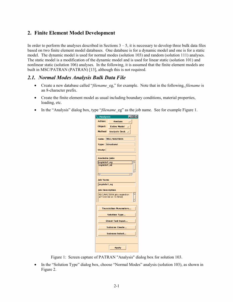
2.1. Normal Modes Analysis Bulk Data File • Create a new database called �filename_eg,� for example. Note that in the following, filename is

an 8-character prefix.

• Create the finite element model as usual including boundary conditions, material properties, loading, etc.

• In the �Analysis� dialog box, type �filename_eg� as the job name. See for example Figure 1.

Figure 1: Screen capture of PATRAN "Analysis" dialog box for solution 103.

• In the �Solution Type� dialog box, choose �Normal Modes� analysis (solution 103), as shown in Figure 2.

2-2

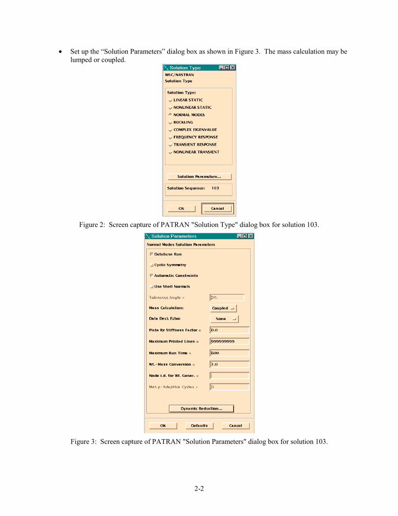
• Set up the �Solution Parameters� dialog box as shown in Figure 3. The mass calculation may be lumped or coupled.

Figure 2: Screen capture of PATRAN "Solution Type" dialog box for solution 103.

Figure 3: Screen capture of PATRAN "Solution Parameters" dialog box for solution 103.

2-3

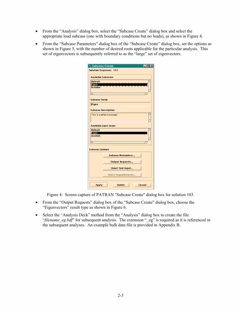
• From the �Analysis� dialog box, select the �Subcase Create� dialog box and select the appropriate load subcase (one with boundary conditions but no loads), as shown in Figure 4.

• From the �Subcase Parameters� dialog box of the �Subcase Create� dialog box, set the options as shown in Figure 5, with the number of desired roots applicable for the particular analysis. This set of eigenvectors is subsequently referred to as the �large� set of eigenvectors.

Figure 4: Screen capture of PATRAN "Subcase Create" dialog box for solution 103.

• From the �Output Requests� dialog box of the �Subcase Create� dialog box, choose the �Eigenvectors� result type as shown in Figure 6.

• Select the �Analysis Deck� method from the �Analysis� dialog box to create the file �filename_eg.bdf� for subsequent analysis. The extension �_eg� is required as it is referenced in the subsequent analyses. An example bulk data file is provided in Appendix B.

2-4

Figure 5: Screen capture of PATRAN "Subcase Parameters" dialog box for solution 103.

Figure 6: Screen capture of PATRAN "Output Requests" dialog box for solution 103.

2-5

2.2. Static Analysis Bulk Data File • Copy the dynamic database �filename_eg.db� to �filename_st.db,� for example. The 8-character

prefix filename must be the same as that used for the normal modes bulk data file.

• Open �filename_st.db� in PATRAN and make the following modifications:

o Add an extra grid point with a connecting beam or rod element. Note the added element must have a nonlinear capability and be connected to the structure at a fixed boundary. Equivalence the node where the new element is connected to the structure and, if necessary, renumber so that the node numbers of the main structure are the same as those for the normal modes analysis. In this manner, the extra grid point and element number will be greater than the highest grid point and element number of the original model.

o Create a new load case and delete any previously applied loads from the model. To the new load case, apply an arbitrary non-zero nodal force at the extra grid point.

o To the new load case, create a constraint displacement set, which sets all degrees of freedom to zero values except for those at the extra grid point.

Note that the necessity to introduce an extra element is an artifact of the solver implemented in NASTRAN solutions 101 (linear static) and 106 (nonlinear static). Specifically, these solutions can only solve the forward static problem, that is, these solutions solve for a set of displacements from a specified loading. In order to determine the nonlinear stiffness coefficients, it is necessary to solve linear and nonlinear inverse problems, which compute the forces due to a prescribed set of displacements. The extra element is introduced to allow NASTRAN to solve for a dummy set of displacements with the set of prescribed displacements acting as displacement constraints. The sought vector of applied loads (not including the extra load) is identical to the set of single-point-constraint forces in NASTRAN terminology.

Figure 7: Screen capture of PATRAN "Solution Parameters" dialog box for solution 106.

• In the �Analysis� dialog box, type �filename_st� as the job name.

2-6

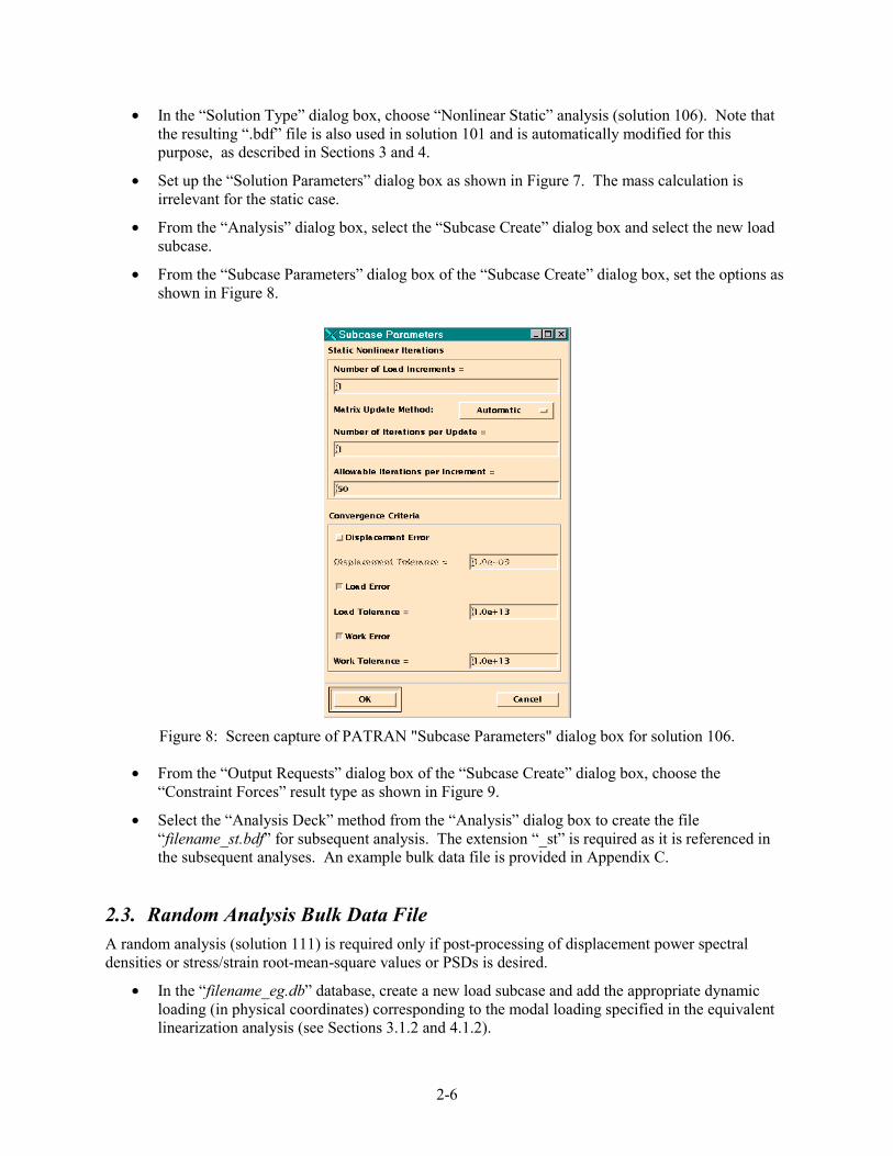
• In the �Solution Type� dialog box, choose �Nonlinear Static� analysis (solution 106). Note that the resulting �.bdf� file is also used in solution 101 and is automatically modified for this purpose, as described in Sections 3 and 4.

• Set up the �Solution Parameters� dialog box as shown in Figure 7. The mass calculation is irrelevant for the static case.

• From the �Analysis� dialog box, select the �Subcase Create� dialog box and select the new load subcase.

• From the �Subcase Parameters� dialog box of the �Subcase Create� dialog box, set the options as shown in Figure 8.

Figure 8: Screen capture of PATRAN "Subcase Parameters" dialog box for solution 106.

• From the �Output Requests� dialog box of the �Subcase Create� dialog box, choose the �Constraint Forces� result type as shown in Figure 9.

• Select the �Analysis Deck� method from the �Analysis� dialog box to create the file �filename_st.bdf� for subsequent analysis. The extension �_st� is required as it is referenced in the subsequent analyses. An example bulk data file is provided in Appendix C.

2.3. Random Analysis Bulk Data File A random analysis (solution 111) is required only if post-processing of displacement power spectral densities or stress/strain root-mean-square values or PSDs is desired.

• In the �filename_eg.db� database, create a new load subcase and add the appropriate dynamic loading (in physical coordinates) corresponding to the modal loading specified in the equivalent linearization analysis (see Sections 3.1.2 and 4.1.2).

2-7

Figure 9: Screen capture of PATRAN "Output Requests" dialog box for solution 106.

Figure 10: Screen capture of PATRAN "Solution Parameters" dialog box for solution 111.

2-8

• In the �Solution Type� dialog box, choose �Frequency Response� analysis.

• In the �Solution Parameters� dialog box, select the settings as indicated in Figure 10 with the formulation as modal to specify solution 111 and mass calculation as desired (lumped or coupled).

• Select the �Eigenvalue Extraction� dialog box from the �Solution Parameters� dialog box and set up the values as indicated in Figure 11. The number of desired roots should be the same as the large set of eigenvectors specified in the development of the normal modes analysis bulk data file.

Figure 11: Screen capture of PATRAN "Eigenvalue Extraction" dialog box for solution 111.

• From the �Subcase Create� dialog box, specify the frequency range in the �Subcase Parameters� dialog box. See Figure 12, for example. For consistent results between the equivalent linearization analysis and the solution 111 post-processing analysis, the frequency range should be the same as that used in the equivalent linearization analysis (see Sections 3.1.4 and 4.1.4).

Figure 12: Screen capture of PATRAN "Subcase Parameters" dialog box for solution 111.

• In the �Analysis� dialog box, type fixeD111_rd as the job name to create the bulk data file fixeD111_rd.bdf. This filename is required as it is referenced in the subsequent analysis.

• It is necessary to manually edit the bulk data file fixeD111_rd.bdf in preparation for the analysis run. The manual edits are indicated in bold in the sample listing provided in Appendix D.

3-1

3. FORTRAN Implementation

The analysis is subdivided into two parts. The first part calculates the nonlinear stiffness coefficients. The second part performs one of two equivalent linearization procedures to compute the total equivalent stiffness matrix and RMS displacements. A description of optional post-processing is provided in Section 5.

3.1. Input Files In addition to the bulk data files discussed in Section 2, several additional input files are required to specify various parameters used in the analysis. These are detailed below.

3.1.1. Modes Selection File

The file fixed.mod indicates which eigenvectors out of the large set of eigenvectors participate in the analysis. The format for fixed.mod is a free ASCII format as specified below.

LINE 1: Number of selected modes (NMOD).

LINE 2: Selected modes (e.g. 1st and 4th).

LINE 3: Scaling coefficients for each eigenvector selected. The product of each eigenvector and scaling coefficient produces a displacement field, which is used as a prescribed displacement set. The scaling coefficients should be chosen to be equal and not made too large so that the product of the eigenvector and coefficient will represent a realistic prescribed displacement within the linear range. The value of 1.0e-4 appears to work well for cases considered thus far.

A sample listing of fixed.mod with two selected modes (NMOD=2) is provided below. 2

1 4

1.e-04 1.e-04

Note that specification of the participating modes may necessitate running a standard normal modes analysis prior to the procedure for calculating the nonlinear stiffness coefficients described in Section 3.2. In addition, if a post-processing analysis is to be performed (as described in Section 5), the same information must also be specified in the file fixeD.mod, as described in Section 4.1.1.

3.1.2. Spectral Density Loads File

The file fixed.den contains the spectral density matrix of the applied loads in modal coordinates � � �ffS � . The format for fixed.den is a free ASCII format as specified below.

LINE 1: Number of breakpoints used to define frequency spectrum. (Min 2, Max 50). Between each breakpoint, each value of the � � �ffS � is linearly interpolated at the frequency increment specified in fixed.par (see Section 3.1.4).

LINE 2: Frequency of first breakpoint (Hz)

LINE 3: First row of modal spectral density matrix (NMOD entries) at first frequency breakpoint.

�

LINE 3 + NMOD: Last row of modal spectral density matrix (NMOD entries) at first frequency breakpoint

3-2

(Lines 2 to Line 3+NMOD are repeated for each breakpoint)

A sample listing of fixed.den for a flat spectrum between 0-1024 Hz with two selected modes is provided below.

2

0.00000000000000

6.83899171960566 2.27952175755947

2.27952175755446 0.759793205814123

1024.00000000000

6.83899171960566 2.27952175755947

2.27952175755446 0.759793205814123 To be explicit, at both 0 and 1024 Hz, the following spectral density matrix of applied loads in modal coordinates is specified:

� � �� �

� �

11 12

21 22

6.84 2.280,1024

2.28 0.76ff ff

ffff ff

S SS

S S

� � � �� �� � � �

� �� �� �

This matrix is computed as

� � � � �Tff ffS S� � � �� (1)

where � �ffS � is the fully-populated, real-valued spectral density matrix of the load in physical

coordinates and � is the subset of selected eigenvectors. Because � �ffS � is real-valued, only correlated inputs are permitted. This condition allows loadings such as normal acoustic pressure, inertial loading (for base excitation), and one or more correlated point forces or moments. It does not allow loadings which generate complex terms, such as grazing incidence acoustic loading.

The values of � �ffS � specify the double-sided spectrum level in units2/rad/sec. In order to specify the

same load in physical coordinates for a solution 111 post-processing analysis, the values of � �ffS � must be converted to a single-sided spectral density in units2/Hz by multiplying by 2 x 2π. These may then be specified on the TABRND1 card of the bulk data file.

From equation (1), it is obvious that a normal modes analysis must first be performed to obtain the eigenvectors. Several files containing eigenvectors are formed in the first part of the analysis used to calculate the nonlinear stiffness coefficients (see Section 3.2). The eigenvectors to be used in equation (1) are the set of selected g-size (all degrees of freedom including constrained ones) eigenvectors from the file egveCa.dat.

In order to facilitate generation of the modal spectral density matrix of the applied loading, the utility program gensff (described in Section 3.3) may be used to automatically compute the values and write them to fixed.den for a limited set of loading conditions.

3-3

3.1.3. Damping Matrix File

The file fixed.dam contains the diagonal modal damping matrix. The format for fixed.dam is a free ASCII formatted square matrix (NMOD × NMOD) as specified below.

1

2

0 00 0 0

0 NMOD

CC

C

� �� �� �� �� �� �� �

�

� �

A sample listing of fixed.dam with two selected modes is provided below.

14.6618 0.

0. 14.6618

In order to specify the same damping for a solution 111 post-processing analysis, the values must be converted to percent critical damping through the usual relation

2

ii

i

C�

��

where iC are the modal damping values (as specified in fixed.dam) and i� are the linear eigenvalues, not those of the equivalent linear system. This value of load may then be specified on the TABDMP1 card of the bulk data file.

3.1.4. Parameter File

The file fixed.par contains various additional parameters required for the analysis. The format for fixed.par is a free ASCII format as specified below.

LINE 1: Minimum and maximum frequency range of the analysis (Hz). Note that the maximum frequency range should be selected well beyond the frequency of the highest selected mode. This is necessary so that the resonant frequencies don�t shift out of the analysis bandwidth as nonlinearity increases. If the minimum or maximum analysis frequencies specified above fall outside of the bandwidth of applied loads (specified in fixed.den), the load will be padded with zeros at either low or high frequency end. If the minimum or maximum analysis frequencies fall inside of the bandwidth of applied loads, the loading will start and end at the frequencies specified above.

LINE 2: Frequency increment used in the analysis (Hz)

LINE 3: Weightings � and � . A discussion on how the weightings are used is given in [12]. The weightings must sum to 1. Typical initial values are 0.4� � and 0.6� � for the force error minimization approach and 0.05� � and 0.95� � for the strain energy error minimization approach. The choice of weightings may influence the solution to which the system converges, as discussed in Section 3.3.1.

LINE 4: Convergence criteria � A sample listing of fixed.par is provided below.

3-4

0. 1024.

0.25

0.4 0.6

0.005

3.2. Calculation of Nonlinear Stiffness Coefficients The method for calculating nonlinear stiffness coefficients is shown in the flowchart in Figure 13. Each operation is separated by a dashed line and is run in the sequence shown from top to bottom. The various operations are described below.

• prep103 � This FORTRAN program reads the bulk data file �filename_eg.bdf� and rewrites it to the file fixed103_eg.bdf. The program prep103 adds lines to the file management and case control sections of the bulk data file �filename_eg.bdf.� The lines that are added are shown in bold in Appendix E. It also creates the file prob_prefix.scr, which contains the 8-character prefix (i.e. filename) for use in other file manipulation programs.

• The first NASTRAN run calculates the eigenvectors of the model and writes them to two files for subsequent use as described below. This NASTRAN run utilizes the DMAP alter dm_103.v to modify the standard normal modes analysis (solution 103).

o egvec.dat contains the mass-normalized large set of g-size eigenvectors (all degrees of freedom including constrained ones) requested in the modeling phase (see Figure 5). This is an ASCII file with the INPUTT4 DMAP matrix input format [14].

o egveH.dat contains the mass-normalized large set of l-size eigenvectors (all unconstrained degrees of freedom) requested in the modeling phase. This is a binary file.

• gendisp � This FORTRAN program generates the displacements fields used in the subsequent solution 106 and 101 runs. The following files are created:

o egveCa.dat contains the mass-normalized selected set of g-size eigenvectors specified in the file fixed.mod. This data is a subset of egvec.dat. This is an ASCII file with the INPUTT4 DMAP matrix input format.

o displ.pr2 contains the number of unique combinations of two modes (IN) and the combinations of those modes used to prescribe the displacement fields imposed for the inverse problems. This is an ASCII file in free format.

o displ.pr3 contains the number of unique combinations of three modes (IC) and the combinations of those modes used to prescribe the displacement fields imposed for the inverse problems. This is an ASCII file in free format.

o dispL.inn are the prescribed displacement fields used for the linear inverse problem. This is an ASCII file with the INPUTT4 DMAP matrix input format.

o displ.inn are the prescribed displacement fields used for the nonlinear inverse problem. This is an ASCII file with the INPUTT4 DMAP matrix input format.

• prep106 � This FORTRAN program reads the bulk data file �filename_st.bdf� and rewrites it to the file fixed106_st.bdf. The program prep106 adds lines to the file management and case control sections of the bulk data file �filename_st.bdf.� In particular, it writes the number of sub-cases (i.e. the number of prescribed displacement fields) required in the subsequent NASTRAN run. The number of sub-cases depends on the number of modes selected (NMOD), number of unique combinations of two modes (IN) from the number of modes selected, and the number of

3-5

unique combinations of three modes (IC) from the number of modes selected. It is calculated using the following relation

2NSUBC NMOD+3 IN IC� � � �

Thus for NMOD = 3, IN = 3 (combinations of modes 1&2, 2&3, and 1&3), IC = 1 (combination of modes 1&2&3) and the number of sub-cases NSUBC = 16. As an example, a listing of the changed lines of file fixed106_st.bdf are shown in bold in Appendix F for NMOD = 2.

• The second NASTRAN run calculates the force vector corresponding to the prescribed displacement fields (provided in the file displ.inn) in a nonlinear analysis. Because it is not possible to separate the linear and nonlinear components, the resulting force vector contains the combined force. The resulting force vector is written to f_N.frc, an ASCII file with the INPUTT4 DMAP matrix input format. The DMAP alter dm_106.v is used to modify the standard nonlinear static analysis (solution 106).

• prep101 � This FORTRAN program reads the bulk data file �filename_st.bdf� and rewrites it to the file fixed101_st.bdf. The program prep101 adds lines to the file management and case control sections of the bulk data file �filename_st.bdf.� In particular, it writes the number of sub-cases (i.e. the number of prescribed displacement fields) required in the subsequent NASTRAN run. The number of sub-cases is equal to the number of modes selected (NMOD). As an example, a listing of the changed lines of file fixed101_st.bdf are shown in bold in Appendix G for NMOD = 2.

• The third NASTRAN run calculates the force vector corresponding to the prescribed displacement fields (provided in the file dispL.inn) in linear analysis. The resulting force vector is written to f1_L.frc, an ASCII file with the INPUTT4 DMAP matrix input format. The DMAP alter dm_101.v is used to modify the standard linear static analysis (solution 101).

• nlcfs � This FORTRAN program calculates the nonlinear stiffness coefficients of the structure and stores them in the file nlcfS.dat. Note that both quadratic jka and cubic jklb stiffness coefficients [10-12] are computed in nlcfs, but only the cubic terms are stored in nlcfS.dat because a zero mean response is assumed. The file nlcfS.dat is an ASCII file with the FORTRAN format (1P,3E23.16).

The nonlinear stiffness coefficients computed through this series of operations depend only on the structure (geometry, material properties, and boundary conditions) and not on the loading level or distribution. Therefore, this portion of the analysis only needs to be performed once for a given structural configuration. The effect of loading is addressed in the next sequence of analyses (see Section 3.3). In order to check the functioning of the entire analysis procedure, it is recommended that a linear analysis be run from this point forward using the two remaining sequences of analyses (see Sections 3.3 and 5) as is. To do so, all nonlinear stiffness coefficients in nlcfS.dat should be set to very small (non-zero) values (e.g. 10-15), and the weighting � and � in the file fixed.par should be set to 1 and 0, respectively. If everything is working well, the results obtained will be virtually identical to those from a linear solution 111 analysis. The UNIX script file doit1.bat (see Appendix A) runs the first part of the analysis as outlined above in an automated fashion. Some commands in doit1.bat may need to be modified depending on the operating system and how NASTRAN is installed. Removal (or transfer to another directory) of previously created ELSTEP output files is necessary for proper program execution. Removal of previously created standard NASTRAN files, e.g. *.f06, *.f04, *.op2, *.log, and *.pch, is optional, but helps to reduced clutter.

3-6

Figure 13: Flow-chart for calculation of nonlinear stiffness coefficients in the FORTRAN implementation.

prep103 filename_eg.bdf fixed103_eg.bdf

prob_prefix.scr

nastran fixed103_eg.bdf Solution 103

dm_103.v DMAP Alter

egvec.dat egveH.dat

gendisp fixed.mod egvec.dat

displ.pr2 displ.pr3 dispL.inn displ.inn

egveCa.dat

nastran fixed106_st.bdf Solution 106

dm_106.v DMAP Alter displ.inn f_N.frc

nastran fixed101_st.bdf Solution 101

dm_101.v DMAP Alter dispL.inn f1_L.frc

nlcfs nlcfS.dat fixed.mod egveCa.dat

displ.pr2 displ.pr3 f1_L.frc f_N.frc

prep106 filename_st.bdf displ.pr2 prob_prefix.scr displ.pr3

egveCa.dat fixed106_st.bdf

prep101 filename_st.bdf egveCa.dat prob_prefix.scr

fixed101_st.bdf

3-7

3.3. Equivalent Linearization Procedure

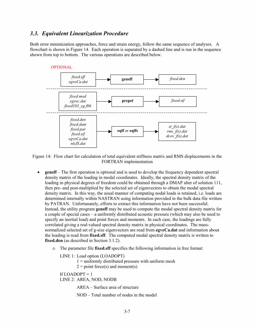
Both error minimization approaches, force and strain energy, follow the same sequence of analyses. A flowchart is shown in Figure 14. Each operation is separated by a dashed line and is run in the sequence shown from top to bottom. The various operations are described below.

Figure 14: Flow chart for calculation of total equivalent stiffness matrix and RMS displacements in the FORTRAN implementation

• gensff � The first operation is optional and is used to develop the frequency dependent spectral density matrix of the loading in modal coordinates. Ideally, the spectral density matrix of the loading in physical degrees of freedom could be obtained through a DMAP alter of solution 111, then pre- and post-multiplied by the selected set of eigenvectors to obtain the modal spectral density matrix. In this way, the usual manner of computing nodal loads is retained, i.e. loads are determined internally within NASTRAN using information provided in the bulk data file written by PATRAN. Unfortunately, efforts to extract this information have not been successful. Instead, the utility program gensff may be used to compute the modal spectral density matrix for a couple of special cases � a uniformly distributed acoustic pressure (which may also be used to specify an inertial load) and point forces and moments. In each case, the loadings are fully correlated giving a real-valued spectral density matrix in physical coordinates. The mass-normalized selected set of g-size eigenvectors are read from egveCa.dat and information about the loading is read from fixed.sff. The computed modal spectral density matrix is written to fixed.den (as described in Section 3.1.2).

o The parameter file fixed.sff specifies the following information in free format:

LINE 1: Load option (LOADOPT) 1 = uniformly distributed pressure with uniform mesh 2 = point force(s) and moment(s)

If LOADOPT = 1 LINE 2: AREA, NOD, NODB

AREA � Surface area of structure

NOD � Total number of nodes in the model

prepel fixed.mod egvec.dat

fixed103_eg.f06 fixed.stf

eqlf or eqlfs st_f(s).dat

rms_f(s).dat dcov_f(s).dat

fixed.den fixed.dam fixed.par fixed.stf

egveCa.dat nlcfS.dat

gensff fixed.sff egveCa.dat

fixed.den

OPTIONAL

3-8

NODB � Number of constrained (boundary) nodes

Forces at the grid points are obtained by multiplying the pressure level by the area and distributing these over the mesh, hence the need for a uniform mesh. If a non-uniform mesh is used, a pressure loading may be specified using LOADOPT = 2 with forces input at each grid point.

LINE 3: NPT

NPT � Number of breakpoints in the PSD ( 2 NPT 50� � )

LINE 4: (repeated NPT times): FREQ, PSD

FREQ, PSD � Breakpoint pairs for PSD definition of uniformly distributed pressure. Values of PSD will be linearly interpolated between breakpoint pairs at the frequency increment specified in fixed.par. FREQ is the frequency specified in Hz. PSD is the single-sided pressure PSD in units2/Hz and is the same as would be used on the TABRND1 card for a solution 111 analysis. Note that gensff converts the load internally to a double-sided value in units2/rad/sec.

Note that in this case of a uniformly distributed pressure on a uniformly distributed mesh, the forces for each grid point are identical and act in the z-direction. Hence, all non-zero auto- and cross-spectral density values in ffS are equal. Further, each column is identical. These properties speed the computation of ffS� .

If LOADOPT = 2 LINE 2: NLOAD

NLOAD � Number of fully correlated point forces and moments.

LINE 3: NPT

NPT � Number of breakpoints in the PSD ( 2 NPT 50� � )

(Lines 4-5 repeated NLOAD times)

LINE 4: NODF, DOF1-DOF6

NODF � Grid point at which point force is applied

DOF1-DOF6 � Multiplier for each of six degree-of-freedoms at each grid point. An arbitrarily oriented force or moment may be applied in this fashion.

LINE 5: (repeated NPT times): FREQ, PSDF

FREQ, PSDF � Breakpoint pairs for PSD definition of point forces. Values of PSDF will be linearly interpolated between breakpoint pairs at the frequency increment specified in fixed.par. FREQ is the frequency in Hz. PSDF is the single-sided force PSD in units2/Hz and is the same as would be used on the TABRND1 card for a solution 111 analysis. Note that gensff converts the load internally to a double-sided value in units2/rad/sec.

Note that in this case, the forces for each grid point are not identical. Therefore, the non-zero auto- and cross-spectral density values in ffS are unequal and each

column is not identical. These properties make the computation of ffS� more intensive.

3-9

Note that in general, the cross-spectral densities of the input loading are required to specify ffS . However, since both load options require fully correlated (in phase) loadings, the cross-spectral density (CSD) terms may be obtained from the auto-spectral density (PSD) from the following relationship:

� �� �ij i jCSD PSD PSD� �

This allows for the specification of only the PSD values, and not both the PSD and CSD values, as indicated above. Note that gensff as currently implemented only takes the positive square root. Therefore, the specified loadings must have the same direction. Failure to do so will result in an inconsistency in the sign of the diagonal and off-diagonal terms in ffS .

In the upcoming examples, the following may be helpful. The values specified above for the spectral density matrix of the loading in physical coordinates ( ffS ) may be determined from an RMS level for a particular bandwidth using the following relation

2

2 2

RMSBW

ffS�

�

�

where BW is the frequency bandwidth in Hz. For example, for an RMS acoustic pressure of 2048 Pa (160.21 dB) and 0-1024 Hz bandwidth, the double-sided value of ffS is 325.95 Pa2/rad/sec. The corresponding single-sided value, which should be used in fixed.sff, is 4096 Pa2/Hz.

The following is an example of fixed.sff for the uniformly distributed pressure indicated above: 1

0.0903224 609 96

0. 4096.

1024. 4096.

The following is an example of fixed.sff for point forces. The force at grid point 305 acts in the z-direction and linearly increases in magnitude from 0 to 5 N2/Hz over the bandwidth 0-512 Hz. A second force acts in the x-direction at grid point 220 with a constant magnitude of 2 N2/Hz over the frequency range of 0-512 Hz. 2

2

2

305 0.0 0.0 1.0 0.0 0.0 0.0

0. 0.0

512. 5.0

220 2.0 0.0 0.0 0.0 0.0 0.0

0. 1.0

3-10

512. 1.0

Note that when converting from a uniform pressure load specified by load option 1 to a force load specified by load option 2, the PSD values specified in option 1 must be multiplied by the area squared.

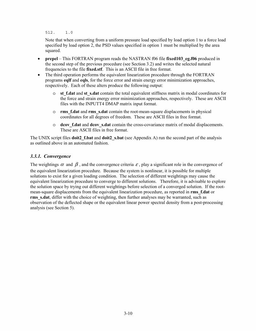
• prepel � This FORTRAN program reads the NASTRAN f06 file fixed103_eg.f06 produced in the second step of the previous procedure (see Section 3.2) and writes the selected natural frequencies to the file fixed.stf. This is an ASCII file in free format.

• The third operation performs the equivalent linearization procedure through the FORTRAN programs eqlf and eqls, for the force error and strain energy error minimization approaches, respectively. Each of these alters produce the following output:

o st_f.dat and st_s.dat contain the total equivalent stiffness matrix in modal coordinates for the force and strain energy error minimization approaches, respectively. These are ASCII files with the INPUTT4 DMAP matrix input format.

o rms_f.dat and rms_s.dat contain the root-mean-square displacements in physical coordinates for all degrees of freedom. These are ASCII files in free format.

o dcov_f.dat and dcov_s.dat contain the cross-covariance matrix of modal displacements. These are ASCII files in free format.

The UNIX script files doit2_f.bat and doit2_s.bat (see Appendix A) run the second part of the analysis as outlined above in an automated fashion.

3.3.1. Convergence The weightings � and � , and the convergence criteria � , play a significant role in the convergence of the equivalent linearization procedure. Because the system is nonlinear, it is possible for multiple solutions to exist for a given loading condition. The selection of different weightings may cause the equivalent linearization procedure to converge to different solutions. Therefore, it is advisable to explore the solution space by trying out different weightings before selection of a converged solution. If the root-mean-square displacements from the equivalent linearization procedure, as reported in rms_f.dat or rms_s.dat, differ with the choice of weighting, then further analyses may be warranted, such as observation of the deflected shape or the equivalent linear power spectral density from a post-processing analysis (see Section 5).

4-1

4. DMAP Implementation

As in the FORTRAN implementation, the analysis for the DMAP implementation is subdivided into two parts. The first part calculates the nonlinear stiffness coefficients. The second part performs one of two equivalent linearization procedures to compute the total equivalent stiffness matrix and RMS displacements. A description of optional post-processing is provided in Section 5. Note that since some files bear the same name but have a different format from those in the FORTRAN implementation, both FORTRAN and DMAP implementations should not be run from the same directory.

4.1. Input Files In addition to the bulk data files discussed in Section 2, several additional input files are required to specify various parameters used in the analysis. These are detailed below.

4.1.1. Modes Selection File

As in the FORTRAN implementation, the file fixeD.mod indicates which eigenvectors out of the large set of eigenvectors participate in the analysis. The format for fixeD.mod is a INPUTT4 DMAP matrix input format as specified below.

LINE 1: Number of columns (always 2), number of selected modes (NMOD), matrix form (always 2 for rectangular), type of matrix (always 2 for real, double precision), name of the matrix (always PHG), FORTRAN format specification (always 1P,3E23.16).

LINE 2: Column number (always 1), row position of first nonzero term (always 1), number of real double-precision entries on the following line (NMOD).

LINE 3: Selected modes (up to three per line). Note that these numbers are input as real and converted to integers within the program

LINE 4: Column number (always 2), row position of first nonzero term (always 1), number of real double-precision entries on the following line (NMOD).

LINE 5: Scaling coefficients for each eigenvector selected (up to three per line). See Section 3.1.1 for a discussion of these terms.

A sample listing of fixeD.mod with two selected modes (NMOD=2) is provided below.

2 2 2 2PHG 1P,3E23.16

1 1 2

1.0000000000000000E+00 4.0000000000000000E+00

2 1 2

1.0000000000000000E-04 1.0000000000000000E-04

It is clear that the size of this file depends on the number of modes selected. Since the format can be somewhat confusing, a sample listing with four selected modes (NMOD=4) is also provided below.

2 4 2 2PHG 1P,3E23.16

1 1 4

1.0000000000000000E+00 3.0000000000000000E+00 7.0000000000000000E+00

1.0000000000000000E+01

4-2

2 1 4

1.0000000000000000E-04 1.0000000000000000E-04 1.0000000000000000E-04

1.0000000000000000E-04

4.1.2. Spectral Density Loads File

The file fixeD.den is analogous to fixed.den in the FORTRAN implementation, except that the spectral density matrix of the applied loads in modal coordinates � ffS is independent of frequency in the DMAP implementation, i.e. only flat spectra may be applied. The format for fixeD.den is a INPUTT4 DMAP matrix input format as specified below.

LINE 1: Number of selected modes (NMOD), number of selected modes (NMOD), matrix form (always 1 for square), type of matrix (always 4 for complex, double precision), name of the matrix (always PHG), FORTRAN format specification (always 1P,6E13.6).

LINE 2: Column number (always 1), row position of first nonzero term (always 1), number of real double-precision entries on the following line (2 x NMOD).

LINE 3: First column of modal spectral density matrix (NMOD entries, up to 3 complex entries per line). Each entry is complex with the imaginary part equal to zero.

(Lines 2 and 3 repeat for NMOD selected modes)

2ND TO LAST LINE: Column number (always NMOD), row position of first nonzero term (always 1), number of real

double-precision entries on the following line (2 x NMOD).

LAST LINE: Last column of modal spectral density matrix (NMOD entries, up to 3 complex entries per line).

A sample listing of fixeD.den for two selected modes is provided below. 2 2 1 4PHG 1P,6E13.6

1 1 4

0.683899E+01 0.000000E+00 0.227952E+01 0.000000E+00

2 1 4

0.227952E+01 0.000000E+00 0.759793E+00 0.000000E+00

To be explicit, the above specifies the following frequency-independent spectral density matrix of applied loads in modal coordinates:

�� �

� �

� � � �

� � � �11 12

21 22

6.84,0 2.28,02.28,0 0.76,0

ff ffff

ff ff

S SS

S S

� � � �� �� � � �� � � �� �

This matrix is computed as

� Tff ffS S� �� (2)

where ffS is the real-valued spectral density matrix of the load in physical coordinates (double-sided spectrum level in units2/rad/sec) and � is the subset of selected eigenvectors. The eigenvectors to be used in equation (2) are the set of selected g-size (all degrees of freedom including constrained ones)

4-3

eigenvectors from the file egveCa.dat (see Section 4.2). As in the FORTRAN implementation, only correlated inputs are permitted. Values of ffS must be converted to single-sided values as indicated in Section 3.1.2 for use in a solution 111 post-processing analysis.

In order to facilitate generation of the modal spectral density matrix, the utility program gensffD (described in Section 4.3) may be used to automatically compute the values and write them to fixeD.den for a limited set of loading conditions.

4.1.3. Damping Matrix File

The file fixeD.dam is analogous to fixed.dam in the FORTRAN implementation. It contains the diagonal modal damping matrix. The format for fixeD.dam is a INPUTT4 DMAP matrix input format as specified below.

LINE 1: Number of selected modes (NMOD), number of selected modes (NMOD), matrix form (always 1 for square), type of matrix (always 2 for real, double precision), name of the matrix (always PHG), FORTRAN format specification (always 1P,3E23.16).

LINE 2: Row and column position of first modal damping values (always 1, 1), number of real double-precision entries on the following line (always 1).

LINE 3: First modal damping value

(Lines 2 and 3 repeat for NMOD selected modes)

2ND TO LAST LINE: Row and column position of last modal damping values (always NMOD, NMOD), number of

real double-precision entries on the following line (always 1).

LAST LINE: Last modal damping value. A sample listing of fixeD.dam with two selected modes is provided below.

2 2 1 2PHG 1P,3E23.16

1 1 1

0.1466180000000000E+02

2 2 1

0.1466180000000000E+02

In order to specify the same damping for a solution 111 post-processing analysis, the values must be converted to percent critical damping as discussed in Section 3.1.3.

4.1.4. Parameter File

The file fixeD.par is analogous to fixed.par in the FORTRAN implementation. It contains various additional parameters required for the analysis. The format for fixeD.par is a INPUTT4 DMAP matrix input format as specified below.

LINE 1: Number of columns (always 1), number of rows (always 6), matrix form (always 2 for rectangular), type of matrix (always 2 for real, double precision), name of the matrix (always PHG), FORTRAN format specification (always 1P,3E23.16).

LINE 2: Column number (always 1), row position of first nonzero term (always 1), number of real double-precision entries on the following line (always 6).

4-4

LINE 3: Minimum and maximum frequency range of the analysis (Hz), frequency increment used in the analysis (Hz). Note that the maximum frequency range should be selected well beyond the frequency of the highest selected mode. This is necessary so that the resonant frequencies don�t shift out of the analysis bandwidth as nonlinearity increases.

LINE 4: Weightings � and � , and convergence criteria � (see Section 3.1.4 for description). Note that these values are put on a fourth line because the format on line 1 indicates up to three values per line. The choice of weightings may influence the solution to which the system converges, as discussed in Section 3.3.1.

A sample listing of fixeD.par is provided below.

1 6 2 2PHG 1P,3E23.16

1 1 6

0.0000000000000000E+00 1.0240000000000000E+03 0.2500000000000000E+00

0.4000000000000000E+00 0.6000000000000000E+00 0.5000000000000000E-02

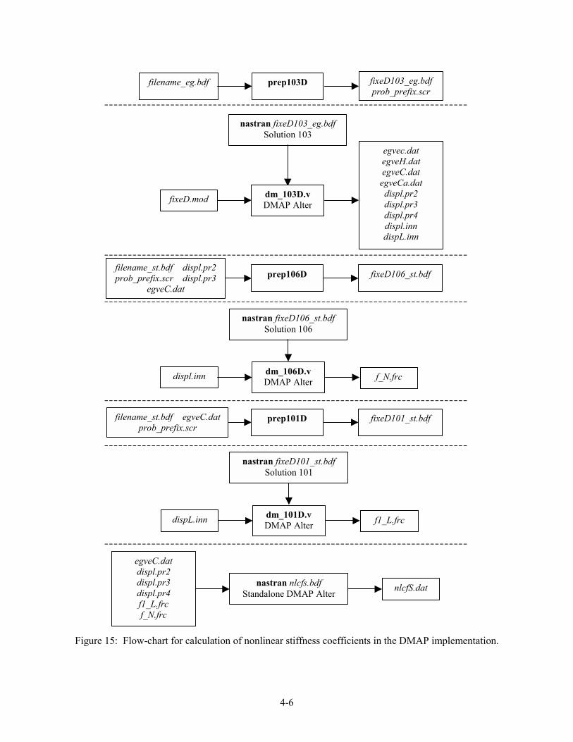
4.2. Calculation of Nonlinear Stiffness Coefficients The method of calculating the nonlinear stiffness coefficients is shown in the flowchart in Figure 15. Each operation is separated by a dashed line and is run in the sequence shown from top to bottom. The various operations are described below.

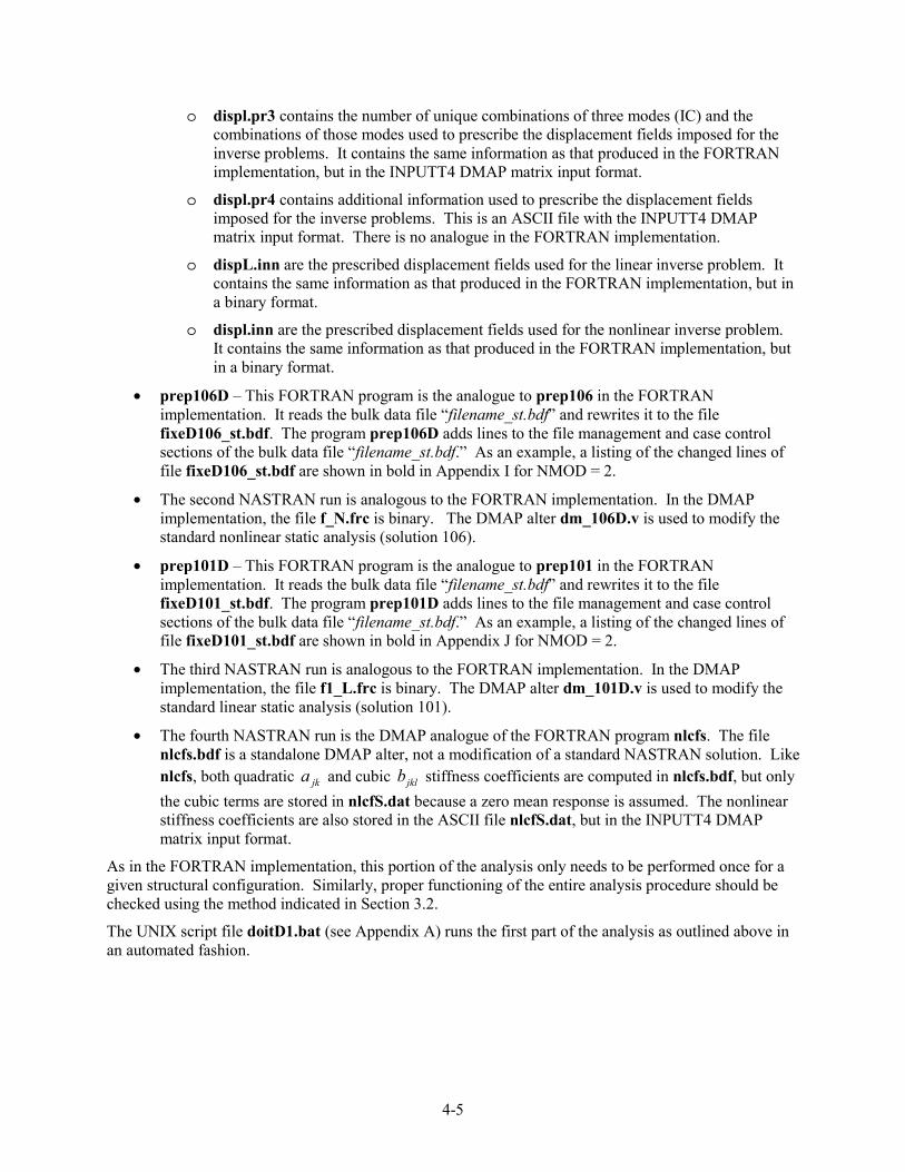
• prep103D � This FORTRAN program is the analogue to prep103 in the FORTRAN implementation. It reads the bulk data file �filename_eg.bdf� and rewrites it to the file fixeD103_eg.bdf. The program prep103D adds lines to the file management and case control sections of the bulk data file �filename_eg.bdf.� The lines that are added are shown in bold in Appendix H. It also creates the file prob_prefix.scr, which contains the 8-character prefix (i.e. filename) for use in other file manipulation programs.

• The first NASTRAN run is analogous to the FORTRAN implementation, except that the DMAP alter dm_103D.v also generates the displacement fields. These were generated by gendisp in the FORTRAN implementation. The following files are created:

o egvec.dat contains the mass-normalized large set of g-size eigenvectors (all degrees of freedom including constrained ones) requested in the modeling phase (see Figure 5). It contains the same information as that produced in the FORTRAN implementation, but in a binary format.

o egveH.dat contains the mass-normalized large set of l-size eigenvectors (all unconstrained degrees of freedom) requested in the modeling phase. This binary file is identical to that produced in the FORTRAN implementation.

o egveCa.dat contains the mass-normalized selected set of g-size eigenvectors specified in the file fixeD.mod. It is identical to that produced in the FORTRAN implementation.

o egveC.dat is a binary version of egveCa.dat. There is no analogue in the FORTRAN implementation.

o displ.pr2 contains the number of unique combinations of two modes (IN) and the combinations of those modes used to prescribe the displacement fields imposed for the inverse problems. It contains the same information as that produced in the FORTRAN implementation, but in the INPUTT4 DMAP matrix input format.

4-5

o displ.pr3 contains the number of unique combinations of three modes (IC) and the combinations of those modes used to prescribe the displacement fields imposed for the inverse problems. It contains the same information as that produced in the FORTRAN implementation, but in the INPUTT4 DMAP matrix input format.

o displ.pr4 contains additional information used to prescribe the displacement fields imposed for the inverse problems. This is an ASCII file with the INPUTT4 DMAP matrix input format. There is no analogue in the FORTRAN implementation.

o dispL.inn are the prescribed displacement fields used for the linear inverse problem. It contains the same information as that produced in the FORTRAN implementation, but in a binary format.

o displ.inn are the prescribed displacement fields used for the nonlinear inverse problem. It contains the same information as that produced in the FORTRAN implementation, but in a binary format.

• prep106D � This FORTRAN program is the analogue to prep106 in the FORTRAN implementation. It reads the bulk data file �filename_st.bdf� and rewrites it to the file fixeD106_st.bdf. The program prep106D adds lines to the file management and case control sections of the bulk data file �filename_st.bdf.� As an example, a listing of the changed lines of file fixeD106_st.bdf are shown in bold in Appendix I for NMOD = 2.

• The second NASTRAN run is analogous to the FORTRAN implementation. In the DMAP implementation, the file f_N.frc is binary. The DMAP alter dm_106D.v is used to modify the standard nonlinear static analysis (solution 106).

• prep101D � This FORTRAN program is the analogue to prep101 in the FORTRAN implementation. It reads the bulk data file �filename_st.bdf� and rewrites it to the file fixeD101_st.bdf. The program prep101D adds lines to the file management and case control sections of the bulk data file �filename_st.bdf.� As an example, a listing of the changed lines of file fixeD101_st.bdf are shown in bold in Appendix J for NMOD = 2.

• The third NASTRAN run is analogous to the FORTRAN implementation. In the DMAP implementation, the file f1_L.frc is binary. The DMAP alter dm_101D.v is used to modify the standard linear static analysis (solution 101).

• The fourth NASTRAN run is the DMAP analogue of the FORTRAN program nlcfs. The file nlcfs.bdf is a standalone DMAP alter, not a modification of a standard NASTRAN solution. Like nlcfs, both quadratic jka and cubic jklb stiffness coefficients are computed in nlcfs.bdf, but only the cubic terms are stored in nlcfS.dat because a zero mean response is assumed. The nonlinear stiffness coefficients are also stored in the ASCII file nlcfS.dat, but in the INPUTT4 DMAP matrix input format.

As in the FORTRAN implementation, this portion of the analysis only needs to be performed once for a given structural configuration. Similarly, proper functioning of the entire analysis procedure should be checked using the method indicated in Section 3.2.

The UNIX script file doitD1.bat (see Appendix A) runs the first part of the analysis as outlined above in an automated fashion.

4-6

Figure 15: Flow-chart for calculation of nonlinear stiffness coefficients in the DMAP implementation.

prep103D filename_eg.bdf fixeD103_eg.bdf

prob_prefix.scr

nastran fixeD103_eg.bdfSolution 103

dm_103D.v DMAP Alter fixeD.mod

egvec.dat egveH.dat egveC.dat

egveCa.dat displ.pr2 displ.pr3 displ.pr4 displ.inn dispL.inn

prep106D filename_st.bdf displ.pr2 prob_prefix.scr displ.pr3

egveC.dat fixeD106_st.bdf

nastran fixeD106_st.bdf Solution 106

dm_106D.v DMAP Alter displ.inn f_N.frc

prep101D filename_st.bdf egveC.dat prob_prefix.scr

fixeD101_st.bdf

nastran fixeD101_st.bdf Solution 101

dm_101D.v DMAP Alter dispL.inn f1_L.frc

nastran nlcfs.bdf Standalone DMAP Alter nlcfS.dat

egveC.dat displ.pr2 displ.pr3 displ.pr4 f1_L.frc f_N.frc

4-7

4.3. Equivalent Linearization Procedure Like the FORTRAN implementation, both force and strain energy error minimization approaches follow the same sequence of analyses, as shown in Figure 16. Each operation is separated by a dashed line and is run in the sequence shown from top to bottom. The various operations are described below.

Figure 16: Flow chart for calculation of total equivalent stiffness matrix and RMS displacements in the DMAP implementation.

• gensffD � The first operation is optional and is used to develop the spectral density matrix of the loading in modal coordinates. It is analogous to the program gensff in the FORTRAN implementation, except that in the DMAP implementation, the spectral density matrices are independent of frequency, i.e. only flat spectra may be specified. The program gensffD may be used to compute the modal spectral density matrix for a couple of special cases � a uniformly distributed acoustic pressure (which may also be used to specify an inertial load) and point forces and moments. In each case, the loadings are fully correlated giving a real-valued spectral density matrix in physical coordinates. The mass-normalized selected set of g-size eigenvectors are read from egveCa.dat and information about the loading is read from fixeD.sff. The computed modal spectral density matrix is written to fixeD.den (as described in Section 4.1.2).

o The parameter file fixeD.sff specifies the following information in free format:

LINE 1: Load option (LOADOPT) 1 = uniformly distributed pressure with uniform mesh 2 = point force(s) and moment(s)

If LOADOPT = 1 LINE 2: PSD, AREA, NOD, NODB

prepelD fixeD.mod egvec.dat

fixeD103_eg.f06 fixeD.stf

nastran eql_f(s).bdf Standalone DMAP Alter

st_f(s).dat rms_f(s).dat dcov_f(s).dat

postelfD or postelsD

rms_f(s).dat rms_f(s)R.nod rms_f(s).nod

fixeD.mod fixeD.den fixeD.dam fixeD.par fixeD.stf

egveC.dat nlcfS.dat

OPTIONAL

gensffD fixeD.sff egveCa.dat

fixeD.den

OPTIONAL

4-8

PSD � Spectrum level of uniformly distributed pressure in units2/Hz. This level is a single-sided value and is the same as would be used on the TABRND1 card for sol 111 analysis. Note that gensffD converts the load internally to a double-sided value in units2/rad/sec.

AREA � Surface area of structure

NOD � Total number of nodes in the model

NODB � Number of constrained (boundary) nodes

Forces at the grid points are obtained by multiplying the pressure level by the area and distributing these over the mesh, hence the need for a uniform mesh. If a non-uniform mesh is used, a pressure loading may be specified using LOADOPT = 2 with forces input at each grid point.

Note that in this case of a uniformly distributed pressure on a uniformly distributed mesh, the forces for each grid point are identical and act in the z-direction. Hence, all non-zero auto- and cross-spectral density values in ffS are equal. Further, each column is identical. These properties speed the computation of ffS� .

If LOADOPT = 2 LINE 2: NLOAD

NLOAD � Number of fully correlated point forces and moments.

LINE 3 (repeated NLOAD times): NODF, PSDF, DOF1-DOF6

NODF � Grid point at which point force is applied

PSDF � Spectrum level of force in units2/Hz. This level is a single-sided value and is the same as would be used on the TABRND1 card for sol 111 analysis. Note that gensffD converts the load internally to a double-sided value in units2/rad/sec.

DOF1-DOF6 � Multiplier for each of six degree-of-freedoms at each grid point. An arbitrarily oriented force or moment may be applied in this fashion.

Note that in this case, the forces for each grid point are not identical. Therefore, the non-zero auto- and cross-spectral density values in ffS are unequal and each

column is not identical. These properties make the computation of ffS� more intensive.

Note that in general, the cross-spectral densities of the input loading are required to specify ffS . However, since both load options require fully correlated (in phase) loadings, the cross-spectral density (CSD) terms may be obtained from the auto-spectral density (PSD) from the following relationship:

� �� �ij i jCSD PSD PSD� �

This allows for the specification of only the PSD values, and not both the PSD and CSD values, as indicated above. Note that gensffD as currently implemented only takes the positive square root. Therefore, the specified loadings must have the same direction.

4-9

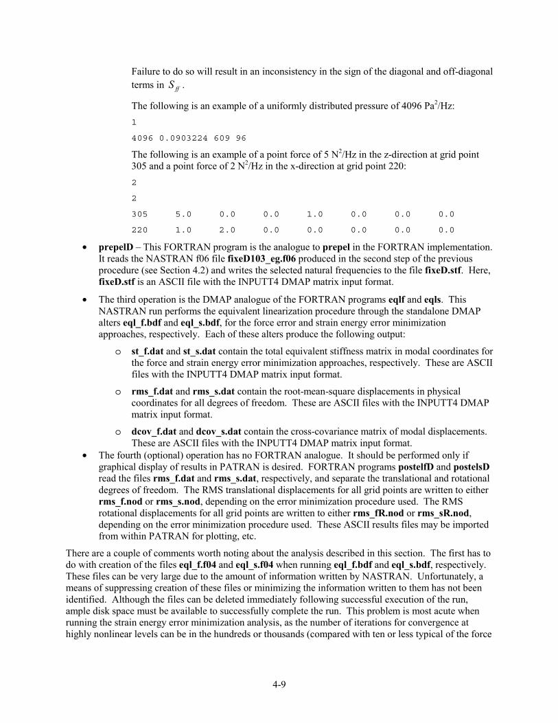
Failure to do so will result in an inconsistency in the sign of the diagonal and off-diagonal terms in ffS .

The following is an example of a uniformly distributed pressure of 4096 Pa2/Hz: 1

4096 0.0903224 609 96

The following is an example of a point force of 5 N2/Hz in the z-direction at grid point 305 and a point force of 2 N2/Hz in the x-direction at grid point 220: 2

2

305 5.0 0.0 0.0 1.0 0.0 0.0 0.0

220 1.0 2.0 0.0 0.0 0.0 0.0 0.0

• prepelD � This FORTRAN program is the analogue to prepel in the FORTRAN implementation. It reads the NASTRAN f06 file fixeD103_eg.f06 produced in the second step of the previous procedure (see Section 4.2) and writes the selected natural frequencies to the file fixeD.stf. Here, fixeD.stf is an ASCII file with the INPUTT4 DMAP matrix input format.

• The third operation is the DMAP analogue of the FORTRAN programs eqlf and eqls. This NASTRAN run performs the equivalent linearization procedure through the standalone DMAP alters eql_f.bdf and eql_s.bdf, for the force error and strain energy error minimization approaches, respectively. Each of these alters produce the following output:

o st_f.dat and st_s.dat contain the total equivalent stiffness matrix in modal coordinates for the force and strain energy error minimization approaches, respectively. These are ASCII files with the INPUTT4 DMAP matrix input format.

o rms_f.dat and rms_s.dat contain the root-mean-square displacements in physical coordinates for all degrees of freedom. These are ASCII files with the INPUTT4 DMAP matrix input format.

o dcov_f.dat and dcov_s.dat contain the cross-covariance matrix of modal displacements. These are ASCII files with the INPUTT4 DMAP matrix input format.

• The fourth (optional) operation has no FORTRAN analogue. It should be performed only if graphical display of results in PATRAN is desired. FORTRAN programs postelfD and postelsD read the files rms_f.dat and rms_s.dat, respectively, and separate the translational and rotational degrees of freedom. The RMS translational displacements for all grid points are written to either rms_f.nod or rms_s.nod, depending on the error minimization procedure used. The RMS rotational displacements for all grid points are written to either rms_fR.nod or rms_sR.nod, depending on the error minimization procedure used. These ASCII results files may be imported from within PATRAN for plotting, etc.

There are a couple of comments worth noting about the analysis described in this section. The first has to do with creation of the files eql_f.f04 and eql_s.f04 when running eql_f.bdf and eql_s.bdf, respectively. These files can be very large due to the amount of information written by NASTRAN. Unfortunately, a means of suppressing creation of these files or minimizing the information written to them has not been identified. Although the files can be deleted immediately following successful execution of the run, ample disk space must be available to successfully complete the run. This problem is most acute when running the strain energy error minimization analysis, as the number of iterations for convergence at highly nonlinear levels can be in the hundreds or thousands (compared with ten or less typical of the force

4-10

error minimization approach). Consequently, large temporary disk space is recommended when running the strain energy error minimization analysis.

The second item worth mentioning relates to the calculation of RMS displacements in physical coordinates when running eql_f.bdf and eql_s.bdf. Following calculation of the total equivalent stiffness matrix and cross-covariance matrix in modal coordinates, the RMS displacements in physical coordinates are recovered and stored in the files rms_f.dat and rms_s.dat. This process can take a significant amount of time as presently implemented due to the amount of disk I/O that occurs, especially for large models. If the intention is to perform a post-processing analysis to determine displacement PSDs and/or stress/strain information, as outlined in Section 5, a more efficient means of getting RMS displacements in physical coordinates is to request this information as part of that analysis. In this case, the value of RMSDISP should be changed from 1 to 0 in eql_f.bdf and eql_s.bdf to suppress computation of this data.

The UNIX script files doitD2_f.bat and doitD2_s.bat (see Appendix A) run the second part of the analysis as outlined above in an automated fashion.

4.3.1. Convergence The reader should refer to Section 3.3.1 for a discussion on convergence of the equivalent linearization procedure.

5-1

5. Post-Processing for Displacement, Stress and Strain PSDs

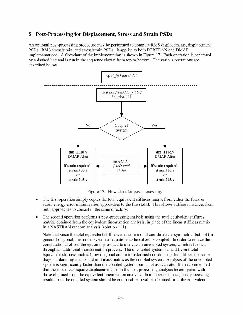
An optional post-processing procedure may be performed to compute RMS displacements, displacement PSDs , RMS stress/strain, and stress/strain PSDs. It applies to both FORTRAN and DMAP implementations. A flowchart of the implementation is shown in Figure 17. Each operation is separated by a dashed line and is run in the sequence shown from top to bottom. The various operations are described below.

Figure 17: Flow chart for post-processing.

• The first operation simply copies the total equivalent stiffness matrix from either the force or strain energy error minimization approaches to the file st.dat. This allows stiffness matrices from both approaches to coexist in the same directory.

• The second operation performs a post-processing analysis using the total equivalent stiffness matrix, obtained from the equivalent linearization analysis, in place of the linear stiffness matrix in a NASTRAN random analysis (solution 111).

Note that since the total equivalent stiffness matrix in modal coordinates is symmetric, but not (in general) diagonal, the modal system of equations to be solved is coupled. In order to reduce the computational effort, the option is provided to analyze an uncoupled system, which is formed through an additional transformation process. The uncoupled system has a different total equivalent stiffness matrix (now diagonal and in transformed coordinates), but utilizes the same diagonal damping matrix and unit mass matrix as the coupled system. Analysis of the uncoupled system is significantly faster than the coupled system, but is not as accurate. It is recommended that the root-mean-square displacements from the post-processing analysis be compared with those obtained from the equivalent linearization analysis. In all circumstances, post-processing results from the coupled system should be comparable to values obtained from the equivalent

cp st_f(s).dat st.dat

nastran fixeD111_rd.bdfSolution 111

egveH.dat fixeD.mod

st.dat

dm_111c.v DMAP Alter

If strain required -

strain700.v or

strain705.v

Coupled System

YesNo

dm_111u.v DMAP Alter

If strain required -

strain700.v or

strain705.v

5-2

linearization analysis. Only small differences, on the order of a few percent, should be found (see Section 6.4 for example), since the loading is specified equivalently but differently between the equivalent linearization and post-processing analyses. Post-processing results from the uncoupled system may or may not be comparable to values obtained from the equivalent linearization analysis. Thus, if results from the uncoupled analysis significantly differ from results from the equivalent linearization analysis, it is recommended that the coupled system be used for post-processing. The choice of coupled versus uncoupled system is made in the file fixeD111_rd.bdf (see Appendix D), through selection of the appropriate DMAP alter as shown in Figure 17.

If root-mean-square strain results are to be recovered, the alters strain700.v or strain705.v should be utilized. For NASTRAN version 70.0, the alter strain700.v should be used. For NASTRAN versions 70.5 and 70.7, the alter strain705.v should be used. If root-mean-square stress results are to be recovered, neither alter should be utilized. The choice of which alter to use (if any) is made in the file fixeD111_rd.bdf (see Appendix D). The file Strain-Recovery-Notes.pdf (see Appendix A) documents other commands required in the case control section for the different NASTRAN versions. Note that stress and strain results are recovered using linear strain/displacement relationships. This approach appears to be acceptable for the beam and plate analyses conducted to date.

Because the post-processing analysis is performed on the equivalent linear system, all PSDs appear linear in character. In other words, at nonlinear response levels, the PSDs exhibit neither peak broadening nor the same shifts in resonant frequencies as the truly nonlinear system.

Shifted resonant frequencies of the equivalent linear system are not directly reported since a modified solution 103, using the total equivalent stiffness matrix in place of the linear stiffness matrix, is not presently available. The shifted resonant frequencies may be determined by scanning the punch file fixeD111_rd.pch for peaks in the displacement PSD (when flat spectra are applied). Note that it may be necessary to run the post-processing analysis more than once so that the frequency ranges specified on the TABDMP1 card are centered about the shifted peaks of the equivalent linear system. The frequency range for each critical damping value is typically set to bracket the corresponding resonant peak at mid-span. As indicated in Section 3.1.3, the relationship between percent critical damping and modal damping values should remain based on the linear eigenvalues.

The UNIX script files doitD3_f.bat and doitD3_s.bat (see Appendix A) run the post-processing part of the analysis as outlined above in an automated fashion.

6-1

6. Example Problem

A simply support aluminum plate under normal acoustic excitation was chosen to illustrate the execution of ELSTEP and to generate sample results which may be used subsequently to verify proper execution with future NASTRAN and PATRAN releases. Consequently, many results are reported to a large number of significant digits.

The rectangular plate chosen measured 0.254m x 0.3556m x 0.00102m. All sides were simply supported. Material properties were:

10

3

7.3 10 Pa0.32763 kg/m

E�

�

� �

�

�

giving a flexural rigidity of

3 2

2 2

kg-m7.094 12(1 ) s

EhD�

� �

�

Natural frequencies may be computed from the following relation [15]

2 2

mnD m n

a b� �

��

� �� � � �� �� � � � � �� � �

giving

11

13

58.34 Hz216.01 Hz

�

�

�

�

for the first two symmetric modes.

A finite element model of this structure was built in PATRAN having 560 CQUAD4 elements measuring 0.0127m square. The first two symmetric modes (modes 1 and 4) of this model had natural frequencies of 58.38 and 217.27 Hz. These two modes were selected as participating modes in the ELSTEP analysis as per the example files in Sections 3.1.1 and 4.1.1. Modal damping was specified as per the example in Sections 3.1.3 and 4.1.3, giving percent critical damping values of 2% and 0.54% for modes 1 and 4, respectively.

A spatially uniform distributed normal acoustic pressure with RMS value of 2048 Pa, and a single-sided spectrum level of 4096 Pa2/Hz over a 0-1024 Hz bandwidth was applied to the plate. Using the example input file for a uniformly distributed pressure (described in Sections 3.3 and 4.3) for the programs gensff and gensffD, the modal spectral density matrix generated is as shown in Sections 3.1.2 and 4.1.2. Note that this load level gives rise to a highly nonlinear response.

6.1. Nonlinear Stiffness Results The cubic nonlinear stiffness coefficients were computed and written to nlcfS.dat. For the FORTRAN implementation, nlcfS.dat is written as:

4.1355686358055371E+12-1.6827938202459033E+12

2.3630088637711590E+13

4.0490613582441501E+07

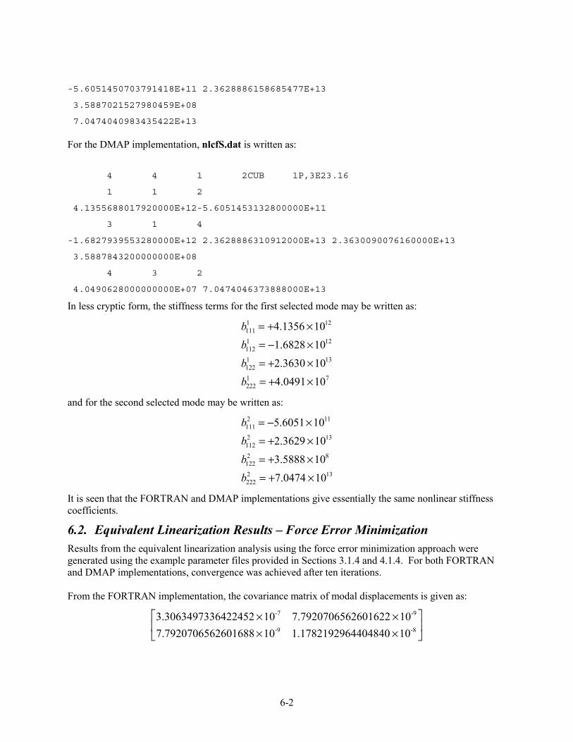
6-2

-5.6051450703791418E+11 2.3628886158685477E+13

3.5887021527980459E+08

7.0474040983435422E+13 For the DMAP implementation, nlcfS.dat is written as:

4 4 1 2CUB 1P,3E23.16

1 1 2

4.1355688017920000E+12-5.6051453132800000E+11

3 1 4

-1.6827939553280000E+12 2.3628886310912000E+13 2.3630090076160000E+13

3.5887843200000000E+08

4 3 2

4.0490628000000000E+07 7.0474046373888000E+13

In less cryptic form, the stiffness terms for the first selected mode may be written as:

1 121111 121121 131221 7222

4.1356 101.6828 102.3630 104.0491 10

bbbb

� � �

� � �

� � �

� � �

and for the second selected mode may be written as:

2 111112 131122 81222 13222

5.6051 102.3629 103.5888 107.0474 10

bbbb

� � �

� � �

� � �

� � �

It is seen that the FORTRAN and DMAP implementations give essentially the same nonlinear stiffness coefficients.

6.2. Equivalent Linearization Results � Force Error Minimization Results from the equivalent linearization analysis using the force error minimization approach were generated using the example parameter files provided in Sections 3.1.4 and 4.1.4. For both FORTRAN and DMAP implementations, convergence was achieved after ten iterations. From the FORTRAN implementation, the covariance matrix of modal displacements is given as:

-7 -9

-9 -8

3.3063497336422452 10 7.7920706562601622 107.7920706562601688 10 1.1782192964404840 10� �� �� �

� �� �

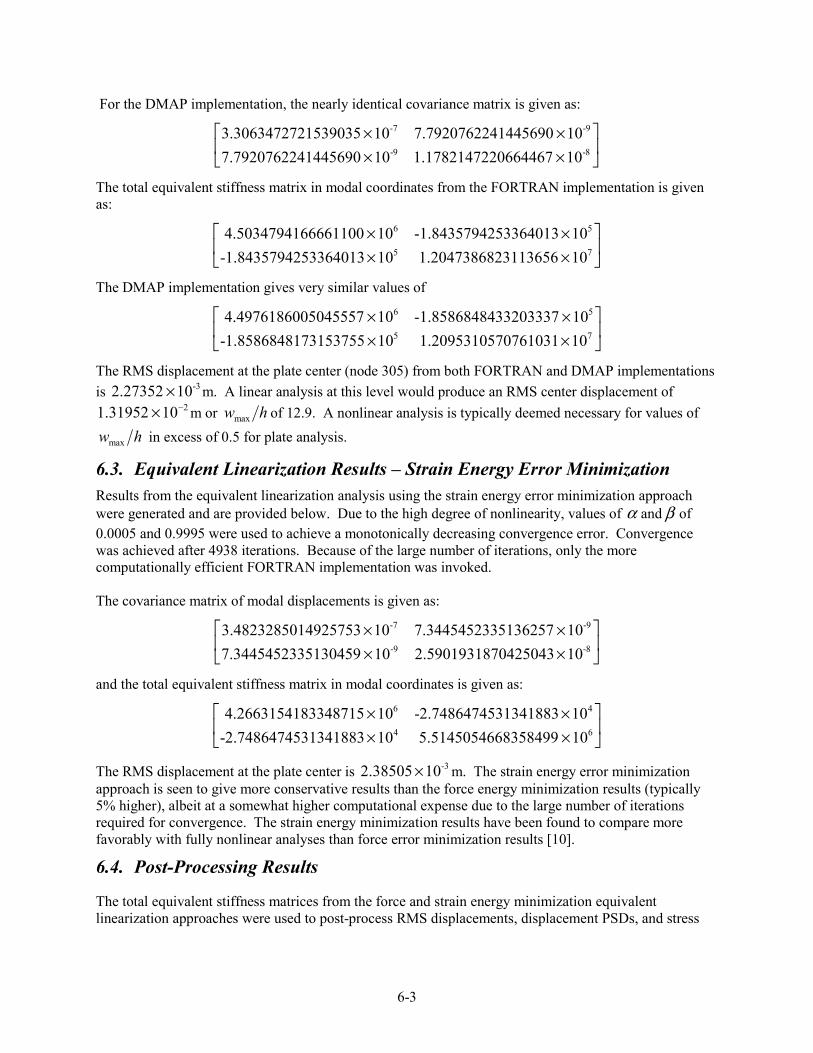
6-3

For the DMAP implementation, the nearly identical covariance matrix is given as:

-7 -9

-9 -8

3.3063472721539035 10 7.7920762241445690 107.7920762241445690 10 1.1782147220664467 10� �� �� �

� �� �

The total equivalent stiffness matrix in modal coordinates from the FORTRAN implementation is given as:

6 5

5 7

4.5034794166661100 10 -1.8435794253364013 10-1.8435794253364013 10 1.2047386823113656 10� �� �� �

� �� �

The DMAP implementation gives very similar values of

6 5

5 7

4.4976186005045557 10 -1.8586848433203337 10-1.8586848173153755 10 1.2095310570761031 10� �� �� �

� �� �

The RMS displacement at the plate center (node 305) from both FORTRAN and DMAP implementations is -32.27352 10� m. A linear analysis at this level would produce an RMS center displacement of

21.31952 10�

� m or maxw h of 12.9. A nonlinear analysis is typically deemed necessary for values of

maxw h in excess of 0.5 for plate analysis.

6.3. Equivalent Linearization Results � Strain Energy Error Minimization Results from the equivalent linearization analysis using the strain energy error minimization approach were generated and are provided below. Due to the high degree of nonlinearity, values of � and � of 0.0005 and 0.9995 were used to achieve a monotonically decreasing convergence error. Convergence was achieved after 4938 iterations. Because of the large number of iterations, only the more computationally efficient FORTRAN implementation was invoked. The covariance matrix of modal displacements is given as:

-7 -9

-9 -8

3.4823285014925753 10 7.3445452335136257 107.3445452335130459 10 2.5901931870425043 10� �� �� �

� �� �

and the total equivalent stiffness matrix in modal coordinates is given as:

6 4

4 6

4.2663154183348715 10 -2.7486474531341883 10-2.7486474531341883 10 5.5145054668358499 10� �� �� �

� �� �

The RMS displacement at the plate center is -32.38505 10� m. The strain energy error minimization approach is seen to give more conservative results than the force energy minimization results (typically 5% higher), albeit at a somewhat higher computational expense due to the large number of iterations required for convergence. The strain energy minimization results have been found to compare more favorably with fully nonlinear analyses than force error minimization results [10].

6.4. Post-Processing Results

The total equivalent stiffness matrices from the force and strain energy minimization equivalent linearization approaches were used to post-process RMS displacements, displacement PSDs, and stress

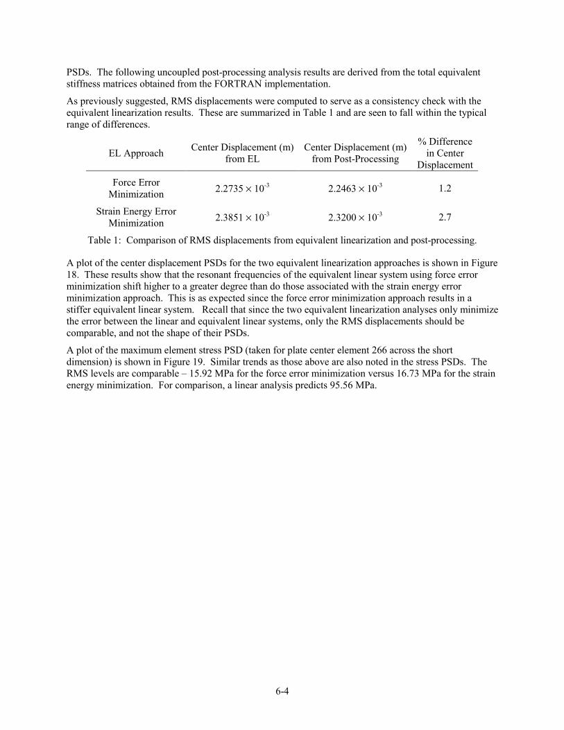
6-4

PSDs. The following uncoupled post-processing analysis results are derived from the total equivalent stiffness matrices obtained from the FORTRAN implementation.

As previously suggested, RMS displacements were computed to serve as a consistency check with the equivalent linearization results. These are summarized in Table 1 and are seen to fall within the typical range of differences.

EL Approach Center Displacement (m) from EL

Center Displacement (m) from Post-Processing

% Difference in Center

Displacement

Force Error Minimization 2.2735 × 10-3 2.2463 × 10-3 1.2

Strain Energy Error Minimization 2.3851 × 10-3 2.3200 × 10-3 2.7

Table 1: Comparison of RMS displacements from equivalent linearization and post-processing.

A plot of the center displacement PSDs for the two equivalent linearization approaches is shown in Figure 18. These results show that the resonant frequencies of the equivalent linear system using force error minimization shift higher to a greater degree than do those associated with the strain energy error minimization approach. This is as expected since the force error minimization approach results in a stiffer equivalent linear system. Recall that since the two equivalent linearization analyses only minimize the error between the linear and equivalent linear systems, only the RMS displacements should be comparable, and not the shape of their PSDs.

A plot of the maximum element stress PSD (taken for plate center element 266 across the short dimension) is shown in Figure 19. Similar trends as those above are also noted in the stress PSDs. The RMS levels are comparable � 15.92 MPa for the force error minimization versus 16.73 MPa for the strain energy minimization. For comparison, a linear analysis predicts 95.56 MPa.

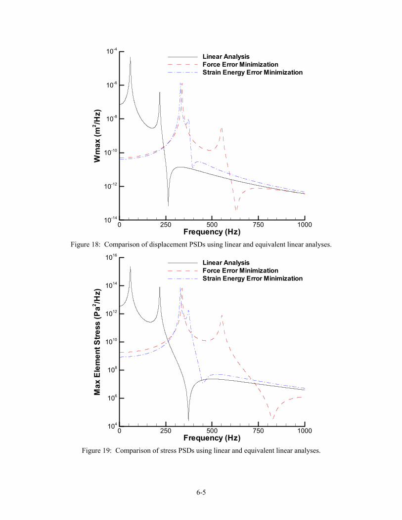
6-5

Figure 18: Comparison of displacement PSDs using linear and equivalent linear analyses.

Figure 19: Comparison of stress PSDs using linear and equivalent linear analyses.

Frequency (Hz)

Wmax(m

2 /Hz)

0 250 500 750 100010-14

10-12

10-10

10-8

10-6

10-4Linear AnalysisForce Error MinimizationStrain Energy Error Minimization

Frequency (Hz)

MaxElementStress(Pa2/Hz)

0 250 500 750 1000104

106

108

1010

1012

1014

1016Linear AnalysisForce Error MinimizationStrain Energy Error Minimization

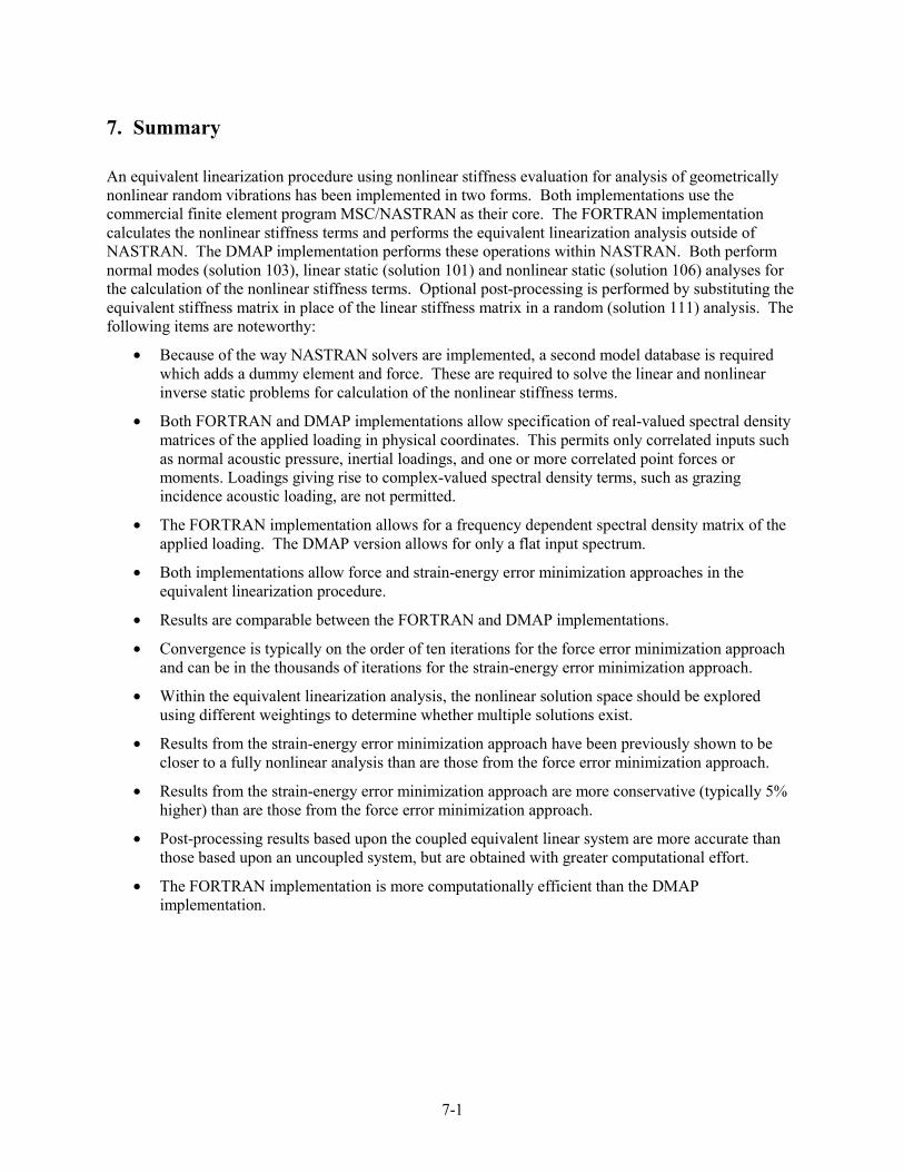
7-1

7. Summary

An equivalent linearization procedure using nonlinear stiffness evaluation for analysis of geometrically nonlinear random vibrations has been implemented in two forms. Both implementations use the commercial finite element program MSC/NASTRAN as their core. The FORTRAN implementation calculates the nonlinear stiffness terms and performs the equivalent linearization analysis outside of NASTRAN. The DMAP implementation performs these operations within NASTRAN. Both perform normal modes (solution 103), linear static (solution 101) and nonlinear static (solution 106) analyses for the calculation of the nonlinear stiffness terms. Optional post-processing is performed by substituting the equivalent stiffness matrix in place of the linear stiffness matrix in a random (solution 111) analysis. The following items are noteworthy:

• Because of the way NASTRAN solvers are implemented, a second model database is required which adds a dummy element and force. These are required to solve the linear and nonlinear inverse static problems for calculation of the nonlinear stiffness terms.

• Both FORTRAN and DMAP implementations allow specification of real-valued spectral density matrices of the applied loading in physical coordinates. This permits only correlated inputs such as normal acoustic pressure, inertial loadings, and one or more correlated point forces or moments. Loadings giving rise to complex-valued spectral density terms, such as grazing incidence acoustic loading, are not permitted.

• The FORTRAN implementation allows for a frequency dependent spectral density matrix of the applied loading. The DMAP version allows for only a flat input spectrum.

• Both implementations allow force and strain-energy error minimization approaches in the equivalent linearization procedure.

• Results are comparable between the FORTRAN and DMAP implementations.

• Convergence is typically on the order of ten iterations for the force error minimization approach and can be in the thousands of iterations for the strain-energy error minimization approach.

• Within the equivalent linearization analysis, the nonlinear solution space should be explored using different weightings to determine whether multiple solutions exist.

• Results from the strain-energy error minimization approach have been previously shown to be closer to a fully nonlinear analysis than are those from the force error minimization approach.

• Results from the strain-energy error minimization approach are more conservative (typically 5% higher) than are those from the force error minimization approach.

• Post-processing results based upon the coupled equivalent linear system are more accurate than those based upon an uncoupled system, but are obtained with greater computational effort.

• The FORTRAN implementation is more computationally efficient than the DMAP implementation.

8-1

8. References

[1] Bolotin, V.V., Statistical methods in structural mechanics, Holden-Day, Inc., 1969.

[2] Lin, Y.K., Probabilistic theory of structural dynamics. Malabar, FL, R.E. Krieger, 1976.

[3] Roberts, J.B. and Spanos, P.D., Random vibration and statistical linearization. New York, NY, John Wiley & Sons, 1990.

[4] Atalik, T.S. and Utku, S., "Stochastic linearization of multi-degree-of-freedom nonlinear systems," Earthquake engineering and structural dynamics, Vol. 4, pp. 411-420, 1976.

[5] Elishakoff, I. and Zhang, R., "Comparison of new energy-based versions of the stochastic linearization technique," IUTAM Symposium, Springer-Verlag, pp. 201-211, Turin, 1992.

[6] Zhang, X., Elishakoff, I., and Zhang, R., "A stochastic linearization technique based on minimum mean square deviation of potential energy," In Stochastic structural dynamics, Lin, Y.K. and Elishakoff, I., Eds., Springer-Verlag, pp. 328-338, 1991.

[7] "MSC/NASTRAN Quick Reference Guide, Version 70.5," MacNeal Schwendler Corporation, 1998.

[8] Robinson, J.H., Chiang, C.K., and Rizzi, S.A., "Nonlinear Random Response Prediction Using MSC/NASTRAN," NASA TM-109029, October 1993.

[9] Chiang, C.K., Robinson, J.H., and Rizzi, S.A., "An Equivalent Linearization Solution Sequence for MSC/NASTRAN," Symposium on Nonlinear Vibrations, ASME Winter Annual Meeting, Vol. DE-50, AMD-144, pp. 133-138, Anaheim, CA, 1992.

[10] Muravyov, A.A., Turner, T.L., Robinson, J.H., and Rizzi, S.A., "A New Stochastic Equivalent Linearization Implementation for Prediction of Geometrically Nonlinear Vibrations," Proceedings of the 40th AIAA/ASME/ASCE/AHS/ASC Structures, Structural Dynamics and Materials Conference, Vol. 2, AIAA-99-1376, pp. 1489-1497, St. Louis, MO, 1999.

[11] Muravyov, A.A., "Determination of nonlinear stiffness coefficients for finite element models with application to the random vibration problem," MSC Worldwide Aerospace Conference Proceedings, MacNeal-Schwendler Corp., Vol. 2, pp. 1-14, Long Beach, 1999.

[12] Rizzi, S.A. and Muravyov, A.A., "Comparison on Nonlinear Random Response Using Equivalent Linearization and Numerical Simulation," Structural Dynamics: Recent Advances, Proceedings of the 7th International Conference, Vol. 2, pp. 833-846, Southampton, England, 2000.

[13] "MSC/PATRAN Release 7.5," MacNeal Schwendler Corporation, 1997.

[14] Bella, D. and Reymond, M., "MSC/NASTRAN Version 68 DMAP Module Dictionary," Los Angeles, CA: MacNeal-Schwendler Corporation, 1994.

[15] Leissa, A.W., "Vibration of Plates," NASA SP-160, 1969.

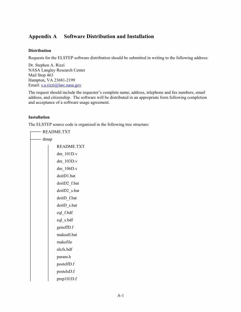
A-1

Appendix A Software Distribution and Installation Distribution Requests for the ELSTEP software distribution should be submitted in writing to the following address:

Dr. Stephen A. Rizzi NASA Langley Research Center Mail Stop 463 Hampton, VA 23681-2199 Email: s.a.rizzi@larc.nasa.gov

The request should include the requester�s complete name, address, telephone and fax numbers, email address, and citizenship. The software will be distributed in an appropriate form following completion and acceptance of a software usage agreement.

Installation The ELSTEP source code is organized in the following tree structure:

README.TXT

dmap

README.TXT

dm_101D.v

dm_103D.v

dm_106D.v

doitD1.bat

doitD2_f.bat

doitD2_s.bat

doitD_f.bat

doitD_s.bat

eql_f.bdf

eql_s.bdf

gensffD.f

makeall.bat

makefile

nlcfs.bdf

param.h

postelfD.f

postelsD.f

prep101D.f

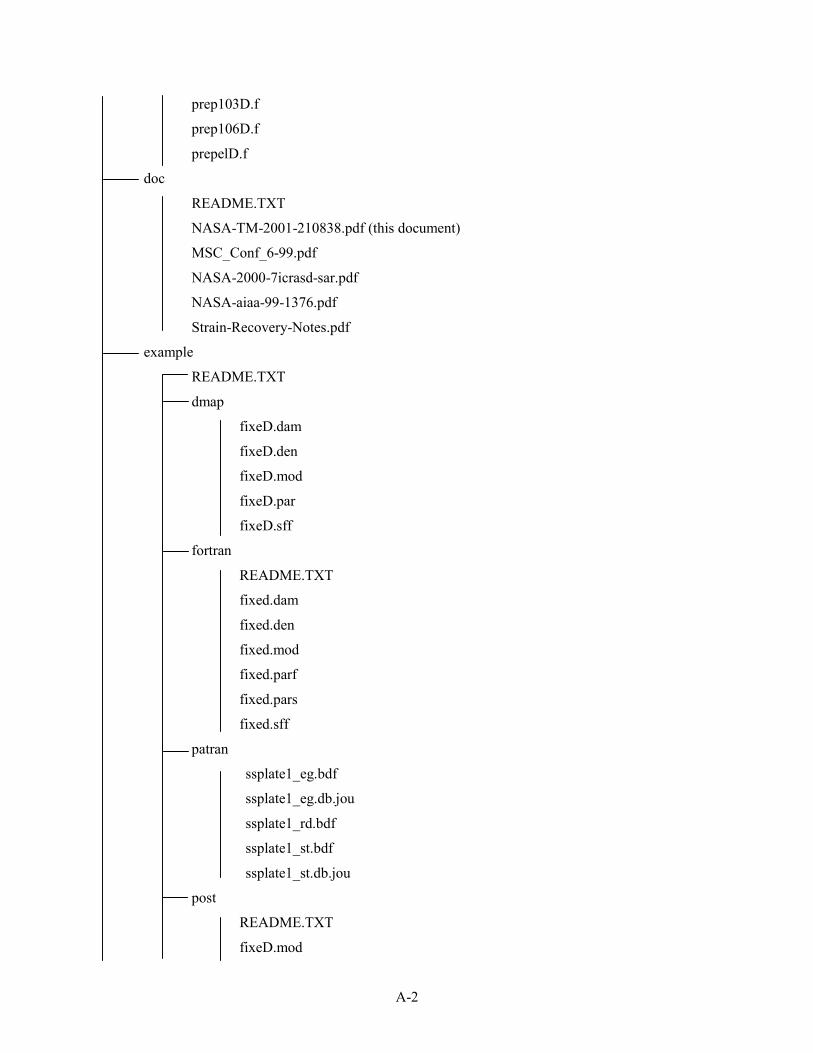
A-2

prep103D.f

prep106D.f

prepelD.f

doc

README.TXT

NASA-TM-2001-210838.pdf (this document)

MSC_Conf_6-99.pdf

NASA-2000-7icrasd-sar.pdf

NASA-aiaa-99-1376.pdf

Strain-Recovery-Notes.pdf

example

README.TXT

dmap

fixeD.dam

fixeD.den

fixeD.mod

fixeD.par

fixeD.sff

fortran

README.TXT

fixed.dam

fixed.den

fixed.mod

fixed.parf

fixed.pars

fixed.sff

patran

ssplate1_eg.bdf

ssplate1_eg.db.jou

ssplate1_rd.bdf

ssplate1_st.bdf

ssplate1_st.db.jou

post

README.TXT

fixeD.mod

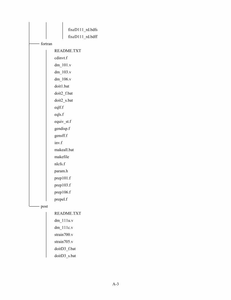
A-3

fixeD111_rd.bdfs

fixeD111_rd.bdff

fortran

README.TXT

cdinvt.f

dm_101.v

dm_103.v

dm_106.v

doit1.bat

doit2_f.bat

doit2_s.bat

eqlf.f

eqls.f

equiv_st.f

gendisp.f

gensff.f

inv.f

makeall.bat

makefile

nlcfs.f

param.h

prep101.f

prep103.f

prep106.f

prepel.f

post

README.TXT

dm_111u.v

dm_111c.v

strain700.v

strain705.v

doitD3_f.bat

doitD3_s.bat

A-4

The dmap directory off the main tree contains all the files required to run the DMAP implementation of the analysis. All FORTRAN utility programs contained in this directory are platform independent and should be compiled with a FORTRAN 90 compiler. The batch file makefile.bat will compile all FORTRAN programs using the UNIX �make� utility. Prior to compilation, the values for the maximum number of elements in the model (MAXEL), the maximum number of degrees of freedom in the model (NSX), the maximum number of eigenvectors specified in the normal modes analysis (NEIGX), and the maximum number of selected eigenvectors (NSELX) should be set sufficiently large in the file param.h. The DMAP implementation uses string-based Alters of NASTRAN version 70.0.0. It is therefore expected to be upward compatible with future versions of NASTRAN. Following compilation, the files should be copied to the directory in which the analysis is to be performed.

The fortran directory off the main tree contains all the files required to run the FORTRAN implementation of the analysis. All FORTRAN programs contained in this directory are platform independent and should be compiled with a FORTRAN 90 compiler. The batch file makefile.bat will compile all FORTRAN programs using the UNIX �make� utility. Prior to compilation, the values for the maximum number of elements in the model (MAXEL), the maximum number of degrees of freedom in the model (NSX), the maximum number of eigenvectors specified in the normal modes analysis (NEIGX), and the maximum number of selected eigenvectors (NSELX) should be set sufficiently large in the file param.h. Following compilation, the files should be copied to the directory in which the analysis is to be performed.

Note that since some of the files created in the DMAP and FORTRAN implementations have the same name, but differing content, the two implementations should be run in separate directories.

The post directory off the main tree contains all the files required to run the post processing analysis for either DMAP or FORTRAN implementations. These files should be copied to the directory in which the DMAP or FORTRAN analyses are performed. No compilation is required.

The doc directory off the main tree contains an Adobe Acrobat version of this document as well as Acrobat versions of references [10-12].

The example directory off the main tree contains the files required to run the simply support plate example problem used in this document. The dmap, fortran, and post sub-directories contain the input files required to run the DMAP, FORTRAN and post-processing analyses, respectively. The files in these directories should be copied to the appropriate analysis directory. The patran sub-directory contains PATRAN bulk data files and database journal files for the simply supported plate model. When running the example problem, two bulk data files (ssplate1_eg.bdf and ssplate1_st.bdf) should be copied to the analysis directory. The third bulk data file, ssplate1_rd.bdf, has already modified for post-processing as indicated in Section 2.3. The modified versions of this file are in the post sub-directory as fixeD111_rd.bdfs and fixeD111_rd.bdff for the strain-energy and force error minimization approaches. The only difference between the two files are the TABDMP1 card which indicates slightly different damping bounds to reflect the different shifts in fundamental frequency associated with the two different error minimization approaches. The appropriate one should be copied to the file fixeD111_rd.bdf in order to run the post-processing analysis. The PATRAN databases themselves may be re-created (if desired) using either the bulk data files or the database journal files.

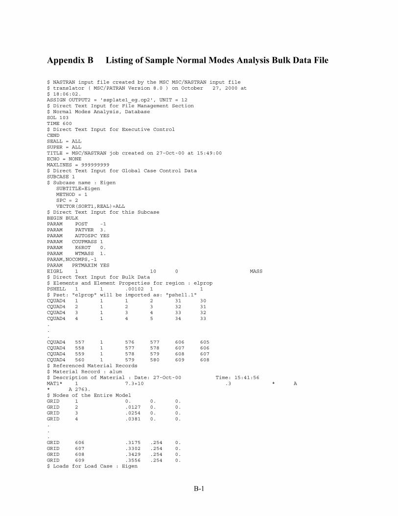
B-1

Appendix B Listing of Sample Normal Modes Analysis Bulk Data File $ NASTRAN input file created by the MSC MSC/NASTRAN input file$ translator ( MSC/PATRAN Version 8.0 ) on October 27, 2000 at$ 18:06:02.ASSIGN OUTPUT2 = 'ssplate1_eg.op2', UNIT = 12$ Direct Text Input for File Management Section$ Normal Modes Analysis, DatabaseSOL 103TIME 600$ Direct Text Input for Executive ControlCENDSEALL = ALLSUPER = ALLTITLE = MSC/NASTRAN job created on 27-Oct-00 at 15:49:00ECHO = NONEMAXLINES = 999999999$ Direct Text Input for Global Case Control DataSUBCASE 1$ Subcase name : Eigen

SUBTITLE=EigenMETHOD = 1SPC = 2VECTOR(SORT1,REAL)=ALL

$ Direct Text Input for this SubcaseBEGIN BULKPARAM POST -1PARAM PATVER 3.PARAM AUTOSPC YESPARAM COUPMASS 1PARAM K6ROT 0.PARAM WTMASS 1.PARAM,NOCOMPS,-1PARAM PRTMAXIM YESEIGRL 1 10 0 MASS$ Direct Text Input for Bulk Data$ Elements and Element Properties for region : elpropPSHELL 1 1 .00102 1 1$ Pset: "elprop" will be imported as: "pshell.1"CQUAD4 1 1 1 2 31 30CQUAD4 2 1 2 3 32 31CQUAD4 3 1 3 4 33 32CQUAD4 4 1 4 5 34 33...CQUAD4 557 1 576 577 606 605CQUAD4 558 1 577 578 607 606CQUAD4 559 1 578 579 608 607CQUAD4 560 1 579 580 609 608$ Referenced Material Records$ Material Record : alum$ Description of Material : Date: 27-Oct-00 Time: 15:41:56MAT1* 1 7.3+10 .3 * A* A 2763.$ Nodes of the Entire ModelGRID 1 0. 0. 0.GRID 2 .0127 0. 0.GRID 3 .0254 0. 0.GRID 4 .0381 0. 0....GRID 606 .3175 .254 0.GRID 607 .3302 .254 0.GRID 608 .3429 .254 0.GRID 609 .3556 .254 0.$ Loads for Load Case : Eigen

B-2

SPCADD 2 1 3 4 5$ Displacement Constraints of Load Set : x0simpleSPC1 1 134 1 30 59 88 117 146 + B+ B 175 204 233 262 291 320 349 378 + C+ C 407 436 465 494 523 552 581$ Displacement Constraints of Load Set : xlsimpleSPC1 3 134 29 58 87 116 145 174 + D+ D 203 232 261 290 319 348 377 406 + E+ E 435 464 493 522 551 580 609$ Displacement Constraints of Load Set : y0simpleSPC1 4 235 1 THRU 29$ Displacement Constraints of Load Set : ylsimpleSPC1 5 235 581 THRU 609$ Referenced Coordinate FramesENDDATA 15845f1b

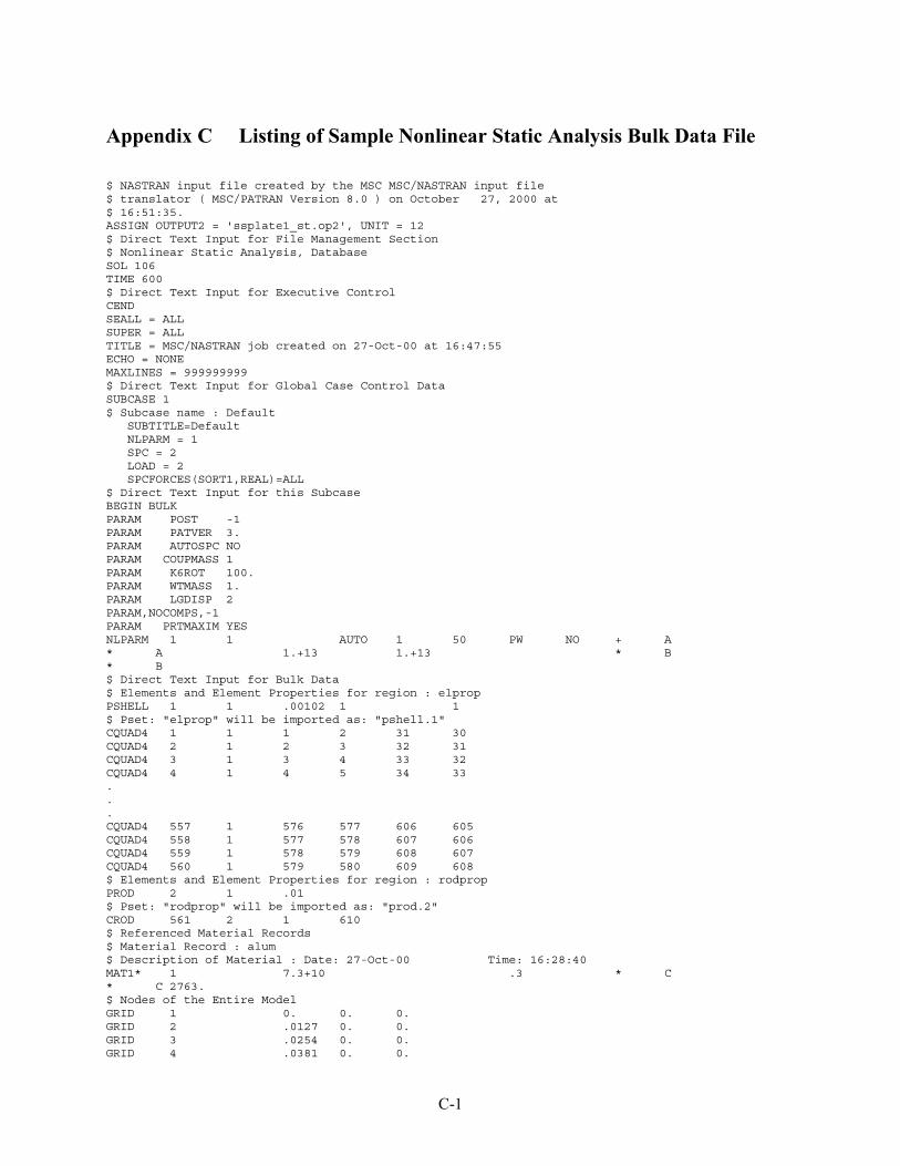
C-1

Appendix C Listing of Sample Nonlinear Static Analysis Bulk Data File $ NASTRAN input file created by the MSC MSC/NASTRAN input file$ translator ( MSC/PATRAN Version 8.0 ) on October 27, 2000 at$ 16:51:35.ASSIGN OUTPUT2 = 'ssplate1_st.op2', UNIT = 12$ Direct Text Input for File Management Section$ Nonlinear Static Analysis, DatabaseSOL 106TIME 600$ Direct Text Input for Executive ControlCENDSEALL = ALLSUPER = ALLTITLE = MSC/NASTRAN job created on 27-Oct-00 at 16:47:55ECHO = NONEMAXLINES = 999999999$ Direct Text Input for Global Case Control DataSUBCASE 1$ Subcase name : Default

SUBTITLE=DefaultNLPARM = 1SPC = 2LOAD = 2SPCFORCES(SORT1,REAL)=ALL

$ Direct Text Input for this SubcaseBEGIN BULKPARAM POST -1PARAM PATVER 3.PARAM AUTOSPC NOPARAM COUPMASS 1PARAM K6ROT 100.PARAM WTMASS 1.PARAM LGDISP 2PARAM,NOCOMPS,-1PARAM PRTMAXIM YESNLPARM 1 1 AUTO 1 50 PW NO + A* A 1.+13 1.+13 * B* B$ Direct Text Input for Bulk Data$ Elements and Element Properties for region : elpropPSHELL 1 1 .00102 1 1$ Pset: "elprop" will be imported as: "pshell.1"CQUAD4 1 1 1 2 31 30CQUAD4 2 1 2 3 32 31CQUAD4 3 1 3 4 33 32CQUAD4 4 1 4 5 34 33...CQUAD4 557 1 576 577 606 605CQUAD4 558 1 577 578 607 606CQUAD4 559 1 578 579 608 607CQUAD4 560 1 579 580 609 608$ Elements and Element Properties for region : rodpropPROD 2 1 .01$ Pset: "rodprop" will be imported as: "prod.2"CROD 561 2 1 610$ Referenced Material Records$ Material Record : alum$ Description of Material : Date: 27-Oct-00 Time: 16:28:40MAT1* 1 7.3+10 .3 * C* C 2763.$ Nodes of the Entire ModelGRID 1 0. 0. 0.GRID 2 .0127 0. 0.GRID 3 .0254 0. 0.GRID 4 .0381 0. 0.

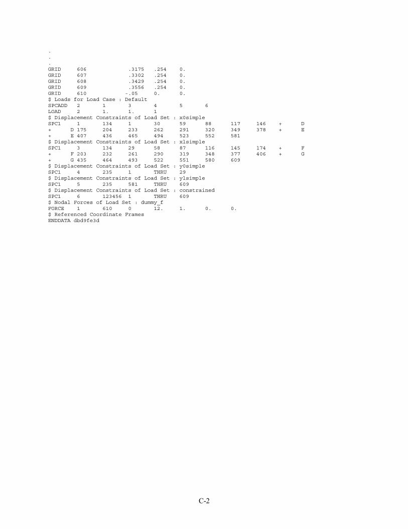
C-2

.

.

.GRID 606 .3175 .254 0.GRID 607 .3302 .254 0.GRID 608 .3429 .254 0.GRID 609 .3556 .254 0.GRID 610 -.05 0. 0.$ Loads for Load Case : DefaultSPCADD 2 1 3 4 5 6LOAD 2 1. 1. 1$ Displacement Constraints of Load Set : x0simpleSPC1 1 134 1 30 59 88 117 146 + D+ D 175 204 233 262 291 320 349 378 + E+ E 407 436 465 494 523 552 581$ Displacement Constraints of Load Set : xlsimpleSPC1 3 134 29 58 87 116 145 174 + F+ F 203 232 261 290 319 348 377 406 + G+ G 435 464 493 522 551 580 609$ Displacement Constraints of Load Set : y0simpleSPC1 4 235 1 THRU 29$ Displacement Constraints of Load Set : ylsimpleSPC1 5 235 581 THRU 609$ Displacement Constraints of Load Set : constrainedSPC1 6 123456 1 THRU 609$ Nodal Forces of Load Set : dummy_fFORCE 1 610 0 12. 1. 0. 0.$ Referenced Coordinate FramesENDDATA dbd9fe3d

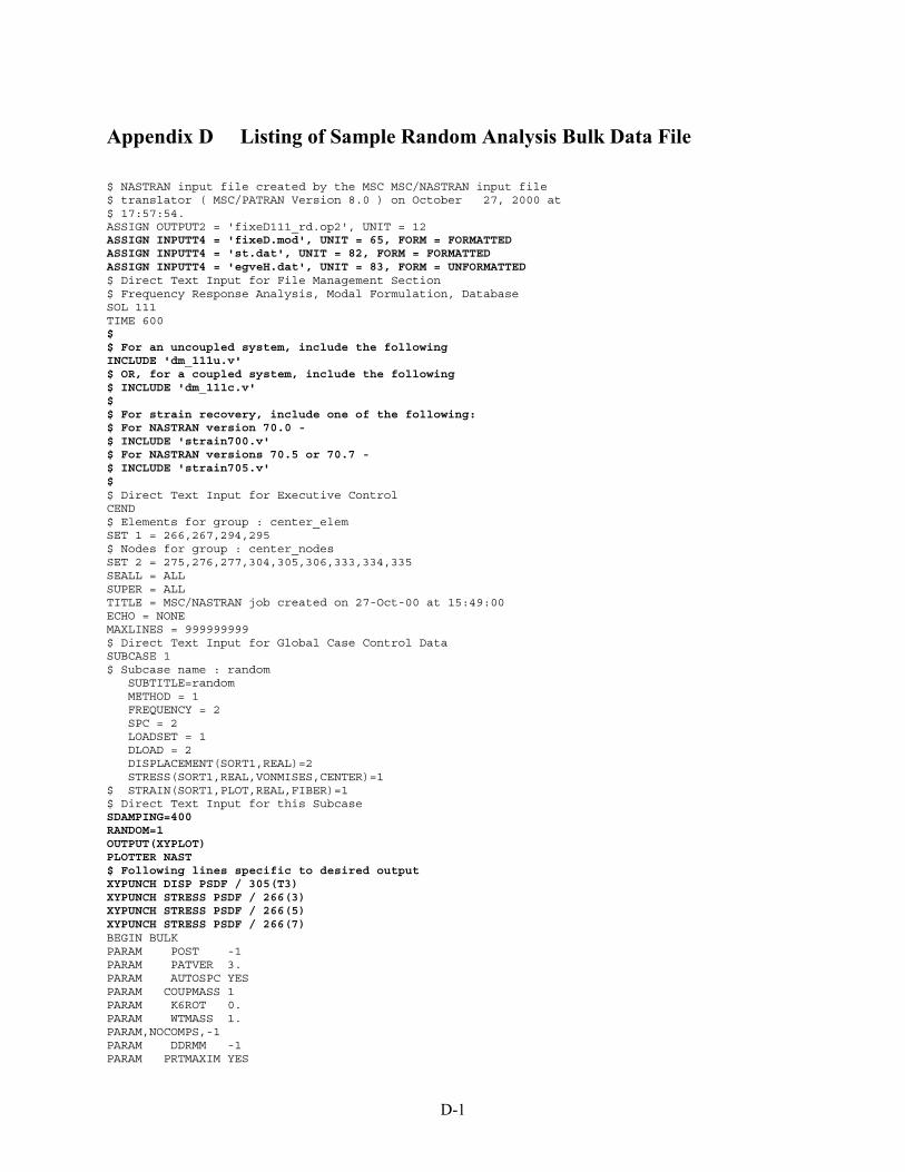
D-1

Appendix D Listing of Sample Random Analysis Bulk Data File $ NASTRAN input file created by the MSC MSC/NASTRAN input file$ translator ( MSC/PATRAN Version 8.0 ) on October 27, 2000 at$ 17:57:54.ASSIGN OUTPUT2 = 'fixeD111_rd.op2', UNIT = 12ASSIGN INPUTT4 = 'fixeD.mod', UNIT = 65, FORM = FORMATTEDASSIGN INPUTT4 = 'st.dat', UNIT = 82, FORM = FORMATTEDASSIGN INPUTT4 = 'egveH.dat', UNIT = 83, FORM = UNFORMATTED$ Direct Text Input for File Management Section$ Frequency Response Analysis, Modal Formulation, DatabaseSOL 111TIME 600$$ For an uncoupled system, include the followingINCLUDE 'dm_111u.v'$ OR, for a coupled system, include the following$ INCLUDE 'dm_111c.v'$$ For strain recovery, include one of the following:$ For NASTRAN version 70.0 -$ INCLUDE 'strain700.v'$ For NASTRAN versions 70.5 or 70.7 -$ INCLUDE 'strain705.v'$$ Direct Text Input for Executive ControlCEND$ Elements for group : center_elemSET 1 = 266,267,294,295$ Nodes for group : center_nodesSET 2 = 275,276,277,304,305,306,333,334,335SEALL = ALLSUPER = ALLTITLE = MSC/NASTRAN job created on 27-Oct-00 at 15:49:00ECHO = NONEMAXLINES = 999999999$ Direct Text Input for Global Case Control DataSUBCASE 1$ Subcase name : random

SUBTITLE=randomMETHOD = 1FREQUENCY = 2SPC = 2LOADSET = 1DLOAD = 2DISPLACEMENT(SORT1,REAL)=2STRESS(SORT1,REAL,VONMISES,CENTER)=1

$ STRAIN(SORT1,PLOT,REAL,FIBER)=1$ Direct Text Input for this SubcaseSDAMPING=400RANDOM=1OUTPUT(XYPLOT)PLOTTER NAST$ Following lines specific to desired outputXYPUNCH DISP PSDF / 305(T3)XYPUNCH STRESS PSDF / 266(3)XYPUNCH STRESS PSDF / 266(5)XYPUNCH STRESS PSDF / 266(7)BEGIN BULKPARAM POST -1PARAM PATVER 3.PARAM AUTOSPC YESPARAM COUPMASS 1PARAM K6ROT 0.PARAM WTMASS 1.PARAM,NOCOMPS,-1PARAM DDRMM -1PARAM PRTMAXIM YES

D-2

EIGRL 1 10 0FREQ1 2 0. .25 4096$ Direct Text Input for Bulk Data$ Elements and Element Properties for region : elpropPSHELL 1 1 .00102 1 1$ Pset: "elprop" will be imported as: "pshell.1"CQUAD4 1 1 1 2 31 30CQUAD4 2 1 2 3 32 31CQUAD4 3 1 3 4 33 32CQUAD4 4 1 4 5 34 33...CQUAD4 557 1 576 577 606 605CQUAD4 558 1 577 578 607 606CQUAD4 559 1 578 579 608 607CQUAD4 560 1 579 580 609 608$ Referenced Material Records$ Material Record : alum$ Description of Material : Date: 27-Oct-00 Time: 15:41:56MAT1* 1 7.3+10 .3 * A* A 2763.$ Nodes of the Entire ModelGRID 1 0. 0. 0.GRID 2 .0127 0. 0.GRID 3 .0254 0. 0.GRID 4 .0381 0. 0....GRID 606 .3175 .254 0.GRID 607 .3302 .254 0.GRID 608 .3429 .254 0.GRID 609 .3556 .254 0.$ Loads for Load Case : randomSPCADD 2 1 3 4 5RLOAD1 4 5 1LSEQ 1 5 3DLOAD 2 1. 1. 4$ Displacement Constraints of Load Set : x0simpleSPC1 1 134 1 30 59 88 117 146 + B+ B 175 204 233 262 291 320 349 378 + C+ C 407 436 465 494 523 552 581$ Displacement Constraints of Load Set : xlsimpleSPC1 3 134 29 58 87 116 145 174 + D+ D 203 232 261 290 319 348 377 406 + E+ E 435 464 493 522 551 580 609$ Displacement Constraints of Load Set : y0simpleSPC1 4 235 1 THRU 29$ Displacement Constraints of Load Set : ylsimpleSPC1 5 235 581 THRU 609$ Pressure Loads of Load Set : pressurePLOAD4 3 1 -1. THRU 560$ Referenced Dynamic Load Tables$ Constant Load TableTABLED1 1 + F+ F 0. 1. 1024. 1. ENDT$ -----------------------------------------------------$ RANDOM INPUT, flat spectrum (2048 Pa RMS, 0-1024 Hz = 160.2060 dB OASPL)$ -----------------------------------------------------RANDPS 1 1 1 1.0 0.0 101TABRND1 101 LINEAR LINEAR +TBR001+TBR001 0.0 4096.0 1024.0 4096.0 ENDT$ -----------------------------------------------------$ DAMPING TABLE, constant over frequency$ -----------------------------------------------------TABDMP1 400 CRIT +DP1+DP1 0.0 0.02 446.0 0.02 446.00 0.0054 SKIP +DP2+DP2 1024.0 0.0054 ENDT$ Referenced Coordinate FramesENDDATA b72b05e7

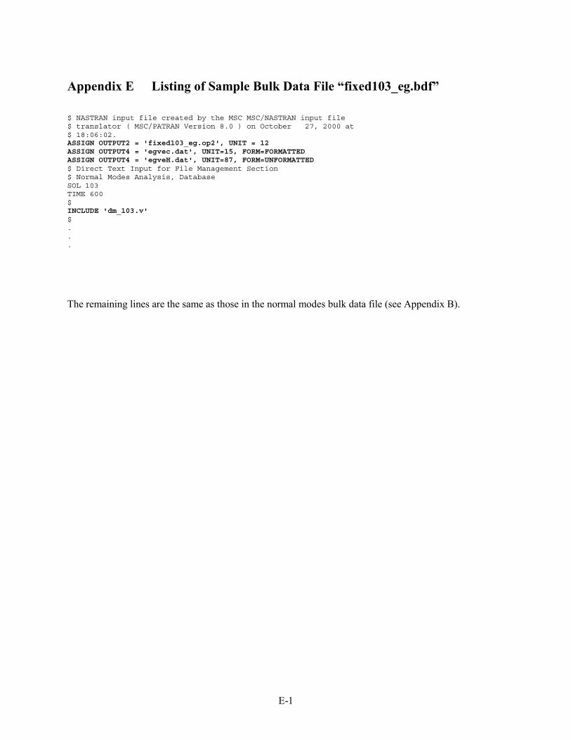
E-1

Appendix E Listing of Sample Bulk Data File �fixed103_eg.bdf� $ NASTRAN input file created by the MSC MSC/NASTRAN input file$ translator ( MSC/PATRAN Version 8.0 ) on October 27, 2000 at$ 18:06:02.ASSIGN OUTPUT2 = 'fixed103_eg.op2', UNIT = 12ASSIGN OUTPUT4 = 'egvec.dat', UNIT=15, FORM=FORMATTEDASSIGN OUTPUT4 = 'egveH.dat', UNIT=87, FORM=UNFORMATTED$ Direct Text Input for File Management Section$ Normal Modes Analysis, DatabaseSOL 103TIME 600$INCLUDE 'dm_103.v'$...

The remaining lines are the same as those in the normal modes bulk data file (see Appendix B).

F-1

Appendix F Listing of Sample Bulk Data File �fixed106_st.bdf� $ NASTRAN input file created by the MSC MSC/NASTRAN input file$ translator ( MSC/PATRAN Version 8.0 ) on October 27, 2000 at$ 16:51:35.ASSIGN OUTPUT2 = 'fixed106_st.op2', UNIT = 12ASSIGN OUTPUT4 = 'f_N.frc', UNIT = 15 , FORM=FORMATTEDASSIGN INPUTT4 = 'displ.inn', UNIT = 17 , FORM=FORMATTED$ Direct Text Input for File Management Section$ Nonlinear Static Analysis, DatabaseSOL 106TIME 600$INCLUDE 'dm_106.v'$$ Direct Text Input for Executive ControlCENDSEALL = ALLSUPER = ALLTITLE = MSC/NASTRAN job created on 27-Oct-00 at 16:47:55ECHO = NONEMAXLINES = 999999999$ Direct Text Input for Global Case Control DataSUBCASE 1$ Subcase name : Default

SUBTITLE=DefaultNLPARM = 1SPC = 2LOAD = 2SPCFORCES(SORT1,REAL)=ALL

SUBCASE 2$ Subcase name : Default

SUBTITLE=DefaultNLPARM = 1SPC = 2LOAD = 2SPCFORCES(SORT1,REAL)=ALL

SUBCASE 3$ Subcase name : Default

SUBTITLE=DefaultNLPARM = 1SPC = 2LOAD = 2SPCFORCES(SORT1,REAL)=ALL

SUBCASE 4$ Subcase name : Default

SUBTITLE=DefaultNLPARM = 1SPC = 2LOAD = 2SPCFORCES(SORT1,REAL)=ALL

SUBCASE 5$ Subcase name : Default

SUBTITLE=DefaultNLPARM = 1SPC = 2LOAD = 2SPCFORCES(SORT1,REAL)=ALL

SUBCASE 6$ Subcase name : Default

SUBTITLE=DefaultNLPARM = 1SPC = 2LOAD = 2SPCFORCES(SORT1,REAL)=ALL

SUBCASE 7$ Subcase name : Default

SUBTITLE=Default

F-2

NLPARM = 1SPC = 2LOAD = 2SPCFORCES(SORT1,REAL)=ALL

$ Direct Text Input for this SubcaseBEGIN BULK...

The remaining lines are the same as those in the static analysis bulk data file (see Appendix C).

G-1

Appendix G Listing of Sample Bulk Data File �fixed101_st.bdf� $ NASTRAN input file created by the MSC MSC/NASTRAN input file$ translator ( MSC/PATRAN Version 8.0 ) on October 27, 2000 at$ 16:51:35.ASSIGN OUTPUT2 = 'fixed101_st.op2', UNIT = 12ASSIGN OUTPUT4 = 'f1_L.frc', UNIT = 15 , FORM=FORMATTEDASSIGN INPUTT4 = 'dispL.inn', UNIT = 17 , FORM=FORMATTED$ Direct Text Input for File Management Section$ Nonlinear Static Analysis, DatabaseSOL 101TIME 600$INCLUDE 'dm_101.v'$$ Direct Text Input for Executive ControlCENDSEALL = ALLSUPER = ALLTITLE = MSC/NASTRAN job created on 27-Oct-00 at 16:47:55ECHO = NONEMAXLINES = 999999999$ Direct Text Input for Global Case Control DataSUBCASE 1$ Subcase name : Default

SUBTITLE=DefaultNLPARM = 1SPC = 2LOAD = 2SPCFORCES(SORT1,REAL)=ALL

SUBCASE 2$ Subcase name : Default

SUBTITLE=DefaultNLPARM = 1SPC = 2LOAD = 2SPCFORCES(SORT1,REAL)=ALL

$ Direct Text Input for this SubcaseBEGIN BULK...

The remaining lines are the same as those in the static analysis bulk data file (see Appendix C).

H-1

Appendix H Listing of Sample Bulk Data File �fixeD103_eg.bdf� $ NASTRAN input file created by the MSC MSC/NASTRAN input file$ translator ( MSC/PATRAN Version 8.0 ) on October 27, 2000 at$ 18:06:02.ASSIGN OUTPUT2 = 'fixeD103_eg.op2', UNIT = 12ASSIGN OUTPUT4 = 'egvec.dat',UNIT = 15,FORM=UNFORMATTEDASSIGN INPUTT4 = 'fixeD.mod',UNIT = 65,FORM=FORMATTEDASSIGN OUTPUT4 = 'displ.pr2',UNIT = 79,FORM=FORMATTEDASSIGN OUTPUT4 = 'displ.pr3',UNIT = 80,FORM=FORMATTEDASSIGN OUTPUT4 = 'displ.pr4',UNIT = 78,FORM=FORMATTEDASSIGN OUTPUT4 = 'displ.inn',UNIT = 81,FORM=UNFORMATTEDASSIGN OUTPUT4 = 'dispL.inn',UNIT = 82,FORM=UNFORMATTEDASSIGN OUTPUT4 = 'egveC.dat',UNIT = 77,FORM=UNFORMATTEDASSIGN OUTPUT4 = 'egveH.dat',UNIT = 87,FORM=UNFORMATTEDASSIGN OUTPUT4 = 'egveCa.dat',UNIT = 83,FORM=FORMATTED$ Direct Text Input for File Management Section$ Normal Modes Analysis, DatabaseSOL 103TIME 600$INCLUDE 'dm_103D.v'$...

The remaining lines are the same as those in the normal modes bulk data file (see Appendix B).

I-1

Appendix I Listing of Sample Bulk Data File �fixeD106_st.bdf� $ NASTRAN input file created by the MSC MSC/NASTRAN input file$ translator ( MSC/PATRAN Version 8.0 ) on October 27, 2000 at$ 16:51:35.ASSIGN OUTPUT2 = 'fixeD106_st.op2', UNIT = 12ASSIGN OUTPUT4 = 'f_N.frc',UNIT = 15 ,FORM=UNFORMATTEDASSIGN INPUTT4 = 'displ.inn',UNIT = 17 ,FORM=UNFORMATTED$ Direct Text Input for File Management Section$ Nonlinear Static Analysis, DatabaseSOL 106TIME 600$INCLUDE 'dm_106D.v'$$ Direct Text Input for Executive ControlCENDSEALL = ALLSUPER = ALLTITLE = MSC/NASTRAN job created on 27-Oct-00 at 16:47:55ECHO = NONEMAXLINES = 999999999$ Direct Text Input for Global Case Control DataSUBCASE 1$ Subcase name : Default

SUBTITLE=DefaultNLPARM = 1SPC = 2LOAD = 2SPCFORCES(SORT1,REAL)=ALL

SUBCASE 2$ Subcase name : Default

SUBTITLE=DefaultNLPARM = 1SPC = 2LOAD = 2SPCFORCES(SORT1,REAL)=ALL

SUBCASE 3$ Subcase name : Default

SUBTITLE=DefaultNLPARM = 1SPC = 2LOAD = 2SPCFORCES(SORT1,REAL)=ALL

SUBCASE 4$ Subcase name : Default

SUBTITLE=DefaultNLPARM = 1SPC = 2LOAD = 2SPCFORCES(SORT1,REAL)=ALL

SUBCASE 5$ Subcase name : Default

SUBTITLE=DefaultNLPARM = 1SPC = 2LOAD = 2SPCFORCES(SORT1,REAL)=ALL

SUBCASE 6$ Subcase name : Default

SUBTITLE=DefaultNLPARM = 1SPC = 2LOAD = 2SPCFORCES(SORT1,REAL)=ALL

SUBCASE 7$ Subcase name : Default

SUBTITLE=Default

I-2

NLPARM = 1SPC = 2LOAD = 2SPCFORCES(SORT1,REAL)=ALL

$ Direct Text Input for this SubcaseBEGIN BULK...

The remaining lines are the same as those in the static analysis bulk data file (see Appendix C).

J-1

Appendix J Listing of Sample Bulk Data File �fixeD101_st.bdf� $ NASTRAN input file created by the MSC MSC/NASTRAN input file$ translator ( MSC/PATRAN Version 8.0 ) on October 27, 2000 at$ 16:51:35.ASSIGN OUTPUT2 = 'fixeD101_st.op2', UNIT = 12ASSIGN OUTPUT4 = 'f1_L.frc',UNIT = 15,FORM=UNFORMATTEDASSIGN INPUTT4 = 'dispL.inn',UNIT = 17,FORM=UNFORMATTED$ Direct Text Input for File Management Section$ Nonlinear Static Analysis, DatabaseSOL 101TIME 600$INCLUDE 'dm_101D.v'$$ Direct Text Input for Executive ControlCENDSEALL = ALLSUPER = ALLTITLE = MSC/NASTRAN job created on 27-Oct-00 at 16:47:55ECHO = NONEMAXLINES = 999999999$ Direct Text Input for Global Case Control DataSUBCASE 1$ Subcase name : Default

SUBTITLE=DefaultNLPARM = 1SPC = 2LOAD = 2SPCFORCES(SORT1,REAL)=ALL

SUBCASE 2$ Subcase name : Default

SUBTITLE=DefaultNLPARM = 1SPC = 2LOAD = 2SPCFORCES(SORT1,REAL)=ALL

$ Direct Text Input for this SubcaseBEGIN BULK...

The remaining lines are the same as those in the static analysis bulk data file (see Appendix C).

REPORT DOCUMENTATION PAGE Form Approved OMB No. 0704-0188

Public reporting burden for this collection of information is estimated to average 1 hour per response, including the time for reviewing instructions, searching existing data sources, gathering and maintaining the data needed, and completing and reviewing the collection of information. Send comments regarding this burden estimate or any other aspect of this collection of information, including suggestions for reducing this burden, to Washington Headquarters Services, Directorate for Information Operations and Reports, 1215 Jefferson Davis Highway, Suite 1204, Arlington, VA 22202-4302, and to the Office of Management and Budget, Paperwork Reduction Project (0704-0188), Washington, DC 20503. 1. AGENCY USE ONLY (Leave blank)

2. REPORT DATE

March 2001 3. REPORT TYPE AND DATES COVERED

Technical Memorandum 4. TITLE AND SUBTITLE

Improved Equivalent Linearization Implementations Using Nonlinear Stiffness Evaluation

5. FUNDING NUMBERS 522-63-11-03

6. AUTHOR(S) Stephen A. Rizzi Alexander A. Muravyov

7. PERFORMING ORGANIZATION NAME(S) AND ADDRESS(ES)

National Aeronautics and Space Administration Langley Research Center Hampton, VA 23681-2199

8. PERFORMING ORGANIZATION REPORT NUMBER

L-18068

9. SPONSORING/MONITORING AGENCY NAME(S) AND ADDRESS(ES)

National Aeronautics and Space Administration Langley Research Center Hampton, VA 23681-2199

10. SPONSORING/MONITORING AGENCY REPORT NUMBER

NASA/TM-2001-210838

11. SUPPLEMENTARY NOTES Alexander Muravyov was an National Research Council post-doctoral research associate at the NASA Langley Research Center from June 1998 to September 1999.

12a. DISTRIBUTION/AVAILABILITY STATEMENT Unclassified-Unlimited Subject Category 39 Distribution: Standard Availability: NASA CASI (301) 621-0390

12b. DISTRIBUTION CODE

13. ABSTRACT (Maximum 200 words) This report documents two new implementations of equivalent linearization for solving geometrically nonlinear random vibration problems of complicated structures. The implementations are given the acronym ELSTEP, for �Equivalent Linearization using a STiffness Evaluation Procedure.� Both implementations of ELSTEP are fundamentally the same in that they use a novel nonlinear stiffness evaluation procedure to numerically compute otherwise inaccessible nonlinear stiffness terms from commercial finite element programs. The commercial finite element program MSC/NASTRAN (NASTRAN) was chosen as the core of ELSTEP. The FORTRAN implementation calculates the nonlinear stiffness terms and performs the equivalent linearization analysis outside of NASTRAN. The Direct Matrix Abstraction Program (DMAP) implementation performs these operations within NASTRAN. Both provide nearly identical results. Within each implementation, two error minimization approaches for the equivalent linearization procedure are available � force and strain energy error minimization. Sample results for a simply supported rectangular plate are included to illustrate the analysis procedure.

15. NUMBER OF PAGES 66

14. SUBJECT TERMS Geometrically nonlinear random vibration, equivalent linearization, statistical linearization, force error minimization, strain-energy error minimization, sonic fatigue

16. PRICE CODE A04

17. SECURITY CLASSIFICATION OF REPORT Unclassified

18. SECURITY CLASSIFICATION OF THIS PAGE Unclassified

19. SECURITY CLASSIFICATION OF ABSTRACT Unclassified

20. LIMITATION OF ABSTRACT UL

NSN 7540-01-280-5500 Standard Form 298 (Rev. 2-89) Prescribed by ANSI Std. Z-39-18 298-102