Imprints of relic gravitational waves in cosmic microwave

Imprints of relic gravitational waves in cosmic microwave background radiation

D. BaskaranSchool of Physics and Astronomy, Cardiff University, Cardiff CF24 3YB, United Kingdom

L. P. GrishchukSchool of Physics and Astronomy, Cardiff University, Cardiff CF24 3YB, United Kingdomand Sternberg Astronomical Institute, Moscow State University, Moscow 119899, Russia

A. G. PolnarevAstronomy Unit, School of Mathematical Sciences Queen Mary, University of London, Mile End Road,

London E1 4NS, United Kingdom(Received 18 May 2006; published 27 October 2006)

A strong variable gravitational field of the very early Universe inevitably generates relic gravitationalwaves by amplifying their zero-point quantum oscillations. We begin our discussion by contrasting theconcepts of relic gravitational waves and inflationary ‘‘tensor modes’’. We explain and summarize theproperties of relic gravitational waves that are needed to derive their effects on cosmic microwavebackground (CMB) temperature and polarization anisotropies. The radiation field is characterized by fourinvariants I, V, E, B. We reduce the radiative transfer equations to a single integral equation of Voltairretype and solve it analytically and numerically. We formulate the correlation functions CXX

0

‘ for X, X0 T,E, B and derive their amplitudes, shapes and oscillatory features. Although all of our main conclusions aresupported by exact numerical calculations, we obtain them, in effect, analytically by developing and usingaccurate approximations. We show that the TE correlation at lower ‘’s must be negative (i.e. ananticorrelation), if it is caused by gravitational waves, and positive if it is caused by density perturbations.This difference in TE correlation may be a signature more valuable observationally than the lack orpresence of the BB correlation, since the TE signal is about 100 times stronger than the expected BBsignal. We discuss the detection by WMAP of the TE anticorrelation at ‘ 30 and show that such ananticorrelation is possible only in the presence of a significant amount of relic gravitational waves (withinthe framework of all other common assumptions). We propose models containing considerable amounts ofrelic gravitational waves that are consistent with the measured TT, TE and EE correlations.

DOI: 10.1103/PhysRevD.74.083008 PACS numbers: 98.70.Vc, 04.30.w, 98.80.Cq

I. INTRODUCTION

The detection of primordial gravitational waves isrightly considered a highest priority task for the upcomingobservational missions [1]. Relic gravitational waves areinevitably generated by strong variable gravitational fieldof the very early Universe. The generating mechanism isthe superadiabatic (parametric) amplification of the waves’zero-point quantum oscillations [2]. In contrast to otherknown massless particles, the coupling of gravitationalwaves to the ‘‘external’’ gravitational field is such thatthey could be amplified or generated in a homogeneousisotropic FLRW (Friedmann-Lemaitre-Robertson-Walker)universe. This conclusion, at the time of its formulation,was on a collision course with the dominating theoreticaldoctrine. At that time, it was believed that the gravitationalwaves could not be generated in a FLRW universe, and thepossibility of their generation required the early Universeto be strongly anisotropic (see, for example, [3]).

The generating mechanism itself relies only on thevalidity of general relativity and quantum mechanics. Butthe amount and spectral content of relic gravitationalwaves depend on a specific evolution of the cosmologicalscale factor (classical ‘‘pumping’’ gravitational field) a.

The theory was applied to a variety of a, includingthose that are now called inflationary models (for a sampleof possible spectra of relic gravitational waves, see Fig. 4in Ref. [4]). If a unique a were known in advance fromsome fundamental ‘‘theory of everything’’, we would havederived the properties of the today’s signal with no ambi-guity. In the absence of such a theory, we have to use theavailable partial information in order to reduce the numberof options. This allows us to evaluate the level of theexpected signals in various frequency intervals. The prizeis very high—the actual detection of a particular back-ground of relic gravitational waves will provide us with theunique clue to the ‘‘birth’’ of the Universe and its veryearly dynamical behavior.

A crucial assumption that we make in this and previousstudies is that the observed large-scale cosmic microwavebackground (CMB) anisotropies are caused by cosmologi-cal perturbations of quantum-mechanical origin. If this istrue, then general relativity and quantum mechanics tell usthat relic gravitational waves should be a significant, if nota dominant, contributor to the observed large-scale anisot-ropies. From the existing data on the amplitude and spec-trum of the CMB fluctuations we infer the amplitude andspectral slope of the very long relic gravitational waves.

PHYSICAL REVIEW D 74, 083008 (2006)

1550-7998=2006=74(8)=083008(32) 083008-1 © 2006 The American Physical Society

http://dx.doi.org/10.1103/PhysRevD.74.083008

We then derive detailed predictions for indirect and directobservations of relic gravitational waves in various fre-quency bands.

At this point, it is important to clarify the differencebetween the concepts of relic gravitational waves and whatis now called inflationary gravitational waves. The state-ments about inflationary gravitational waves (‘‘tensormodes’’) are based on the inflation theory. This theoryassumes that the evolution of the very early Universe wasdriven by a scalar field, coupled to gravity in a specialmanner. The theory does not deny the correctness of thepreviously performed calculations for relic gravitationalwaves. However, the inflationary theory proposes its ownway of calculating the generation of density perturbations(‘‘scalar modes’’). The inflationary theory appeals exactlyto the same mechanism of superadiabatic (parametric)amplification of quantum vacuum fluctuations, that is re-sponsible for the generation of relic gravitational waves,but enforces very peculiar initial conditions in the scalarmodes calculations.

According to the inflationary initial conditions, the am-plitudes of the ‘gauge-invariant’ metric perturbations associated with the scalar modes (or, in other words, theamplitudes of the curvature perturbations called or R)can be arbitrarily large from the very beginning of theirevolution. Moreover, the theory demands that these ampli-tudes must be infinitely large in the limit of the deSitterexpansion law a / jj1 which is responsible for thegeneration of a flat (Harrison-Zeldovich-Peebles, ‘scale-invariant’) primordial spectrum, with the spectral indexn 1. At the same time, the amplitudes of the generatedgravitational waves are finite and small for all spectralindices, including n 1. Since both, gravitational wavesand density perturbations, produce CMB anisotropies andwe see them small today, the inflationary theory substitutes(for ‘‘consistency’’) its prediction of infinitely large ampli-tudes of density perturbations, in the limit n 1, by theclaim that it is the amount of primordial gravitationalwaves, expressed in terms of the ‘tensor/scalar ratio r0,that should be zero, r 0. For a detailed critical analysisof the inflationary conclusions, see [5]; for argumentsaimed at defending those conclusions, see [6].

The science motivations and CMB data analysis pipe-lines, designed to evaluate the gravitational-wave contri-bution, are usually based on inflationary formulas [7–10].In particular, according to the inflation theory, the primor-dial power spectrum of density perturbations has the form(it follows, for example, from Eqs. (2.12a) and (2.12b) inRef. [10] or from Eqs. (18) and (19) (or A12 and A13) inRef. [7]):

PSk 1

43M2Pl

1

rH2jkaH:

Despite the fact that this spectrum diverges at r 0 (ns 1, nt 0), the CMB data analysts persistently claim that

the inflation theory is in spectacular agreement with ob-servations and the CMB data are perfectly well consistentwith r 0 (the published confidence level contours alwaysinclude r 0 and are typically centered at that point).

Our analysis in this paper, based on general relativityand quantum mechanics, is aimed at showing that there isevidence of signatures of relic gravitational waves in thealready available CMB data. We also make predictions forsome future experiments and observations.

The plan of the paper is as follows. In Sec. II wesummarize the properties of a random background of relicgravitational waves that are needed for CMB calculations.The emphasis is on the gravitational wave (g.w.) modefunctions, power spectra, and statistical relations. InSec. III we discuss the general equations of radiative trans-fer and explain the existence of four invariants I, V, E, Bthat fully characterize the radiation field. We formulate thelinearized equations in the presence of a single Fouriermode of gravitational waves. We prove that there exists achoice of variables that reduces the problem of temperatureand polarization anisotropies to only two functions of time and .

Section IV is devoted to further analysis of the radiativetransfer equations. The main result of this section is thereduction of coupled integro-differential equations to asingle integral equation of Voltairre type. Essentially, theentire problem of the CMB polarization is reduced to asingle integral equation. This allows us to use simpleanalytical approximations and give transparent physicalinterpretation. In Sec. V we generalize the analysis to asuperposition of random Fourier modes with arbitrarywave vectors. We derive (and partially rederive the previ-ously known) expressions for multipole coefficients aX‘m ofthe radiation field. We show that the statistical properties ofthe multipole coefficients are fully determined by thestatistical properties of the underlying gravitational pertur-bations. This section contains the expressions for generalcorrelation and cross-correlation functions CXX

0

‘ for invar-iants of the radiation field.

We work out astrophysical applications in Secs. VI andVII where we discuss the effects of recombination andreionization era, respectively. Although all our main con-clusions are supported by exact numerical calculations, weshow the origin of these conclusions and essentially derivethem by developing and using semianalytical approxima-tions. The expected amplitudes, shapes, oscillatory fea-tures, etc. of all correlation functions as functions of ‘are under analytical control. The central point of thisanalysis is the TE correlation function. We show that, atlower multipoles ‘, the TE correlation function must benegative (anticorrelation), if it is induced by gravitationalwaves, and positive, if it is induced by density perturba-tions. We argue that this difference in sign of TE correla-tions can be a signature more valuable observationally thanthe presence or absence of the BB correlations. This is

D. BASKARAN, L. P. GRISHCHUK, AND A. G. POLNAREV PHYSICAL REVIEW D 74, 083008 (2006)

083008-2

because the TE signal is about 2 orders of magnitude largerthan the expected BB signal and is much easier to measure.We summarize the competing effects of density perturba-tions in Appendix D.

Theoretical findings are compared with observations inSec. VIII. In the context of relic gravitational waves it isespecially important that the WMAP team [9] stresses(even if for a different reason) the actual detection of theTE anticorrelation near ‘ 30. We show that this ispossible only in the presence of a significant amount ofrelic gravitational waves (within the framework of all othercommon assumptions). We analyze the CMB data andsuggest models with significant amounts of gravitationalwaves that are consistent with the measured TT, TE andEE correlation functions. Our final conclusion is that thereis evidence of the presence of relic gravitational waves inthe already available CMB data, and further study of theTE correlation at lower ‘’s has the potential of a firmpositive answer.

II. GENERAL PROPERTIES OF RELICGRAVITATIONAL WAVES

Here we summarize some properties of cosmologicalperturbations of quantum-mechanical origin. We will needformulas from this summary for our further calculations.

A. Basic definitions

As usual (for more details, see, for example, [11]), wewrite the perturbed gravitational field of a flat FLRWuniverse in the form

ds2 c2dt2 a2tij hijdxidxj

a2d2 ij hijdxidxj: (1)

We denote the present moment of time by R anddefine it by the observed quantities, for example, by to-day’s value of the Hubble parameter H0 HR. Inaddition, we take the present-day value of the scale factorto be aR 2lH, where lH c=H0.

The functions hij;x are expanded over spatialFourier harmonics einx, where n is a dimensionlesstime independent wave vector. The wave number n is n ijninj1=2. The wavelength , measured in units of labo-ratory standards, is related to n by 2a=n. The waveswhose wavelengths today are equal to today’s Hubbleradius carry the wave number nH 4. Shorter waveshave larger n’s and longer waves have smaller n’s.

The often used dimensional wave number k, defined byk 2=R in terms of today’s wavelength R, isrelated to n by a simple formula

k n

2lH n1:66 104h Mpc1:

The expansion of the field hij;x over Fourier com-ponents n requires a specification of polarization tensors

psijn s 1; 2. They have different forms depending on

whether the functions hij;x represent gravitationalwaves, rotational perturbations, or density perturbations.

In the case of gravitational waves, two independentlinear polarization states can be described by two realpolarization tensors

p1ijn lilj mimj; p

2ijn limj milj; (2)

where spatial vectors l;m;n=n are unit and mutuallyorthogonal vectors. The polarization tensors (2) satisfythe conditions

psijij 0; p

sijni 0; p

s0

ijps ij 2s0s: (3)

The eigenvectors of p1ij are li and mi, whereas the eigen-

vectors of p2ij are li mi and li mi. In both cases, the

first eigenvector has the eigenvalue 1, whereas the sec-ond eigenvector has the eigenvalue 1.

In terms of spherical coordinates , , we choose forl;m;n=n the right-handed triplet:

l cos cos; cos sin; sin;

m sin; cos; 0;

n=n sin cos; sin sin; cos:

(4)

The vector l points along a meridian in the direction ofincreasing , while the vector m points along a parallel inthe direction of increasing . With this specification, po-larization tensors (2) will be called the ‘’ and ‘’ polar-izations. The eigenvectors of ‘’ polarization correspondto north-south and east-west directions, whereas the ‘’polarization describes the directions rotated by 45.

With a fixed n, the choice of vectors l, m given byEq. (4) is not unique. The vectors can be subject to con-tinuous and discrete transformations. The continuoustransformation is performed by a rotation of the pair l, min the plane orthogonal to n:

l 0 l cos m sin ; m0 l sin m cos ;

(5)

where is an arbitrary angle. The discrete transformationis described by the flips of the l, m vectors:

l 0 l; m0 m or l0 l; m0 m:

(6)

When (5) is applied, polarization tensors (2) transform as

p1 0

ijn l0il0j m

0im0j p

1ijn cos2 p

2ijn sin2 ;

p2 0

ijn l0im0j m

0il0j p

1ijn sin2 p

2ijn cos2 ;

(7)

and when (6) is applied they transform as

IMPRINTS OF RELIC GRAVITATIONAL WAVES IN . . . PHYSICAL REVIEW D 74, 083008 (2006)

083008-3

p1 0ijn p

1ijn; p

2 0

ijn p2ijn: (8)

Later in this section and in Appendix A, we are discus-sing the conditions under which the averaged observationalproperties of a random field hijn; are symmetric withrespect to rotations around the axis n=n and with respect tomirror reflections of the axes. Formally, this is expressed asthe requirement of symmetry of the g.w. field correlationfunctions with respect to transformations (5) and (6).

In this paper we will also be dealing with density per-turbations. In this case, the polarization tensors are

p1ij

2

3

sij; p

2ij

3p ninj

n2 13p ij: (9)

These polarization tensors satisfy the last of the conditions(3).

In the rigorous quantum-mechanical version of the the-ory, the functions hij are quantum-mechanical operators.We write them in the form:

hij;x C

23=2

Z 11

d3n12np

Xs1;2

psijnh

s

neinxc

sn

psij nh

s

n

einxc

syn; (10)

where the annihilation and creation operators, cs

n and csy

n,satisfy the relationships

cs0

n; csy

n0 s0s3n n0; cs

nj0i 0: (11)

The initial vacuum state j0i of perturbations is defined atsome moment of time 0 in the remote past, long beforethe onset of the process of superadiabatic amplification.This quantum state is maintained (in the Heisenberg pic-ture) until now. For gravitational waves, the normalizationconstant is C

16p

lPl.The relationships (11) determine the expectation values

and correlation functions of cosmological perturbationsthemselves, and also of the CMB’s temperature and polar-ization anisotropies caused by these cosmological pertur-bations. In particular, the variance of metric perturbationsis given by

h0jhij;xhij;xj0i C2

22

Z 10n2

Xs1;2

jhs

nj2 dnn:

(12)

The quantity

h2n; C2

22 n2Xs1;2

jhs

nj2

1

2

Xs1;2

jhsn; j2; (13)

is called the metric power spectrum. Note that we haveintroduced

hsn;

C

nhs

n: (14)

The quantity (13) gives the mean-square value of thegravitational-field perturbations in a logarithmic intervalof n. The spectrum of the root-mean-square (rms) ampli-tude hn; is determined by the square root of Eq. (13).

Having evolved the classical mode functions hs

n up tosome arbitrary instant of time (for instance, today R) one can find the power spectrum hn; at that instantof time. For the today’s spectrum in terms of frequency measured in Hz, nH0=4, we use the notation hrms.

In our further applications we will also need the powerspectrum of the first time-derivative of metric perturba-tions:

0

@hij;x@@hij;x

@

0

1

2

Z 10

Xs1;2

dhsn; d

2dnn: (15)

To simplify calculations, in the rest of the paper we willbe using a ‘‘classical’’ version of the theory, whereby the

quantum-mechanical operators cs

n and csy

n are treated as

classical random complex numbers cs

n and cs

n. It is as-sumed that they satisfy the relationships analogous to (11):

hcs

ni hcs0

n0 i 0;

hcs

n cs0

n0 i hcs

ncs0

n0 i ss03n n0;

hcs

ncs0

n0 i hcs

n cs0

n0 i 0;

(16)

where the averaging is performed over the ensemble of allpossible realizations of the random field (10).

The relationships (16) are the only statistical assump-tions that we make. They fully determine all the expecta-tions values and correlation functions that we willcalculate, both for cosmological perturbations and for theinduced CMB fluctuations. For example, the metric powerspectrum (13) follows now from the calculation:

1

2hhij;xhij;xi

C2

22

Z 10n2

Xs1;2

jhs

nj2 dnn:

(17)

The quantities jhs

nj2 are responsible for the magni-tude of the mean-square fluctuations of the field in thecorresponding polarization states s. In general, the assump-tion of statistical independence of two linear polarizationcomponents in one polarization basis is not equivalent tothis assumption in another polarization basis. As we showin Appendix A, statistical properties are independent of thebasis (i.e. independent of , Eq. (7)), if the condition


083008-4

jh

nj2 jh

nj2 (18)

is satisfied. As for the discrete transformations (8), theyleave the g.w. field correlation functions unchanged.

In our further discussion of the CMB polarization it willbe convenient to use also the expansion of hij over circular,rather than linear, polarization states. In terms of defini-tions (2), the left (s L) and right (s R) circular polar-ization states are described by the complex polarizationtensors

pLij

12p p

1ij ip

2ij; p

Rij

12p p

1ij ip

2ij;

pLij p

Rij; p

Rij p

Lij;

(19)

satisfying the conditions (for s L, R)

psijij 0; p

sijni 0; p

s0

ijps ij 2s0s: (20)

A continuous transformation (5) brings the tensors (19)to the form

pL 0

ij pLijei2 ; p

R 0ij p

Rije

i2 : (21)

Functions transforming according to the rule (21) arecalled the spin-weighted functions of spin 2 and spin2, respectively [12–14]. A discrete transformation (6)applied to (19) interchanges the left and right polarizationstates:

pL 0

ij pRij; p

R 0ij p

Lij: (22)

The assumption of statistical independence of two linearpolarization states is, in general, not equivalent to theassumption of statistical independence of two circularpolarization states. Moreover, it is shown in Appendix Athat symmetry between left and right is violated, unless

jhL

nj2 jh

R

nj2: (23)

However, if conditions (18) and (23) are satisfied, statisti-cal properties of the random g.w. field remain unchangedunder transformations from one basis to another, includingthe transitions between linear and circular polarizations.The summation over s in the power spectra such as (17) canbe replaced by the multiplicative factor 2. Moreover, the

mode functions hs

n for two independent polarizationstates will be equal up to a constant complex factor ei.This factor can be incorporated in the redefinition ofrandom coefficients c

sn without violating the statistical

assumptions (16). After this, the index s over the modefunctions can be dropped:

hsn hn: (24)

There is no special reason for the quantum-mechanicalgenerating mechanism to prefer one polarization state overanother. It is natural to assume that the conditions (18) and(23) hold true for relic gravitational waves, but in generalthey could be violated. In calculations below we often usethese equalities, but we do not enforce them withoutwarning.

B. Mode functions and power spectra

The perturbed Einstein equations give rise to the g.w.

equation for the mode functions hs

n. This equation canbe transformed to the equation for a parametrically dis-turbed oscillator [2]:

s00n

sn

n2

a00

a

0; (25)

where sn ah

s

n and 0 d=d a=cd=dt.(In this paper, we ignore anisotropic stresses. For themost recent account of this subject, which includes earlierreferences, see [15].) Clearly, the behavior of the modefunctions depend on the gravitational ‘‘pumping’’ fielda, regardless of the physical nature of the mattersources driving the cosmological scale factor a.Observational data about relic gravitational waves allowus to make direct inferences aboutH and a [16], andit is only through extra assumptions that we can makeinferences about such things as, say, the scalar field poten-tial (if it is relevant at all).

Previous analytical calculations (see, for example,[11,17] and references there) were based on models wherea consists of pieces of power-law evolution

a lojj1; (26)

where lo and are constants. The functions a, a0,

hs

n, hns 0 were continuously joined at the transition

points between various power-law eras.It is often claimed in the literature that this method of

joining the solutions is unreliable, unless the wavelength is‘‘much longer than the time taken for the transition to takeplace’’. Specifically, it is claimed that the joining proce-dure leads to huge errors in the g.w. power spectrum forshort waves. It is important to show that these claims areincorrect. As an example, we will consider the transitionbetween the radiation-dominated and matter-dominatederas.

The exact scale factor, which accounts for the simulta-neous presence of matter, m / a3, and radiation, / a4, has the form

a 2lH

1 zeq

2 zeq

22 zeq

p1 zeq

; (27)

where zeq is the redshift of the era of equality of energydensities in matter and radiation mzeq zeq,


083008-5

1 zeq aRaeq

m

:

For this model, the values of parameter at equality andtoday are given by the expressions

eq 2p 1

2 zeq

p1 zeq

;

R 1

2 zeq

p1 zeq

1

1 zeq:

The current observations favor the value zeq 3 103

[18].The piecewise approximation to the scale factor (27) has

the form

a 4lH

1 zeq

p ; eq;

a 2lH eq2; eq;

(28)

where eq and R for this joined a are given by eq

1=21 zeq

pand R 1 1=2

1 zeq

p. It can be seen

from (27) and (28) that the relative difference between thetwo scale factors is very small in the deep radiation-dominated era, 1= zeq

p , and in the deep matter-dominated era, 1= zeq

p . But the difference reachesabout 25% at times near equality.

The initial conditions for the g.w. Equation (25) are thesame in the models (27) and (28) and they are determinedby quantum-mechanical assumptions at the stage (whichwe call the i-stage) preceding the radiation epoch. Thei-stage has finished, and the radiation-dominated stagehas started, at some i with a redshift zi. The numericalvalue of zi should be somewhere near 1029 (see below).

The initial conditions at the radiation-dominated stagecan be specified at that early time i or, in practice, fornumerical calculations, at much latter time, as long as theappropriate g.w. solution is taken as [11]

sn 2iB sinn;

s0

n 2inB cosn;

(29)

where

B Fn

1 zeq

p1 zi

;

and F is a slowly varying function of the constantparameter , jF2j 2. Parameter describes thepower-law evolution at the i-stage and determines theprimordial spectral index n, n 2 5. In particular, 2 corresponds to the flat (scale-invariant) primor-dial spectrum n 1.

For numerical calculations we use the constant B in theform:

B 24

1 zeq

p1 zi

nnH

: (30)

The wave-Eq. (25) with the scale factor (27) can not besolved in elementary functions. However, it can be solvednumerically using the initial data (29). Concretely, we haveimposed the initial data (29) at r 106, which corre-sponds to the redshift z 3 107, and have chosen zeq 6 103 for illustration. Numerical solutions forhn=hnr characterized by different wave numbers nare shown by solid lines in Fig. 1. We should compare thesesolutions with the joined solutions found on the joinedevolution (28) for the same wave numbers.

The piecewise scale factor (28) allows one to writedown the piecewise analytical solutions to the g.w.Equation (25):

n

8<:2iB sinn; eqn eq

qAnJ3=2n eq iBnJ3=2n eq; eq;

(31)

where J3=2, J3=2 are Bessel functions. The coefficients An and Bn are calculated from the condition of continuous joiningof n and 0n at eq [11]:

10−4

10−3

10−2

10−1

100

−0.4

−0.2

0

0.2

0.4

0.6

0.8

1

1.2

time η

g.w

. mo

de

fun

ctio

ns

hn(η

)/h

n(η

r)

n = 10 n = 102 n = 103

n = 104

equality decoupling

FIG. 1 (color online). The g.w. mode functions hn=hnrin a matter-radiation universe. The solid curves are numericallycalculated solutions on the scale factor (27), while the dottedcurves are analytical solutions on the scale factor (28).


083008-6

An i2

rB

4y22

8y22 1 siny2 4y2 cosy2 sin3y2;

Bn 2

rB

4y22

8y22 1 cosy2 4y2 siny2 cos3y2;

where y2 neq. In Fig. 1 we show the joined solutions(31) by dotted curves.

It is clear from Fig. 1 that the g.w. solutions as functionsof are pretty much similar in the two models. The solidand dotted curves are slightly different near equality(where the relative difference between the scale factors isnoticeably large) and only for modes that entered theHubble radius around or before equality. Moreover, theg.w. amplitudes of the modes that entered the Hubbleradius before equality gradually equalize in course of laterevolution. There is nothing like a huge underestimation oroverestimation of the high-frequency g.w. power that wasalleged to happen in the joined model.

It is easy to understand these features. Let us start fromwaves that entered the Hubble radius well after equality,i.e. waves with wave numbers n=nH

1 zeq

p. As long

as these waves are outside the Hubble radius, their ampli-tudes remain constant and equal in the two models, despitethe fact that the scale factors are somewhat different nearequality. The waves start oscillating in the regime wherethe relative difference between (27) and (28) is small, andtherefore the mode functions, as functions of , coincide.

The waves with wave numbers n=nH 1 zeq

penter

the Hubble radius well before the equality. They oscillatein the WKB regime according to the law hn /ein=a, having started with equal amplitudes in thetwo models. Near equality, the mode functions are differentin the two models, as much as the scale factors are differ-ent. But the relative difference between (27) and (28)decreases with time, and therefore the mode functions inthe two models gradually equalize. The amplitudes of thesemode functions, as well as the scale factors (27) and (28),are exactly equal today. The only difference between thesehigh-frequency mode functions is in phase, that is, indifferent numbers of cycles that they experienced by today.This is because the moment of time defined as ‘‘today’’ inthe two models is given, in terms of the common parameter, by slightly different values of R.

Finally, for intermediate wave numbers n=nH 1 zeq

p, the modes enter the Hubble radius when the

scale factors differ the most. Therefore, they start oscillat-ing with somewhat different amplitudes. The differencebetween these mode functions is noticeable by the redshiftof decoupling zdec (characterized by somewhat differentvalues of dec), as shown in Fig. 1. The difference survivesuntil today, making the graph for the g.w. power spectrum(13) a little smoother (in comparison with that derivedfrom the joined model) in the region of frequencies1016 Hz that correspond to the era of equality.

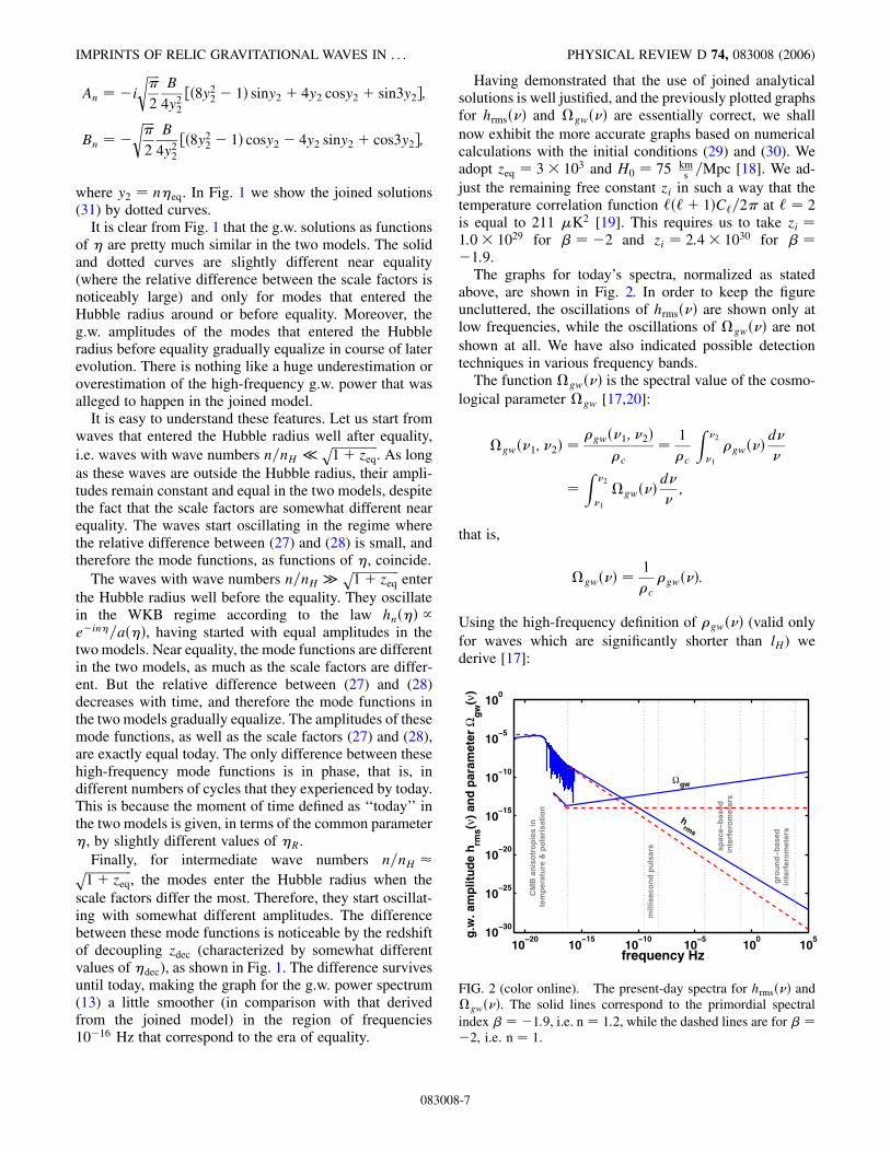
Having demonstrated that the use of joined analyticalsolutions is well justified, and the previously plotted graphsfor hrms and gw are essentially correct, we shallnow exhibit the more accurate graphs based on numericalcalculations with the initial conditions (29) and (30). Weadopt zeq 3 103 and H0 75 km

s =Mpc [18]. We ad-just the remaining free constant zi in such a way that thetemperature correlation function ‘‘ 1C‘=2 at ‘ 2is equal to 211 K2 [19]. This requires us to take zi 1:0 1029 for 2 and zi 2:4 1030 for 1:9.

The graphs for today’s spectra, normalized as statedabove, are shown in Fig. 2. In order to keep the figureuncluttered, the oscillations of hrms are shown only atlow frequencies, while the oscillations of gw are notshown at all. We have also indicated possible detectiontechniques in various frequency bands.

The function gw is the spectral value of the cosmo-logical parameter gw [17,20]:

gw1; 2 gw1; 2

c

1

c

Z 2

1

gwd

Z 2

1

gwd;

that is,

gw 1

cgw:

Using the high-frequency definition of gw (valid onlyfor waves which are significantly shorter than lH) wederive [17]:

10−20

10−15

10−10

10−5

100

105

10−30

10−25

10−20

10−15

10−10

10−5

100

frequency Hz

g.w

. am

plit

ud

e h rm

s(ν)

and

par

amet

er Ω

gw

(ν)

sp

ace−

bas

ed

inte

rfer

om

eter

s

gro

un

d−b

ased

inte

rfer

om

eter

s

mill

isec

on

d p

uls

ars

C

MB

an

iso

tro

pie

s in

tem

per

atu

re &

po

lari

sati

on

hrms

Ωgw

FIG. 2 (color online). The present-day spectra for hrms andgw. The solid lines correspond to the primordial spectralindex 1:9, i.e. n 1:2, while the dashed lines are for 2, i.e. n 1.


083008-7

gw 2

3h2

rmsH

2: (32)

It is this definition of gw that is used for drawing thecurves in Fig. 2.

We have to warn the reader that a great deal of literatureon stochastic g.w. backgrounds uses the incorrect defini-tion

gw 1

c

dgw

d ln;

which suggests that the gw parameter is zero if theg.w. spectral energy density gw is frequency-independent, regardless of the numerical value of gw.Then, from this incorrect definition, a formula similar toEq. (32) is often being derived by making further compen-sating errors.

The higher-frequency part of hrms is relevant fordirect searches for relic gravitational waves, while thelower-frequency part is relevant to the CMB calculationsthat we turn to in the next section. The direct and indirectmethods of detecting relic gravitational waves are consid-ered in a large number of papers (see, for example, [5,20–28] even though we disagree with some of them).

It is important to keep in mind that according to theinflationary theory the dashed lines for gw and hrmsin Fig. 2 should be at a zero level, because they describe theg.w. background with a flat primordial spectrum 2,n 1. The ‘‘consistency relation’’ of the inflationary the-ory demands r 0, i.e. vanishingly small g.w. back-ground, in the limit n 1.

III. EQUATIONS OF RADIATIVE TRANSFER

A. Characterization of a radiation field

The radiation field is usually characterized by the fourStokes parameters I; Q;U; V, [29,30]. The parameter I isthe total intensity of radiation, Q and U describe themagnitude and direction of linear polarization, and V isthe circular polarization. The Stokes parameters can beviewed as functions of photons’ coordinates and momentax; p. Since photons propagate with the speed of light c,the momenta satisfy the condition pp 0. Thus, theStokes parameters are functions of t; xi; ; ei, where isthe photon’s frequency, and ei is a unit vector in thedirection of observation (opposite to the photon’spropagation).

In a given space-time point t; xi, the Stokes parametersare functions of , , , where , are coordinates on aunit sphere:

d2 gabdxadxb d2 sin2d2: (33)

The radial direction is the direction of observation.The Stokes parameters are components of the polariza-

tion tensor Pab [30] which can be written as

Pab; 1

2I Q U iV sin

U iV sin I Qsin2

:

(34)

(We do not indicate the dependence of Stokes parameterson .)

The symmetry of Pab with respect to rotations aroundthe direction of observation requires the vanishing of linearpolarization Q 0, U 0, but the circular polarization Vcan be present. The symmetry of Pab with respect tocoordinate reflections in the observation plane requiresV 0, but the linear polarization can be present. The firstsymmetry means that the readings of a linear polarimeterare the same when it is rotated in the observation plane.The second symmetry means that the readings of the left-handed and right-handed circular polarimeters are thesame. (Compare with the discussion on gravitational wavesin Sec. II A.)

Under arbitrary transformations of ,, the componentsof Pab; transform as components of a tensor, but somequantities remain invariant. We want to build linear invar-iants from Pab and its derivatives, using the metric tensorgab; and a completely antisymmetric pseudotensorab;,

ab 0 sin1

sin1 0

:

The first two invariants are easy to build:

I; gab;Pab;;

V; iab;Pab;:(35)

Then, it is convenient to single out the trace and antisym-metric parts of Pab, and introduce the symmetric trace-free(STF) part PSTF

ab :

Pab; 1

2Igab

i2Vab P

STFab ;

PSTFab

1

2

Q U sin

U sin Qsin2

!:

Clearly, the construction of other linear invariants re-quires the use of covariant derivatives of the tensor PSTF

ab .There is no invariants that can be built from the firstderivatives PSTF

ab;c, so we need to go to the second deriva-tives. One can check that there are only two linearlyindependent invariants that can be built from the secondderivatives:

E; 2PSTFab

;a;b; B; 2PSTFab

;b;dad;

(36)

The quantities I and E are scalars, while V and B arepseudoscalars. V and B change sign under flips of direc-tions (coordinate transformations with negative determi-nants). This is also seen from the fact that theirconstruction involves the pseudotensor ab.


083008-8

The invariant quantities I; V; E; B, as functions of ,,can be expanded over ordinary spherical harmonicsY‘m;, Y ‘m 1mY‘;m:

I; X1‘0

X‘m‘

aT‘mY‘m;; (37a)

V; X1‘0

X‘m‘

aV‘mY‘m;; (37b)

E; X1‘2

X‘m‘

‘ 2!

‘ 2!

1=2aE‘mY‘m;; (37c)

B; X1‘2

X‘m‘

‘ 2!

‘ 2!

1=2aB‘mY‘m;: (37d)

The set of multipole coefficients aT‘m; aV‘m; a

E‘m; a

B‘m com-

pletely characterizes the radiation field. We will use thesequantities in our further discussion.

To make contact with previous work, we note that themultipole coefficients aE‘m, aB‘m can also be expressed interms of the tensor Pab itself, rather than its derivatives.This is possible because one can interchange the order ofdifferentiation under the integrals that define aE‘m, aB‘m interms of the right-hand side (r.h.s.) of Eq. (36). This leadsto the appearance of the spin-weighted spherical harmonicsor tensor spherical harmonics [12–14,31,32]. For example,the tensor Pab can be written as

Pab 1

2

X1‘0

X‘m‘

gabaT‘m iaba

V‘mY‘m;

12p

X1‘2

Xlml

aE‘mYG‘mab;

aB‘mYC‘mab;;

where YG‘mab; and YC

‘mab; are the ‘‘gradient’’and ‘‘curl’’ tensor spherical harmonics forming a set oforthonormal functions for STF tensors [32]. The invariantsE and B can also be written in terms of the spin raising andlowering operators ð and ð [31]:

E 1

2ð2Q iU ð2Q iU;

B i2ð2Q iU ð2Q iU:

The quantities E and B are called the E (or gradient) andB (or curl) modes of polarization. The ‘-dependent nu-merical coefficients in (37c) and (37d) were introduced inorder to make the definitions of this paper fully consistentwith the previous literature [31,32].

B. Radiative transfer in a perturbed universe

We need to work out the radiative transfer equation in aslightly perturbed universe described by Eq. (1). The

Thompson scattering of initially unpolarized light cannotgenerate circular polarization, so we shall not consider theV Stokes parameter. Following [29,33,34], we shall writethe radiative transfer equation in terms of a 3-componentquantity (symbolic vector) nx; p. The componentsn1; n2; n3 are related to the Stokes parameters by

n n1

n2

n3

0@ 1A 1

2

c2

h3

I QI Q2U

0@ 1A; (38)

where h is the Planck constant. The quantities n1, n2, n1 n2 n3=2 are the numbers of photons of frequency coming from the direction z and passing through a slitoriented, respectively, in the directions x, y, and the bisect-ing direction between x and y.

The equation of radiative transfer can be treated as aBoltzmann equation in a phase space. The general form ofthis equation is as follows [35]

Dnds Cn; (39)

where s is a parameter along the worldline of a photon, Dds isa total derivative along this worldline, and C is a collisionterm. We shall explain each term of this equationseparately.

The total derivative in Eq. (39) reads:

Dnds

dx

ds@@xdp

ds@@p

n; (40)

where dx=ds and dp=ds are determined by the lightlikegeodesic worldline,

dx

ds p;

dp

ds p

p ; gpp 0:

(41)

Strictly speaking, the square bracket in Eq. (40) should alsoinclude the additive matrix term R. This term is respon-sible for the rotation of polarization axes that may takeplace in course of parallel transport along the photon’sgeodesic line [36]. In the perturbation theory that we areworking with, this matrix does not enter the equations inthe zeroth and first-order approximations [33], and there-fore we neglect R.

In our problem, the collision term C describes theThompson scattering of light on free (not combined inatoms) electrons [29]. We assume that the electrons areat rest with respect to one of synchronous coordinatesystems (1). We work with this coordinate system, so thatit is not only synchronous but also ‘‘comoving’’ with theelectrons. (This choice is always possible when the func-tions hij in (1) are gravitational waves. Certain complica-tions in the case of density perturbations will be consideredlater, Appendix D.) Thus, the collision term C is given bythe expression


083008-9

Cn TNexcdtds

nt; xi; ; ;

1

4

Zd0P;; 0; 0nt; xi; ; 0; 0

; (42)

where T 6:65 1024 cm2 is the Thompson cross sec-tion, Ne is the density of free electrons, and P;; 0; 0is the Chandrasekhar scattering matrix. (The explicit formof the scattering matrix is discussed in Appendix C.) Thefactor cdt=ds arises because of our use of the element ds,instead of cdt, in the left-hand side (l.h.s.) of Eq. (39). Inaccord with the meaning of the scattering term, the quan-tity TNexcdt=ds is the averaged number of electronsthat could participate in the scattering process when thephoton traversed the element ds along its path.

Let us now write down the equations of radiative transferin the presence of the gravitational field (1). First, we writedown the equations for the lightlike geodesic line xs s; xis:

p0 dds

ca; pi

dxi

ds

caei;

dds

1

adad

1

2eiej

@hij@

dds;

ij hijeiej 1:

(43)

We do not need the expression for dei=ds, because it is afirst-order (in terms of metric perturbations) quantity, andthis quantity enters the equations of radiative transfer onlyin products with other first-order terms. We neglect suchsecond-order corrections.

Second, we write for the ‘‘vector’’ n:

n n0 n1; (44)

where n0 is the zeroth order solution, and n1 is the first-order correction arising because of the presence of metricperturbations. We shall now formulate the equation forn1, taking into account the zero-order solution to Eq. (39).

In the zero-order approximation we assume that hij 0and that the radiation field is fully homogeneous, isotropic,and unpolarized. Therefore,

n 0 n0; u; (45)

where

u 110

0@ 1A:Since the scattering matrix P does not couple to theradiation field if it has no quadrupole anisotropy, thecollision term (42) vanishes, Cn0 0, and the equationfor n0; reads

@n0

@adad

@n0

@ 0:

The general solution to this equation is n0 n0a,which makes it convenient to use a new variable

~ a:

In the zero-order approximation, const=a andtherefore ~ is a constant along the light ray.

We are now in a position to write down the first-orderapproximation to the Boltzmann Eq. (39). We take; xi; ~; ei as independent variables, i.e. n0 n0~,n1 n1; xi; ~; ei, and use the identity

dp

ds

@@p

d~ds

@@~dei

ds@@ei

in the first-order approximation to (40). Taking also intoaccount the geodesic Eq. (43) we arrive at the equation

@n1

@ ei

@n1

@xi

1

2~eiej

@hij@

@n0

@~

dds Cn1:

Introducing new notations q TaNe andf~ @ lnn0=@ ln~ [33] (the astrophysical meaning andnumerical values of the functions q and f~ are dis-cussed in Appendix B) we write down the final form of thetransfer equation:

@@ q ei

@@xi

n1; xi; ~; ei

f~n0~

2eiej

@hij@

u q1

4

Zd0Pei; e0jn1; xi; ~; e0j: (46)

It is seen from Eq. (46) that the ‘‘source’’ for thegeneration of n1 consists of two terms on the r.h.s. ofthis equation. First, it is the gravitational-field perturbationhij, participating in the combination eiej@hij=@. It di-rectly generates a structure proportional to u, i.e. a varia-tion in the I Stokes parameter and a temperatureanisotropy. In this process, a quadrupole component ofthe temperature anisotropy necessarily arises due to thepresence of the term ei@=@xi, even if the above-mentionedcombination itself does not have angular dependence. Thesecond term on the r.h.s. of Eq. (46) generates polarization,i.e. a structure different from u. This happens because ofthe mixing of different components of n1, including thoseproportional to u, in the product term Pn1. In other words,polarization is generated by the scattering of anisotropicradiation field. Clearly, polarization is generated only inthe intervals of time when q 0, i.e. when free elec-trons are available for the Thompson scattering (see, forexample, [37]).


083008-10

C. The radiative transfer equations for a single gravitational wave

We work with a random gravitational field hij expanded over spatial Fourier components (10). It is convenient to makesimilar expansion for the quantities n1; xi; ~; ei. Since Eq. (46) is linear, the Fourier components of n1 inherit thesame random coefficients c

sn that enter Eq. (10):

n 1; xi; ~; ei C

23=2

Z 11

d3n2np

Xs1;2

n1n;s; ~; eieinxcs

n n1 n;s ; ~; eieinxcs

n: (47)

Equation (46) for a particular Fourier component takes the form:

@@ q ieini

n1n;s; ~; ei

f~n0~2

eiejpsijn

dhs

nd

uq4

Zd0Pei; e0jn1n;s; ~; e0j: (48)

To simplify technical details, we start with a singlegravitational wave propagating exactly in the direction ofz in terms of definitions (2), (4), and (19). The coordinatesystem, associated with the wave, is specified by 0, 0. This simplifies the polarization tensors (19) andmakes them constant matrices. At the same time, theobservation direction is arbitrary and is defined by ei sin cos; sin sin; cos. We consider circularly polar-ized states with s 1 L, s 2 R. Then, we find

eiejpsijn 12e2i; (49)

where cos and the signs correspond to s L, R,respectively. This simplification of the angular dependenceis possible only for one Fourier component, but not for allof them together. We shall still need the results for a wavepropagating in an arbitrary direction. The necessary gen-eralization will be done in Sec. V B.

The 2 angular dependence of the source term inEq. (48) generates the 2 angular dependence in thesolution [33,34]. We show in Appendix C that the terms inn1n;s; ~;; with any other -dependence satisfy ho-mogeneous differential equations, and therefore they van-ish if they were not present initially (which we alwaysassume). Similarly, the ~ dependence of the solution can befactored out. Finally, we show in Appendix C that onelinear combination of the three components of n1n alwayssatisfies a homogeneous equation and therefore vanishes atzero initial data. Thus, the problem of solving Eq. (48)reduces to the problem of finding two functions of thearguments , .

Explicitly, we can now write

n 1n;s; ~;; f~n0~

2

264n;s;12

110

0@

1A

n;s;12

12

4i

0B@

1CA375e2i:

(50)

Clearly, function is responsible for temperature anisot-ropy (I Stokes parameter), while function is responsiblefor polarization (Q and U Stokes parameters).

Temporarily dropping out the labels n, s and introducingthe auxiliary function ; ; ;, weget from Eqs. (48) and (50) a pair of coupled equations[34]:

@;@

q in; 3

16qI;

(51)

@;@

q in; dhd

; (52)

where

I Z 1

1d0

1022;0

1

21022;0

: (53)

IV. RADIATIVE TRANSFER EQUATIONS AS ASINGLE INTEGRAL EQUATION

In some previous studies [31,38,39], Eqs. (51) and (52)are being solved by first expanding the -dependence interms of Legendre polynomials. This generates an infiniteseries of coupled ordinary differential equations. Then, theseries is being truncated at some order.

We go by a different road. We demonstrate that theproblem can be reduced to a single mathematically con-sistent integral equation. There are technical and interpre-tational advantages in this approach. The integral equationenables us to derive physically transparent analytical solu-tions and make reliable estimates of the generated polar-ization. The numerical implementation of the integralequation considerably saves computing time and allowssimple control of accuracy.


083008-11

A. Derivation of the integral equation

In order to show that the solutions of Eqs. (51) and (52)for ; and ; are completely determined by asingle integral equation, we first introduce new quantities[40]

3

16gI; (54)

H edhd

: (55)

Solutions to Eqs. (51) and (52) can be written as

; einZ

0d00ein

0; (56)

; einZ

0d0H0ein

0; (57)

Expression (56) is a formal solution to Eq. (51) in the sensethat ; is expressed in terms of which itselfdepends on ; (see (53) and (54)).

We now put (56) and (57) into Eq. (53) to get a newformulation for I:

I eZ 1

1

Z

0dd0

1220

1

2122H0

ein

0: (58)

Using the kernels K 0,

K 0

Z 1

1d122ein

0; (59)

Equation (58) can be rewritten as

I eZ

0d0

K

00

1

2K 0H0

: (60)

Multiplying both sides of this equality by3=16qe and recalling the definition (54) we ar-rive at a closed form equation for :

3

16q

Z

0d00K 0 F;

(61)

where F is the known gravitational-field term given bythe metric perturbations,

F 3

32q

Z

0d0H0K

0; (62)

The derived Eq. (61) for is the integral equation ofVoltairre type. As soon as is found from this equa-tion, we can find ; from Eq. (56). Then, Eqs. (56)

and (57) completely determine all the components of n1

according to Eq. (50).Clearly, we are mainly interested in temperature and

polarization anisotropies seen at the present time R. Introducing nR and restoring the indicesn and s, we obtain the present-day values of and :

n;s n;sR; Z R

0dHn;sn;sei ;

(63a)

n;s n;sR; Z R

0dn;sei : (63b)

The integrals can safely be taken from 0 as the opticaldepth quickly becomes very large in the early Universe,and the source functions Hn;s and n;s quicklyvanish there. We will work with expressions (63) in ourfurther calculations.

B. Analytical solution to the integral equation

The integral Eq. (61) can be solved analytically in theform of a series expansion. Although our graphs andphysical conclusions in this paper are based on the exactnumerical solution to Eq. (61), it is important to have asimple analytical approximation to the exact numericalsolution. We will show below why the infinite series canbe accurately approximated by its first term and how thissimplification helps in physical understanding of the de-rived numerical results.

We start with the transformation of kernels (59) ofthe integral Eq. (61). Using the identity keix d=idxkeix, the kernels can be written as

K 0 Z 1

1d122ein

0

21

d2

dx2

2 sinxx;

where x n 0. Now, taking into account the expan-sion

sinxx

X1m0

1m

2m 1!x2m;

the r.h.s. of Eq. (61) can be presented in the form of aseries:

3

2q

X1m0

n2mZ

0d0 02m

m0 mH

0; (64)

where


083008-12

m 1m

2m 1!

1 4

m 2

2m 32m 5

;

m 1m

2m 1!2m 32m 5:

Since the r.h.s. of Eq. (64) is a series in even powers ofthe wave number n, the l.h.s. of the same equation can also

be expanded in powers of n2m:

X1m0

mn2m: (65)

Using expansion (65) in both sides of Eq. (64) we trans-form this equation to

X1m0

mn2m 3

2q

"X1m0

X1j0

mn2mjZ

0d0j0 02m

X1m0

mn2mZ

0d0H0 02m

#:

(66)

The left side and the second term in the right side of Eq. (66) are series in n2m, but the first sum on the r.h.s. of Eq. (66) isstill a mixture of different powers. This sum can be rearranged to be manifestly a series in n2m:

X1m0

X1j0

mn2mjZ

0d0j0 02m

X1m0

n2m

"Xmk0

kZ

0d0mk0 02k

#: (67)

According to Eq. (66) we have to make equal the co-efficients of terms with the same power n2m in both sides ofthe equation. This produces a set of integral equations

m qSm 7

10q

Z

0d0m0;

(68)

where functions Sm depend only on the known func-tion H and functions mk presumed to be foundfrom equations of previous orders:

Sm 3

2m

Z

0d0H0 02m

3

2

Xmk1

kZ

0d0mk0 02k:

(69)

The important advantage of the performed expansion inpowers of n2m is that Eq. (68) of any order m is now a self-contained analytically solvable integral equation.

Exact solution to the integral Eq. (68) is given by theformula

m qZ

0d0

dSm0d0

e7=10;0: (70)

We can further simplify this formula. Taking an-derivative of expression (69) we find

dSmd

1

10H0m !m

Z

0d0H0 02m1

Xmk1

!kZ

0d0mk0 02k1;

where !m 3mk. Substituting this expressioninto Eq. (70), we arrive at the final result

m qe7=10Z

0d0e7=100

H0

1

100m !mm;0

Xmk1

!kmk0k;0; (71)

where

k;0 Z

0d00e7=1000;000 02k1: (72)

Functions k;0 depend only on the ionizationhistory of the background cosmological model describedby q. These functions can be computed in advance.Complete determination of the function , Eq. (65),requires only one integration by at each level m inEq. (71), starting from m 0. The zero-order term0 does not depend on functions k and is deter-mined exclusively by H, Eq. (55). The zero-order termcan be presented as


083008-13

0n 1

10g

Z

0d0

dhn0d

e3=10;0: (73)

It is crucial to remember that the function ,Eq. (54), always contains the narrow visibility functiong (see Appendix B). In particular, function 0 isnonzero only for within the width of g, and isproportional to this width. In the era of decoupling, wedenote the characteristic width of g by dec. Withdec we associate the characteristic wave number n :

n 2

dec:

Numerically, dec 3 103 and n 2 103. Inwhat follows, we will be interested in CMB multipoles ‘ &

103. They are mostly generated by perturbations with wavenumbers n & 103. Therefore, for wave numbers of interest,we regard n=n as a small parameter.

We shall now show that 0 is the dominant term ofthe series (65). The next term, 1n2, is at least a factorn=n 2 smaller than 0, and so on. The explicitexpression for 1 is as follows

1 gZ

0d0

!1

dh0d0

!1e000

e3=10;01;0:

Effectively, function 1, in comparison with 0,contains an extra factor 1;

0. Taking into accountthe fact that the functions g and e7=1000;0 arelocalized in the interval of arguments not larger thandec, this factor evaluates to a number not larger thandec

2. Therefore, them 1 term in Eq. (65) is at least afactor n=n 2 smaller than the m 0 term.

These analytical evaluations are confirmed by numericalanalysis as shown in Fig. 3. The solid line shows the exactnumerical solution found from Eq. (61) for hn and qdescribed in Sec. II B and Appendix B respectively. Thedashed line is plotted according to formula (73), with thesame hn and q. It is seen from Fig. 3 that the zero-order term 0 is a good approximation. The deviationsare significant, they reach (20–25)%, only for the largestwave numbers n in the domain of our interest.

V. MULTIPOLE EXPANSION AND POWERSPECTRA OF THE RADIATION FIELD

A. Multipole coefficients

Having found n;s for a single gravitational wavespecified by Eq. (49) one can find and functionsaccording to Eqs. (63a) and (63b). Then, usingEqs. (34)–(36), (38), and (50), one can find the multipolecoefficients aX‘m X I; E; B participating in the decom-positions (37). Although this route has been traversedbefore [31], we have made independent calculations in a

0.01 0.015 0.02 0.025 0.03 0.035 0.04

0

0.5

1

1.5

time η

Φ(η

)

n = 100

0.01 0.015 0.02 0.025 0.03 0.035 0.04−0.1

0

0.1

0.2

0.3

0.4

time η

Φ(η

)

n = 500

0.01 0.015 0.02 0.025 0.03 0.035 0.04−0.25

−0.2

−0.15

−0.1

−0.05

0

0.05

0.1

0.15

time η

Φ(η

)

n = 1000

0.01 0.015 0.02 0.025 0.03 0.035 0.04−0.2

−0.15

−0.1

−0.05

0

0.05

0.1

0.15

time η

Φ(η

)

n = 1500

FIG. 3 (color online). Function n for different values of n. The solid line is exact numerical solution to Eq. (61). The dashed lineis the zero-order approximation (73). The dotted line shows the approximation (91) (see below). The g.w. mode functions arenormalized such that hnr 1.


083008-14

more general arrangement. Formulas derived in this subsection are effectively a confirmation of the correctness ofcalculations in Ref. [31].

First, we integrate over photon frequencies (for the definition of see Eq. (B3)) and arrive at the following expressions

In;s; 12n;se2i; (74a)

En;s; 12

12

d2

d2 8dd 12

n;se

2i; (74b)

Bn;s;

212

i

d2

d2 4idd

n;se2i

; (74c)

where, as before, the upper and lower signs correspond tos 1 L and s 2 R, respectively. The 2 depen-dence in Eqs. (74) implies that only the m 2 multi-poles are nonzero.

Then, we integrate Eqs. (74) over angular variables inorder to find aX‘m according to Eq. (37). Using the notationsT‘, E‘, B‘ for the functions arising in course ofcalculations (and called multipole projection functions)

T‘

‘ 2!

‘ 2!

sj‘

2 ; (75a)

E‘

2ll 1

2

j‘

2

j‘1

; (75b)

B‘ 2‘ 1

j‘ j‘1

; (75c)

and replacing and by their expressions (63), wefinally arrive at

aT‘mn; s i‘22;m1;s 2;m2;saT‘ n; s; (76a)

aE‘mn; s i‘22;m1;s 2;m2;saE‘ n; s; (76b)

aB‘mn; s i‘22;m1;s 2;m2;sa

B‘ n; s; (76c)

where

aT‘ n;s 42‘ 1

p Z R

0dHn;sn;sT‘;

(77a)

aE‘ n;s 42‘ 1

p Z R

0dn;sE‘; (77b)

aB‘ n;s 42‘ 1

p Z R

0dn;sB‘: (77c)

B. Superposition of gravitational waves with arbitrarywave vectors

It is important to remember that the result (76) is validonly for a special wave, with the wave vector n orientedexactly along the coordinate axis z. Since the perturbedgravitational field is a random collection of waves with allpossible wave vectors n, and we are interested in theirsummarized effect as seen in some fixed observational

direction , , we have to find the generalization ofEq. (76) to an arbitrary wave, and then to sum them up.

To find the effect of an arbitrary wave, there is no need todo new calculations. It is convenient to treat calculations inSec. VA as done in a (primed) coordinate system speciallyadjusted to a given wave in such a manner that the wavepropagates along z0, n0 0; 0; n. The observational di-rection ei is characterized by 0, 0. The quantities X I,E, B calculated in Sec. VA are functions of 0, 0 ex-panded over Y‘m0; 0,

Xn0;s;0 X1‘0

X‘m‘

aX‘mn; sY‘m0; 0; (78)

where aX‘m is a set of coefficients (compare with Eq. (37)):aT‘m, ‘ 2!=‘ 2!1=2aE‘m, ‘ 2!=‘ 2!1=2aB‘m.

Now, imagine that this special (primed) coordinate sys-tem is rotated with respect to the observer’s (unprimed)coordinate system by some Euler angles

n; n; 0

(see, for example [41]). The same observational directionei is now characterized by , , and the same wave vectorn0 is now characterized by the unit vector

~n n=n sinn cosn; sinn sinn; cosn:

Obviously, the already calculated numerical values of theinvariants X0; 0 do not depend on the rotation of thecoordinate system. Being expressed in terms of , , theinvariants describe the effect produced by a wave with agiven (arbitrary) unit wave vector ~n, as seen in the direc-tion , .

The transformation between coordinate systems 0; 0and ; is accompanied by the transformation of spheri-cal harmonics,

Y‘m0; 0 X‘

m0‘

D‘m0;m~nY‘m0 ;;

where

D‘m0;m~n D‘

m0;mn; n; 0

are the Wigner symbols [42]. Later, we will need theirorthogonality relationship


083008-15

ZdD‘

m;p~nD‘0 m0;p~n

42‘ 1

‘‘0mm0 ; (79)

where d sinndndn.We can now rewrite Eq. (78) in terms of , , and thus

find the contribution of a single arbitrary Fourier compo-nent,

Xn;s; X1‘0

X‘m‘

X‘m0‘

aX‘m0 n; sD‘mm0 ~n

!Y‘m;:

(80)

The superposition of all Fourier components of the per-turbed gravitational field gives, at the observer’s positionx 0 and at R (see (47)), the final result:

X; C

23=2

Z 11

d3n2np

Xs1;2

Xn;s;cs

n X n;s;cs

n: (81)

From this expression, combined with Eq. (80), one canread off the random multipole coefficients aX‘m that partici-pate in the expansions (37):

aX‘m C

23=2

Z 11

d3n2np

Xs1;2

X‘m0‘

aX‘m0 n; sD‘m;m0 ~nc

sn

1maX ‘m0 n; sD‘ m;m0 ~nc

s

n: (82)

Since X is a real field, the multipole coefficients aX‘m obeythe reality conditions

aX ‘m 1maX‘;m; (83)

as is seen directly from (82). The gravitational-wave nature

of metric perturbations is encoded in concrete values of thecoefficients (37) and (77). But in all other aspects theargumentation presented here is general.

C. Angular power spectra for temperatureand polarization anisotropies

It follows from Eq. (82) that the statistical properties ofthe multipole coefficients aX‘m are fully determined by thestatistical properties of the gravitational-field perturbationsrepresented by the random coefficients c

sn. A particular

realization of cs

n is responsible for the particular realizationof aX‘m actually observed in the sky. Having derived thedistribution function for c

sn from some fundamental con-

siderations (for example, from the assumption of the initialquantum-mechanical vacuum state of perturbations) wecould estimate the probability of the observed set aX‘mwithin the ensemble of all possible sets. We could alsoevaluate the inevitable uncertainty in the observationaldetermination of the parameters of the underlying randomprocess. This uncertainty is associated with the inherentabsence of ergodicity of any random process on a 2-sphere(i.e. sky) [43]. In this paper, however, we adopt a minimal-istic approach; we postulate only the relationships (16) andcalculate only the quadratic correlation functions for aX‘m.

Clearly, the mean values of the multipole coefficients arezeros,

haX‘mi haX‘m i 0:

To calculate the variances and cross-correlation functions,we have to form the products aX ‘ma

X0‘0m0 and then take their

statistical averages. First, we find

haX ‘maX0‘0m0 i

C2

23Z n2dnd

2n

Xs1;2

X‘m1‘

X‘m01‘

aX ‘m1n; saX

0

‘0m01n; sD‘

mm1~nD‘0

m0m01~n

aX‘m1n; saX

0 ‘0m01n; sD‘

m;m1~nD‘0

m0;m01~n: (84)

We now take into account the fact (compare withEq. (76)) that

aX‘m1n; saX

0

‘0m01n; s / m1m01

:

This property allows us to get rid of summation over m01 inEq. (84). Then, we perform integration over d and usethe orthogonality relationships (79). We finally arrive at

haX ‘maX0‘0m0 i CXX

0

‘ ‘‘0mm0 ; (85)

where

CXX0

‘ C2

422‘ 1

Zndn

Xs1;2

X‘m‘

aX‘mn; saX0 ‘m n; s

aX ‘mn; saX0‘mn; s: (86)

Other quadratic averages, such as haX‘maX0‘0m0 i, ha

X ‘ma

X0 ‘0m0 i,

follow from (85) and the reality condition (83).The angular correlation and cross-correlation functions

of the fields I, E, B are directly expressible in terms ofEq. (86). For example,

hI1; 1I2; 2i X1‘0

2‘ 1

4CTT‘ P‘cos;


083008-16

where is the angular separation between the directions1; 1 and 2; 2 on the sky. If the actually measuredvalues of aX‘m represent a particular realization of aGaussian random process, quantities CXX

0

‘ , constructedfrom the measured aX‘m according to the r.h.s. of Eq. (86),are the best unbiased estimates [43].

One can note that the final result (85) and (86) is theintegral of individual contributions (76) from single gravi-tational waves given in a special frame discussed inSec. VA. However, one cannot jump directly from (76)to (86) (which is often done in the literature). In general,Eq. (86) does not follow from Eq. (76). By calculationsgiven in this subsection we have rigorously shown thatEq. (86) is justified only if special statistical assumptions(16) are adopted.

One can also note that the correlation functions contain-ing the label B once, i.e. CTB‘ and CEB‘ , vanish if the extraassumptions (18) and (23) are made. Indeed, under theseassumptions one can use one and the same mode functionfor both polarization states s, Eq. (24). Then, the coeffi-cients aB‘mn; s, Eq. (76c), differ essentially only in signfor two different s, i.e. aB‘2n; L a

B‘;2n; R. There-

fore, their contributions will cancel out in expressions (86)for CTB‘ and CEB‘ . This statement is in agreement withRef. [44].

Without having access to a theory of everything whichcould predict one unique distribution of the CMB radiationfield over the sky, we have to rely on the calculatedstatistical averages (86). We can also hope that our uni-verse is a ‘‘typical’’ one, so that the observed values of thecorrelation functions should not deviate too much from thestatistical mean values.

VI. EFFECTS OF RECOMBINATION ERA

All our final graphs and physical conclusions in thispaper are based on exact formulas and numerical calcula-tions, starting from numerical representation of the keyfunctionsH and , Eqs. (55) and (61). However, wederive and explain all our results by developing manage-able and accurate analytical approximations. At every level

of calculations we compare exact numerical results withanalytical ones.

A. Temperature anisotropy angular power spectrum

The temperature anisotropy power spectrum CTT‘ is de-termined by the multipole coefficients aT‘ n; s, Eqs. (86),(76a), and (77a). The typical graphs for the functionsHn;s and n;s are shown in Fig. 4.

Since the visibility function g is a narrow function, aconvenient analytical approximation is the limit of aninstantaneous recombination. The function e is replacedby a step function changing from 0 to 1 at dec, e h dec, and the function g is replaced by a delta-function, g dec. In this limit, the contribu-tion to aT‘ n; s from the scattering term 0n;s is propor-tional to dec. It can be neglected in comparison with thecontribution from the gravitational term Hn;s. The ratioof these contributions is of the order of nrec, and it tendsto zero in the limit of instantaneous recombination,dec ! 0.

Neglecting the scattering term, we write

aT‘ n; s 42‘ 1

p Z R

dec

ddhs

n

dT‘: (87)

This integral can be taken by parts,

aT‘ n; s 42‘ 1

p h

s

ndecT‘dec

Z R

dec

dnhs

ndT‘d

:

The remaining integral contains oscillating functions andits value is smaller, for sufficiently large n’s, than the valueof the integrated term. This is illustrated in Fig. 5.Therefore, we have

aT‘ n; s 42‘ 1

phs

ndecT‘dec: (88)

Finally, we put Eq. (88) into Eq. (86) and take intoaccount the definition of the metric power spectrum (13).Then, we get

0 0.2 0.4 0.6 0.8 1−40

−30

−20

−10

0

10

20

time η

Hn(η

)

0 0.02 0.04 0.06 0.08 0.1−0.5

0

0.5

1

1.5

time η

Φn( η

)

FIG. 4 (color online). The source functions Hn;s and n;s (n 100) of temperature and polarization anisotropies (thenormalization is chosen such that hnr 1).


083008-17

CTT‘ 4 2Z dn

nh2n; decT

2‘dec: (89)

The projection factor T2‘dec is given by Eq. (75a).

Since the spherical Bessel functions reach maximumwhen the argument and the index are approximately equal,dec ‘, a particular wave number n is predominantlyprojected onto the multipole ‘ n:

‘ dec nR dec n: (90)

This can also be seen in Fig. 5. Thus, the oscillatoryfeatures of the metric power spectrum h2n; dec in then-space are fully responsible for the oscillatory features ofthe angular power spectrum ‘‘ 1CTT‘ in the ‘-space[11]. (We use this opportunity to correct a misprint in Fig. 2of Ref. [11]: the plotted lines are functions Cl, not ll1Cl. For the early graphs of C‘ see Ref. [45].)

The g.w. metric power spectrum h2n; dec for the case 2, and the function ‘‘ 1CTT‘ caused by thisspectrum, are shown in Fig. 7(b) and 7(a). The normaliza-tion of the metric power spectrum is such that the function‘‘ 1CTT‘ at ‘ 2 is equal to 1326 K2 [19]. Theinterval ‘ & 90 is generated by waves with n & 90.These waves did not enter the Hubble radius by the timedec. Their amplitudes are approximately equal for all n’sin this interval (compare with Fig. 1). The gradual decreaseof the angular power spectrum at larger ‘’s is the reflectionof the gradual decrease of power in shorter gravitationalwaves whose amplitudes have been adiabatically decreas-

ing since the earlier times when the waves entered theHubble radius.

B. Polarization anisotropy angular power spectrum

The decisive function for polarization calculations isn;s. We have approximated this function by 0n;s,Eq. (73), and compared it with exact result in Fig. 3. Forqualitative derivations it is useful to make furthersimplifications.

Since g is a narrow function, the integral in Eq. (73)is effective only within a narrow interval dec. Assuming

that the function dhs

n=d does not vary significantlywithin this interval, we can take this function from underthe integral,

0n;s 1

10

dhs

nd

g

Z

0d0e3=10;0

:

(91)

Clearly, the assumption that the function dhs

n=d isalmost constant within the window dec gets violatedfor sufficiently short waves. With (91), we expect degra-dation of accuracy for wave numbers n approaching n .This is illustrated by a dotted line in Fig. 3. Nevertheless,the approximation (91) is robust for n & n , and it revealsthe importance of first derivatives of metric perturbationsfor evaluation of the CMB polarization.

We now introduce the symbol P to denote either E or Bcomponents of polarization. In terms of multipoles

0 5 10 15 200

0.05

0.1

0.15

0.2

0.25

0.3

0.35

0.4

0.45

multipole l

l(l+

1)C

l

n = 10

0 10 20 30 40 50 60 700

0.2

0.4

0.6

0.8

1

multipole l

l(l+

1)C

l

n = 50

0 50 100 1500

0.1

0.2

0.3

0.4

0.5

multipole l

l(l+

1)C

l

n = 100

0 100 200 300 400 500 600 7000

0.5

1

1.5

2

2.5x 10

−3

multipole l

l(l+

1)C

l

n = 500

FIG. 5 (color online). The contributions to the power spectrum ‘‘ 1CTT‘ from an individual mode n. The solid line shows theexact result calculated according to (87), while the dashed line shows the approximation (88). The normalization has been chosen suchthat hnr 1.


083008-18

aP‘ n; s, the angular power spectrum is given by Eq. (86).Putting (91) into Eqs. (77b) and (77c) and denoting byP‘ the respective projection functions, we get

aP‘ n; s 42‘ 1

p Z R

0d

1

10

dshnd

P‘

g

Z

0d0e3=10;0

: (92)

Again referring to the peaked character of g and assum-

ing that the combination dhs

n=dP‘ does notchange significantly within the window dec, we takethis combination from under the integral,

aP‘ n; s 42‘ 1

pDn

1

10

dhs

nd

P‘rec

: (93)

The two new factors in this expression,Dn and , requireclarification.

The factor Dn compensates for gradual worsening ofour approximation when the wave number n approachesn . For large n’s, the functions under the integrals changesign within the window dec, instead of being constantthere. This leads to the decrease of the true value of theintegral in comparison with the approximated one. Theevaluation of this worsening suggests that it can be de-scribed by the damping factor

Dn

1ndec

2

21:

We inserted this factor by hand in Eq. (93) Additionalarguments on this damping are given in Ref. [46] (seealso [47]).

The factor is the result of the remaining integrationover in Eq. (92) [33],

Z R

0dg

Z

0d0e3=10;0

10

7

Z R

0de3=10 e:

Since e rapidly changes from 0 to 1 around recombina-tion, the integrand e3=10 e is nonzero onlythere, and is expected to be of the order of dec. To givea concrete example, we approximate g by a Gaussianfunction

g 1

2p

dec=2exp

dec

2

2dec=22

:

Then, the quantity can be found exactly,

5

7dec

Z 11

dx

1

2

1

2erfx2p

3=10

1

2

1

2erfx2p

0:96dec:

Clearly, factor in Eq. (93) demonstrates the fact that theCMB polarization is generated only during a short intervalof time around recombination.

Finally, substituting (93) into (86) and recalling (14), weobtain the polarization angular power spectrum:

CPP‘ 2 2 1

1002

Z dnnD2n

Xs1;2

dhsn; d

rec

2P2‘rec: (94)

Similarly to the case of temperature anisotropies, theprojection factors P‘dec predominantly translate n into ‘according to Eq. (90). The oscillatory features of the powerspectrum of the first time-derivative of metric perturbationsget translated into the oscillatory features of the powerspectra for E and B components of polarization. This isillustrated in Fig. 7(c) and 7(d). The waves with ndec did not enter the Hubble radius by dec. They haveno power in the spectrum of dhn; =d at n 90, andtherefore there is no power in polarization at ‘ 90. Onthe other hand, the first gravitational peak at n 90 getsreflected in the first polarization peak at ‘ 90.

0 20 40 60 80 100 1200

0.2

0.4

0.6

0.8

1

1.2

multipole l

Tem

per

atu

re s

pec

tru

m l(

l+1)

C l

0 20 40 60 80 100 1200

0.5

1

1.5

2

2.5

x 10−4

multipole l

Po

lari

sati

on

sp

ectr

a l(

l+1)

Cl

E−modeB−mode

FIG. 6 (color online). Relative contributions of an individual Fourier mode n 100 to various multipoles ‘ in the power spectra‘‘ 1C‘ for temperature and polarization. The normalization has been chosen arbitrarily but same in both the graphs.


083008-19

There is certain difference, however, between the pro-jection functions E‘dec and B‘dec. This is shown inFig. 6. The B-mode projections are more ‘‘smeared’’ andtheir maxima are shifted to somewhat lower ‘’s. Thisexplains the visible difference between CEE‘ and CBB‘ inFig. 7 (see also [46]). The polarization angular powerspectra, plotted in Fig. 7, were found from exact numericalcalculations.

C. Temperature-polarization cross correlation

A very special role belongs to the TE cross-correlationspectrum. We will show below that the TE correlation atlower ‘’s must be negative for gravitational waves andpositive for density perturbations. This distinctive signa-ture can turn out to be more valuable for identification ofrelic gravitational waves than the presence of the B polar-ization in the case of gravitational waves and its absence inthe case of density perturbations. The expected TE signalfrom gravitational waves is about 2 orders of magnitudestronger than the BB signal, and it is much easier tomeasure. At lower ‘’s, the contributions to TE from gravi-tational waves and density perturbations are comparable inabsolute value, so the g.w. contribution is not a small effect.The total TE cross-correlation has already been measuredat some level [9,48].

To find the TE power spectrum we have to use theproduct of aT‘mn; s and aE‘mn; s in Eq. (86). For qualita-

tive analysis we will operate with the approximate expres-sions (88) and (93). Then, the TE correlation reads

CTE‘ 2

10

Z dnnDn

Xs1;2

sh n;

dshn; d

shn; dsh n;

d

dec

T‘decE‘dec:

(95)

For a given ‘, the projection factor T‘decE‘dec peaksat n ‘ and is positive there. Therefore, the sign of CTE‘ isdetermined by the sign of the term:

1

2

Xs1;2

hs n;

dhsn; d

hsn;

dhs n; d

dec

dh2n; d

dec

(96)

The adiabatic decrease of the g.w. amplitude upon enter-ing the Hubble radius is preceded by the monotonic de-

crease of the g.w. mode function hs

n as a function of .This behavior is illustrated in Fig. 1. It is clear from thegraph that for n & 100 the quantity (96) is negative, be-

cause the first derivative of hs

n is negative. Therefore,for ‘ & 90 the correlation CTE‘ must be negative. For larger‘’s the TE correlation goes through zero, changes sign and

0 200 400 600 800 100010

−1

100

101

102

103

104

multipole l

(a)

0 200 400 600 800 100010

−3

10−2

10−1

100

multipole l

(c)

0 200 400 600 800 100010

−13

10−12

10−11

10−10

10−9

wavenumber n

(b)

0 200 400 600 800 1000

10−9

10−8

10−7

10−6

wavenumber n

(d)

FIG. 7 (color online). The left panel shows (a) the power spectrum of temperature anisotropies ‘‘ 1CTT‘ (in K2) generated by(b) the power spectrum of g.w. metric perturbations (13), 2. The right panel shows (c) the power spectra of polarizationanisotropies ‘‘ 1CBB‘ (solid line) and ‘‘ 1CEE‘ (dashed line), panel (d) shows the power spectrum of the first time derivative ofthe same g.w. field, Eq. (15).


083008-20

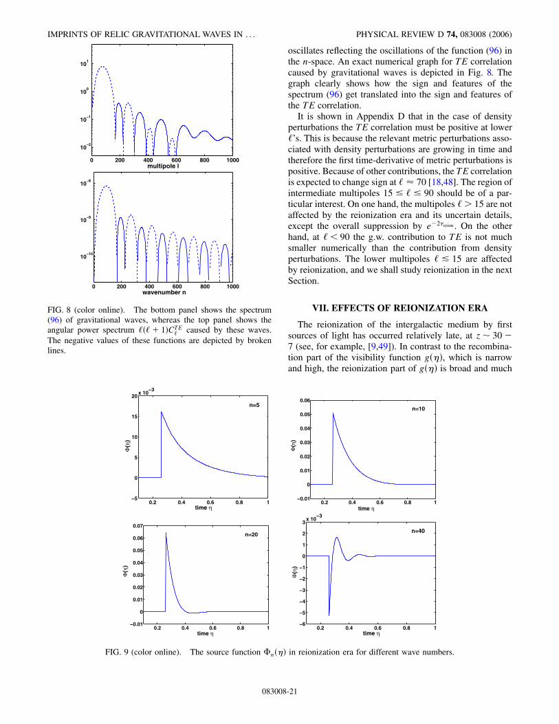
oscillates reflecting the oscillations of the function (96) inthe n-space. An exact numerical graph for TE correlationcaused by gravitational waves is depicted in Fig. 8. Thegraph clearly shows how the sign and features of thespectrum (96) get translated into the sign and features ofthe TE correlation.

It is shown in Appendix D that in the case of densityperturbations the TE correlation must be positive at lower‘’s. This is because the relevant metric perturbations asso-ciated with density perturbations are growing in time andtherefore the first time-derivative of metric perturbations ispositive. Because of other contributions, the TE correlationis expected to change sign at ‘ 70 [18,48]. The region ofintermediate multipoles 15 ‘ 90 should be of a par-ticular interest. On one hand, the multipoles ‘ > 15 are notaffected by the reionization era and its uncertain details,except the overall suppression by e2reion . On the otherhand, at ‘ < 90 the g.w. contribution to TE is not muchsmaller numerically than the contribution from densityperturbations. The lower multipoles ‘ & 15 are affectedby reionization, and we shall study reionization in the nextSection.

VII. EFFECTS OF REIONIZATION ERA

The reionization of the intergalactic medium by firstsources of light has occurred relatively late, at z 307 (see, for example, [9,49]). In contrast to the recombina-tion part of the visibility function g, which is narrowand high, the reionization part of g is broad and much

0 200 400 600 800 1000

10−2

10−1

100

101

multipole l

0 200 400 600 800 1000

10−10

10−9

10−8

wavenumber n

FIG. 8 (color online). The bottom panel shows the spectrum(96) of gravitational waves, whereas the top panel shows theangular power spectrum ‘‘ 1CTE‘ caused by these waves.The negative values of these functions are depicted by brokenlines.

0.2 0.4 0.6 0.8 1−5

0

5

10

15

20x 10

−3

time η

Φ(η

)

n=5

0.2 0.4 0.6 0.8 1−0.01

0

0.01

0.02

0.03

0.04

0.05

0.06

time η

Φ(η

)

n=10

0.2 0.4 0.6 0.8 1−0.01

0

0.01

0.02

0.03

0.04

0.05

0.06

0.07

time η

Φ(η

)

n=20

0.2 0.4 0.6 0.8 1−6

−5

−4

−3

−2

−1

0

1

2

3x 10

−3

time η

Φ(η

)

n=40

FIG. 9 (color online). The source function n in reionization era for different wave numbers.


083008-21

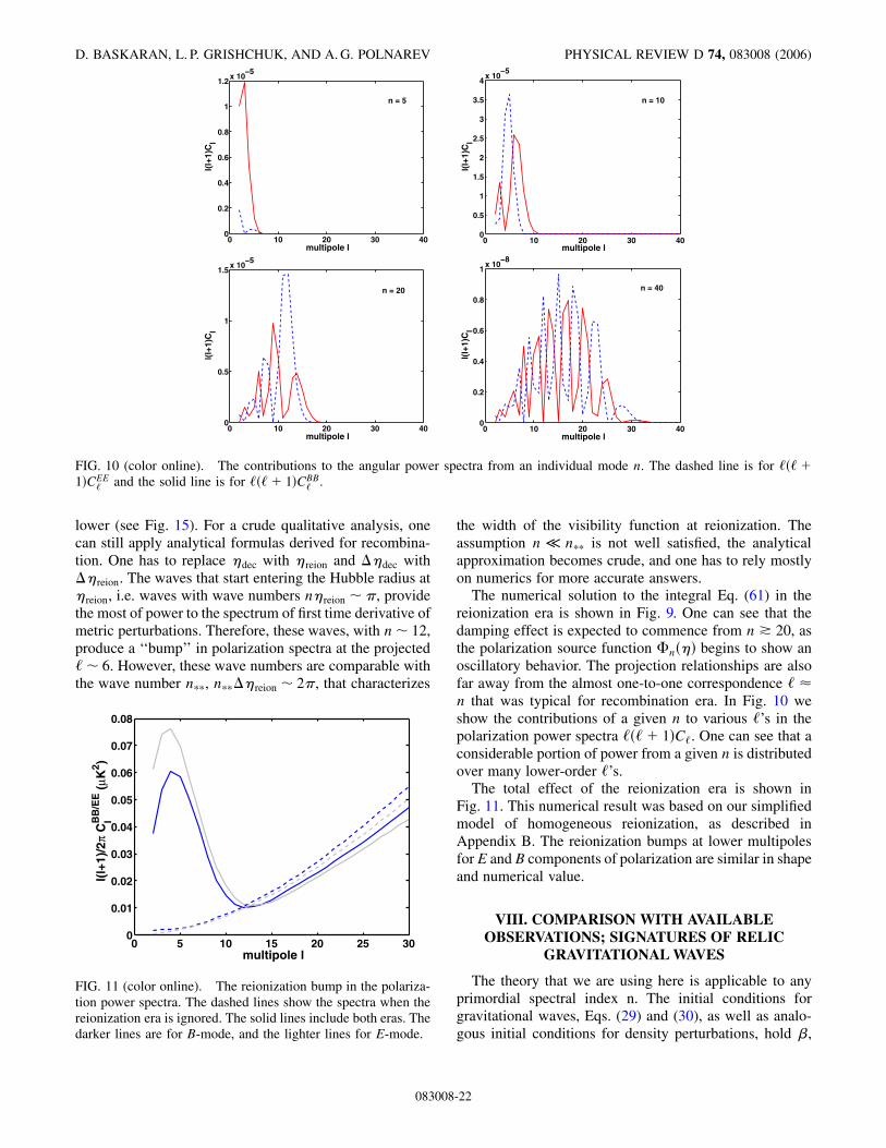
lower (see Fig. 15). For a crude qualitative analysis, onecan still apply analytical formulas derived for recombina-tion. One has to replace dec with reion and dec withreion. The waves that start entering the Hubble radius atreion, i.e. waves with wave numbers nreion , providethe most of power to the spectrum of first time derivative ofmetric perturbations. Therefore, these waves, with n 12,produce a ‘‘bump’’ in polarization spectra at the projected‘ 6. However, these wave numbers are comparable withthe wave number n , n reion 2, that characterizes

the width of the visibility function at reionization. Theassumption n n is not well satisfied, the analyticalapproximation becomes crude, and one has to rely mostlyon numerics for more accurate answers.

The numerical solution to the integral Eq. (61) in thereionization era is shown in Fig. 9. One can see that thedamping effect is expected to commence from n * 20, asthe polarization source function n begins to show anoscillatory behavior. The projection relationships are alsofar away from the almost one-to-one correspondence ‘ n that was typical for recombination era. In Fig. 10 weshow the contributions of a given n to various ‘’s in thepolarization power spectra ‘‘ 1C‘. One can see that aconsiderable portion of power from a given n is distributedover many lower-order ‘’s.

The total effect of the reionization era is shown inFig. 11. This numerical result was based on our simplifiedmodel of homogeneous reionization, as described inAppendix B. The reionization bumps at lower multipolesforE andB components of polarization are similar in shapeand numerical value.

VIII. COMPARISON WITH AVAILABLEOBSERVATIONS; SIGNATURES OF RELIC

GRAVITATIONAL WAVES

The theory that we are using here is applicable to anyprimordial spectral index n. The initial conditions forgravitational waves, Eqs. (29) and (30), as well as analo-gous initial conditions for density perturbations, hold ,

0 5 10 15 20 25 300

0.01

0.02

0.03

0.04

0.05

0.06

0.07

0.08

multipole l

l(l+

1)/2

π C

lBB

/EE (

µK2 )

FIG. 11 (color online). The reionization bump in the polariza-tion power spectra. The dashed lines show the spectra when thereionization era is ignored. The solid lines include both eras. Thedarker lines are for B-mode, and the lighter lines for E-mode.

0 10 20 30 400

0.2

0.4

0.6

0.8

1

1.2x 10

−5

multipole l

l(l+

1)C

l

n = 5

0 10 20 30 400

0.5

1

1.5

2

2.5

3

3.5

4x 10

−5

multipole l

l(l+

1)C

l

n = 10

0 10 20 30 400

0.5

1

1.5x 10

−5

multipole l

l(l+

1)C

l

n = 20

0 10 20 30 400

0.2

0.4

0.6

0.8

1x 10

−8

multipole l

l(l+

1)C

l

n = 40

FIG. 10 (color online). The contributions to the angular power spectra from an individual mode n. The dashed line is for ‘‘1CEE‘ and the solid line is for ‘‘ 1CBB‘ .


083008-22

and hence n, as a free constant parameter. The spectralindex n can be larger, equal, or smaller than 1. However,from the theoretical point of view, the ‘‘red’’ primordialspectra n< 1 (<2) seem to be unacceptable, or atleast questionable. If <2, the mean-square fluctua-tions of gravitational field, Eq. (12), are power-law diver-gent in the limit of very small wave numbers n. One couldargue that the extrapolation of the primordial spectrum tothe ‘‘infrared’’ region of very small n’s is uncertain, and forsome reason the shape of the spectrum bends in the infra-red region making the integral (12) convergent at the lowerlimit. We prefer not to hide behind this possibility. If theshape of the primordial spectrum is allowed to be varied,then practically anything in the CMB data can be explainedby the properly adjusted primordial spectrum. Therefore,our theoretical preference (unless the data will enforce usto change this preference) is a constant primordial spectralindex n> 1 (>2). Obviously, such primordial spectraentail no difficulty in the ‘‘ultraviolet’’ region of very largen’s, because such short-wavelength fluctuations (today’swavelength 3 cm.) did not satisfy the requirements ofsuperadiabatic amplification and simply have not beengenerated.

We now return to the TE correlation. In Fig. 12 we showthe contributions to the TE correlation function from relicgravitational waves (gw) and primordial density perturba-tions (dp). (In order to enhance lowest ‘’s we use thecombination ‘ 1C‘ rather than ‘‘ 1C‘.) For thisillustration, we choose a flat primordial spectrum n 1( 2) and assume equal contributions from (gw) and(dp) to the temperature quadrupole: R 1, where

R CTT‘2gw=CTT‘2dp:

We include the effects of reionization according to themodel with reion 0:09. The (gw) contribution is numeri-cally calculated from the solution to the integral Eq. (61),whereas the (dp) contribution is plotted according to theCMBfast code [18,31]. One can see from the graph that thenegative TE correlation function at lower ‘’s is only pos-sible if there is a significant amount of primordial gravita-tional waves. One can also see from the graph that amisinterpretation of the total TE effect as being causedby density perturbations alone, could lead to a seriousmisestimation of reion.

The TE correlation at lower ‘’s measured by the WMAPmission [9,48] shows clusters of data points, including thenegative ones, that lie systematically below the theoreticalcurve based on density perturbations alone. It is true thatthe data points in the interval 10 & ‘ & 70 are concen-trated near a zero level, the error bars are still large, and themeasured TE correlation can be appreciably different fromthe theoretical statistically averaged TE correlation.However, the recent paper [9], page 26, explicitly empha-sizes the detection of the TE anticorrelation by WMAP:‘‘The detection of the TE anticorrelation near ‘ 30 is afundamental measurement of the physics of the formationof cosmological perturbations. . .’’. As we have alreadystated several times, the TE anticorrelation at lower ‘’s,such as ‘ 30, can only take place (within the frameworkof all other common assumptions) when a significantamount of relic gravitational waves is present.

Our theoretical position, as explained in this and pre-vious papers, is such that we are asking not if relic gravi-tational waves exist, but where they are hiding in thepresently available data. We shall now discuss some mod-els that fit the CMB data and contain significant amounts ofrelic gravitational waves. More accurate observations withWMAP, and especially Planck, should firmly settle on theissue of the sign and value of the TE correlation at lowermultipoles. Hopefully, these observations will establish thepresence of relic gravitational waves beyond reasonabledoubts.

To sharpen the discussion of allowed parameters, wetake the model with n 1:2, reion 0:09 and R 1. Wetake the values mh2 0:03, bh2 0:12, h 0:75, andwe normalize the g.w. contribution to ‘‘1

2 CTT‘ 440 K2 at ‘ 2. In Fig. 13(a) we show our calculationof the TT correlation function in comparison with WMAPdata and the best fit CDM model [8], [18]. (If it comes tothe necessity of explaining ‘‘dark energy’’, natural mod-ifications of general relativity will be superior to unnaturalmodifications of the matter sector [50].) One can see fromthe graph that even this model (which lies, arguably, on asomewhat extreme end) is consistent with the TT data at all‘’s and significantly alleviates the much discussed tensionbetween theory and experiment at ‘ 2. In Fig. 13(b) weshow the TE correlation for exactly the same model. Onecan see that the inclusion of relic gravitational waves

101

102

−0.5

0

0.5

1

multipole l

(l+

1)/2

π C

lTE (

µK2 )

FIG. 12 (color online). The dotted line shows the contributionof density perturbations alone, and the dashed line shows thecontribution of gravitational waves alone. The solid line is thesum of these contributions. It is seen from the graph that theinclusion of g.w. makes the total curve to be always below thed.p. curve.


083008-23

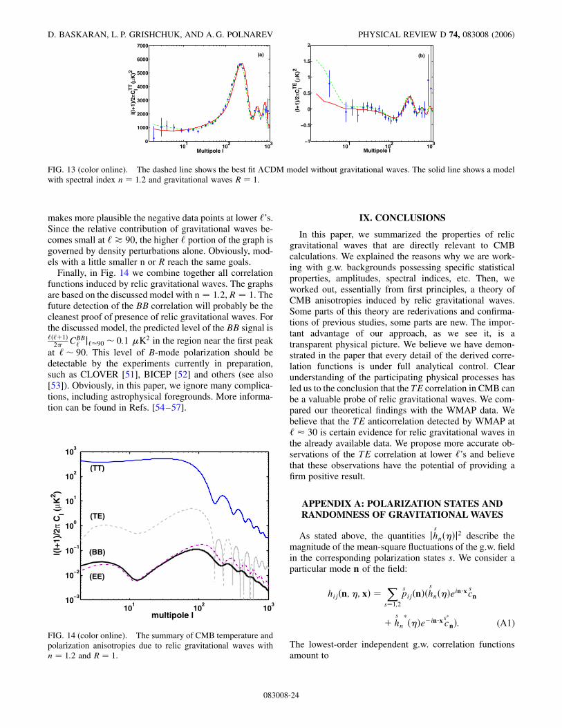
makes more plausible the negative data points at lower ‘’s.Since the relative contribution of gravitational waves be-comes small at ‘ * 90, the higher ‘ portion of the graph isgoverned by density perturbations alone. Obviously, mod-els with a little smaller n or R reach the same goals.

Finally, in Fig. 14 we combine together all correlationfunctions induced by relic gravitational waves. The graphsare based on the discussed model with n 1:2, R 1. Thefuture detection of the BB correlation will probably be thecleanest proof of presence of relic gravitational waves. Forthe discussed model, the predicted level of the BB signal is‘‘1

2 CBB‘ j‘90 0:1 K2 in the region near the first peakat ‘ 90. This level of B-mode polarization should bedetectable by the experiments currently in preparation,such as CLOVER [51], BICEP [52] and others (see also[53]). Obviously, in this paper, we ignore many complica-tions, including astrophysical foregrounds. More informa-tion can be found in Refs. [54–57].

IX. CONCLUSIONS

In this paper, we summarized the properties of relicgravitational waves that are directly relevant to CMBcalculations. We explained the reasons why we are work-ing with g.w. backgrounds possessing specific statisticalproperties, amplitudes, spectral indices, etc. Then, weworked out, essentially from first principles, a theory ofCMB anisotropies induced by relic gravitational waves.Some parts of this theory are rederivations and confirma-tions of previous studies, some parts are new. The impor-tant advantage of our approach, as we see it, is atransparent physical picture. We believe we have demon-strated in the paper that every detail of the derived corre-lation functions is under full analytical control. Clearunderstanding of the participating physical processes hasled us to the conclusion that the TE correlation in CMB canbe a valuable probe of relic gravitational waves. We com-pared our theoretical findings with the WMAP data. Webelieve that the TE anticorrelation detected by WMAP at‘ 30 is certain evidence for relic gravitational waves inthe already available data. We propose more accurate ob-servations of the TE correlation at lower ‘’s and believethat these observations have the potential of providing afirm positive result.

APPENDIX A: POLARIZATION STATES ANDRANDOMNESS OF GRAVITATIONAL WAVES

As stated above, the quantities jhs

nj2 describe the

magnitude of the mean-square fluctuations of the g.w. fieldin the corresponding polarization states s. We consider aparticular mode n of the field:

hijn; ;x Xs1;2

psijnh

s

neinxcs

n

hs

n

einxc

s

n: (A1)

The lowest-order independent g.w. correlation functionsamount to

101

102

103

10−3

10−2

10−1

100

101

102

103

multipole l

l(l+

1)/2

π C

l (µK

2 )

(TT)

(TE)

(BB)

(EE)

FIG. 14 (color online). The summary of CMB temperature andpolarization anisotropies due to relic gravitational waves withn 1:2 and R 1.

101

102

1030

1000

2000

3000

4000

5000

6000

7000

Multipole l

l(l+

1)/2

πClT

T (µK

)2

(a)

101

102

103−1

−0.5

0

0.5

1

1.5

2

Multipole l

(l+

1)/2

πClT

E (µK

)2

(b)

FIG. 13 (color online). The dashed line shows the best fit CDM model without gravitational waves. The solid line shows a modelwith spectral index n 1:2 and gravitational waves R 1.


083008-24

hhijn; ;xps ijnhkln0; ;x0p

s0 kln0i

8jhs

nj2ss03n n0: (A2)

The action of the random g.w. field (A1) on free particlesleads to their relative oscillatory motion. We refer thismotion to a local inertial frame. Let a ring of free particlesto lie in the l;m-plane; the ring encircles the axis n.Then, the mean-square amplitude of oscillations in the ’’

polarization state is determined by jh1

nj2, whereas the

mean-square amplitude of oscillations in the ’’ polariza-

tion state is determined by jh2

nj2. In general, the random

gravitational-wave field can be such that the oscillation

amplitudes jh1

nj2 and jh

2

nj2 are different. But if jh

1

nj2

jh2

nj2, then the (averaged) observed picture of oscillations

is not symmetric with respect to rotations around n.Formally, the correlation functions of the field with

jh1

nj2 jh

2

nj2 do not have symmetry with respect to the

change of polarization basis. Indeed, the transition to theprimed basis according to Eq. (7) brings the gravitational-wave mode (A1) to the form

hijn; ;x Xs1;2

ps 0ijnb

s

neinx b

s

neinx;

where

b1

n cos2 h1

nc1

n sin2 h2

nc2

n;

b2

n sin2 h1

nc1

n cos2 hn2

nc2

n:

Taking into account the relationships (16), we can nowderive the correlation functions for the new polarizationcomponents:

hb1

nb1

n0 i jh1

nj2cos22 jh

2

nj2sin22 3n n0;

hb2

nb2

n0 i jh1

nj2sin22 jh

2

nj2cos22 3n n0;

hb1

nb2

n0 i jh1

nj2 jh

2

nj2 sin2 cos2 3n n0:

(A3)

It is seen from (A3) that, in general, the -dependencesurvives, and the assumption of statistical independence ofpolarization components in one basis is not equivalent tothis assumption in another basis. However, one recoversthe original correlation functions (A2) from (A3) if theconditions (18) are fulfilled.

Similar properties hold true for circular polarizations. Ag.w. mode hijn; ;x expanded over circular polarizationstates is given by

hijn; ;x hijn; ;x h ijn; ;x;

where

h ijn; ;x XsL;R

psijnh

s

neinxc

sn: (A4)

We assume that the complex random coefficients cs

n s L;R, satisfy the statistical conditions (16).

The relevant independent correlation functions are cal-culated to be

h hijn; ;xps ij n h kln

0; ;x0ps0 kln0i

4jhs

nj2ss03n n0; s L;R: (A5)

If the observer views the motion of test particles from then direction, i.e. against the direction of the incoming

gravitational wave, the function jhR

nj2 is responsible forthe mean-square amplitude of the right-handed (clockwise)

rotations of individual particles. The function jhL

nj2 isresponsible for the left-handed (counter-clockwise) rota-tions. (For more details about the motion of free particles inthe field of gravitational waves, see [41].)

Expansion (A4) preserves its form under transforma-

tions (21), if one makes the replacements: hL0

n Lh

nei2 ,

hR0

n hR

nei2 . Therefore, the correlation functions (A5) do

not change, regardless the value of the amplitudes jhs

nj2

s L;R. On the other hand, discrete transformations

(22) generate the replacements: hL0

n hR

n, hR0

n hL

n.Therefore, the sense of correlation functions (A5) changesfrom L to R and vice versa. The symmetry between left andright is violated, unless the conditions (23) are fulfilled.

APPENDIX B: ASTROPHYSICAL PREREQUISITES

1. Ionization history

The ionization history of the Universe enters our equa-tions through the density of free electrons Ne, i.e.electrons available for Thompson scattering. Specifically,we operate with the quantity q:

q TaNe: (B1)

The optical depth between some instant of time 0 and alater instant is defined by the integral

;0 Z

0d00q00:

The optical depth from some to the present time R isdenoted and is given by

R; Z R

d0q0:

It follows from the above definitions that ;0 0 .


083008-25

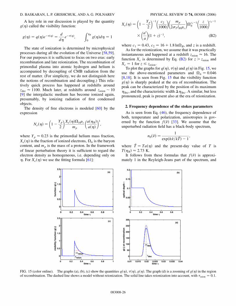
A key role in our discussion is played by the quantityg called the visibility function:

g qe dd

e;Z R

0gd 1

The state of ionization is determined by microphysicalprocesses during all the evolution of the Universe [58,59].For our purposes it is sufficient to focus on two eras: earlyrecombination and late reionization. The recombination ofprimordial plasma into atomic hydrogen and helium isaccompanied by decoupling of CMB radiation from therest of matter. (For simplicity, we do not distinguish herethe notions of recombination and decoupling.) This rela-tively quick process has happened at redshifts aroundzdec 1100. Much later, at redshifts around zreion 10[9] the intergalactic medium has become ionized again,presumably, by ionizing radiation of first condensedobjects.

The density of free electrons is modeled [60] by theexpression

Ne

1Yp2

Xebc

mp

aRa

3;

where Yp 0:23 is the primordial helium mass fraction,Xe is the fraction of ionized electrons, b is the baryoncontent, and mp is the mass of a proton. In the frameworkof linear perturbation theory it is sufficient to regard theelectron density as homogeneous, i.e. depending only on. For Xe we use the fitting formula [61]:

Xe

1Yp2

1c2

1000

mp

2TlHc

c11b

z

1000

c21

a0

a

1 z1; (B2)

where c1 0:43, c2 16 1:8 lnB, and z is a redshift.As for the reionization, we assume that it was practically

instantaneous and happened at a redshift zreion 16. Thefunction Xe is determined by Eq. (B2) for z > zreion andXe 1 for z zreion.

To plot the graphs for q, and g in Fig. 15, weuse the above-mentioned parameters and b 0:046[8,18]. It is seen from Fig. 15 that the visibility functiong is sharply peaked at the era of recombination. Thepeak can be characterized by the position of its maximumdec, and the characteristic width dec. A similar, but lesspronounced, peak is present also at the era of reionization.

2. Frequency dependence of the stokes parameters

As is seen from Eq. (46), the frequency dependence ofboth, temperature and polarization, anisotropies is gov-erned by the function f~ [33]. We assume that theunperturbed radiation field has a black-body spectrum,

n0~ 1

exph~=k~T 1;

where ~T Ta and the present-day value of T isTR 2:73 K.

It follows from these formulas that f~ is approxi-mately 1 in the Reyleigh-Jeans part of the spectrum, and

0 0.2 0.4 0.6 0.8 1

0

0.5

1

1.5

2

2.5

time η

fu

nct

ion

q(η

)

(a)

0 0.2 0.4 0.6 0.8 1

0

0.05

0.1

0.15

0.2

time η

op

tica

l dep

th τ

(b)

0 0.2 0.4 0.6 0.8 1

0

0.5

1

1.5

2

2.5

time η

vis

ibili

ty f

un

ctio

n g

(η)

(c)

ηreion

∆ηreion

0.01 0.015 0.02 0.025 0.03 0.035 0.04

0

50

100

150

200

250

300

time η

g(η

) at

rec

om

bin

atio

n

∆ηdec

ηdec

(d)

FIG. 15 (color online). The graphs (a), (b), (c) show the quantities q, , g. The graph (d) is a zooming of g in the regionof recombination. The dashed line shows a model without reionization. The solid line takes reionization into account, with reion 0:1.


083008-26

f~ varies as h~=k~T in the Wein part. In practice, we areusually interested in the total intensity, i.e. Stokes parame-ters integrated over all photon frequencies. This integrationproduces the factor :

Zd~h~3

c2 n0~f~ 4I0; (B3)

where I0 Rd~ h~3

c2 n0~ is the total intensity of the un-perturbed radiation field. The factor often appears in themain text of the paper.

APPENDIX C: TWO ESSENTIAL VARIABLES FORTEMPERATURE AND POLARIZATION

It is seen from Eq. (48) that the frequency dependence ofn1 is determined by the factor f~n0~. Therefore, wecan single out this factor and write

n 1; ~;; 1

2f~n0~n1;;:

The equation that follows from (48) and (49) reads

@@ q in

n1;; 12e2i dhn

du

q4

Z 1

1

Z 2

0d0d0P;;0; 0n1;0; 0:

(C1)

The quantity n1;; as a function of can be expanded in a series

n 1;; X1

m1

n1m ;eim: (C2)

The explicit structure of the Chandrasekhar matrix P;;0; 0 is given by the expression [29] (equation (220) onp. 42):

P;;0; 0 QP0 121=21021=2P1 P2;

where matrices Q, P0;0, P1;;0; 0, P2;;0; 0 read

Q

1 0 0

0 1 0

0 0 2

0BB@1CCA;

P0 3

4

212102 202 2 0

02 1 0

0 0 0

0BB@

1CCA;

P1 3

4

40 cos0 0 2 sin0

0 0 0

20 sin0 0 cos0

0BB@

1CCA;

P2 3

4

202 cos20 2 cos20 20 sin20

02 cos20 cos20 0 sin20

02 sin20 sin20 0 cos20

0BB@1CCA:

The structure of the Chandrasekhar matrixP;;0; 0 is such that it does not mix them-dependence, that is,

1

4

Z 1

1

Z 2

0d0d0P;;0; 0n1m ;0eim

0

eim:

Moreover, this integral vanishes for all jmj> 2. Thismeans that Eq. (C1) is a homogeneous differential equation

for all n1m with m 2. Assuming zero initial conditionsat some initial , we obtain n1m 0 for all m 2.Hence, we are left with three functions of ;:

n 1;; n1;e2i: (C3)

We are now able to show that only two out of the threefunctions n1; are independent. Indeed, using (C3) inEq. (C1) we arrive at a system of three linear equations forthe components of n1;:


083008-27

@@ q in

n1;n2;n3;

0@ 1A

12dhnd

110

0@ 1A 3

8q

2

12i

0B@1CAI; (C4)

where I is the remaining integral that was left overfrom the last term in Eq. (C1):

I 1

2

Z 1

1d002n1;

0 n2;0

i0n3;0: (C5)

Despite the complicated appearance, only two of thethree Eqs. (C4) are really coupled. Indeed, making linearcombinations of Eqs. (C4) it is easy to show that thecombination 2in1 n2 1

2n3 satisfies a homo-geneous differential equation. Assuming zero initial con-ditions, we derive

2in1 n2 12n3 0:

As two independent and essential variables we choose

; n1; n2;

12;

; n1; n2;

12

n3;2i

:

In terms of and equations of radiative transfer reduceto Eq. (51) and (52), and the definition (C5) for I takesthe form of Eq. (53).

Although we have considered a gravitational-wave per-turbation, the existence of only two essential variables is ageneral statement and it applies to density and rotationalperturbations as well. In general, the perturbed radiativetransfer equation contains an arbitrary function f;;in front of u, rather than a specific combination12e2idhn=d quoted in Eq. (C1). Functionf;; can be expanded in a series similar to Eq. (C2):

f;; X1

m1

fm;eim:

Since the scattering integral (second term in the r.h.s ofEq. (C1)) vanishes for all jmj> 2, the functions n1m ;are fully determined by fm; (jmj> 2) and describethe temperature variations only. To discuss polarization, wehave to consider three remaining cases m 0, 1, 2.

The explicit identification of the two essential variables; and ; for the case m 2 has been given

above. Specifically for gravitational waves, f2

12dhL

n=d, f2 12dhR

n=d.The identification of the two essential variables for the

case m 0 proceeds in a similar manner. Having calcu-

lated the scattering integral for m 0 one can show thatthe equation, analogous to Eq. (C4), will now read

@@ q in

n1;n2;n3;

0@ 1A

f0; qI10

110

0@ 1A 3

8q

32 2

10

0B@1CAJ ;

where

I10 1

4

Z 1

1d0n1;0 n2;0;

J 1

3

Z 1

1d0302 2n1;

0 n2;0:

Obviously, n3 satisfies a homogeneous equation and can beput to zero. Specifically for density perturbations (seeAppendix D), function f0; consists of terms repre-senting gravitational-field perturbations and the Dopplerterm arising due to the baryon velocity:

f0; 1

2

dhd2 dhl

d iqvb

:

We have checked that in the case m 1 the problemalso reduces to only two essential variables. The combina-tion n1 n2 in3 vanishes at the zero initial data.

APPENDIX D: TEMPERATURE ANDPOLARIZATION ANISOTROPIES CAUSED BY

DENSITY PERTURBATIONS

To discover relic gravitational waves in the CMB datawe have to distinguish their effects from the effects ofdensity perturbations. The theory of temperature and po-larization anisotropies caused by primordial density per-turbations is very much similar to the theory of relicgravitational waves. We start from the metric Fourierexpansion (10) with the polarization tensors (9). Havingderived and solved integral equations of radiative transferin the presence of density perturbations, we arrive at ourfinal goal of distinguishing the TE cross-correlations.

1. Radiative transfer equations

The equations of radiative transfer in the presence of asingle mode n of density perturbations are similar toEq. (48) and read


083008-28

@@ q ieini

n1n ; ~; ei

f~n0~

2

eiejp

sijn

dhs

nd

qeivi

u

q4

Zd0Pei; e0jn1n ; ~; e0j; (D1)

where the extra term eivi takes care of the movement ofscattering electrons with respect to the chosen synchronouscoordinate system [62–64].

For technical reasons, it is convenient to work with the‘‘scalar’’ h and ‘‘longitudinal’’ hl polarization mode

functions, instead of the original hs

n [65]. The relation-ship between them is

h1n

3

2

sh hl; h

2

n

1

3

shl;

where the wave number index n on h and hl is

implicit. Both polarization components of metric perturba-tions participate in Eq. (D1). In the frame associated withthe density wave, i.e. for n=n 0; 0; 1, the structureseiejp

sij (see Eq. (9)) and eivi ivb depend on

cos, but not on the azimuthal angle .By argumentation similar to that in Appendix C, one can

show that a solution (not vanishing on zero initial data) toEq. (D1) must have the form

n1n ; ~; f~n0~

2

264n;1

1

0

0BB@1CCA

n;

1

1

0

0BB@

1CCA375: (D2)

Substituting Eq. (D2) into Eq. (D1) we arrive at a system ofcoupled equations for and

@@ q in

n;

1

2

dhd2 dhl

d

q

I1 ivb

1

2P2I2

; (D3a)

@@ q in

n;

1

2q1 P2I2; (D3b)

where

I1 1

2

Z 1

1dn;; (D4a)

I2 1

2

Z 1

1d1 P2n; P2n; (D4b)

The quantity I1 is the monopole component of the perturbed radiation field, whereas I2 is the quadrupole (‘ 2)component, responsible for the generation of polarization.

To make contact with previous work we note that the variables and are closely related to the variables T and Pfrom Ref. [31]. Assuming a black body unperturbed radiation field, we have T , P . We also note that themode functions h and hl are related to the mode functions h and used in [31,64] by h 2, hl h 6. Keepingin mind the difference in notations, one can verify that Eqs. (D3a) and (D3b) are equivalent to equations (11) in Ref. [31].

2. Integral equations and their solutions

A formal solution to Eqs. (D3a) and (D3b) can be written as

n; Z

0d0e;

0in0

1

2

dhd2 dhl

d

q

I1 ivb

1

2P2I2

; (D5a)

n; 1

21 P2

Z

0d0e;

0in0I2: (D5b)

Proceeding in a manner similar to that in Sec. IV, we substitute (D4a) and (D5b) into (D4a) and (D4b). After certainrearrangements we arrive at two coupled integral equations for I1 and I2:


083008-29

I1 Z

0d0q0e;

0

I10j0x

1

2I20j2x

Z

0d0e;

0

1

2

dhd0

j0x dhld0

d2j0

dx2

q0vb

0j1x; (D6a)

I2 Z

0d0q0e;

0

I1

0j2x I20

18

x2 1

2

j2x

3

2xj1x

Z

0d0e;

0

1

2

dhd0

j2x dhld0

j2x 3

d2j0

dx2

q0vb0

dj2

dx

; (D6b)

where the argument of spherical Bessel functions j‘x isx n 0.

Eqs. (D6a) and (D6b) together with the continuity equa-tions for matter perturbations and Einstein equations formetric perturbations (see for example [64,65]), form aclosed system of coupled integro-differential equations.In previous treatments [31,63,64], the radiative transferequations were presented as an infinite series of coupledordinary differential equations.

Similarly to what was done in Sec. IV B, we can analyzeEqs. (D6a) and (D6b) in terms of expansions in powers ofn,

I 1 X1k0

I k1 n2k; I2

X1k0

I k2 n2k: (D7)

The kernels of Eqs. (D6a) and (D6b) are expanded inpowers of x. In the long-wavelength approximation, i.e.for x 1, we can limit ourselves by first nonvanishingterms. The zero-order approximation brings us to the equa-tions

I 01 Z

0d0q0e;

0I 01 0

Z

0d0e;

0

1

2

dhd0

1

3

dhld0

1

3q0vb

0x;

I 02 7

10

Z

0d0q0e;

0I 02 0

1

15

Z

0d0e;

0

dhld0 2q0vb

0x:

The solution to these equations is given by

I 01 Z

0d0

1

2

dhd0

1

3

dhld0

1

3nZ 0

0d00q00e

0;00vb00

; (D8a)

I 02 1

15

Z

0d0e3=10;0

dhld0 2n

Z 0

0d00q00e

0;00vb00:

(D8b)

3. Multipole coefficients

We are mostly interested in the present-day values of and and, hence, we put R in (D5a) and (D5b).Irrespective of approximation in which the functionsI1, I2 are known, the multipole coefficients forthe radiation field can be found in a way similar to thatin Sec. V:

aT‘mn i‘

42‘ 1

pm0aT‘ n;

aE‘mn i‘

42‘ 1

pm0aE‘ n; aB‘mn 0;

where aT‘ n, aE‘ n are given by

aT‘ n Z R

0d

e

1

2

dhd

1

2

dhld

d2

d2

gI1 vb

dd

3

4I2

1

d2

d2

j‘;

(D9a)

aE‘ n 3

4

‘ 2!

‘ 2!

1=2 Z R

0dgI2

j‘

2 ; (D9b)

and nR . As expected, in the case of densityperturbations all a‘m 0 for m 0 and aB‘mn 0,[31,32,66,67]. The formal reason for this is that all quan-tities in (D2) do not depend on (A more detailed ex-position can be found in [31,32]).

Let us start from the temperature multipoles. For illus-tration, we consider an instantaneous recombination. Wereplace e with the step function, g with the-function, and we neglect the I2 term. Then, we get

aT‘ n

I1 vbdd

j‘

dec

1

2

Z R

dec

ddhddhld

d2

d2

j‘:

This expression can be further simplified by taking theremaining integral by parts. After some rearrangementswe arrive at the final expression


083008-30

aT‘ n

1

2n2

d2hld2 ‘0

1

6ndhld

‘1

R

1

2n2

d2hld2 I1

1

2ndhld vb

dd

j‘dec

1

2

Z R

dec

ddhd

1

n2

d3hld3

j‘: (D10)

For the growing mode of density perturbations in thematter-dominated era, the integrand of the remaining in-tegral vanishes. If, in addition, the intrinsic temperatureperturbation I1 and the plasma velocity vb are zero at dec, we recover from Eq. (D10) the four terms of the fullSachs-Wolfe formula (43) in Ref. [68]. We would like tonote in passing that the origin of the often used, includingthis paper, combination ‘‘ 1C‘ is in fact a historicalaccident, when a wrong motivation leads to a convenientnotation. This combination arises in the essentially incor-rect formula ‘‘ 1C‘ const that can be derived afterthe unjustified neglect of three out of four terms in theoriginal Sachs-Wolfe formula (43) in Ref. [68]. This clari-fication is important not only by itself, but also for correctphysical interpretation of reasons for the rise toward the‘‘first peak’’ at ‘ 220 of the actually observed function‘‘ 1C‘. For more details, see [69].

We now turn to polarization anisotropies. We use thezero-order approximation (D8b) in (D9b),

aE‘ 1

20

‘ 2!

‘ 2!

1=2 Z R

0dqe7=10 j‘

2

Z

0d0e3=100

dhld0

2nZ 0

0d00q00e

0;00vb00:

As g is a narrow function, the integrand is localizednear dec. By the same argumentation that was usedin Sec. VI B, the above expression can be reduced toquantities evaluated at dec,

aE‘ n1

20

‘2!

‘2!

1=2j‘2

dhld

2nvb ~dec

;

(D11)

where the factors and ~ are of the order of the width ofg in the recombination era. Explicitly, they are given by

Z R

0dg

Z

0d0e3=10;0;

~ Z R

0dg

Z

0d0e3=10;0

Z 0

0d00q00e

0;00:

The angular power spectra in the case of density pertur-bations are described by formulas analogous to (86). By thesteps similar to those in Sec. V C it can be shown that thepower spectra are given by

CXX0

‘ C2

ZndnaX‘ na

X0‘ n; (D12)

where C for density perturbations is C 24p

lPl.

4. Temperature-polarization correlations

We focus on the TE correlation at the relatively smallmultipoles, ‘ & 70. The dominant contribution to thesemultipoles comes from density perturbations that did notenter the Hubble radius at recombination, n & 70. It issufficient to consider the early time evolution of theseperturbations in the matter-dominated era.

Restricting our analysis to the growing mode, we writefor the metric and matter perturbations (see, for example,[65]):

h Bn const; hl Bnn2;

I 01 TT

2

3Bnn

2; vb 2

9Bnn

3:

Substituting this solution into (D10) and (D11) and takinginto account only the lowest-order terms in n (the long-wavelength approximation) we arrive at

aT‘ Bnj‘jdec; (D13a)

aE‘ 1

10n2Bndec

‘ 2!

‘ 2!

1=2j‘

2

rec

:

(D13b)

Finally, from Eq. (D12) we obtain for the TE correlation:

CTE‘ C2

dec

10

‘ 2!

‘ 2!

1=2 Z

dnn3B2n

j‘

2dec

:

(D14)

All terms in the above expression are strictly positive.Therefore, the TE correlation caused by density perturba-tions, in contrast to the case of gravitational waves, must bepositive at lower multipoles ‘ & 50 where our approxima-tions are still valid. As mentioned before, this differencebetween gravitational waves and density perturbationsboils down to the difference in the sign of first time-derivative of the associated metric perturbations.


083008-31

[1] J. Bock et al., astro-ph/0604101.[2] L. P. Grishchuk, Zh. Eksp. Teor. Fiz. 67, 825 (1974) [Sov.

Phys. JETP 40, 409 (1975)]; Ann. N.Y. Acad. Sci. 302,439 (1977); Pis’ma Zh. Eksp. Teor. Fiz. 23, 326 (1976)[JETP Lett. 23, 293 (1976)].

[3] Ya. B. Zel’dovich and A. A. Starobinsky, Zh. Eksp. Teor.Fiz. 61, 2161 (1971) [Sov. Phys. JETP 34, 1159 (1972)].

[4] L. P. Grishchuk and A. G. Polnarev, in: General Relativityand Gravitation, 100 Years After the Birth of A. Einstein,edited by A. Held (Plenum Press, NY, 1980), Vol. 2,p. 393.

[5] L. P. Grishchuk, Usp. Fiz. Nauk 175, 1289 (2005) [Phys.Usp. 48, 1235 (2005)].

[6] V. N. Lukash, Usp. Fiz. Nauk 176, 113 (2006) [Phys. Usp.49 (2006)].

[7] H. V. Peiris et al., Astrophys. J. Suppl. Ser. 148, 213(2003).

[8] D. N. Spergel et al., astro-ph/0603449.[9] L. Page et al., astro-ph/0603450.

[10] Planck Collaboration, astro-ph/0604069.[11] S. Bose and L. P. Grishchuk, Phys. Rev. D 66, 043529

(2002).[12] E. Newman and R. Penrose, J. Math. Phys. (N.Y.) 7, 863

(1966).[13] J. N. Goldberg et al., J. Math. Phys. (N.Y.) 8, 2155 (1967).[14] K. S. Thorne, Rev. Mod. Phys. 52, 299 (1980).[15] Y. Watanabe and E. Komatsu, Phys. Rev. D 73, 123515

(2006).[16] L. P. Grishchuk and M. Solokhin, Phys. Rev. D 43, 2566

(1991).[17] L. P. Grishchuk, LNP Vol. 562: Gyros, Clocks,

Interferometers . . ., Testing Relativistic Gravity in Space167 (2001).

[18] Legacy Archive for Microwave Background DataAnalysis (LAMBDA), http://lambda.gsfc.nasa.gov.

[19] G. Hinshaw et al., astro-ph/0603451.[20] L. P. Grishchuk, Usp. Fiz. Nauk 156, 297 (1988) [Sov.

Phys. Usp. 31, 940 (1988)].[21] B. Allen and J. D. Romano, Phys. Rev. D 59, 102001

(1999).[22] V. Corbin and N. J. Cornish, Classical Quantum Gravity

23, 2435 (2006).[23] L. A. Boyle and P. J. Steinhardt, astro-ph/0512014.[24] Asantha Cooray, Mod. Phys. Lett. A 20, 2503 (2005).[25] T. L. Smith, M. Kamionkowski, and A. Cooray, Phys. Rev.

D 73, 023504 (2006).[26] T. Smith, H. Peiris, and A. Cooray, Phys. Rev. D 73,

123503 (2006).[27] S. Chongchitnan and G. Efstathiou, astro-ph/0603118.[28] V. Mandic and A. Buonanno, Phys. Rev. D 73, 063008

(2006).[29] S. Chandrasekhar, Radiative Transfer (Dover Publications

Inc., New York, 1960).[30] L. D. Landau and E. M. Lifshitz, The Classical Theory of

Fields (Pergamon Press, Oxford, 1975), 4th rev. engl. ed..[31] M. Zaldarriaga and U. Seljak, Phys. Rev. D 55, 1830

(1997).[32] M. Kamionkowski, A. Kosowsky, and A. Stebbins, Phys.

Rev. D 55, 7368 (1997).

[33] M. M. Basko and A. G. Polnarev, Sov. Astron. 24, 268(1980).

[34] A. G. Polnarev, Sov. Astron. 29, 607 (1985).[35] R. W. Lindquist, Ann. Phys. (N.Y.) 37, 487 (1966).[36] N. Caderni et al., Phys. Rev. D 17, 1901 (1978).[37] P. Naselsky, D. Novikov, and I. Novikov, Adv. Space Res.

31, 417 (2003).[38] R. Crittenden et al., Phys. Rev. Lett. 71, 324 (1993).[39] U. Seljak and M. Zaldarriaga, Phys. Rev. Lett. 78, 2054

(1997).[40] R. A. Frewin, A. G. Polnarev, and P. Coles, Mon. Not. R.

Astron. Soc. 266, L21 (1994).[41] D. Baskaran and L. P. Grishchuk, Classical Quantum

Gravity 21, 4041 (2004).[42] A. N. Varshalovich, D. A. Moskalev, and V. K.

Khersonskii, Quantum Theory of Angular Momentum(World Scientific, Singapore, 1988).

[43] L. P. Grishchuk and J. Martin, Phys. Rev. D 56, 1924(1997).

[44] A. Lue, L. Wang, and M. Kamionkowski, Phys. Rev. Lett.83, 1506 (1999).

[45] B. Allen and S. Koranda, Phys. Rev. D 50, 3713 (1994).[46] J. R. Pritchard and M. Kamionkowski, Ann. Phys. (N.Y.)

318, 2 (2005);[47] W. Zhao and Y. Zhang, astro-ph/0508345.[48] A. Kogut et al., Astrophys. J. Suppl. Ser. 148, 161 (2003).[49] B. Keating and N. Miller, New Astron. Rev. 50, 184

(2006).[50] S. V. Babak and L. P. Grishchuk, Int. J. Mod. Phys. D 12,

1905 (2003).[51] B. Maffei et al., astro-ph/0407148.[52] B. G. Keating et al., in Proceedings of the SPIE, edited by

S. Fineschi (SPIE Press, 2003), Vol. 4843, p. 284.[53] B. Keating, A. G. Polnarev, N. Miller, and D. Baskaran,

Int. J. Mod. Phys. A 21, 2459 (2006).[54] B. Keating et al., Astrophys. J. 495, 580 (1998).[55] M. V. Sazhin, G. Sironi, and O. S. Khovanskaya, New

Astron. Rev. 9, 83 (2004).[56] P. D. Naselsky, I. D. Novikov, and L.-Y. Chiang,

Astrophys. J. 642, 617 (2006).[57] A. Lewis and A. Challinor, Phys. Rep. 429, 1 (2006).[58] P. D. Naselskii and A. G. Polnarev, Astrofizika 26, 543

(1987) [Astrophysics (Engl. Transl.) 26, 327 (1987)].[59] A. G. Doroshkevich, I. P. Naselsky, P. D. Naselsky, and

I. D. Novikov, Astrophys. J. 586, 709 (2003).[60] P. J. E. Peebles, Principles of Physical Cosmology

(Princeton University Press, Princeton, 1993).[61] W. Hu and N. Sugiyama, Astrophys. J. 444, 489 (1995).[62] N. Kaiser, Mon. Not. R. Astron. Soc. 202, 1169 (1983).[63] J. R. Bond and G. Efstathiou, Astrophys. J. Lett. 285, L45

(1984).[64] C.-P. Ma and E. Bertschinger, Astrophys. J. 455, 7 (1995).[65] L. P. Grishchuk, Phys. Rev. D 50, 7154 (1994).[66] U. Seljak, Astrophys. J. 482, 6 (1997).[67] W. Hu and M. White, New Astron. Rev. 2, 323 (1997).[68] R. K. Sachs and A. M. Wolfe, Astrophys. J. 147, 73

(1967).[69] A. Dimitropoulos and L. P. Grishchuk, Int. J. Mod. Phys.

D 11, 259 (2002).


083008-32

Documents

Imprints of relic gravitational waves in cosmic microwave