Important sources for Numpy and Scipy Documentationhomes.ieu.edu.tr/skondakci/courses/CE476/frequency spectrum with scipy.pdf · Transform (FFT) is an efficient method for calculating

Important sources for Numpy and Scipy Documentation

http://wiki.scipy.org/Cookbook

http://docs.scipy.org/doc/

http://docs.scipy.org/doc/scipy/reference/tutorial/

How to plot the frequency spectrum with scipy

Spectrum analysis is the process of determining the frequency domain representation of a time domain signal and most commonly employs the Fourier transform. The Discrete Fourier Transform (DFT) is used to determine the frequency content of signals and the Fast Fourier Transform (FFT) is an efficient method for calculating the DFT. Scipy implements FFT and in this post we will see a simple example of spectrum analysis: from numpy import sin, linspace, pi from pylab import plot, show, title, xlabel, ylabel , subplot from scipy import fft, arange def plotSpectrum(y,Fs): """ Plots a Single-Sided Amplitude Spectrum of y(t) """ n = len(y) # length of the signal k = arange(n) T = n/Fs frq = k/T # two sides frequency range frq = frq[range(n/2)] # one side frequency range Y = fft(y)/n # fft computing and normalization Y = Y[range(n/2)] plot(frq,abs(Y),'r') # plotting the spectrum xlabel('Freq (Hz)') ylabel('|Y(freq)|') Fs = 150.0; # sampling rate Ts = 1.0/Fs; # sampling interval t = arange(0,1,Ts) # time vector ff = 5; # frequency of the signal y = sin(2*pi*ff*t) subplot(2,1,1) plot(t,y) xlabel('Time') ylabel('Amplitude') subplot(2,1,2) plotSpectrum(y,Fs) show()

The program shows the following figure, on top we have a plot of the signal and on the bottom the frequency spectrum.

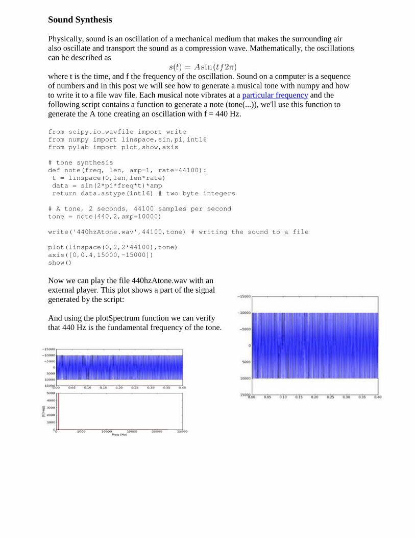
Sound Synthesis

Physically, sound is an oscillation of a mechanical medium that makes the surrounding air also oscillate and transport the sound as a compression wave. Mathematically, the oscillations can be described as

where t is the time, and f the frequency of the oscillation. Sound on a computer is a sequence of numbers and in this post we will see how to generate a musical tone with numpy and how to write it to a file wav file. Each musical note vibrates at a particular frequency and the following script contains a function to generate a note (tone(...)), we'll use this function to generate the A tone creating an oscillation with f = 440 Hz. from scipy.io.wavfile import write from numpy import linspace,sin,pi,int16 from pylab import plot,show,axis # tone synthesis def note(freq, len, amp=1, rate=44100): t = linspace(0,len,len*rate) data = sin(2*pi*freq*t)*amp return data.astype(int16) # two byte integers # A tone, 2 seconds, 44100 samples per second tone = note(440,2,amp=10000) write('440hzAtone.wav',44100,tone) # writing the so und to a file plot(linspace(0,2,2*44100),tone) axis([0,0.4,15000,-15000]) show()

Now we can play the file 440hzAtone.wav with an external player. This plot shows a part of the signal generated by the script:

And using the plotSpectrum function we can verify that 440 Hz is the fundamental frequency of the tone.

FFT & DFT

A fast Fourier transform (FFT) is a method to calculate a discrete Fourier transform (DFT).

Spectral analysis is the process of determining the frequency domain representation of a signal in time domain and most commonly employs the Fourier transform. The Discrete Fourier Transform (DFT) is used to determine the frequency content of signals and the Fast Fourier Transform (FFT) is an efficient method for calculating the DFT.

Fourier analysis is fundamentally a method:

• To express a function as a sum of periodic components. • To recover the function from those components.

"When both the function and its Fourier transform are replaced with discretized counterparts, it is called the discrete Fourier transform (DFT). The DFT has become a mainstay of numerical computing in part because of a very fast algorithm for computing it, called the Fast Fourier Transform (FFT), which was known to Gauss (1805) and was brought to light in its current form by Cooley and Tukey [CT]. Press et al. [NR] provide an accessible introduction to Fourier analysis and its applications." - from Discrete Fourier Transform

Sine wave import numpy as np import matplotlib.pyplot as plt from scipy import fft Fs = 150 # sampling rate Ts = 1.0/Fs # sampling interva l t = np.arange(0,1,Ts) # time vector ff = 5 # frequency of the signal y = np.sin(2 * np.pi * ff * t) plt.subplot(2,1,1) plt.plot(t,y,'k-') plt.xlabel('time') plt.ylabel('amplitude') plt.subplot(2,1,2) n = len(y) # length of the si gnal k = np.arange(n) T = n/Fs frq = k/T # two sides frequency range freq = frq[range(n/2)] # one side frequen cy range Y = np.fft.fft(y)/n # fft computing an d normalization Y = Y[range(n/2)] plt.plot(freq, abs(Y), 'r-') plt.xlabel('freq (Hz)') plt.ylabel('|Y(freq)|') plt.show()

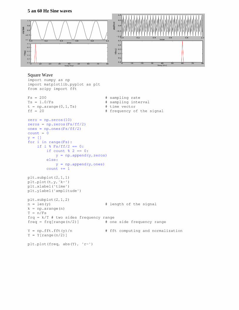
5 an 60 Hz Sine waves

Square Wave import numpy as np import matplotlib.pyplot as plt from scipy import fft Fs = 200 # sampling rate Ts = 1.0/Fs # sampling interva l t = np.arange(0,1,Ts) # time vector ff = 20 # frequency of the signal zero = np.zeros(10) zeros = np.zeros(Fs/ff/2) ones = np.ones(Fs/ff/2) count = 0 y = [] for i in range(Fs): if i % Fs/ff/2 == 0: if count % 2 == 0: y = np.append(y,zeros) else: y = np.append(y,ones) count += 1 plt.subplot(2,1,1) plt.plot(t,y,'k-') plt.xlabel('time') plt.ylabel('amplitude') plt.subplot(2,1,2) n = len(y) # length of the si gnal k = np.arange(n) T = n/Fs frq = k/T # two sides frequency range freq = frq[range(n/2)] # one side frequen cy range Y = np.fft.fft(y)/n # fft computing an d normalization Y = Y[range(n/2)] plt.plot(freq, abs(Y), 'r-')

5 Hz square wave:

import numpy as np import matplotlib.pyplot as plt from scipy import fft Fs = 200 # sampling rate Ts = 1.0/Fs # sampling interva l t = np.arange(0,1,Ts) # time vector ff = 5 # frequency of the signal nPulse = 20 y = np.ones(nPulse) y = np.append(y, np.zeros(Fs-nPulse)) plt.subplot(2,1,1) plt.plot(t,y,'k-') plt.xlabel('time') plt.ylabel('amplitude') plt.subplot(2,1,2) n = len(y) # length of the si gnal k = np.arange(n) T = n/Fs frq = k/T # two sides frequency range freq = frq[range(n/2)] # one side frequen cy range Y = np.fft.fft(y)/n # fft computing an d normalization Y = Y[range(n/2)] plt.plot(freq, abs(Y), 'r-') plt.xlabel('freq (Hz)') plt.ylabel('|Y(freq)|') plt.show()

Impulse (Unit pulse):

import numpy as np import matplotlib.pyplot as plt from scipy import fft Fs = 200 # sampling rate Ts = 1.0/Fs # sampling interva l t = np.arange(0,1,Ts) # time vector ff = 5 # frequency of the signal y = np.random.randn(Fs) plt.subplot(2,1,1) plt.plot(t,y,'k-') plt.xlabel('time') plt.ylabel('amplitude') plt.subplot(2,1,2) n = len(y) # length of the si gnal k = np.arange(n) T = n/Fs frq = k/T # two sides frequency range freq = frq[range(n/2)] # one side frequen cy range Y = np.fft.fft(y)/n # fft computing an d normalization Y = Y[range(n/2)] plt.plot(freq, abs(Y), 'r-') plt.xlabel('freq (Hz)') plt.ylabel('|Y(freq)|') plt.show()

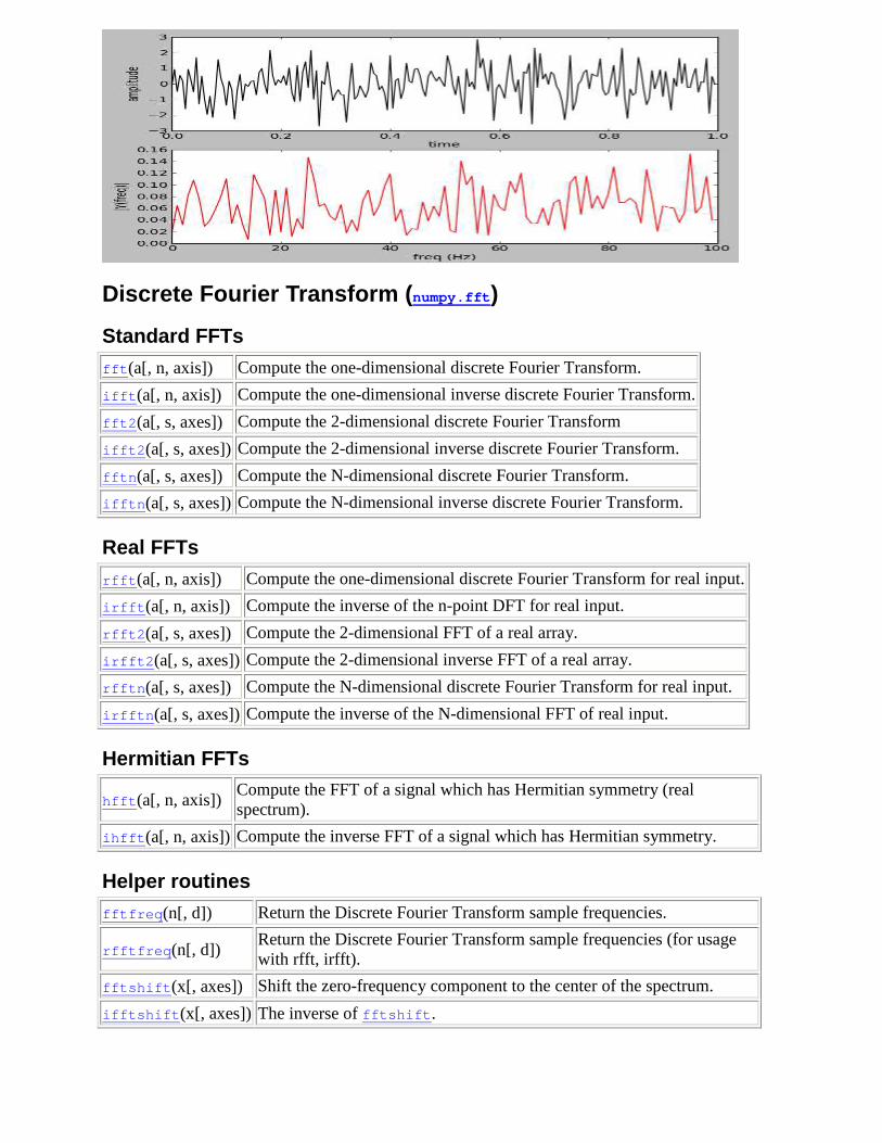
Discrete Fourier Transform (numpy.fft)

Standard FFTs

fft (a[, n, axis]) Compute the one-dimensional discrete Fourier Transform.

ifft (a[, n, axis]) Compute the one-dimensional inverse discrete Fourier Transform.

fft2 (a[, s, axes]) Compute the 2-dimensional discrete Fourier Transform

ifft2 (a[, s, axes]) Compute the 2-dimensional inverse discrete Fourier Transform.

fftn (a[, s, axes]) Compute the N-dimensional discrete Fourier Transform.

ifftn (a[, s, axes]) Compute the N-dimensional inverse discrete Fourier Transform.

Real FFTs

rfft (a[, n, axis]) Compute the one-dimensional discrete Fourier Transform for real input.

irfft (a[, n, axis]) Compute the inverse of the n-point DFT for real input.

rfft2 (a[, s, axes]) Compute the 2-dimensional FFT of a real array.

irfft2 (a[, s, axes]) Compute the 2-dimensional inverse FFT of a real array.

rfftn (a[, s, axes]) Compute the N-dimensional discrete Fourier Transform for real input.

irfftn (a[, s, axes]) Compute the inverse of the N-dimensional FFT of real input.

Hermitian FFTs

hfft (a[, n, axis]) Compute the FFT of a signal which has Hermitian symmetry (real spectrum).

ihfft (a[, n, axis]) Compute the inverse FFT of a signal which has Hermitian symmetry.

Helper routines

fftfreq (n[, d]) Return the Discrete Fourier Transform sample frequencies.

rfftfreq (n[, d]) Return the Discrete Fourier Transform sample frequencies (for usage with rfft, irfft).

fftshift (x[, axes]) Shift the zero-frequency component to the center of the spectrum.

ifftshift (x[, axes]) The inverse of fftshift .

Background information

Fourier analysis is fundamentally a method for expressing a function as a sum of periodic components, and for recovering the function from those components. When both the function and its Fourier transform are replaced with discretized counterparts, it is called the discrete Fourier transform (DFT). The DFT has become a mainstay of numerical computing in part because of a very fast algorithm for computing it, called the Fast Fourier Transform (FFT), which was known to Gauss (1805) and was brought to light in its current form by Cooley and Tukey [CT]. Press et al. [NR] provide an accessible introduction to Fourier analysis and its applications.

Because the discrete Fourier transform separates its input into components that contribute at discrete frequencies, it has a great number of applications in digital signal processing, e.g., for filtering, and in this context the discretized input to the transform is customarily referred to as a signal, which exists in the time domain. The output is called a spectrum or transform and exists in the frequency domain.

Implementation details

There are many ways to define the DFT, varying in the sign of the exponent, normalization, etc. In this implementation, the DFT is defined as

The DFT is in general defined for complex inputs and outputs, and a single-frequency component at linear frequency is represented by a complex exponential

, where is the sampling interval.

The values in the result follow so-called “standard” order: If A = fft(a, n) , then A[0] contains the zero-frequency term (the mean of the signal), which is always purely real for real inputs. Then A[1:n/2] contains the positive-frequency terms, and A[n/2+1:] contains the negative-frequency terms, in order of decreasingly negative frequency. For an even number of input points, A[n/2] represents both positive and negative Nyquist frequency, and is also purely real for real input. For an odd number of input points, A[(n-1)/2] contains the largest positive frequency, while A[(n+1)/2] contains the largest negative frequency. The routine np.fft.fftfreq(n) returns an array giving the frequencies of corresponding elements in the output. The routine np.fft.fftshift(A) shifts transforms and their frequencies to put the zero-frequency components in the middle, and np.fft.ifftshift(A) undoes that shift.

When the input a is a time-domain signal and A = fft(a) , np.abs(A) is its amplitude spectrum and np.abs(A)**2 is its power spectrum. The phase spectrum is obtained by np.angle(A) .

The inverse DFT is defined as

It differs from the forward transform by the sign of the exponential argument and the normalization by .

Real and Hermitian transforms

When the input is purely real, its transform is Hermitian, i.e., the component at frequency is the complex conjugate of the component at frequency , which means that for real inputs there is no information in the negative frequency components that is not already available from the positive frequency components. The family of rfft functions is designed to operate on real inputs, and exploits this symmetry by computing only the positive frequency components, up to and including the Nyquist frequency. Thus, n input points produce n/2+1 complex output points. The inverses of this family assumes the same symmetry of its input, and for an output of n points uses n/2+1 input points.

Correspondingly, when the spectrum is purely real, the signal is Hermitian. The hfft family of functions exploits this symmetry by using n/2+1 complex points in the input (time) domain for n real points in the frequency domain.

In higher dimensions, FFTs are used, e.g., for image analysis and filtering. The computational efficiency of the FFT means that it can also be a faster way to compute large convolutions, using the property that a convolution in the time domain is equivalent to a point-by-point multiplication in the frequency domain.

Higher dimensions

In two dimensions, the DFT is defined as

which extends in the obvious way to higher dimensions, and the inverses in higher dimensions also extend in the same way.

numpy.fft.fft numpy.fft.fft (a, n=None, axis=-1)

Compute the one-dimensional discrete Fourier Transform.

This function computes the one-dimensional n-point discrete Fourier Transform (DFT) with the efficient Fast Fourier Transform (FFT) algorithm [CT].

Parameters:

a : array_like

Input array, can be complex.

n : int, optional

Length of the transformed axis of the output. If n is smaller than the length of the input, the input is cropped. If it is larger, the input is padded with zeros. If n is not given, the length of the input along the axis specified by axis is used.

axis : int, optional

Axis over which to compute the FFT. If not given, the last axis is used.

Returns:

out : complex ndarray

The truncated or zero-padded input, transformed along the axis indicated by axis, or the last one if axis is not specified.

Raises: IndexError :

if axes is larger than the last axis of a.

See also

numpy.fft for definition of the DFT and conventions used. ifft The inverse of fft . fft2 The two-dimensional FFT. fftn The n-dimensional FFT. rfftn The n-dimensional FFT of real input. fftfreq Frequency bins for given FFT parameters.

Notes

FFT (Fast Fourier Transform) refers to a way the discrete Fourier Transform (DFT) can be calculated efficiently, by using symmetries in the calculated terms. The symmetry is highest when n is a power of 2, and the transform is therefore most efficient for these sizes.

The DFT is defined, with the conventions used in this implementation, in the documentation for the numpy.fft module.

References

[CT] Cooley, James W., and John W. Tukey, 1965, “An algorithm for the machine calculation of complex Fourier series,” Math. Comput. 19: 297-301.

Examples

>>>

>>> np.fft.fft(np.exp(2j * np.pi * np.arange(8) / 8 )) array([ -3.44505240e-16 +1.14383329e-17j, 8.00000000e+00 -5.71092652e-15j, 2.33482938e-16 +1.22460635e-16j, 1.64863782e-15 +1.77635684e-15j, 9.95839695e-17 +2.33482938e-16j, 0.00000000e+00 +1.66837030e-15j, 1.14383329e-17 +1.22460635e-16j, -1.64863782e-15 +1.77635684e-15j]) >>> >>> import matplotlib.pyplot as plt >>> t = np.arange(256) >>> sp = np.fft.fft(np.sin(t)) >>> freq = np.fft.fftfreq(t.shape[-1]) >>> plt.plot(freq, sp.real, freq, sp.imag) [<matplotlib.lines.Line2D object at 0x...>, <matplo tlib.lines.Line2D object at 0x...>] >>> plt.show()

In this example, real input has an FFT which is Hermitian, i.e., symmetric in the real part and anti-symmetric in the imaginary part, as described in the numpy.fft documentation.

numpy.fft.ifft numpy.fft.ifft (a, n=None, axis=-1)[source]

Compute the one-dimensional inverse discrete Fourier Transform.

This function computes the inverse of the one-dimensional n-point discrete Fourier transform computed by fft . In other words, ifft(fft(a)) == a to within numerical accuracy. For a general description of the algorithm and definitions, see numpy.fft .

The input should be ordered in the same way as is returned by fft , i.e., a[0] should contain the zero frequency term, a[1:n/2+1] should contain the positive-frequency terms, and a[n/2+1:] should contain the negative-frequency terms, in order of decreasingly negative frequency. See numpy.fft for details.

Parameters:

a : array_like


n : int, optional

Length of the transformed axis of the output. If n is smaller than the length of the input, the input is cropped. If it is larger, the input is padded with zeros. If n is not given, the length of the input along the axis specified by axis is used. See notes about padding issues.


Axis over which to compute the inverse DFT. If not given, the last axis is used.

Returns:


The truncated or zero-padded input, transformed along the axis indicated by axis, or the last one if axis is not specified.


If axes is larger than the last axis of a.

See also

numpy.fft An introduction, with definitions and general explanations. fft The one-dimensional (forward) FFT, of which ifft is the inverse ifft2 The two-dimensional inverse FFT. ifftn The n-dimensional inverse FFT.

Notes

If the input parameter n is larger than the size of the input, the input is padded by appending zeros at the end. Even though this is the common approach, it might lead to surprising results. If a different padding is desired, it must be performed before calling ifft .

Examples

>>> >>> np.fft.ifft([0, 4, 0, 0]) array([ 1.+0.j, 0.+1.j, -1.+0.j, 0.-1.j])

Create and plot a band-limited signal with random phases:

>>> >>> import matplotlib.pyplot as plt >>> t = np.arange(400) >>> n = np.zeros((400,), dtype=complex) >>> n[40:60] = np.exp(1j*np.random.uniform(0, 2*np. pi, (20,))) >>> s = np.fft.ifft(n) >>> plt.plot(t, s.real, 'b-', t, s.imag, 'r--') [<matplotlib.lines.Line2D object at 0x...>, <matplo tlib.lines.Line2D object at 0x...>] >>> plt.legend(('real', 'imaginary')) <matplotlib.legend.Legend object at 0x...>

numpy.fft.fft2 numpy.fft.fft2 (a, s=None, axes=(-2, -1))[source]

Compute the 2-dimensional discrete Fourier Transform

This function computes the n-dimensional discrete Fourier Transform over any axes in an M-dimensional array by means of the Fast Fourier Transform (FFT). By default, the transform is computed over the last two axes of the input array, i.e., a 2-dimensional FFT.

Parameters:

a : array_like

Input array, can be complex

s : sequence of ints, optional

Shape (length of each transformed axis) of the output (s[0] refers to axis 0, s[1] to axis 1, etc.). This corresponds to n for fft(x, n). Along each axis, if the given shape is smaller than that of the input, the input is cropped. If it is larger, the input is padded with zeros. if s is not given, the shape of the input along the axes specified by axes is used.

axes : sequence of ints, optional

Axes over which to compute the FFT. If not given, the last two axes are used. A repeated index in axes means the transform over that axis is performed multiple times. A one-element sequence means that a one-dimensional FFT is performed.

Returns:


The truncated or zero-padded input, transformed along the axes indicated by axes, or the last two axes if axes is not given.

Raises:

ValueError :

If s and axes have different length, or axes not given and len(s) != 2 .

IndexError :

If an element of axes is larger than than the number of axes of a.

See also

numpy.fft Overall view of discrete Fourier transforms, with definitions and conventions used. ifft2 The inverse two-dimensional FFT. fft The one-dimensional FFT. fftn The n-dimensional FFT. fftshift Shifts zero-frequency terms to the center of the array. For two-dimensional input, swaps first and third quadrants, and second and fourth quadrants.

Notes

fft2 is just fftn with a different default for axes.

The output, analogously to fft , contains the term for zero frequency in the low-order corner of the transformed axes, the positive frequency terms in the first half of these axes, the term for the Nyquist frequency in the middle of the axes and the negative frequency terms in the second half of the axes, in order of decreasingly negative frequency.

See fftn for details and a plotting example, and numpy.fft for definitions and conventions used.

Examples

>>> >>> a = np.mgrid[:5, :5][0] >>> np.fft.fft2(a) array([[ 50.0 +0.j , 0.0 +0.j , 0 .0 +0.j , 0.0 +0.j , 0.0 +0.j ], [-12.5+17.20477401j, 0.0 +0.j , 0 .0 +0.j , 0.0 +0.j , 0.0 +0.j ], [-12.5 +4.0614962j , 0.0 +0.j , 0 .0 +0.j , 0.0 +0.j , 0.0 +0.j ], [-12.5 -4.0614962j , 0.0 +0.j , 0 .0 +0.j , 0.0 +0.j , 0.0 +0.j ], [-12.5-17.20477401j, 0.0 +0.j , 0 .0 +0.j , 0.0 +0.j , 0.0 +0.j ]])

numpy.fft.ifft2

numpy.fft.ifft2 (a, s=None, axes=(-2, -1))[source]

Compute the 2-dimensional inverse discrete Fourier Transform.

This function computes the inverse of the 2-dimensional discrete Fourier Transform over any number of axes in an M-dimensional array by means of the Fast Fourier Transform (FFT). In other words, ifft2(fft2(a)) == a to within numerical accuracy. By default, the inverse transform is computed over the last two axes of the input array.

The input, analogously to ifft , should be ordered in the same way as is returned by fft2 , i.e. it should have the term for zero frequency in the low-order corner of the two axes, the positive frequency terms in the first half of these axes, the term for the Nyquist frequency in the middle of the axes and the negative frequency terms in the second half of both axes, in order of decreasingly negative frequency.

Parameters:

a : array_like



Shape (length of each axis) of the output (s[0] refers to axis 0, s[1] to axis 1, etc.). This corresponds to n for ifft(x, n) . Along each axis, if the given shape is smaller than that of the input, the input is cropped. If it is larger, the input is padded with zeros. if s is not given, the shape of the input along the axes specified by axes is used. See notes for issue on ifft zero padding.


Axes over which to compute the FFT. If not given, the last two axes are used. A repeated index in axes means the transform over that axis is performed multiple times. A one-element sequence means that a one-dimensional FFT is performed.

Returns:


The truncated or zero-padded input, transformed along the axes indicated by axes, or the last two axes if axes is not given.

Raises:

ValueError :

If s and axes have different length, or axes not given and len(s) != 2 .

IndexError :


See also

numpy.fft Overall view of discrete Fourier transforms, with definitions and conventions used. fft2 The forward 2-dimensional FFT, of which ifft2 is the inverse. ifftn The inverse of the n-dimensional FFT. fft The one-dimensional FFT. ifft The one-dimensional inverse FFT.

Notes

ifft2 is just ifftn with a different default for axes.

See ifftn for details and a plotting example, and numpy.fft for definition and conventions used.

Zero-padding, analogously with ifft , is performed by appending zeros to the input along the specified dimension. Although this is the common approach, it might lead to surprising results. If another form of zero padding is desired, it must be performed before ifft2 is called.

Examples

>>> >>> a = 4 * np.eye(4) >>> np.fft.ifft2(a) array([[ 1.+0.j, 0.+0.j, 0.+0.j, 0.+0.j], [ 0.+0.j, 0.+0.j, 0.+0.j, 1.+0.j], [ 0.+0.j, 0.+0.j, 1.+0.j, 0.+0.j], [ 0.+0.j, 1.+0.j, 0.+0.j, 0.+0.j]])

numpy.fft.fftn numpy.fft.fftn (a, s=None, axes=None)[source]

Compute the N-dimensional discrete Fourier Transform.

This function computes the N-dimensional discrete Fourier Transform over any number of axes in an M-dimensional array by means of the Fast Fourier Transform (FFT).

Parameters:

a : array_like



Shape (length of each transformed axis) of the output (s[0] refers to axis 0, s[1] to axis 1, etc.). This corresponds to n for fft(x, n). Along any axis, if the given shape is smaller than that of the input, the input is cropped. If it is larger, the input is padded with zeros. if s is not given, the shape of the input along the axes specified by axes is used.


Axes over which to compute the FFT. If not given, the last len(s) axes are used, or all axes if s is also not specified. Repeated indices in axes means that the transform over that axis is performed multiple times.

Returns:


The truncated or zero-padded input, transformed along the axes indicated by axes, or by a combination of s and a, as explained in the parameters section above.

Raises:

ValueError :

If s and axes have different length.

IndexError :


See also

numpy.fft Overall view of discrete Fourier transforms, with definitions and conventions used. ifftn The inverse of fftn , the inverse n-dimensional FFT. fft The one-dimensional FFT, with definitions and conventions used. rfftn The n-dimensional FFT of real input. fft2 The two-dimensional FFT. fftshift Shifts zero-frequency terms to centre of array

Notes

The output, analogously to fft , contains the term for zero frequency in the low-order corner of all axes, the positive frequency terms in the first half of all axes, the term for the Nyquist frequency in the middle of all axes and the negative frequency terms in the second half of all axes, in order of decreasingly negative frequency.

See numpy.fft for details, definitions and conventions used.

Examples

>>> >>> a = np.mgrid[:3, :3, :3][0] >>> np.fft.fftn(a, axes=(1, 2)) array([[[ 0.+0.j, 0.+0.j, 0.+0.j], [ 0.+0.j, 0.+0.j, 0.+0.j], [ 0.+0.j, 0.+0.j, 0.+0.j]], [[ 9.+0.j, 0.+0.j, 0.+0.j], [ 0.+0.j, 0.+0.j, 0.+0.j], [ 0.+0.j, 0.+0.j, 0.+0.j]], [[ 18.+0.j, 0.+0.j, 0.+0.j], [ 0.+0.j, 0.+0.j, 0.+0.j], [ 0.+0.j, 0.+0.j, 0.+0.j]]]) >>> np.fft.fftn(a, (2, 2), axes=(0, 1)) array([[[ 2.+0.j, 2.+0.j, 2.+0.j], [ 0.+0.j, 0.+0.j, 0.+0.j]], [[-2.+0.j, -2.+0.j, -2.+0.j], [ 0.+0.j, 0.+0.j, 0.+0.j]]]) >>> >>> import matplotlib.pyplot as plt >>> [X, Y] = np.meshgrid(2 * np.pi * np.arange(200) / 12, ... 2 * np.pi * np.arange(200) / 34) >>> S = np.sin(X) + np.cos(Y) + np.random.uniform(0 , 1, X.shape) >>> FS = np.fft.fftn(S) >>> plt.imshow(np.log(np.abs(np.fft.fftshift(FS))** 2)) <matplotlib.image.AxesImage object at 0x...> >>> plt.show()

numpy.fft.ifftn numpy.fft.ifftn (a, s=None, axes=None)[source]

Compute the N-dimensional inverse discrete Fourier Transform.

This function computes the inverse of the N-dimensional discrete Fourier Transform over any number of axes in an M-dimensional array by means of the Fast Fourier Transform (FFT). In other words, ifftn(fftn(a)) == a to within numerical accuracy. For a description of the definitions and conventions used, see numpy.fft .

The input, analogously to ifft , should be ordered in the same way as is returned by fftn , i.e. it should have the term for zero frequency in all axes in the low-order corner, the positive frequency terms in the first half of all axes, the term for the Nyquist frequency in the middle of all axes and the negative frequency terms in the second half of all axes, in order of decreasingly negative frequency.

Parameters:

a : array_like



Shape (length of each transformed axis) of the output (s[0] refers to axis 0, s[1] to axis 1, etc.). This corresponds to n for ifft(x, n) . Along any axis, if the given shape is smaller than that of the input, the input is cropped. If it is larger, the input is padded with zeros. if s is not given, the shape of the input along the axes specified by axes is used. See notes for issue on ifft zero padding.


Axes over which to compute the IFFT. If not given, the last len(s) axes are used, or all axes if s is also not specified. Repeated indices in axes means that the inverse transform over that axis is performed multiple times.

Returns:


The truncated or zero-padded input, transformed along the axes indicated by axes, or by a combination of s or a, as explained in the parameters section above.

Raises:

ValueError :


IndexError :


See also

numpy.fft Overall view of discrete Fourier transforms, with definitions and conventions used. fftn The forward n-dimensional FFT, of which ifftn is the inverse. ifft The one-dimensional inverse FFT. ifft2 The two-dimensional inverse FFT. ifftshift Undoes fftshift , shifts zero-frequency terms to beginning of array.

Notes

See numpy.fft for definitions and conventions used.

Zero-padding, analogously with ifft , is performed by appending zeros to the input along the specified dimension. Although this is the common approach, it might lead to surprising results. If another form of zero padding is desired, it must be performed before ifftn is called.

Examples

>>> >>> a = np.eye(4) >>> np.fft.ifftn(np.fft.fftn(a, axes=(0,)), axes=(1 ,)) array([[ 1.+0.j, 0.+0.j, 0.+0.j, 0.+0.j], [ 0.+0.j, 1.+0.j, 0.+0.j, 0.+0.j], [ 0.+0.j, 0.+0.j, 1.+0.j, 0.+0.j], [ 0.+0.j, 0.+0.j, 0.+0.j, 1.+0.j]])

Create and plot an image with band-limited frequency content:

>>> >>> import matplotlib.pyplot as plt >>> n = np.zeros((200,200), dtype=complex) >>> n[60:80, 20:40] = np.exp(1j*np.random.uniform(0 , 2*np.pi, (20, 20))) >>> im = np.fft.ifftn(n).real >>> plt.imshow(im) <matplotlib.image.AxesImage object at 0x...> >>> plt.show()

numpy.fft.rfft numpy.fft.rfft (a, n=None, axis=-1)[source]

Compute the one-dimensional discrete Fourier Transform for real input.

This function computes the one-dimensional n-point discrete Fourier Transform (DFT) of a real-valued array by means of an efficient algorithm called the Fast Fourier Transform (FFT).

Parameters:

a : array_like

Input array

n : int, optional

Number of points along transformation axis in the input to use. If n is smaller than the length of the input, the input is cropped. If it is larger, the input is padded with zeros. If n is not given, the length of the input along the axis specified by axis is used.


Axis over which to compute the FFT. If not given, the last axis is used.

Returns:


The truncated or zero-padded input, transformed along the axis indicated by axis, or the last one if axis is not specified. If n is even, the length of the transformed axis is (n/2)+1 . If n is odd, the length is (n+1)/2 .


If axis is larger than the last axis of a.

See also

numpy.fft For definition of the DFT and conventions used. irfft The inverse of rfft . fft The one-dimensional FFT of general (complex) input. fftn The n-dimensional FFT. rfftn The n-dimensional FFT of real input.

Notes

When the DFT is computed for purely real input, the output is Hermitian-symmetric, i.e. the negative frequency terms are just the complex conjugates of the corresponding positive-frequency terms, and the negative-frequency terms are therefore redundant. This function does not compute the negative frequency terms, and the length of the transformed axis of the output is therefore n//2 + 1 .

When A = rfft(a) and fs is the sampling frequency, A[0] contains the zero-frequency term 0*fs, which is real due to Hermitian symmetry.

If n is even, A[-1] contains the term representing both positive and negative Nyquist frequency (+fs/2 and -fs/2), and must also be purely real. If n is odd, there is no term at fs/2; A[-1] contains the largest positive frequency (fs/2*(n-1)/n), and is complex in the general case.

If the input a contains an imaginary part, it is silently discarded.

Examples

>>> >>> np.fft.fft([0, 1, 0, 0]) array([ 1.+0.j, 0.-1.j, -1.+0.j, 0.+1.j]) >>> np.fft.rfft([0, 1, 0, 0]) array([ 1.+0.j, 0.-1.j, -1.+0.j])

Notice how the final element of the fft output is the complex conjugate of the second element, for real input. For rfft , this symmetry is exploited to compute only the non-negative frequency terms.

numpy.fft.irfft numpy.fft.irfft (a, n=None, axis=-1)[source]

Compute the inverse of the n-point DFT for real input.

This function computes the inverse of the one-dimensional n-point discrete Fourier Transform of real input computed by rfft . In other words, irfft(rfft(a),

len(a)) == a to within numerical accuracy. (See Notes below for why len(a) is necessary here.)

The input is expected to be in the form returned by rfft , i.e. the real zero-frequency term followed by the complex positive frequency terms in order of increasing frequency. Since the discrete Fourier Transform of real input is Hermitian-symmetric, the negative frequency terms are taken to be the complex conjugates of the corresponding positive frequency terms.

Parameters:

a : array_like

The input array.

n : int, optional

Length of the transformed axis of the output. For n output points, n//2+1 input points are necessary. If the input is longer than this, it is cropped. If it is shorter than this, it is padded with zeros. If n is not given, it is determined from the length of the input along the axis specified by axis.


Axis over which to compute the inverse FFT. If not given, the last axis is

used.

Returns:

out : ndarray

The truncated or zero-padded input, transformed along the axis indicated by axis, or the last one if axis is not specified. The length of the transformed axis is n, or, if n is not given, 2*(m-1) where m is the length of the transformed axis of the input. To get an odd number of output points, n must be specified.


If axis is larger than the last axis of a.

See also

numpy.fft For definition of the DFT and conventions used. rfft The one-dimensional FFT of real input, of which irfft is inverse. fft The one-dimensional FFT. irfft2 The inverse of the two-dimensional FFT of real input. irfftn The inverse of the n-dimensional FFT of real input.

Notes

Returns the real valued n-point inverse discrete Fourier transform of a, where a contains the non-negative frequency terms of a Hermitian-symmetric sequence. n is the length of the result, not the input.

If you specify an n such that a must be zero-padded or truncated, the extra/removed values will be added/removed at high frequencies. One can thus resample a series to m points via Fourier interpolation by: a_resamp = irfft(rfft(a), m) .

Examples

>>> >>> np.fft.ifft([1, -1j, -1, 1j]) array([ 0.+0.j, 1.+0.j, 0.+0.j, 0.+0.j]) >>> np.fft.irfft([1, -1j, -1]) array([ 0., 1., 0., 0.])

Notice how the last term in the input to the ordinary ifft is the complex conjugate of the second term, and the output has zero imaginary part everywhere. When calling irfft , the negative frequencies are not specified, and the output array is purely real.

numpy.fft.rfft2 numpy.fft.rfft2 (a, s=None, axes=(-2, -1))[source]

Compute the 2-dimensional FFT of a real array.

Parameters:

a : array

Input array, taken to be real.


Shape of the FFT.


Axes over which to compute the FFT.

Returns: out : ndarray

The result of the real 2-D FFT.

See also

rfftn Compute the N-dimensional discrete Fourier Transform for real input.

Note: This is really just rfftn with different default behavior. For more details see rfftn .

numpy.fft.irfft2 numpy.fft.irfft2 (a, s=None, axes=(-2, -1))[source]

Compute the 2-dimensional inverse FFT of a real array.

Parameters:

a : array_like

The input array


Shape of the inverse FFT.


The axes over which to compute the inverse fft. Default is the last two axes.

Returns: out : ndarray

The result of the inverse real 2-D FFT.

See also

irfftn Compute the inverse of the N-dimensional FFT of real input.

Notes

This is really irfftn with different defaults. For more details see irfftn .

numpy.fft.rfftn numpy.fft.rfftn (a, s=None, axes=None)[source]

Compute the N-dimensional discrete Fourier Transform for real input.

This function computes the N-dimensional discrete Fourier Transform over any number of axes in an M-dimensional real array by means of the Fast Fourier Transform (FFT). By default, all axes are transformed, with the real transform performed over the last axis, while the remaining transforms are complex.

Parameters:

a : array_like

Input array, taken to be real.


Shape (length along each transformed axis) to use from the input. (s[0] refers to axis 0, s[1] to axis 1, etc.). The final element of s corresponds to n for rfft(x, n) , while for the remaining axes, it corresponds to n for fft(x, n) . Along any axis, if the given shape is smaller than that of the input, the input is cropped. If it is larger, the input is padded with zeros. if s is not given, the shape of the input along the axes specified by axes is used.


Axes over which to compute the FFT. If not given, the last len(s) axes are used, or all axes if s is also not specified.

Returns:


The truncated or zero-padded input, transformed along the axes indicated by axes, or by a combination of s and a, as explained in the parameters section above. The length of the last axis transformed will be s[-1]//2+1 , while the remaining transformed axes will have lengths according to s, or unchanged from the input.

Raises:

ValueError :


IndexError :


See also

irfftn The inverse of rfftn , i.e. the inverse of the n-dimensional FFT of real input. fft The one-dimensional FFT, with definitions and conventions used. rfft The one-dimensional FFT of real input. fftn The n-dimensional FFT. rfft2 The two-dimensional FFT of real input.

Notes

The transform for real input is performed over the last transformation axis, as by rfft , then the transform over the remaining axes is performed as by fftn . The order of the output is as for rfft for the final transformation axis, and as for fftn for the remaining transformation axes.

See fft for details, definitions and conventions used.

Examples

>>> >>> a = np.ones((2, 2, 2)) >>> np.fft.rfftn(a) array([[[ 8.+0.j, 0.+0.j], [ 0.+0.j, 0.+0.j]], [[ 0.+0.j, 0.+0.j], [ 0.+0.j, 0.+0.j]]]) >>> >>> np.fft.rfftn(a, axes=(2, 0)) array([[[ 4.+0.j, 0.+0.j], [ 4.+0.j, 0.+0.j]], [[ 0.+0.j, 0.+0.j], [ 0.+0.j, 0.+0.j]]])

numpy.fft.irfftn numpy.fft.irfftn (a, s=None, axes=None)[source]

Compute the inverse of the N-dimensional FFT of real input.

This function computes the inverse of the N-dimensional discrete Fourier Transform for real input over any number of axes in an M-dimensional array by means of the Fast Fourier Transform (FFT). In other words, irfftn(rfftn(a), a.shape) == a to within numerical accuracy. (The a.shape is necessary like len(a) is for irfft , and for the same reason.)

The input should be ordered in the same way as is returned by rfftn , i.e. as for irfft for the final transformation axis, and as for ifftn along all the other axes.

Parameters: a : array_like

Input array.


Shape (length of each transformed axis) of the output (s[0] refers to axis 0, s[1] to axis 1, etc.). s is also the number of input points used along this axis, except for the last axis, where s[-1]//2+1 points of the input are used. Along any axis, if the shape indicated by s is smaller than that of the input, the input is cropped. If it is larger, the input is padded with zeros. If s is not given, the shape of the input along the axes specified by axes is used.


Axes over which to compute the inverse FFT. If not given, the last len(s) axes are used, or all axes if s is also not specified. Repeated indices in axes means that the inverse transform over that axis is performed multiple times.

Returns:

out : ndarray

The truncated or zero-padded input, transformed along the axes indicated by axes, or by a combination of s or a, as explained in the parameters section above. The length of each transformed axis is as given by the corresponding element of s, or the length of the input in every axis except for the last one if s is not given. In the final transformed axis the length of the output when s is not given is 2*(m-1) where m is the length of the final transformed axis of the input. To get an odd number of output points in the final axis, s must be specified.

Raises:

ValueError :


IndexError :


See also

rfftn The forward n-dimensional FFT of real input, of which ifftn is the inverse. fft The one-dimensional FFT, with definitions and conventions used. irfft The inverse of the one-dimensional FFT of real input. irfft2 The inverse of the two-dimensional FFT of real input.

Notes

See fft for definitions and conventions used.

See rfft for definitions and conventions used for real input.

Examples

>>> >>> a = np.zeros((3, 2, 2)) >>> a[0, 0, 0] = 3 * 2 * 2 >>> np.fft.irfftn(a) array([[[ 1., 1.], [ 1., 1.]], [[ 1., 1.], [ 1., 1.]], [[ 1., 1.], [ 1., 1.]]])

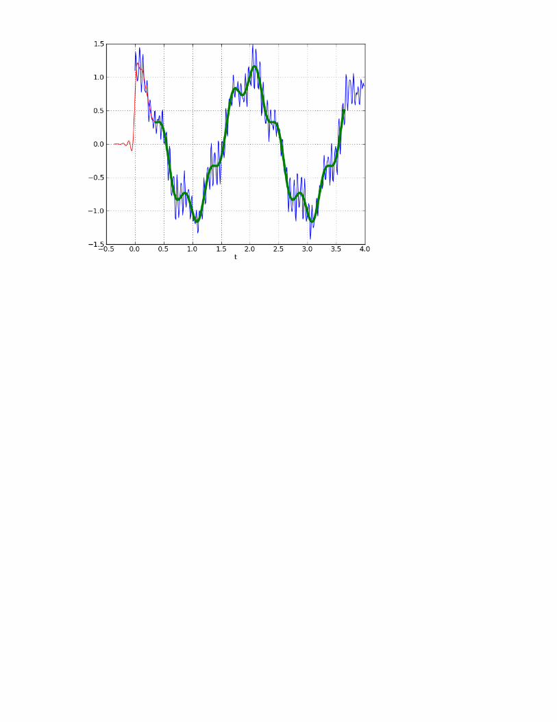
Example: FIR Filer #format wiki This cookbook example shows how to design and use a low-pass FIR filter using functions from scipy.signal. The pylab module from matplotlib is used to create plots. {{{ #!python from numpy import cos, sin, pi, absolute, arange from scipy.signal import kaiserord, lfilter, firwin , freqz from pylab import figure, clf, plot, xlabel, ylabel , xlim, ylim, title, grid, axes, show #------------------------------------------------ # Create a signal for demonstration. #------------------------------------------------ sample_rate = 100.0 nsamples = 400 t = arange(nsamples) / sample_rate x = cos(2*pi*0.5*t) + 0.2*sin(2*pi*2.5*t+0.1) + \ 0.2*sin(2*pi*15.3*t) + 0.1*sin(2*pi*16.7*t + 0.1) + \ 0.1*sin(2*pi*23.45*t+.8) #------------------------------------------------ # Create a FIR filter and apply it to x. #------------------------------------------------ # The Nyquist rate of the signal. nyq_rate = sample_rate / 2.0 # The desired width of the transition from pass to stop, # relative to the Nyquist rate. We'll design the f ilter # with a 5 Hz transition width. width = 5.0/nyq_rate # The desired attenuation in the stop band, in dB. ripple_db = 60.0 # Compute the order and Kaiser parameter for the FI R filter.

N, beta = kaiserord(ripple_db, width) # The cutoff frequency of the filter. cutoff_hz = 10.0 # Use firwin with a Kaiser window to create a lowpa ss FIR filter. taps = firwin(N, cutoff_hz/nyq_rate, window=('kaise r', beta)) # Use lfilter to filter x with the FIR filter. filtered_x = lfilter(taps, 1.0, x) #------------------------------------------------ # Plot the FIR filter coefficients. #------------------------------------------------ figure(1) plot(taps, 'bo-', linewidth=2) title('Filter Coefficients (%d taps)' % N) grid(True) #------------------------------------------------ # Plot the magnitude response of the filter. #------------------------------------------------ figure(2) clf() w, h = freqz(taps, worN=8000) plot((w/pi)*nyq_rate, absolute(h), linewidth=2) xlabel('Frequency (Hz)') ylabel('Gain') title('Frequency Response') ylim(-0.05, 1.05) grid(True) # Upper inset plot. ax1 = axes([0.42, 0.6, .45, .25]) plot((w/pi)*nyq_rate, absolute(h), linewidth=2) xlim(0,8.0) ylim(0.9985, 1.001) grid(True) # Lower inset plot ax2 = axes([0.42, 0.25, .45, .25]) plot((w/pi)*nyq_rate, absolute(h), linewidth=2) xlim(12.0, 20.0) ylim(0.0, 0.0025) grid(True) #------------------------------------------------ # Plot the original and filtered signals. #------------------------------------------------ # The phase delay of the filtered signal. delay = 0.5 * (N-1) / sample_rate figure(3) # Plot the original signal. plot(t, x) # Plot the filtered signal, shifted to compensate f or the phase delay. plot(t-delay, filtered_x, 'r-') # Plot just the "good" part of the filtered signal. The first N-1

# samples are "corrupted" by the initial conditions . plot(t[N-1:]-delay, filtered_x[N-1:], 'g', linewidt h=4) xlabel('t') grid(True) show() }}} The plots generated by the above code: attachment:fir_demo_taps.png attachment:fir_demo_freq_resp.png attachment:fir_demo_signals.png

Documents

Important sources for Numpy and Scipy Documentationhomes.ieu.edu.tr/skondakci/courses/CE476/frequency spectrum with scipy.pdf · Transform (FFT) is an efficient method for calculating