Import and Export of Spectra Files - The · PDF fileImport and Export of Spectra Files ... please send an email to ... labels a list with the proper labels

Import and Export of Spectra FilesVignette for the R package hyperSpec

Claudia Beleites <[email protected]>DIA Raman Spectroscopy Group, University of Trieste/Italy

Spectroscopy · Imaging, IPHT, Jena/Germany

June 30, 2017

hyperSpec supports a number of file formats relevant for different types of spectroscopy. This isnaturally only a subset of the file formats produced by different spectroscopic equipment.If you use hyperSpec with data formats not mentioned in this document, please send an email toClaudia Beleites <[email protected]>, so that this document can be updated.The information should include

• The type of spectroscopy

• Spectrometer model, manufacturer, and software

• The “native” file format (including a sample file)

• Description of relevant procedures to convert the file

• R code to import the data together with an example file that can actually be read by R.

• Documentation, particularly the description of the data format

If you need help finding out how to import your data, please search and eventually ask on Stack-exchange with tags [r] and [spectroscopy]. While I reqularly check these tags, consder dropping maClaudia Beleites <[email protected]>an email in addition.

Supported File Formats

The source code of this vignette including the spectra files are available as .zip file at hyperSpec’shome page: http://hyperspec.r-forge.r-project.org/blob/fileio.zipNote that some definitions are in file vignettes.defs.

Reproducing the Examples in this Vignette

Contents

1. Introduction 2

1

<[email protected]>

mailto:Claudia Beleites <[email protected]>

http://stackoverflow.com/questions/tagged/r+spectroscopy

http://stackoverflow.com/questions/tagged/r+spectroscopy


http://hyperspec.r-forge.r-project.org/blob/fileio.zip

2. Creating a hyperSpec object with new 32.1. Creating a hyperSpec Object from a Data Matrix (Spectra Matrix) . . . . . . . . . . . 32.2. Creating a hyperSpec Object from a Data Cube (Spectra Array) . . . . . . . . . . . . . 3

3. Reading Multiple files into one hyperSpec object 4

4. ASCII files 54.1. ASCII files with samples in columns . . . . . . . . . . . . . . . . . . . . . . . . . . . . . . 54.2. JCAMP-DX . . . . . . . . . . . . . . . . . . . . . . . . . . . . . . . . . . . . . . . . . . . . . 64.3. Basic Atomic Spectra from NIST Tables . . . . . . . . . . . . . . . . . . . . . . . . . . . . 74.4. Further ASCII Formats . . . . . . . . . . . . . . . . . . . . . . . . . . . . . . . . . . . . . . 84.5. ASCII Export . . . . . . . . . . . . . . . . . . . . . . . . . . . . . . . . . . . . . . . . . . . . 8

5. Binary file formats 85.1. Matlab Files . . . . . . . . . . . . . . . . . . . . . . . . . . . . . . . . . . . . . . . . . . . . . 8

5.1.1. Matlab Export . . . . . . . . . . . . . . . . . . . . . . . . . . . . . . . . . . . . . . . 95.1.2. Import of Matlab files written by Cytospec . . . . . . . . . . . . . . . . . . . . . 9

5.2. ENVI Files . . . . . . . . . . . . . . . . . . . . . . . . . . . . . . . . . . . . . . . . . . . . . 105.2.1. ENVI Export . . . . . . . . . . . . . . . . . . . . . . . . . . . . . . . . . . . . . . . 10

5.3. spc Files . . . . . . . . . . . . . . . . . . . . . . . . . . . . . . . . . . . . . . . . . . . . . . . 10

6. Manufacturer-Specific Discussion of File Import 146.1. Manufacturer Specific Import Functions . . . . . . . . . . . . . . . . . . . . . . . . . . . . 146.2. Bruker FT-IR Imaging . . . . . . . . . . . . . . . . . . . . . . . . . . . . . . . . . . . . . . 146.3. Nicolet FT-IR Imaging . . . . . . . . . . . . . . . . . . . . . . . . . . . . . . . . . . . . . . 146.4. Varian/Agilent FT-IR Imaging . . . . . . . . . . . . . . . . . . . . . . . . . . . . . . . . . 146.5. Kaiser Optical Systems Raman . . . . . . . . . . . . . . . . . . . . . . . . . . . . . . . . . 15

6.5.1. Kaiser Optical Systems ASCII Files . . . . . . . . . . . . . . . . . . . . . . . . . . 156.5.2. Kaiser Optical Systems Raman Maps . . . . . . . . . . . . . . . . . . . . . . . . . 15

6.6. Renishaw Raman . . . . . . . . . . . . . . . . . . . . . . . . . . . . . . . . . . . . . . . . . . 166.6.1. Renishaw ASCII data . . . . . . . . . . . . . . . . . . . . . . . . . . . . . . . . . . 16

6.7. Horiba / Jobin Yvon (e.g. LabRAM) . . . . . . . . . . . . . . . . . . . . . . . . . . . . . 176.8. Andor Solis . . . . . . . . . . . . . . . . . . . . . . . . . . . . . . . . . . . . . . . . . . . . . 176.9. Witec . . . . . . . . . . . . . . . . . . . . . . . . . . . . . . . . . . . . . . . . . . . . . . . . . 18

7. Writing your own Import Function 197.1. A new ASCII Import Function: scan.txt.PerkinElmer . . . . . . . . . . . . . . . . . . . . 197.2. Deriving a More Specific Function: read.ENVI.Nicolet . . . . . . . . . . . . . . . . . . . 217.3. Deriving import filters for spc files . . . . . . . . . . . . . . . . . . . . . . . . . . . . . . . 22

A. File Import Functions by Format 24

B. File Import Functions by Manufacturer 25

C. File Import Functions by Spectroscopy 26

D. Unit Test Results 26

1. Introduction

This document describes how spectra can be imported into hyperSpec objects. Some possibilities toexport hyperSpec objects as files are mentioned, too.

2

The most basic funtion to create hyperSpec objects is new ("hyperSpec") (section 2). It makes ahyperSpec object from data already in R’s workspace. Thus, once the spectra are imported into R,conversion to hyperSpec objects is straightforward.

In addition, hyperSpec comes with predifined import functions for different data formats. Thisdocument divides the discussion into dealing with ASCII files (section 4, p. 5) and binary file formats(section 5, p. 8). If data export for the respective format is possible, it is discussed in the samesections. As sometimes the actual data written by the spectrometer software exhibits peculiarities,hyperSpec offers several specialized import functions. These are in general named after the dataformat followed by the manufacturer (e. g. read.ENVI.Nicolet).

Overview lists of the directly supported file formats are in the appendix: sorted by file format(appendix A, p. 24), manufacturer (appendix B, p. 25), and by spectroscopy (appendix C, p. 26).

2. Creating a hyperSpec object with new

To create a hyperSpec object from data in R’s workspace, use:

> spc <- new ("hyperSpec", spc, wavelength, data, labels)

With the arguments:

spc the spectra matrix (may also be given as matrix inside column $spc of data)

wavelength the wavelength axis vector

data the extra data (possibly already including the spectra matrix in column spc)

labels a list with the proper labels. Do not forget the wavelength axis label in $.wavelength

and the spectral intensity axis label in $spc.

Thus, once your data is in R’s workspace, creating a hyperSpec object is easy. I suggest wrappingthe code to import your data and the line joining it into a hyperSpec object by your own importfunction. You are more than welcome to contribute such import code to hyperSpec. Secion 7, (p. 19)discusses examples of custom import functions.

2.1. Creating a hyperSpec Object from a Data Matrix (Spectra Matrix)

As spectra matices are the internal format of hyperSpec, the consructor can directly be used:

> spc <- new ("hyperSpec", spc, wavelength, data, labels)

2.2. Creating a hyperSpec Object from a Data Cube (Spectra Array)

Roberto Moscetti asked how to convert a hyperspectral data cube into a hyperSpec object:

The problem is that I have a hypercube with the following dimensions: 67×41×256 y = 67

x = 41

w avel eng ths = 256

I do not know the way to import the hypercube.

Data cubes (i.e. 3-dimensional arrays of spectral data) result from spectal imaging measurements,where spectra are supplied for each pixel of an px.x ×px.y imaging area. They have 3 directions,usually x, y , and the spectral dimension.

The solution is to convert the array into a spectra matrix and have separate x and y coordinates.

Assume data is the data cube, and x, y and wl hold vectors with the proper x and y coordinatesand the wavelengths:

3

> data <- array (1 : 24, 4 : 2)

> wl <- c (550, 630)

> x <- c (1000, 1200, 1400)

> y <- c (1800, 1600, 1400, 1200)

> data

, , 1

[,1] [,2] [,3]

[1,] 1 5 9

[2,] 2 6 10

[3,] 3 7 11

[4,] 4 8 12

, , 2

[,1] [,2] [,3]

[1,] 13 17 21

[2,] 14 18 22

[3,] 15 19 23

[4,] 16 20 24

Such data can be converted into a hyperSpec object by:

> d <- dim (data)

> dim (data) <- c (d [1] * d [2], d [3])

> x <- rep (x, each = d [1])

> y <- rep (y, d [2])

> spectra <- new ("hyperSpec", spc = data,

+ data = data.frame (x, y), wavelength = wl)

If no proper coordinates (vectors x, y and wl) are available, they can be left out. In the case of xand y , map plotting will then be impossible, missing wavelengths will be replaced by column indicescounting from 1 to d [3] automatically. Of course, such sequences (the row/column/pixel numbers)can be used instead of the original x and y as well:

> y <- seq_len (d [1])

> x <- seq_len (d [2])

Data cubes often come from spectral imaging systems that use an“image”coordinate system countingy from top to bottom. Note that this should accounted for in the decreasing order of the original yvector.

3. Reading Multiple files into one hyperSpec object

Many of the function described below will work on one file, even though derived functions such asread.spc.KaiserMap (see section 6.5.2, p. 15) may take care of measurements consisting of multiplefiles.

Usually, the most convenient way to import multiple files into one hyperSpec object is reading allfiles into a list of hyperSpec objects, and then collapseing this list into a single hyperSpec object:

> files <- Sys.glob ("spc.Kaisermap/*.spc")

> files <- files [seq (1, length (files), by = 2)] # import low wavenumber region only

> spc <- lapply (files, read.spc)

> length (spc)

[1] 54

> spc [[1]]

4

hyperSpec object

1 spectra

4 data columns

1340 data points / spectrum

wavelength: x/"a. u." [numeric] 1 2 ... 1340

data: (1 rows x 4 columns)

1. z: x/"a. u." [numeric] 1

2. z.end: x/"a. u." [numeric] 1

3. spc: Counts [matrix1340] 2782.7 2229.8 ... 932.02

4. filename: filename [character] spc.Kaisermap/ebroAVII.spc

> spc <- collapse (spc)

> spc

hyperSpec object

54 spectra

4 data columns




1. z: x/"a. u." [numeric] 1 1 ... 1

2. z.end: x/"a. u." [numeric] 1 1 ... 1


4. filename: filename [character] spc.Kaisermap/ebroAVII.spc spc.Kaisermap/ebroAVIK.spc ... spc.Kaisermap/ebroAVXB.spc

Note that in this particular case, the spectra are more efficiently read by read.spc.KaiserMap (seesection 6.5.2, p. 15).

If you regularly import huge maps or images, writing a customized import function is highly en-couraged. You may gain speed and memory by using the internal workhorse functions for thefile import. In that case, please contact the package maintainer (Claudia Beleites <chemome-

[email protected]>) for advise (contributions to hyperSpec are welcome and all authors are listedappropriately in the function help page’s author section).

4. ASCII files

Currently, hyperSpec provides two functions for general ASCII data import:

read.txt.long imports long format ASCII files, i. e. one intensity value per row

read.txt.wide imports wide format ASCII files, i. e. one spectrum per row

The import functions immediately return a hyperSpec object.

Internally, they use read.table, a very powerful ASCII import function. R supplies another ASCIIimport function, scan. scan imports numeric data matrices and is faster than read.table, butcannot import column names. If your data does not contain a header or it is not important and cansafely be skipped, you may want to import your data using scan.

Note that R allows to use a variety of compressed file formats directly as ASCII files (for example, seesection 6.6.1 on p. 16). Also, both read.txt.long and read.txt.wide accept connections insteadof file names.

4.1. ASCII files with samples in columns

Richard Pena asked about importing another ASCII file type:

5



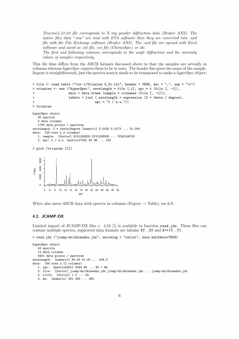
Triazine5 31.txt file corresponds to X ray powder diffraction data (Bruker AXS). Thenative files data “.raw” are read with EVA software then they are converted into .uxdfile with the File Exchange software (Bruker AXS). The .uxd file are opened with Excelsoftware and saved as .txt file, csv file (ChemoSpec) or xls.The first and following columns corresponds to the angle diffraction and the intensityvalues of samples respectively.

This file thus differs from the ASCII formats discussed above in that the samples are actually incolumns whereas hyperSpec expects them to be in rows. The header line gives the name of the sample.Import is straightforward, just the spectra matrix needs to be transposed to make a hyperSpec object:

> file <- read.table ("txt.t/Triazine 5_31.txt", header = TRUE, dec = ",", sep = "\t")

> triazine <- new ("hyperSpec", wavelength = file [,1], spc = t (file [, -1]),

+ data = data.frame (sample = colnames (file [, -1])),

+ labels = list (.wavelength = expression (2 * theta / degree),

+ spc = "I / a.u."))

> triazine

hyperSpec object

25 spectra

2 data columns


wavelength: 2 * theta/degree [numeric] 5.0025 5.0173 ... 31.004


1. sample: [factor] DIV1208200 DIV1208300 ... VCA0106703

2. spc: I / a.u. [matrix1759] 92 96 ... 163

> plot (triazine [1])

4 6 8 10 12 14 16 18 20 22 24 26 28 30 32

02

00

04

00

06

00

0

2θ °

I /

a.u

.I

/ a

.u.

Witec also saves ASCII data with spectra in columns (Export → Table), see 6.9.

4.2. JCAMP-DX

Limited import of JCAMP-DX files v. 4.24 [1] is available in function read.jdx. These files cancontain multiple spectra, supported data formats are tabular XY..XY and X++(Y..Y).

> read.jdx ("jcamp-dx/shimadzu.jdx", encoding = "latin1", keys.hdr2data=TRUE)

hyperSpec object

44 spectra

12 data columns


wavelength: [numeric] 60.05 61.05 ... 548.3


1. spc: [matrix3401] 3294 NA ... 90 + NA

2. file: [factor] jcamp-dx/shimadzu.jdx jcamp-dx/shimadzu.jdx ... jcamp-dx/shimadzu.jdx

3. title: [factor] 1 2 ... 44

4. mw: [numeric] 261 249 ... 382

6

5. molform: [factor] C11 H27 N O2 Si2 C9 H23 N O3 Si2 ... C25 H50 O2

6. casregistryno: [factor] 72 - 18 - 4 56 - 45 - 1 ... 2442 - 49 - 1

7. datatype: [factor] Mass Spectrum Mass Spectrum ... Mass Spectrum

8. sampledescription: [factor] ...\11-12-12\pAS+OS Lauf1.qgd"\n20000 Da/s, ET 30ms, m/z 60-550\nPeak-Apex-Spektrum, Hi

9. casname: [factor] L-Valin N,O-TMS2 L-Serin O,O'-TMS2 (X) ... Methyltetracosanoat (LRI C24)

10. $retentionindex: [numeric] 884 925 ... 2400

11. .format: [factor] (XY..XY) (XY..XY) ... (XY..XY)

12. filename: filename [character] jcamp-dx/shimadzu.jdx jcamp-dx/shimadzu.jdx ... jcamp-dx/shimadzu.jdx

> read.jdx ("jcamp-dx/virgilio.jdx")

hyperSpec object

1 spectra

2 data columns


wavelength: tilde(nu)/cm^-1 [numeric] 3030 3028 ... 600


1. spc: A [matrix1216] -3.1244e-05 0.0000e+00 ... 0

2. filename: filename [character] jcamp-dx/virgilio.jdx

The last file has a slight inconsistenty between its meta data and spectroscopic data, causing amessage. However, the difference is minute compared to the intensities. If this is known in advance,an appropriate tolerance can be chosen:

> read.jdx ("jcamp-dx/virgilio.jdx", ytol = 1e-9)

hyperSpec object

1 spectra

2 data columns


wavelength: tilde(nu)/cm^-1 [numeric] 3030 3028 ... 600


1. spc: A [matrix1216] -3.1244e-05 0.0000e+00 ... 0

2. filename: filename [character] jcamp-dx/virgilio.jdx

read.jdx.Shimadzu is deprecated.

Note

An R package dedicated to importing JCAMP-DX is currently under development by Bryan Hanson(https://github.com/bryanhanson/readJDX). hyperSpec will use that package once it is availableon CRAN. Maintenance of hyperSpec’s read.jdx function is limited from now on in favor of Bryan’spacakge.

Note

4.3. Basic Atomic Spectra from NIST Tables

The NIST (National Institute of Standards and Technology) has published a data base of basic atomicemission spectra (see http://physics.nist.gov/PhysRefData/Handbook/periodictable.htm)[?] with emission lines tabulated in ASCII (HTML) files.

Here’s an example how to extract the data of the Hg strong lines file:

> file <- readLines("NIST/mercurytable2.htm")

> #file <- readLines("http://physics.nist.gov/PhysRefData/Handbook/Tables/mercurytable2.htm")

>

> file <- file [- (1 : grep ("Intensity.*Wavelength", file) - 1)]

> file <- file [1 : (grep ("</pre>", file) [1] - 1)]

> file <- gsub ("<[^>]*>", "", file)

7

https://github.com/bryanhanson/readJDX

http://physics.nist.gov/PhysRefData/Handbook/periodictable.htm

> file <- file [! grepl ("^[[:space:]]+$", file)]

> colnames <- file [1]

> colnames <- gsub ("[[:space:]][[:space:]]+", "\t", file [1])

> colnames <- strsplit (colnames, "\t")[[1]]

> if (! all (colnames == c ("Intensity", "Wavelength (Å)", "Spectrum", "Ref. ")))

+ stop ("file format changed!")

> tablestart <- grep ("^[[:blank:]]*[[:alpha:]]+$", file) + 1

> tableend <- c (tablestart [-1] - 2, length (file))

> tables <- list ()

> for (t in seq_along (tablestart)){

+ tmp <- file [tablestart [t] : tableend [t]]

+ tables [[t]] <- read.fwf (textConnection (tmp), c (5, 8, 12, 15, 9))

+ colnames (tables [[t]]) <- c("Intensity", "persistent", "Wavelength", "Spectrum", "Ref. ")

+ tables [[t]]$type <- gsub ("[[:space:]]", "", file [tablestart [t] - 1])

+ }

> tables <- do.call (rbind, tables)

> levels (tables$Spectrum) <- gsub (" ", "", levels (tables$Spectrum))

> Hg.AES <- list ()

> for (s in levels (tables$Spectrum))

+ Hg.AES [[s]] <- new ("hyperSpec", wavelength = tables$Wavelength [tables$Spectrum == s],

+ spc = tables$Intensity [tables$Spectrum == s],

+ data = data.frame (Spectrum = s),

+ label = list (.wavelength = expression (lambda / ring (A)),

+ spc = "I"))

> plot (collapse (Hg.AES), lines.args = list (type = "h"), col = 1 : 2)

4.4. Further ASCII Formats

Further import filters are provided for manufacturer/software specific ASCII formats, see table A(p. 24) and section 6.1 (p. 14).

4.5. ASCII Export

ASCII export can be done in wide and long format using write.txt.long and write.txt.wide. Ifyou need a specific header or footer, use R’s functions for writing files: write.table, write, catand so on offer fine-grained control of writing ASCII files.

5. Binary file formats

5.1. Matlab Files

Matlab files can be read and written using the package R.matlab[2], which is available at CRAN andcan be installed by install.packages ("R.matlab").

spc.mat <- readMat ("spectra.mat")

If the .mat file was saved with compression, the additional package Rcompression is needed. It canbe installed from omegahat:

install.packages("Rcompression", repos = "http://www.omegahat.org/R")

See the documentation of R.matlab for more details and possibly needed further packages.

readMat imports the .mat file’s contents as a list. The variables in the .mat file are properly namedelements of the list. The hyperSpec object can be created using new, see 2 (p. 3).

Again, you probably want to wrap the import of your matlab files into a function.

8

5.1.1. Matlab Export

R.matlab’s function writeMat can be used to write R objects into .mat files. To save an hyperSpecobject x for use in Matlab, you most likely want to save:

• the wavelength axis as obtained by wl (x),

• the spectra matrix as obtained by x [[]], and

• possibly also the extra data as obtained by x$..

• as well as the axis labels labels (x).

• Alternatively, x$. yields the extra data together with the spectra matrix.

However, it may be convenient to transform the saved data according to how it is needed in Matlab.The functions as.long.df and as.wide.df may prove useful for reshaping the data.

5.1.2. Import of Matlab files written by Cytospec

A custom import function for .mat files written by Cytospec is available:

Note that Cytospec files can contain multiple versions of the data, the so-called blocks. The blockto be read can be specified with the block argument. TRUE will read all blocks into a list:

> read.mat.Cytospec ("mat.cytospec/cytospec.mat", blocks = TRUE)

[[1]]

hyperSpec object

55 spectra

5 data columns


wavelength: [numeric] 499.12 501.77 ... 3100


1. x: [integer] 4 5 ... 7

2. y: [integer] 1 1 ... 11

3. block: [integer] 1 1 ... 1

4. spc: [matrix981] 2112.9 2114.3 ... 2323.3

5. filename: filename [character] mat.cytospec/cytospec.mat mat.cytospec/cytospec.mat ... mat.cytospec/cytospec.mat

[[2]]

hyperSpec object

55 spectra

5 data columns




1. x: [integer] 4 5 ... 7

2. y: [integer] 1 1 ... 11


4. spc: [matrix981] 58.472 59.024 ... 262.5


otherwise, select a block:

> read.mat.Cytospec ("mat.cytospec/cytospec.mat", blocks = 1)

hyperSpec object

55 spectra

5 data columns




1. x: [integer] 4 5 ... 7

9

www.cytospec.com

2. y: [integer] 1 1 ... 11


4. spc: [matrix981] 2112.9 2114.3 ... 2323.3


read.cytomat has been renamed to read.mat.Cytospec to be more consistent with the generalnaming scheme of the file import functions.Please use read.mat.Cytospec instead.

read.cytomat is deprecated.

5.2. ENVI Files

ENVI files are binary data accompanied by an ASCII header file. hyperSpec’s function read.ENVI

can be used to import them. Usually, the header file name is the same as the binary data filename with the suffix replaced by .hdr. Otherwise, the header file name can be given via parameterheaderfile .

As we experienced missing header files (Bruker’s Opus software frequently produced header fileswithout any content), the data that would usually be read from the header file can also be handed toread.ENVI as a list in parameter header . Arguments given in header replace corresponding entriesof the header file. The help page gives details on what elements the list should contain, see also thediscussion of ENVI files written by Bruker’s OPUS software (section 6.2, p. 14).

Here is how to use read.ENVI:

> spc <- read.ENVI ("ENVI/example2.img")

> spc

hyperSpec object

0 spectra

3 data columns




1. x: [integer]

2. y: [integer]

3. spc: [matrix1738]

Please see also the manufacturer specific notes in section 6.1, p. 14.

Unit Tests

read.ENVI:

5.2.1. ENVI Export

Use package caTools or rgdal with GDAL for writing ENVI files.

5.3. spc Files

Thermo Galactic’s .spc file format can be imported by read.spc.

10

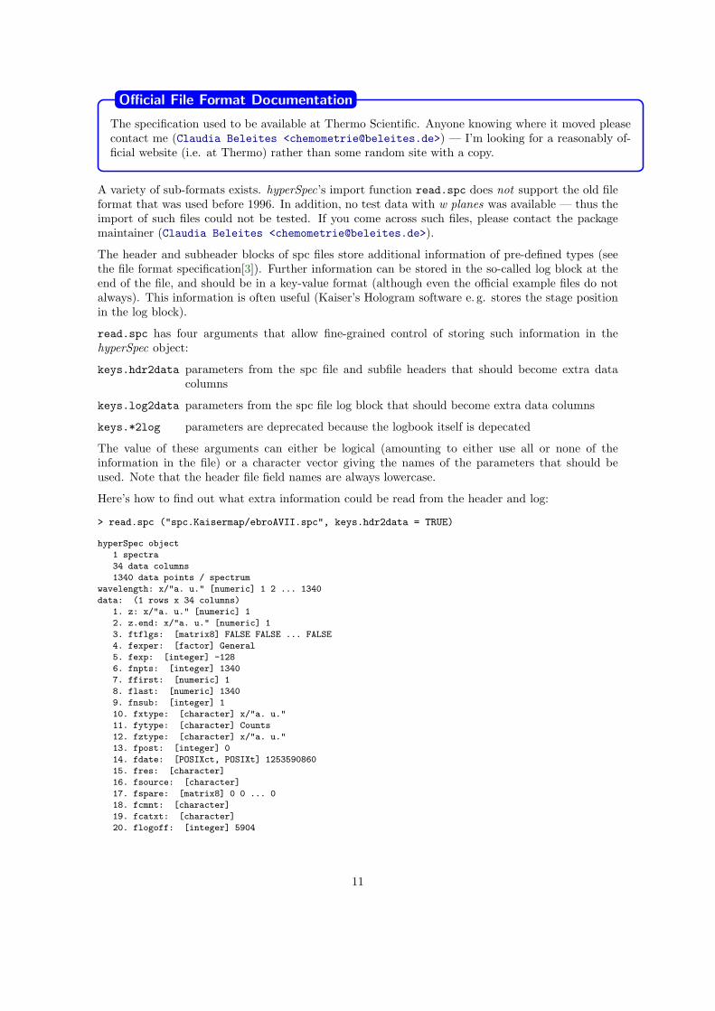
The specification used to be available at Thermo Scientific. Anyone knowing where it moved pleasecontact me (Claudia Beleites <[email protected]>) — I’m looking for a reasonably of-ficial website (i.e. at Thermo) rather than some random site with a copy.

Official File Format Documentation

A variety of sub-formats exists. hyperSpec’s import function read.spc does not support the old fileformat that was used before 1996. In addition, no test data with w planes was available — thus theimport of such files could not be tested. If you come across such files, please contact the packagemaintainer (Claudia Beleites <[email protected]>).

The header and subheader blocks of spc files store additional information of pre-defined types (seethe file format specification[3]). Further information can be stored in the so-called log block at theend of the file, and should be in a key-value format (although even the official example files do notalways). This information is often useful (Kaiser’s Hologram software e. g. stores the stage positionin the log block).

read.spc has four arguments that allow fine-grained control of storing such information in thehyperSpec object:

keys.hdr2data parameters from the spc file and subfile headers that should become extra datacolumns

keys.log2data parameters from the spc file log block that should become extra data columns

keys.*2log parameters are deprecated because the logbook itself is depecated

The value of these arguments can either be logical (amounting to either use all or none of theinformation in the file) or a character vector giving the names of the parameters that should beused. Note that the header file field names are always lowercase.

Here’s how to find out what extra information could be read from the header and log:

> read.spc ("spc.Kaisermap/ebroAVII.spc", keys.hdr2data = TRUE)

hyperSpec object

1 spectra

34 data columns






3. ftflgs: [matrix8] FALSE FALSE ... FALSE

4. fexper: [factor] General

5. fexp: [integer] -128

6. fnpts: [integer] 1340

7. ffirst: [numeric] 1

8. flast: [numeric] 1340

9. fnsub: [integer] 1

10. fxtype: [character] x/"a. u."

11. fytype: [character] Counts

12. fztype: [character] x/"a. u."

13. fpost: [integer] 0

14. fdate: [POSIXct, POSIXt] 1253590860

15. fres: [character]

16. fsource: [character]

17. fspare: [matrix8] 0 0 ... 0

18. fcmnt: [character]

19. fcatxt: [character]

20. flogoff: [integer] 5904

11



21. fmods: [integer] 0

22. fprocs: [integer] 0

23. flevel: [integer] 0

24. fsampin: [integer] 0

25. ffactor: [numeric] 0

26. fmethod: [character]

27. fzinc: [numeric] 0

28. fwplanes: [integer] 0

29. fwinc: [numeric] 0

30. fwtype: [character] x/"a. u."

31. .last.read: [numeric] 512

32. subfiledir: [numeric] 0



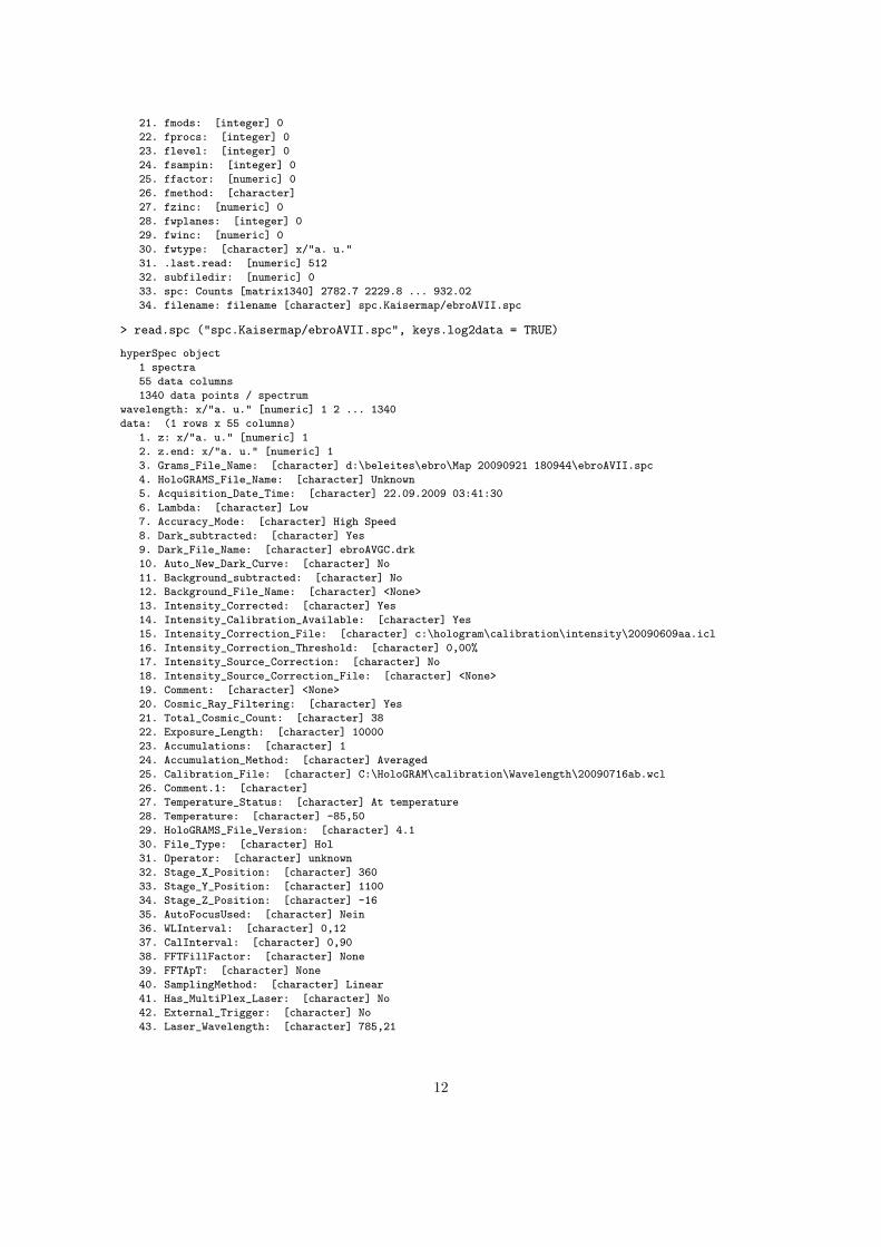
> read.spc ("spc.Kaisermap/ebroAVII.spc", keys.log2data = TRUE)

hyperSpec object

1 spectra

55 data columns






3. Grams_File_Name: [character] d:\beleites\ebro\Map 20090921 180944\ebroAVII.spc

4. HoloGRAMS_File_Name: [character] Unknown

5. Acquisition_Date_Time: [character] 22.09.2009 03:41:30

6. Lambda: [character] Low

7. Accuracy_Mode: [character] High Speed

8. Dark_subtracted: [character] Yes

9. Dark_File_Name: [character] ebroAVGC.drk

10. Auto_New_Dark_Curve: [character] No

11. Background_subtracted: [character] No

12. Background_File_Name: [character] <None>

13. Intensity_Corrected: [character] Yes

14. Intensity_Calibration_Available: [character] Yes

15. Intensity_Correction_File: [character] c:\hologram\calibration\intensity\20090609aa.icl

16. Intensity_Correction_Threshold: [character] 0,00%

17. Intensity_Source_Correction: [character] No

18. Intensity_Source_Correction_File: [character] <None>

19. Comment: [character] <None>

20. Cosmic_Ray_Filtering: [character] Yes

21. Total_Cosmic_Count: [character] 38

22. Exposure_Length: [character] 10000

23. Accumulations: [character] 1

24. Accumulation_Method: [character] Averaged

25. Calibration_File: [character] C:\HoloGRAM\calibration\Wavelength\20090716ab.wcl

26. Comment.1: [character]

27. Temperature_Status: [character] At temperature

28. Temperature: [character] -85,50

29. HoloGRAMS_File_Version: [character] 4.1

30. File_Type: [character] Hol

31. Operator: [character] unknown

32. Stage_X_Position: [character] 360

33. Stage_Y_Position: [character] 1100

34. Stage_Z_Position: [character] -16

35. AutoFocusUsed: [character] Nein

36. WLInterval: [character] 0,12

37. CalInterval: [character] 0,90

38. FFTFillFactor: [character] None

39. FFTApT: [character] None

40. SamplingMethod: [character] Linear

41. Has_MultiPlex_Laser: [character] No

42. External_Trigger: [character] No

43. Laser_Wavelength: [character] 785,21

12

44. Default_Laser_Wavelength: [character] 785,21

45. Laser_Tracking: [character] False

46. Laser_Block_Active: [character] No

47. Pixel_Fill_minimum: [character] 26

48. Pixel_Fill_maximum: [character] 16762

49. Binning_Start: [character] 24

50. Binning_End: [character] 41

51. NumPoints: [character] 1340

52. First: [character] 1,000

53. last: [character] 1340,000



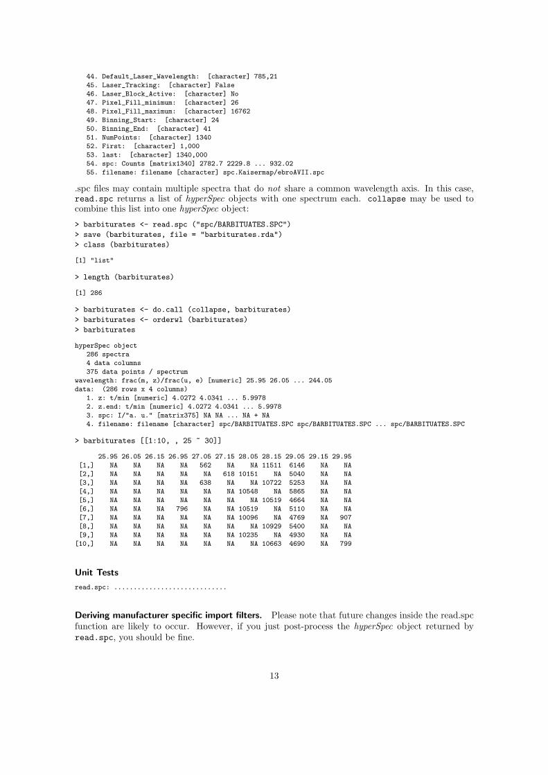
.spc files may contain multiple spectra that do not share a common wavelength axis. In this case,read.spc returns a list of hyperSpec objects with one spectrum each. collapse may be used tocombine this list into one hyperSpec object:

> barbiturates <- read.spc ("spc/BARBITUATES.SPC")

> save (barbiturates, file = "barbiturates.rda")

> class (barbiturates)

[1] "list"

> length (barbiturates)

[1] 286

> barbiturates <- do.call (collapse, barbiturates)

> barbiturates <- orderwl (barbiturates)

> barbiturates

hyperSpec object

286 spectra

4 data columns


wavelength: frac(m, z)/frac(u, e) [numeric] 25.95 26.05 ... 244.05


1. z: t/min [numeric] 4.0272 4.0341 ... 5.9978

2. z.end: t/min [numeric] 4.0272 4.0341 ... 5.9978

3. spc: I/"a. u." [matrix375] NA NA ... NA + NA

4. filename: filename [character] spc/BARBITUATES.SPC spc/BARBITUATES.SPC ... spc/BARBITUATES.SPC

> barbiturates [[1:10, , 25 ~ 30]]

25.95 26.05 26.15 26.95 27.05 27.15 28.05 28.15 29.05 29.15 29.95

[1,] NA NA NA NA 562 NA NA 11511 6146 NA NA

[2,] NA NA NA NA NA 618 10151 NA 5040 NA NA

[3,] NA NA NA NA 638 NA NA 10722 5253 NA NA

[4,] NA NA NA NA NA NA 10548 NA 5865 NA NA

[5,] NA NA NA NA NA NA NA 10519 4664 NA NA

[6,] NA NA NA 796 NA NA 10519 NA 5110 NA NA

[7,] NA NA NA NA NA NA 10096 NA 4769 NA 907

[8,] NA NA NA NA NA NA NA 10929 5400 NA NA

[9,] NA NA NA NA NA NA 10235 NA 4930 NA NA

[10,] NA NA NA NA NA NA NA 10663 4690 NA 799

Unit Tests

read.spc: .............................

Deriving manufacturer specific import filters. Please note that future changes inside the read.spcfunction are likely to occur. However, if you just post-process the hyperSpec object returned byread.spc, you should be fine.

13

6. Manufacturer-Specific Discussion of File Import

6.1. Manufacturer Specific Import Functions

Many spectrometer manufacturers provide a function to export their spectra into ASCII files. Thefunctions discussed above are written in a very general way, and are highly customizable. I rec-ommend wrapping these calls with the appropriate settings for your spectra format in an importfunction. Please consider contributing such import filters to hyperSpec: send me the documentedcode (for details see the box at the beginning of this document). If you are able to import data ofany format not mentioned in this document (even without the need of new converters), please letme know (details again in the box at the beginning of this document).

6.2. Bruker FT-IR Imaging

We use read.ENVI to import IR-Images collected with a Bruker Hyperion spectrometer with OPUSsoftware. As mentioned above, the header files are frequently empty. We found the necessaryinformation to be:

> header <- list (samples = 64 * no.images.in.row,

+ lines = 64 * no.images.in.column,

+ bands = no.data.points.per.spectrum,

+ `data type` = 4,

+ interleave = "bip")

No spatial information is given in the ENVI header (if written). The lateral coordinates can be setupby specifying origin and pixel size for x and y directions. For details please see the help page.

The proprietary file format of the Opus software is not yet supported.

6.3. Nicolet FT-IR Imaging

Also Nicolet saves imaging data in ENVI files. These files use some non-standard keywords in theheader file that should allow to reconstruct the lateral coordinates as well as the wavelength axes andunits for wavelength and intensity axis. hyperSpec has a specialized function read.ENVI.Nicolet

that uses these header entries.

It seems that the position of the first spectrum is recorded in µm, while the pixel size is in mm. Thusa flag nicolet.correction is provided that divides the pixel size by 1000. Alternatively, the correctoffset and pixel size values may be given as function arguments.

> spc <- read.ENVI.Nicolet ("ENVI/example2.img", nicolet.correction = TRUE)

> spc ## dummy sample with all intensities zero

hyperSpec object

0 spectra

3 data columns




1. x: [numeric]

2. y: [numeric]

3. spc: [matrix1738]

6.4. Varian/Agilent FT-IR Imaging

Agilent (Varian) uses a variant of ENVI (with binary header). A specialized form of read.ENVI willbe coming soon.

14

6.5. Kaiser Optical Systems Raman

Spectra obtained using Kaiser’s Hologram software can be saved either in their own .hol format andimported into Matlab (from where the data may be written to a .mat file readable by R.matlab’sreadMat. Hologram can also write ASCII files and .spc files. We found working with .spc files thebest option.

The spectra are usually interpolated by Hologram to an evenly spaced wavelength (or ∆ν̃) axis unlessthe spectra are saved in a by-pixel manner. In this case, the full spectra consist of two files withconsecutive file names: one for the low and one for the high wavenumber region. See the examplefor .spc import.

6.5.1. Kaiser Optical Systems ASCII Files

The ASCII files are long format that can be imported by read.txt.long (see section 4, p. 5).

We experienced two different problems with these files:

1. If the instrument computer’s locale is set so that also the decimal separator is a comma, commasare used both as decimal and as column separator.

2. Values with a decimal fraction of 0 are written with decimal separator but no further digits(e. g. 2,). This may be a problem for certain conversion functions (read.table works fine,though).

Thus care must be taken:

> ## 1. import as character

> tmp <- scan ("txt.Kaiser/test-lo-4.txt", what = rep ("character",4), sep = ",")

> tmp <- matrix (tmp, nrow = 4)

> ## 2. concatenate every two columns by a dot

> wl <- apply (tmp [1:2, ], 2, paste, collapse = '.')

> spc <- apply (tmp [3:4, ], 2, paste, collapse = '.')

> ## 3. convert to numeric and create hyperSpec object

> spc <- new ("hyperSpec", spc = as.numeric (spc), wavelength = as.numeric (wl))

6.5.2. Kaiser Optical Systems Raman Maps

hyperSpec provides the function read.spc.KaiserMap to easily import spatial collections of .spcfiles written by Kaiser’s Hologram software. The filenames of all .spc files to be read into onehyperSpec object can be provided either as a character vector or as a wildcard expression (e. g.”path/to/files/*.spc”).

The data for the following example was saved with wavelength axis being camera pixels rather thanRaman shift. Thus two files for each spectrum were saved by Hologram. Thus, a file name patternis difficult to give and a vector of file names is used instead:

> files <- Sys.glob ("spc.Kaisermap/*.spc")

> spc.low <- read.spc.KaiserMap (files [seq (1, length (files), by = 2)])

> spc.high <- read.spc.KaiserMap (files [seq (2, length (files), by = 2)])

> wl (spc.high) <- wl (spc.high) + 1340

> spc

hyperSpec object

1 spectra

1 data columns




1. spc: [matrix2110] 1202.51 770.35 ... 141.01

15

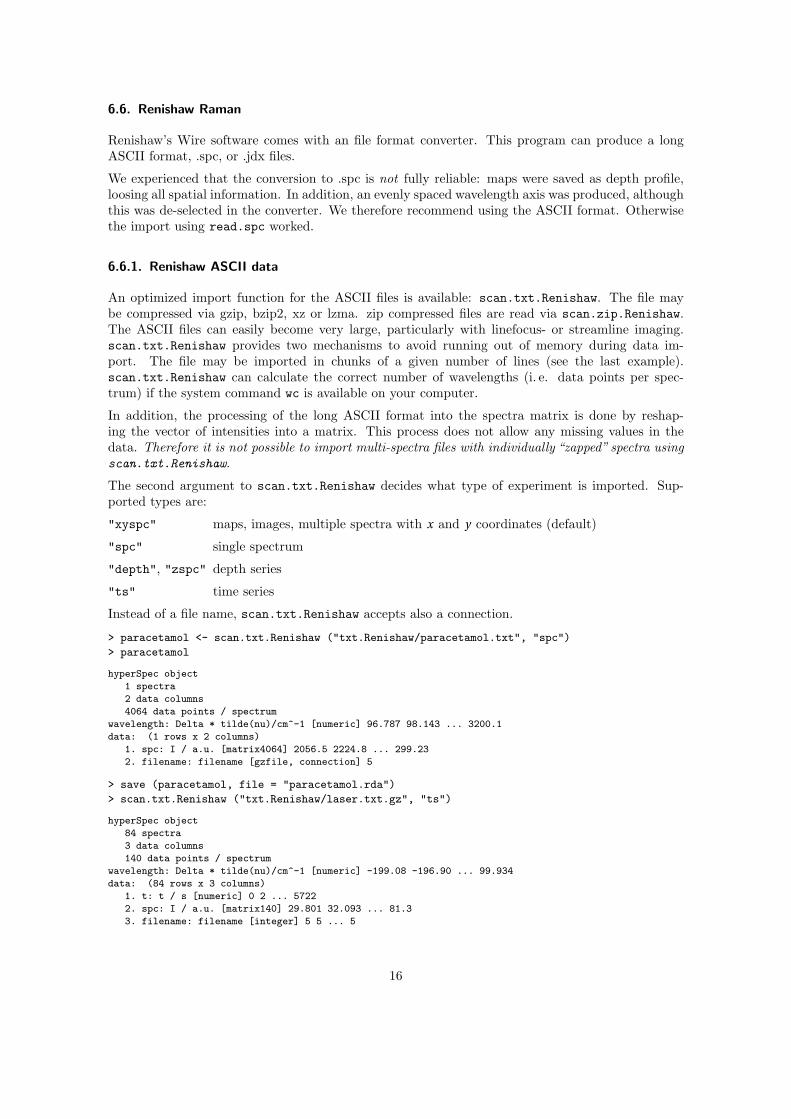
6.6. Renishaw Raman

Renishaw’s Wire software comes with an file format converter. This program can produce a longASCII format, .spc, or .jdx files.

We experienced that the conversion to .spc is not fully reliable: maps were saved as depth profile,loosing all spatial information. In addition, an evenly spaced wavelength axis was produced, althoughthis was de-selected in the converter. We therefore recommend using the ASCII format. Otherwisethe import using read.spc worked.

6.6.1. Renishaw ASCII data

An optimized import function for the ASCII files is available: scan.txt.Renishaw. The file maybe compressed via gzip, bzip2, xz or lzma. zip compressed files are read via scan.zip.Renishaw.The ASCII files can easily become very large, particularly with linefocus- or streamline imaging.scan.txt.Renishaw provides two mechanisms to avoid running out of memory during data im-port. The file may be imported in chunks of a given number of lines (see the last example).scan.txt.Renishaw can calculate the correct number of wavelengths (i. e. data points per spec-trum) if the system command wc is available on your computer.

In addition, the processing of the long ASCII format into the spectra matrix is done by reshap-ing the vector of intensities into a matrix. This process does not allow any missing values in thedata. Therefore it is not possible to import multi-spectra files with individually “zapped” spectra usingscan.txt.Renishaw.

The second argument to scan.txt.Renishaw decides what type of experiment is imported. Sup-ported types are:

"xyspc" maps, images, multiple spectra with x and y coordinates (default)

"spc" single spectrum

"depth", "zspc" depth series

"ts" time series

Instead of a file name, scan.txt.Renishaw accepts also a connection.

> paracetamol <- scan.txt.Renishaw ("txt.Renishaw/paracetamol.txt", "spc")

> paracetamol

hyperSpec object

1 spectra

2 data columns


wavelength: Delta * tilde(nu)/cm^-1 [numeric] 96.787 98.143 ... 3200.1


1. spc: I / a.u. [matrix4064] 2056.5 2224.8 ... 299.23

2. filename: filename [gzfile, connection] 5

> save (paracetamol, file = "paracetamol.rda")

> scan.txt.Renishaw ("txt.Renishaw/laser.txt.gz", "ts")

hyperSpec object

84 spectra

3 data columns


wavelength: Delta * tilde(nu)/cm^-1 [numeric] -199.08 -196.90 ... 99.934


1. t: t / s [numeric] 0 2 ... 5722

2. spc: I / a.u. [matrix140] 29.801 32.093 ... 81.3

3. filename: filename [integer] 5 5 ... 5

16

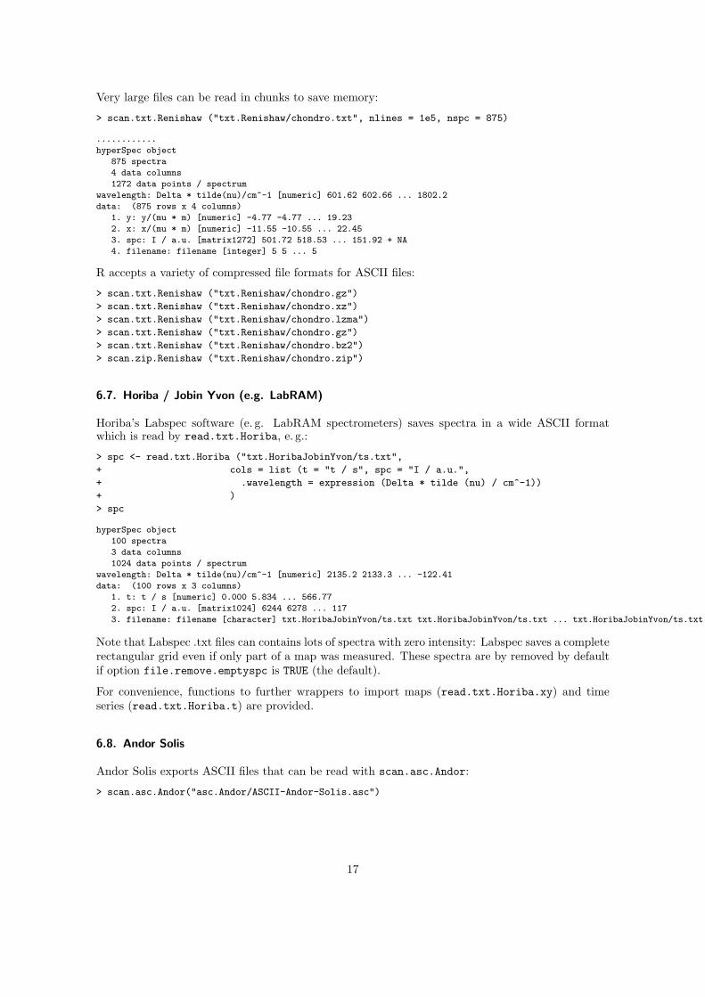
Very large files can be read in chunks to save memory:

> scan.txt.Renishaw ("txt.Renishaw/chondro.txt", nlines = 1e5, nspc = 875)

............

hyperSpec object

875 spectra

4 data columns


wavelength: Delta * tilde(nu)/cm^-1 [numeric] 601.62 602.66 ... 1802.2


1. y: y/(mu * m) [numeric] -4.77 -4.77 ... 19.23

2. x: x/(mu * m) [numeric] -11.55 -10.55 ... 22.45

3. spc: I / a.u. [matrix1272] 501.72 518.53 ... 151.92 + NA

4. filename: filename [integer] 5 5 ... 5

R accepts a variety of compressed file formats for ASCII files:

> scan.txt.Renishaw ("txt.Renishaw/chondro.gz")

> scan.txt.Renishaw ("txt.Renishaw/chondro.xz")

> scan.txt.Renishaw ("txt.Renishaw/chondro.lzma")

> scan.txt.Renishaw ("txt.Renishaw/chondro.gz")

> scan.txt.Renishaw ("txt.Renishaw/chondro.bz2")

> scan.zip.Renishaw ("txt.Renishaw/chondro.zip")

6.7. Horiba / Jobin Yvon (e.g. LabRAM)

Horiba’s Labspec software (e. g. LabRAM spectrometers) saves spectra in a wide ASCII formatwhich is read by read.txt.Horiba, e. g.:

> spc <- read.txt.Horiba ("txt.HoribaJobinYvon/ts.txt",

+ cols = list (t = "t / s", spc = "I / a.u.",

+ .wavelength = expression (Delta * tilde (nu) / cm^-1))

+ )

> spc

hyperSpec object

100 spectra

3 data columns


wavelength: Delta * tilde(nu)/cm^-1 [numeric] 2135.2 2133.3 ... -122.41


1. t: t / s [numeric] 0.000 5.834 ... 566.77

2. spc: I / a.u. [matrix1024] 6244 6278 ... 117

3. filename: filename [character] txt.HoribaJobinYvon/ts.txt txt.HoribaJobinYvon/ts.txt ... txt.HoribaJobinYvon/ts.txt

Note that Labspec .txt files can contains lots of spectra with zero intensity: Labspec saves a completerectangular grid even if only part of a map was measured. These spectra are by removed by defaultif option file.remove.emptyspc is TRUE (the default).

For convenience, functions to further wrappers to import maps (read.txt.Horiba.xy) and timeseries (read.txt.Horiba.t) are provided.

6.8. Andor Solis

Andor Solis exports ASCII files that can be read with scan.asc.Andor:

> scan.asc.Andor("asc.Andor/ASCII-Andor-Solis.asc")

17

hyperSpec object

5 spectra

2 data columns




1. spc: [matrix63] 3404 3402 ... 3415

2. filename: filename [character] asc.Andor/ASCII-Andor-Solis.asc asc.Andor/ASCII-Andor-Solis.asc asc.Andor/ASCII-Andor-

6.9. Witec

The Witec project software supports exporting spectra as Thermo Galactic .spc files.

> read.spc ("spc.Witec/Witec-timeseries.spc")

> read.spc ("spc.Witec/Witec-Map.spc")

.spc is in general the recommended format for hyperSpec import. For imaging data no spatialinformation for the set of spectra is provided (in version 2.10 this export option is not supported).

Imaging data (but also single spectra and time series) can be exported as ASCII X and Y files (SaveASCII X and Save ASCII Y, not supported in version 4). These can be read by scan.dat.Witec:

> scan.dat.Witec ("txt.Witec/Witec-timeseries-x.dat")

> scan.dat.Witec (filex = "txt.Witec/Witec-Map-x.dat",

+ points.per.line = 5, lines.per.image = 5, type = "map")

Note that the Y data files also contain a wavelength information, but (at least Witec Project 2.10)this information is always wavelength in nm, not Raman shift in wavenumbers: this is provided bythe X data file only.

Another option is Witec’s txt table ASCII export (Export → Table), which produces ASCII fileswith each row corresponding to one wavelength. The first column contains the wavelength axis, allfurther columns contain one spectrum each column. Such files can be read with scan.txt.Witec:

> scan.txt.Witec ("txt.Witec/Witec-timeseries_no.txt")

scan.txt.Witec determines the number of wavelengths automaticallly.

Note that there are several Export Filter Options. Here you can determine, which units should beused for the export (see XUnits tab). In addition, it is possible to export two additional header linescontaining information about spectra labels and units. Therefore parameters hdr.label and hdr.unitshave to be set properly. Otherwise, either an error will be displayed like

Error in scan(file, what, nmax, sep, dec, quote, skip, nlines, na.strings, :

scan() expected 'a real', got 'rel.'

or the one or two wavelengths will be skipped.

Depending on the used export options the header files should look like:

with exported labels and units headerlines:

X-Axis Time Series_000_Spec.Data 1(0) Time Series_000_Spec.Data 1(1)

rel. 1/cm CCD cts CCD cts

8.77367E+01 9.95000E+02 9.94000E+02

9.10310E+01 9.96000E+02 9.94000E+02

with exported labels headerline:

X-Axis Time Series_000_Spec.Data 1(0) Time Series_000_Spec.Data 1(1)

8.77367E+01 9.95000E+02 9.94000E+02

9.10310E+01 9.96000E+02 9.94000E+02

9.43239E+01 9.92000E+02 9.92000E+02

with exported units headerline:

rel. 1/cm CCD cts CCD cts

18

8.77367E+01 9.95000E+02 9.94000E+02

9.10310E+01 9.96000E+02 9.94000E+02

9.43239E+01 9.92000E+02 9.92000E+02

without headerline:

87.737 995.000 994.000

91.031 996.000 994.000

94.324 992.000 992.000

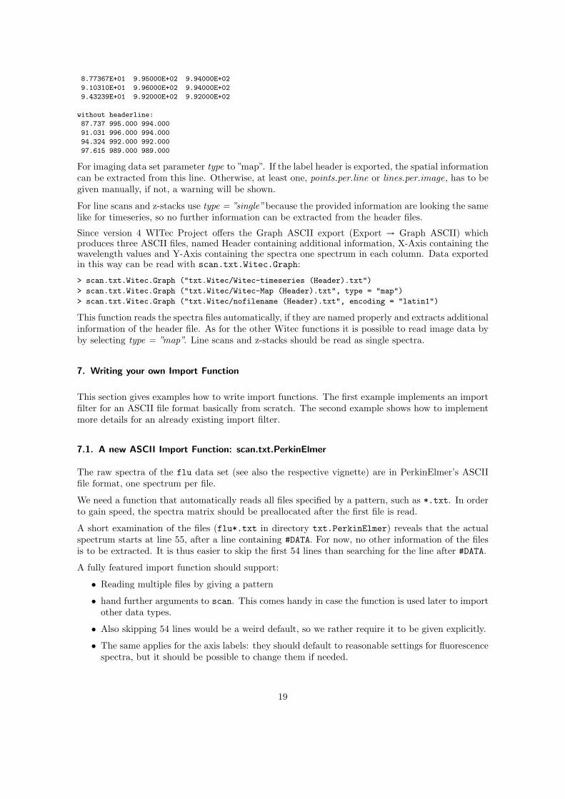
97.615 989.000 989.000

For imaging data set parameter type to ”map”. If the label header is exported, the spatial informationcan be extracted from this line. Otherwise, at least one, points.per.line or lines.per.image, has to begiven manually, if not, a warning will be shown.

For line scans and z-stacks use type = ”single”because the provided information are looking the samelike for timeseries, so no further information can be extracted from the header files.

Since version 4 WITec Project offers the Graph ASCII export (Export → Graph ASCII) whichproduces three ASCII files, named Header containing additional information, X-Axis containing thewavelength values and Y-Axis containing the spectra one spectrum in each column. Data exportedin this way can be read with scan.txt.Witec.Graph:

> scan.txt.Witec.Graph ("txt.Witec/Witec-timeseries (Header).txt")

> scan.txt.Witec.Graph ("txt.Witec/Witec-Map (Header).txt", type = "map")

> scan.txt.Witec.Graph ("txt.Witec/nofilename (Header).txt", encoding = "latin1")

This function reads the spectra files automatically, if they are named properly and extracts additionalinformation of the header file. As for the other Witec functions it is possible to read image data byby selecting type = ”map”. Line scans and z-stacks should be read as single spectra.

7. Writing your own Import Function

This section gives examples how to write import functions. The first example implements an importfilter for an ASCII file format basically from scratch. The second example shows how to implementmore details for an already existing import filter.

7.1. A new ASCII Import Function: scan.txt.PerkinElmer

The raw spectra of the flu data set (see also the respective vignette) are in PerkinElmer’s ASCIIfile format, one spectrum per file.

We need a function that automatically reads all files specified by a pattern, such as *.txt. In orderto gain speed, the spectra matrix should be preallocated after the first file is read.

A short examination of the files (flu*.txt in directory txt.PerkinElmer) reveals that the actualspectrum starts at line 55, after a line containing #DATA. For now, no other information of the filesis to be extracted. It is thus easier to skip the first 54 lines than searching for the line after #DATA.

A fully featured import function should support:

• Reading multiple files by giving a pattern

• hand further arguments to scan. This comes handy in case the function is used later to importother data types.

• Also skipping 54 lines would be a weird default, so we rather require it to be given explicitly.

• The same applies for the axis labels: they should default to reasonable settings for fluorescencespectra, but it should be possible to change them if needed.

19

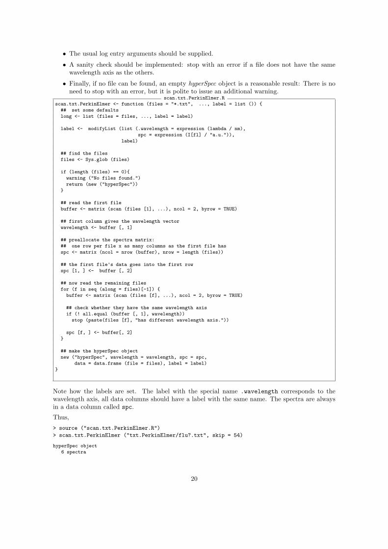
• The usual log entry arguments should be supplied.

• A sanity check should be implemented: stop with an error if a file does not have the samewavelength axis as the others.

• Finally, if no file can be found, an empty hyperSpec object is a reasonable result: There is noneed to stop with an error, but it is polite to issue an additional warning.

scan.txt.PerkinElmer.Rscan.txt.PerkinElmer <- function (files = "*.txt", ..., label = list ()) {

## set some defaults

long <- list (files = files, ..., label = label)

label <- modifyList (list (.wavelength = expression (lambda / nm),

spc = expression (I[fl] / "a.u.")),

label)

## find the files

files <- Sys.glob (files)

if (length (files) == 0){

warning ("No files found.")

return (new ("hyperSpec"))

}

## read the first file

buffer <- matrix (scan (files [1], ...), ncol = 2, byrow = TRUE)

## first column gives the wavelength vector

wavelength <- buffer [, 1]

## preallocate the spectra matrix:

## one row per file x as many columns as the first file has

spc <- matrix (ncol = nrow (buffer), nrow = length (files))

## the first file's data goes into the first row

spc [1, ] <- buffer [, 2]

## now read the remaining files

for (f in seq (along = files)[-1]) {

buffer <- matrix (scan (files [f], ...), ncol = 2, byrow = TRUE)

## check whether they have the same wavelength axis

if (! all.equal (buffer [, 1], wavelength))

stop (paste(files [f], "has different wavelength axis."))

spc [f, ] <- buffer[, 2]

}

## make the hyperSpec object

new ("hyperSpec", wavelength = wavelength, spc = spc,

data = data.frame (file = files), label = label)

}

Note how the labels are set. The label with the special name .wavelength corresponds to thewavelength axis, all data columns should have a label with the same name. The spectra are alwaysin a data column called spc.

Thus,

> source ("scan.txt.PerkinElmer.R")

> scan.txt.PerkinElmer ("txt.PerkinElmer/flu?.txt", skip = 54)

hyperSpec object

6 spectra

20

2 data columns


wavelength: lambda/nm [numeric] 405.0 405.5 ... 495


1. file: [factor] txt.PerkinElmer/flu1.txt txt.PerkinElmer/flu2.txt ... txt.PerkinElmer/flu6.txt

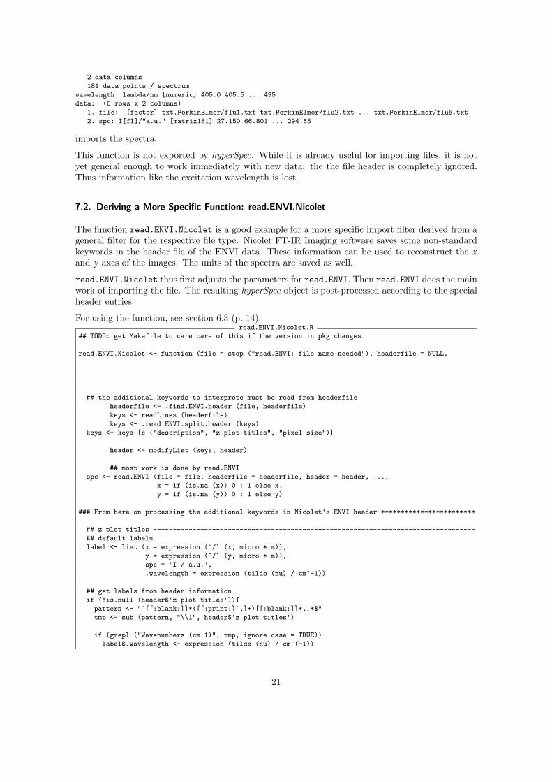
2. spc: I[fl]/"a.u." [matrix181] 27.150 66.801 ... 294.65

imports the spectra.

This function is not exported by hyperSpec. While it is already useful for importing files, it is notyet general enough to work immediately with new data: the the file header is completely ignored.Thus information like the excitation wavelength is lost.

7.2. Deriving a More Specific Function: read.ENVI.Nicolet

The function read.ENVI.Nicolet is a good example for a more specific import filter derived from ageneral filter for the respective file type. Nicolet FT-IR Imaging software saves some non-standardkeywords in the header file of the ENVI data. These information can be used to reconstruct the x

and y axes of the images. The units of the spectra are saved as well.

read.ENVI.Nicolet thus first adjusts the parameters for read.ENVI. Then read.ENVI does the mainwork of importing the file. The resulting hyperSpec object is post-processed according to the specialheader entries.

For using the function, see section 6.3 (p. 14).read.ENVI.Nicolet.R

## TODO: get Makefile to care care of this if the version in pkg changes

read.ENVI.Nicolet <- function (file = stop ("read.ENVI: file name needed"), headerfile = NULL,

## the additional keywords to interprete must be read from headerfile

headerfile <- .find.ENVI.header (file, headerfile)

keys <- readLines (headerfile)

keys <- .read.ENVI.split.header (keys)

keys <- keys [c ("description", "z plot titles", "pixel size")]

header <- modifyList (keys, header)

## most work is done by read.ENVI

spc <- read.ENVI (file = file, headerfile = headerfile, header = header, ...,

x = if (is.na (x)) 0 : 1 else x,

y = if (is.na (y)) 0 : 1 else y)

### From here on processing the additional keywords in Nicolet's ENVI header ************************

## z plot titles ----------------------------------------------------------------------------------

## default labels

label <- list (x = expression (`/` (x, micro * m)),

y = expression (`/` (y, micro * m)),

spc = 'I / a.u.',

.wavelength = expression (tilde (nu) / cm^-1))

## get labels from header information

if (!is.null (header$'z plot titles')){

pattern <- "^[[:blank:]]*([[:print:]^,]+)[[:blank:]]*,.*$"

tmp <- sub (pattern, "\\1", header$'z plot titles')

if (grepl ("Wavenumbers (cm-1)", tmp, ignore.case = TRUE))

label$.wavelength <- expression (tilde (nu) / cm^(-1))

21

else

label$.wavelength <- tmp

pattern <- "^[[:blank:]]*[[:print:]^,]+,[[:blank:]]*([[:print:]^,]+).*$"

tmp <- sub (pattern, "\\1", header$'z plot titles')

if (grepl ("Unknown", tmp, ignore.case = TRUE))

label$spc <- "I / a.u."

else

label$spc <- tmp

}

## modify the labels accordingly

spc@label <- modifyList (label, spc@label)

## set up spatial coordinates ---------------------------------------------------------------------

## look for x and y in the header only if x and y are NULL

## they are in `description` and `pixel size`

## set up regular expressions to extract the values

p.description <- paste ("^Spectrum position [[:digit:]]+ of [[:digit:]]+ positions,",

"X = ([[:digit:].-]+), Y = ([[:digit:].-]+)$")

p.pixel.size <- "^[[:blank:]]*([[:digit:].-]+),[[:blank:]]*([[:digit:].-]+).*$"

if (is.na (x) && is.na (y) &&

! is.null (header$description) && grepl (p.description, header$description ) &&

! is.null (header$'pixel size') && grepl (p.pixel.size, header$'pixel size')) {

x [1] <- as.numeric (sub (p.description, "\\1", header$description))

y [1] <- as.numeric (sub (p.description, "\\2", header$description))

x [2] <- as.numeric (sub (p.pixel.size, "\\1", header$'pixel size'))

y [2] <- as.numeric (sub (p.pixel.size, "\\2", header$'pixel size'))

## it seems that the step size is given in mm while the offset is in micron

if (nicolet.correction) {

x [2] <- x [2] * 1000

y [2] <- y [2] * 1000

}

## now calculate and set the x and y coordinates

x <- x [2] * spc$x + x [1]

if (! any (is.na (x)))

spc@data$x <- x

y <- y [2] * spc$y + y [1]

if (! any (is.na (y)))

spc@data$y <- y

}

spc

}

7.3. Deriving import filters for spc files

Please note that future changes inside the read.spc function are likely to occur. However, if you justpost-process the hyperSpec object returned by read.spc, you should be fine.

References

[1] Robert S. McDonald and Jr. Paul A. Wilks. Jcamp-dx: A standard form for the exchange ofinfrared spectra in computer readable form. Applied Spectroscopy, 42(1):151–162, 1988.

22

[2] Henrik Bengtsson. R.matlab: Read and Write MAT Files and Call MATLAB from Within R,2016. URL https://CRAN.R-project.org/package=R.matlab. R package version 3.6.1.

[3] Universal Data Format Specification. Galactic Industries Corp., 1997. URL http://ftirsearch.

com/features/converters/gspc_udf.zip.

23

https://CRAN.R-project.org/package=R.matlab

http://ftirsearch.com/features/converters/gspc_udf.zip

http://ftirsearch.com/features/converters/gspc_udf.zip

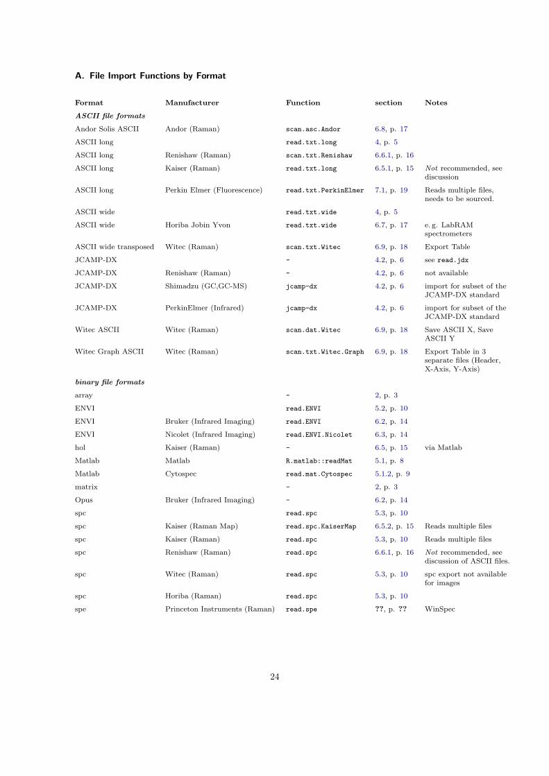
A. File Import Functions by Format

Format Manufacturer Function section Notes

ASCII file formats

Andor Solis ASCII Andor (Raman) scan.asc.Andor 6.8, p. 17

ASCII long read.txt.long 4, p. 5

ASCII long Renishaw (Raman) scan.txt.Renishaw 6.6.1, p. 16

ASCII long Kaiser (Raman) read.txt.long 6.5.1, p. 15 Not recommended, seediscussion

ASCII long Perkin Elmer (Fluorescence) read.txt.PerkinElmer 7.1, p. 19 Reads multiple files,needs to be sourced.

ASCII wide read.txt.wide 4, p. 5

ASCII wide Horiba Jobin Yvon read.txt.wide 6.7, p. 17 e. g. LabRAMspectrometers

ASCII wide transposed Witec (Raman) scan.txt.Witec 6.9, p. 18 Export Table

JCAMP-DX - 4.2, p. 6 see read.jdx

JCAMP-DX Renishaw (Raman) - 4.2, p. 6 not available

JCAMP-DX Shimadzu (GC,GC-MS) jcamp-dx 4.2, p. 6 import for subset of theJCAMP-DX standard

JCAMP-DX PerkinElmer (Infrared) jcamp-dx 4.2, p. 6 import for subset of theJCAMP-DX standard

Witec ASCII Witec (Raman) scan.dat.Witec 6.9, p. 18 Save ASCII X, SaveASCII Y

Witec Graph ASCII Witec (Raman) scan.txt.Witec.Graph 6.9, p. 18 Export Table in 3separate files (Header,X-Axis, Y-Axis)

binary file formats

array - 2, p. 3

ENVI read.ENVI 5.2, p. 10

ENVI Bruker (Infrared Imaging) read.ENVI 6.2, p. 14

ENVI Nicolet (Infrared Imaging) read.ENVI.Nicolet 6.3, p. 14

hol Kaiser (Raman) - 6.5, p. 15 via Matlab

Matlab Matlab R.matlab::readMat 5.1, p. 8

Matlab Cytospec read.mat.Cytospec 5.1.2, p. 9

matrix - 2, p. 3

Opus Bruker (Infrared Imaging) - 6.2, p. 14

spc read.spc 5.3, p. 10

spc Kaiser (Raman Map) read.spc.KaiserMap 6.5.2, p. 15 Reads multiple files

spc Kaiser (Raman) read.spc 5.3, p. 10 Reads multiple files

spc Renishaw (Raman) read.spc 6.6.1, p. 16 Not recommended, seediscussion of ASCII files.

spc Witec (Raman) read.spc 5.3, p. 10 spc export not availablefor images

spc Horiba (Raman) read.spc 5.3, p. 10

spe Princeton Instruments (Raman) read.spe ??, p. ?? WinSpec

24

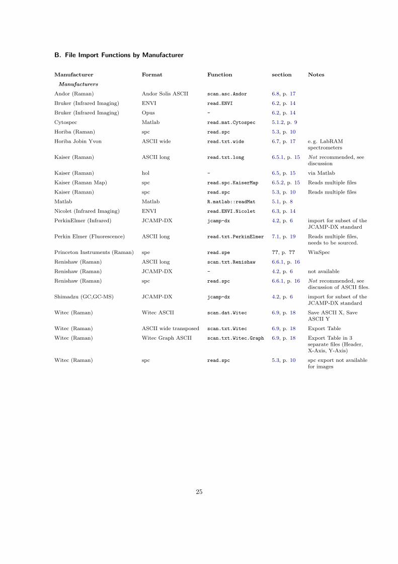
B. File Import Functions by Manufacturer

Manufacturer Format Function section Notes

Manufacturers

Andor (Raman) Andor Solis ASCII scan.asc.Andor 6.8, p. 17

Bruker (Infrared Imaging) ENVI read.ENVI 6.2, p. 14

Bruker (Infrared Imaging) Opus - 6.2, p. 14

Cytospec Matlab read.mat.Cytospec 5.1.2, p. 9

Horiba (Raman) spc read.spc 5.3, p. 10

Horiba Jobin Yvon ASCII wide read.txt.wide 6.7, p. 17 e. g. LabRAMspectrometers

Kaiser (Raman) ASCII long read.txt.long 6.5.1, p. 15 Not recommended, seediscussion

Kaiser (Raman) hol - 6.5, p. 15 via Matlab

Kaiser (Raman Map) spc read.spc.KaiserMap 6.5.2, p. 15 Reads multiple files

Kaiser (Raman) spc read.spc 5.3, p. 10 Reads multiple files

Matlab Matlab R.matlab::readMat 5.1, p. 8

Nicolet (Infrared Imaging) ENVI read.ENVI.Nicolet 6.3, p. 14

PerkinElmer (Infrared) JCAMP-DX jcamp-dx 4.2, p. 6 import for subset of theJCAMP-DX standard

Perkin Elmer (Fluorescence) ASCII long read.txt.PerkinElmer 7.1, p. 19 Reads multiple files,needs to be sourced.

Princeton Instruments (Raman) spe read.spe ??, p. ?? WinSpec

Renishaw (Raman) ASCII long scan.txt.Renishaw 6.6.1, p. 16

Renishaw (Raman) JCAMP-DX - 4.2, p. 6 not available

Renishaw (Raman) spc read.spc 6.6.1, p. 16 Not recommended, seediscussion of ASCII files.

Shimadzu (GC,GC-MS) JCAMP-DX jcamp-dx 4.2, p. 6 import for subset of theJCAMP-DX standard

Witec (Raman) Witec ASCII scan.dat.Witec 6.9, p. 18 Save ASCII X, SaveASCII Y

Witec (Raman) ASCII wide transposed scan.txt.Witec 6.9, p. 18 Export Table

Witec (Raman) Witec Graph ASCII scan.txt.Witec.Graph 6.9, p. 18 Export Table in 3separate files (Header,X-Axis, Y-Axis)

Witec (Raman) spc read.spc 5.3, p. 10 spc export not availablefor images

25

C. File Import Functions by Spectroscopy

Spectroscopy Format Manufacturer Function section Notes

Fluorescence ASCII long Perkin Elmer read.txt.PerkinElmer 7.1, p. 19 Reads multiple files,needs to be sourced.

GC,GC-MS JCAMP-DX Shimadzu jcamp-dx 4.2, p. 6 import for subset ofthe JCAMP-DXstandard

Infrared JCAMP-DX PerkinElmer jcamp-dx 4.2, p. 6 import for subset ofthe JCAMP-DXstandard

Infrared Imaging ENVI Bruker read.ENVI 6.2, p. 14

Infrared Imaging ENVI Nicolet read.ENVI.Nicolet 6.3, p. 14

Infrared Imaging Opus Bruker - 6.2, p. 14

Raman Andor Solis ASCII Andor scan.asc.Andor 6.8, p. 17

Raman ASCII long Renishaw scan.txt.Renishaw 6.6.1, p. 16

Raman ASCII long Kaiser read.txt.long 6.5.1, p. 15 Not recommended,see discussion

Raman ASCII wide transposed Witec scan.txt.Witec 6.9, p. 18 Export Table

Raman hol Kaiser - 6.5, p. 15 via Matlab

Raman JCAMP-DX Renishaw - 4.2, p. 6 not available

Raman spc Kaiser read.spc 5.3, p. 10 Reads multiple files

Raman spc Renishaw read.spc 6.6.1, p. 16 Not recommended,see discussion ofASCII files.

Raman spc Witec read.spc 5.3, p. 10 spc export notavailable for images

Raman spc Horiba read.spc 5.3, p. 10

Raman spe Princeton Instruments read.spe ??, p. ?? WinSpec

Raman Witec ASCII Witec scan.dat.Witec 6.9, p. 18 Save ASCII X, SaveASCII Y

Raman Witec Graph ASCII Witec scan.txt.Witec.Graph 6.9, p. 18 Export Table in 3separate files(Header, X-Axis,Y-Axis)

Raman Map spc Kaiser read.spc.KaiserMap 6.5.2, p. 15 Reads multiple files

D. Unit Test Results

DONE ===============================================================================================

26

Index

AgilentENVI, 14

Andor SolisASCII, 17

ASCIIAndor Solis, 17compressed, 16JCAMP-DX, 6long, 5

Fluorescence, 19Kaiser, 15PerkinElmer, 19Raman, 15, 16Renishaw, 16

samples in columns, 5transposed, 5wide, 5

Horiba, 17Horiba Jobin Yvon, 17LabRAM, see Horiba

Witec, 18zip, 16

atomic emissionNIST, 7

BrukerAXS, 5ENVI, 10, 14powder diffraction, 5x-ray, 5

create hyperSpec object, 3Cytospec, 9

Matlab, 9

ENVIAgilent, 14Bruker, 10, 14Infrared, 10, 14

Nicolet, 21Map, 10, 14, 21Nicolet, 14, 21Varian, 10

FluorescenceASCII long, 19PerkinElmer

ASCII, 19FT-IR, see Infrared

Graph ASCIIWitec, 18

holKaiser, 15

HoribaASCII

wide, 17spc, 10

Horiba Jobin YvonASCII

wide, 17

hyperSpec objectcreate, 3

Image, see MapInfrared

ENVI, 10, 14, 21JCAMP-DX, 6Map, 21Nicolet, 21PerkinElmer, 6

initialize hyperSpec object, 3

JCAMP-DXASCII, 6Infrared, 6PerkinElmer, 6Shimadzu, 6

jdx, see JCAMP-DX

KaiserASCII long, 15hol, 15Map, 15spc, 10, 15

LabRAM, see HoribaLabRam

spc, 10LabSpec

spc, 10

Map, 15ENVI, 10, 14Kaiser, 15Raman, 15

Matlab, 8Cytospec, 9

new hyperSpec object, 3Nicolet

ENVI, 14, 21Infrared, 21Map, 21

NISTatomic emission, 7

PerkinElmerASCII long, 19Fluorescence, 19Infrared, 6JCAMP-DX, 6

powder diffractionBruker, 5

RamanAndor Solis

ASCII, 17ASCII long, 15, 16hol, 15HoloGram, 10Horiba, 10

ASCII wide, 17

27

Horiba Jobin YvonASCII wide, 17

Kaiser, 10, 15LabRAM, see HoribaLabRam, 10LabSpec, 10Map, 15Renishaw, 10

ASCII, 16spc, 16

spc, 10, 15Witec

ASCII, 18Export Table, 18Graph ASCII, 18Save ASCII X, Save ASCII Y, 18spc, 18

referenceNIST

atomic emission, 7Renishaw

ASCII long, 16Raman, 16spc, 10, 16

ShimadzuGC-MS, 6JCAMP-DX, 6

spc, 10Kaiser, 10, 15Raman, 10, 15, 16Renishaw, 10, 16TriVista, 10Witec, 18

TriVistaspc, 10

Varian, see AgilentENVI, 10

WitecASCII, 18Graph ASCII, 18

x-rayBruker, 5

28

Session Info

R version 3.2.3 (2015-12-10)

Platform: x86_64-pc-linux-gnu (64-bit)

Running under: Ubuntu 16.04.2 LTS

locale:

[1] LC_CTYPE=de_DE.UTF-8 LC_NUMERIC=C LC_TIME=de_DE.UTF-8

[4] LC_COLLATE=de_DE.UTF-8 LC_MONETARY=de_DE.UTF-8 LC_MESSAGES=de_DE.UTF-8

[7] LC_PAPER=de_DE.UTF-8 LC_NAME=C LC_ADDRESS=C

[10] LC_TELEPHONE=C LC_MEASUREMENT=de_DE.UTF-8 LC_IDENTIFICATION=C

attached base packages:

[1] grid stats graphics grDevices utils datasets methods base

other attached packages:

[1] digest_0.6.12 testthat_1.0.2 hyperSpec_0.98-20170630 ggplot2_2.2.1

[5] lattice_0.20-35

loaded via a namespace (and not attached):

[1] Rcpp_0.12.11 crayon_1.3.2 R.methodsS3_1.7.1 R.matlab_3.6.1

[5] plyr_1.8.4 R6_2.2.2 gtable_0.2.0 magrittr_1.5

[9] scales_0.4.1 rlang_0.1.1 lazyeval_0.2.0 R.utils_2.5.0

[13] R.oo_1.21.0 latticeExtra_0.6-28 RColorBrewer_1.1-2 tools_3.2.3

[17] munsell_0.4.3 colorspace_1.3-2 tibble_1.3.3

29

Documents

Import and Export of Spectra Files - The · PDF fileImport and Export of Spectra Files ... please send an email to ... labels a list with the proper labels