Implicit Large Eddy Simulationof a wingtip vortexat Rec = 1.2 · 106

Jean-Eloi W. Lombard∗, David Moxey†, Julien F. A. Hoessler‡,Sridar Dhandapani§, Mark J. Taylor¶, Spencer J. Sherwin‖

Abstract

In this article we present recent developments in numerical methods for performing a Large EddySimulation (LES) of the formation and evolution of a wingtip vortex. The development of these vortices inthe near wake, in combination with the large Reynolds numbers present in these cases, make these typesof test cases particularly challenging to investigate numerically. We first give an overview of the SpectralVanishing Viscosity–implicit LES (SVV-iLES) solver that is used to perform the simulations, and highlighttechniques that have been adopted to solve various numerical issues that arise when studying such cases.To demonstrate the method’s viability, we present results from numerical simulations of flow over a NACA0012 profile wingtip at Rec = 1.2 · 106 and compare them against experimental data, which is to date thehighest Reynolds number achieved for a LES that has been correlated with experiments for this test case.Our model correlates favorably with experiment, both for the characteristic jetting in the primary vortexand pressure distribution on the wing surface. The proposed method is of general interest for the modelingof transitioning vortex dominated flows over complex geometries.

Nomenclaturec = Wing chordb = wingspanA = aspect ratio of the wingRec = Reynolds number based on wing chordx,y,z = Carterisan coordinates,∆x = local cell sizeu,v,w = Cartesian velocity componentsy+ = distance from surface in wall unitst = timetc = convective time associate to chord∆t = time-stepl0 = length scale associate to largest eddiesη = Kolmogorov length scale

τ = Kolmogorov time scalep = pressurep = far-field pressureU∞ = inflow velocityρ∞ = densityCp = Pressure coefficientν = kinematic viscosityα = angle of attackk = modeM = cut-off mode of the SVV filterP = P = M − 1 polynomial order of the spectral element.εSV V = diffusion from the SVV filterQ = SVV kernel

1 IntroductionUnderstanding the development and growth of wingtip vortices over lifting surfaces is an ongoing research topicboth in academia and industry. From an academic perspective, fundamental open questions remain, such as∗Graduate Research Assistant, Department of Aeronautics, Imperial College, London, UK;

jean-eloi.lombard12@imperial.ac.uk (Corresponding Author).†Research Associate, Aeronautics, Department of Aeronautics, Imperial College, London, UK‡Senior CFD Engineer, CFD Technology, McLaren Racing, McLaren Technology Center, Woking, UK§Team Leader, CFD Technology, McLaren Racing, McLaren Technology Center, Woking, UK¶Principle Aerodynamicist, McLaren Racing, McLaren Technology Center, Woking, UK‖Professor of Computational Fluid Mechanics, Aeronautics.

1

arX

iv:1

507.

0601

2v1

[ph

ysic

s.fl

u-dy

n] 2

1 Ju

l 201

5

the possible re-laminarization of the vortex as it is shed from the wing [1] and the origin of meandering [2, 3, 4],the low-frequency movement of the vortex core and the evolution of the vortex structure. Vortices shed fromlifting surfaces pose challenges to model in many an industrial context such as wind turbines, helicopter blades,high-lift configuration of aircraft and high-performance automotive industry [5, 6, 7, 8, 9]. Developing a betterunderstanding of the near-wake of the vortex, lying within one chord length of the trailing edge of the liftingsurface, is therefore essential in understanding the complex flow-structure interactions of interest in theseproblems. The far-field properties of these vortices are also a challenge for the aeronautics industry, wheretheir persistence imposes strict limits on distances between landing aircraft [10]. For these reasons we areinterested in refining modeling methods for investigating the growth of the vortex in the near-field.

Conceptually, the simplest approach to ensure that the flow physics are accurately simulated is to performa direct numerical simulation (DNS), in which all necessary scales are resolved at a given Reynolds number.For cases at even moderately high Re however, this approach is clearly unfeasible. To demonstrate this, let usassume the Kolmogorov hypothesis holds for this flow and as a very rough approximation that the length scalel0 associated to the largest eddies is of the same order as the chord length l0 ≈ c. The number of grid pointsneeded to resolve the Kolmogorov length-scale relates with the Reynolds number as η ∼ Re−3/4 , meaningthat three-dimensional simulation of a uniformly turbulent flow requires a resolution of Re9/4 grid points. Foraeronautical test cases, where Re is typically O(106) or O(107), we therefore require O(1014) to O(1016) gridpoints to resolve the flow. Even accounting for variations in geometry which may permit varying resolutionthroughout the domain, based on the current rate of advancement of high-performance computing (HPC)facilities, resolving fully developed three-dimensional flow at high Reynolds number in a timely manner willcontinue to be well out of reach for the foreseeable future.

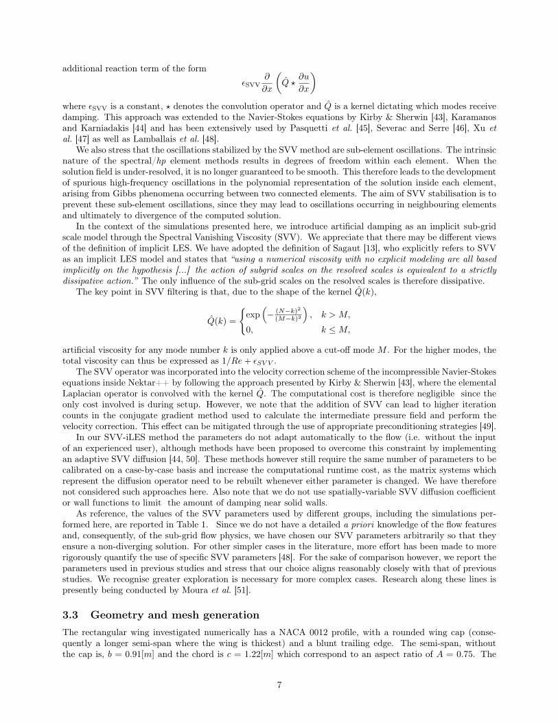
Figure 1: Wingtip vortex developing over a NACA 0012 profile with rounded wing cap in a wind tunnel,modeling the experimental setup of Chow et al.[1] Both wing surface and streamlines are colored by staticpressure coefficient Cp = 2 · (p− p∞)/ρ∞U

2∞ where U2

∞ = 1 and ρ∞ = 1.

Consequently, there has been ongoing development of modeling methods where small turbulent scales arenot explicitly computed. Traditional Reynolds Averaged Navier Stokes (RANS) methods, alongside morerecent advanced such as the Reynolds Stress methods [11], have been developed to simulate both the complexthree-dimensional transitioning boundary layer on the wing and the highly curved flow within the vortex. Morecomputationally-intensive methods, such as LES and Lattice Boltzman VLES[12] have also been developedor adapted to investigate such flows, in correlating the simulated results to experimental data. The latticeBoltzman method has been used in conjunction with a modified k − ε two-equation turbulence model as wellas turbulence wall shear stress model were used to perform a VLES where the walls were the turbulent flowat the wall was modelled.

The key feature of these studies is in their use of reduced equations or turbulence models, all of which requireparameters to tune their performance. Since the underlying physical processes that dictate the developmentand evolution of vortices is not well understood, it is therefore difficult a priori to determine appropriatesettings for these models. The aim of this work is therefore to demonstrate how an implicit LES method,in which the number of parameters is comparably very small and is used to provide additional stability, cansuccessfully be leveraged to obtain accurate comparisons against experimental data. We appreciate thatthere may be different views of the definition of implicit LES. We have adopted the definition of Sagaut [13],who explicitly refers to SVV as an implicit LES model and states that “using a numerical viscosity with no

2

explicit modeling are all based implicitly on the hypothesis [...] the action of subgrid scales on the resolvedscales is equivalent to a strictly dissipative action.” The only influence of the sub-grid scales on the resolvedscales is therefore dissipative.

Many existing LES codes are based on finite volume, linear finite element or Cartesian grid methods. Wewill instead investigate the viability of the spectral/hp element method, which lies in the class of high-orderfinite element methods. These methods are widely used in academia, as they offer attractive properties suchas exponential convergence and low dissipation error for sufficiently smooth solutions [14]. This is significant,as faithfully modeling the wingtip vortex in the far wake is of particular interest in many research communitiesand industries. It is implied that accurate modelling of the far field vortex requires precise modelling of thevortex onset in the near field using high precision, low dissipation schemes [15, 16, 1, 17, 18]. However, thesemethods have not been widely applied for the type of industrial, high-Re cases that we consider in this work.Such methods are generally perceived as difficult to implement, as a range of specialised preconditioners,mesh generation procedures, parallel communication strategies and stabilisation approaches are needed tosuccessfully complete a simulation.

In this paper we present the SVV-iLES formulation, which utilises the spectral vanishing viscosity approachto stabilise numerics [19]. We show how the issues of implementation and mesh generation can be overcome, aswell as highlight the benefits that these schemes can have for industrial problems, both in terms of resolutionpower relative to existing studies and computational efficiency. To demonstrate the viability and robustnessof the scheme, we consider the test case presented by Chow et al. [1], in which the flow over a NACA 0012wingtip has been investigated with precise experimental measurements. This case has subsequently become abenchmark for vortex dominated flows. To this end we perform an SVV-iLES, at the highest Reynolds numberconsidered so far for this case, and correlate our results to the experimental data. As in previous numericalstudies, in order to reduce the computational cost we have chosen to run the computation at a lower Reynoldsnumber. In this work we set Re = 1.2 · 106, as compared to the experiment which uses Re = 4.6 · 106.

In the following section we will briefly report the experimental and numerical methods that have beendeveloped and evaluated for investigating the nascent wingtip vortex, as well as the key findings of thesestudies. We then discuss the key features of the SVV-iLES method in Section 3 and the numerical methodologyfor our simulations. The evaluation of the SVV-iLES, by close comparison with the extensive data from theexperiment of Chow et al.[1] and numerical results of Uzun et al.[5], is presented in Section 4 before we concludein Section 5 with a brief overview of the key findings.

2 Literature reviewWe begin with a brief presentation of existing work in the investigation of wingtip vortices; other thoroughreviews of this field can be found in Rossow [7], Spalart [10] and Green & Acosta [20]. Firstly, experimentalstudies are considered and a summary of the types of flow dynamics that exists for these cases is presented.We then discuss results obtained by numerical simulations before emphasizing the possible drawbacks of anexplicit subgrid-scale model in the context of complex flows, such as the wingtip vortex and highlight theoriginality of the method employed in this study.

2.0.1 Experimental methods

For the wingtip vortex the Reynolds number is computed from the chord length c as Rec = cU∞/ν, whereU∞ is the free stream velocity and ν is the kinematic viscosity. Giuni [21, 22] and Giuni & Benard [23]investigated the initial formation and development of the wingtip vortex on a NACA 0012 rectangular wingwith both square and rounded wingtips at Rec = 7.4 · 105 for angles of attack α = 0, 4 and 12. Theyreported that for a given fixed angle of attack, a ‘more’ axisymmetric vortex sheds from the rounded wingtipwith stronger vorticity within its core compared the square-tip wing. They also reported that for the α = 12

case the axial velocity excess is higher for the rounded wingtip. This region is surrounded by a region ofaxial velocity deficit corresponding to rolling up of the vorticity sheet. The weaker axial velocity excess forthe square wingtip is believed to be a consequence of the more numerous secondary vortices generated by thesquare wingtip.

Defining the center of the primary vortex as the location of the streamwise helicity peak, they investigatedthe meandering of the vortex in the near field. Two distinct modes of behaviour were observed: for the

3

squared wingtip, the meandering decreased with the distance from the trailing edge whereas for the roundedwingtip case, the meandering grew quasi-linearly with distance from the trailing edge. This has also beenreported by Devenport et al. [2] and Giuni et al. [22]. However Jacquin et al. [3] concluded vortex meanderingto be insensitive to free stream unsteadiness in the wind tunnel. Fabre & Jacquin [24, 25] and Dieterle etal. [26] suggested meandering might also be influenced by the destabilization of a vortex by secondary vortexof opposite sense. Jacquin goes further by reporting that the various co-operative interactions between pri-mary and secondary vortices affected the same range of frequencies as meandering. Zuhal [27] and Zuhal &Gahrib [28] investigated the correlation between number and strength of secondary vortices and the amplitudeof meandering. McAlister [29] investigated the wingtip vortex of NACA 0015 with both rounded and squarewing cap reporting the maximum azimuthal velocity of the vortex to be independent of Reynolds number butdependent on the angle of attack.

Finally, Chow et al. [1] performed an extensive experimental and numerical study of the wingtip vortexover a rounded NACA 0012 profile in view of defining a benchmark for numerical models. They reportedmerging of the secondary and tertiary vortices into the primary within one chord length of the trailing edge.From this distance onwards, the vortex had an axisymmetric structure with a jet-like axial velocity profile(i.e. the axial velocity within the vortex core was greater than the freestream velocity). The peak jettingvelocity was measured to be 1.77U∞ at the trailing edge and by three-quarters of a chord length downstreamof the trailing edge it was measured to be 1.7U∞. Pressure taps were placed on the wing-surface to assess thestate of the boundary layer, both under the primary vortex where a strong suction region is present and atdifferent spanwise locations, allowing for insight into the three dimensional boundary layer. They also reportedskin-friction lines to gain understanding into the attachment and detachment lines of the strongest vortices inthe near wake, as well as low amplitudes of meandering because of both a relatively large angle of attack ofα = 10 and measurements at relatively short distances from the trailing edge. Devenport et al. [2] reportedmeandering amplitude growing linearly with distance from trailing edge.

2.0.2 Numerical methods

Presently, RANS based methods with linear eddy viscosity models, such as k − ω SST and k − ε, remaincommonplace for industrial flow simulation [11]. For vortex dominated flows, and more generally flows withstrong curvature, these models may struggle due to the largely unsteady dynamics of the flow. Large discrep-ancy with experimental data, exceeding 100% error on Cp distribution in the vortex core, as well as drasticunder-prediction of the jetting within the core have been reported by Churchfield et al. [30]. These resultshave motivated the development, over the past 30 years, of more complex closure models tailored for highlycurved flows such as the wingtip vortex. We present a brief overview of this development.

Dacles-Mariani et al. [9] ran a 5th order compact (i.e. 7 point stencil instead of 11) biased upwind schemefor the advection term and second order scheme for the viscous term. Here they underline the necessityfor low numerical dissipation. They ran a modified version of the one-equation Baldwin-Barth turbulencemodel where they modified the production term to avoid overproduction of eddy viscosity in the vortex core.They successfully captured a secondary structure and computed the axial velocity profiles of the core towithin 3% of experiment but under-predicted the core pressure by more than 25%. It should also be stressedthat Dacles-Mariani et al. [31] used experimental data to setup both inflow and outflow boundary conditionsfor their RANS simulation. Linear eddy-viscosity being too dissipative, Craft et al. [32] developed a non-linear eddy viscosity model (EVM). This more advanced model still suffered from a more severe decay of theturbulent stresses than measured experimentally. Duraisamy and Iaccarino [33] modified the eddy viscositycoefficient of the v2 − f turbulence model and compared their results favorably for axial surplus comparedto the baseline Spallart-Allmaras and Menter’s k − ω SST models. The wingtip vortex exhibits a peculiarityin the turbulence structures where the stress and strain are out of phase which renders questionable the useisotropic eddy-viscosity based prediction methods such as (k-ω, etc). Churchfield et al. [34, 35, 15, 11] modifiedthe Spalart-Allmaras model to account for streamline curvature and successfully modeled the lag between themean strain rate and respective Reynolds stress. This method produced the best correlation with experiment,for a RANS based method, but proved costly (relative to other simpler RANS methods) and so their use maybe restricted to flows dominated by vortices. They also showed that without the accurate modeling of thethree dimensional boundary layer the developing vortex remained challenging to compute accurately even forthe advanced RANS models correcting for the high degree of curvature in the flow.

In an attempt to develop increasingly robust models, more advanced numerical methods such as Large

4

Eddy Simulation (LES) and Very Large Eddy Simulations (VLES) have been proposed to investigate un-steady features of the flow as well as aero-acoustic properties. Fleigh et al. [36] developed a compressible LESto investigate far-field broadband noise generated by the nascent vortex on a rotating wingtip at ReynoldsRec = 1 · 106 and reported computed power and thrust coefficients for the windmill blade within 3% of ex-perimental data. Ghias [8] reported a compressible LES of NACA2415 with square tip run at Rec = 105

where they employed a dynamic sub-grid scale model but did not present the correlation of their data withexperiment. Uzun et al. [5, 6] numerically investigated Chow’s experiment with a compact finite differencingLES with implicit spatial filtering at Rec = 5 · 105. Their results were included in the following comparisonof our simulations with experimental data. Jiang et al. [37] reported results for a LES simulation of Chow’sexperiment at the experimental Reynolds number of Rec = 4.6 · 106 but did not compare the results withexperiment. The lattice Boltzman method was used in conjunction with a modified k−ε two equation turbu-lence model and wall shear stress model to perform a VLES. Despite good correlation with the experimentalresults of Chow et al. [1] for the suction of the vortex on the surface of the wing the method over-predicted thejetting phenomena within the vortex by 23% at streamwise location x/c = −0.114 and 12% at x/c = 0.456.So far these more advanced modeling methods have generally been used for simulations at lower Reynoldsnumbers [37, 6] or have not not been compared against experimental data in the way they will be in thepresent study [5].

2.0.3 Motivation and contributions of present study

Modeling unknown physics by leveraging a sub-grid scale model outside of its operational window can be seenas a substantial drawback for explicit sub-grid scale models, which tend to rely on a wide range of parametersto dictate their behaviour. The two-equation eddy-viscosity k − ω SST turbulence model introduced byMenter [38] in 1994, for example, relies on 9 modeling constants. Menter underlines, in this paper, the strongsensitivity of the resulting computed flow to variations of 5-10% of these constants and further stressing “Noneof the available theoretical tools (dimensional analysis, asymptotic expansion theory, use of direct numericalsimulations (DNS) data, renormalization group (RNG) theory, rapid distortion theory, etc.) can provideconstants to that degree of accuracy.” Leveraging these many parameter sub-grid scale models, such as k − ωSST and more recently Reynolds Stress Relaxation models [11], in complex flow cases therefore requires an apriori knowledge of the flow physics. This is often infeasible, particularly when complex geometries are presentand the length scales of both flow and geometry vary substantially. For example, in engineering applicationssuch as flow over a Formula 1 car, different sets of parameters may be required to accurately model the variousflow dynamics that are induced by the variations in geometry across the body of the the car. This includesthe vortex dominated flow of the wing-tip regions of a front wing, regions of the front wing where the flowis mostly two-dimensional, and the rotating wheel that impinges on the moving road. It may therefore beimpossible to obtain values for these parameters that capture the desired flow features across the entire car.

The aim of this paper is to show that regularized high order spectral/hp element methods, without anexplicit sub-grid model, can be applied to produce results that compare favorably against experimental data,by considering flow over a three-dimensional geometry of practical interest. The SVV-iLES approach, whichwe will present in the following section, requires the choice of two regularization parameters: one to dictate thelevel of artificial viscosity, and another for a cut-off wavenumber. These are chosen through experimentation,such that the computation does not diverge but do not require assumptions regarding the physics of the flow.We discuss this methodology in the following section before showing results of the NACA 0012 wingtip vortexcase.

3 Computational MethodologyIn this section, we give a brief summary of the computational methodology used for the NACA 0012 wingtipsimulations. We begin by outlining the Nektar++ spectral/hp element framework in which the solver isimplemented [39]. We then outline the types of regularization that are necessary to perform the computationsand prevent the simulation from diverging, along with the mesh generation procedures that are used to generatea curvilinear boundary layer mesh for the geometry. Finally, we discuss initial and boundary conditions aswell as resolution requirements in space and time for the simulations.

5

3.1 Nektar++: a high-order spectral/hp element frameworkHigh-order finite element methods often suffer from the stigma of difficulty of implementation, which in turnmeans that despite their attractive numerical properties and the ability to resolve difficult cases such as the onepresented here, they are frequently under-used. Nektar++ is a framework designed to address this problemby providing a modern development environment for these methods. It is highly parallel, providing a rangeof efficient preconditioners and has support for a variety of solvers including the incompressible Navier-Stokesequations. For a summary of functionality one can see for example Cantwell et al. [39], or for more details onthe method itself, the reference book by Karniadakis & Sherwin [40].

In the following sections, we outline the modifications made to Nektar++ in order to adapt the existingDNS solver, making it suitable for an iLES approach through regularization. Furthermore we outline theother challenges that need to be addressed in order to more generally make spectral/hp element methodsviable for these problems.

3.2 From DNS to SVV-iLES: filtering with Spectral Vanishing ViscosityRunning cases at high-Reynolds number on an under-resolved mesh requires close inspection of the sourceof errors. The highly non-linear nature of the underlying equations leads to a complex interactions of theseerrors, which when left uncorrected leads to a diverging solution. Broadly, we have found that the two mostimportant aspects are:

1. consistent integration of non-linear terms;

2. artificial dissipation to prevent divergence of the flow in the presence of under-resolution.

We now explain each point in more detail. The incompressible Navier-Stokes solver used in Nektar++directly integrates the underlying equations through the use of an operator splitting scheme in combinationwith a consistent boundary condition for the pressure Poisson equation [41]. In this scheme, nonlinear termsare computed explicitly at each quadrature point, which depending on the element type uses a form of Gaussquadrature. These nonlinear terms are then multiplied by the elemental basis functions and integrated inorder to compute the L2 inner product , as is required in the continuous Galerkin formulation. However,since Gauss quadrature will only produce exact values for integrals of polynomials of degree O(2P ) at asimulation polynomial order of P , aliasing errors are introduced due to the quadratic nonlinearity presentin the Navier-Stokes equations. When simulations are adequately resolved, this aliasing error usually doesnot affect the robustness of the simulation. However, when under-resolution is used for implicit LES, thisaliasing effect leads to a significant buildup of error as the simulation progresses in time, and usually causesthe simulation to abruptly diverge.

We note that the nonlinear terms of the Navier-Stokes equations are consistently integrated if the elementsare straight-sided. In this case, the Jacobian of the mapping which defines the coordinates of the element isaffine with constant determinant. However, where the element is curved, this mapping is an isoparametricpolynomial expansion, which when incorporated into integrands, leads to an additional source of aliasing error.In this work, we do not take this source of error into account. A more detailed description of these aliasingerrors, as well as means of suppressing them, can be found in [42]. Whilst it is true we could likely suppressaliasing errors using SVV, which we describe below, it would require stronger diffusion together with a lowercut-off mode, leading to reduced accuracy of the overall solution. Additionally, since the SVV operator isanisotropic, whereas dealiasing is isotropic, the two do not completely overlap. Therefore a reduced amountof regularisation can be achieved using dealiasing.

In regards to the second point, we first note that the energy spectrum of the flow consists in a resolvedrange of wave numbers, the large eddies, and an un-resolved range, the turbulent or dissipative scales, forhigher wave numbers. Because of this cut-off the higher wavenumber dissipative scales are not resolved forLES. The energy build-up at high-wavenumber and the coupling through the nonlinear term down to lowerwave numbers may lead to unstable computations at worst and erroneous energy spectra at best.

Spectral Vanishing Viscosity (SVV), first introduced by Tadmor [19] for spectral Fourier methods, aimsto damp the high-wavenumber oscillations without impeding the physics of the flow at lower wavenumbers,thereby stabilising the simulation and preserving the accuracy of the solution. In this approach one adds an

6

additional reaction term of the formεSVV

∂

∂x

(Q ?

∂u

∂x

)where εSVV is a constant, ? denotes the convolution operator and Q is a kernel dictating which modes receivedamping. This approach was extended to the Navier-Stokes equations by Kirby & Sherwin [43], Karamanosand Karniadakis [44] and has been extensively used by Pasquetti et al. [45], Severac and Serre [46], Xu etal. [47] as well as Lamballais et al. [48].

We also stress that the oscillations stabilized by the SVV method are sub-element oscillations. The intrinsicnature of the spectral/hp element methods results in degrees of freedom within each element. When thesolution field is under-resolved, it is no longer guaranteed to be smooth. This therefore leads to the developmentof spurious high-frequency oscillations in the polynomial representation of the solution inside each element,arising from Gibbs phenomena occurring between two connected elements. The aim of SVV stabilisation is toprevent these sub-element oscillations, since they may lead to oscillations occurring in neighbouring elementsand ultimately to divergence of the computed solution.

In the context of the simulations presented here, we introduce artificial damping as an implicit sub-gridscale model through the Spectral Vanishing Viscosity (SVV). We appreciate that there may be different viewsof the definition of implicit LES. We have adopted the definition of Sagaut [13], who explicitly refers to SVVas an implicit LES model and states that “using a numerical viscosity with no explicit modeling are all basedimplicitly on the hypothesis [...] the action of subgrid scales on the resolved scales is equivalent to a strictlydissipative action.” The only influence of the sub-grid scales on the resolved scales is therefore dissipative.

The key point in SVV filtering is that, due to the shape of the kernel Q(k),

Q(k) =

exp

(− (N−k)2

(M−k)2

), k > M,

0, k ≤M,

artificial viscosity for any mode number k is only applied above a cut-off mode M . For the higher modes, thetotal viscosity can thus be expressed as 1/Re+ εSV V .

The SVV operator was incorporated into the velocity correction scheme of the incompressible Navier-Stokesequations inside Nektar++ by following the approach presented by Kirby & Sherwin [43], where the elementalLaplacian operator is convolved with the kernel Q. The computational cost is therefore negligible since theonly cost involved is during setup. However, we note that the addition of SVV can lead to higher iterationcounts in the conjugate gradient method used to calculate the intermediate pressure field and perform thevelocity correction. This effect can be mitigated through the use of appropriate preconditioning strategies [49].

In our SVV-iLES method the parameters do not adapt automatically to the flow (i.e. without the inputof an experienced user), although methods have been proposed to overcome this constraint by implementingan adaptive SVV diffusion [44, 50]. These methods however still require the same number of parameters to becalibrated on a case-by-case basis and increase the computational runtime cost, as the matrix systems whichrepresent the diffusion operator need to be rebuilt whenever either parameter is changed. We have thereforenot considered such approaches here. Also note that we do not use spatially-variable SVV diffusion coefficientor wall functions to limit the amount of damping near solid walls.

As reference, the values of the SVV parameters used by different groups, including the simulations per-formed here, are reported in Table 1. Since we do not have a detailed a priori knowledge of the flow featuresand, consequently, of the sub-grid flow physics, we have chosen our SVV parameters arbitrarily so that theyensure a non-diverging solution. For other simpler cases in the literature, more effort has been made to morerigorously quantify the use of specific SVV parameters [48]. For the sake of comparison however, we report theparameters used in previous studies and stress that our choice aligns reasonably closely with that of previousstudies. We recognise greater exploration is necessary for more complex cases. Research along these lines ispresently being conducted by Moura et al. [51].

3.3 Geometry and mesh generationThe rectangular wing investigated numerically has a NACA 0012 profile, with a rounded wing cap (conse-quently a longer semi-span where the wing is thickest) and a blunt trailing edge. The semi-span, withoutthe cap is, b = 0.91[m] and the chord is c = 1.22[m] which correspond to an aspect ratio of A = 0.75. The

7

M εSVV

Tadmor[19] 13N 1/N2

Pasquetti[45, 52, 53] √N, 1

3N,12N,

35N 1/N, 1/4N, 4/N

Xu[47] N − 2, 23N 1/N

Karamanos[44] 1521N 1/N

Kirby[50] 5√N 5/8

Present study 0.5N 0.1

Table 1: Different values for the SVV parameters (diffusion εSVV and cut-off mode M) where N = P − 1 fora discretization of polynomials of order P .

Figure 2: Computational domain representing the test section in the wind tunnel used by Chow et al. [1] fortheir experiment.

8

boundary layer tripping mechanism [1] used in the experiment is not reproduced in the mesh. We represent thetest section of the low speed wind tunnel located in the Fluid Mechanics Laboratory of NASA Ames ResearchCenter used by Chow et al. [1] for the experimental work, by a 0.66c × c × 10c cuboid domain as shown infigure 2. We do not model the wind tunnel sections upstream and downstream of the test section. A Cartesiancoordinate system (x, y, z) is used to locate point within the computational domain with its origin the wingtiptrailing edge, where x is aligned with the streamwise direction and y, z are the two transverse ordinates.

Regarding the interference between the primary vortex and the wind tunnel walls, Chow et al. decidedto use as large a model as possible while still avoiding severe viscous interaction between the wall and theprimary vortex through significant growth and/or separation of the boundary layers on the wind tunnel walls.The authors of the experiment warn against large inviscid effects (mirror effects) due to the close proximityof the wall that most likely influence both the primary and secondary vortices. It should also be noted thatthe significant blockage created by the large wing in the relatively small wind tunnel section accelerates theflow around the wing. Hence the absolute angle of attack, perceived by the wing, is around 2 higher thanthe angle of attack prescribed by the geometry.

Meshing methodology When considering complex geometries, even generating a linear, straight-sidedmesh poses a significant challenge. We have therefore turned to commercial mesh generators, which provide arobust approach to generating linear straight-sided meshes, but generally lack support for high-order elements.We note that for high-order simulations, elements which lie on the boundary must be curved so that they alignwith the underlying geometry. Using straight-sided high-order elements can significantly alter the physics thatform near boundaries and thus downstream of the boundary.

The commercial software we use first imports the CAD geometry, in this case the wing, and makes afine tessellation of the surface. This tessellated surface is then used to produce the surface mesh. As wehave the meshed surface and the original IGES (or CAD) geometry, but not the intermediary tessellation, weare presently unable to add the necessary curvature to the linear mesh by interrogating the CAD geometrydirectly. To smooth the mesh we adopt an alternative, patch-based technique known as spherigons [54] whichrely on surface normals that are obtained from a fine triangulation generated by the commercial software.

The robust high-order three step mesh generation procedure used is summarized in Fig. 3 and the interestedreader should refer to Moxey et al. [55] for further details. Our meshing procedure generates a coarse single-element boundary layer of prisms which are curved using spherigons at the wing surface, with straight-sidedtetrahedra filling the rest of the volume. Each prism is split using an isoparametric method in the wall-normaldirection, which allows us to achieve the desired wall normal resolution whilst preventing the self-intersectionof the boundary layer elements. The tetrahedra grow from the prism layer in a controlled manner in regionsof interest, such as the vortex path, where we impose a regular element size to avoid introducing additionalmesh induced error.

Comparative degrees of freedom The implicit diffusion from the SVV operator preserves the convergenceproperties of the underlying scheme. It does not degrade the exponential rate of convergence of the accuracyof a solution achievable for a sufficiently smooth field [47]. We have focused on using our anisotropic prismrefinement technique to capture the wall-normal near-wall resolution. In this region we have measured thatacross the wing surface, the placement of the closest grid point satisfies y+ < 1. With this level of resolution,we can accurately capture the sub-viscous layer of the flow field and resolve the high shear of the boundary layerprofile. However the resolution of subsequent elements is not enough to, for example, capture the extremelyfine scale of the turbulent boundary layer characteristics. Additionally, for computational reasons, we clearlycannot resolve with a similar level of accuracy in the wall-tangential direction. We do appreciate that thismay very well play an important role in capturing the flow in the region of the vortex roll-up. We discuss thisfurther in the presentation of our results.

The present mesh is composed of 243,000 elements of which 24,500 are prisms around the wing surfaceand 218,500 are tetrahedra growing from the three prism layers to the wind tunnel walls. The prism layerrepresents roughly 20% of the total number of degrees of freedom. Running this computation with 5th orderpolynomials (i.e. 6th order accuracy in space) amounts to roughly 16.7 million degrees of freedom; around40% fewer degrees of freedom than used by Uzun et al. [5] for their LES. Table 2 compares degrees of freedomfor our SVV-iLES method with other studies of this case.

9

Complex CAD Geometry

Spherigons

Prism layer splitting

Commercial Software

Coarse Surface + Coarse

Boundary layer mesh

Fine Surface + Coarse

Boundary layer mesh

Fine Surface + Refined

Boundary layer mesh

Fine Surface Mesh

Figure 3: Robust three-step meshing procedure.

Method DOF (·106)

RANS (modified Baldwin-Barth)[56] 2.5RANS (Lag RST)[11] 13.8LES [5] 26.2iLES [37] 26Present study 16.7

Table 2: Comparison of mesh used by different methods, converted to degrees of freedom (DOF)

10

Figure 4: Overview of the coarse surface mesh and two planes, spanwise cut at the root of the wing andstreamwise cut around mid chord. For sake of clarity quadrature/collocation points within each surfaceelement are not shown here.

3.4 Initial and boundary conditionsThe simulation is impulsively started from u/U∞ = 1 throughout the domain, except at the no-slip boundarieswhere u/U∞ = 0, at a low Rec ≈ 10. We then gradually increase the Reynolds number by a factor of 10,each time waiting for two convective time units defined as tc = c/U∞, until the simulation reaches thedesired Reynolds number. To improve computational efficiency the polynomial order P of the discretization isincreased with Reynolds number, with P = 2 for Rec = 10 and P = 6 for Rec = 1.2 · 106. At the outflow, weimpose the boundary condition developed by Dong et al. [57] that balances the kinetic energy influx throughthe outflow boundary condition to prevent instability. The computational setup differs from the experimentalsetup in three ways. We discuss these and their possible influence on the results in the following paragraph.

Firstly, the boundary layers developing on the wind tunnel walls are neglected, by using a free slip condition.The primary vortex is located sufficiently far away so that the viscous interaction between the primary vortexand the wind tunnel walls is much weaker than the interaction between the primary vortex and the wingsurface via the secondary structures.

As a first approximation, the wall acts, inviscidly, as a symmetry condition. Since the computed locationof the vortex is similar to the experimental data, the inviscid interaction between the vortex and the wind-tunnel walls is assumed to be of similar intensity. Secondly, as with other LES studies, we do not modelturbulence at inflow. As we shall see in the results section, despite the lack of a turbulent inflow we still seegood comparisons against experimental data. Finally the boundary layer on the wing is not tripped. Thetripping of the boundary layer near the leading edge has been reported to increase the diameter of the vortex(measured by the peak to peak distance of the vertical velocity) by 30% [29]. McAlister also report thatadding a boundary layer trip changes the streamwise component of the velocity from a small excess to a largedeficit at the position x/c = 4; however we do not observe the vortex that far downstream. The trippingof the boundary layer might affect the interaction between the primary and secondary vortices and has beenreported to decrease the inboard movement of the primary vortex along the span [29].

3.5 Temporal evolutionThe Navier-Stokes equations are integrated in time using a second-order accurate stiffly-stable implicit-explicitscheme [58]. The advection term is explicitly integrated, whereas the viscous term is implicitly integrated.This therefore relaxes the sometimes stringent, diffusion stability condition ∆t ∝ ∆x2/ν. The CFL restriction∆t ∝ ∆x/u, where u is the advection velocity within each cell, remains however. Because the mesh we consider

11

Figure 5: Contours of iso-helicity showing the interaction between the primary (in light grey) and a secondaryvortex of opposite rotational sense (in blue, or dark grey). The light grey/blue plane denotes the location ofthe streamwise cut x/c = 0.125 at which results are compared with experiment in Figs. 10-11.

is coarse, we assume numerical error is dominated by error from the spatial discretization. The time step usedfor the computation normalized by the convective length scale of the chord tc is ∆t/tc = 1.6 × 10−6 whichtranslates into a maximum normalized sampling frequency of 3 ·105. For spectral/hp element methods using asecond order implicit-explicit time integration scheme, the analog to the CFL definition imposes a restrictionon the maximum timestep of the form[40] ∆t < ∆x/(maxΩe∈Ω|V e|P 2) where we assume max |V e| ∼ U∞.For the present mesh, where the smallest mesh element is 10−4c and using 5th order polynomials, the timesteprestriction is of the order of 10−5tc. In practice, since the velocity in some regions can be significantly largerthan U∞, we use a timestep one order of magnitude smaller.

4 Results and DiscussionIn this section, the performance of the SVV-iLES method is evaluated by simulating the development of thewingtip vortex in the near field and comparing the results against the experimental study by Chow et al. [1]as well as the previous LES by Uzun et al. [5].

We define the near field to be the region above and below the wing and up to one chord length downstreamof the trailing edge. In this context the mid-field is the region from c to 10c and the far-field is at a distanceof more than 10c from the trailing edge. To put the challenge of accurately computing the vortex intoperspective, we outline the typical tracking distances of interest for different applications. The automotiveindustry is interested in tracking the vortex for roughly 20c. For wind turbines and helicopters blades, withan aspect ratio of roughly 10, the study of the interaction between the rotor blades and the preceding bladesthat leads to noise and structural vibration, requires tracking the wingtip vortex over more than 60c for onerevolution. In this study an effort is made to characterize the performance of the modeling method both inthe three-dimensional turbulent boundary layer and in the rollup wake. It is supposed that accurate modelingof the vortex in the near field downstream of the trailing edge pre-supposes an accurate modeling of thethree-dimensional boundary layer roll-up on the wing surface.

The vortex can loosely be defined as the region in which the fluid has high helicity, low relative pressure

12

and an axial velocity surplus. Different methods have been developed for defining the center of a vortex, butthese can prove challenging to apply in the near wake where the vortex is forming as a consequence of theshear layer roll-up. These methods include helicity peak correction, vorticity peak, Q-criterion, zero in-planevelocity and axial velocity peak. It has been shown that the helicity peak correction method is best suitedfor estimating the vortex core radius, axial velocity peak and swirl velocity peak. Giuni & Benard [23] assertthat the centering method chosen should depend on the key aspect of interest but the robustness of thesemethods is not sufficient for identifying the vortex as it develops from the shear layer roll-up and interactswith secondary structures. For this reason the method of the manual location of the vortex core by identifyinglocal pressure minima has been favored. This method has also been used by Chow et al. so this source oferror should be taken into account when appreciating the discrepancy between reported core locations (Fig.8) in this region.

The flow over the wingtip develops into a highly skewed three-dimensional boundary layer that rolls upand detaches into a rapidly rotating vortex, at a distance of around 0.5c. This forms an increasingly lowpressure region in the vortex core that gradually accelerates the fluid entering the core into a jet characterizedby a notable normalized axial velocity surplus. This strong vortex is thought to be laminar and persistent,extending many chord lengths downstream of the trailing edge. The challenge from a modeling perspectivecomes from the three-dimensional boundary layer, the detachment and the strong curvature induced both bythe geometry and by the many interacting vortical structures. Two key regions of the flow are used to assessthe performance of the SVV-iLES method against the experimental data of Chow et al. [1]: the wing surfaceand the vortex core. These two regions are of particular interest because they radically differ in nature. Mostclassical turbulence models can capture turbulent boundary layers well, but few of these can accurately modelthe vortex core where curvature of the streamlines is high [59].

In the second region of interest, the vortex core, the key feature to reproduce is the low pressure regiondriving the jetting phenomena or the normalized axial velocity surplus. Inside this region, the high value ofumax/U∞ at the trailing edge, and the low decay within the first chord length downstream of the trailingedge at x/c = 0.867 is a challenging feature to capture. We will therefore compare our results, as well asthose from previous computations, against the reported experimental values of umax = 1.77U∞ and 1.59U∞respectively from Chow et. al. [1]. Uzun et al. [5] underpredict the peak normalized and time averaged axialvelocity by more than 20%, albeit at a lower chord Reynolds number Rec = 5 · 105. The k − ω based RANScomputation by Churchfield et al. [15] report a 150% error, with respect to the experimental data by Chowet. al. [1], in the Cp distribution within the vortex at x/c = 0.867. Even the k − ω SST-RC RANS [15], thatpredicts the Cp0 at x/c = 0.867 with less than 10% error, has nearly 20% error for the estimation of the axialvelocity surplus and 30% error for the static pressure in the core at x/c = 0.867.

The results from SVV-iLES and evaluation with respect to experiment for the two regions of interest ispresented in the next section. All results presented here have been time-averaged over three chord convectivelength or 1tc. We assume the flow is fully developed when the Cp distribution on the wing-surface at thespan-wise location z/c = 0.899 converges to a smooth curve.

4.1 Wing Surface4.1.1 Cp distribution

Chow et al. [1] reported the pressure distribution at two spanwise locations. The first cut, at z/b = 0.833,is situated inboard of the vortex core where its influence is mild, whereas the second is located at the vortexcore in z/b = 0.899. At this position, the presence of the vortex leads to a distinctive pronounced suctionregion. The extent of this region upstream depends on the shape of the roll-up layer. The presence of thevortex reduces the pressure in this region which translates into an increase in lift.

Despite a relatively good agreement with experiment for the Cp distribution at the spanwise locationz/c = 0.833 (Fig. 6a), at the spanwise location of the developing primary vortex (Fig. 6b), the SVV-iLEScomputed results under-predict the vortex suction from x/c = 0.5 to x/c = 0.9 and significantly over-predictthe suction for the last 0.1c. Coarse tangential resolution, in the first 0.5c, may have led to a strong SVVdissipation that which in turn significantly damped the early growth of the vortex over the wing surface. Thesudden change in trend at x/c = 0.9 might be due interaction between the primary and a secondary thesecondary vortex. With this exception however, the main features of the flow are well captured.

It should be noted that the instantaneous field is noisy because of the unsteady nature of the boundary layer

13

x/c

Cp

0 0.5 1

­2

­1.5

­1

­0.5

0

0.5

1

Exp. ­ Chow et al. (AIAA 1997)

SVV­iLES ­ P=5

(a)

x/c

Cp

0 0.5 1

­2

­1.5

­1

­0.5

0

0.5

1

Exp. ­ Chow et al. (AIAA 1997)

SVV­iLES ­ P=3

SVV­iLES ­ P=5

SVV­iLES ­ P=6

(b)

Figure 6: Comparison with experiment [1] of time-averaged Cp distribution over 3tc time units as a functionof streamwise position, with the leading edge in x = 0, at spanwise location z/b = 0.833 (a) and z/b = 0.899 in(b) where we also show the results from the uniform grid-refinement study (convergence in P). The number ofmesh degrees of freedom for 4th, 6th and 7th order accurate in space are 5.7M, 16.7M and 25.3M respectively.The 50% increase in number of degrees of freedom when using 7th instead of 6th does not significantly affectthe pressure distribution on the wing at the spanwise location z/c = 0.899.

at this high Reynolds number and is obviously reduced as we average over longer time intervals, which explainsthe residual noise in the Cp distribution (Fig. 6a-b). The use of the spherigon mesh smoothing technique in therepresentation of the geometry may also lead to some higher frequency oscillations and thus less smoothnessin the distribution. Adding further diffusion from the SVV may help in removing some oscillations. However,additional diffusion might lead to an artificial reduction of the Reynolds number.

4.1.2 Resolution study

Although this test case is computationally expensive to simulate, we have performed a limited p-refinementstudy of the flow physics, using the Cp distribution as a benchmark for observing convergence and providinga form of self-validation. In these tests, the polynomial order was varied, comparing the P = 5 results that wepresent here to results at P = 3 and P = 6. The resulting Cp distributions, presented in figure 6b, show verylittle difference between the P = 5 and P = 6 cases, despite a 50% increase in the total number of degreesof freedom. However, there is a significant difference between that of P = 3 and P = 5. Whilst there is stillvariation between the experimental results and both P = 5 and P = 6, we can at least conclude that in termsof polynomial order the simulation is well-resolved.

We note that this type of refinement is good in that it is hierarchical and so all the degrees of freedom atlower polynomial orders are contained within the higher order simulations. It does not, however, guaranteethat there cannot be regions which are still not captured and so the basic features of the flow will remainreasonably similar. Further work is therefore required to generate a larger sequence of meshes to study theeffect of refinement in terms of element size. However, given the significant undertaking of this type of studyand the convergence we have obtained in p, we do not consider this here and use the P = 5 results in thecoming section.

4.2 Propagation of the vortex core in the near-wakeIn the vortex core we track the normalized time-averaged axial velocity, the static pressure and at the locationof the vortex both in the spanwise direction (z) and normal to the suction side direction (positive y), asshown in figures 7 and 8. Therefore both time-averaged pressure coefficient and axial velocity have not beencorrected for the error stemming from possible meandering. In this section we also presents an overview ofthe development of the vortex in the near wake. A comparison shown for both streamlines and time-averaged

14

x/c-0.4 -0.2 0 0.2 0.4 0.6 0.8

u/U∞

0.8

1

1.2

1.4

1.6

1.8

2

2.2 Exp. - Chow (AIAA 1997)LES - Uzun (AIAA 2006)SVV-iLES - P=5

(a)

x/c-0.4 -0.2 0 0.2 0.4 0.6 0.8

Cp

-4

-3.5

-3

-2.5

-2

-1.5

-1

-0.5

Exp. - Chow (AIAA 1997)LES - Uzun (AIAA 2006)SVV-iLES - P=5

(b)

Figure 7: Comparison with experiment [1] and previous LES by Uzun et al. [5] of the progression of (a) axialvelocity and (b) Cp distribution in the vortex core. The origin, x/c = 0, is taken to be the position of thewingtip trailing edge.

normalized axial velocity at two crossflow locations: over the wing towards the trailing edge at x/c = −0.114and in the near wake at the x/c = 0.125. These results are shown in figures 9 and 10.

4.2.1 Normalized axial velocity in the vortex core.

The progression of the axial velocity of the vortex can also be affected by the presence/absence of a boundarylayer trip as reported by McAlister [29]: for Rec = 1.5 ·106 a NACA 0015 profile at angle of attack α = 12 thestreamwise component of the velocity in the vortex core has a small jetting behavior (< 5% velocity excess)without the trip and a significant 20% deficit (u/U∞ ≈ 0.8) when a boundary layer trip is added to theleading edge. In Fig. ?? we report the streamwise progression of the normalized axial velocity. Our modelingadequately resolves the strong jetting behavior measured experimentally. We do however over-predict thepeak axial velocity in the vortex core by 6% with respect to the experimental value.

4.2.2 Static pressure within the vortex core.

In Fig. ?? we report the streamwise progression of the vortex core static pressure. Despite a relative error ofless than 10% over the wing surface the error grows linearly downstream of the trailing edge reaching 30%.Accurately capturing the low pressure region within the vortex core and sustaining this low pressure even justone chord distance downstream of the trailing edge is particularly challenging. The linear increase in pressureis most likely the result of either too coarse a mesh within the vortex core and/or too strong a contributionfrom the SVV. When the grid is too coarse to adequately capture a gradient the SVV filter damps out partof its kinetic energy. Neglecting compressibility effects, this resulting decrease in jetting velocity increases thepressure (or decreases the suction of the vortex).

4.2.3 Vertical position of the vortex core.

The vertical location of the primary vortex core is computed to be 20% lower than both the experiment andprevious LES (Fig. 8a). The change in attitude as the vortex leaves the proximity of the wing surface followsa similar trend, with the core remaining at the same distance above the wing surface from streamwise locationx/c = −0.4 from the trailing edge, to the trailing edge x/c = 0 and then showing a pronounced upward trendfrom the leading edge to the experimentally reported x/c = 0.4 location downstream of the leading edge.Fig. 9a shows the computed cross-section of the vertical vortex profile above the wing surface, with the sameposition measured experimentally (fig. 9b) and in the previous LES result of Uzun et al. (fig 9c). Despitea discrepancy regarding the vertical position of vortex core, we seem to be qualitatively agreeing with theexperimental results. In particular, the shape of our computed vortex is closer to the isotropic round shape ofthe experimentally obtained vortex, particularly when compared to the previous LES result. The topology of

15

the flow in the region 0.03 < y/c < 0.06, with the presence of a secondary vortex, is also qualitatively closer tothe experimental results than the previous LES. We should note however that the location of the SVV-iLEScomputed structures is different with respect to those measured experimentally. Whilst it is difficult to explainthis discrepancy without a further series of detailed simulations, one possible explanation is in the tangentialgrid spacing. We note that for computational reasons, this is clearly not as fine as the wall-normal direction,and this may therefore play a key role in influencing the detachment location and therefore vertical positionof the vortex core. It is also interesting to remark how accurate the LES results from Uzun et al. are atpredicting the vertical position of the vortex core above the wing despite significantly different flow topologies(Fig. 9a and Fig. 9c).

x/c-0.4 -0.2 0 0.2 0.4 0.6

yC

ore

/c

0.04

0.05

0.06

0.07

0.08

0.09

0.1

0.11

0.12

0.13

Exp. - Chow (AIAA 1997)LES - Uzun (AIAA 2006)SVV-iLES - P=5

(a)

x/c-0.4 -0.2 0 0.2 0.4 0.6

zC

ore

/c

-0.12

-0.1

-0.08

-0.06

-0.04

-0.02

0

0.02

Exp. - Chow (AIAA 1997)LES - Uzun (AIAA 2006)SVV-iLES - P=5

(b)

Figure 8: Comparison with experiment [1] and previous LES by Uzun et al. [5] of the vertical position of (a)the vortex above the wing and (b) spanwise location. The origin, zcore/c = 0 and ycore/c = 0 is taken to bethe position of the wingtip trailing edge. The position of the wing is identified with the rectangle in b).

(a) (b) (c)

Figure 9: SVV-iLES computed streamlines and normalized time-averaged axial velocity at the crossflow planex/c = −0.115 downstream of the trailing edge in b) compared against experimental results from Chow etal.[1], in (a) and previous LES results by by Uzun et al.[5], in (c).

4.2.4 Spanwise position of the vortex core.

The spanwise position of the computed vortex core is compared against both the experimental data of Chowet al.[1] and previous LES results by Uzun et al. [5]. Three key features of flow can be assessed by this figure:the location of the origin of the primary vortex, the location at the trailing edge and the evolution of thevortex as it leaves the vicinity of the surface of the wing. There is good agreement between experimentaldata and both LES regarding the position of the vortex at the trailing edge. There is, however, a significantdiscrepancy regarding the origin of the vortex. Indeed both Chow et al. [1] (circles in Fig. 8b) and Uzun

16

(a) (b) (c)

Figure 10: SVV-iLES computed streamlines and normalized time-averaged axial velocity at the crossflow planex/c = 0.125 downstream of the trailing edge in b) compared against experimental results from Chow et al. [1],in (a) and previous LES results by by Uzun et al. [5], in (c). Fig. 5 acts as a companion figure to locate thex/c = +0.125 with respect to the primary and secondary vortices with a three dimensional perspective of theflow in this region. Fig. 11 complements Fig. 10b in aiding the identification of the secondary vortex withrespect to streamlines and also the streamwise component of the vorticity.

et al. [5] (dot-dashed line in Fig. 8b) report the origin of the primary vortex in the region of the wing capwhereas the present results show the origin to be on the suction side of the wing around mid-chord. McAlister& Takahashi [29] as well as Thompson [60] reported the origin of the vortex on the suction side of a NACA0015 profile for a similar case. McAlister & Takahashi [29] also report tripping the boundary layer decreasesthe inboard movement of the primary vortex along the span without altering its distance above the wing. Thismay offer possible insight into the difference in spanwise trajectory between Uzun’s LES computed vortexwhich has a more pronounced inboard movement than Chow’s experiment.

The most interesting feature of the flow that can be analysed with Fig. 8b is the evolution of the vortexas it leaves the vicinity of the surface of the wing. The experimental results of Chow et al. show two distinctkinks at x/c = 0.125 and then x/c = 0.452. This is particularly evident when comparing against the previousLES of Uzun et al., where the progression of the vortex core moves steadily inboard. We believe these kinks arethe result of the interaction between the primary vortex and a secondary vortex orbiting around it. Evidenceof this secondary vortex can be seen in both the comparisons of the streamwise-normal streamlines shown inFig. 10a with the notable presence of a flat spot in the region 0.72 < z/c < 0.75 and 0.01 < y/c < 0.07. Ournumerical results also show a similar flat spot, albeit in slightly different position, in region 0.72 < z/c < 0.75and 0.06 < y/c < 0.1. By plotting the streamwise component of the vorticity vector in this region we cancorrelate these flat spots to a weaker, counter rotating, secondary vortex (Fig. 11a). In Fig. 11b we enlargethis region of interest to evidence the weaker, counter rotating vortex in light grey. In these two figures theprimary vortex appears in dark grey. This secondary, weaker, counter rotating vortex can also be seen whenvisualising the iso-helicity surfaces. In Fig. 5 the primary vortex appears in grey and the secondary vortex indark grey (or blue if visualised in color). The light grey (light blue) surface represents the spanwise locationx/c = +0.125 at which the comparison is made between experiment, previous LES and present results forFig. 10-11. It is also interesting to note that the computed secondary vortex seems to be out of phase, inthe streamwise direction, with respect to the experimentally computed vortex. Indeed it appears in the IIquadrant whereas in the experimental results it appears in the III quadrant (when viewed as in Fig. 10-11).

5 ConclusionThe SVV-iLES workflow, developed for computing unsteady vortex-dominated flows, has been assessed bycomparing numerical results with experimental data by Chow et al.[1] for a NACA 0012 wingtip vortex testcase, at a higher Reynolds number than any LES study performed to date. Overall, the results show thepotential of this method to resolve the large scale features of the flow, without the use of explicit turbulenceand sub-grid scale models. The use of an implicit LES presents a notable advantage over these methods, giventhat only two parameters are needed to control regularization and stability of the numerics.

17

(a) (b)

Figure 11: Streamwise component of the vorticity vector Ωx at location x/c = +0.125. Both primary vortex,in dark grey, and secondary vortex in light grey in the II quadrant are visible with an overview of the flow ina) and the detail of the location of the secondary vortex in b). These figure acts as a companion to Fig. 10b.

Our results show better correlation with experimental results than previous numerical results, both interms of the static pressure distribution, prediction of the jetting velocity, vortex spanwise location and theability to resolve the secondary vortex interaction with the main wingtip vortex. In particular, we note thatthe results presented here show a good agreement in the roll-up region where both the static pressure andvelocity magnitude agree within 10% of experiment. We also observe that although the mesh used in thisstudy is coarser than ones reported in other studies, as highlighted in Tab. 2, and the Reynolds number islarger than previous investigations, the results of this study demonstrate that the SVV-iLES method can stillaccurately capture the essential features of the flow. However we do note that unsteady simulation obviouslyrequires significantly more compute resource as compared to steady RANS simulations. We additionallyobtain a qualitatively good agreement of the modeling of the vortex roll-up, and predict the secondary vortexand its interaction with the primary vortex over the wingtip. We believe this can be attributed both to thelower diffusion and dispersion properties of the spectral/hp element method and to the use of an isoparametricrefinement technique which provides adequate wall-normal resolution in the sub-viscous layer of the boundaryregion.

There are however some clear differences between the results presented here and experimental data. It isclear that the suction peak on the wing appears further downstream (x/c = 0.95 instead of the experimentalvalue of x/c = 0.85). There is also a visible difference in the location of the secondary vortex at locationx/c = 0.867 downstream of the trailing edge. These points seem to indicate that despite successfullymodeling the secondary vortex, the interaction between the primary and secondary vortex is not yet accurateenough to reproduce experimental results. The p-refinement study presented here shows that, whilst ourresults are well-resolved in terms of the polynomial space, a small increase in polynomial order does notgenerally lead to a better correlation with the experimental data. This is likely due an under-resolution ofthe wall-tangential directions across of the surface of the wing and in particular in the first 0.5c, where theprimary vortex originates. Therefore, whilst a large increase in polynomial order would hopefully yield abetter correlation with the experimental results, a more efficient approach to achieve convergence is likelyto be a combination of both mesh and p-refinement. It is therefore clear that, together with improving thesmoothness of the surface mesh and a further increase in Reynolds number to match the experiment, futurestudies should include additional local refinement in terms of element size in order to hopefully attain a closeragreement with the experimental results.

In summary, the SVV-iLES method has been shown to be a compelling alternative for computing complexunsteady vortex dominated flows, such as the wingtip vortex, motivating its use for complex industriallyrelevant cases where high-fidelity computational fluid dynamics can become an enabling technology.

18

AcknowledgmentsThe authors would like to thank Dr. Ali Uzun for sharing both experimental and LES results for figures 13-18.We also thank the reviewers of this manuscript for a number of helpful suggestions. The authors acknowledgesupport from the United Kingdom Turbulence Consortium (UKTC) under grant EP/L000261/1 as well asfrom the Engineering and Physical Sciences Research Council (EPSRC) for access to ARCHER UK NationalSupercomputing Service (http://www.archer.ac.uk). DM acknowledges supported by the Laminar Flow Con-trol Centre funded by Airbus/EADS and EPSRC under grant EP/I037946. SJS additionally acknowledgesRoyal Academy of Engineering support under their research chair scheme. We also acknowledge the supportfrom the Imperial College London High Performance Computing facilities.

References[1] J.S. Chow, G. Zilliac, and P. Bradshaw. Mean and turbulence measurements in the near field of a wingtip

vortex. AIAA Journal, 35(10):1561–1567, 1997.

[2] William J. Devenport, Michael C. Rife, Stergios I. Liapis, and Gordon J. Follin. The structure anddevelopment of a wing-tip vortex. Journal of Fluid Mechanics, 312:67–106, 4 1996.

[3] L. Jacquin, D. Fabre, P. Geffroy, and E. Coustols. The properties of a transport aircraft wake in theextended near field - An experimental study. American Institute of Aeronautics and Astronautics, 2001.

[4] A Heyes, R Jones, and D Smith. Wandering of wingtip vortices. In 12th Internation symposium onapplication of laser techniques to fluid mechanics, 2004.

[5] Ali Uzun, M. Yousuff Hussaini, and Craig L. Streett. Large-eddy simulation of a wing tip vortex onoverset grids. AIAA Journal, 44(6):1229–1242, 2006.

[6] Ali Uzun and M. Yousuff Hussaini. Simulations of vortex formation around a blunt wing tip. AIAAJournal, 48(6):1221–1234, 2010.

[7] Vernon J. Rossow. Lift-generated vortex wakes of subsonic transport aircraft. Progress in AerospaceSciences, 35(6):507 – 660, 1999.

[8] Reza Ghias, Rajat Mittal, Haibo Dong, and Thomas Lund. Study of Tip-Vortex Formation Using Large-Eddy Simulation. American Institute of Aeronautics and Astronautics, 2005.

[9] Jennifer Dacles-Mariani, Gregory G. Zilliac, Jim S. Chow, and Peter Bradshaw. Numerical/experimentalstudy of a wingtip vortex in the near field. AIAA Journal, 33(9):1561–1568, 1995.

[10] Philippe R. Spalart. Airplane trailing vortices. Annual Review of Fluid Mechanics, 30(1):107–138, 1998.

[11] Matthew J. Churchfield and Gregory A. Blaisdell. Reynolds stress relaxation turbulence modeling appliedto a wingtip vortex flow. AIAA Journal, 51(11):2643–2655, 2013.

[12] Rajani Satti, Yanbing Li, Richard Shock, and Swen Noelting. Unsteady flow analysis of a multi-elementairfoil using lattice boltzmann method. AIAA Journal, 50(9):1805–1816, 2012.

[13] Pierre Sagaut. Large Eddy Simulation for Incompressible Flows. Springer Berlin Heidelberg, 2001.

[14] A. Bolis, C. D. Cantwell, R. M. Kirby, and S. J. Sherwin. From h to p efficiently: optimal implementationstrategies for explicit time-dependent problems using the spectral/hp element method. InternationalJournal for Numerical Methods in Fluids, 75(8):591–607, 2014.

[15] Matthew Churchfield and Gregory Blaisdell. A Reynolds Stress Relaxation Turbulence Model Applied toA Wingtip Vortex Flow. American Institute of Aeronautics and Astronautics, 2011.

[16] Jennifer Dacles-Mariani, Dochan Kwak, and Gregory Zilliac. Accuracy assessment of a wingtip vortexflowfield in the near-field region. American Institute of Aeronautics and Astronautics, 1996.

19

[17] Karthikeyan Duraisamy and James D. Baeder. Numerical simulation of the effects of spanwise blowingon wing-tip vortex formation and evolution. Journal of Aircraft, 43(4):996–1006, 2006.

[18] Rajani Satti, Yanbing Li, Richard Shock, and Brad Duncan. Computational Analysis of a Wingtip Vortexin the Near-Field using LBM-VLES Approach. American Institute of Aeronautics and Astronautics, 2011.

[19] Eitan Tadmor. Convergence of spectral methods for nonlinear conservation laws. SIAM Journal onNumerical Analysis, 26(1):30–44, 02 1989.

[20] S. I. Green and A. J. Acosta. Unsteady flow in trailing vortices. Journal of Fluid Mechanics, 227:107–134,6 1991.

[21] M. Giuni. Formation and early development of wingtip vortices. PhD thesis, University of Glasgow, 2013.

[22] Michea Giuni and Richard B. Green. Vortex formation on squared and rounded tip. Aerospace Scienceand Technology, 29(1):191–199, 8 2013.

[23] Michea Giuni and Emmanuel Benard. Analytical/Experimental Comparison of the Axial Velocity inTrailing Vortices. American Institute of Aeronautics and Astronautics, 2011.

[24] David Fabre and Laurent Jacquin. Stability of a four-vortex aircraft wake model. Physics of Fluids(1994-present), 12(10):2438–2443, 2000.

[25] D. Fabre, L. Jacquin, and A. Loof. Optimal perturbations in a four-vortex aircraft wake in counter-rotating configuration. Journal of Fluid Mechanics, 451:319–328, 1 2002.

[26] L. Dieterle, K. Ehrenfried, R. Stuff, G. Schneider, P. Coton, J.C. Monnier, and J.F. Lozier. Quantitativeflow field measurements in a catapult facility using particle image velocimetry. In Instrumentation inAerospace Simulation Facilities, 1999. ICIASF 99. 18th International Congress on, pages 1/1–110, 1999.

[27] L.R. Zuhal. Formation and Near-field Dynamics of a Wingtip Vortex. PhD thesis, California Institute ofTechnology, 2001.

[28] Lavi Zuhal and Morteza Gharib. Near field dynamics of wing tip vortices. American Institute of Aero-nautics and Astronautics, 2001.

[29] K. W. McAlister and R. K. Takahashi. Avscom technical report 91-a-003 naca 0015 wing pressure andtrailing vortex measurements. Technical report, Nasa Tecnical Paper 3151, 1991.

[30] Matthew J. Churchfield and Gregory A. Blaisdell. Numerical simulations of a wingtip vortex in the nearfield. Journal of Aircraft, 46(1):230–243, 2009.

[31] J. Dacles-Mariani, S. Rogers, D. Kwak, G. Zilliac, and J. Chow. A computational study of wingtip vortexflowfield. American Institute of Aeronautics and Astronautics, 1993.

[32] T.J. Craft, A.V. Gerasimov, B.E. Launder, and C.M.E. Robinson. A computational study of the near-fieldgeneration and decay of wingtip vortices. International Journal of Heat and Fluid Flow, 27(4):684 – 695,2006. Special Issue of The Fourth International Symposium on Turbulence and Shear Flow Phenomena- 2005 Special Issue of The Fourth International Symposium on Turbulence and Shear Flow Phenomena- 2005.

[33] G. Iaccarino K. Duraisamy. Curvature correction and application of the v2 âĹŠ f turbulence model to tipvortex flows. Technical report, Center for Turbulence Research - Annual Research Briefs, Stanford, CA,2005.

[34] Matthew Churchfield and Gregory Blaisdell. The Lag RST Turbulence Model Applied to a Vortex Flow.American Institute of Aeronautics and Astronautics, 2008.

[35] Matthew J. Churchfield and Gregory A. Blaisdell. Numerical simulations of a wingtip vortex in the nearfield. Journal of Aircraft, 46(1):230–243, 2009.

20

[36] Oliver Fleig, Makoto Iida, and Chuichi Arakawa. Wind turbine blade tip flow and noise prediction bylarge-eddy simulation. Journal of Solar Energy Engineering, 126(4):1017–1024, 11 2004.

[37] Li Jiang, Jiangang Cai, and Chaoqun Liu. Large-eddy simulation of wing tip vortex in the near field.International Journal of Computational Fluid Dynamics, 22(5):289–330, 2008.

[38] F. R. Menter. Two-equation eddy-viscosity turbulence models for engineering applications. AIAA Journal,32(8):1598–1605, 2015/07/18 1994.

[39] C. D. Cantwell, D. Moxey, A. Comerford, A. Bolis, G. Rocco, G. Mengaldo, D. de Grazia, S. Yakovlev,J.-E. W. Lombard, D. Ekelschot, B. Jordi, Y. Mohamied, C. Eskilsson, B. Nelson, P. Vos, C. Biotto,R. M. Kirby, and S. J. Sherwin. Nektar++: An open-source spectral/hp element framework. Acceptedfor publication in Computer Physics Communications. 2014.

[40] G. Karniadakis and S. Sherwin. Spectral/hp Element Methods for Computational Fluid Dynamics. OxfordUniversity Press, second edition, 2005.

[41] G. Karniadakis, M. Israeli, and S. Orszag. High-order splitting methods for incopressible navier-stokesequations. J. Comp. Phys, 97:414–443, 1991.

[42] G. Mengaldo, D. De Grazia, D. Moxey, P.E. Vincent, and S.J. Sherwin. Dealiasing techniques for high-order spectral element methods on regular and irregular grids. Journal of Computational Physics, 2014.

[43] Robert M. Kirby and Spencer J. Sherwin. Stabilisation of spectral/hp element methods through spectralvanishing viscosity: Application to fluid mechanics modelling. Computer Methods in Applied Mechanicsand Engineering, 195(23–24):3128 – 3144, 2006. Incompressible CFD.

[44] G.-S. Karamanos and G. E. Karniadakis. A spectral vanishing viscosity method for large-eddy simulations.J. Comput. Phys., 163(1):22–50, September 2000.

[45] R. Pasquetti. Spectral vanishing viscosity method for les: sensitivity to the svv control parameters.Journal of Turbulence, 6, 2005.

[46] E. Severac and E. Serre. A spectral vanishing viscosity for the les of turbulent flows within rotatingcavities. J. Comput. Phys., 226(2):1234–1255, October 2007.

[47] Chuanju Xu. Stabilization methods for spectral element computations of incompressible flows. Journalof Scientific Computing, 27(1-3):495–505, 2006.

[48] Eric Lamballais, Véronique Fortuné, and Sylvain Laizet. Straightforward high-order numerical dissipationvia the viscous term for direct and large eddy simulation. Journal of Computational Physics, 230(9):3270– 3275, 2011.

[49] S.J. Sherwin and M. Casarin. Low-energy basis preconditioning for elliptic substructured solvers basedon unstructured spectral/hp element discretization. J. Comp. Phys, 171:394–417, 2001.

[50] Robert M. Kirby and George Em Karniadakis. Coarse resolution turbulence simulations with spectralvanishing viscosity—large-eddy simulations (svv-les). Journal of Fluids Engineering, 124(4):886–891, 122002.

[51] R.C. Moura, S.J. Sherwin, and J. Peiró. Linear dispersion-diffusion analysis and its application to under-resolved turbulence simulations using discontinuous galerkin spectral/hp methods. Journal of Computa-tional Physics, 2015.

[52] Richard Pasquetti. Spectral vanishing viscosity method for large-eddy simulation of turbulent flows.Journal of Scientific Computing, 27(1-3):365–375, 2006.

[53] R. Pasquetti, E. Séverac, E. Serre, P. Bontoux, and M. Schäfer. From stratified wakes to rotor–statorflows by an svv–les method. Theoretical and Computational Fluid Dynamics, 22(3-4):261–273, 2008.

21

[54] Pascal Volino and N Magenat Thalmann. The spherigon: a simple polygon patch for smoothing quicklyyour polygonal meshes. In Computer Animation 98. Proceedings, pages 72–78. IEEE, 1998.

[55] D. Moxey, M. Hazan, J. Peiró, and S. J. Sherwin. An isoparametric approach to high-order curvilinearboundary-layer meshing. to appear in Comput. Meth. Appl. Mech. Eng., sep 2014.

[56] Jennifer Dacles-Mariani, Mohamed Hafez, and Dochan Kwak. Prediction of wake-vortex flow in the near-and intermediate-fields behind wings. American Institute of Aeronautics and Astronautics, 1997.

[57] S. Dong, G.E. Karniadakis, and C. Chryssostomidis. A robust and accurate outflow boundary conditionfor incompressible flow simulations on severely-truncated unbounded domains. Journal of ComputationalPhysics, 261(0):83 – 105, 2014.

[58] G. E. Karniadakis, M. Israeli, and Orszag S. A. High-order splitting methods for the incompressiblenavier-stokes equations. Journal of Computational Physics, 97(2):414 – 443, 1991.

[59] P. Bradshaw. Effects of streamline curvature on turbulent flow. Technical report, AGARD-AG-169, 1973.

[60] D.H. Thompson. Aerodynamics note 421 : A flow visualization study of tip vortex formation. Technicalreport, Defence Science and Technology Organisation Aeronautical Research Laboratories, MelbourneAustralia, 1983.

22