Acknowledgement: This study was conducted within the European Union's Seventh Framework

Programme (FP7/2007-2013) under grant agreement no. 320116 for the research project

“FamiliesAndSocieties”. The study was additional supported by the GENDERBALL project, funded by

the European Research Council under the European Union's Seventh Framework Programme

(FP/2007-2013) / ERC Grant Agreement no. 312290 (Principle Investigator: Jan Van Bavel)

Implications of the Shifting Gender Imbalance in Higher Education for the Timing and

Likelihood of First Union Formation

Yolien De Hauw, Martin Klesment & Jan Van Bavel

(Centre for Sociological Research, University of Leuven – KU Leuven)

Abstract: A major social trend of the past decades has been the reversal of the gender gap in education:

while women were a minority in higher education in the past, the situation has gradually turned around.

The increasing number of highly educated women entering the mating market relative to men is expected

to have implications for mating patterns. Here, using data from the third round of the European Social

Survey, we investigate whether and how the shifting gender imbalance among the highly educated is

associated with rates of first union formation and first marriage in the cohorts born between the 1950s

and 1970s in 20 European countries. On top of modelling overall transition rates, we also address the

two underlying dimensions of these rates separately, namely the likelihood of first union formation and

the timing of it. Our basic expectation, derived from the marriage squeeze theory, is that the oversupply

of highly educated women compared to highly educated men would lead to a lower likelihood of union

formation for highly educated women and a higher age at union formation. We also derive two

competing hypothesis for highly educated men. Following marital search theory (Oppenheimer 1988),

an oversupply of highly educated women compared to highly educated men should lead to a higher

likelihood of union formation and a lower age at union formation. Following the sociocultural theory

(Guttentag and Secord 1983) an oversupply of highly educated women compared to highly educated

men should lead to a lower likelihood of union formation and a higher age at union formation. However,

we hardly find support in our results for the marriage squeeze perspective and the derived hypotheses.

2

1 Introduction

In Europe, college education has expanded rapidly since the 1960s and has done so more for

women than for men. An important consequence of this development is that differences in the

relative educational attainment of men and women have changed. In the past, men were

typically more highly educated than women, but from the 1970s the gender gap in higher

education began to shrink and turned to the advantage of women in the mid-1990s (Vincent-

Lancrin 2008; Schofer and Meyer 2005). This implies that in Europe, as in the United States,

there are more highly educated women than highly educated men entering today’s marriage

market (Esteve, García-Román and Permanyer 2012; Grow and Van Bavel 2015). Following

Van Bavel (2012), we expect that this will affect the timing and likelihood of union formation

in Europe.

When maintaining the traditional pattern of assortative mating, i.e. men marrying women

who are at most as highly educated as themselves and women marrying men who are at least

as highly educated as themselves, the shifting gender balance in higher education implies that

highly educated women will find less eligible partners on the marriage market and increasingly

suffer a marriage squeeze. The reversal of the gender balance in higher education would on

itself lead to a negative relationship between education and marriage for women and a positive

relationship for men (Van Bavel 2012).

Yet, research in the United States has found no decline in the likelihood of marriage

among highly educated women. In the United States, it appears that a shift in patterns of

assortative mating has allowed the marriage market to absorb the increasing number of highly

educated women (Rose 2004; Schwartz and Han 2014; Schwartz and Mare 2005). A higher

education is associated with a later age at marriage – and nowadays a later age at first union

formation-, but not with a lower chance to form a union (Manning, Brown and Payne 2014;

Qian and Preston 1993).

A similar concern about the marriage prospects of highly educated women recently

appeared in East Asia, where traditional patterns of assortative mating still dominate and gender

specialization remains a basic feature of marriage. In Japan and China marriage rates for highly

educated women are low and the shifting gender balance in higher education contributes to the

negative educational gradient in marriage for women (Qian and Qian 2014; Raymo and

Iwasawa 2005). However, in Taiwan and South Korea, highly educated women became more

likely to marry despite facing a smaller pool of eligible men. In Taiwan and South Korea the

positive educational gradient in marriage is accompanied with a strong increase in homogamy

3

among the highly educated, causing a trend toward more social closure among the highly

educated (Cheng 2014; Park and Smits 2005).

In this paper we examine for Europe whether and how effects of the educational levels of

men and women on rates of first union formation interact with the shifting gender balance in

higher education. On the one hand, we observe for Europe that couples where the woman is

more highly educated than the man are becoming more prevalent than couples where the man

is more highly educated than the woman (Esteve et al. 2012; Grow and Van Bavel 2015). On

the other hand, for several European countries the effect of women’s education on the chance

of forming a union is (still) negative (Dykstra and Poortman 2010; Kalmijn 2013; Wiik and

Dommermuth 2014), suggesting that the relative improvements in women’s educational

attainment are not accompanied by convergence in the criteria that men and women use to

evaluate the educational attainment of potential partners. If this is the case, the shifting gender

balance in higher education will result in a mating squeeze for highly educated women and

enhance the negative educational gradient in union formation for women and the positive

educational gradient in union formation for men (Van Bavel 2012).

We estimated semiparametric survival models with country fixed effects to test whether

the shifting gender balance in higher education, as a macro-level condition, is associated with

rates of entry into a first union at the individual level. Since event history models address both

the timing and likelihood question jointly, we also investigated both components separately

using linear and binary logistic regression. Given the spread of cohabitation in many countries,

our focus is on first union formation. However, considering that first union and marriage may

represent qualitatively different types of partnership formation (Wiik and Dommermuth 2014),

we also conducted a parallel analysis of first marriages. Throughout the paper, when we talk

about union formation, it is meant to include both unmarried cohabitation and marriage.

The data come from the third round of the European Social Survey (ESS3 - 2006) which

include information on first union formation and first marriage for 20 European countries. The

IIASA/VID Educational Attainment Model is used to reconstruct the gender balance in higher

education by cohort and country. Before we formulate hypotheses about the influence of the

gender gap reversal in higher education on union formation, we introduce the concept of

marriage squeeze and discuss the educational gradient in union formation in Europe. Next, we

describe data and methods. The result section presents extensively descriptive results and

findings coming from models applied. Finally, conclusions and suggestions for further research

in the field are provided.

4

2 Background and hypotheses

2.1 The marriage squeeze: the concept and earlier studies

The phrase marriage squeeze was coined by Glick, Heer and Beresford in 1963 to describe an

imbalance between the numbers of males and females in the prime marriage ages. They

observed that a sharp rise in birth rates during the postwar period combined with the fact that

women marry men who are on average two or three years older resulted twenty years later in a

disproportion between the number of potential brides and the number of potential grooms. This

shortage of suitably aged men placed women in a marriage squeeze. As a result, they speculated

that some women would have to postpone marriage and eventually marry a man of a less

suitable age or not marry at all.

In the first marriage squeeze studies suitability of potential partners was only defined by

age (Akers 1967; Muhsam 1974; Schoen 1983). In the 1980s also race came into the picture

when Spanier & Glick (1980) and Guttentag and Secord (1983) stated that differences in

marriage behaviour between black and white Americans partly resulted from black-white

differences in marriage market opportunities. Especially in the 1970s, the shortage of black men

was acute and brought on lower marriage rates for black women and higher divorce and

illegitimacy rates (Crowder and Tolnay 2000; Lichter, Leclere and Mclaughlin 1991; Lloyd and

South 1996). Wilson (1987) took this a step further and added that high black male mortality

rates, combined with high black male unemployment rates, compromised the proportion of

black men who are in the position to support a family. A shortage of economically attractive

black men caused black women to postpone or even to forgo marriage.

Most marriage squeeze studies focus on marriage outcomes for women. In first instance,

the concept of marriage squeeze was used to clarify declining marriage rates of women in the

1960s, but along the line it has been updated according to new research findings. In the United

States, the link between changes in the availability of suitable spouses and the decline in

marriage among minority and low-income populations has been most often investigated. A

shortage of economically stable men, measured by their social characteristics such as labour

force participation, income and educational attainment (Goldman, Westoff and Hammerslough

1984; Qian and Preston 1993; Schoen and Kluegel 1988; South and Lloyd 1992 ) is found to

play a significant role in widening racial and socioeconomic differences in marriage rates

(Fossett and Kiecolt 1993; Guzzo 2006; Lichter et al. 1992; South and Lloyd 1992).

In the literature, two explanations can be found to shed light on the effect of marriage

market opportunities on marriage behaviour. The first explanation, marital search theory

5

(Oppenheimer 1988), postulates that the delayed timing of marriage stems mainly from the

difficulties people encounter in mating assortatively. When and if a mate is found depends on

the efficiency of the selection or search process. This efficiency is determined by the numbers

of potential suitable partner available on the marriage market and by a person’s minimum

acceptance level. Oppenheimer (1988) presumes that men and women equally value and seek

out marriage. For both sexes, it is the case that when few potential partners are available, the

transition to marriage will be delayed and perhaps forgone entirely.

A second explanation, known as the sociocultural theory or imbalanced sex ratio theory

(Guttentag and Secord 1983), emphasizes men’s and women’s conflicting familial goals

brought on by the structural power that is held by men. Guttentag and Secord (1983) argue that

members of the sex in short supply have a stronger position because a greater number of

alternative relationships are available to them. This power, referred to as dyadic power, allows

to bargain more favourable outcomes within the dyad. Because of this enlarged availability,

members of the scarcer sex will be less committed to existing relationship, choosing to end

them more frequently for alternative relationships. In this conception of dyadic power, the

social consequences of high and low sex ratios are the same for both sexes. To explain the

historical observed gender differentials in responses to sex ratio imbalances the authors look

for another source of control, called structural power. Structural power incorporates the

political, economic, and legal power in a society and shapes moral values and practices. In

nearly all societies, men have been in possession of this forceful source of control and used

their structural power to modify women’s use of dyadic power by constraining women’s access

to alternative mates. Guttentag and Secord (1983) hypothesize that when women outnumber

men, the latter have the bargaining power and can secure sexual relationships without

commitment. As a result, marriage rates for women and for men will be low. When men

outnumber women, women use their bargaining advantage to marry. Because of women’s

relative scarcity, men are motivated to commit to marriage. As a result, women’s and men’s

marriage rates will be high.

Research on the effect of sex ratios on men’s marriage behavior is scarce, but all the more

interesting, since it sheds light on the alternative theoretical frameworks that guide research on

the impact of sex ratios on family formation. Lower male marriage rates in case of a high supply

of women were indeed found by several scholars in the United States (Angrist 2002; Schmitt

2005; Uecker and Regnerus 2010; Warner et al. 2011). However, Lloyd and South (1996) who

studied the effect of sex ratios on men’s marriage behavior at the individual level, reported that

an oversupply of women had increased men’s marriage chances. Cready, Fossett and Kiecolt

6

(1997) and Albrecht and Albrecht (2001) found a curvilinear effect of the sex ratio on men’s

chances of marriage, with low marriage odds when women are plentiful or scarce and high

marriage odds in a balanced marriage market.

Not only for men but also for women empirical research on the marriage squeeze presents

a mixed picture about the influence of unbalanced sex ratios on marriage. Results are often

inconsistent, depending on how mate availability was computed, what the framework of the

analyses was, and which questions were addressed (see De Hauw, Piazza & Van Bavel 2014).

Since we focus on changes in marriage market opportunities caused by the reversal of the

gender gap in higher education, we adopt the education-specific mating squeeze concept

introduced by Van Bavel (2012). The education-specific mating squeeze is an upgrade of the

marriage squeeze concept which incorporates besides age and sex also education and union

status, two important characteristics for studying partnership and family formation today. Given

that unmarried cohabitation is on the rise and has attained a status similar to marriage in many

European countries, we will look at the effect of the shifting gender balance in higher education

for union formation (married and unmarried couples together).

2.2 Preferences and the educational gradient in union formation

Marriage market arguments focus on the demographic conditions on the marriage market. Yet

preferences also play a role in union formation. Becker's (1981) economic approach has been

extremely influential for theorizing about partner preferences in demographic research.

According to Becker (1981) the gains from marriage are maximized when partners are alike for

complementary traits like physical capital, religion, social origin and education, and different

for substitutable traits. It follows from the household division of labour that market work of

men and household work of women are substitutable traits. Becker categorizes education as a

complementary trait, but given its connection with labour market opportunities and income,

education has commonly been considered a substitutable trait. As women prefer men with good

labor market prospects, they compete for men with high levels of education. Men, on the other

hand, are looking for a wife who can take care of the household and family. Thus, in this

framework, a strong labor market position and a high education hardly represent trading value

on the marriage market for women (Blossfeld 2009; Eeckhaut et al. 2011; Schwartz 2013).

Becker’s gender role specialization is losing its explanatory power for behavior related

to union formation. Instead pooling resources is argued as an adequate strategy of couples’

adaptation to new challenges in the labour market (Oppenheimer 1997). This is expected to

change the association between education and union formation. Increasing women’s role as an

7

economic provider defines the importance of women’s economic potential as a spouse selection

criteria, which should lead to a positive relationship between women’s educational attainment

and marriage (Oppenheimer 1997; Sweeney 2002). In addition, with women’s growing

economic independence, men’s earning potential and education may have become relatively

less important for their chances on the marriage market. If women place less weight on men’s

education, women’s preferences for highly educated men should decrease (Buss et al. 2001).

Several studies confirmed that in the United States a reversal in the effect of women’s

educational attainment on the likelihood of marriage has taken place (Goldstein and Kenney

2001; Torr 2011). While in the past highly educated women were the least likely to marry, they

are the most likely to marry today. Highly educated men are still the most likely to marry, as

was already the case in the past. However, Sassler and Goldscheider (2004) observed a decline

in the positive effect of education on marriage chances for men.

Less empirical findings exists for other Western countries and on the likelihood of ever

forming a coresidential union. A study conducted in the Netherlands (Dykstra and Poortman

2010) shows that education still has a negative effect on the likelihood to ever form a union for

women and a positive effect on the likelihood to ever form a union for men. Better educated

women and less educated men were the most likely to remain single, with the exception of

university educated men. The latter’s chances of remaining single were similar to men with

only primary education. The effects of education did not change over time or when analyzing

marriage instead of union formation. Results for Norway by Wiik and Dommermuth (2014) are

similar to those of the Netherlands. Highly educated women and low educated men were the

least likely to ever form a union formation or marriage. In Norway, the positive effect of

education on men’s likelihood to form a union has decreased over the cohorts, suggesting that

highly educated men are increasingly more likely to remain single. A change across cohorts

was not found for women.

Kalmijn (2013) examined the educational gradient of being in a union during midlife

(ages 40-49) among 25 European countries and showed that differences in the educational

effects on union formationare related to several societal characteristics. In countries where

gender roles are traditional, highly educated women are the least likely to be in a union at age

40-49, while for men, the educational gradient is absent. In countries where gender roles are

more egalitarian, highly educated women and highly educated men are more likely to be in a

union.

In most countries education leads to a delay in marriage for both men and women. The

highly educated postpone marriage because they have been in school longer (Blossfeld and

8

Huinink 1991). The effect of education on the timing of first union formation, thus including

unmarried cohabitation as well as marriage, is less marked (Liefbroer and Corijn 1999). In

general, union formation is often less strongly associated with education than marriage (Kravdal

1999; Wiik and Dommermuth 2014).

2.3 Hypotheses on the education-specific mating squeeze

Our analysis will test a number of hypotheses that are related to the education-specific mating

squeeze. The overall concept behind the hypotheses formulated is that as the gender balance in

higher education changes, it will influence union formation rates in the population. Below we

listed hypotheses for first union formation, which will be tested separately for union formation

in general and for marriage specifically. Based on the marital search theory, it is hypothesised

that:

Hypothesis 1: An increase in the gender balance in higher education in favour of women is

negatively related to first union formation rates of highly educated women. Since increased

numbers of highly educated women are looking for a partner with the same educational

level, the relatively lower number of potential partners on the mating market may result in

lower rates of first union formation for highly educated women.

Hypothesis 1a: Additionally, we expect that lower rates of union formation among

highly educated women are the result of postponement of union formation. Therefore,

sub-hypothesis H1a says that an increase in sex ratio among the highly educated is

positively associated with the age of union formation of highly educated women.

Hypothesis 1b: Lower rates of union formation may also be due to lower proportions of

women entering a union. As opposed to the effects of timing, this will result in fewer

highly educated women ever establishing a partnership. Thus, H1b claims that an

increase in the sex ratio among the highly educated is negatively associated with the

probability that highly educated women ever form a union.

Hypothesis 2: Analogously to H1, but now for men, we hypothesize that an increase in the

gender balance in higher education in favour of women is positively associated with highly

educated men’s union formation rates. In this case we expect that among the highly

educated there is a tendency towards homogamy and the increasing numbers of highly

educated women, on the one hand, become a “supply” for highly educated men, but on the

other hand there is also an increasing demand for highly educated men as the numbers of

highly educated women go up.

9

Hypothesis 2a: We hypothesise that the mechanism given in H2 influences the timing

of men’s union formation. For highly educated men, since they are in “higher demand”,

the search period is shortened and this increases the rates of union formation. Therefore,

H2a says that an increase in the sex ratio is negatively associated with highly educated

men’s age at first union formation.

Hypothesis 2b: It is also possible that higher rates of union formation in H2 are the result

of increasing proportion of highly educated men who form a union. To test this, H2b

states that an increase in the sex ratio among the highly educated is positively associated

with the probability that a highly educated man has formed a union.

The socio-cultural theory (Guttentag and Secord 1983) suggests that men react differently to

mating market imbalances, because of the unequal division of structural power in favour of

men. When mating opportunities are high, union formation rates for men are expected to be low

because the numerical abundance of women discourages men to commit to one women as there

is sufficient supply of potentially attractive alternatives. Hence, more men and women will

remain single and when they partner, they partner later in life. Based on the sociocultural theory

we formulate an extra hypothesis for men, which is competing with Hypothesis 2:

Hypothesis 3: An increase in the gender balance in higher education in favour of women

will result in lower union formation rates for highly educated men, due to an increase in the

age at union formation (H3a) and/or a decrease in the proportion of highly educated men

who ever formed a union (H3b)

3 Data, Measures and Method

3.1 Data

The data come from the third round of the European Social Survey (2006),1 which contains a

module called ‘the timing of life’. Respondents were asked the following questions: ‘Have you

ever lived with a spouse or partner for three months or more?’, ‘In what year did you first live

with a spouse or partner for three months or more?’, ‘Are you or have you ever been married?’,

and ‘In what year did you first marry?’. This information allowed us to examine entry into first

union formation and first marriage.

1 ESS Round 3: European Social Survey Round 3 Data (2006). Norwegian Social Science Data Services, Norway – Data Archive and distributor of ESS data for ESS ERIC.

10

The data cover 20 countries from different regions of Europe (Austria, Belgium, Bulgaria,

Denmark, Estonia, Finland, France, Germany, Hungary, Ireland, the Netherlands, Norway,

Poland, Portugal, Slovakia, Slovenia, Spain, Sweden, Switzerland and the United Kingdom).

We selected respondents born between 1950 and 1975, aged 31 to 57 years old. Age 31 as a

minimal age has the advantage that the majority of men and women have completed their

education and formed a union by then. We deleted respondents who were younger than 16 when

they first formed a union and respondents for whom information on gender was missing (N=16).

After this selection, the weighted data set contained 7921 male and 9087 female respondents2.

To investigate the timing and likelihood question separately we raised the minimum age of the

respondents to 40 years and, as a result, narrowed the cohort range to 1950-1967.

To compose the gender balance in higher education, the IIASA/VID data is used (K.C. et

al. 2010; Lutz et al. 2007). IIASA/VID provide reconstructions (for the period 1970–2000) and

projections (for the period 2005–2050) of the distribution of educational attainment in five-year

intervals for five-year age groups in a large number of countries. Following De Hauw, Grow

and Van Bavel (2015), we linearly interpolated the numbers of individuals for the different

levels of educational attainment to obtain yearly measures.

3.2 Independent variables

In ESS, educational attainment is harmonized across countries based on the International

Standard Classification of Education (ISCED). ESS3-2006 used five categories to measure

respondent’s highest educational level. We recoded educational level into three larger

categories. This somewhat reduces the amount of detail in measuring educational attainment,

but facilitates comparison of countries with different educational systems. First we collapsed

less than lower secondary education (ISCED 0-1) and lower secondary education completed

(ISCED 2) into low educated. The lower secondary are included in the low education category

to do more justice to the fact that this educational level is part of basic education in many

countries. Second, individuals were classified as medium educated when they completed upper

or post-secondary education (ISCED 3 and 4). Post-secondary education has been included in

the medium education category since this category is too small to stand on its own. Third, highly

educated consist of respondents who completed tertiary education (ISCED 5 and 6).

Our key explanatory variable represents the gender balance in higher education in the

country and cohort of the respondent. It is measured in the year when the respondent turned 30

2 The design weights provided by the ESS were used to adjust for unequal probabilities of selection in the survey sampling design.

11

years of age, i.e., at an age when the vast majority of individuals has usually completed fulltime

education and the cohort-specific gender distribution by educational attainment can be

determined. Using IIASA/VID data, we calculated for each respondent the sex ratio among

highly educated women and highly educated men by dividing the number of highly educated

women who were 25–34 years old (FHigh) by the number of highly educated men who were 27–

36 years old (MHigh) for the year in which the respondent was 30 years old.3 We opted for a ten-

year age interval instead of the five-year age interval that has often been used in earlier research

(Fossett & Kiecolt, 1991). This larger age interval is more robust to erratic fluctuations caused

by sampling errors. In addition, five-year age intervals may fail to account for the fact that

people may look in adjacent age categories when they do not find a mate in their own age group

(De Hauw, Piazza and Van Bavel 2014). We took the log of this sex ratio (i.e. log(FHigh/MHigh))

to make the measure symmetric around the value of zero, which represents a balanced mating

market. Because we divided the number of women by the number of men, a positive value

means that highly educated women are more numerous than highly educated men. A negative

value, by contrast, represents a mating market where highly educated men outnumber highly

educated women. For brevity, we refer to this measure also simply as ‘the sex ratio’.4

Note that our sex ratio measure only focuses on the gender imbalance in tertiary education

and that we examine how low, medium, and highly educated respondents are affected by this

aspect of the mating market. The reason is that in the European context, the important changes

in the relative educational attainment of men and women have occurred in the distinction

between the college educated and those with less education. In addition, sex ratios for the highly

educated correlate strongly with sex ratios for the medium and the low educated (De Hauw,

Grow and Van Bavel, 2015).

We included information about respondents’ birth cohort in the analysis to control for

possible cohort effects. The cohort variable is dummy coded based on respondents’ year of birth

in five-year intervals between 1950‒1976. Furthermore we controlled for the age of the

respondent at the time of interview to capture any monotonous cohort changes that are not

3 The IIASA/VID data is based on five-year age groupings (e.g., 25‒29 years, 30‒34, etc.). We therefore had to approximate

the number of highly educated men who were 27‒36 years old in a given year. We did so by taking the number of highly

educated men of men who were 30‒34 years old in a given year and added to this 60% of the number of men who were 25‒29

years old and 40% of the number of men who were 35‒39 years old.

4 To examine the possibility of a curvilinear relationship, we initially included a quadratic variable for the sex ratio in our

models. Since this variable proved to be non-significant and did not alter the results, we excluded this variable from the

analyses.

12

captured by the cohort dummies and we controlled for those individuals who are still enrolled

in education.

3.3 Methods

Three distinctive types of regression analysis are presented. In the first we employed an event

history approach and estimated Cox proportional hazards models of entry into first union and

first marriage. A limitation of event history models is that they mix the timing and the quantum,

i.e. we cannot distinguish whether some of the covariates act more towards postponement of

union or clearly limit the number of events that would ultimately happen (Bernardi 2001). This

could be problematic since change in the gender balance in higher education may have

diverging effects on these two components: for example a positive effect on the eventual

probability of union formation but a negative effect on the speed of making the transition (Van

Bavel 2012).

To disentangle the timing and the quantum from rates of union formation, we addressed

these components separately. The second type of regression analysis focused solely on the

probability that a person had ever formed a union or entered a marriage. In this case, timing of

an event was ignored and an ordinary logistic regression was employed on the binary outcome

variable, the latter indicating whether a person had ever formed a union by age 40 at the latest.

We estimated these models for men and women who were at least 40 years old at the time of

interview. Only unions and marriages before age 40 were counted as events. Unions formed at

higher ages were censored in order to allow the same amount of exposure time to all cohorts.

In the third type of regression analysis we focused solely on the timing aspect of union

formation and marriage. That is, only individuals who had ever formed a union before age 40

entered the analysis and the time to event in continuous scale was the dependent variable. The

absence of censoring allowed us to use simple linear regression modeling. To obtain a

congruent dataset as used in the second part of analysis, we excluded respondents who are

younger than 40 and considered only time to event that had happened before age 40.

To control for the potentially confounding influence of unobserved country

characteristics, we included country fixed effects in all regression models. Taking into

consideration the hierarchical nature of the data, we adjusted standard errors for the non-

independence of observations nested within countries.

We modeled men and women in separate models. The gender-specific models are more

straightforward to interpret than pooled models, as it is not necessary to account for a different

educational gradient in union formation between men and women by means of complex

13

interaction effects. The central point in the regression models is the association between

educational level and the macro-level sex ratio of the highly educated. For this reason, an

interaction term between the sex ratio variable and individuals’ own educational attainment was

included.

4 Results

4.1 Descriptive results

The change in the educational gender balance has developed over many birth cohorts and from

country to country this process has not developed simultaneously. The data used in this analysis

cover 20 European countries and birth cohorts since the 1950s. In addition to international

differences in the gender balance in education, the included countries are not homogeneous in

their background of union formation and marriage. One of the main differences is that in

Western and Northern Europe the retreat from marriage started earlier. Marriages were

postponed or foregone in favour of non-marital cohabitation. Other regions of Europe have later

followed this process (Lesthaeghe 2010). It is therefore expected that across countries we

observe varying discrepancies between ages at first union formation and first marriage. While

our regression analyses focus on the dynamics over birth cohorts, this international

heterogeneity cannot be ignored. The differences manifest themselves mostly in the patterns of

non-marital cohabitation (see Sobotka and Toulemon 2008; Wiik 2009).

In this section, we describe the cross-country differences in cohort patterns of entry into

first union formation and first marriage, and cross-country differences in the timing and

quantum of both union formation and marriage. As in the subsequent regression analysis, the

timing and quantum of events are assessed for the subsample that is at least 40 years old (born

1950s – 1967) and we only take into account events that have occurred until age 40. At the end

of the section, descriptive statistics on the changing gender balance in higher education are

presented.

4.1.1 Cohort patterns in first union formation and first marriage

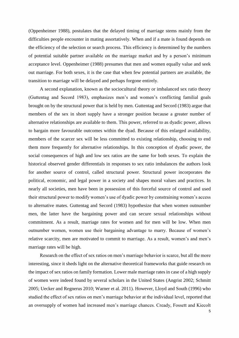
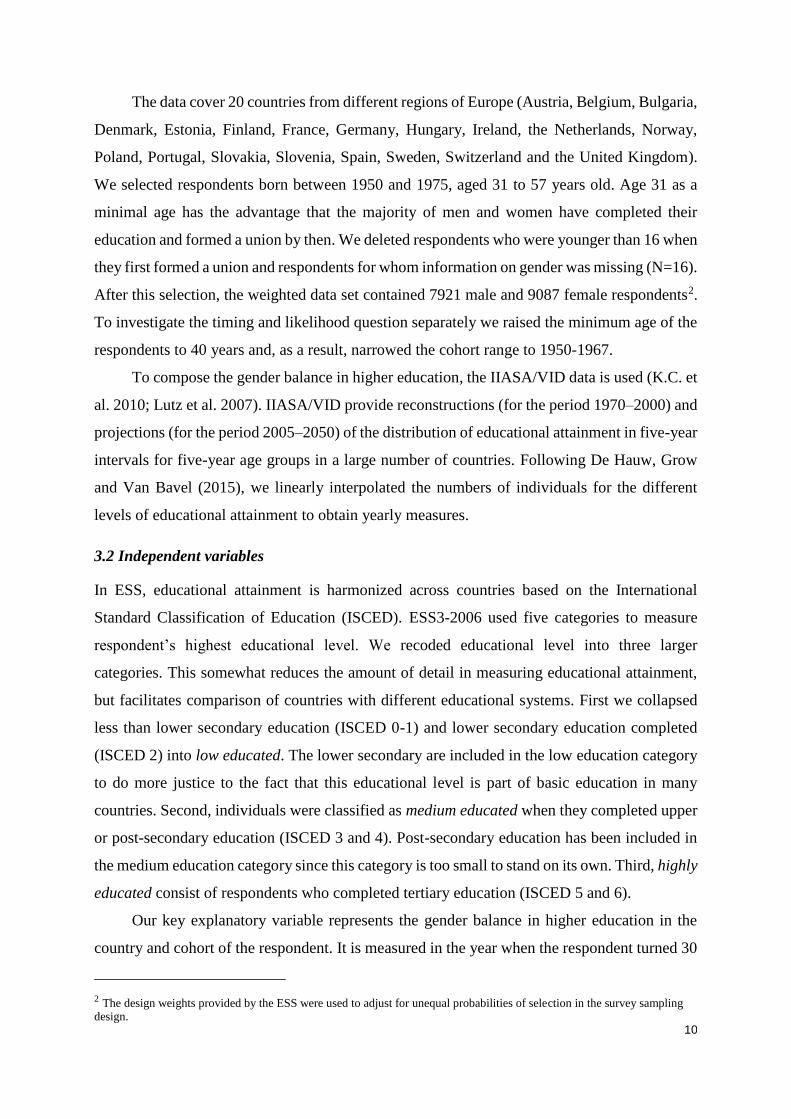
Figure 1 shows the age-cumulative proportions of first union for women by 10-year birth

cohorts. The general pattern is that there is a slight postponement of first union formation in the

later cohorts. This trend is especially noticeable in Spain, Ireland, and Portugal. As a contrast,

in Estonia, women in successive cohorts actually exhibit a decreasing age at first union

formation. The latter is in line with previous findings (Katus et al. 2007), so it does not indicate

14

a problem with the data. Also in some other Central and East European (CEE) countries, such

as Hungary, Slovenia, and Slovakia we can observe some decreases in the age at first union

formation. As of the proportions of women that have ever experienced a union by age 40, there

are no big variations across countries and across cohorts. For some countries like Great Britain

and Poland we observe a lower proportion of women ever in a union, but for most countries the

difference between cohorts is negligible.

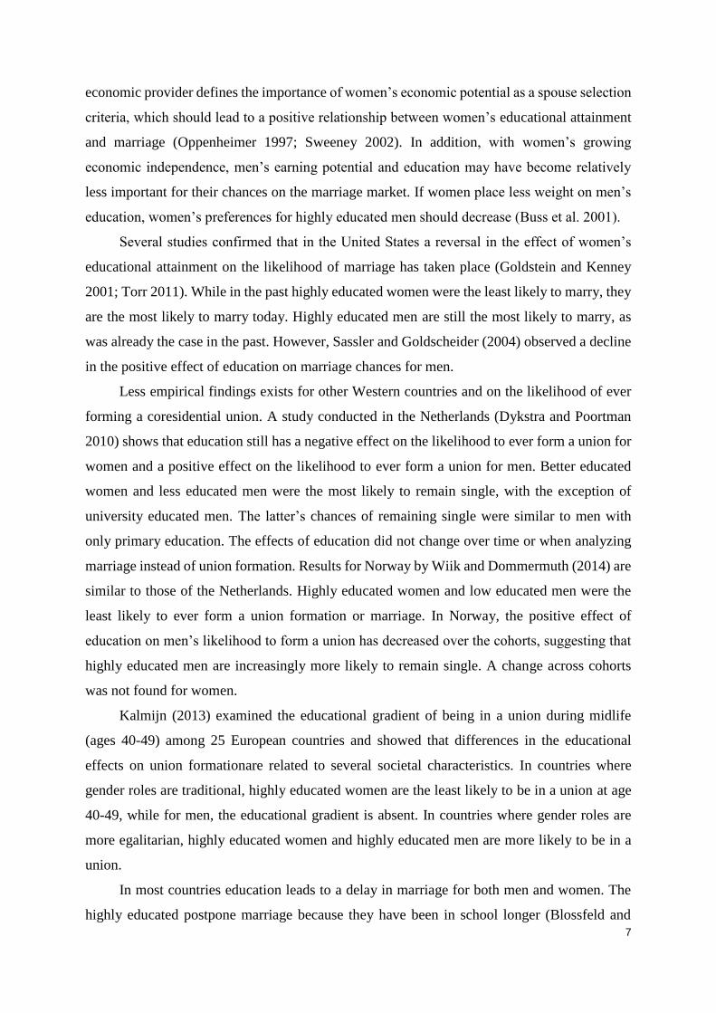
Age-cumulative proportions of men’s first union are shown in Figure 2. Postponement

of first union formation across birth cohorts is more present in Spain, Portugal, Slovenia and

Slovakia. Compared to women’s respective figures, one of the characteristics of male first union

formation is the rectangular shape of the 1950s curve, as seen for instance in Estonia, Poland,

Slovenia and Slovakia. A high proportion of first union formation occur within a narrow age

range in the first half of the twenties. Later cohorts seem to introduce more variability in the

timing of union formation and the rectangular shape is replaced with a less steep curve of

cumulative proportions.Thus, depending on the country, the timing of first union may or may

not be responsive to cohort-to-cohort changes.

15

Figure 1 Age-cumulative proportions of first union, women

Source: ESS3-2006, sampling weights, own estimation

Note: “1950” refers to the cohorts born in the 1950s, etc.

16

Figure 2 Age-cumulative proportions of first union, men

Source: ESS3-2006, sampling weights, own estimation

Note: “1950” refers to the cohorts born in the 1950s, etc.

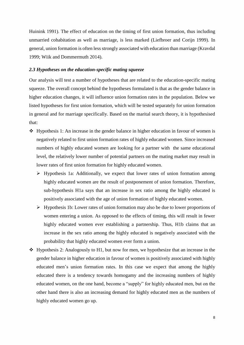
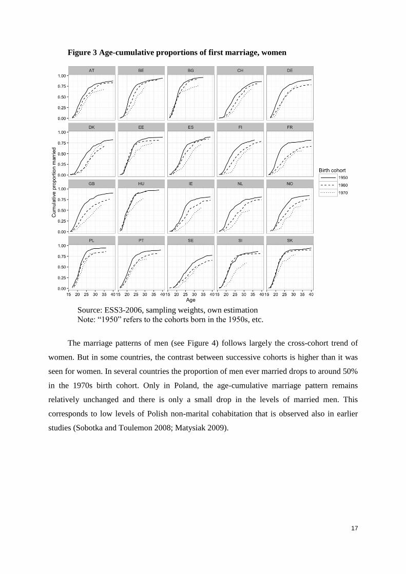
Turning now to first marriage formation, we notice more variability across countries

and across cohorts. Figure 3 depicts the age-cumulative proportions of first-married women by

10-year birth cohorts. In all countries we observe postponement of first marriage formation and

in most countries there is a decline in the proportion of ever-married women. As an example of

postponement, in Belgium the age when 50% of women have married has shifted by about five

years between the cohorts of 1950s and 1970s. The lowering proportions of ever-married,

together with increasing age at marriage, can be well seen in France, Great Britain, Norway,

and Sweden. Most Western and Northern European countries show strong postponement and

declining levels of marriage across the cohorts. Among the CEE countries, these tendencies

appear mostly in the 1970s cohort. Before 1970, marriage was widespread in these countries,

which is illustrated by an almost indistinguishable difference between the 1950s and 1960s

cohorts in some of the CEE countries.

17

Figure 3 Age-cumulative proportions of first marriage, women

Source: ESS3-2006, sampling weights, own estimation

Note: “1950” refers to the cohorts born in the 1950s, etc.

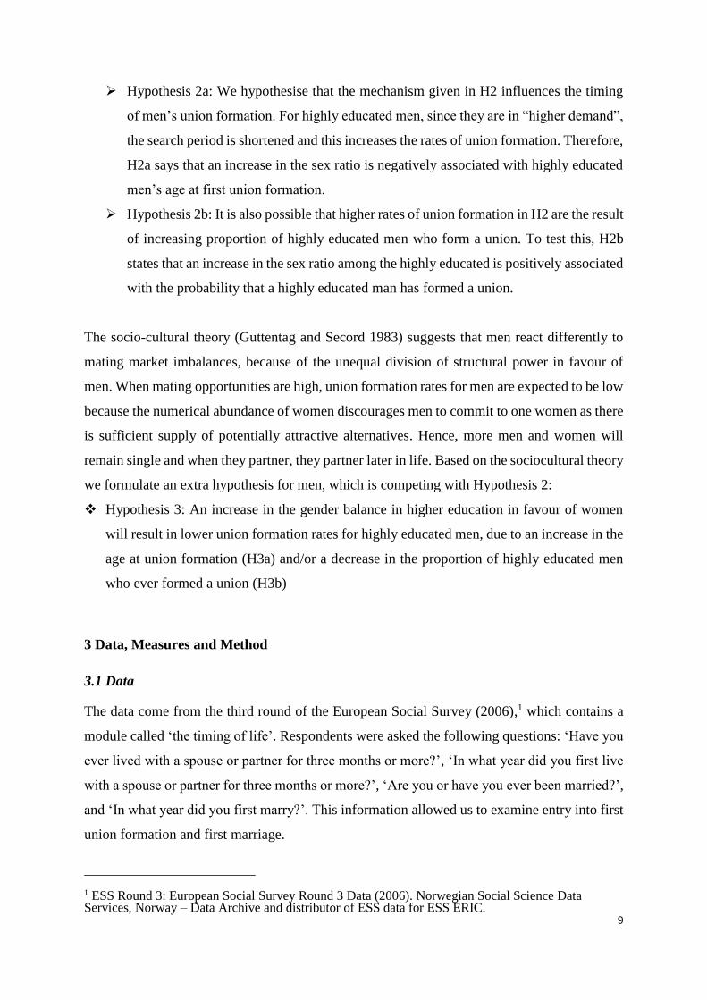
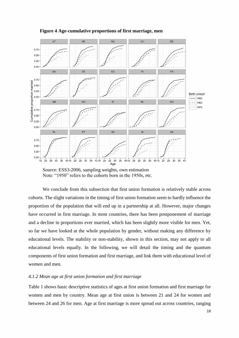
The marriage patterns of men (see Figure 4) follows largely the cross-cohort trend of

women. But in some countries, the contrast between successive cohorts is higher than it was

seen for women. In several countries the proportion of men ever married drops to around 50%

in the 1970s birth cohort. Only in Poland, the age-cumulative marriage pattern remains

relatively unchanged and there is only a small drop in the levels of married men. This

corresponds to low levels of Polish non-marital cohabitation that is observed also in earlier

studies (Sobotka and Toulemon 2008; Matysiak 2009).

18

Figure 4 Age-cumulative proportions of first marriage, men

Source: ESS3-2006, sampling weights, own estimation

Note: “1950” refers to the cohorts born in the 1950s, etc.

We conclude from this subsection that first union formation is relatively stable across

cohorts. The slight variations in the timing of first union formation seem to hardly influence the

proportion of the population that will end up in a partnership at all. However, major changes

have occurred in first marriage. In most countries, there has been postponement of marriage

and a decline in proportions ever married, which has been slightly more visible for men. Yet,

so far we have looked at the whole population by gender, without making any difference by

educational levels. The stability or non-stability, shown in this section, may not apply to all

educational levels equally. In the following, we will detail the timing and the quantum

components of first union formation and first marriage, and link them with educational level of

women and men.

4.1.2 Mean age at first union formation and first marriage

Table 1 shows basic descriptive statistics of ages at first union formation and first marriage for

women and men by country. Mean age at first union is between 21 and 24 for women and

between 24 and 26 for men. Age at first marriage is more spread out across countries, ranging

19

from 21 to 27 for women and from 24 to 29 for men. Note that in some countries, like several

CEE countries, there is very little difference between age at first union and age at first marriage.

As a contrast, the gap is much bigger in Northern European countries (for example Denmark

and Sweden). This is the result of the fact that non-marital cohabitation was more common in

North and West Europe. In CEE, where direct marriage prevailed, the difference between first

union and marriage timing is much smaller.

In addition, a relatively high mean age at first marriage is not necessarily indicative of

a relatively higher mean age at first union formation. For example Denmark shows one of the

highest mean age at first marriage, but the age at first union formation is among the lowest.

This may be due to processes such as a long premarital cohabitation period or high selectivity

into marriage (and hence a longer waiting time until marriage).

To examine the country differences in the distribution of mean age at union formation,

Figure 5 shows the respective boxplot by gender for each country. For women and men, the

countries are ordered by the mean age at first union formation, not by the median which is at

the centre of each boxplot. For women, the order of the countries indicates generally lower ages

in CEE. Also Denmark appears among countries with relatively early mean age at first union

formation. Women’s mean ages are the highest in Ireland and Spain, where the median age is

23–24. It is only in the countries of relatively high mean age at first union (Ireland, Spain,

Switzerland, and Great Britain) where the upper quartiles reach and exceed age 25. In all other

countries, three fourths of the first unions were formed before women reached age 25. Men’s

age at first union (lower part of Figure 5) are generally higher than women’s. The first quartile

for men is above age 20 in all countries except Denmark. Also, there are no countries where the

upper quartile is below age 25 and in the countries on the right side of the graph the median age

is 25 or higher. For women and men, some countries exhibit a larger range between quartiles

than others. For instance, among women in Estonia and men in Slovakia the mean age at first

union formation is distributed over a relatively narrow range, while in other countries this age

range is more spread out.

20

Table 1 Mean and standard deviation of age at first union formation and first marriage,

women and men who are at least 40 years old

Women Men

First union First marriage First union First marriage

Mean SD Mean SD Mean SD Mean SD

German

speaking

AT 22.5 4.2 24.1 4.5 24.3 4.5 26.4 4.7

CH 23.2 3.9 25.6 4.5 24.7 4.1 27.7 4.7

DE 22.3 4.0 23.8 4.8 24.9 4.8 26.8 5.1

West Europe BE 22.2 3.4 23.2 4.4 24.3 4.2 25.2 4.4

FR 22.1 3.9 23.2 4.9 24.3 4.1 26.2 4.8

NL 22.5 3.8 24.2 5.0 24.5 4.0 26.5 4.5

Nord Europe DK 21.4 3.8 26.2 5.4 23.6 4.4 29.0 4.8

FI 22.2 3.8 24.6 5.1 23.9 4.1 26.6 4.8

SE 22.0 4.6 26.6 5.1 24.1 4.4 29.0 5.4

NO 22.7 4.1 24.5 4.5 23.7 3.7 26.3 4.6

South Europe PT 22.2 4.3 22.2 4.1 23.8 3.9 23.8 3.6

ES 24.0 4.4 24.3 4.7 25.9 4.6 26.7 4.7

British Isles GB 22.4 4.4 23.2 4.8 23.7 4.2 25.5 5.0

IE 24.2 4.2 24.6 4.4 26.5 4.5 27.0 4.3

Central and

East Europe

PL 22.2 3.3 22.2 3.3 24.8 3.6 24.9 3.7

SI 22.0 3.7 22.6 4.2 24.7 4.2 25.4 4.3

SK 21.8 3.7 22.1 4.0 23.8 3.4 24.0 3.4

EE 21.9 3.3 22.4 3.6 24.0 4.1 24.1 3.6

HU 21.4 3.5 21.6 3.6 23.5 4.2 24.1 4.2

BG 21.2 3.4 21.2 3.3 23.7 4.3 23.9 4.3

Source: ESS3-2006, sampling weights.

21

Figure 5 Boxplot of age at first union formation, women and men who are at least 40 years

old

Source: ESS3-2006. Countries ordered by mean age at union formation, only unions up to age

40 considered.

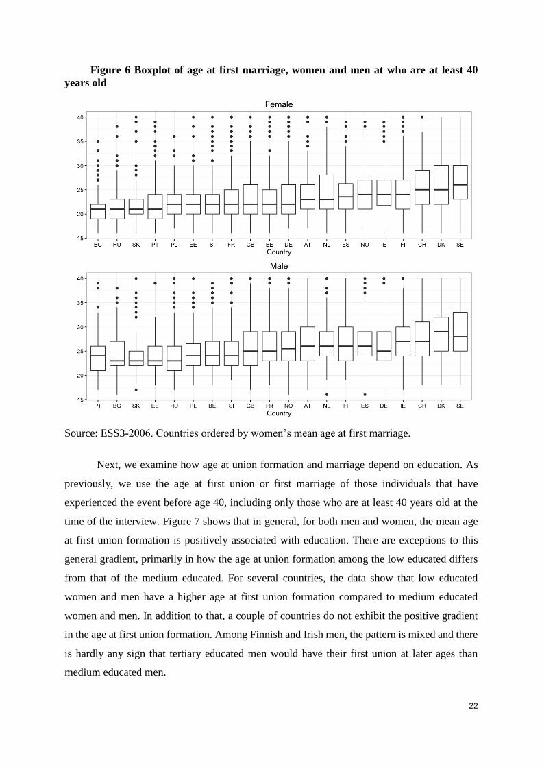
Figure 6 shows the distribution of age at first marriage for women and men in each

country. Compared to age at first union formation, age at first marriage is more heterogeneous

across countries and shows more variability within countries the age at first marriage is

relatively high. Especially among women, there is an increasing variability as the mean age at

first marriage increases. For example in Great Britain, France, the Netherlands and Sweden the

range of quartiles is around 6–7 years, whereas among countries with a low age at first marriage

the range of quartiles is much narrower. Since we are pooling cohorts over several decades, a

wide distribution of mean age at first marriage (or first union formation) may also be due to

cohort changes. The association of such change with the gender balance in higher education is

central to our research questions. A cohort view of the descriptive statistics is presented later in

this section.

22

Figure 6 Boxplot of age at first marriage, women and men at who are at least 40

years old

Source: ESS3-2006. Countries ordered by women’s mean age at first marriage.

Next, we examine how age at union formation and marriage depend on education. As

previously, we use the age at first union or first marriage of those individuals that have

experienced the event before age 40, including only those who are at least 40 years old at the

time of the interview. Figure 7 shows that in general, for both men and women, the mean age

at first union formation is positively associated with education. There are exceptions to this

general gradient, primarily in how the age at union formation among the low educated differs

from that of the medium educated. For several countries, the data show that low educated

women and men have a higher age at first union formation compared to medium educated

women and men. In addition to that, a couple of countries do not exhibit the positive gradient

in the age at first union formation. Among Finnish and Irish men, the pattern is mixed and there

is hardly any sign that tertiary educated men would have their first union at later ages than

medium educated men.

23

Figure 7 Mean age at first union formation by level of education for women and men born

in 1950s – 1975

Source: ESS3-2006. Countries ordered by mean age at first union of persons with a medium

education

In Figure 7, countries are ordered by the mean age at first union formation of persons

with a medium educated group. We notice that the difference between medium and highly

educated women tends to be larger in countries where the age at first union formation of the

medium educated is relatively low. It is possible that the age at exit from the tertiary education

causes the larger gap between the two in the countries with lower age in the medium educated

group. In countries where the medium educated have relatively high age at first union, the

additional schooling years in the tertiary education have less potential to create the gap between

the medium and highly educated.

Figure 8 shows how timing of first marriage differs by educational level. As can be seen

on the left side, there is a clear gap between medium and highly educated women’s age at first

marriage. Only in a few countries there is hardly a difference between the two categories. Age

gaps between educational levels tend to be larger for women than for men. The average age gap

between low and highly educated brides is 4 years in Bulgaria, 4.3 years in Hungary, 4.9 in

Denmark and 3.9 in Portugal. However, as with age at first union formation, there is no

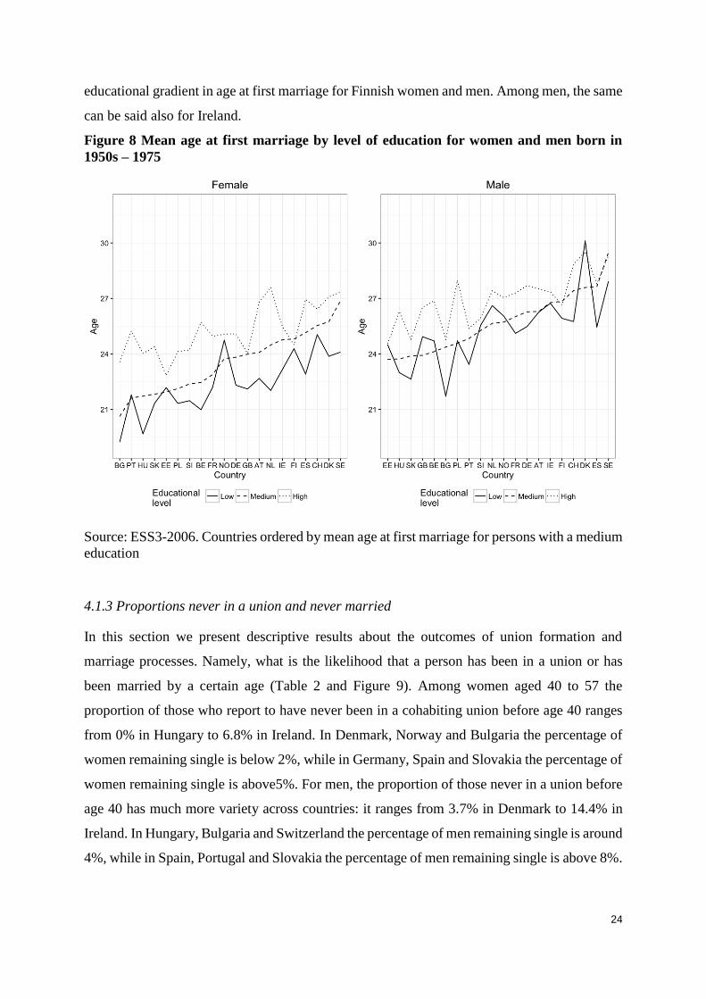
24

educational gradient in age at first marriage for Finnish women and men. Among men, the same

can be said also for Ireland.

Figure 8 Mean age at first marriage by level of education for women and men born in

1950s – 1975

Source: ESS3-2006. Countries ordered by mean age at first marriage for persons with a medium

education

4.1.3 Proportions never in a union and never married

In this section we present descriptive results about the outcomes of union formation and

marriage processes. Namely, what is the likelihood that a person has been in a union or has

been married by a certain age (Table 2 and Figure 9). Among women aged 40 to 57 the

proportion of those who report to have never been in a cohabiting union before age 40 ranges

from 0% in Hungary to 6.8% in Ireland. In Denmark, Norway and Bulgaria the percentage of

women remaining single is below 2%, while in Germany, Spain and Slovakia the percentage of

women remaining single is above5%. For men, the proportion of those never in a union before

age 40 has much more variety across countries: it ranges from 3.7% in Denmark to 14.4% in

Ireland. In Hungary, Bulgaria and Switzerland the percentage of men remaining single is around

4%, while in Spain, Portugal and Slovakia the percentage of men remaining single is above 8%.

25

Looking at the proportions of never married men and women by age 40, cross-country

patterns become more clear due to differences in the spread of unmarried cohabitation between

European countries. Among women aged 40 to 57, the proportion of never married individuals

ranges from only 2.8% in Bulgaria to 25.4% in Sweden. However, it are not only the Central

and Eastern European countries that stand out with high proportion of marriage. Also in

Belgium and Portugal the proportion of never married is relatively low with 7.3% and 8%

respectively. In Northern Europe, Germany, and France the proportion of women never married

by age 40 is at least double of these figures, being around 15%. The same applies to men. The

proportion of men never married ranges from 5% in Bulgaria to 31.5% in Sweden. In North

Europe, Germany and Ireland over one-fifth of men are not married by age 40, while in

Hungary, Slovakia and Poland this number is around 10% and lower.

Figure 9 Percentages of men and women born in 1950s – 1967 and aged 40-57 who never

cohabited nor married (never in a union) and never married before age 40

Source: ESS3-2006

26

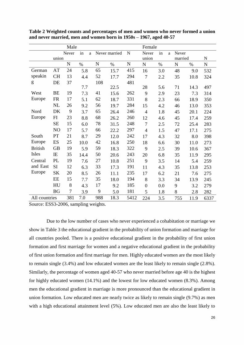
Table 2 Weighted counts and percentages of men and women who never formed a union

and never married, men and women born in 1950s – 1967, aged 40-57

Male Female

Never in a

union

Never married N Never in a

union

Never

married N

N % N % N N % N % N

German

speakin

g

AT 24 5.8 65 15.7 415 16 3.0 48 9.0 532

CH 13 4.4 52 17.7 294 7 2.2 35 10.8 324

DE 37 7.7

108 22.5

481 28 5.6 71 14.3 497

West

Europe

BE 19 7.3 41 15.6 262 9 2.9 23 7.3 314

FR 17 5.1 62 18.7 331 8 2.3 66 18.9 350

NL 26 9.2 56 19.7 284 15 4.2 46 13.0 353

Nord

Europe

DK 9 3.7 65 26.4 246 4 1.8 45 20.1 224

FI 23 8.8 68 26.2 260 12 4.6 45 17.4 259

SE 15 6.0 78 31.5 248 7 2.5 72 25.4 283

NO 17 5.7 66 22.2 297 4 1.5 47 17.1 275

South

Europe

PT 21 8.7 29 12.0 242 17 4.3 32 8.0 398

ES 25 10.0 42 16.8 250 18 6.6 30 11.0 273

British

Isles

GB 19 5.9 59 18.3 322 9 2.5 39 10.6 367

IE 35 14.4 50 20.6 243 20 6.8 35 11.9 295

Central

and East

Europe

PL 19 7.6 27 10.8 251 9 3.5 14 5.4 259

SI 12 6.3 33 17.3 191 11 4.3 35 13.8 253

SK 20 8.5 26 11.1 235 17 6.2 21 7.6 275

EE 15 7.7 35 18.0 194 8 3.3 34 13.9 245

HU 8 4.3 17 9.2 185 0 0.0 9 3.2 279

BG 7 3.9 9 5.0 181 5 1.8 8 2.8 282

All countries 381 7.0 988 18.3 5412 224 3.5 755 11.9 6337

Source: ESS3-2006, sampling weights.

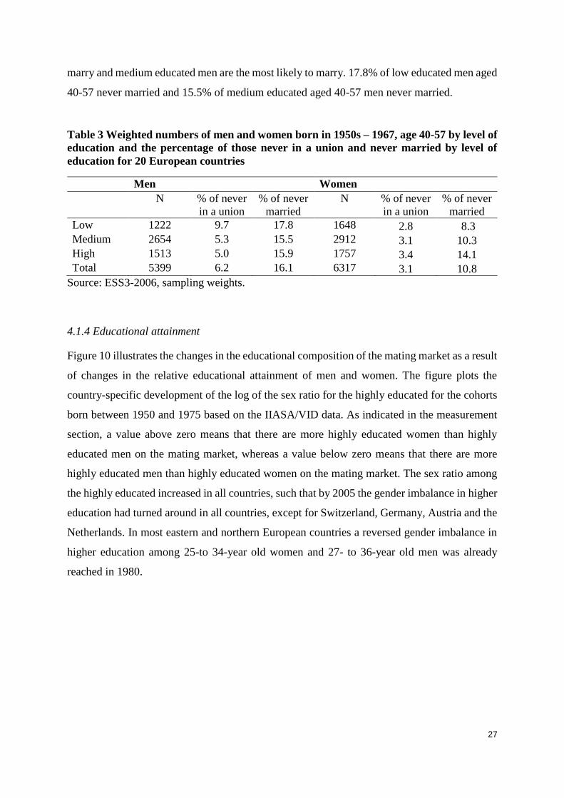
Due to the low number of cases who never experienced a cohabitation or marriage we

show in Table 3 the educational gradient in the probability of union formation and marriage for

all countries pooled. There is a positive educational gradient in the probability of first union

formation and first marriage for women and a negative educational gradient in the probability

of first union formation and first marriage for men. Highly educated women are the most likely

to remain single (3.4%) and low educated women are the least likely to remain single (2.8%).

Similarly, the percentage of women aged 40-57 who never married before age 40 is the highest

for highly educated women (14.1%) and the lowest for low educated women (8.3%). Among

men the educational gradient in marriage is more pronounced than the educational gradient in

union formation. Low educated men are nearly twice as likely to remain single (9.7%) as men

with a high educational attainment level (5%). Low educated men are also the least likely to

27

marry and medium educated men are the most likely to marry. 17.8% of low educated men aged

40-57 never married and 15.5% of medium educated aged 40-57 men never married.

Table 3 Weighted numbers of men and women born in 1950s – 1967, age 40-57 by level of

education and the percentage of those never in a union and never married by level of

education for 20 European countries

Men Women

N % of never

in a union

% of never

married

N % of never

in a union

% of never

married

Low 1222 9.7 17.8 1648 2.8 8.3

Medium 2654 5.3 15.5 2912 3.1 10.3

High 1513 5.0 15.9 1757 3.4 14.1

Total 5399 6.2 16.1 6317 3.1 10.8

Source: ESS3-2006, sampling weights.

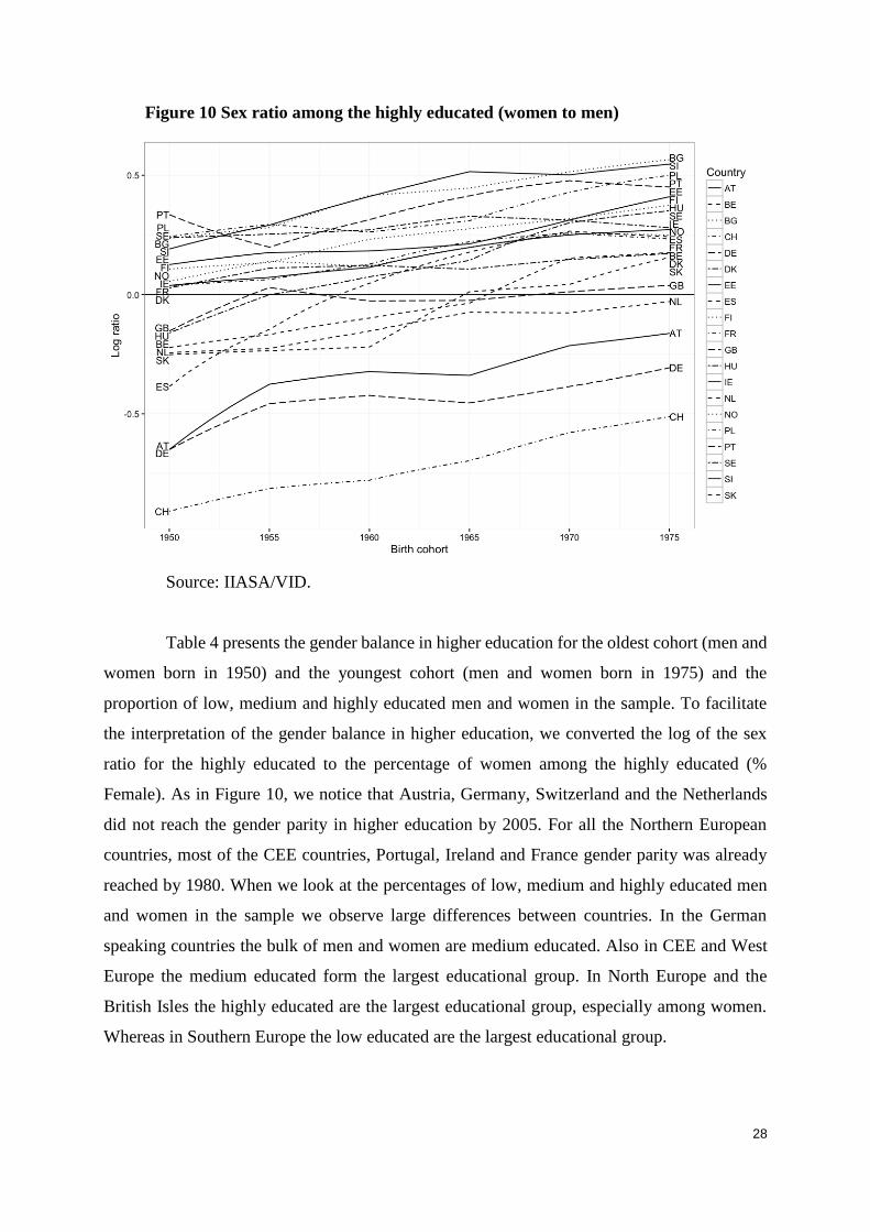
4.1.4 Educational attainment

Figure 10 illustrates the changes in the educational composition of the mating market as a result

of changes in the relative educational attainment of men and women. The figure plots the

country-specific development of the log of the sex ratio for the highly educated for the cohorts

born between 1950 and 1975 based on the IIASA/VID data. As indicated in the measurement

section, a value above zero means that there are more highly educated women than highly

educated men on the mating market, whereas a value below zero means that there are more

highly educated men than highly educated women on the mating market. The sex ratio among

the highly educated increased in all countries, such that by 2005 the gender imbalance in higher

education had turned around in all countries, except for Switzerland, Germany, Austria and the

Netherlands. In most eastern and northern European countries a reversed gender imbalance in

higher education among 25-to 34-year old women and 27- to 36-year old men was already

reached in 1980.

28

Figure 10 Sex ratio among the highly educated (women to men)

Source: IIASA/VID.

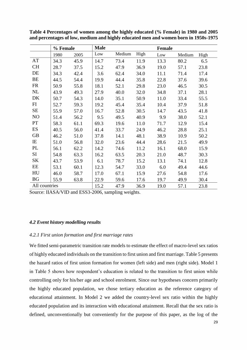
Table 4 presents the gender balance in higher education for the oldest cohort (men and

women born in 1950) and the youngest cohort (men and women born in 1975) and the

proportion of low, medium and highly educated men and women in the sample. To facilitate

the interpretation of the gender balance in higher education, we converted the log of the sex

ratio for the highly educated to the percentage of women among the highly educated (%

Female). As in Figure 10, we notice that Austria, Germany, Switzerland and the Netherlands

did not reach the gender parity in higher education by 2005. For all the Northern European

countries, most of the CEE countries, Portugal, Ireland and France gender parity was already

reached by 1980. When we look at the percentages of low, medium and highly educated men

and women in the sample we observe large differences between countries. In the German

speaking countries the bulk of men and women are medium educated. Also in CEE and West

Europe the medium educated form the largest educational group. In North Europe and the

British Isles the highly educated are the largest educational group, especially among women.

Whereas in Southern Europe the low educated are the largest educational group.

29

Table 4 Percentages of women among the highly educated (% Female) in 1980 and 2005

and percentages of low, medium and highly educated men and women born in 1950s-1975

% Female Male Female 1980 2005 Low Medium High Low Medium High

AT 34.3 45.9 14.7 73.4 11.9 13.3 80.2 6.5

CH 28.7 37.5 15.2 47.9 36.9 19.0 57.1 23.8

DE 34.3 42.4 3.6 62.4 34.0 11.1 71.4 17.4

BE 44.5 54.4 19.9 44.4 35.8 22.8 37.6 39.6

FR 50.9 55.8 18.1 52.1 29.8 23.0 46.5 30.5

NL 43.9 49.3 27.9 40.0 32.0 34.8 37.1 28.1

DK 50.7 54.3 14.0 35.1 50.9 11.0 33.4 55.5

FI 52.7 59.3 19.2 45.4 35.4 10.4 37.9 51.8

SE 55.9 57.0 16.7 52.8 30.5 14.7 43.5 41.8

NO 51.4 56.2 9.5 49.5 40.9 9.9 38.0 52.1

PT 58.3 61.1 69.3 19.6 11.0 71.7 12.9 15.4

ES 40.5 56.0 41.4 33.7 24.9 46.2 28.8 25.1

GB 46.2 51.0 37.8 14.1 48.1 38.9 10.9 50.2

IE 51.0 56.8 32.0 23.6 44.4 28.6 21.5 49.9

PL 56.1 62.2 14.2 74.6 11.2 16.1 68.0 15.9

SI 54.8 63.3 16.2 63.5 20.3 21.0 48.7 30.3

SK 43.7 53.9 6.1 78.7 15.2 13.1 74.1 12.8

EE 53.1 60.1 12.3 54.7 33.0 6.0 49.4 44.6

HU 46.0 58.7 17.0 67.1 15.9 27.6 54.8 17.6

BG 55.9 63.8 22.9 59.6 17.6 19.7 49.9 30.4

All countries 15.2 47.9 36.9 19.0 57.1 23.8

Source: IIASA/VID and ESS3-2006, sampling weights.

4.2 Event history modelling results

4.2.1 First union formation and first marriage rates

We fitted semi-parametric transition rate models to estimate the effect of macro-level sex ratios

of highly educated individuals on the transition to first union and first marriage. Table 5 presents

the hazard ratios of first union formation for women (left side) and men (right side). Model 1

in Table 5 shows how respondent’s education is related to the transition to first union while

controlling only for his/her age and school enrolment. Since our hypotheses concern primarily

the highly educated population, we chose tertiary education as the reference category of

educational attainment. In Model 2 we added the country-level sex ratio within the highly

educated population and its interaction with educational attainment. Recall that the sex ratio is

defined, unconventionally but conveniently for the purpose of this paper, as the log of the

30

number of highly educated women divided by the number of highly educated men. Also note

that including interaction effects in a regression model affects the meaning of the slope

coefficients for the interacted variables (Jaccard 2001). As a result, the significance test of the

so-called main effect of the interaction term characterizes the influence of the sex ratio when

education is set at the reference category, and conversely, the effect of education when the

logarithm of the sex ratio is zero. As the last step, in Model 3 we additionally controlled for the

birth cohort of the respondent. In all three models we included country dummies and use

country clustered robust standard errors.

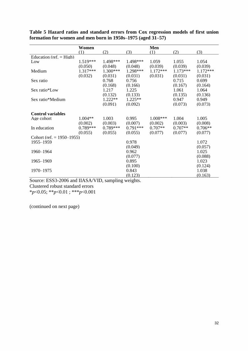
The results on the left side of Table 5 are about women. The point estimate for the sex

ratio suggests that, in line with hypothesis 1, an increase in the gender balance in higher

education to the advantage of women is associated with a lower hazard of first union formation

for highly educated women (hazard ratio values for this coefficient are below one in all models

where the sex ratio was included). However, this relationship is not statistically significant in

neither case. The only statistically significant coefficient related to the sex ratio is the

interaction with medium education (HR 1.225** in model 3). This indicates that, as the gender

balance in education turns towards an advantage for women, union formation rates of medium

educated women increase compared to union formation rates of highly educated women – and

note that rates of union formation are already higher for medium educated women in a balanced

mating market, as indicated by the hazard ratio for medium educated women compared to the

highly educated reference category (1.298 in model 3 for women). A similar pattern emerges

for low educated women, but the interaction with the sex ratio is statistically not significant.

All in all, these results contain only weak indications that the rates of union formation for highly

educated women would deteriorate with the reversal of the gender balance in education, but

they do clearly indicate that they decrease compared to the rates for women with less education.

In sum, Hypothesis 1 is hardly supported.

The results for men are on the right hand side of Table 5. The picture looks different for

men compared to women. The estimates for the sex ratio effect, not interacted so referring to

the reference category of highly educated men, are similar to the ones for women. Also here,

they are not statistically significant. A unit change in the logged sex ratio variable would lower

highly educated men’s transition rate to first union by about 25–30%. However, in contrast to

what we just observed for women, this reduction seems to apply for all three levels of education;

among men the difference in the effect of the sex ratio between the highly educated and the rest

is much smaller, if existent at all. So, all in all, the results could be seen as in line with

Hypothesis 3, implying lower union formation rates for highly educated men as the sex ratio

31

goes up. However, the evidence supporting this is very thin, as the effect is not statistically

significant and should only hold for highly educated men, according to the rationale behind

Hypothesis 3.

Furthermore, Table 5 indicates a negative educational gradient of first union formation in

a balanced market for women, but not for men. Highly educated women have the lowest hazard

of first union formation and low educated women have the highest hazard. Among men, it is

the medium educated group who have the highest rates of first union formation, producing an

inverted U-shape pattern. Low and highly educated men have statistically significant lower

rates of union formation compared to medium educated men.

Control variables in Table 5 adjust for differences due to the age cohort of the respondent

and school enrolment. Age cohort of the respondent is positively associated with the transition

rate to first union in the baseline model. That is, the model would predict a higher transition

rate for older respondents, i.e. those from earlier birth cohorts. After we add the interaction

effects between the sex ratio and education, the age coefficient loses its statistical significance,

which may be due to the fact that age and the sex ratio are correlated. The school enrolment

variable suggest a consistent difference between individuals who are out of schooling and those

who are still enrolled in education. Being “in education” has a similar influence on both women

and men; it decreases the hazard of first union formation. As of the differences between

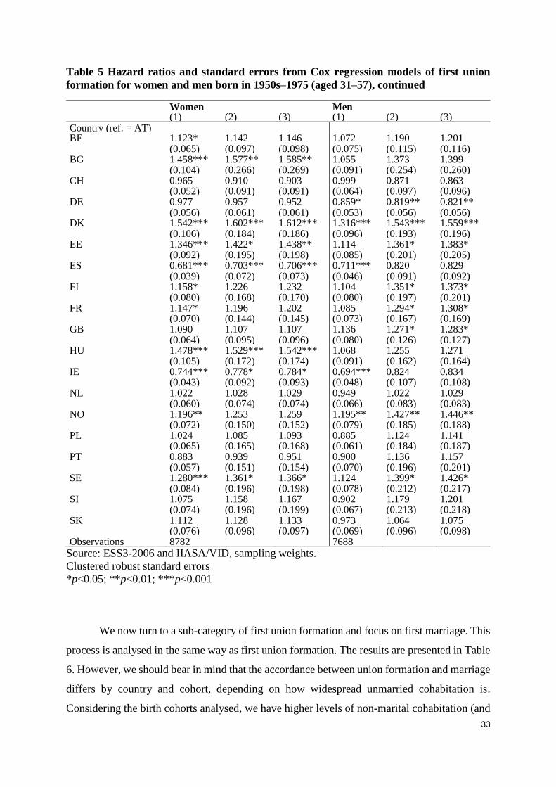
countries, these are illustrated by the respective indicator variables. For example, in the final

model we can observe relatively higher transition rates for both sexes for Denmark, Estonia,

and Sweden (compared to the baseline which is Austria). On the other hand, when only women

are considered, Spain and Ireland show relatively lower hazard of first union compared to the

reference country.

32

Table 5 Hazard ratios and standard errors from Cox regression models of first union

formation for women and men born in 1950s–1975 (aged 31–57)

Women Men (1) (2) (3) (1) (2) (3) Education (ref. = High) Low 1.519*** 1.498*** 1.498*** 1.059 1.055 1.054 (0.050) (0.048) (0.048) (0.039) (0.039) (0.039) Medium 1.317*** 1.300*** 1.298*** 1.172*** 1.173*** 1.172*** (0.032) (0.031) (0.031) (0.031) (0.031) (0.031) Sex ratio 0.768 0.756 0.715 0.699 (0.168) (0.166) (0.167) (0.164) Sex ratio*Low 1.217 1.225 1.061 1.064 (0.132) (0.133) (0.135) (0.136) Sex ratio*Medium 1.222** 1.225** 0.947 0.949 (0.091) (0.092) (0.073) (0.073) Control variables Age cohort 1.004** 1.003 0.995 1.008*** 1.004 1.005 (0.002) (0.003) (0.007) (0.002) (0.003) (0.008) In education 0.789*** 0.789*** 0.791*** 0.707** 0.707** 0.706** (0.055) (0.055) (0.055) (0.077) (0.077) (0.077) Cohort (ref. = 1950–1955) 1955–1959 0.978 1.072 (0.049) (0.057) 1960–1964 0.962 1.025 (0.077) (0.088) 1965–1969 0.895 1.023 (0.100) (0.124) 1970–1975 0.843 1.038 (0.123) (0.163)

Source: ESS3-2006 and IIASA/VID, sampling weights.

Clustered robust standard errors

*p<0.05; **p<0.01 ; ***p<0.001

(continued on next page)

33

Table 5 Hazard ratios and standard errors from Cox regression models of first union

formation for women and men born in 1950s–1975 (aged 31–57), continued

Women Men (1) (2) (3) (1) (2) (3) Country (ref. = AT) BE 1.123* 1.142 1.146 1.072 1.190 1.201 (0.065) (0.097) (0.098) (0.075) (0.115) (0.116) BG 1.458*** 1.577** 1.585** 1.055 1.373 1.399 (0.104) (0.266) (0.269) (0.091) (0.254) (0.260) CH 0.965 0.910 0.903 0.999 0.871 0.863 (0.052) (0.091) (0.091) (0.064) (0.097) (0.096) DE 0.977 0.957 0.952 0.859* 0.819** 0.821** (0.056) (0.061) (0.061) (0.053) (0.056) (0.056) DK 1.542*** 1.602*** 1.612*** 1.316*** 1.543*** 1.559*** (0.106) (0.184) (0.186) (0.096) (0.193) (0.196) EE 1.346*** 1.422* 1.438** 1.114 1.361* 1.383* (0.092) (0.195) (0.198) (0.085) (0.201) (0.205) ES 0.681*** 0.703*** 0.706*** 0.711*** 0.820 0.829 (0.039) (0.072) (0.073) (0.046) (0.091) (0.092) FI 1.158* 1.226 1.232 1.104 1.351* 1.373* (0.080) (0.168) (0.170) (0.080) (0.197) (0.201) FR 1.147* 1.196 1.202 1.085 1.294* 1.308* (0.070) (0.144) (0.145) (0.073) (0.167) (0.169) GB 1.090 1.107 1.107 1.136 1.271* 1.283* (0.064) (0.095) (0.096) (0.080) (0.126) (0.127) HU 1.478*** 1.529*** 1.542*** 1.068 1.255 1.271 (0.105) (0.172) (0.174) (0.091) (0.162) (0.164) IE 0.744*** 0.778* 0.784* 0.694*** 0.824 0.834 (0.043) (0.092) (0.093) (0.048) (0.107) (0.108) NL 1.022 1.028 1.029 0.949 1.022 1.029 (0.060) (0.074) (0.074) (0.066) (0.083) (0.083) NO 1.196** 1.253 1.259 1.195** 1.427** 1.446** (0.072) (0.150) (0.152) (0.079) (0.185) (0.188) PL 1.024 1.085 1.093 0.885 1.124 1.141 (0.065) (0.165) (0.168) (0.061) (0.184) (0.187) PT 0.883 0.939 0.951 0.900 1.136 1.157 (0.057) (0.151) (0.154) (0.070) (0.196) (0.201) SE 1.280*** 1.361* 1.366* 1.124 1.399* 1.426* (0.084) (0.196) (0.198) (0.078) (0.212) (0.217) SI 1.075 1.158 1.167 0.902 1.179 1.201 (0.074) (0.196) (0.199) (0.067) (0.213) (0.218) SK 1.112 1.128 1.133 0.973 1.064 1.075 (0.076) (0.096) (0.097) (0.069) (0.096) (0.098) Observations 8782 7688

Source: ESS3-2006 and IIASA/VID, sampling weights.

Clustered robust standard errors

*p<0.05; **p<0.01; ***p<0.001

We now turn to a sub-category of first union formation and focus on first marriage. This

process is analysed in the same way as first union formation. The results are presented in Table

6. However, we should bear in mind that the accordance between union formation and marriage

differs by country and cohort, depending on how widespread unmarried cohabitation is.

Considering the birth cohorts analysed, we have higher levels of non-marital cohabitation (and

34

lower rates of marriage, respectively) in Nord and West European countries and high rates of

marriages in East European countries, as shown in the descriptive part. This must be kept in

mind, as high rates and early age of marriage coincided with a gender balance in higher

education that was already in favour of women in the 1950s birth cohorts. In Table 6, models

for women show a higher relative risk of marriage associated with an increase in the logged sex

ratio of the highly educated. For highly educated women the transition rate to marriage goes up

very strongly as the sex ratio increases (the hazard ratio is 1.995** in model 2 and 1.939** in

model 3). This finding is strongly at odds with Hypothesis 1, according to which women’s

union formation rates, including marriage, should go down as women become a larger majority

among the highly educated.

Although not shown in the table, the statistical significance of these ratios disappears

when we do not control for the age of the respondent, which again highlights the fact that the

age cohort and the sex ratio variables are strongly correlated. Apart from that, we also note that

there seems to be a positive correlation between our sex ratio variable and marriage rates across

countries. This suggests that, in countries where marriage rates are relatively high, they are

particularly high among the highly educated (compared to highly educated in other countries),

and that such is particularly the case in countries where women have a high advantage in

education. Again, this is clearly at odds with the marriage variant of Hypothesis 1.

The models for men, on the right hand side of Table 6, indicate that an increase in the

logged sex ratio of the highly educated population reduces the rate of transition to marriage for

the low educated compared to the highly educated (hazard ratio figures 0.737* and 0.736*). For

the highly educated, if anything, there is an increase in the marriage rate as the sex ratio

increases (which would be in line with Hypothesis 2), but the coefficients do not reach the level

of statistical significance. All in all, we find hardly support for Hypothesis 2 and no support for

Hypothesis 3. The most important finding here is that marriages rates of low educated men

decrease as women gain an advantage in higher education.

Regarding the other variables in the models in Table 6, level of education yields

relatively similar results to first marriage as to first union formation. For women there is a clear

and consistent negative gradient. The low educated show hazard rates that are increased by

about half compared to highly educated women. The difference in rates between highly

educated and medium educated women is about a third of the level of the former. On the right

side of the table, for men, only a medium level of education shows a statistically significant

difference from the tertiary educational level, producing a similar pattern that was observed for

first union formation.

35

Among the control variables, age remains a significant predictor of marriage even after

including country-level sex ratio of the highly educated and 5-year birth cohort. This may be

an indication that in our data, marriage rates are more sensitive to the birth cohort of the

respondent, as marriage was more common in older cohorts.

Table 6 Hazard ratios and standard errors from Cox regression models of first marriage

for women and men born in 1950s–1975 (aged 31–57)

Women Men (1) (2) (3) (1) (2) (3) Education (ref. = Highly educated) Low educated 1.515*** 1.523*** 1.525*** 1.012 1.023 1.019 (0.055) (0.055) (0.055) (0.041) (0.041) (0.041) Medium educated 1.316*** 1.323*** 1.319*** 1.103** 1.101** 1.099** (0.037) (0.037) (0.037) (0.034) (0.034) (0.034) Sex ratio*Education Sex ratio 1.995** 1.939** 1.178 1.122 (0.492) (0.484) (0.314) (0.303) Sex ratio*Low 0.840 0.847 0.737* 0.736* (0.103) (0.103) (0.105) (0.105) Sex ratio*Medium 0.986 0.989 0.919 0.919 (0.084) (0.085) (0.078) (0.079) Control variables Age cohort 1.030*** 1.038*** 1.034*** 1.038*** 1.039*** 1.036*** (0.002) (0.003) (0.008) (0.002) (0.003) (0.010) In education 0.894 0.892 0.892 0.718** 0.710** 0.714** (0.065) (0.065) (0.064) (0.091) (0.090) (0.092) Cohort (ref. = 1950-1954) 1955-1959 1.081 1.092 (0.061) (0.066) 1960-1964 1.082 1.070 (0.097) (0.105) 1965-1969 0.989 1.033 (0.125) (0.144) 1970-1975 0.922 0.913 (0.153) (0.165)

Source: ESS3-2006 and IIASA/VID, sampling weights.

Clustered robust standard errors.

*p<0.05; **p<0.01

(continued on next page)

36

Table 6 Hazard ratios and standard errors from Cox regression models of first marriage

for women and men born in 1950s–1975 (aged 31–57), continued

Women Men (1) (2) (3) (1) (2) (3)

Country (ref. = AT) BE 1.243*** 1.034 1.051 1.121 2.289*** 1.338** (0.081) (0.098) (0.100) (0.089) (0.207) (0.141) BG 1.972*** 1.229 1.266 1.684*** 9.093*** 2.197*** (0.157) (0.232) (0.242) (0.163) (1.294) (0.452) CH 0.862** 1.115 1.110 0.945 0.393*** 0.849 (0.048) (0.124) (0.124) (0.063) (0.033) (0.101) DE 0.918 0.999 0.998 0.833** 0.662*** 0.837* (0.055) (0.068) (0.068) (0.057) (0.046) (0.062) DK 0.735*** 0.551*** 0.562*** 0.721*** 2.088*** 0.874 (0.050) (0.069) (0.071) (0.052) (0.203) (0.117) EE 1.192* 0.825 0.850 1.191 4.521*** 1.546** (0.096) (0.129) (0.135) (0.111) (0.560) (0.257) ES 0.887 0.691** 0.703** 0.896 2.290*** 1.140 (0.056) (0.078) (0.081) (0.065) (0.218) (0.136) FI 0.806** 0.560*** 0.574*** 0.793** 3.016*** 1.007 (0.056) (0.084) (0.087) (0.060) (0.339) (0.161) FR 0.802** 0.587*** 0.599*** 0.890 2.874*** 1.127 (0.056) (0.079) (0.082) (0.066) (0.301) (0.160) GB 1.059 0.874 0.883 1.017 2.222*** 1.240* (0.068) (0.083) (0.085) (0.079) (0.203) (0.134) HU 1.807*** 1.376* 1.414** 1.360** 3.960*** 1.719*** (0.147) (0.174) (0.181) (0.129) (0.453) (0.245) IE 0.873* 0.640*** 0.654** 0.831* 2.687*** 1.062 (0.059) (0.085) (0.088) (0.065) (0.287) (0.153) NL 0.826** 0.730*** 0.739*** 0.858* 1.423*** 0.988 (0.052) (0.056) (0.057) (0.066) (0.121) (0.091) NO 0.822** 0.597*** 0.608*** 0.825** 2.742*** 1.054 (0.055) (0.080) (0.083) (0.061) (0.286) (0.151) PL 1.438*** 0.937 0.967 1.441*** 6.814*** 1.877*** (0.104) (0.162) (0.169) (0.113) (0.833) (0.341) PT 1.129 0.740 0.766 1.263** 6.916*** 1.910*** (0.081) (0.134) (0.140) (0.114) (0.930) (0.362) SE 0.567*** 0.380*** 0.388*** 0.556*** 2.358*** 0.727 (0.038) (0.061) (0.064) (0.042) (0.272) (0.124) SI 1.009 0.631* 0.650* 0.919 5.349*** 1.277 (0.081) (0.120) (0.125) (0.083) (0.722) (0.257) SK 1.476*** 1.270** 1.298** 1.504*** 2.774*** 1.786*** (0.108) (0.116) (0.120) (0.122) (0.254) (0.184) Observations 8756 7664

Source: ESS3-2006 and IIASA/VID, sampling weights.

Clustered robust standard errors.

*p<0.05; **p<0.01

4.2.2 Probability of first union formation and first marriage

Rates of union formation and entry into marriage consist of two components: the probability of

ever making the transition and the timing of the event. In this section we focus on the probability

that the first union or marriage takes place at all before age 40. The results of binary logistic

regressions of union formation are shown in Table 7.

37

Both for women and men, the estimates for the effect of the sex ratio as well as for the

interaction with educational level remain below the level of statistical significance. The results

do suggest that an increase in the sex ratio may lower the probability of union formation for

highly educated women and men, thus supporting the sociocultural theory (Guttentag and

Secord 1983) or H1b and H3b, but the standard errors are too large compared to the point

estimates to make any reliable claims about this.

If there is a negative educational gradient in the likelihood of union formation for

women, is does not appear as statistically significant in our data. Among men, however, it is

the low educated group who clearly exhibit the lowest likelihood of union formation, and this

differences appears statistically significant.

The control variables age and 5-year birth cohort (the last birth cohort has been dropped

due to age limitations of the subsample) produce no statistically significant results. When

individuals are still enrolled in education at the time of interview, their likelihood to have

experienced a co-residential union is lower, especially for men. Country coefficients for

Hungarian women are missing due to lack of observations for those never been in a union.

38

Table 7 Logistic regression of first union formation, women and men born in 1950s–1967

(age 40-57), odds ratios and standard errors

Women Men (1) (2) (1) (2) Education (ref. High)

Low 1.319 1.291 0.502*** 0.507***

(0.287) (0.281) (0.092) (0.092)

Medium 1.267 1.250 0.920 0.945

(0.193) (0.177) (0.174) (0.186) Sex ratio 0.180 0.573 (0.186) (1.080) Sex ratio*Low 2.793 1.820 (2.102) (1.102) Sex ratio*Medium 2.200 1.903 (0.989) (1.092) Age cohort 0.975 0.961 1.078 1.077 (0.044) (0.047) (0.046) (0.053) In education 0.441** 0.450** 0.184*** 0.185*** (0.110) (0.113) (0.060) (0.060) Cohort (ref. 1950-1954) 1955-1959 0.974 0.982 1.383 1.385 (0.284) (0.284) (0.358) (0.359) 1960-1964 0.611 0.613 1.662 1.664 (0.364) (0.369) (0.679) (0.685) 1965-1969 0.654 0.652 2.144 2.152 (0.499) (0.506) (1.189) (1.201) Observations 5772 5193 5193

Source: ESS3-2006 and IIASA/VID, sampling weights.

Clustered robust standard errors.

*p<0.05; **p<0.01; ***p<0.001

(continued on next page)

39

Table 7 Logistic regression of first union formation, women and men born in 1950s–1967

(age 40-57), odds ratios and standard errors, continued

Women Men (1) (2) (1) (2) Country (ref. = AT) BE 1.088 1.357 0.763*** 0.754 (0.101) (0.394) (0.045) (0.367) BG 1.794*** 3.893 1.446*** 1.454 (0.186) (2.775) (0.085) (1.978) CH 1.316*** 0.830 1.246*** 1.148 (0.0942) (0.299) (0.071) (0.877) DE 0.513*** 0.444*** 0.629*** 0.592* (0.031) (0.052) (0.039) (0.125) DK 2.441*** 3.966** 1.762*** 1.810 (0.261) (1.900) (0.150) (1.600) EE 0.992 1.808 0.685*** 0.696 (0.090) (0.991) (0.029) (0.714) ES 0.435*** 0.617 0.633*** 0.633 (0.046) (0.249) (0.048) (0.431) FI 0.679*** 1.246 0.635*** 0.650 (0.076) (0.700) (0.041) (0.689) FR 1.412*** 2.332 1.037 1.049 (0.107) (1.154) (0.051) (0.975) GB 1.288* 1.741 1.142 1.142 (0.166) (0.663) (0.111) (0.744) HU 1.314*** 1.304 (0.048) (0.987) IE 0.489*** 0.810 0.385*** 0.392 (0.050) (0.403) (0.027) (0.369) NL 0.756** 0.900 0.640*** 0.628 (0.066) (0.228) (0.040) (0.246) NO 2.275*** 3.850** 1.053 1.079 (0.231) (1.930) (0.071) (1.018) PL 0.836* 1.590 0.714*** 0.707 (0.065) (1.021) (0.029) (0.850) PT 0.647** 1.240 0.871 0.872 (0.098) (0.886) (0.082) (1.165) SE 1.323** 2.659 0.943 0.962 (0.121) (1.681) (0.055) (1.165) SI 0.733** 1.628 1.019 1.027 (0.071) (1.182) (0.044) (1.432) SK 0.436*** 0.533** 0.589*** 0.585 (0.022) (0.121) (0.023) (0.226) Observations 5772 5193

Source: ESS3-2006 and IIASA/VID, sampling weights.

Clustered robust standard errors.

*p<0.05; **p<0.01; ***p<0.001

The results for the likelihood of ever been married before age 40 are shown in Table 8.

A major difference compared to union formation is found in the effect of the logged sex ratio

for the reference category of highly educated. An increase in the sex ratio among the highly

educated results in much higher odds of ever been married before age 40 for highly educated

women. This goes against our hypothesis about the levels of ever married and sex ratio (H1b).

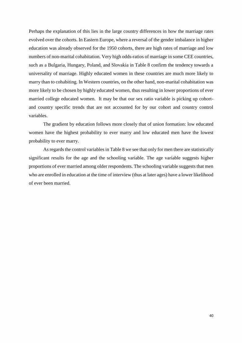
40

Perhaps the explanation of this lies in the large country differences in how the marriage rates

evolved over the cohorts. In Eastern Europe, where a reversal of the gender imbalance in higher

education was already observed for the 1950 cohorts, there are high rates of marriage and low

numbers of non-marital cohabitation. Very high odds-ratios of marriage in some CEE countries,

such as a Bulgaria, Hungary, Poland, and Slovakia in Table 8 confirm the tendency towards a

universality of marriage. Highly educated women in these countries are much more likely to

marry than to cohabiting. In Western countries, on the other hand, non-marital cohabitation was

more likely to be chosen by highly educated women, thus resulting in lower proportions of ever

married college educated women. It may be that our sex ratio variable is picking up cohort-

and country specific trends that are not accounted for by our cohort and country control

variables.

The gradient by education follows more closely that of union formation: low educated

women have the highest probability to ever marry and low educated men have the lowest

probability to ever marry.

As regards the control variables in Table 8 we see that only for men there are statistically

significant results for the age and the schooling variable. The age variable suggests higher

proportions of ever married among older respondents. The schooling variable suggests that men

who are enrolled in education at the time of interview (thus at later ages) have a lower likelihood

of ever been married.

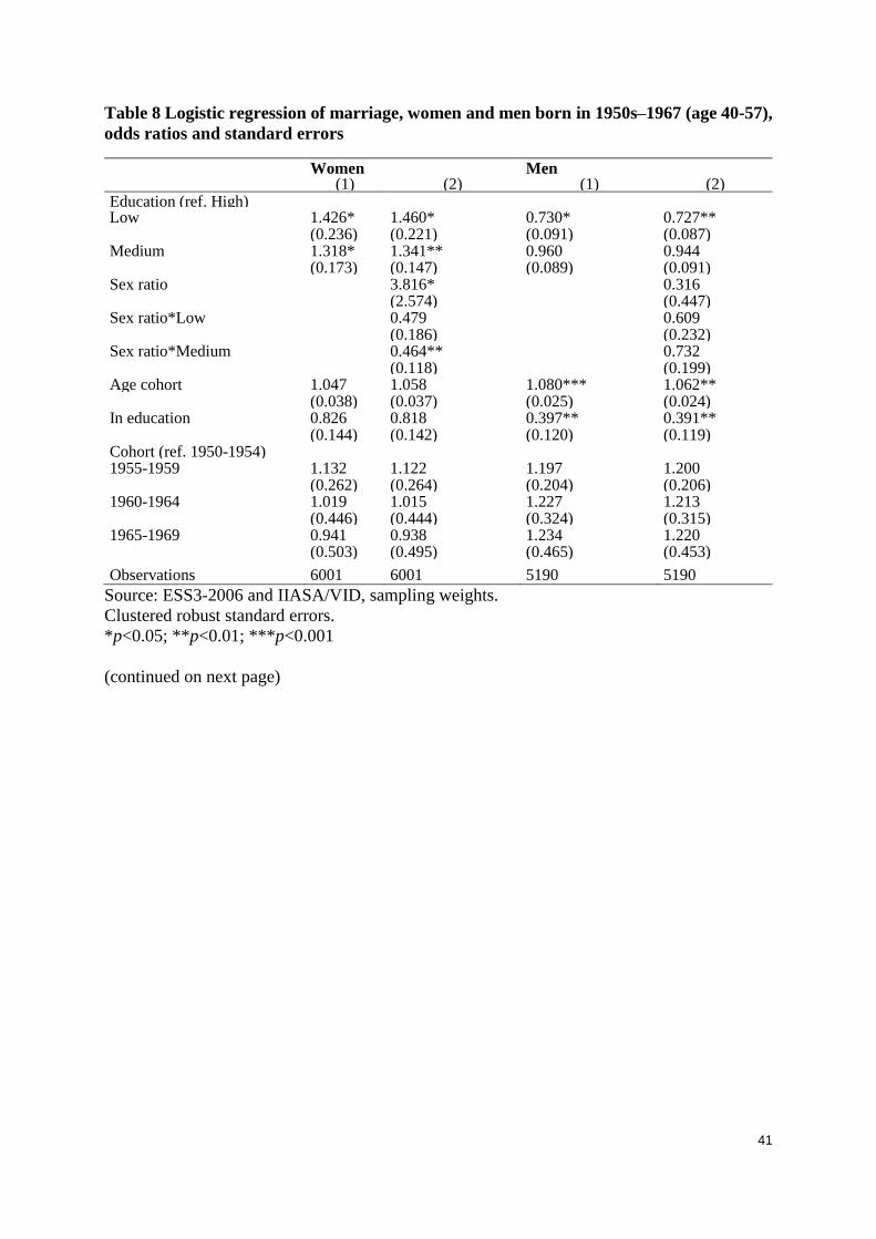
41

Table 8 Logistic regression of marriage, women and men born in 1950s–1967 (age 40-57),

odds ratios and standard errors

Women Men (1) (2) (1) (2)

Education (ref. High) Low 1.426* 1.460* 0.730* 0.727** (0.236) (0.221) (0.091) (0.087) Medium 1.318* 1.341** 0.960 0.944 (0.173) (0.147) (0.089) (0.091) Sex ratio 3.816* 0.316 (2.574) (0.447) Sex ratio*Low 0.479 0.609 (0.186) (0.232) Sex ratio*Medium 0.464** 0.732 (0.118) (0.199) Age cohort 1.047 1.058 1.080*** 1.062** (0.038) (0.037) (0.025) (0.024) In education 0.826 0.818 0.397** 0.391** (0.144) (0.142) (0.120) (0.119) Cohort (ref. 1950-1954) 1955-1959 1.132 1.122 1.197 1.200 (0.262) (0.264) (0.204) (0.206) 1960-1964 1.019 1.015 1.227 1.213 (0.446) (0.444) (0.324) (0.315) 1965-1969 0.941 0.938 1.234 1.220 (0.503) (0.495) (0.465) (0.453)

Observations 6001 6001 5190 5190

Source: ESS3-2006 and IIASA/VID, sampling weights.

Clustered robust standard errors.

*p<0.05; **p<0.01; ***p<0.001

(continued on next page)

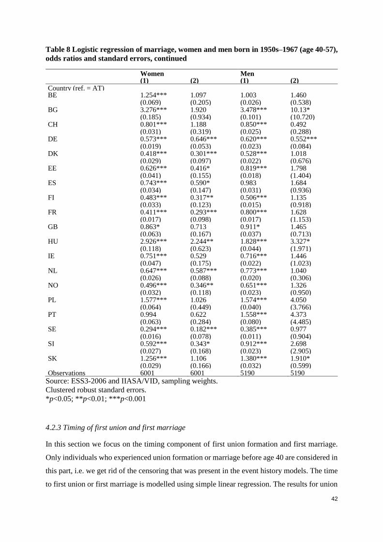
42

Table 8 Logistic regression of marriage, women and men born in 1950s–1967 (age 40-57),

odds ratios and standard errors, continued

Women Men (1) (2) (1) (2) Country (ref. = AT) BE 1.254*** 1.097 1.003 1.460 (0.069) (0.205) (0.026) (0.538) BG 3.276*** 1.920 3.478*** 10.13* (0.185) (0.934) (0.101) (10.720) CH 0.801*** 1.188 0.850*** 0.492 (0.031) (0.319) (0.025) (0.288) DE 0.573*** 0.646*** 0.620*** 0.552*** (0.019) (0.053) (0.023) (0.084) DK 0.418*** 0.301*** 0.528*** 1.018 (0.029) (0.097) (0.022) (0.676) EE 0.626*** 0.416* 0.819*** 1.798 (0.041) (0.155) (0.018) (1.404) ES 0.743*** 0.590* 0.983 1.684 (0.034) (0.147) (0.031) (0.936) FI 0.483*** 0.317** 0.506*** 1.135 (0.033) (0.123) (0.015) (0.918) FR 0.411*** 0.293*** 0.800*** 1.628 (0.017) (0.098) (0.017) (1.153) GB 0.863* 0.713 0.911* 1.465 (0.063) (0.167) (0.037) (0.713) HU 2.926*** 2.244** 1.828*** 3.327* (0.118) (0.623) (0.044) (1.971) IE 0.751*** 0.529 0.716*** 1.446 (0.047) (0.175) (0.022) (1.023) NL 0.647*** 0.587*** 0.773*** 1.040 (0.026) (0.088) (0.020) (0.306) NO 0.496*** 0.346** 0.651*** 1.326 (0.032) (0.118) (0.023) (0.950) PL 1.577*** 1.026 1.574*** 4.050 (0.064) (0.449) (0.040) (3.766) PT 0.994 0.622 1.558*** 4.373 (0.063) (0.284) (0.080) (4.485) SE 0.294*** 0.182*** 0.385*** 0.977 (0.016) (0.078) (0.011) (0.904) SI 0.592*** 0.343* 0.912*** 2.698 (0.027) (0.168) (0.023) (2.905) SK 1.256*** 1.106 1.380*** 1.910* (0.029) (0.166) (0.032) (0.599) Observations 6001 6001 5190 5190

Source: ESS3-2006 and IIASA/VID, sampling weights.

Clustered robust standard errors.

*p<0.05; **p<0.01; ***p<0.001

4.2.3 Timing of first union and first marriage

In this section we focus on the timing component of first union formation and first marriage.

Only individuals who experienced union formation or marriage before age 40 are considered in

this part, i.e. we get rid of the censoring that was present in the event history models. The time

to first union or first marriage is modelled using simple linear regression. The results for union

43

formation are shown in Table 9 and the coefficients in the table can be interpreted as change in

years in the age at first union formation.

Both for women and men, none of the coefficients of the terms related to the sex ratio

are statistically significant because the standard errors are very large. Nonetheless, the direction

of the coefficients suggests that a unit increase in the logged sex ratio would be associated with

about half a year postponement of first union formation for highly educated women, while the

medium and low educated would not be similarly affected. As opposed to that, for highly

educated men a unit increase in the logged sex ratio would mean a slight decrease in the age of

first union formation. While the interaction results for women and men may indicate some

support for the proposed association between the sex ratio and the timing of unions (H1a and

H2a), the great uncertainty of the estimated coefficients implies that we do not find support in

our data for any of these hypotheses.

Education shows a consistent positive gradient both for women and men. Low educated

women form their first union more than two years earlier than highly educated women. The gap

between medium educated women and highly educated women is over one year. Similar

association holds for men, although the timing gap between low and highly educated men and

low and medium educated men is much smaller. Except the country indicators, none of the

control variables in Table 9 show statistically significant differences.

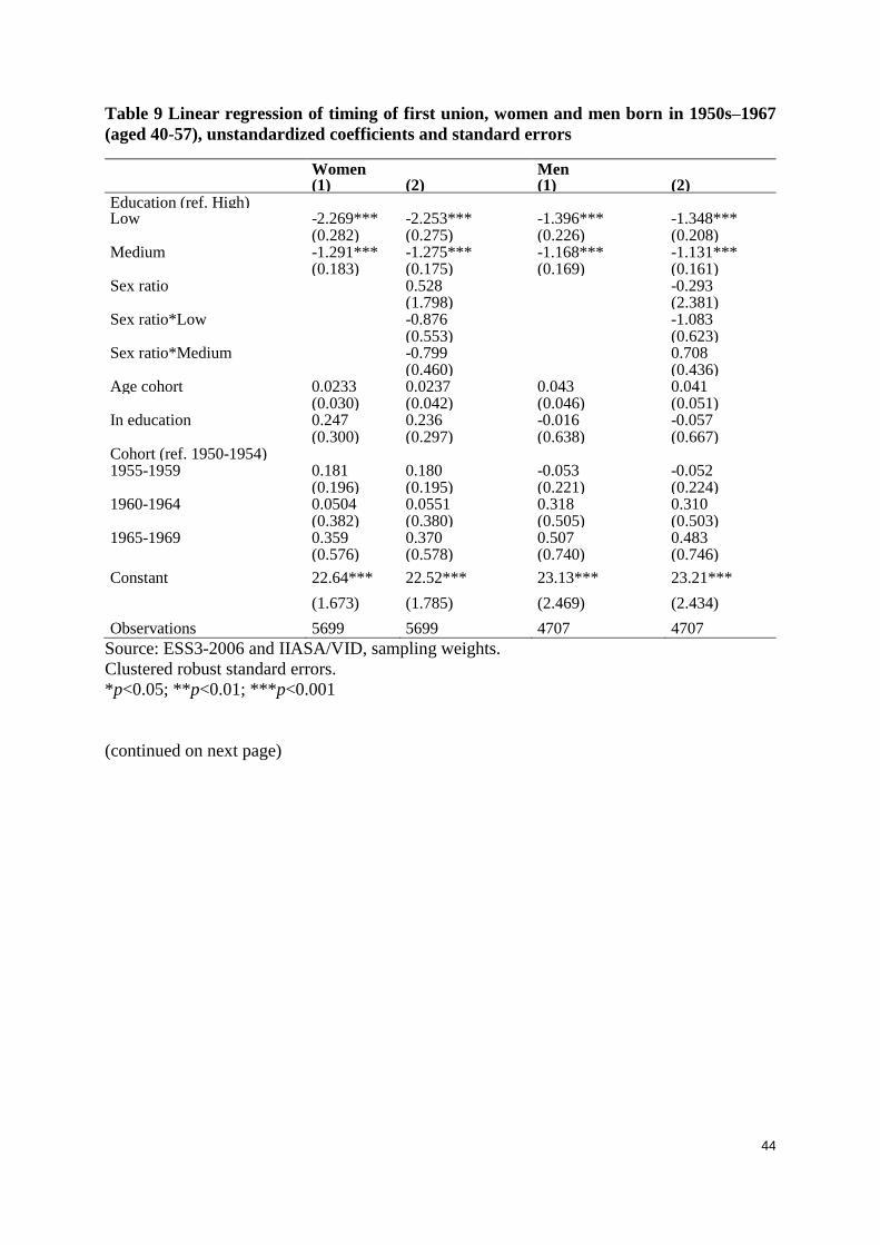
44

Table 9 Linear regression of timing of first union, women and men born in 1950s–1967

(aged 40-57), unstandardized coefficients and standard errors

Women Men (1) (2) (1) (2) Education (ref. High) Low -2.269*** -2.253*** -1.396*** -1.348*** (0.282) (0.275) (0.226) (0.208) Medium -1.291*** -1.275*** -1.168*** -1.131*** (0.183) (0.175) (0.169) (0.161) Sex ratio 0.528 -0.293 (1.798) (2.381) Sex ratio*Low -0.876 -1.083 (0.553) (0.623) Sex ratio*Medium -0.799 0.708 (0.460) (0.436) Age cohort 0.0233 0.0237 0.043 0.041 (0.030) (0.042) (0.046) (0.051) In education 0.247 0.236 -0.016 -0.057 (0.300) (0.297) (0.638) (0.667) Cohort (ref. 1950-1954) 1955-1959 0.181 0.180 -0.053 -0.052 (0.196) (0.195) (0.221) (0.224) 1960-1964 0.0504 0.0551 0.318 0.310 (0.382) (0.380) (0.505) (0.503) 1965-1969 0.359 0.370 0.507 0.483 (0.576) (0.578) (0.740) (0.746)

Constant 22.64*** 22.52*** 23.13*** 23.21***

(1.673) (1.785) (2.469) (2.434)

Observations 5699 5699 4707 4707

Source: ESS3-2006 and IIASA/VID, sampling weights.

Clustered robust standard errors.

*p<0.05; **p<0.01; ***p<0.001

(continued on next page)

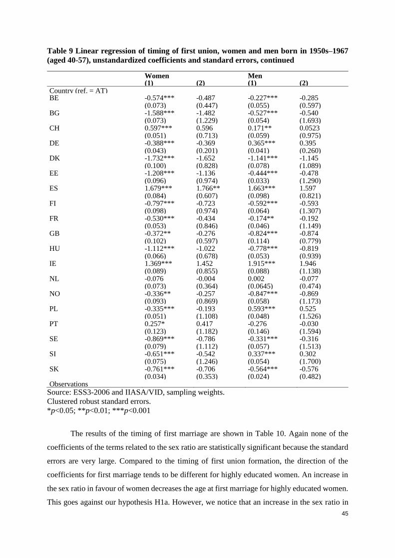
45

Table 9 Linear regression of timing of first union, women and men born in 1950s–1967

(aged 40-57), unstandardized coefficients and standard errors, continued

Women Men (1) (2) (1) (2) Country (ref. = AT) BE -0.574*** -0.487 -0.227*** -0.285 (0.073) (0.447) (0.055) (0.597) BG -1.588*** -1.482 -0.527*** -0.540 (0.073) (1.229) (0.054) (1.693) CH 0.597*** 0.596 0.171** 0.0523 (0.051) (0.713) (0.059) (0.975) DE -0.388*** -0.369 0.365*** 0.395 (0.043) (0.201) (0.041) (0.260) DK -1.732*** -1.652 -1.141*** -1.145 (0.100) (0.828) (0.078) (1.089) EE -1.208*** -1.136 -0.444*** -0.478 (0.096) (0.974) (0.033) (1.290) ES 1.679*** 1.766** 1.663*** 1.597 (0.084) (0.607) (0.098) (0.821) FI -0.797*** -0.723 -0.592*** -0.593 (0.098) (0.974) (0.064) (1.307) FR -0.530*** -0.434 -0.174** -0.192 (0.053) (0.846) (0.046) (1.149) GB -0.372** -0.276 -0.824*** -0.874 (0.102) (0.597) (0.114) (0.779) HU -1.112*** -1.022 -0.778*** -0.819 (0.066) (0.678) (0.053) (0.939) IE 1.369*** 1.452 1.915*** 1.946 (0.089) (0.855) (0.088) (1.138) NL -0.076 -0.004 0.002 -0.077 (0.073) (0.364) (0.0645) (0.474) NO -0.336** -0.257 -0.847*** -0.869 (0.093) (0.869) (0.058) (1.173) PL -0.335*** -0.193 0.593*** 0.525 (0.051) (1.108) (0.048) (1.526) PT 0.257* 0.417 -0.276 -0.030 (0.123) (1.182) (0.146) (1.594) SE -0.869*** -0.786 -0.331*** -0.316 (0.079) (1.112) (0.057) (1.513) SI -0.651*** -0.542 0.337*** 0.302 (0.075) (1.246) (0.054) (1.700) SK -0.761*** -0.706 -0.564*** -0.576 (0.034) (0.353) (0.024) (0.482) Observations

Source: ESS3-2006 and IIASA/VID, sampling weights.

Clustered robust standard errors.

*p<0.05; **p<0.01; ***p<0.001

The results of the timing of first marriage are shown in Table 10. Again none of the

coefficients of the terms related to the sex ratio are statistically significant because the standard

errors are very large. Compared to the timing of first union formation, the direction of the

coefficients for first marriage tends to be different for highly educated women. An increase in

the sex ratio in favour of women decreases the age at first marriage for highly educated women.

This goes against our hypothesis H1a. However, we notice that an increase in the sex ratio in

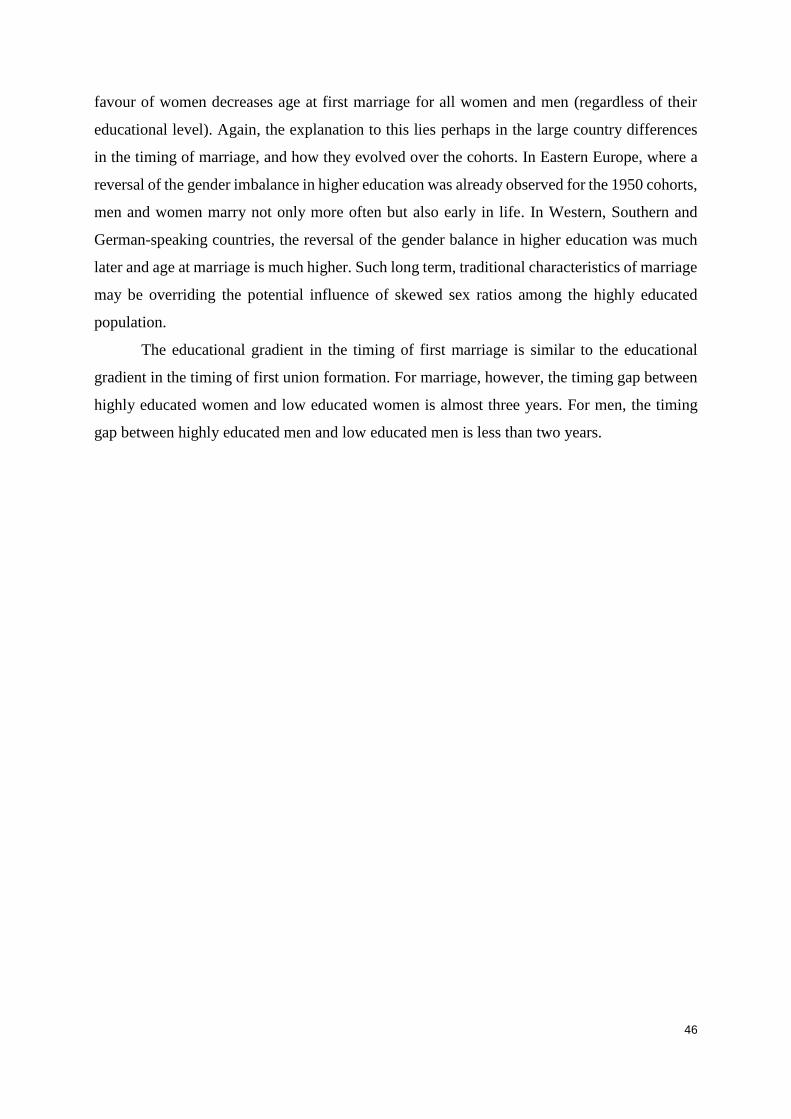
46

favour of women decreases age at first marriage for all women and men (regardless of their

educational level). Again, the explanation to this lies perhaps in the large country differences

in the timing of marriage, and how they evolved over the cohorts. In Eastern Europe, where a

reversal of the gender imbalance in higher education was already observed for the 1950 cohorts,

men and women marry not only more often but also early in life. In Western, Southern and

German-speaking countries, the reversal of the gender balance in higher education was much

later and age at marriage is much higher. Such long term, traditional characteristics of marriage

may be overriding the potential influence of skewed sex ratios among the highly educated

population.

The educational gradient in the timing of first marriage is similar to the educational

gradient in the timing of first union formation. For marriage, however, the timing gap between

highly educated women and low educated women is almost three years. For men, the timing

gap between highly educated men and low educated men is less than two years.

47

Table 10 Linear regression of timing of first marriage, women and men born in 1950s–

1967 (aged 40-57), unstandardized coefficients and standard errors

Women Men (1) (2) (1) (2) Education (ref. High) Low -2.859*** -2.855*** -1.633*** -1.610*** (0.350) (0.349) (0.228) (0.219) Medium -1.638*** -1.642*** -1.246*** -1.204*** (0.254) (0.258) (0.180) (0.181) Sex ratio -1.134 -3.169 (2.502) (2.696) Sex ratio*Low 0.273 0.591 (1.044) (0.755) Sex ratio*Medium -0.061 0.687 (0.656) (0.389) Age cohort -0.065* -0.079 -0.060 -0.094 (0.028) (0.049) (0.044) (0.049) In education 0.618 0.623 -0.712 -0.734 (0.385) (0.389) (0.792) (0.790) Cohort (ref. 1950-1954) 1955-1959 -0.050 -0.045 -0.001 0.006 (0.138) (0.138) (0.240) (0.238) 1960-1964 -0.099 -0.103 0.194 0.172 (0.276) (0.285) (0.508) (0.495) 1965-1969 0.153 0.147 0.579 0.549 (0.447) (0.461) (0.633) (0.637)

Constant 28.81*** 29.05*** 30.39*** 31.05***

(1.379) (1.723) (2.302) (2.223)

Observations 5131 5131 4049 4049

Source: ESS3-2006 and IIASA/VID, sampling weights.

Clustered robust standard errors.

*p<0.05; **p<0.01; ***p<0.001

(continued on next page)

48

Table 10 Linear regression of timing of first marriage, women and men born in 1950s–

1967 (aged 40-57), unstandardized coefficients and standard errors, continued

Women Men (1) (2) (1) (2) Country (ref. = AT) BE -1.039*** -0.740 -1.487*** -0.834 (0.090) (0.607) (0.060) (0.687) BG -2.969*** -2.154 -2.573*** -0.689 (0.089) (1.703) (0.047) (1.964) CH 1.489*** 1.039 0.966*** -0.224 (0.052) (0.981) (0.051) (1.117) DE -0.306*** -0.429 -0.025 -0.365 (0.046) (0.264) (0.036) (0.287) DK 1.503*** 2.044 1.983*** 3.237* (0.140) (1.136) (0.076) (1.264) EE -2.300*** -1.658 -2.630*** -1.166 (0.131) (1.331) (0.035) (1.503) ES 0.599*** 1.000 0.211 1.113 (0.081) (0.832) (0.111) (0.921) FI -0.036 0.605 -0.053 1.448 (0.128) (1.333) (0.060) (1.517) FR -0.878*** -0.317 -0.432*** 0.865 (0.059) (1.168) (0.049) (1.329) GB -1.103*** -0.715 -1.294*** -0.414 (0.119) (0.814) (0.124) (0.894) HU -2.378*** -1.924 -2.343*** -1.306 (0.079) (0.943) (0.049) (1.094) IE 0.148 0.694 0.276** 1.580 (0.117) (1.167) (0.093) (1.305) NL 0.252** 0.499 -0.181* 0.325 (0.072) (0.485) (0.066) (0.545) NO -0.155 0.419 -0.510*** 0.832 (0.124) (1.193) (0.050) (1.372) PL -1.731*** -0.983 -1.464*** 0.220 (0.055) (1.540) (0.041) (1.782) PT -1.030*** -0.309 -2.302*** -0.516 (0.125) (1.662) (0.158) (1.803) SE 2.074*** 2.805 2.544*** 4.266* (0.107) (1.532) (0.053) (1.754) SI -1.501*** -0.683 -1.019*** 0.883 (0.089) (1.725) (0.046) (1.968) SK -1.922*** -1.680** -2.518*** -1.979** (0.048) (0.491) (0.031) (0.572) Observations

Source: ESS3-2006 and IIASA/VID, sampling weights.

Clustered robust standard errors.

*p<0.05; **p<0.01; ***p<0.001

5 Conclusions

In recent decades a reversed gender gap in tertiary education has emerged in the majority of

European countries. Women have overtaken men in enrollment and completion of tertiary

education. As a result, there are more highly educated women than highly educated men

49

entering today’s mating markets. As people have education-specific partner preferences, we

expect that changes in the gender balance in higher education will influence the timing and

likelihood of partnership formation. Following Van Bavel (2012) we posit that the reversal of

the gender imbalance in higher education results in an education-specific mating squeeze for

highly educated women.

We have approached this question using two theoretical frameworks. Marital search

theory (Oppenheimer 1988) and sociocultural theory (Guttentag and Secord 1983) offer

explanations to how imbalances on the mating market may affect union formation rates. Based

on marital search theory, which rests on the simple rules of the supply of potential partners, we

expected lower rates of union formation for highly educated women (H1) and higher rates of

union formation for highly educated men (H2). In line with the sociocultural theory, which

holds that men react differently to sex ratio imbalances, it was expected that a higher number

of available partners discourages men from making a commitment to form a union.

Accordingly, we hypothesized that the reversal of the gender imbalance in higher education

lowers the rates of union formation for highly educated women and highly educated men (H3).

The study made use of the European Social Survey data, coming from the third survey

round in 2006. The study sample included respondents from 20 European countries, born

between 1950-1975. For some parts of the analysis we had to narrow the cohort range to 1950-

1967. The descriptive results confirmed that there is a substantial cross country heterogeneity

in the timing of entry into first union at different levels of education. In most countries, there

was some postponement of union formation across cohorts. Unlike with first union formation,

we saw substantial postponement of first marriage formation over cohorts and changes in the

proportions of people who ever got married. The observed differentials by country and cohort

are much larger for first marriages than for first union formation. For most countries, the

educational gradient of both first union formation and marriage was positive, but with less

consistent differences between the low and medium educated. Among the cohorts born in the

1950s, the gender imbalance in higher education had already turned to the advantage of women

in 11 countries of the 20 in our sample. For the cohorts born in 1975, the gender imbalance in

higher education had turned to the advantage of women in all countries expect Austria, The

Netherlands, Switzerland and Germany. We proceeded to test whether these changes at the

macro level had the hypothesized association with union formation rates at the micro level.

We analysed the association between the shifting gender balance in higher education

and the rates of first union formation by means of survival modelling. To further disentangle

the timing and quantum components in the transition rate models, linear and binary logistic

50

regressions were used to model separately the timing and the probability of first union

formation. The primary focus of the analysis was on entry into first union formation, either

marriage or non-marital cohabitation. In parallel, we selected only marriages and tested our

hypotheses on this subset of first unions. It was statistically not feasible to address unmarried

cohabitation separately due to low sample sizes.

The modelling results provided us with several insights to the association between the

gender balance in higher education and the rates of union formation. However, our data do not

lend full support to any of the hypotheses derived from the marriage squeeze perspective.

Sometimes, the point estimates were in line with what was hypothesized, but the standard errors

were too large to reach statistical significance, suggesting an imprecise estimation of the sex

ratio effects. Nevertheless, despite the weak statistical power of the estimated coefficients, the

direction of the associations lends some support to marital search theory when looking at the

timing of first union formation and to sociocultural theory when looking at the probability of

first union formation. In line with hypothesis H1, an increase in the number of highly educated

women relative to highly educated men was associated with a higher age at first union formation

and with a lower probability of first union formation among highly educated women. For highly

educated men, the presence of a relatively high number of highly educated women in the mating

market was associated with a lower age of first union formation (H2) but, on the other hand,

also with a lower probability of first union formation (H3). Again, these associations are

statistically not significant.

Similarly, we did not find support for our hypotheses about the association between the

shifting gender balance in higher education and the timing and likelihood of first marriage. In

general, changes in the gender balance in higher education in favour of women show a positive

effect on the timing and likelihood of entry into first marriage, but only the sex ratio effects for

the likelihood of first marriage of highly educated women are significant. Remarkably, the

results for highly educated women go in opposite direction as formulated in hypothesis H1. An

increase in the number of highly educated women relative to highly educated men was

associated with a higher probability to ever marry for highly educated women, and the

association was statistically significant. Results for highly educated men are supportive of

marital search theory but insignificant. A potential explanation for the positive effects of the

sex ratio on marriage could be the positive correlation between the sex ratio and marriage rates

across countries. The descriptive results showed high percentages of married and early marriage

for most of the Central and East European countries, where the gender balance in higher

education was already in favour of women in the 1950s birth cohorts, and lower rates of married

51

and late marriages for Western, Southern and German-speaking countries. While our models

include controls for country and cohorts (fixed effects), we did not include their interaction.

Our sex ratio measure, in contrast, is specific for combinations of country and cohort. So

perhaps our sex ratio measure was picking up cohort- and country-specific trends that may have

nothing to do with the sex ratio as such, but were just correlated with them. This remains to be

investigated in the future.

The results for the effect of education on the likelihood of first union formation and first

marriage corroborates earlier research findings by Dykstra and Poortman (2010) and Wiik and

Dommermuth (2014). For men, we found a positive educational gradient of the probability to

ever form a union and to ever marry. For women, we found an insignificant negative educational

gradient of the probability to ever form a union and a significant negative educational gradient

of the probability to ever marry. Furthermore, high educational attainment was positively

associated with the age at entry into first union and first marriage for both men and women.

The notion of the education-specific mating squeeze is based on the assumption of a

certain rigidity in partner preferences. The negative educational gradient of union and marriage

entry for women and the positive educational gradient for men suggest to some extent that

preferences have not changed. Nevertheless, we do not find evidence in this paper that highly

educated women suffer an education-specific mating squeeze. In an earlier paper, De Hauw,

Grow and Van Bavel (2015) observed that as the gender balance in higher education turned to

the advantage of women, highly educated women partner more often with less educated men,

suggesting that on average, in Europe, highly educated women tend to adjust their union

formation behaviour to the demographic reality on the mating market (see also Esteve et al.

2012), and that some modification in mating preferences are in place. Furthermore, as to the

timing and likelihood of union formation, we may speculate that mating market conditions set

by the shifting gender balance in higher education have a relatively weak influence compared

to other processes, such as those characterizing the Second Demographic Transition, for

example (Lesthaeghe 2010).

Still, our results suffer from imprecise estimation of sex ratio effects. Future work should

further attempt to improve on this. One way to try, if data were available, is to use panel model

approaches where country-specific populations are followed over time. Alternatively,

exogenous (random) shocks in the distribution by gender and education could be a useful

instrument to improve the estimation of the effect of the reversal of the gender balance in

education on union formation and marriage.

52

References

Akers, D.S. (1967). On Measuring the Marriage Squeeze. Demographic Research, 4(2): 907–

924.

Albrecht, C.M. and Albrecht, D.E. (2001). Sex Ratio and Family Structure in the

Nonmetropolitan United States. Sociological Inquiry, 71(1), 67–84.

Angrist, J. (2002). How Do Sex Ratios Affect Marriage and Labor Markets? Evidence from

America’s Second Generation. The Quarterly Journal of Economics, 117(3), 997–1038.

Becker, G.S. (1981). A Treatise on the Family. Cambridge: Harvard University Press.

Bernardi, F. (2001). Is it a Timing or a Probability Effect? Four Simulations and an Application

of Transition Rate Models to the Analysis of Unemployment Exit. Quality & Quantity, 35,

231–252.

Blossfeld, H.-P. (2009). Educational assortative marriage in comparative perspective. Annual

Review of Sociology, 35: 513–530.

Blossfeld, H.-P. and Huinink, J. (1991). Human Capital Investments or Norms of Role

Transition? How Women’s Schooling and Career Affect the Process of Family Formation.

Amercian Journal of Sociology, 97(1), 143–168.

Buss, D.M., Shackelford, T.K., Kirkpatrick, L.A. and Larsen, R.J. (2001). A Half Century of

Mate Preferences: The Cultural Evolution of Values. Journal of Marriage and Family,

63(2), 491–503.

Cheng, Y.A. (2014). Changing partner choice and marriage propensities by education in post-

industrial Taiwan, 2000-2010. Demographic Research, 31(33), 1007–1042.

Cready, C.M., Fossett, M.A. and Kiecolt, K.J. (1997). Mate Availability and African American

Family Structure in the U.S. Nonmetropolitan South. Journal of Marriage and Family,

59(1), 192–203.

Crowder, K.D. and Tolnay, S.E. (2000). A new marriage squeeze for black women: the role of

racial intermarriage by black men. Journal of Marriage and Family, 62(3), 792–807.

De Hauw, Y., Grow, A. and Van Bavel, J. (2015). The reversal of gender inequality in education

and assortative mating in Europe. Paper presented at the Population Association of

America Annual Meeting, April 30-May2, 2015, San Diego, CA.

De Hauw, Y., Piazza, F. and Van Bavel, J. (2014). Methodological report: The measurement of

education-specific mating squeeze. Families And Societies. Working paper series, (2014)

16.

53

Dykstra, P., and Poortman, A.-R. (2010). Economic resources and remaining single: trends over

time. European Sociological Review, 26(3), 277–290.

Diprete, T.A. and Buchmann, C. (2006). Gender-Specific Trends in the Value of Education and

the Emerging Gender Gap in College Completion. Demography, 43(1): 1–24.

Eeckhaut, M., Van de Putte, B., Gerris, J and Vermulst, A. (2011). Analysing the effect of

educational differences between partners: a methodological/theoretical comparison.

European Sociological Review, 27(4), 14.

Esteve, A., García-Román, J. and Permanyer, I. (2012). The gender-gap reversal in education

and its effect on union formation: the end of hypergamy? Population and Development

Review, 38(3): 535–546.

Fossett, M.A. and Kiecolt, K. (1991). A methodological review of the sex ratio: Alternatives

for comparative research. Journal of Marriage and the Family, 53(4), 941–957.

Glick P.C., Heer D.M., and Beresford J.C. (1963). Family formation and family composition:

trends and prospects, In: M.B. Sussman (ed.), Sourcebook on Marriage and the Family

2nd ed. (pp: 30-40). Houghton Mifflin: Boston.

Goldman, N., Westoff, C.F. and Hammerslough, C. (1984). Demography of the Marriage

Market in the United States. Population Index, 50(1), 5–25.

Goldstein, J.R. and Kenney C.T. (2001). Marriage delayed or marriage forgone? New cohort

forecasts of first marriage for U.S. women. American Sociological Review, 66(4): 506-

519.

Grow, A. and Van Bavel, J. (2015). Assortative Mating and the Reversal of Gender Inequality

in Education in Europe: An Agent-Based Model. PLoS ONE, (10)6.

Guttentag, M. and Secord, P.F. (1983). Too many women? The sex ratio question. Beverly Hills,

CA: Sage.

Guzzo, K.B. (2006). How do marriage market conditions affect entrance into cohabitation vs.

marriage? Social Science Research, 35(2), 332–355.

Hiekel, N., Liefbroer, A.C. and Poortman, A.-R. (2014). Understanding Diversity in the

Meaning of Cohabitation Across Europe. European Journal of Population, 30(5), 391–

410.

Jaccard, J. (2001). Interaction Effects in Logistic Regression. New York: Sage Publications.

K.C., S., Barakat, B., Goujon, A., Skirbekk, V., Sanderson, W.C. and Lutz, W. (2010).

Projection of Populations by Level of Educational Attainment, Age, and Sex for 120

Countries for 2005-2050. Demographic Research, 22: 383–472.

54

Kalmijn, M. (2013). The Educational Gradient in Marriage: A Comparison of 25 European

countries. Demography, 50(4): 1499–520.

Kravdal, O. (1999). Does marriage require a stronger economic underpinning than informal

cohabitation? Population Studies, 53(1), 63–80.

Lesthaeghe, R. (2010). The Unfolding Story of the Second Demographic Transition, Population

and Development Review, Vol. 36(2), 211-51.

Lichter, D.T., Leclere, F.B. and Mclaughlin, D.K. (1991). Local Marriage Markets and the

Marital Behavior of Black and White Women. American Journal of Sociology, 96(4), 843–

867.

Liefbroer, A.C. and Corijn, M. (1999). Who, what, where, and when? Specifying the impact of

educational attainment and labour force participation on family formation. European

Journal of Population, 15(1), 45–75.

Lloyd, K.M. and South, S.J. (1996). Contextual Ifluences on Young Men’s Transition to First

Marriage. Social Forces, 74(3), 1097–1119.

Lutz, W., Goujon, A., K.C., S. and Sanderson, W.C. (2007). Reconstruction of Populations By

Age, Sex and Level of Educational Attainment for 120 Countries for 1970-2000. Vienna

Yearbook of Population Research, 2007: 193–235.

Manning, W. D., Brown, S. L., and Payne, K. K. (2014). Two Decades of Stability and Change

in Age at First Union Formation. Journal of Marriage and Family, 76(2), 247–260.

Matysiak, A. (2009). Is Poland really ‘immune’ to the spread of cohabitation? Demographic

Research, 21(8), 215-234.

Muhsam, H.V. (1974). The Marriage Squeeze. Demography, 11(2), 291–299.

Oppenheimer, V.K. (1988). A theory of marriage timing. American Journal of Sociology, 94(3),

563–591.

Oppenheimer, V.K. (1997). Women’s employment and the gain to marriage: The specialization

and trading model of marriage. Annual Review of Sociology, 23, 431–453.

Park, H. and Smits, J. (2005). Educational Assortative Mating in South Korea: Trends 1930–

1998. Research in Social Stratification and Mobility, 23(5), 103–127.

Perelli-Harris, B. and Lyons-Amos, M. (2015). Changes in partnership patterns across the life

course: An examination of 14 countries in Europe and the United States. Demographic

Research, 33(1), 145–178.

Qian, Z. and Preston, S.H. (1993). Changes in American Marriage, 1972 to 1987: Availability

and Forces of Attraction by Age and Education. American Sociological Review, 58(4):

482.

55

Qian, Y. and Qian, Z. (2014). The gender divide in urban China: Singlehood and assortative

mating by age and education. Demographic Research, 31(45), 1337–1364.

Raymo, J. M. and Iwasawa, M. (2005). Marriage Market Mismatches in Japan: An Alternative

View of the Relationship between Women’s Education and Marriage. American

Sociological Review, 70(5), 801–822.

Rose, E. (2004). Education and Hypergamy in Marriage Markets. Washington, WA : Center

for Research on Families, University of Washington: 41.

Sassler, S. and Goldscheider, F. (2004). Revisiting Jane Austen’s Theory of Marriage Timing.

Journal of Family Issues, 25(2), 139–166.

Schmitt, D.P. (2005). Sociosexuality from Argentina to Zimbabwe: A 48 nation study of sex,

culture, and strategies of human mating. Behavioral and Brain Sciences, 28, 247–311.

Schoen, R. (1983). Measuring the tightness of the marriage squeeze. Demography, 20(1): 61–

78.

Schoen, R. and Kluegel, J.R. (1988). The Widening Gap in Black and White Marriage Rates:

The Impact of Population Composition and Differential Marriage Propensities.

American Sociological Review, 53(6), 895–907.

Schofer, E. and Meyer, J.W. (2005). The Worldwide Expansion of Higher Education in the

Twentieth Education Century. American Sociological Review, 70(6): 898–920.

Schwartz, C.R. (2013). Trends and Variation in Assortative Mating: Causes and Consequences.

Annual Review of Sociology: 1–41.

Schwartz, C.R. and Han, H. (2014). The Reversal of the Gender Gap in Education and Trends

in Marital Dissolution. American Sociological Review, 79(4): 605–629.

Schwartz, C.R. and Mare, R.D. (2005). Trends in Educational Assortative Marriage from 1940

to 2003. Demographic Research, 42(4): 621–646.

Sobotka, T. and Toulemon, L. (2008). Overview Chapter 4: Changing family and partnership

behaviour: Common trends and persistent diversity across Europe. Demographic

Research, 19(6), 85–138.

South, S.J. and Lloyd, K.M. (1992). Marriage Opportunities and Family Formation: Further

Implications of Imbalanced Sex Ratios. Journal of Marriage and the Family, 54(2): 440–

451.

Spanier, G.B.and Glick, P.C. (1980). Mate Selection Differentials Between Whites and Blacks

in the United States. Social Forces, 58(3), 707–725.

Sweeney, M.M. (2002). Two Decades of Family Change: The Shifting Economic Foundations

of Marriage. American Journal of Sociology, 67(1): 132–147.

56

Torr, B.M. (2011). The changing relationship between education and marriage in the United

States. Journal of Family History, 36: 483–503.

Uecker, J.E. and Regnerus, M.D. (2010). Bare Market: Campus Sex Ratios, Romantic

Relationships, and Sexual Behavior. The Sociological Quarterly, 51, 408–435.

Van Bavel, J. (2012). The reversal of gender inequality in education, union formation and

fertility in Europe. Vienna Yearbook of Population Research, 10: 127–154.

Vincent-Lancrin. (2008). The Reversal of Gender Inequalities in Higher Education: an Ongoing

Trend. In Higher Education to 2030: Demography (Vol. 1, pp. 265–298). Paris: OECD.

Warner, T.D., Manning, W.D., Giordano, P.C. and Longmore, M.A. (2011). Relationship

formation and stability in emerging adulthood: do sex ratios matter? Social Forces, 90(1),

269–295.

Wiik, K.A. (2009). You'd better wait! Socio-economic background and timing of first marriage

versus first cohabitation. European Sociological Review, 25: 139-153.

Wiik, K.A. and Dommermuth, L. (2014). Who Remains Unpartnered by Mid-Life in Norway?

Differentials by Gender and Education. Journal of Comparative Family Studies, XLV(3),

405–424.

Wilson, W.J. (1987). The Truly Disadvantaged. The Inner City, the Underclass, and Public

Policy. Chicago: The University of Chicago Press.