IMPLEMENTING LTL MODEL CHECKING WITH NET UNFOLDINGS

Helsinki University of Technology Laboratory for Theoretical Computer Science

Research Reports 68

Teknillisen korkeakoulun tietojenkasittelyteorian laboratorion tutkimusraportti 68

Espoo 2001 HUT-TCS-A68

IMPLEMENTING LTL MODEL CHECKING WITH

NET UNFOLDINGS

Javier Esparza and Keijo Heljanko

AB TEKNILLINEN KORKEAKOULUTEKNISKA HÖGSKOLANHELSINKI UNIVERSITY OF TECHNOLOGYTECHNISCHE UNIVERSITÄT HELSINKIUNIVERSITE DE TECHNOLOGIE D’HELSINKI

Helsinki University of Technology Laboratory for Theoretical Computer Science

Research Reports 68

Teknillisen korkeakoulun tietojenkasittelyteorian laboratorion tutkimusraportti 68

Espoo 2001 HUT-TCS-A68

IMPLEMENTING LTL MODEL CHECKING WITH

NET UNFOLDINGS

Javier Esparza and Keijo Heljanko

Helsinki University of Technology

Department of Computer Science and Engineering

Laboratory for Theoretical Computer Science

Teknillinen korkeakoulu

Tietotekniikan osasto

Tietojenkasittelyteorian laboratorio

Distribution:

Helsinki University of Technology

Laboratory for Theoretical Computer Science

P.O.Box 5400

FIN-02015 HUT

Tel. +358-0-451 1

Fax. +358-0-451 3369

E-mail: [email protected]

©c Javier Esparza and Keijo Heljanko

ISBN 951-22-5390-9

ISSN 1457-7615

Picaset Oy

Helsinki 2001

ABSTRACT: We report on an implementation of the unfolding approach tomodel-checking LTL-X recently presented by the authors. Contrary to thatwork, we consider an state-based version of LTL-X, which is more used inpractice. We improve on the checking algorithm; the new version allows toreuse code much more efficiently. We present results on a set of case studies.

KEYWORDS: Net unfoldings, model checking, tableau systems, Petri nets,LTL

Contents

1 Introduction 1

2 Petri nets 1

3 Automata Theoretic Approach to Model Checking LTL 3

4 Basic definitions on unfoldings 7

5 Tableau System 10

6 Generating the Tableau 11

7 Experimental Results 16

8 Conclusions 18

9 Appendix A - Proofs of Theorems 22

1 INTRODUCTION

Unfoldings [14, 6, 5] are a partial-order approach to the automatic verifica-tion of concurrent and distributed systems, in which partial-order semanticsis used to generate a compact representation of the state space. For systemsexhibiting a high degree of concurrency, this representation can be exponen-tially more succinct than the explicit enumeration of all states or the symbolicrepresentation in terms of a BDD, thus providing a very good solution to thestate-explosion problem.

Unfolding-based model-checking techniques for LTL without the next op-erator (called LTL-X in the sequel) were first proposed in [22]. A new algo-rithm with better complexity bounds was introduced in [3], in the shape of atableau system. The approach is based on the automata-theoretic approachto model-checking (see for instance [20]), consisting of the following well-known three steps: (1) translate the negation of the formula to be checkedinto a Büchi automaton; (2) synchronize the system and the Büchi automa-ton in an adequate way to yield a composed system, and (3) check emptinessof the language of the composed system, where language is again defined ina suitable way.

In [3] we used an action-based version of LTL-X having an operator φ1Uaφ2

for each action a; φ1Uaφ2 holds if φ1 holds until action a occurs, and imme-

diately after φ2 holds. Step (2) is very simple for this logic, which allowed usto concentrate on step (3), the most novel contribution of [3]. However, thestate-based version of LTL-X is more used in practice. The first contributionof this paper is a solution to step (2) for this case, which turns out to be quitedelicate.

The second contribution of this paper concerns step (3). In [3] we pre-sented a two-phase solution; the first phase requires to construct one tableau,while the second phase requires to construct a possibly large set of tableaux.We propose here a more elegant solution which, loosely speaking, allows tomerge all the tableaux of [3] into one while keeping the rules for the tableauconstruction simple and easy to implement.

The third contribution is an implementation using the smodels NP-solver[18], and a report on a set of case studies.

The paper is structured as follows. Section 2 contains basic definitions onPetri nets, which we use as system model. Section 3 describes step (2) abovefor the state-based version of LTL-X. Readers wishing to skip this sectionneed only read (and believe the proof of) Theorem 1. Section 4 presentssome basic definitions about the unfolding method. Section 5 describes thenew tableau system for (3), and shows its correctness. Section 6 discusses thetableau generation together with some optimizations. Section 7 reports onthe implementation and case studies, and Section 8 contains conclusions.

2 PETRI NETS

A net is a triple (P, T, F ), where P and T are disjoint sets of places andtransitions, respectively, and F is a function (P × T ) ∪ (T × P ) → {0, 1}.Places and transitions are generically called nodes. If F (x, y) = 1 then we

2 PETRI NETS 1

say that there is an arc from x to y. The preset of a node x, denoted by •x, isthe set {y ∈ P ∪ T | F (y, x) = 1}. The postset of x, denoted by x•, is theset {y ∈ P ∪ T | F (x, y) = 1}. In this paper we consider only nets in whichevery transition has a nonempty preset and a nonempty postset.

A marking of a net (P, T, F ) is a mapping P → IN (where IN denotes thenatural numbers including 0). We identify a marking M with the multisetcontaining M(p) copies of p for every p ∈ P . For instance, if P = {p1, p2}and M(p1) = 1, M(p2) = 2, we write M = {p1, p2, p2}.

A marking M enables a transition t if it marks each place p ∈ •t with atoken, i.e. if M(p) > 0 for each p ∈ •t. If t is enabled at M , then it can fire oroccur, and its occurrence leads to a new marking M ′, obtained by removinga token from each place in the preset of t, and adding a token to each placein its postset; formally, M ′(p) = M(p) − F (p, t) + F (t, p) for every place p.

For each transition t the relationt

−−−→ is defined as follows: Mt

−−−→M ′ if tis enabled at M and its occurrence leads to M ′.

A 4-tuple Σ = (P, T, F, M0) is a net system if (P, T, F ) is a net and M0

is a marking of (P, T, F ) (called the initial marking of Σ). A sequence oftransitions σ = t1t2 . . . tn is an occurrence sequence if there exist markingsM1, M2, . . . , Mn such that

M0t1−−−→M1

t2−−−→ . . .Mn−1tn−−−−→Mn

Mn is the marking reached by the occurrence of σ, which is also denoted by

M0σ

−−−→Mn. A marking M is a reachable marking if there exists an occur-

rence sequence σ such that M0σ

−−−→M . An execution is an infinite occur-rence sequence starting from the initial marking. The reachability graph ofa net system Σ is the labelled graph having the reachable markings of Σ as

nodes, and thet

−−−→ relations (more precisely, their restriction to the set ofreachable markings) as edges. In this work we only consider net systems withfinite reachability graphs.

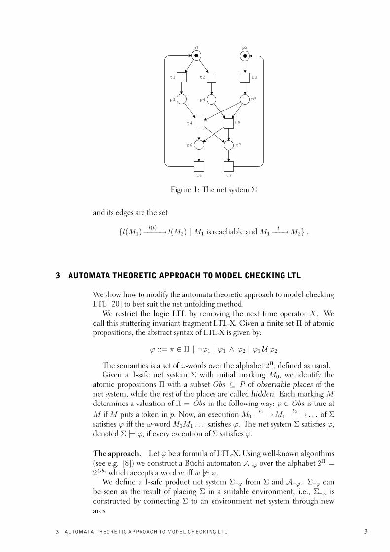
A marking M of a net is n-safe if M(p) ≤ n for every place p. A net systemΣ is n-safe if all its reachable markings are n-safe. Fig. 1 shows a 1-safe netsystem.

Labelled nets. Let L be an alphabet. A labelled net is a pair (N, l) (alsorepresented as a 4-tuple (P, T, F, l)), where N is a net and l : P ∪ T → Lis a labelling function. Notice that different nodes of the net can carry thesame label. We extend l to multisets of P ∪ T in the obvious way.

For each label a ∈ L we define the relationa

−−−→ between markings as

follows: Ma

−−−→M ′ if Mt

−−−→M ′ for some transition t such that l(t) = a.For a finite sequence w = a1a2 . . . an ∈ L∗, M

w−−−→M ′ denotes that for

some reachable markings M1, M2, . . . , Mn−1 of the net system the relation

Ma1−−−−→M1

a2−−−−→M2 . . .Mn−1an−−−−→M ′ holds. For an infinite sequence

w = a1a2 . . . ∈ Lω, Mw

−−−→ denotes that Ma1−−−−→M1

a2−−−−→ M2 . . .holds for some reachable markings M1, M2, . . . .

The reachability graph of a labelled net system (N, l, M0) is obtained byapplying l to the reachability graph of (N, M0). In other words, its nodes arethe set

{l(M) | M is a reachable marking}

2 2 PETRI NETS

p1 p2

p3 p4 p5

p6

t1 t2 t3

t4 t5

t6

p7

t7

Figure 1: The net system Σ

and its edges are the set

{l(M1)l(t)

−−−−→ l(M2) | M1 is reachable and M1t

−−−→M2} .

3 AUTOMATA THEORETIC APPROACH TO MODEL CHECKING LTL

We show how to modify the automata theoretic approach to model checkingLTL [20] to best suit the net unfolding method.

We restrict the logic LTL by removing the next time operator X . Wecall this stuttering invariant fragment LTL-X. Given a finite set Π of atomicpropositions, the abstract syntax of LTL-X is given by:

ϕ ::= π ∈ Π | ¬ϕ1 | ϕ1 ∧ ϕ2 | ϕ1 U ϕ2

The semantics is a set of ω-words over the alphabet 2Π, defined as usual.Given a 1-safe net system Σ with initial marking M0, we identify the

atomic propositions Π with a subset Obs ⊆ P of observable places of thenet system, while the rest of the places are called hidden. Each marking Mdetermines a valuation of Π = Obs in the following way: p ∈ Obs is true at

M if M puts a token in p. Now, an execution M0t1−−−→M1

t2−−−→ . . . of Σsatisfies ϕ iff the ω-word M0M1 . . . satisfies ϕ. The net system Σ satisfies ϕ,denoted Σ |= ϕ, if every execution of Σ satisfies ϕ.

The approach. Let ϕ be a formula of LTL-X. Using well-known algorithms(see e.g. [8]) we construct a Büchi automaton A¬ϕ over the alphabet 2Π =2Obs which accepts a word w iff w 6|= ϕ.

We define a 1-safe product net system Σ¬ϕ from Σ and A¬ϕ. Σ¬ϕ canbe seen as the result of placing Σ in a suitable environment, i.e., Σ¬ϕ isconstructed by connecting Σ to an environment net system through newarcs.

3 AUTOMATA THEORETIC APPROACH TO MODEL CHECKING LTL 3

It is easy to construct a product net system with a distinguished set of tran-sitions I such that Σ violates ϕ iff some execution of the product fires sometransition of I infinitely often. We call such an execution an illegal ω-trace.However, this product synchronizes A¬ϕ with Σ on all transitions, which ef-fectively disables all concurrency present in Σ. Since the unfolding approachexploits the concurrency of Σ in order to generate a compact representationof the state space, this product is not suitable, and so we propose a new one.

We define the set V of visible transitions of Σ as the set of transitions whichchange the marking of some observable place of Σ. Only these transitionswill synchronize with the automaton. So, for instance, in order to check aproperty of the form 2(p → 3q), where p and q are places, we will onlysynchronize with the transitions removing or adding tokens to p and q. Thisapproach is similar but not identical to Valmari’s tester approach describedin [19]. (In fact, a subtle point in Valmari’s construction makes its directimplementation unsuitable for checking state based LTL-X.)

The price to pay for this nicer synchronization is the need to check notonly for illegal ω-traces, but also for so-called illegal livelocks. The new prod-uct contains a new distinguished set of transitions L (for livelock). An il-legal livelock is an execution of the form σ1tσ2 such that t ∈ L and σ2

does not contain any visible transition. For convenience we use the nota-

tion M0σ

−−−→Mτ

−−−→ to denote this, and implicitly require that σ = σ1twith t ∈ L and that τ is an infinite sequence which only contains invisibletransitions.

In the rest of the section we define Σ¬ϕ. Readers only interested in thedefinition of the tableau system for LTL model-checking can safely skip it.Only the following theorem, which is proved hand in hand with the defini-tion, is necessary for it. Property (b) is what we win by our new approach:The environment only interferes with the visible transitions of Σ.

Theorem 1 Let Σ be a 1-safe net system whose reachable markings are pair-wise incomparable with respect to set inclusion.1 Let ϕ be an LTL-X formulaover the observable places of Σ. It is possible to construct a net system Σ¬ϕ

satisfying the following properties:

(a) Σ |= ϕ iff Σ¬ϕ has neither illegal ω-traces nor illegal livelocks.

(b) The input and output places of the invisible transitions are the same inΣ and Σ¬ϕ.

Construction of Σ¬ϕ We describe the synchronization Σ¬ϕ of Σ and A¬ϕ

in a semiformal but hopefully precise way. Let us start with two preliminar-ies. First, we identify the Büchi automaton A¬ϕ with a net system havinga place for each state q, with only the initial state q0 having a token, and anet transition for each transition (q, x, q′); the input and output places of thetransition are q and q′, respectively; we keep A¬ϕ, q and (q, x, q′) as namesfor the net representation, the place and the transition. Second, we split theexecutions of Σ that violate ϕ into two classes: executions of type I, which

1This condition is purely technical. Any 1-safe net system can be easily transformed intoan equivalent one satisfying it by adding some extra places and arcs; moreover, the conditioncan be removed at the price of a less nice theory.

4 3 AUTOMATA THEORETIC APPROACH TO MODEL CHECKING LTL

contain infinitely many occurrences of visible transitions, and executions oftype II, which only contain finitely many. We will deal with these two typesseparately.

Σ¬ϕ is constructed in several steps:

(1) Put Σ and (the net representation of) A¬ϕ side by side.

(2) For each observable place p add a complementary place (see [17]) p toΣ.p is marked iff p is not, and so checking that proposition p does nothold is equivalent to checking that the place p has a token. A set x ⊆ Πcan now be seen as a conjunction of literals, where p ∈ x is used todenote p ∈ (Π \ x).

(3) Add new arcs to each transition (q, x, q′) of A¬ϕ so that it “observes”the places in x.This means that for each literal p (p) in x we add an arc from p (p) to(q, x, q′) and an arc from (q, x, q′) to p (p). The transition (q, x, q′) canonly be enabled by markings of Σ satisfying all literals in x.

(4) Add a scheduler guaranteeing that:

– Initially A¬ϕ can make a move, and all visible moves (i.e., thefirings of visible transitions) of Σ are disabled.

– After a move of A¬ϕ, only Σ can make a move.

– After Σ makes a visible move, A¬ϕ can make a move and untilthat happens all visible moves of Σ are disabled.

This is achieved by introducing two scheduler places sf and ss [22].The intuition behind these places is that when sf (ss) has a token it isthe turn of the Büchi automaton (the system Σ) to make a move. Inparticular, visible transitions transfer a token from ss to sf , and Büchitransitions from sf to ss. Because the Büchi automaton needs to ob-serve the initial marking of Σ, we initially put one token in sf and notokens on ss.

(5) Let I be a subset of transitions defined as follows. A transition belongsto I iff its postset contains a final state of A¬ϕ.

Observe that since only moves of A¬ϕ and visible moves of Σ are scheduled,invisible moves can still be concurrently executed.

Let Σ′

¬ϕ be the net system we have constructed so far. The following is animmediate consequence of the definitions:

Σ has an execution of type I if and only if Σ′

¬ϕ has an illegal ω-trace.

We now extend the construction in order to deal with executions of type II.Let σ be a type II execution of Σ. Take the sequence of markings reachedalong the execution of σ, and project it onto the observable places. Since σonly contains finitely many occurrences of visible transitions, the result is a

3 AUTOMATA THEORETIC APPROACH TO MODEL CHECKING LTL 5

sequence of the form O00O

10 . . . Oj

0O01O

11 . . . Ok

1O02 . . . O0

n(On)ω. (The moves

from Oi to Oi+1 are caused by the firing of visible transitions.)We can split σ into two parts: a finite prefix σ1 ending with the last occur-

rence of a visible transition (σ1 is empty if there are no visible transitions),and an infinite suffix σ2 containing only invisible transitions. Clearly, theprojection onto the observable places of the marking reached by the execu-tion of σ1 is On

Since LTL-X is closed under stuttering, A¬ϕ has an accepting run

r = q0O0−−−−→ q1

O1−−−−→ . . .On−1

−−−−−→ qnOn−−−−→ qn+1

On−−−−→ qn+2 . . .

where the notation qO

−−−→ q′ means that a transition (q, x, q′) is taken suchthat the literals of x are true at the valuation given by O. We split this run

into two parts: a finite prefix r1 = q0O0−−−−→ q1 . . . qn−1

On−1

−−−−−→ qn and an

infinite suffix r2 = qnOn−−−−→ qn+1

On−−−−→ qn+2 . . . .In the net system representation of A¬ϕ, r1 and r2 correspond to occur-

rence sequences. By construction, the “interleaving” of r1 and σ1 yields anoccurrence sequence τ1 of Σ′

¬ϕ.Observe that reachable markings of Σ′

¬ϕ are of the form (q, s, O, H), mean-ing that they consist of a token on a state q of A¬ϕ, a token on one of theplaces of the scheduler (i.e., s ∈ {ss, sf}), a marking O of the observableplaces, and a marking H of the hidden places. Let (qn, sf , On, H) be themarking of Σ′

¬ϕ reached after executing τ1. (We have s = sf because the lasttransition of σ1 is visible.) The following property holds: With qn as initialstate, the Büchi automaton A¬ϕ accepts the sequence Oω

n . We call any pair(q, O) satisfying this property a checkpoint and define Σ¬ϕ as follows:

(6) For each checkpoint (q, O) and for each reachable marking (q, sf , O, H)of Σ′

¬ϕ, add a new transition having all the places marked at (q, sf , O, H)as preset, and all the places marked at O and H as postset. Let L (forlivelocks) be this set of transitions.

The reader has possibly observed that the set L can be very large, becausethere can be many hidden markings H for a given marking O (exponentiallymany in the size of Σ). Apparently, this makes Σ¬ϕ unsuitable for model-checking. In Sect. 6 we show that this is not the case, because Σ¬ϕ need notbe explicitly constructed.

Observe that after firing a L-transition no visible transition can occur any-more, because all visible transitions need a token on ss for firing. We prove:

Σ has an execution of type II if and only if Σ¬ϕ has an illegal livelock.

For the only if direction, assume first that σ is a type II execution of Σ. Letτ1 be the occurrence sequence of Σ¬ϕ defined above (as the “interleaving” ofthe prefix σ1 of σ and the prefix r1 of r). Further, let (qn, sf , On, H) be themarking reached after the execution of τ1, and let t be the transition addedin (6) for this marking. Define ρ1 = τ1 and ρ2 = σ2. It is easy to show thatρ1tρ2 is an execution of Σ¬ϕ and so an illegal livelock. For the if direction,let ρ1tρ2 be an illegal livelock of Σ¬ϕ, where t is an L-transition. After the

6 3 AUTOMATA THEORETIC APPROACH TO MODEL CHECKING LTL

firing of t there are no tokens in the places of the scheduler, and so no visibletransition can occur again; hence, no visible transition of Σ occurs in ρ2. Letσ1 and σ2 be the projections of ρ1 and ρ2 onto the transitions of Σ. It is easyto see that σ = σ1σ2 is an execution of Σ. Since σ2 does not contain anyvisible transition, σ is an execution of type II.

4 BASIC DEFINITIONS ON UNFOLDINGS

In this section we briefly introduce the definitions we needed to describe theunfolding approach. More details can be found in [6].

Occurrence nets. Given two nodes x and y of a net, we say that x is causallyrelated to y, denoted by x ≤ y, if there is a (possibly empty) path of arrowsfrom x to y. We say that x and y are in conflict, denoted by x#y, if there is aplace z, different from x and y, from which one can reach x and y, exiting zby different arrows. Finally, we say that x and y are concurrent, denoted byx co y, if neither x < y nor y < x nor x#y hold. A co-set is a set of nodes Xsuch that x co y for every x, y ∈ X . Occurrence nets are those satisfying thefollowing three properties: the net, seen as a directed graph, has no cycles;every place has at most one input transition; and, no node is in self-conflict,i.e., x#x holds for no x. A place of an occurrence net is minimal if it has noinput transitions. The net of Fig. 2 is an infinite occurrence net with minimalplaces a, b. The default initial marking of an occurrence net puts one tokenon each minimal place an none in the rest.

Branching processes. We associate to Σ a set of labelled occurrence nets,called the branching processes of Σ. To avoid confusions, we call the placesand transitions of branching processes conditions and events, respectively.The conditions and events of branching processes are labelled with placesand transitions of Σ, respectively. The conditions and events of the branch-ing processes are subsets from two sets B and E , inductively defined as thesmallest sets satisfying the following conditions:

• ⊥ ∈ E , where ⊥ is an special symbol;

• if e ∈ E , then (p, e) ∈ B for every p ∈ P ;

• if ∅ ⊂ X ⊆ B, then (t, X) ∈ E for every t ∈ T .

In our definitions of branching process (see below) we make consistentuse of these names: The label of a condition (p, e) is p, and its unique inputevent is e. Conditions (p,⊥) have no input event, i.e., the special symbol⊥ is used for the minimal places of the occurrence net. Similarly, the labelof an event (t, X) is t, and its set of input conditions is X . The advantageof this scheme is that a branching process is completely determined by itssets of conditions and events. We make use of this and represent a branchingprocess as a pair (B, E).

Definition 1 The set of finite branching processes of a net system Σ with theinitial marking M0 = {p1, . . . , pn} is inductively defined as follows:

4 BASIC DEFINITIONS ON UNFOLDINGS 7

• ({(p1,⊥), . . . , (pn,⊥)}, ∅) is a branching process of Σ.

• If (B, E) is a branching process of Σ, t ∈ T , and X ⊆ B is a co-set labelled by •t, then ( B ∪ {(p, e) | p ∈ t•} , E ∪ {e} ) is also abranching process of Σ, where e = (t, X). If e /∈ E, then e is called apossible extension of (B, E).

The set of branching processes of Σ is obtained by declaring that the unionof any finite or infinite set of branching processes is also a branching process,where union of branching processes is defined componentwise on conditionsand events. Since branching processes are closed under union, there is aunique maximal branching process, called the unfolding of Σ. The unfoldingof our running example is an infinite occurrence net. Figure 2 shows aninitial part. Events and conditions have been assigned identificators that willbe used in the examples. For instance, the event (t1, {(p1,⊥)}) is assignedthe identificator 1.

p1

p1 p1

p2

p2 p2

p3

p3 p3

p4

p4 p4

p5

p5 p5

p6 p6

p6 p6p6 p6

t1

t1 t1

t2

t2 t2

t3

t3 t3

t4

t4 t4

t5

t5 t5

t6 t6

p7 p7

p7 p7p7 p7

t7 t7

.

.

.

.

.

.

.

.

.

.

.

.

.

.

.

.

.

.

.

.

.

.

.

.

1 2 3

4 5

6 7 8 9

10 11 12 13 14 15

16 17 18 19

c d e

f g h i

j k l m

n o p q r s

t u v w x y z a’

a b

Figure 2: The unfolding of Σ

We take as partial order semantics of Σ its unfolding. This is justified, be-cause it can be easily shown the reachability graphs of Σ and of its unfoldingcoincide. (Notice that the unfolding of Σ is a labelled net system, and so itsreachability graph is defined as the image under the labelling function of thereachability graph of the unlabelled system.)

8 4 BASIC DEFINITIONS ON UNFOLDINGS

Configurations. A configuration of an occurrence net is a set of events Csatisfying the two following properties: C is causally closed, i.e., if e ∈ Cand e′ < e then e′ ∈ C, and C is conflict-free, i.e., no two events of Care in conflict. Given an event e, we call [e] = {e′ ∈ E | e′ ≤ e} thelocal configuration of e. Let Min denote the set of minimal places of thebranching process. A configuration C of the branching process is associatedwith a marking of Σ denoted by Mark(C) = l((Min ∪ C•) \ •C). Thecorresponding set of conditions associated with a configuration is called acut, and it is defined as Cut(C) = ((Min ∪ C•) \ •C).

In Fig. 2, {1, 3, 4, 6} is a configuration, and {1, 4} (not causally closed)or {1, 2} (not conflict-free) are not. A set of events is a configuration if andonly if there is one or more firing sequences of the occurrence net (fromthe default initial marking) containing each event from the set exactly once,and no further events. These firing sequences are called linearisations. Theconfiguration {1, 3, 4, 6} has two linearisations, namely 1 3 4 6 and 3 1 4 6.All linearisations lead to the same reachable marking. For example, the twosequences above lead to the marking {p1, p7}. By applying the labellingfunction to a linearisation we obtain a firing sequence of Σ. Abusing oflanguage, we also call this firing sequence a linearisation. In our example weobtain t1t3t4t6 and t3t1t4t6 as linearisations.

Given a configuration C, we denote by ↑C the set of events of the un-folding {e | e 6∈ C ∧ ∀e′ ∈ C : ¬(e#e′)}. Intuitively, ↑C corresponds tothe behavior of Σ from the marking reached after executing any of the lin-earisations of C. We call ↑C the continuation after C of the unfolding of Σ.If C1 and C2 are two finite configurations leading to the same marking, i.e.Mark(C1) = M = Mark(C2), then ↑C1 and ↑C2 are isomorphic, i.e., thereis a bijection between them which preserves the labelling of events and thecausal, conflict, and concurrency relations (see [6]).

Adequate orders. To implement a net unfolding algorithm we need thenotion of adequate order on configurations [6]. Given a configuration C ofthe unfolding of Σ, we denote by C ⊕ E the set C ∪ E, under the conditionthat C ∪ E is a configuration satisfying C ∩ E = ∅. We say that C ⊕ E isan extension of C. Now, let C1 and C2 be two finite configurations leadingto the same marking. Then ↑C1 and ↑C2 are isomorphic. This isomorphism,say f , induces a mapping from the extensions of C1 onto the extensions ofC2; the image of C1 ⊕ E under this mapping is C2 ⊕ f(E).

Definition 2 A partial order ≺ on the finite configurations of the unfoldingof a net system is an adequate order if:

• ≺ is well-founded,

• C1 ⊂ C2 implies C1 ≺ C2, and

• ≺ is preserved by finite extensions; if C1 ≺ C2 and Mark(C1) =Mark(C2), then the isomorphism f from above satisfies C1 ⊕ E ≺C2 ⊕ f(E) for all finite extensions C1 ⊕ E of C1.

Total adequate orders for 1-safe Petri nets and for synchronous products oftransition systems have been presented in [6, 5].

4 BASIC DEFINITIONS ON UNFOLDINGS 9

5 TABLEAU SYSTEM

We showed in Section 3 that the model checking problem for LTL-X canbe solved by checking the existence of illegal ω-traces and illegal livelocks inΣ¬ϕ. In [3] these problems are solved using tableau techniques. A branchingprocess can be seen as a “distributed” tableau, in which conditions are “facts”and events represent “inferences”. For two conditions b and b′, b co b′ modelsthat the facts represented by b and b′ can be simultaneously true. A tableau isconstructed by adding new events (inferences) one by one following an ade-quate order; some events are declared as “terminals”, and the construction ofthe tableau terminates when no new event can be added having no terminalsamong its predecessors.

The tableau systems of [3] require to construct a possibly large set ofbranching processes. Here we present a new tableau system consisting ofone single branching process.2

An Adequate Order for LTL. We simplify the implementation of the tableausystem by selecting a special adequate order. We use≺ to denote the total ad-equate order defined for 1-safe Petri nets in [6]. We call an event correspond-ing to an L-transition an L-event. We define for a set of events C the functionbefore L-event as BL(C) = {e ∈ C | [e] \ {e} contains no L-events}. Thefunction after L-event is defined correspondingly as AL(C) = (C \ BL(C)).We can now define our new adequate order.

Definition 3 Let C1 and C2 be two finite configurations of the unfolding ofthe product net system Σ¬ϕ. C1 ≺LTL C2 holds if

• BL(C1) ≺ BL(C2), or

• BL(C1) = BL(C2) and C1 ≺ C2.

The adequate order ≺LTL is application specific in the sense that it isnot an adequate order for an arbitrary net system Σ, but needs some specialproperties of the net system Σ¬ϕ. We have the following result.

Theorem 2 The order ≺LTL is a total adequate order for finite configura-tions of the unfolding of Σ¬ϕ.

Proof:See Appendix A for the proof. ut

New Tableau System. We first divide the unfolding of Σ¬ϕ into two disjointsets of events. Intuitively, the first set is used for the ω-trace detection part,and the second for the illegal livelock detection part. We define part-I to bethe set of events e such that [e] does not contain an L-event and part-II as theset of events which are not in part-I.

2For the reader familiar with [3]: the L-transitions in the net system Σ¬ϕ act as glue

to connect a set of branching processes (the tableau components of [3]) together into onelarger tableau.

10 5 TABLEAU SYSTEM

Definition 4 An event e of the unfolding Σ¬ϕ is a terminal, if there existsanother event e′ such that Mark([e′]) = Mark([e]), [e′] ≺LTL [e], and one ofthe following two mutually exclusive cases holds:

(I) e ∈ part-I, and either

(a) e′ < e, or

(b) ¬(e′ < e) and #I [e′] ≥ #I [e], where #IC denotes the number

of I -events in C.

(II) e ∈ part-II, and either

(a) BL([e′]) ≺LTL BL([e]), or

(b) BL([e′]) = BL([e]) and ¬(e′#e), or

(c) BL([e′]) = BL([e]), e′#e, and |[e′]| ≥ |[e]|.

A tableau T is a branching process (B, E) of Σ¬ϕ such that for every possibleextension e of (B, E) at least one of the immediate predecessors of e is aterminal. A terminal is successful if it is type (I)(a) and [e]\ [e′] contains an I -event, or it is of type (II)(b). All other terminals are unsuccessful. A tableau Tis successful if it contains a successful terminal, otherwise it is unsuccessful.

Loosely speaking, a tableau is a branching process which cannot be ex-tended without adding a causal successor to a terminal.

We have the following result:

Theorem 3 Let T be a tableau for Σ¬ϕ.

• Σ¬ϕ has an illegal ω-trace iff T has a successful terminal of type I.

• Σ¬ϕ has an illegal livelock iff T has a successful terminal of type II.

• T contains at most K2 non-terminal events, where K is the number ofreachable markings of Σ¬ϕ.

Proof:See Appendix A for the proof. ut

6 GENERATING THE TABLEAU

We describe an implementation of the tableau system of Sect. 5. The maingoal is to keep the tableau generation as similar as possible to a conventionalprefix generation algorithm [6]. In this way any prefix generation algorithmcan be easily adapted to also perform LTL model checking.

The tableau generation algorithm (Algorithm 1) is almost identical to themain routine of a prefix generation algorithm. The changes are: an addi-tional block of code devoted to generating the L-events dynamically; a differ-ent but easy to implement adequate order; a new cut-off detection subrou-tine. The main feature of the implementation is the efficient handling ofL-transitions, which we discuss next.

6 GENERATING THE TABLEAU 11

Generating the L-transitions Dynamically. Recall that in the synchroniza-tion Σ¬ϕ we can for each Büchi state q have as many L-transitions as there arereachable markings of the form (q, sf , O, H) in the net system Σ¬ϕ. Clearlywe can not explicitly generate them all due to efficiency reasons. Instead wegenerate a net system Σs

¬ϕ (s stands for static) in which this set of L-transitions(added by step (6) of the synchronization procedure in Section 3) is replacedby:

(6’) Add for each Büchi transition t = (q, x, q′) in the net system Σ′

¬ϕ (i.e.,the synchronization after steps (1)-(5) as defined in Sect. 3) a new tran-sition t′. The preset of t′ is equivalent to the preset of t and the postsetof t′ is empty. Let L (for livelocks) be this set of transitions.

We can now dynamically generate any of the (enabled) L-transitions ofΣ¬ϕ. Namely, for a transition t corresponding to a reachable marking M =(q, sf , O, H) to be enabled in Σ¬ϕ, a transition t′ (for some (q, x, q′)) must beenabled in Σs

¬ϕ and the Büchi automaton must accept Oω when q is givenas the initial state. Loosely speaking we test the first label of the sequenceusing the transition t′, and if this test succeeds we check whether O can beinfinitely stuttered. (Using this construction it is easy to implement “no-carevalues” for selected atomic propositions by leaving them out of the preset oft′.) Now generating the postset of t from M is trivial.

Optimizations in Dynamic Creation. We can thus dynamically generateL-transitions for each reachable marking M as required. However, we cando better by using the net unfolding method. The main idea is to generatethe unfolding of Σ¬ϕ by using Σs

¬ϕ to find “candidate” L-events. Assumewe have found an event es corresponding to a transition t′ in the unfold-ing of Σs

¬ϕ and the stuttering check described above passes for the markingM = Mark([es]). Then we add an event e into the unfolding of Σ¬ϕ cor-responding to the effect of the transition t in the marking M . If we woulddirectly use the construction above we would also add an event e′ to the un-folding of Σ¬ϕ for each marking M ′ = (q, sf , O, H ′) which is reachable fromM using only invisible transitions. We now show that adding only the evente suffices: Let E be an extension of [e]. If there is an illegal livelock startingfrom M ′ = Mark([e]⊕ E) then there is also an illegal livelock starting fromM . This can be easily seen to be the case because all extensions E containonly invisible events and thus the set of observable places in both M and M ′

is O. Algorithm 1 uses the property described above to add the required L-events dynamically. Another optimization used is the fact that only the placesin the presets of invisible transitions (denoted InvisPre) need to be added tothe postset of an L-transition.

Algorithm 2 is the cut-off detection subroutine. It handles events in part-Iand part-II differently. This is one example implementation, and it closelyfollows the definition of the tableau. It sets the global boolean variablesuccess to true and calls the counterexample generation subroutine (Algo-rithm 3) if it finds a counterexample.

The implementation of the check whetherAq¬ϕ accepts Oω in Algorithm 1

can be done in linear time in the size of the automaton A¬ϕ as follows. Firstrestrict A¬ϕ to transitions satisfying O, and then use a linear time emptiness

12 6 GENERATING THE TABLEAU

checking algorithm (see e.g. [2]) to check whether an accepting loop can bereached starting from q in this restricted automaton. Because A¬ϕ is usuallyquite small compared to the size of the model checked system this shouldnot be a limiting factor. Caching of these check results can also be used ifnecessary.

The adequate order ≺LTL can also be quite efficiently implemented. Wecan prove that if a configuration C contains an L-event e, then BL(C) = [e].Now it is also the case that each configuration only includes at most one L-event. By using these two facts a simple and efficient implementation can bedevised.

Each time our algorithm adds a non-terminal L-event, it first finds outwhether a livelock counterexample can be generated from its future. Only ifno counterexample is found, it continues to look for illegal ω-traces and fur-ther L-events. Thus we use the adequate order ≺LTL to force a search ordersimilar to that used by Valmari in [19] which detects divergence counterex-amples in interleaved state spaces. However, our algorithm is “breadth-firststyle” and it also does illegal ω-trace detection, a part which is not includedin [19].


Algorithm 1 The tableau generation algorithm

input: The product net system Σs¬ϕ = (P, T, F, M0), where M0 = {p1, . . . , pn}.

output: true if there is a counterexample, false otherwise.global variables: success

beginFin := {(p1,⊥), . . . , (pn,⊥)};cut-off := ∅;pe := PE (Fin); /* Compute the set of possible extensions */success := false;while pe 6= ∅ and success = false do

choose an event e = (t, X) in pe such that [e] is minimalwith respect to ≺LTL;Y := t•; /* Remember the postset of t */

/* Create the required L-events dynamically */if t is a L-transition then

M := Mark([e] \ {e}); /* The marking M = (q, sf , O, H) */q := M ∩Q; /* Extract the Büchi state q *//* (Büchi emptiness checking algorithm can be used here) */if Aq

¬ϕ = (Γ, Q, q, ρ, F ) does not accept Oω thencontinue; /* Discard e because (q, O) is not a checkpoint */

endifX := Cut([e] \ {e}); /* Extend the preset to also remove tokens from H */e := (t, X); /* Rename e (i.e., add arcs from all preset conditions to e) */Y := (M ∩ InvisPre); /* Project M on invisible transition presets */

endif

if [e] ∩ cut-off = ∅ thenappend to Fin the event e and a condition (p, e)

for every place p ∈ Y ;pe := PE (Fin); /* Compute the set of possible extensions */if is_cutoff (e) then

cut-off := cut-off ∪ {e};endif

elsepe := pe \ {e};

endifenddoreturn success ;end

14 6 GENERATING THE TABLEAU

Algorithm 2 The is_cutoff subroutine

input: An event e.output: true if e is a terminal of the tableau, false otherwise.beginforeach e′ such that Mark([e′]) = Mark([e]) do /* [e′] ≺LTL [e] holds */

if e ∈ part-I then /* case (I) */if e′ < e then

if [e] \ [e′] contains an I-event thensuccess := true ; /* Counterexample found! */counterexample(e, e′);

endifreturn true ;

else if #I [e′] ≥ #I [e] then

return true ;endif

else /* case (II) */if BL([e′]) ≺LTL BL([e]) then

return true ;else if ¬(e′#e) then /* BL([e′]) = BL([e]) holds */

success := true ; /* Counterexample found! */counterexample(e, e′);return true ;

else if |[e′]| ≥ |[e]| then /* BL([e′]) = BL([e]) holds */return true ;

endifendif

enddoreturn false;end

Algorithm 3 The counterexample subroutine

input: A successful event e with the corresponding event e′.beginC1 := [e] ∩ [e′];C2 := [e] \ C1;/* C1 contains the prefix and C2 the accepting loop */print_linearisation(C1);print_linearisation(C2);end


7 EXPERIMENTAL RESULTS

We have implemented a prototype of the LTL model checking procedurecalled unfsmodels. We use the SPIN tool [12] version 3.4.3 to generate theBüchi automaton A¬ϕ and a tool by F. Wallner [22] to generate the synchro-nization Σ′

¬ϕ which is given to the prototype tool as input.The smodels tool [18] is used to calculate the set of possible extensions of

a branching process. It is a NP-solver which uses logic programs with stablemodel semantics as the input language. Calculating the possible extensionsis a quite demanding combinatorial problem. Actually a decision versionof the problem can be show to be NP-complete in the general case [10].However if the maximum preset size of the transitions |•t| is bounded theproblem becomes polynomial [7]. (The problem is closely related to theclique problem which has a similar characteristic, for a longer discussionsee [7].)

We chose to use smodels to solve this combinatorial problem instead ofimplementing a dedicated algorithm. That choice allowed us to concentrateon other parts of the implementation. The translation employs constructssimilar to those presented for the submarking reachability problem in [11],however it differs in several technical details. The translation is linear in thesizes of both the net and the prefix, however we will not present it here dueto space restrictions.

For benchmarks we used a set of LTL model checking examples collectedby C. Schröter. The experimental results are collected in Fig. 3. The 1-safenet systems used in the experiments are as follows:

• BRUIJN(2), DIJKST(2), and KNUTH(2): Mutex algorithms modeledby S. Melzer.

• BYZA4_0B and BYZA4_0B: Byzantine agreement algorithm versionsmodeled by S. Merkel [16].

• RW1W1R, RW1W3R and RW2W1R: Readers and writers synchro-nization modeled by S. Melzer and S. Römer [15].

• PLATE(5): A production cell example from [13], modeled by M. Heinerand P. Deussen [9].

• EBAHN: A train model by K. Schmidt.

• ELEV(3) and ELEV(4): Elevator models by J. C. Corbett [1], con-verted to nets by S. Melzer and S. Römer [15].

• RRR(xx): Dining philosophers with xx philosophers, modeled by C.Schröter.

The reported running times only include unfsmodels 0.9 running times,as the Büchi automata generation and the synchronization with the originalnet system took insignificant amount of time. All the running times are re-ported as the sum of system and user times as reported by the /usr/bin/timecommand when run on a PC with an AMD Athlon 1GHz processor, 512MB

16 7 EXPERIMENTAL RESULTS

RAM, using gcc 2.95.2 and Linux 2.2.17. The times are all averaged over 5runs.

The unfsmodels tool in an on-the-fly tool in the sense that it stops theprefix (tableau) generation if it finds a counterexample during the unfolding.The reported prefix sizes in this case are the partial prefix at the time thecounterexample was found. The tool can also be instructed to generate aconventional prefix using the prefix generation algorithm described in [6]for comparison.

Problem BLTL ELTL cLTL C BFin EFin cFin States SLTL SFin

BRUIJN(2) 2874 1336 327 N 2676 1269 318 5183 13.1 11.0DIJKST(2) 1856 968 230 N 1700 921 228 2724 4.8 3.8KNUTH(2) 2234 1044 251 N 2117 1009 251 4483 7.1 6.1BYZA4_0B 1642 590 82 N 1630 587 82 >2000000 7.0 6.9BYZA4_2A 401 125 4 N 396 124 4 >2500000 0.3 0.3RW1W1R 568 296 32 N 563 295 32 2118 0.5 0.5RW1W3R 28143 15402 5210 N 28138 15401 5210 165272 1863.4 1862.2RW2W1R 18280 9242 1334 N 18275 9241 1334 127132 1109.6 1108.2PLATE(5) 1803 810 12 N 1619 768 12 1657242 14.0 11.8EBAHN 151 62 21 Y 1419 673 383 7776 0.0 0.7ELEV(3) 124 64 10 Y 7398 3895 1629 7276 0.1 91.7ELEV(4) 154 80 13 Y 32354 16935 7337 48217 0.1 1706.2RRR(10) 88 42 5 Y 85 45 19 14985 0.0 0.0RRR(20) 167 81 8 Y 161 81 32 >10000000 0.1 0.0RRR(30) 240 114 9 Y 230 110 41 >10000000 0.2 0.1RRR(50) 407 201 18 Y 388 188 70 >10000000 0.7 0.5

Figure 3: Experimental results.

In Fig. 3 the columns of the table have the following meanings:

• Problem: The name of the problem with the size of the instance.

• BLTL, ELTL, and cLTL: The number of conditions, events, and thenumber of events which are terminals in the LTL prefix, respectively.

• C: N - There was no counterexample, the formula holds. Y - There wasa counterexample, the formula does not hold.

• BFin, EFin, and cFin: The size of different parts of the finite completeprefix as above but for the original net system Σ using the conventionalprefix generation algorithm described in [6].

• States: The number of states n in the reachability graph of the originalnet system Σ obtained using the PROD tool [21], or a lower bound> n.

• SLTL: The time used by unfsmodels in seconds needed to find a coun-terexample or to show that there is none.

• SFin: The time used by unfsmodels in seconds needed to generate afinite complete prefix of the original net system Σ.

At this point there are a couple of observations to be made. First of all, onthis set of example nets and formulas, the speed of computing a LTL prefix isalmost identical to the speed of computing a conventional prefix (of compa-rable size). The main reason for this is that the time needed to compute the

7 EXPERIMENTAL RESULTS 17

possible extensions dominates the computation time in our prototype. Thusthe (slightly) more complicated algorithm needed for the cut-off detection donot contribute in a major way to the running time of the tool. Secondly, onall of the experiments, the size of the LTL prefix is of the same order of mag-nitude as the conventional prefix. Thus in this set of examples the quadraticworst-case blow-up (possible according to Theorem 3) does not materialize.We expect this to be the case also in other examples when the used LTLformulas are short and the properties to be checked are local, in the sensethat the product net system preserves most of the concurrency present in theoriginal net system.

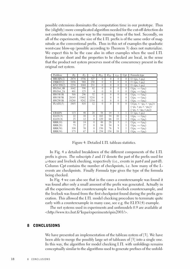
Problem BI EI cI BII EII cII Cpt Formula type

BRUIJN(2) 2874 1336 327 0 0 0 0 2¬(p1 ∧ p2)DIJKST(2) 1856 968 230 0 0 0 0 2¬(p1 ∧ p2)KNUTH(2) 2234 1044 251 0 0 0 0 2¬(p1 ∧ p2)BYZA4_0B 1642 590 82 0 0 0 0 2(p1 → 3p2)BYZA4_2A 401 125 4 0 0 0 0 2(p1 → 3p2)RW1W1R 568 296 32 0 0 0 0 2(p1 → 3p2)RW1W3R 28143 15402 5210 0 0 0 0 2(p1 → 3p2)RW2W1R 18280 9242 1334 0 0 0 0 2(p1 → 3p2)PLATE(5) 1803 810 12 0 0 0 0 2((p1 ∧ ¬p2 ∧ ¬p3)∨

(¬p1 ∧ p2 ∧ ¬p3)∨(¬p1 ∧ ¬p2 ∧ p3))

EBAHN 113 48 20 38 14 1 1 2¬(p1 ∧ p2)ELEV(3) 22 10 0 102 54 10 1 2(p1 → 3p2)ELEV(4) 25 12 0 129 68 13 1 2(p1 → 3p2)RRR(10) 40 14 0 48 28 5 1 2(p1 → 3p2)RRR(20) 73 27 0 94 54 8 1 2(p1 → 3p2)RRR(30) 104 38 0 136 76 9 1 2(p1 → 3p2)RRR(50) 173 67 0 234 134 18 1 2(p1 → 3p2)

Figure 4: Detailed LTL tableau statistics.

In Fig. 4 a detailed breakdown of the different components of the LTLprefix is given. The subscripts I and II denote the part of the prefix used forω-trace and livelock checking, respectively (i.e., events in part-I and part-II).Column Cpt contains the number of checkpoints, i.e. how many of the L-events are checkpoints. Finally Formula type gives the type of the formulabeing checked.

In Fig. 4 we can also see that in the cases a counterexample was found itwas found after only a small amount of the prefix was generated. Actually inall the experiments the counterexample was a livelock counterexample, andthe livelock was found from the first checkpoint found during the prefix gen-eration. This allowed the LTL model checking procedure to terminate quiteearly with a counterexample in many case, see e.g. the ELEV(4) example.

The net systems used in experiments and unfsmodels 0.9 are available at<http://www.tcs.hut.fi/˜kepa/experiments/spin2001/>.

8 CONCLUSIONS

We have presented an implementation of the tableau system of [3]. We havebeen able to merge the possibly large set of tableaux of [3] into a single one.In this way, the algorithm for model checking LTL with unfoldings remainsconceptually similar to the algorithms used to generate prefixes of the unfold-

18 8 CONCLUSIONS

ing containing all reachable states [6, 5]: We just need more sophisticatedadequate orders and cut-off events.

The division of the tableau into part-I and part-II events is the price topay for a partial-order approach to model checking. Other partial-order tech-niques, like the one introduced by Valmari [19], also require a special treat-ment of divergences or livelocks. 3 We have shown that the conditions forchecking if part-I or part-II events are terminals remain very simple.

In our tableau system the size of a tableau may grow quadratically in thenumber of reachable states of the system. We have not been able to constructan example showing that this bound can be reached, although it probably ex-ists. In all experiments conducted so far the number of events of the tableauis always smaller than the number of reachable states. In examples with ahigh degree of concurrency we obtain exponential compression factors.

The prototype implementation was created mainly for investigating thesizes of the generated tableau. Implementing this procedure in a high per-formance prefix generator such as the one described in [5] is left for furtherwork.

Acknowledgements

We would like to thank Claus Schröter for collecting the set of LTL modelchecking benchmarks used in this work. This work has been partially finan-cially supported by the Teilprojekt A3 SAM of the Sonderforschungsbereich342 “Werkzeuge und Methoden für die Nutzung paralleler Rechnerarchitek-turen”, the Academy of Finland (Projects 47754 and 43963), and the EmilAaltonen Foundation.

References

[1] J. C. Corbett. Evaluating deadlock detection methods for concurrentsoftware. Technical report, Department of Information and ComputerScience, University of Hawaii at Manoa, 1995.

[2] C. Courcoubetis, M. Y. Vardi, P. Wolper, and M. Yannakakis. Memory-efficient algorithms for the verification of temporal properties. FormalMethods in System Design, 1:275–288, 1992.

[3] J. Esparza and K. Heljanko. A new unfolding approach to LTL modelchecking. In Proceedings of 27th International Colloquium on Au-tomata, Languages and Programming (ICALP’2000), pages 475–486,July 2000. LNCS 1853.

[4] J. Esparza and K. Heljanko. A new unfolding approachto LTL model checking. Research Report A60, HelsinkiUniversity of Technology, Laboratory for Theoretical Com-puter Science, Espoo, Finland, April 2000. Available at<http://www.tcs.hut.fi/Publications/reports/A60abstract.html>.

3The idea of dynamically checking which L-transitions are checkpoints could also beused with the approach of [19] to implement state based LTL-X model checking.

REFERENCES 19

[5] J. Esparza and S. Römer. An unfolding algorithm for synchronous prod-ucts of transition systems. In Proceedings of the 10th InternationalConference on Concurrency Theory (Concur’99), pages 2–20, 1999.LNCS 1664.

[6] J. Esparza, S. Römer, and W. Vogler. An improvement of McMillan’sunfolding algorithm. In Proceedings of 2nd International Workshopon Tools and Algorithms for the Construction and Analysis of Systems(TACAS’96), pages 87–106, 1996. LNCS 1055.

[7] J. Esparza and C. Schröter. Reachability analysis using net unfold-ings. In Proceeding of the Workshop Concurrency, Specification &Programming 2000, volume II of Informatik-Bericht 140, pages 255–270. Humboldt-Universität zu Berlin, 2000.

[8] R. Gerth, D. Peled, M. Y. Vardi, and P. Wolper. Simple on-the-flyautomatic verification of linear temporal logic. In Proceedings of 15thWorkshop Protocol Specification, Testing, and Verification, pages 3–18,1995.

[9] M. Heiner and P. Deussen. Petri net based qualitative analysis - Acase study. Technical Report Technical Report I-08/1995, BrandenburgTechnische Universität Cottbus, Cottbus, Germany, December 1995.

[10] K. Heljanko. Deadlock and reachability checking with finitecomplete prefixes. Research Report A56, Helsinki University ofTechnology, Laboratory for Theoretical Computer Science, Es-poo, Finland, December 1999. Licentiate’s Thesis. Available at<http://www.tcs.hut.fi/Publications/reports/A56abstract.html>.

[11] K. Heljanko. Using logic programs with stable model semantics to solvedeadlock and reachability problems for 1-safe Petri nets. FundamentaInformaticae, 37(3):247–268, 1999.

[12] G. Holzmann. The model checker SPIN. IEEE Transactions on Soft-ware Engineering, 23(5):279–295, 1997.

[13] C. Lewerentz and T. Lindner. Formal Development of Reactive Sys-tems: Case Study Production Cell. Springer-Verlag, 1995. LNCS 891.

[14] K. L. McMillan. Symbolic Model Checking. Kluwer Academic Pub-lishers, 1993.

[15] S. Melzer and S. Römer. Deadlock checking using net unfoldings.In Proceedings of 9th International Conference on Computer-AidedVerification (CAV ’97), pages 352–363, 1997. LNCS 1254.

[16] S. Merkel. Verification of fault tolerant algorithms using PEP. Tech-nical Report TUM-19734, SFB-Bericht Nr. 342/23/97 A, TechnischeUniversität München, München, Germany, 1997.

[17] W. Reisig. Petri Nets, An Introduction. Springer-Verlag, 1985.

20 REFERENCES

[18] P. Simons. Extending and Implementing the Stable Model Semantics.PhD thesis, Helsinki University of Technology, Laboratory for Theoret-ical Computer Science, April 2000. Also available on the Internet at<http://www.tcs.hut.fi/Publications/reports/A58abstract.html>.

[19] A. Valmari. On-the-fly verification with stubborn sets. In Proceed-ing of 5th International Conference on Computer Aided Verification(CAV’93), pages 397–408, 1993. LNCS 697.

[20] M. Y. Vardi. An automata-theoretic approach to linear temporal logic.In Logics for Concurrency: Structure versus Automata, pages 238–265,1996. LNCS 1043.

[21] K. Varpaaniemi, K. Heljanko, and J. Lilius. PROD 3.2 - An advancedtool for efficient reachability analysis. In Proceedings of the 9th Inter-national Conference on Computer Aided Verification (CAV’97), pages472–475, 1997. LNCS 1254.

[22] F. Wallner. Model checking LTL using net unfoldings. In Proceed-ing of 10th International Conference on Computer Aided Verification(CAV’98), pages 207–218, 1998. LNCS 1427.

REFERENCES 21

9 APPENDIX A - PROOFS OF THEOREMS

We start with a lemma proving some additional properties of Σ¬ϕ.

Lemma 1 Let Σ¬ϕ be the net system defined through steps (1)-(6) in Sec-tion 3. On top of (a) and (b) in Theorem 1 Σ¬ϕ also satisfies the followingproperties:

(c) No reachable marking of Σ¬ϕ concurrently enables two different I -transitions.

(d) If a reachable marking of Σ¬ϕ concurrently enables two different tran-sitions, then none of them is an L-transition.

(e) After firing an L-transition all transitions in the sets L, V, and I staydisabled.

(f) If M is a marking reached without firing any L-transitions, and M ′ is amarking reached after firing some L-transitions, then M 6= M ′.

Proof:

(c) No reachable marking of Σ¬ϕ concurrently enables two different I -transitions.Just observe that all I -transitions have the place sf in their preset.

(d) If a reachable marking of Σ¬ϕ concurrently enables two different tran-sitions, then none of them is a L-transition.Let (q, s, O, H) be a reachable marking that concurrently enables anL-transition t and another transition u. Since the preset of t is also areachable marking (q, sf , O, H), we have q = q, s = sf , O ⊆ O, andH ⊆ H . Since all reachable markings of Σ are pairwise incompara-ble and (O, H), (O, H) are reachable markings of Σ, we have O = Oand H = H . Since u is enabled at (q, s, O, H), t and u have at leastone common place in their presets, and so they are not concurrentlyenabled.

(e) After firing an L-transition all transitions in the sets L, V, and I staydisabled forever.Is immediate from the fact that L-transitions do not put tokens on anyscheduling places, and a scheduling place is in the preset of all L, V ,and I -transitions.

(f) Let M be a marking reached without firing any L-transitions, and M ′

be a marking reached after firing some L-transitions. Then it holds thatM 6= M ′.After an L-transition has fired both scheduling places will stay empty,and before firing it exactly one of them contains a token.

ut

22 9 APPENDIX A - PROOFS OF THEOREMS

Proof of Theorem 2

We use the Lemma 1(d),(f) above in this proof.The totality follows directly from the fact that ≺ is a total order. It is easy

to see that ≺LTL is well founded. Also it it easy to see from the definitionthat C1 ⊂ C2 implies C1 ≺LTL C2 because this property holds for the ≺order. We now want to prove that ≺LTL is preserved by finite extensions. Weproceed by showing the claim for extension by a single event E = {e}, thefull claim will follow by induction. We have now two cases:

(1) C1 does not contain an L-event: Now Mark(C1) = Mark(C2) im-plies that C2 does not contain an L-event either (Lemma 1 (f)). ThusBL(C1) = C1, BL(C2) = C2, BL(C1 ⊕ E) = C1 ⊕ E, and BL(C2 ⊕f(E)) = C2 ⊕ f(E), and we obtain the result from the fact that ≺ ispreserved by finite extensions.

(2) C1 contains an L-event: Now Mark(C1) = Mark(C2) implies that C2

also contains an L-event. Thus BL(C1 ⊕ E) = BL(C1) because L-events are not concurrent with any other events (Lemma 1 (d)). Bythe same reasoning BL(C2 ⊕ f(E)) = BL(C2). We us this result in asimple case analysis of the ≺LTL definition:

(a) BL(C1) ≺ BL(C2): We get BL(C1⊕E) ≺ BL(C2⊕f(E)), andthus C1 ⊕ E ≺LTL C2 ⊕ f(E).

(b) BL(C1) = BL(C2) and C1 ≺ C2: Now it holds that BL(C1 ⊕E) = BL(C2 ⊕ f(E)) and C1 ⊕ E ≺ C2 ⊕ f(E). ThereforeC1 ⊕ E ≺LTL C2 ⊕ f(E).

Proof of Theorem 3

The proofs strategies here are similar to those in [3, 4]. However, technicaldetails differ enough that those proofs cannot be directly used here. Thus aself-contained proof is given.

We split Theorem 3 into five results contained in Theorem 4-Theorem 8.

Soundness and completeness for illegal ω-traces

Theorem 4 If T contains a successful terminal of type I, then Σ¬ϕ has anillegal ω-trace.

Proof:Let e be a successful terminal of T of type I with companion e′. In particular,

e′ < e, and so [e′] ⊂ [e]. Let M0σ

−−−→M1σ1−−−−→M2 be a firing sequence of

Σ¬ϕ such that σ and σσ1 are linearisations of [e′] and [e], respectively. SinceMark([e′]) = Mark([e]), we have M1 = M2. Since [e]\ [e′] contains some I -

event, M0σ

−−−→M1

σω1−−−−→ is an infinite firing sequence of Σ¬ϕ containing

infinitely many occurrences of transitions of I . ut

The proof of completeness is a bit more involved. We need a preliminarydefinition and a lemma.

9 APPENDIX A - PROOFS OF THEOREMS 23

Definition 5 A configuration C of the unfolding of Σ¬ϕ is bad if it containsat least K+1 I -events, where K is the number of reachable markings of Σ¬ϕ.

Lemma 2 (1) Σ¬ϕ has an illegal ω-trace if and only if its unfolding con-tains a bad configuration.

(2) A bad configuration contains at least one successful terminal of type I.(More precisely, if a branching process of Σ¬ϕ contains a bad configu-ration, then some event of this configuration is a terminal.)

Proof:(1) (⇒): Let M0

σ−−−→M be a prefix of an illegal ω-trace such that σ con-

tains K + 1 occurrences of I -transitions. There exists a configuration of theunfolding of Σ¬ϕ such that σ is a linearisation of C. This configuration isbad.

(1) (⇐): Let C be a bad configuration. C contains at least K + 1 I -events. By Lemma 1(c), these events are causally ordered, and so by thepigeonhole principle two of them e′ < e satisfy Mark([e′]) = Mark([e]). Let

M0σ1−−−−→M1

σ2−−−−→M2 be a linearisation of [e] such that σ1 is a linearisa-tion of [e′]. Then M1 = M2, and so σ1σ

ω2 is an illegal ω-trace.

(2) Event e in the proof of (1) (⇐) is a successful terminal of type I. ut

Theorem 5 If Σ¬ϕ has an illegal ω-trace then T has a successful terminal oftype I.

Proof:By Lemma 2(1), it suffices to show that if the unfolding of Σ¬ϕ contains abad configuration, then T has a successful terminal of type I.

We prove that, given a bad configuration C of the unfolding of Σ¬ϕ, eitherC contains a type I successful terminal of T (and so T itself contains a typeI successful terminal), or there exists another bad configuration C ′ such thatC ′ ≺LTL C. Since ≺LTL is well founded (see Definition 2), T contains atype I successful terminal.

By Lemma 2(2), C contains a successful terminal e of type I. If e belongsto T , then we are done. Otherwise, C must contain an unsuccessful terminald < e. Since e is of type I so is d. We have C = [d] ⊕ (C \ [d]). Let d′ bethe companion of d, and let f be an isomorphism between ↑ [d] and ↑ [d′].Define C ′ = [d′] ⊕ f(C \ [d]). We prove that C ′ is a bad configurationsatisfying C ′ ≺LTL C.

We consider two cases, corresponding to the two possibilities for a terminalof type I to be unsuccessful:

(a) d′ < d, and [d] \ [d′] contains no I -event.In this case we have [d′] ⊂ [d]. By the second condition in the definition ofan adequate order, we have [d′] ≺LTL [d]. By the third condition of the samedefinition, we have C ′ ≺LTL C.It remains to prove that C ′ is bad. We show that C and C ′ contain thesame number of I -events. Since [d] \ [d′] contains no I -event, we have#I [d

′] = #I [d]. Since isomorphisms preserve labelling, we have #I(C′ \

[d′]) = #I(C \ [d]). So #IC′ = #IC.


(b) [d′] ≺LTL [d] and #I [d′] ≥ #I [d].

Since [d′] ≺LTL [d], we have C ′ ≺LTL C by the third condition in the defini-tion of an adequate order. It remains to prove that C ′ is bad. We show that C ′

contains at least as many I -events as C. We have #I [d′] ≥ #I [d] by assump-

tion. Since isomorphisms preserve labelling, we also have #I(C′ \ [d′]) =

#I(C \ [d]). So #IC′ ≥ #IC. ut

Soundness for illegal livelocksWe start with some simple observations following directly from the defini-tions.

Lemma 3 Let C be a configuration.

(1) BL(C) contains at most one L-event. If BL(C) contains one L-event,then this event is the unique maximal event of BL(C).

(2) All events of AL(C) are invisible.

(3) If some linearisation of C is an illegal livelock M0σ

−−−→Mτ

−−−→, thenσ is a linearisation of BL(C).

Proof:(1) By the definition of BL, all L-events of BL(C) are maximal events ofBL(C). Since L-transitions are never concurrently enabled with any othertransition (Lemma 1(d)), BL(C), the set of maximal events of BL(C) eithercontains no L-events, or it consists of exactly one L-event.(2) Follows easily from the definition of AL and Lemma 1(e).(3) Since the last transition of σ is a L-transition, C contains one L-event. By(1), this is the unique maximal event of BL(C). ut

The following lemma is also a preliminary.

Lemma 4 Let C1, C2 be configurations of the unfolding of a 1-safe net sys-tem Σ such that C1∪C2 is a configuration, and Mark(C1) = M = Mark(C2).Then Mark(C1 ∩ C2) = M .

Proof:Let c1, c2, c12 be the cuts corresponding to C1, C2, and C1 ∩C2, respectively.

(1) If p ∈ M , then p ∈ Mark(C1 ∩ C2).Since p ∈ M , there exist b1 ∈ c1, b2 ∈ c2 such that l(b1) = p = l(b2). SinceΣ is 1-safe, b1 and b2 cannot be concurrent. Since C1∪C2 is a configuration,they must be causally related. Assume without loss of generality that b1 ≤ b2.Then b1 ∈ c12, and so p ∈ Mark(C1 ∩ C2).

(2) If p ∈ Mark(C1 ∩ C2), then p ∈ M .Since p ∈ Mark(C1 ∩ C2), there exists b ∈ c12 such that l(b) = p. Thenb ∈ c1 ∪ c2, and so p ∈ Mark(C1) or p ∈ Mark(C2). Since Mark(C1) =M = Mark(C2), we have p ∈ M . ut

We can now prove the soundness of the tableau for illegal livelocks.

Theorem 6 If T contains a successful terminal of type II, then Σ¬ϕ containsan illegal livelock.


Proof:Let e be the successful terminal and let e′ be its companion. Since e isof type II(b) we have BL([e′]) = BL([e]), and so e′ is a part-II event. Let

M0σ1−−−−→M1

σ2−−−−→M2σ3−−−−→M3 be a linearisation of [e] such that σ1 is

a linearisation of BL([e]), and σ1σ2 is a linearisation of [e] ∩ [e′]. (Noticethat σ2 is a non-empty sequence.) By Lemma 3(1), the last transition of σ1

belongs to L. Since ¬(e′#e), [e] ∪ [e′] is a configuration and so, by Lemma4, Mark([e]) = Mark([e] ∩ [e′]), i.e., M2 = M3. Since σ1 is a linearisa-tion of BL([e]) and σ1σ2σ3 is a linearisation of [e], σ2 contains only invisible

transitions (Lemma 3(2)). So M0σ1−−−−→M1

σ2σω3−−−−−→ is an illegal livelock of

Σ¬ϕ. ut

Completeness for the illegal livelocksThe completeness proof uses the following notion:

Definition 6 A configuration C is a L-configuration if BL(C) 6= ∅ andAL(C) contains at least K + 1 events, where K is the number of reachablemarkings of Σ¬ϕ.

Loosely speaking, the following lemma shows that L-configurations arefinite witnesses of the existence of illegal livelocks.

Lemma 5 Σ¬ϕ has an illegal livelock M0σ

−−−→Mτ

−−−→ if and only if its un-folding contains a L-configuration C such that σ is a linearisation of BL(C).

Proof:(⇒): Let M0

σ−−−→M

τ−−−→ be a livelock of Σ¬ϕ, i.e.,

• the last transition of σ belongs to L, and

• τ is an execution containing only invisible transitions.

Let C be an (infinite) configuration of the unfolding of Σ¬ϕ such that στis one of its linearisations. By Lemma 3(3), σ is a linearisation of BL(C).Since C is infinite, AL(C) contains infinitely many events. Let BL(C)⊕ Ebe an extension of BL(C) such that E contains K + 1 events; BL(C) ⊕ Eis a L-configuration.

(⇐): Let C be a L-configuration, and let M0σ1−−−−→M1 be a linearisation

of BL(C). By Lemma 3(1), the last transition of σ1 is labelled by a transition

of L. We construct an execution M1σ2σω

3−−−−−→ of invisible transitions, which

implies that M0σ

−−−→ M1σ2σω

3−−−−−→ is an illegal livelock. Since AL(C)contains at least K + 1 events, there exist two events e′, e ∈ AL(C) such thatMark(e′) = Mark(e). Let M0

σ1−−−−→M1σ2−−−−→M2

σ3−−−−→M3 be a lineari-sation of [e] such that M0

σ1−−−−→M1σ2−−−−→M2 is a linearisation of [e] ∩ [e′].

By Lemma 4 we have M2 = M3, and so M0σ1−−−−→M1

σ2σω3−−−−−→ is an ex-

ecution; since, by Lemma 3(2), σ3 only contains invisible transitions, thisexecution is an illegal livelock. ut

Loosely speaking, our next lemma shows that L-configurations lead to ter-minals in the tableau system.


Lemma 6 Every L-configuration contains a successful terminal of type II.

Proof:Since AL(C) contains at least K + 1 events, there exist two events e′, e ∈AL(C) such that Mark(e′) = Mark(e). Since e′, e ∈ AL(C), BL([e′]) =BL(C) = BL([e]). Without loss of generality we assume e′ ≺LTL e (recallthat ≺LTL is a total order). Since e′, e ∈ C we have ¬(e′#e), and so e is asuccessful terminal of type II. ut

Theorem 7 If Σ¬ϕ contains an illegal livelock then T contains a successfulterminal of type II.

Proof:By Lemma 5 the unfolding of Σ¬ϕ contains some L-configuration C. ByLemma 6, C contains a successful terminal e of type II.

We prove the following: either T contains a type II successful terminalof C, or the unfolding of Σ¬ϕ contains another L-configuration C ′ ≺LTL C.Since ≺LTL is well founded, T must contain a type II successful terminal.

If T does not contain any type II successful terminals, then in particularit does not contain e, and so T must contain an terminal d < e which is notof type II(b).

We construct an L-configuration C ′ ≺LTL C. We consider three possiblecases, corresponding to the three possibilities for a terminal to be unsuccess-ful.

(1) d is a terminal of type I(a) or I(b).Let d′ be the companion of d. Since Mark([d′]) = Mark([d]), there is anisomorphism f from ↑[d] to ↑[d′]. Define C ′ = [d′] ∪ f(C \ [d]). Since d isa part-I event (in particular d is not an L-event), we have BL(C) = [d] ⊕ Efor some nonempty set of events E. It holds that BL(C ′) = [d′] ⊕ f(E)and AL(C ′) = f(AL(C)). Since E is nonempty, we have BL(C ′) 6= ∅.Since AL(C ′) = f(AL(C)), we have |AL(C ′)| = |AL(C)|, and so AL(C ′)contains at least K + 1 events. Since [d′] ≺LTL [d] and ≺LTL is preserved byfinite extensions, we have BL(C ′) ≺LTL BL(C), and so C ′ ≺LTL C.

(2) d is a terminal of type II(a).Let d′ be the companion of d. Since d is a terminal of type II(a), it is a part-IIevent. By Lemma 1(f), d′ is also a part-II event. By Lemma 3(3), Σ¬ϕ has an

illegal livelock M0σ

−−−→Mσ1−−−−→ such that σ is a linearisation of BL(C).

We split σ1 into two sequences, σ1 = σ2σ3, such that σσ2 is a linearisationof [d], and so

M0σ

−−−→Mσ2−−−−→Mark([d])

σ3−−−−→

Now find a linearisation σ′σ′2 of [d′] such that M0σ′

−−−→M ′σ′2−−−−→Mark([d′]).

So we have

M0σ′

−−−→M ′σ′2−−−−→Mark([d′]) = Mark([d])

σ3−−−−→

which is an illegal livelock of Σ¬ϕ. By Lemma 5, there is a L-configurationC ′ such that σ′ is a linearisation of BL(C ′). It remains to prove C ′ ≺LTL C.Since σ′ is a prefix of σ′σ′2, we have BL(C ′) ⊆ [d′]. We now have

BL(C ′) = BL([d′]) (BL(C ′) ⊆ [d′])≺LTL BL([d]) (d is of type II(a))

= BL(C) (BL(C) ⊆ [d])


It follows C ′ ≺LTL C (definition of ≺LTL).(3) d is a terminal of type II(c).

Let d′ be the companion of d. Since Mark([d′]) = Mark([d]), there is anisomorphism f from ↑[d] to ↑[d′]. Define C ′ = [d′] ∪ f(C \ [d]).

We first prove BL(C ′) = BL(C). Since d is a terminal of type II(c), it is apart-II event. By Lemma 1(f), d′ is also a part-II event. So we have BL(C) =BL([d]) and BL(C ′) = BL([d′]). Since d is of type II(c), BL([d′]) =BL([d]), and we are done.

We now show that C ′ is a L-configuration such that C ′ ≺LTL C. SinceC is a L-configuration, BL(C) 6= ∅, and so, since BL(C ′) = BL(C),BL(C ′) 6= ∅. Since [d] is a terminal of type II(c), we have |[d′]| ≥ |[d]|,and so, since BL([d]) = BL([d′]), |AL(C ′)| ≥ |AL(C)|. Since C is a L-configuration, |AL(C)| ≥ K + 1. Finally, C ′ ≺LTL C is proved exactly as incase (2). ut

Finiteness of the tableau

We will now proceed to prove the following

Theorem 8 T contains at most K2 non-terminal events, where K is thenumber of reachable markings of Σ¬ϕ.

Using Lemma 1(f) we get that the reachable markings of Σ¬ϕ can be di-vided into to disjoint sets, marking reachable by firing no L-transitions andmarkings reachable after firing some L-transition. Let KI and KII respec-tively denote the number of these markings, and so K = KI + KII .

We first consider the size of part-I.

Lemma 7 T contains at most KI2 non-terminal part-I events.

Proof:We proceed in three steps.

(1) Let C be an configuration of T containing only part-I events. If C con-tains more than KI events labelled by transitions of I , then C containsa terminal.Since all events labelled by transitions of I are causally related (see theLemma 1(c)), C contains a chain e1 < . . . < eKI+1 of such events. Bythe pigeonhole principle, there are events ei < ej , 1 ≤ i, j ≤ KI + 1,such that Mark([ei]) = Mark([ej]). Now ej is a type I terminal.

(2) Let M be a reachable marking of Σ¬ϕ without firing any L-transitions.T contains at most KI non-terminal part-I events e such that Mark(e) =M .Assume the contrary, and let e1 . . . eKI+1 be pairwise different non-terminal part-I events such that Mark(ei) = M for all 1 ≤ i ≤ KI + 1.By (1), we have #I [ei] ≤ KI for all 1 ≤ i ≤ KI + 1. So there aretwo indices i 6= j such that #I [ei] = #I [ej]. Since ≺LTL is a totalorder, we have either [ei] ≺ [ej] or [ej] ≺ [ei]. So by the definition ofterminals of type I either ei or ej is a type I terminal.


(3) T contains at most KI2 non-terminal part-I events.

By (2), T contains at most KI non-terminal part-I events for each mark-ing reachable without firing L-transitions, and so there are at most KI

2

non-terminal part-I events.ut

We next consider the size of part-II.

Lemma 8 T contains at most KII2 non-terminal part-II events.

Proof:We use the same pattern as above and proceed in three steps.

(1) Let C be an configuration T containing some part-II events. If |AL(C)| >KII , then C contains a terminal.If |AL(C)| > KII , then C contains two part-II events e′, e such that¬(e′#e) and Mark([e′]) = Mark([e]). By the definition of terminalsof type II(b), e′ or e is a terminal.

(2) Let M be a reachable marking of Σ¬ϕ after firing some L-transition. Tcontains at most KII non-terminal part-II events e such that Mark(e) =M .Assuming the contrary, let E be a set containing more than KII non-terminal part-II events such that Mark(e) = M for all e ∈ E. By (1),we have |AL([e])| ≤ KII for all e ∈ E. By the pigeonhole principle,there are two different events e1, e2 such that |AL([e1])| = |AL([e2])|.We show that e1 or e2 is a terminal of type II. There are two possiblecases:

(a) BL([e1]) 6= BL([e2]).If BL([e1]) ≺LTL BL([e2]) then e2 is a terminal (of type II(a)),otherwise e1 is a terminal (of type II(a)).

(b,c) BL([e1]) = BL([e2]).Now BL([e1]) = BL([e2]) and |AL([e1])| = |AL([e2])| implies|[e1]| = |[e2]|. Thus the larger one with respect to ≺LTL is aterminal (of type II(b) or II(c)).

Therefore either e1 or e2 is a terminal, a contradiction.

(3) T contains at most KII2 non-terminal part-II events.

By (2), T contains at most KII non-terminal part-II events for eachmarking reachable after firing some L-transition, and so there are atmost KII

2 non-terminal part-II events.ut

Now by Lemmas 7 and 8 we get that T contains at most KI2+KII

2 ≤ K2

non-terminal events. ut


HELSINKI UNIVERSITY OF TECHNOLOGY LABORATORY FOR THEORETICAL COMPUTER SCIENCE

RESEARCH REPORTS

HUT-TCS-A55 Tommi Syrjanen

A Rule-Based Formal Model For Software Configuration. December 1999.

HUT-TCS-A56 Keijo Heljanko

Deadlock and Reachability Checking with Finite Complete Prefixes. December 1999.

HUT-TCS-A57 Tommi Junttila

Detecting and Exploiting Data Type Symmetries of Algebraic System Nets during

Reachability Analysis. December 1999.

HUT-TCS-A58 Patrik Simons

Extending and Implementing the Stable Model Semantics. April 2000.

HUT-TCS-A59 Tommi Junttila

Computational Complexity of the Place/Transition-Net Symmetry Reduction Method.

April 2000.

HUT-TCS-A60 Javier Esparza, Keijo Heljanko

A New Unfolding Approach to LTL Model Checking. April 2000.

HUT-TCS-A61 Tuomas Aura, Carl Ellison

Privacy and accountability in certificate systems. April 2000.

HUT-TCS-A62 Kari J. Nurmela, Patric R. J. Ostergard

Covering a Square with up to 30 Equal Circles. June 2000.

HUT-TCS-A63 Nisse Husberg, Tomi Janhunen, Ilkka Niemela (Eds.)

Leksa Notes in Computer Science. October 2000.

HUT-TCS-A64 Tuomas Aura

Authorization and availability - aspects of open network security. November 2000.

HUT-TCS-A65 Harri Haanpaa

Computational Methods for Ramsey Numbers. November 2000.

HUT-TCS-A66 Heikki Tauriainen

Automated Testing of Buchi Automata Translators for Linear Temporal Logic.

December 2000.

HUT-TCS-A67 Timo Latvala

Model Checking Linear Temporal Logic Properties of Petri Nets with Fairness Constraints.

January 2001.

HUT-TCS-A68 Javier Esparza, Keijo Heljanko

Implementing LTL Model Checking with Net Unfoldings. March 2001.

ISBN 951-22-5390-9

ISSN 1457-7615

Documents

IMPLEMENTING LTL MODEL CHECKING WITH NET UNFOLDINGS