Implementation of Square Root FunctionUsing Quantum Circuits

Computer Science Junior Independent Work

Pranav GokhalePrinceton University Class of 2015

Advised by Dr. Iasonas Petras

January 12, 2014

Abstract

The design of quantum circuits that implement elementary func-

tions has foundational value for the field of quantum computing and

is also important for the development of other quantum algorithms.

Here, we present the first design for a quantum circuit that computes

the square root of any number v > 1. We include error analysis

and asymptotic estimates for complexity and resource requirements.

Specifically, if a total error of at most E is desired, then the pro-

cedure requires order O(log2 log26v1.5

E ) iterations and a maximum of

O(log2v1.5

E ) qubits at any particular stage. A preliminary design for

a circuit extension computing vz for other fractional powers (besides

z = 1/2) is also presented, as well as for the special case where z is a

power of 2.

1

1 Introduction

Quantum computing is an emerging field that presents a fundamentally new

model of computation. Although no scalable quantum computers have been

built yet, it is important to study the theory of quantum computing to un-

derstand what the capabilities of a quantum computer will be. In certain

instances, quantum algorithms can provide exponential speedups over classi-

cal algorithms. For example, a quantum computer can run Shor’s algorithm

[4] to factor an integer in polynomial time with the input size, whereas the

best known classical algorithms require at least subexponential time. More

recently, quantum algorithms have been proposed that can efficiently solve

problems that suffer from the “curse-of-dimensionality” under certain as-

sumptions. For instance, numerically solving a Poisson equation problem

has complexity that is exponential with dimension for a classical computer

but there is a quantum algorithm with cost linear in the problem’s dimension

[2].

As the field of quantum computing grows, it is becoming increasingly

important to design quantum circuits that implement elementary functions.

Apart from the intrinsic value in being able to perform the most fundamen-

tal operations, the implementations of more complicated quantum algorithms

are often predicated on the existence of circuit modules for elementary func-

tions. For example, a quantum circuit design for elementary arithmetic oper-

ations [6] is vital for the implementation of the numerous quantum algorithms

2

involving addition, multiplication, and exponentiation. Similarly, the quan-

tum algorithm for various partial differential equation problems [2] requires

circuits for reciprocals, sines, and cosines. Last but not least, there has also

been focus on developing standardized quantum circuit modules from the

IARPA (Intelligence Advanced Research Projects Agency) Quantum Com-

puter Science Program [3], which seeks to catalog the precise circuit resource

costs and error analyses of quantum algorithms.

2 Background

In this paper, we present the design for a quantum circuit that takes input

v > 1 and outputs an approximation of its square root,√v. Square roots can

be efficiently computed on a classical computer with the Babylonian method

(a special case of Newton’s method). The recurrence formula is

xi+1 =xi + v/xi

2

so that limi→∞ xi =√v. However, this does not translate into a practical

quantum circuit, because the v/xi term involves a new division at each stage

of the iteration. Because quantum circuits for division are generally avoided,

the Babylonian method cannot be directly used for a quantum circuit for

division. Similarly, approximating the square root function with a Taylor

series does not work, because the error grows rapidly away from the expansion

3

point and the formula also requires unwieldy divisions. It is also not sufficient

to merely input v into a classical computer, because if |v〉 is a superposition

of more than one state, the classical computer would collapse it into just

one of the states of the superposition. Thus, a proper quantum circuit for

approximating the square root should be able to accept a superposition state

and output the correct superposition state.

Another challenge for quantum circuits is that they must be built with

reversible logical components so that the quantum circuit involves a bijective

mapping from input to output. This means that the logical gates can only be

represented by unitary matrices [1]. While there is a reversible square root

circuit design for 8-bit input [7], the design is specific to the input size and

cannot be generalized to input of any size. Moreover, rigorous error analysis

has not been carried out for this reversible circuit. Another reversible square

root circuit proposal [5] claims to be extendible to arbitrary input size, but

specifics of the requisite internal modules have not been published and no

error analysis has been completed.

The approach used here involves first approximating 1/v via an inver-

sion circuit and then applying an inverse square root circuit to approximate

√v. The Newton method iterations for approximating these terms require

only division by two, multiplication, and addition, which are all manageable.

4

3 Inversion Circuit

We first compute xs1 , which approximates 1/v. The relevant quantum circuit

design and error analysis has been completed as a step in a quantum algo-

rithm for solving the Poisson equation [2]. The Newton iteration is shown in

Figure 1. The total error after s1 iterations, when using b1 bits of accuracy

(bits after the binary point), is bounded as

|xs1 − 1/v| ≤ 2−2s1 + s12

−b1 [2,Thm B.1]

|xi〉xi+1 = −vx2i + 2xi

|xi+1〉|v〉 |v〉

Figure 1: Circuit implementing each iteration step of the Newton methodfor the inversion stage

4 Inverse Square Root Circuit

4.1 Initial Approximation

Next, we compute ys2 , which approximates 1/√xs1 . As an initial approxima-

tion for 1/√xs1 , we take y0 = y0 = 2b(p−1)/2c, where 2−p ≤ xs1 < 2−p+1, p ∈ Z.

The initial approximation circuit finds the most significant bit of xs1 that is

1 (this bit is in the 2−p position of xs1) and sets a 1 in the 2b(p−1)/2c bit

position of y0. An ancilla qubit acts as a flag for whether a 1 has been set in

5

y0. A small circuit for two-qubit input is demonstrated in Figure 2. When

the ancilla qubit is |1〉, the circuit has no effect, |0〉|1〉|r1r0〉 → |0〉|1〉|r1r0〉.

When the ancilla qubit is |0〉, the action of the circuit is |0〉|0〉|r1r0〉 →

|r1 OR r0〉|r1 OR r0〉|r1r0〉. Thus, |s0〉 is set to |1〉 if and only if the ancilla

is 0 and r1 or r0 is 1.

|s0 = 0〉 • •

|ancilla〉

|r1〉 •

|r0〉 •Figure 2: Small example of a circuit computing the initial approximationy0 = 2b(p−1)/2c of Newton iteration for approximating 1/

√xs1 , where 2−p ≤

xs1 < 2−p+1, p ∈ Z. In this example, xs1 is the two qubit input 0.r1r0 andy0 = s0.0

The circuit in Figure 2 is the building block for the general circuit in

Figure 3 which is extendible to arbitrary input size. Because this circuit is

composed of reversible logic gates, it can act on superpositions of inputs and

produce superposition output states as well.

6

|sn′−1 = 0〉 . . . • •

|y0〉......

|s0 = 0〉 • • . . .

|0〉 . . . X |0〉

|rn−1〉 • . . .

|rn−2〉 • . . .

|xs1〉...

...

|r1〉 . . . •

|r0〉 . . . •Figure 3: The quantum circuit computing the initial approximation y0 =2b(p−1)/2c of Newton iteration for approximating 1/

√xs1 , where 2−p ≤ xs1 <

2−p+1. Here, xs1 = 0.rn−1rn−2...r1r0 and y0 = sn′−1sn′−2...s1s0.0. The lengthof y0 is n′ = b(n− 1)/2c+ 1 = b(n+ 1)/2c, where n is the length of xs1 .

4.2 Newton’s Method Iteration

Next, we apply Newton’s method with the function g(y) = 1/y2− xs1 (which

has root y = 1/√xs1 as desired). The recurrence is

ϕ(yi) = yi+1 = yi −g(yi)

g′(yi)= yi −

1/y2i − xs1−2/y3i

=3yi − xs1y3i

2.

Thus, we apply s2 iterations of the circuit in Figure 4 to attain ys2 , an approx-

imation for 1/√xs1 . This recurrence requires quantum circuits for addition

7

and multiplication, which have been previously studied [6]. The recurrence

also requires division by 2 which could, for example, be implemented using a

form of right shifting in a quantum register extended by one qubit set to |0〉.

|yi〉yi+1 = (3yi − xs1y3i )/2

|yi+1〉

|xs1〉 |xs1〉

Figure 4: Circuit implementing each iteration step of the Newton methodfor the inverse square root stage.

4.3 Error Analysis

Lemma 1. The only possible equilibrium values for the Newton’s method

recurrence are −1/√xs1 , 0, 1/

√xs1.

Proof. The recurrence reaches an equilibrium when yi+1 = ϕ(yi) = yi. Thus,

ϕ(yi) =3yi − xs1y3i

2= yi.

This equation has solutions yi = −1/√xs1 , 0, 1/

√xs1 .

Lemma 2. For y0 ∈ (0, 1/√xs1 ], the recurrence will maintain the invariant,

yi ∈ (0, 1/√xs1 ].

Proof. We have the Newton iteration function ϕ(yi) = yi+1 = (3yi−xs1y3i )/2.

Since ϕ is continuous, it must have a maximum over the domain [0, 1/√xs1 ].

The derivative, ϕ′(yi) = (3−3xs1y2i )/2, is 0 over this domain at yi = 1/

√xs1 .

8

Evaluating ϕ(yi) at yi = 0 and yi = 1/√x, we find by the Extreme Value

Theorem that ϕ has a maximum value on this domain of 1/√xs1 (at endpoint

yi = 1/√xs1).

Since ϕ(yi) is always positive for y0 ∈ (0, 1/√xs1 ], this means that

0 < yi+1 ≤ 1/√xs1 and thus we inductively know that the property holds for

all subsequent yi. Moreover, we are assured by Lemma 1 that for y0 in this

range, the recurrence can only converge to 1/√xs1 (which is the only point

in this range where yi+1 = yi).

Lemma 3. The Newton iteration error, ei = |yi − 1/√xs1|, satisfies

ei+1 =3e2i√xs1 − xs1e3i

2

Proof. By Lemma 2, ei = |yi − 1/√xs1| = 1/

√xs1 − yi. The error of the

next term is ei+1 = |yi+1 − 1/√xs1 | = 1/

√xs1 − (3yi − xs1y3i )/2. Indeed, we

have,

3e2i√xs1 − xs1e3i

2=

3(1/√xs1 − yi)2

√xs1 − xs1(1/

√xs1 − yi)3

2=

3(1/xs1 + y2i − 2yi/√xs1)

√xs1

2(contd.)

−xs1(1/(xs1

√xs1)− y3i + 3y2/

√xs1 − 3y/xs1)

2=

1√xs1− 3yi − xs1y3i

2= ei+1.

9

Lemma 4. The Newton iteration error satisfies the bound

ei <

(3

2e0√xs1

)2i

Proof. Since ei > 0 and xs1 > 0, we have

ei+1 =3e2i√xs1 − xs1e3i

2<

3e2i√xs1

2.

Unfolding this recurrence, we have

ei <

(3

2

)2i−1

(e0)2i(√xs1)

2i−1 <

(3

2e0√xs1

)2i

.

This error will converge to 0 if (32e0√xs1) < 1, or equivalently if e0 <

2/(3√xs1).

Lemma 5. For the stated initial approximation, the error of the Newton

method after i iterations satisfies

ei < (.75)2i

Proof. We use the initial approximation, y0 = y0 = 2b(p−1)/2c, where 2−p ≤

xs1 < 2−p+1, p ∈ Z. Thus, 2p/2−1 ≤ y0 ≤ 2(p−1)/2 and 2−p/2 ≤√xs1 <

10

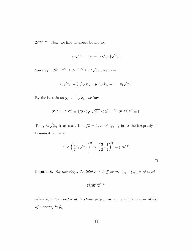
2(−p+1)/2. Now, we find an upper bound for

e0√xs1 = |y0 − 1/

√xs1|√xs1 .

Since y0 = 2b(p−1)/2c ≤ 2(p−1)/2 ≤ 1/√xs1 , we have

e0√xs1 = (1/

√xs1 − y0)

√xs1 = 1− y0

√xs1 .

By the bounds on y0 and√xs1 , we have

2p/2−1 · 2−p/2 = 1/2 ≤ y0√xs1 ≤ 2(p−1)/2 · 2(−p+1)/2 = 1.

Thus, e0√xs1 is at most 1 − 1/2 = 1/2. Plugging in to the inequality in

Lemma 4, we have

ei <

(3

2e0√xs1

)2i

≤(

3

2· 1

2

)2i

= (.75)2i

.

Lemma 6. For this stage, the total round off error, |ys2 − ys2|, is at most

(9/8)s223−b2

where s2 is the number of iterations performed and b2 is the number of bits

of accuracy in ys2.

11

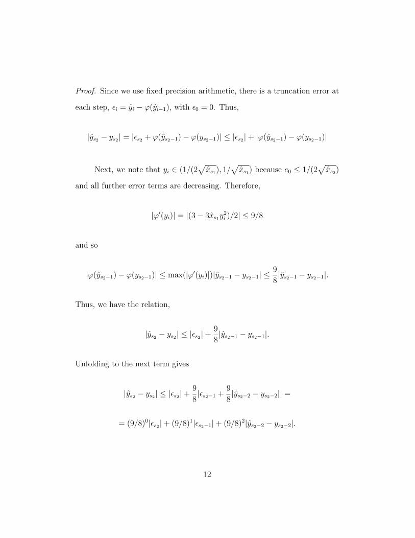
Proof. Since we use fixed precision arithmetic, there is a truncation error at

each step, εi = yi − ϕ(yi−1), with ε0 = 0. Thus,

|ys2 − ys2| = |εs2 + ϕ(ys2−1)− ϕ(ys2−1)| ≤ |εs2|+ |ϕ(ys2−1)− ϕ(ys2−1)|

Next, we note that yi ∈ (1/(2√xs1), 1/

√xs1) because e0 ≤ 1/(2

√xs2)

and all further error terms are decreasing. Therefore,

|ϕ′(yi)| = |(3− 3xs1y2i )/2| ≤ 9/8

and so

|ϕ(ys2−1)− ϕ(ys2−1)| ≤ max(|ϕ′(yi)|)|ys2−1 − ys2−1| ≤9

8|ys2−1 − ys2−1|.

Thus, we have the relation,

|ys2 − ys2| ≤ |εs2|+9

8|ys2−1 − ys2−1|.

Unfolding to the next term gives

|ys2 − ys2| ≤ |εs2|+9

8|εs2−1 +

9

8|ys2−2 − ys2−2|| =

= (9/8)0|εs2|+ (9/8)1|εs2−1|+ (9/8)2|ys2−2 − ys2−2|.

12

Fully unfolding the recurrence, we have

|ys2 − ys2| ≤s2∑i=1

(9/8)s2−i|εi|.

With b2 bits of accuracy, |εi| ≤ 2−b2 and we further have

|ys2 − ys2| ≤ 2−b2s2∑i=1

(9/8)s2−i = 2−b2s2−1∑i=0

(9/8)i =

= 2−b21− (9/8)s2

1− 9/8≤ (9/8)s223−b2

5 Total Error

We can bound the total error by

|ys2 −√v| ≤ |ys2 − 1/

√xs1|+ |1/

√xs1 −

√v|.

Now suppose we desire a total error of at most E. We can split the error

across these two terms so that each contributes an error of at most E/2.

By Lemma 5 and Lemma 6, we know that the first term is bounded by

the sum of the Newton iteration and round off errors for the inverse square

root stage,

|ys2 − 1/√xs1| ≤ (.75)2

s2 + (9/8)s223−b2 .

13

Next, we further split the desired error E/2 across these two terms, so that

each contributes an error of at most E/4. Thus, we first have

(.75)2s2 ≤ E

4

or

s2 = dlog2 log4/3

4

Ee

For the next term, we have

(9/8)s223−b2 = (9/8)dlog2 log4/34Ee23−b2 ≤ E

4

so that

b2 = 3 + dlog2

4

E+ log2

9

8dlog2 log4/3

4

Eee.

Now, we also desire an error of at most E/2 for the second absolute

value term, |1/√xs1 −

√v|. By Lemma 7 below, setting |xs1 − 1/v| ≤

E/(3v1.5) is sufficient so that |1/√xs1 −

√v| ≤ E/2.

Since |xs1 − 1/v| ≤ 2−2s1 + s12

−b1 [2, Thm B.1], we can split an error

of E/(3v1.5) between these two terms. Thus,

2−2s1 ≤ 1

2

E

3v1.5

and

s1 = dlog2 log2

6v1.5

Ee.

14

For the final term, we have

s12−b1 = dlog2 log2

6v1.5

Ee2−b1 ≤ 1

2

E

3v1.5

so that

b1 = dlog2

6v1.5

E+ log2dlog2 log2

6v1.5

Eee.

Lemma 7. If

|xs1 − 1/v| ≤ E

3v1.5

then

|1/√xs1 −

√v| < E

2.

Proof. We start with

|xs1 − 1/v| ≤ E

3v1.5.

Multiplying the left hand side by v/(√

xs1(1 +√vxs1)

)yields

|xs1 − 1/v| · v√xs1(1 +

√vxs1)

=

∣∣∣∣∣1−√vxs1√xs1

∣∣∣∣∣ =

∣∣∣∣∣ 1√xs1−√v

∣∣∣∣∣so we have

∣∣∣∣∣ 1√xs1−√v

∣∣∣∣∣ ≤ E

3v1.5· v√

xs1(1 +√vxs1)

=E

3√v· 1√

xs1(1 +√vxs1)

.

15

Since |xs1 − 1/v| ≤ E/(3v1.5), the denominator of the last term is equal to

at least √1/v − E/(3v1.5)

(1 +

√v(1/v − E/(3v1.5))

).

Moreover, since E <√v (otherwise y = 0 would be an immediate and trivial

approximation for√v that would satisfy the desired error), this is at least

√1/v −

√v/(3v1.5)

(1 +

√v(1/v −

√v/(3v1.5)

))=

=√

1/v − 1/(3v)(

1 +√v(1/v − 1/(3v))

)=

=

√2

3v

(1 +

√2

3

)=

(2

3+

√2

3

)· 1√

v

Returning to the inequality, we have

∣∣∣∣∣ 1√xs1−√v

∣∣∣∣∣ ≤ E

3√v· 1√

xs1(1 +√vxs1)

≤ E

3√v· 1

(2/3 +√

2/3)/√v≤ E

2.

And so we indeed have the final inequality,

∣∣∣∣∣ 1√xs1−√v

∣∣∣∣∣ < E

2.

16

6 Total Cost

Lemma 8. The total number of iterations required is of order O(log2 log26v1.5

E).

Proof. To achieve a total error, |ys2 −√v|, of at most E, we require s1 =

dlog2 log26v1.5

Ee = O(log2 log2

6v1.5

E) iterations of the inverse circuit and s2 =

dlog2 log4/34Ee = O(log2 log2

4E

) iterations of the inverse square root circuit.

s1 is asymptotically greater than s2 and the total number of iterations re-

quired to achieve an error of E is thus of order O(log2 log26v1.5

E).

Lemma 9. The maximum number of qubits required in the circuit at any

particular stage is of order O(log2v1.5

E).

Proof. Initially, storing the input v requires dlog2 ve qubits. The inversion

stage requires b1 = dlog26v1.5

E+ log2dlog2 log2

6v1.5

Eee = O(log2

v1.5

E) bits of

accuracy. The final inverse square root stage requires b2 = 3 + dlog24E

+

log298dlog2 log4/3

4Eee = O(log2

4E

) qubits at the beginning and end of each

iteration. Since the first term, O(log2v1.5

E) is asymptotically largest, we con-

clude that the maximum number of qubits required in the circuit at any

particular stage is of order O(log2v1.5

E).

Lemma 10. The total number elementary operations (single and singly-

controlled gates) required is of order O((log2v1.5

E)3 log2 log2

6v1.5

E), a low degree

polynomial in b1 and s1.

Proof. The initial approximation circuits for the inversion stage requires one

17

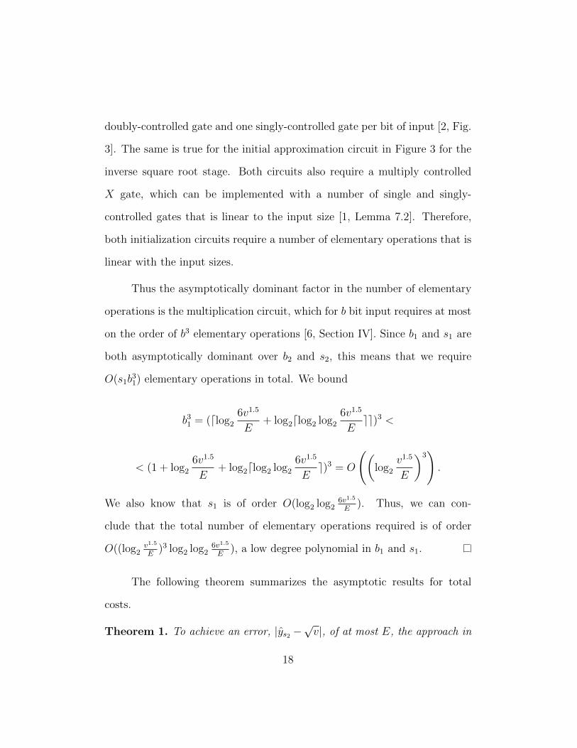
doubly-controlled gate and one singly-controlled gate per bit of input [2, Fig.

3]. The same is true for the initial approximation circuit in Figure 3 for the

inverse square root stage. Both circuits also require a multiply controlled

X gate, which can be implemented with a number of single and singly-

controlled gates that is linear to the input size [1, Lemma 7.2]. Therefore,

both initialization circuits require a number of elementary operations that is

linear with the input sizes.

Thus the asymptotically dominant factor in the number of elementary

operations is the multiplication circuit, which for b bit input requires at most

on the order of b3 elementary operations [6, Section IV]. Since b1 and s1 are

both asymptotically dominant over b2 and s2, this means that we require

O(s1b31) elementary operations in total. We bound

b31 = (dlog2

6v1.5

E+ log2dlog2 log2

6v1.5

Eee)3 <

< (1 + log2

6v1.5

E+ log2dlog2 log2

6v1.5

Ee)3 = O

((log2

v1.5

E

)3).

We also know that s1 is of order O(log2 log26v1.5

E). Thus, we can con-

clude that the total number of elementary operations required is of order

O((log2v1.5

E)3 log2 log2

6v1.5

E), a low degree polynomial in b1 and s1.

The following theorem summarizes the asymptotic results for total

costs.

Theorem 1. To achieve an error, |ys2 −√v|, of at most E, the approach in

18

this paper has the following costs:

• The total number of iterations is of order O(log2 log26v1.5

E).

• At any particular stage, the maximum number of qubits required is of

order O(log2v1.5

E).

7 Extension to Arbitrary Powers

By repeated square root operations, the black box circuit in Figure 5 that

computes vz (v > 1 and 0 ≤ z < 1) can be implemented.

|v〉Arbitrary fractional power black-box circuit

|v〉|z〉 |z〉|0〉 |vz〉

Figure 5: Black box for circuit computing vz, with v > 1 and 0 ≤ z < 1.

First, the circuit in Figure 6 is used to compute v1/2, v1/4, . . . , v1/2n,

where the power z is an n bit fractional power z = 0.zn−1zn−2...z1z0. This

stage requires n of the square root modules proposed in this paper.

Then, we use the n cascading controlled multiplication circuits in Figure

7 to multiply the correct combination of powers of v. For example, if we have

z = 0.10112 (11/1610), the circuit in Figure 6 first computes approximations

for v1/2, v1/4, v1/8, and v1/16. Finally, the circuit in Figure 7 multiplies v1/2 ·

v1/8 · v1/16 = v11/16.

19

|v〉Sqrt circuit

|v〉

|0〉∣∣v1/2⟩

Sqrt circuit

∣∣v1/2⟩|0〉

∣∣v1/4⟩Sqrt circuit

∣∣v1/4⟩|0〉

∣∣v1/8⟩|0〉 . . .

...Figure 6: Cascading-style design for iterative square roots. Because thesquare root circuit is only an approximation, v1/2 denotes an approximationfor the square root of v. Similarly, v1/4 denotes an approximation for thesquare root of the approximation for v1/2 and so forth.

As an extension, if a client desires to take the “rth root” of v, r can first

be fed into an inversion circuit to attain a binary approximation for 1/r. Up

to such an approximation, this reciprocal can be treated as z and vz ≈ v1/r.

8 Extension to Arbitrary Fractional Powers

of 2

For the special case of computing v1/z where z = 2k, the cascading style of

the arbitrary power circuit can be avoided. This may lead to smaller errors

and costs because the cascading style involves large error propogation in the

successive approximations of v1/2 to v1/4 to v1/8 and so forth.

Instead, we can just start by inverting as with the square root circuit

to obtain xs1 = 1v. Next, we apply Newton’s method with the function

g(y) = 1/yz − xs1 (which has root y = (1/xs1)1/z as desired). The recurrence

20

|1〉Controlledmultiplication

∣∣v1/2⟩|zn−1〉

Controlledmultiplication

∣∣v1/4⟩|zn−2〉

Controlledmultiplication

∣∣v1/8⟩|zn−3〉 . . .

...Figure 7: Circuit that multiplies appropriate powers of v to output vz. Oncev1/2, v1/4, v1/8, . . . are computed, this circuit is applied to find vz. Here,z = 0.zn−1zn−2...z1z0. Each controlled multiplication circuit outputs theproduct of the top two inputs if the control bit (the bottom input) is 1.Otherwise, it outputs the top input, unchanged. For brevity, the additionaloutputs (required for reversibility) of the controlled multiplication moduleare omitted in this diagram.

is

ϕ(yi) = yi+1 = yi −g(yi)

g′(yi)=

(z + 1)yi − xs1yz+1

z.

Since z is a power of 2, the division by z can be implemented, again by

using a form of repeatedly right shifting in a quantum register extended by

one qubit set to |0〉. The numerator too can be implemented by arithmetic

circuits.

The square root circuit in this paper is actually just the special case

where z = 21. Error analysis for the other powers has not been carried out

here and is an area for future research. Moreover, if there is a circuit that

can implemented division by a fixed scalar that is not neccessarily a power

21

of 2, then this method can be extended for all z ∈ N.

9 Conclusion

The procedure presented here allows the approximation of√v, v > 1 with

a quantum circuit. If a total error of at most E is desired, then the proce-

dure requires order O(log2 log26v1.5

E) iterations and a maximum of O(log2

v1.5

E)

qubits at any particular stage.

Despite the dependence of these terms on v, these are practical rates

of growth. For example, the number of iterations required grows very slowly,

because it involves a double logarithm that acts on the already-low powers

of v and E. Moreover, if we consider the fractional error, E/v, with E ≤ 1,

the order of growth can be written as a maximum of O(log21

E/v) qubits at

any particular stage, which is reasonably small.

Finally, we should note that the error analysis in this paper is based

on worst-case analysis and conservative estimates. For instance, the desired

error E was split into four terms in the analysis with each contributing an

error of at most E/4. However, each term will not contribute exactly E/4

error and thus the total error will always end up being lower than E. Thus,

in practice, it would be reasonable to expect even lower errors or resource

requirements. Further work could be done to find tighter cost estimates by

formulating the error analysis as an optimization problem with an objective

22

function that minimizes required resources.

Future work is also necessary to obtain error analysis and cost esti-

mates for the arbitrary power vz circuit proposed in this paper. However,

more precise cost estimates for arithmetic circuits are first required before

such further work. Error analysis, including finding a sufficient initial ap-

proximation, is also required for the fractional power of 2 circuit proposed in

this paper.

Since quantum computing is such a new field, it is difficult to pre-

dict exactly where and how a quantum square root circuit will be of use.

Nonetheless, this paper represents an important step in the implementation

of elementary functions. Moreover, since the resource requirements for the

proposed circuit are reasonable, it will be feasible to implement when large-

scale quantum circuit fabrication is possible. Until then, this paper provides

a key step that can be used as a module for solving other problems with

quantum computing.

10 Acknowledgements

I would like to thank my advisor, Dr. Iasonas Petras, for spending many

hours guiding me through this research problem. This paper would not have

been possible if not for his patience and dedication. I am also grateful for

help from Dr. Anargyros Papageorgiou at Columbia University, who provided

23

helpful feedback at various steps throughout the research process.

References

[1] Adriano Barenco, Charles H. Bennett, Richard Cleve, David P. DiVin-

cenzo, Norman Margolus, Peter Shor, Tycho Sleator, John Smolin, and

Harald Weinfurter. Elementary gates for quantum computation. Phys.

Rev. A, A52, March 1005.

[2] Yudong Cao, Anargyros Papageorgiou, Iasonas Petras, Joseph Traub, and

Sabre Kais. Quantum algorithm and circuit design solving the poisson

equation. New Journal of Physics, 15, January 2013.

[3] IARPA. Quantum computer science program. In Broad Agency An-

nouncement IARPA-BAA-10-02, April 2010.

[4] Peter W. Shor. Polynomial-time algorithms for prime factorization and

discrete logarithms on a quantum computer. SIAM J.Sci.Statist.Comput,

26:1484–1509, October 1997.

[5] Sayeeda Sultana and Katarzyna Radecka. Reversible implementation of

square-root circuit. In Electronics, Circuits and Systems (ICECS), pages

141–144, 2011.

24

[6] Vlatko Vedral, Adriano Barenco, and Artur Ekert. Quantum networks

for elementary arithmetic operations. Phys. Rev. A, 54:147–153, July

1996.

[7] R. Wille, D. Große, L. Teuber, G. W. Dueck, and R. Drechsler. RevLib:

An online resource for reversible functions and reversible circuits. In Int’l

Symp. on Multi-Valued Logic, pages 220–225, 2008.

25