Embed Size (px)
Citation preview

Implementation of parallel Hash Join
algorithms over Hadoop
Spyridon Katsoulis
TH
E
U N I V E RS
IT
Y
OF
ED I N B U
RG
H
Master of Science
School of Informatics
University of Edinburgh
2011

AbstractParallel Database Management systems are the dominant technology used for large
scale data-analysis. The experience of query evaluation techniques used by Database
Management Systems combined with the processing power offered by parallelism are
some of the reasons for the wide use of the technology. On the other hand, MapReduce
is a new technology which is quickly spreading and becoming a commonly used tool
for processing of large portions of data. The fault tolerance, parallelism and scalability,
are only some of the characteristics that the framework can provide to any system based
on it. The basic idea behind this work is to modify the query evaluation techniques
used by parallel database management systems in order to use the Hadoop MapReduce
framework as the underlying execution engine.
For the purposes of this work we have focused on join evaluation. We have designed
and implemented three algorithms which modify the data-flow of the MapReduce
framework in order to simulate the data-flow that parallel Database Management Sys-
tems use in order to execute query evaluation. More specifically, we have implemented
three algorithms that execute parallel hash join: Simple Hash Join is the implementa-
tion of the textbook version of the algorithm; furthermore, Parallel Partitioning Hash
Join is an optimisation of Simple Hash Join; finally, Multiple Inputs Hash Join is the
most generic algorithm which can execute a join operation on an arbitrary number of
input relations. Additionally, experiments have been carried out which verified the
efficiency of the developed algorithms. Firstly, the performance of the implemented
algorithms was compared with the algorithms that are typically used on MapReduce in
order to execute join evaluation. Furthermore, the developed algorithms were executed
under different scenarios in order to evaluate their performance.
i

AcknowledgementsI would like to thank my supervisor, Dr. Stratis Viglas, for his meaningful guidance
and constant support during the development of this thesis. I also wish to acknowledge
the work of the Apache Software Foundation, and specifically the Hadoop develop-
ing team, since the Hadoop framework was one of the basic tools I used in order to
implement this project.
ii

DeclarationI declare that this thesis was composed by myself, that the work contained herein is
my own except where explicitly stated otherwise in the text, and that this work has not
been submitted for any other degree or professional qualification except as specified.
(Spyridon Katsoulis)
iii

To my family.
iv

Table of Contents
1 Introduction 11.1 Structure of The Report . . . . . . . . . . . . . . . . . . . . . . . . . 3
2 Hadoop MapReduce 52.1 Hadoop Distributed File System . . . . . . . . . . . . . . . . . . . . 5
2.2 Functionality of Hadoop MapReduce . . . . . . . . . . . . . . . . . . 7
2.3 Basic Classes of Hadoop MapReduce . . . . . . . . . . . . . . . . . 9
2.4 Existing Join Algorithms on MapReduce . . . . . . . . . . . . . . . . 11
3 Database Management Systems 153.1 Query Evaluation on Database Management Systems . . . . . . . . . 15
3.2 Parallel Database Management Systems . . . . . . . . . . . . . . . . 17
3.3 Join Evaluation on Database Management Systems . . . . . . . . . . 20
4 Design 234.1 Simple Hash Join, the textbook implementation . . . . . . . . . . . . 27
4.2 Parallel Partitioning Hash Join, a further optimisation . . . . . . . . . 29
4.3 Multiple Inputs Hash Join, the most generic algorithm . . . . . . . . . 31
5 Implementation 365.1 Partitioning phase . . . . . . . . . . . . . . . . . . . . . . . . . . . . 38
5.1.1 Simple Hash Join . . . . . . . . . . . . . . . . . . . . . . . . 38
5.1.2 Parallel Partitioning Hash Join . . . . . . . . . . . . . . . . . 42
5.1.3 Multiple Inputs Hash Join . . . . . . . . . . . . . . . . . . . 43
5.2 Join phase . . . . . . . . . . . . . . . . . . . . . . . . . . . . . . . . 45
5.2.1 Redefining the Partitioner and implementing Secondary sorting 46
5.2.2 Simple Hash Join and Parallel Partitioning Hash Join . . . . . 49
5.2.3 Multiple Inputs Hash Join . . . . . . . . . . . . . . . . . . . 52
v

5.3 Merging phase . . . . . . . . . . . . . . . . . . . . . . . . . . . . . 54
6 Evaluation 566.1 Metrics . . . . . . . . . . . . . . . . . . . . . . . . . . . . . . . . . 57
6.2 Evaluation Scenarios . . . . . . . . . . . . . . . . . . . . . . . . . . 59
6.3 Expected Performance . . . . . . . . . . . . . . . . . . . . . . . . . 62
6.4 Results . . . . . . . . . . . . . . . . . . . . . . . . . . . . . . . . . . 63
7 Conclusion 737.1 Outcomes . . . . . . . . . . . . . . . . . . . . . . . . . . . . . . . . 74
7.2 Challenges . . . . . . . . . . . . . . . . . . . . . . . . . . . . . . . . 74
7.3 Future Work . . . . . . . . . . . . . . . . . . . . . . . . . . . . . . . 75
Bibliography 77
vi

List of Figures
2.1 HDFS Architecture [1] . . . . . . . . . . . . . . . . . . . . . . . . . 6
2.2 MapReduce Execution Overview [2] . . . . . . . . . . . . . . . . . . 8
2.3 Map-side Join [3] . . . . . . . . . . . . . . . . . . . . . . . . . . . . 12
2.4 Reduce-side Join [3] . . . . . . . . . . . . . . . . . . . . . . . . . . 13
3.1 Parallelising the Query Evaluation process [4] . . . . . . . . . . . . . 18
3.2 Parallel Join Evaluation . . . . . . . . . . . . . . . . . . . . . . . . . 21
4.1 Combination of multiple MapReduce jobs [1] . . . . . . . . . . . . . 24
4.2 Parallel Hash Join . . . . . . . . . . . . . . . . . . . . . . . . . . . . 26
4.3 In-memory Join of multiple input relations . . . . . . . . . . . . . . . 34
5.1 Partitioning Phase . . . . . . . . . . . . . . . . . . . . . . . . . . . . 40
5.2 Using the new Composite Key . . . . . . . . . . . . . . . . . . . . . 47
5.3 Data-flow of the system for two input relations . . . . . . . . . . . . 51
6.1 Comparison between parallel Hash Join and typical join algorithms of
MapReduce . . . . . . . . . . . . . . . . . . . . . . . . . . . . . . . 64
6.2 Comparison between Simple Hash Join and Parallel Partitioning Hash
join . . . . . . . . . . . . . . . . . . . . . . . . . . . . . . . . . . . 67
6.3 Comparison between Simple Hash Join and Parallel Partitioning Hash
join . . . . . . . . . . . . . . . . . . . . . . . . . . . . . . . . . . . 68
6.4 Comparison between Simple Hash Join and Parallel Partitioning Hash
join . . . . . . . . . . . . . . . . . . . . . . . . . . . . . . . . . . . 69
6.5 Comparison of performance as number of partitions increases . . . . . 70
6.6 Comparison of performance as number of partitions increases . . . . . 70
6.7 Comparison between Multiple Inputs Hash Join and multiple binary
joins . . . . . . . . . . . . . . . . . . . . . . . . . . . . . . . . . . . 71
vii

6.8 Comparison between Multiple Inputs Hash Join and multiple binary
joins . . . . . . . . . . . . . . . . . . . . . . . . . . . . . . . . . . . 72
viii

List of Tables
6.1 Parallel Hash Join and traditional MapReduce Join evaluation algo-
rithms (in seconds) . . . . . . . . . . . . . . . . . . . . . . . . . . . 64
6.2 Simple Hash Join and Parallel Partitioning Hash Join (in seconds) . . 65
6.3 Multiple Inputs Hash Join and multiple Binary Joins (in seconds) . . . 66
ix

Chapter 1
Introduction
In 2004 Google introduced the MapReduce framework [5, 6] in order to support dis-
tributed computing using clusters of commodity machines. Since then, the use of
MapReduce is quickly spreading and is becoming a dominant force in the field of
large-scale data processing. The great levels of fault tolerance and scalability offered
by the framework alongside the easy parallelism offered to programmers, are some of
the characteristics of the framework that have led to its wide use.
MapReduce is mainly used for data processing on computer clusters providing fault
tolerance in case of node failures. This characteristic increases the overall availability
of MapReduce-based systems. Furthermore, it does not use any specific schema and is
up to the application to interpret data. This feature defines MapReduce as a very good
choice for ETL (Extract, Transform, Load) tasks, in which usually input data does not
conform to a specified format [7]. Additionally, MapReduce does not use any standard
query language. A variety of languages can be used as long as they can be mapped
to the MapReduce data-flow. Finally, one of the strongest points of MapReduce is
the total freedom that it provides to the programmer. These two last features allow
programmers with no experience on parallel programming to generate code that is
automatically parallelised by the framework.
On the other hand, relational database systems are a mature technology that has accu-
mulated over thirty years of performance boosts and research tricks [4]. Consequently,
the efficiency and high performance that relational database systems offer make them
the most popular technology for storing and processing large volumes of data. One of
the most important functions of a relational database is query evaluation [8]. During
1

Chapter 1. Introduction 2
this function, the algorithms, physical plans and execution models that will be used for
the processing of an operator are defined.
Relational database technology is used for handling efficiently long and short running
queries. It can be used for read and write workloads. DBMSs (Database Management
Systems) use transactional semantics, known as ACID, in order to allow concurrent
execution of queries. Furthermore, the data which are stored by DBMSs use a fixed
schema and confront to integrity constraints. Finally, DBMSs use SQL for declarative
query processing. The user only specifies the input relations, the conditions that should
hold in the output and the output attributes of the result. Subsequently, the DBMS
query engine optimises the query in order to find the best way to produce the requested
result.
The basic idea behind this work is to combine the efficiency, parallelism, fault tolerance
and scalability that MapReduce offers with the performance provided by the algorithms
developed for query evaluation in parallel relational database systems. The algorithms
currently used for query evaluation in DBMSs can be modified to use the MapReduce
framework as the underlying execution engine.
A field that the above mentioned idea would be very helpful is on-line data processing.
Traditionally, parallel database systems [9, 4] are used for such workloads. However,
an important issue arises, as often parallel database systems cannot scale out to the
huge amounts of data that needs to be manipulated by modern applications. Since
Hadoop has gained popularity as a platform for data-warehousing, an attempt to de-
velop query processing primitives on Hadoop would be extremely useful. Doing so,
would produce a scalable system that would come to a low cost, since Hadoop is free in
contrast to parallel database systems. Facebook is an example that demonstrated such
a need by abandoning Oracle parallel databases in favour of a Hadoop-based solution
using also Hive [10].
MapReduce and parallel relational database systems are two quite different technolo-
gies with different characteristics as each was designed and developed to cope with
different kinds of problems [9]. However, both of these technologies can process and
manipulate vast amounts of data and consequently any parallel processing task can
be written as either a set of MapReduce jobs or a set of relational database queries
[11]. Based on this common ground of the two technologies, some algorithms have
already been designed in order to execute some basic relational operators on top of

Chapter 1. Introduction 3
MapReduce. In a similar concept, this work implements query evaluation algorithms
using Hadoop MapReduce as the underlying execution engine. More specifically, we
designed and implemented three algorithms that execute parallel Hash Join evaluation:
Simple Hash Join, which is the implementation of the textbook parallel Hash Join al-
gorithm, Parallel Partitioning Hash Join which is an optimisation of Simple Hash Join
that partitions the input relations in parallel; Multiple Inputs Hash Join, which executes
a join on an arbitrary number of input relations.
1.1 Structure of The Report
This chapter aimed to provide the reader with the main idea of this work. It introduced
the two technologies and it presented some of the advantages and the useful character-
istics of each technology. Additionally, the common ground of the two techniques is
presented and based on it the merging of the two technologies is proposed.
In Chapter 2, the Hadoop framework is discussed. Firstly, we present the Hadoop Dis-
tributed File System and report its advantages. Furthermore, we present the Hadoop
MapReduce package. We describe the functionality of the framework and the compo-
nents by which is executed. Additionally, the main classes of the MapReduce package
are described and an overview of the methods that are used for the implementation of
the algorithms is given. Finally, we present the algorithms that are typically used for
join evaluation on MapReduce.
Furthermore, in Chapter 3, the relational database technology is discussed. Firstly, we
describe the query evaluation techniques used by database systems. Subsequently, the
introduction of parallelism and the creation of parallel databases is presented. Finally,
we present the techniques used for the evaluation of the join operator.
Moreover, in Chapter 4, the design of our system is discussed. We present the three
versions of parallel Hash Join. Additionally, we provide an analysis of the data-flow
and the functionality that every algorithm executes.
In Chapter 5, the implementation of our system is presented. In this chapter we de-
scribe how we implemented the functionalities and the data-flows we present in Chap-
ter 4. The implementation of the main phases of the parallel Hash Join algorithm using
the MapReduce framework is explained.

Chapter 1. Introduction 4
In Chapter 6, we evaluate the system we have designed and implemented. The Met-
rics and inputs that were used for the evaluation process are presented. We present
the expected results and compare and contrast them with the empirical results of our
experiments.
Finally, in Chapter 7 we summarise the results of our work alongside with the chal-
lenges we faced during the implementation process. Additionally, some thoughts for
potential future work are reported.

Chapter 2
Hadoop MapReduce
MapReduce is a programming model created by Google, widely used for processing
large data-sets. Hadoop, which is used in this work, is the most popular free and open
source implementation of MapReduce. In this chapter, we present and describe in
detail the architecture and the components of Hadoop, as well as the algorithms that
are used so far for join evaluation on Hadoop.
2.1 Hadoop Distributed File System
Firstly, we present the architecture of the Hadoop Distributed File System (HDFS)
[12]. HDFS is a distributed system designed to run on commodity machines. The goals
that were set during the design of HDFS have led to its unique characteristics: firstly,
hardware failures are considered to be a common situation, since an HDFS cluster
may consist of hundreds or even thousands of machines, each of which may consist of
a huge number of components, the likelihood of some component being non-functional
is almost certain; secondly, applications that run on HDFS need streaming access to
their data sets. HDFS is designed for batch processing rather than interactive use and
the emphasis is given to high throughput rather than low latency; furthermore, HDFS
is able to handle large files, as a typical file in HDFS is gigabytes to terabytes in size;
moreover, processing of data requested by applications is executed close to the data
(locality of execution) having as a result far less network traffic than moving the data
across the network; finally, high portability is one of the advantages of HDFS which
renders Hadoop a wide-spread framework.
5

Chapter 2. Hadoop MapReduce 6
Figure 2.1: HDFS Architecture [1]
HDFS uses a certain technique in order to organise and manipulate the stored files. An
HDFS cluster consists of a NameNode and a number of DataNodes, as is presented in
Figure 2.1. The NameNode manages the file system namespace and coordinates access
to files. Each DataNode is usually responsible for one node of the cluster and manages
storage attached to its node. HDFS is designed to handle large files with sequential
read/write operations. A file system namespace is used allowing user data to be stored
in files. Each file is broken into chunks and stored across multiple DataNodes as local
files. The DataNodes are responsible for serving read and write requests from the
clients of the file system. The namespace hierarchy of HDFS is maintained by the
NameNode. Any change that occurs to the namespace of the file system is recorded
by the NameNode. There is a master NameNode which keeps track of the overall file
directory structure and the place of chunks. Additionally, it may re-distribute replicas
as needed. For accessing a file in the distributed system, the overlying application
should make a request to the NameNode which will reply with a message that contains
the DataNodes that have a copy of that chunk. From this point, the program will
access the DataNode directly. For writing a file, a program should again contact the
NameNode which will designate one of the replicas as the primary one and then will

Chapter 2. Hadoop MapReduce 7
send a response defining which is the primary and which are the secondary replicas.
Subsequently, the program scatters the changes to all DataNodes in any order. The
changes are stored in a local buffer at each DataNode and when all changes are fully
buffered, the client sends a commit request to the primary replica, which organises the
update order and then makes the program aware of the success of the action.
As mentioned before, HDFS offers great fault tolerance and throughput to any system
based on it. These two important characteristics are achieved through replication. The
NameNode makes all the actions in order to guarantee fault tolerance. It receives a
Heartbead, which makes sure that a certain DataNode is functional, and a Blockreport,
which lists all the available blocks of a DataNode, periodically from every DataNode
in the cluster. There are two processes that need to be mentioned regarding replication:
firstly, there is the process of placing a replica; furthermore, there is the process of
defining the replica which will be used in order to satisfy a read request. The way that
replicas are distributed across the nodes of HDFS is a procedure that distinguishes the
performance and reliability HDFS offers from the ones of most other distributed file
systems. Currently, a rack-aware distribution of replicas is used in order to minimise
network traffic. However, the process of placing the replicas needs a lot of tuning
and experience. The current implementation is just a first step. On the other hand,
during the reading process, we are trying to move processing close to data. In order to
minimise network traffic, HDFS tries to satisfy a read request using the closest replica
of the data.
2.2 Functionality of Hadoop MapReduce
After having presented HDFS, a presentation of the programming model and compo-
nents of the MapReduce package [12, 13] follows. As mentioned before, one of the
most important advantages of MapReduce is the ability provided to programmers with
no experience on parallel programming to produce code that is automatically paral-
lelised by the framework. The programmer only has to produce code for the map and
reduce functions. Applications that run over MapReduce specify the input and output
locations of the job and provide the map and reduce functions by implementing the in-
terfaces and abstract classes provided by the Hadoop API [14]. These, alongside with
other parameters, are combined into the configuration of the job. Then, the application
submits the job alongside the configuration to the JobTracker which is responsible for

Chapter 2. Hadoop MapReduce 8
distributing the configuration to the slaves, and also scheduling tasks and monitoring
them providing information regarding the progress of the job.
Figure 2.2: MapReduce Execution Overview [2]
After a job and its configuration has been submitted by the application, the data-flow
is defined. The map function processes each logical record from the input in order to
generate a set of intermediate key-value pairs. The reduce function processes all the
intermediate pairs with the same key value. In more detail, as shown in Figure 2.2, a
MapReduce job splits the input data into M independent chunks. Each of these chunks
is processed in parallel by a different machine and the map function is applied to ev-
ery split. The intermediate key-value sets are sorted and then automatically split into
partitions and processed in parallel by different machines using a partitioning function
that takes as input the key of each intermediate pair and defines the reducer that will
process the specific pair. Then, the reduce function is applied on every partition. Using
this mechanism MapReduce achieves parallelism of both the map and the reduce oper-
ations. The parallelism achieved by the above mentioned technique makes it possible
to process large portions of data in a reasonable amount of time. Additionally, since
hundreds of machines are used by the framework for processing the data, fault toler-
ance should always be guaranteed. Hadoop MapReduce accomplishes fault tolerance

Chapter 2. Hadoop MapReduce 9
by replicating data and re-executing jobs of failed nodes [5].
Secondly, the different components of Hadoop are presented [13, 12, 1]. Hadoop
MapReduce consists of a single master JobTracker and one slave TaskTracker per node.
In more detail, Hadoop is based on a model where multiple TaskTrackers poll the
JobTracker for tasks. The JobTracker is responsible for scheduling the tasks of the jobs
on the TaskTrackers while it also monitors them and re-executes the failed ones. When
an application submits a Job to the JobTracker, the JobTracker returns an identifier of
the Job to the application and starts allocating map tasks using the idle TaskTrackers.
Each TaskTracker has a defined number of task slots based on the capacity of the
machine. The JobTracker will determine appropriate jobs for the TaskTrackers based
on how busy they are. When a process is finished, the output is written to a temporary
output file in HDFS. A very important advantage of Hadoop’s underlying structure
is the level of fault tolerance it offers. Component crashes are handled immediately.
TaskTracker nodes periodically report their status to the JobTracker which keeps track
of the overall job progress. Tasks of TaskTrackers that crash are assigned to other
TaskTracker nodes.
As mentioned before, the framework is trying to move the processing close to the
data instead of moving the data. Using this technique, network traffic is minimised.
In order to achieve this behaviour the framework uses the same nodes for computation
and storage. Since MapReduce and HDFS run on the same set of nodes, the framework
can effectively schedule tasks on nodes where data is stored.
2.3 Basic Classes of Hadoop MapReduce
The basic functionality of Hadoop MapReduce has been presented. In this section,
we present the tools and the classes needed in order to program an application that
uses MapReduce as the execution engine. In this work the ”mapreduce” package is
used as the older one (”mapred”) has become deprecated. The core of the framework
consists of the following basic classes: Mapper, Reducer, Job, Partitioner, Context,
InputFormat [14, 13, 12]. Most of the applications just extend the Mapper and Reducer
classes in order to provide the respective methods. However there are some more
classes that proved to be important for our implementation.
The Mapper class is the one responsible for transforming input key-value pairs to in-

Chapter 2. Hadoop MapReduce 10
termediate key-value pairs. The Hadoop MapReduce framework assigns one map for
each InputSplit generated for the Job. An InputSplit is a logical representation of a unit
of input data that will be processed by the same map task. The mapper implementation
that will be used for a job is defined in the Job class through the setMapperClass()
method of the Job class. Additionally, a new Mapper class implementation can extend
the Mapper class of the framework and then be used as the mapper for a Job. When a
job starts, with a certain Mapper class defined, the setup() method of the Mapper class
will be executed once at the beginning. Then, the map() method will be executed for
each input record and finally the cleanup() will be executed after all input records of
the InputSplit that has been assigned to the certain mapper have been processed. The
Context object, which is passed as an argument to the mapper, is one of the most im-
portant objects of the Hadoop MapReduce framework. It allows the mapper to interact
with the other parts of the framework, and it includes configuration data for the job as
well as interfaces that allow the mapper to emit output pairs. The application through
the Configuration object can set (key, value) pairs of data using the set(key, value) and
get(key,default) methods of the Configuration object. This can be very useful when
a certain amount of data should be available during the execution of every mapper or
reducer of a certain job. During the setup() method of the mappers or reducers, the
needed data can be initialised and then used during the execution of the code of the
map() or reduce() functions. Finally, the most important functionality of Context is
emitting the intermediate value-key pairs. In the code of the map() method, the write()
method of the Context object, which is given as an argument to the map() method, can
be used in order to emit output pairs from the mapper.
Subsequently, and after all mappers have completed their execution and exported the
intermediate pairs, all intermediate values associated with a key are grouped by the
framework and passed to the reducers. Users can interfere with the grouping by spec-
ifying a grouping comparator class, using the setGroupingComparatorClass() method
of the Job class. The output pairs of the mappers are sorted and partitioned depend-
ing on the numbers of the reducers. The total number of partitions is the same as the
number of reduce tasks of the Job. Users can extend the Partitioner class in order to
define which pairs will go to which reducer for processing. The key, or a subset of the
key, is used by the partitioner to derive the partition, usually by a hash function. The
partition can be overridden in order to achieve secondary sorting before the pairs reach
the reducers.

Chapter 2. Hadoop MapReduce 11
The Reducer class is responsible for reducing a set of intermediate values which share
a key to a set of values. An application can define the number of reducer instances
of a MapReduce job, using the setNumReduceTasks() method of the Job class. The
structure and functionality of the Reducer class is quite similar to the ones of the Map-
per class. The Reduce class receives a Context instance as an argument that contains
the configuration of the job, as well as methods that return data from the reducer to
the framework. Similarly to the Mapper class, the Reducer class executes the setup()
method once before starting to receive key-value pairs. Then the reduce() function is
executed once for each key and set of values and finally, the cleanup() method is exe-
cuted. Each one of these methods can be overridden in order to execute the intended
functionalities. If none of those methods are overridden, the default reducer opera-
tor forwards the values without any further processing. The reduce() method is called
once for every different key. Through the second argument of the method all the values
associated with the key can be retrieved. The reducer emits the final key-value pairs
using the Context.write() method.
Finally, the input and the output of a MapReduce job should be set. The FileInputFor-
mat and FileOutputFormat classes are used for this reason. Using the addInputPath()
method of FileInputFormat class the application can add a path to the list of inputs for
a MapReduce job. Using the setOutputPath() method of FileOutputFormat class the
application sets the path of the output directory for the MapReduce job.
When all the parameters of a job are set, the job should be submitted to the JobTracker.
An application can submit the job and return only after the job has been completed.
This can be achieved using the waitForCompletion() method of the Job class. A faster
way that will result in more parallelism in the system is to submit the job and then poll
using other methods to see if the job has finished successfully. This can be achieved
using the submit() method of Job class to submit the job. Then the isComplete() and
isSuccessful() methods should be used in order to find if the job has finished success-
fully.
2.4 Existing Join Algorithms on MapReduce
So far, we have presented the Hadoop MapReduce framework. Its ability to process
large amounts of data and to scale up to the demands has been justified. The key

Chapter 2. Hadoop MapReduce 12
idea of this work is to apply the efficient algorithms that have been developed for
query evaluation by DBMSs on the MapReduce framework. Firstly, the algorithms
that are used by MapReduce or have been developed for relational data processing on
MapReduce [11, 15], are presented. We will focus only on the join operator as the
other operators can be easily be implemented using MapReduce: firstly, selections and
projections are free as the input is always scanned during the map phase; secondly,
sorting comes for free as MapReduce always sorts the input to the reducers by the
group key; finally, aggregation is the type of operation that MapReduce was designed
for. On MapReduce we can implement the join operator as a Reduce-side join, or
a Map-side join under any circumstance. Under some conditions a join can also be
implemented as an In-memory join.
The simplest technique for join execution using MapReduce is the In-memory join.
However this technique is applicable only when one of the two datasets completely fits
into memory. In this situation, firstly, the dataset is loaded into memory inside every
mapper. Then, for each input key-value pair, the mapper checks to see if there is a
record with the same join key from the in-memory dataset.
If both datasets are too large, and neither can be distributed to each node in the cluster,
which usually is the most common scenario, then we must use a Map-side or a Reduce-
side join.
Figure 2.3: Map-side Join [3]
The Map-side join works by performing the join without using the reduce function of
the MapReduce framework. During a Map-side join implementation, both inputs are
partitioned and sorted in parallel. If both inputs are already partitioned, the join can be

Chapter 2. Hadoop MapReduce 13
computed in the Map phase (as is presented in Figure 2.3) and a Reduce phase is not
necessary. In more detail, the inputs to each map must be partitioned and sorted. Each
input dataset must be divided into the same number of partitions and it must be sorted
by the same key, which is the join attribute. Additionally, all the records for a particular
key must reside in the same partition. The condition of the input being partitioned is
not too strict, as usually relational joins are executed within the broader context of a
data-flow. So the datasets that are to be joined may be the output of previous processes
which can be modified in order to create a sorted and partitioned output in order to
make the Map-side join possible. For example, a Map-side join can be used to join the
outputs of several jobs that had the same number of reducers and the same keys.
Figure 2.4: Reduce-side Join [3]
The Reduce-side join is the most general of all. The files do not have to fit in memory
and the inputs do not have to be structured in a particular way. However, it is less
efficient than Map-side join, as both inputs have to go through the MapReduce shuffle.
The key idea for this algorithm is that the mapper tags each record with its source and
uses the join key in order to partition the intermediate results, so that the records with
the same key are brought together in the reducer. In more detail, as presented in Figure
2.4, during a Reduce-side join implementation, we map over both datasets and emit
the join key as the intermediate key, and the complete record itself as the intermediate
value. Since MapReduce guarantees that all the values with the same key are brought
together, all records will be grouped by the join key. So during the reduce phase of
the algorithm, all the pairs with the same join attributes will have been distributed to
the same reducer and eventually will be joined. Secondary sorting is a way to improve
the efficiency of the algorithm. Of course the whole set of records that are delivered
to a reducer, can be buffered and then joined. But this is very wasteful in terms of

Chapter 2. Hadoop MapReduce 14
memory and time. Using secondary sorting, we can have firstly all the records from
the first relation and after this only probe the records from the second relation without
materialising them. Using the Reduce-side join we make use of the free sorting that is
executed between the map and the reduce phase. This implementation is quite similar
to the sort-merge join that is executed by DBMSs.
It is worth mentioning that the Map-side join technique is more efficient than the
Reduce-side join technique if the input is partitioned and sorted, since there is no need
to shuffle the datasets over the network. So Map-side join is preferable in systems that
the output of one job can be easily predefined in order to be the input for the next job
that will execute the join. This can be used in MapReduce jobs that are used in a data-
flow; the previous and the next work is known, so we can prepare the input. However,
in cases that the input is not partitioned and sorted, we have to do it before the start
of the execution of the algorithm. So it may end up being the worst choice of the join
algorithms used on MapReduce. If, as far as join algorithms are considered, we want a
generic algorithm that will work in every case, then Reduce-side join is the best option.

Chapter 3
Database Management Systems
As presented in the previous chapter, a join operator can be executed correctly on top
of the MapReduce framework using the already developed algorithms. However, the
efficiency provided by the techniques mentioned is not optimal. In order to point out
some better approaches for join evaluation, we will consider the way that database
management systems (which were designed and developed exactly for this function-
ality) work. Database management systems execute a whole set of functionalities in
order to determine the way that a Join will be executed. In this chapter we present
the techniques used by database systems. Additionally, we examine parallel database
systems and the way that a join algorithm can be altered in order to process data in
parallel.
3.1 Query Evaluation on Database Management Sys-
tems
Database management systems are a technology designed and developed to store data
and execute queries on them. That is the reason that a lot of effort has gone into
designing the whole process of query evaluation [16, 8]. Query evaluation is one of
the most important processes a database system carries out. We will firstly give an
overview of the process and then describe it in more detail.
During this phase, a physical plan is constructed by the query engine which is usually
a tree of physical operators. The physical operator specifies how the retrieval of the
15

Chapter 3. Database Management Systems 16
information needed will take place. Multiple physical operators may be matched to
a specific algebraic operator. This points out that a simple algebraic operator can be
implemented using a variety of different algorithms. This property arises naturally,
considering that since SQL is a declarative language, the query itself specifies only
what should be retrieved from the input relations. Then the query evaluation and the
query optimisation phases will determine how the needed information will be retrieved.
During the query evaluation phase choices to several issues should be made: firstly, the
choice of the order in which the physical operators are executed should be defined;
secondly, the choice of algorithms, if there are more than one, should be defined;
finally, depending on the connection of the physical operators, the way that the query
will be executed should be determined in order to be executed by the underlying query
engine.
In more detail, After an SQL query has been submitted on a DBMS, it is translated
in a form of relation algebra. A DBMS needs to decompose the queries into several
simple operators in order to enumerate all the possible alternative compositions of
simple operations and then choose the best one. For the execution of every one of the
simple operations, there is a variety of algorithms that can be used. The algorithms for
these individual operators can be combined in many different ways in order to evaluate
a query.
As we have mentioned before, one of the strong points of SQL is the wide variety
of ways in which a user can express a query. This produces a really large number of
alternative evaluation plans. However, the good performance of a DBMS depends on
the quality of the chosen evaluation plan. This job is executed by the query optimiser.
Query optimisation is one of the most important parts of the evaluation process. It
produces all the possible combinations of execution algorithms for individual operators
and using a cost function it chooses a good evaluation plan. A given query can be
evaluated in so many ways, that the difference in cost between the best and worst plans
may even reach several orders of magnitude. Since, the number of possible choices is
huge, we cannot expect the optimiser to always come up with the best plan available.
However, it is crucial for the system to come up with a good enough plan.
More specifically, the query optimiser receives as input a tree that defines the physical
plan that has been formed and the way that the query operators will communicate and
exchange data. The query optimiser should generate alternative plans for the execution
of the query. In order to generate the alternative plans, the order in which the physical

Chapter 3. Database Management Systems 17
operators are applied on the input relations and the algorithms that will be used in order
to implement the physical operators can be altered. Subsequently, it should, using a
cost function, choose the most efficient execution of the query. After the physical plan
is defined by the optimiser, the scheduler and subsequently the query engine execute it
and report the results back to the user.
3.2 Parallel Database Management Systems
So far, the way that database management systems execute the query evaluation pro-
cess has been described. However, we have not yet introduced parallel DBMSs. Until
now we have assumed that all the processing of individual queries is executed se-
quentially. However, parallelism has been applied in database management systems in
order to increase the processing power and the efficiency. A parallel database system
[4, 9, 17] seeks to improve performance by executing the query evaluation process in
parallel. In order to achieve this, the query evaluation process mentioned in previous
section should be executed in parallel.
Parallel database management systems try to increase the efficiency of the system. In
order to achieve this the query evaluation process is executed in parallel. In a rela-
tional DBMSs this can be applied during many parts of the query evaluation process.
This is one of the reasons that parallel database systems represent one of the most
successful instances of parallel computing. In parallel database systems, parallelism
can be achieved in two ways: firstly, multiple queries can be executed in parallel; ad-
ditionally, a single query can be executed in parallel. However, optimising a single
query for parallel execution has received more attention. So, typically systems opti-
mise queries without taking into consideration other queries that might be executing
at the same time. In this work we emphasize on parallel execution of a single query
as well. However, even the parallel query evaluation process can be achieved in two
ways.
As was explained in previous section, a relation query execution plan is represented by
a tree of relational algebra operators. In typical DBMSs these operations are executed
in sequence. The goal of a parallel DBMS is to execute these operations in parallel. If
there is a connection between two operators and one operator consumes the output of
a second operator, then we have pipeline parallelism. If that is not the case, the two

Chapter 3. Database Management Systems 18
Figure 3.1: Parallelising the Query Evaluation process [4]
operators can proceed independently. An important issue that derives from the applica-
tion of pipeline parallelism, is the presence of operators that block. An operator is said
to block if it starts executing it’s functionality after having consumed the whole input.
The presence of operators that block consist a bottleneck for pipeline parallelism.
Alternatively, parallelism can be applied on the query evaluation process by evaluating
different operators of the query in parallel. However, in order to achieve this, the input
data should be split. So, in order to evaluate each individual operator in parallel we
have to partition the input data. Then we can execute the intended functionality on each
partition in parallel. Finally, we have to combine the intermediate results in order to
accumulate the final result. This approach is known as data-partitioned parallel query
evaluation. The two kinds of parallelism offered by parallel DBMSs are illustrated in
Figure 3.1.
There are cases that within a query both kinds of parallelism between operations can
be exploited. The results of one operator can be pipelined into another, in which case
we have a left-deep or right-deep plan. Additionally, multiple independent operations
can be executed concurrently and then merge the results of those, in which case we
have a bushy plan. The optimiser of the parallel DBMS has to consider several issues
in order to take a decision towards one of the two cases mentioned above. There are
cases that the plan that returns answers quickest may not be the plan with the least cost.
A good optimiser should distinguish these cases and act accordingly.
In this work we focus on data-partitioned parallel execution. As mentioned before, one
of the most important issues that need to be addressed for this kind of parallel execu-
tion is data partitioning. We need to partition a large dataset horizontally in order to
split it into partitions each of which will be processed by a different parallel task. There

Chapter 3. Database Management Systems 19
are several ways to partition a data-set. The simplest is by assigning different portions
of data in different parallel tasks in a round-robin fashion. Although, this way of dis-
tributing data could break our original data-set into almost equally sized data-sets, it
can be proved rather inconvenient as it does not use any special pattern that can provide
guarantees as to which records of a table, for example, will be processed by a parallel
task. The only guarantee is the ascending identifier that a record is identified by. Ad-
ditionally, such a technique is applicable only on systems that the whole partitioning
process is carried out by one process. Since, the data-set that needs to be partitioned
may be rather big, the partitioning part should also be carried out in parallel. So more
sophisticated techniques should be used that can guarantee partitioning in parallel in
a consistent manner. Such a technique is hashing. The partitioning can be carried out
in parallel by different processes. The only requirement is all the parallel processes to
use the same hash function for assigning a record of a relations to a certain process.
There is also range partitioning. In this case, records are sorted and then a number of
ranges are chosen for the sort key values so that each range contains almost the same
number of records.
As it can be easily understood, the most important goal of data partitioning is the dis-
tribution of the original data-set into partition of equal, or almost equal if not possible,
sizes. The whole idea of parallel execution, is to split the amount of work that needs
to be done, in a group of smaller works and execute them in parallel. In this way, the
time amount consumed for the execution of the algorithm is minimised. In order to
offer the maximum increase in efficient to our system, we should have equally-sized
partitions of data. If the sizes of the partitions varies by a great amount, we will have
a point in the execution of the algorithm, after which, some of the parallel processes
will have finished and will wait for the rest processes, which had received a far bigger
partition for processing.
After partitioning the original data into partitions that will be processed in parallel, the
algorithm that will be executed on each of the partitions should be defined. Existing
code for sequential evaluation of operators can be modified in order to use it for parallel
query evaluation. The key idea is to use parallel data-flows. Data are split, in order to
proceed with parallel processing, and merged, in order to accumulate the final results.
A parallel evaluation plan consists of a data-flow network of relational, merge and split
operators. The merge and split operators consist the key points in our data-flow. They
should be able to buffer data and halt the operators producing their input data. This

Chapter 3. Database Management Systems 20
way, they control the speed of the processing according to the execution speed of the
relational operators that are contained in the data-flow.
3.3 Join Evaluation on Database Management Systems
After having presented an overview of how database management systems evaluate
queries and also an overview of the way that parallel database management systems
extend this functionality, we will focus on the way that the join operator [8] is evalu-
ated, as it is the main operator that this work will study and then implement on top of
Hadoop MapReduce framework. There are two reasons for this decision. Firstly, most
of the simple operators that are provided by a DBMS have a quite straightforward way
of executing them on top of MapReduce. Secondly, the most common and interesting
relational operator is the join operator. The join operator is by far the most common
operator, since every query that receives as input more than one relation needs to have
a join. As a consequence, a DBMS spends a lot of time evaluating joins and trying to
make an efficient choice of a join execution algorithm depending on a variety of dif-
ferent characteristics of the input and the underlying executing system. Additionally,
due to the wide use of it, the join is the most optimised physical operator of a DBMS
which spends a lot of time defining the order that joins are evaluated and the choice of
algorithm that will be used. To come up with the right choices, a DBMS takes into ac-
count the input cardinality of the input relations, the selectivity factor of the predicate
and the available memory of the underlying system.
The ways that the join operation is parallelised [18, 19] and executed in parallel DBMSs
will be presented. As mentioned before, the key idea for parallelising the operators of
a query is to create a new data-flow that consists of merge and split operators alongside
with relation operators. We focus in parallel hash join as it is one of the most efficient
parallel algorithms for join evaluation. Sort-merge can also be efficiently parallelised.
Generally, most of the join algorithms can be parallelised as well, although not as ef-
fectively as the two above mentioned. The general idea of the process is presented in
Figure 3.2.
The technique used in order to create a parallel version of Hash Join is further exam-
ined. Suppose that we want to join two relations, say, A and B. As mentioned above,
our intention is to split the input data into partitions and then execute the join on every

Chapter 3. Database Management Systems 21
Figure 3.2: Parallel Join Evaluation
one of the partitions in parallel. So, we are trying to decompose the join into a collec-
tion of smaller joins. The first step towards this direction is the partitioning of the input
data-set. In order to achieve this we will use hashing. We can split the input relations
by applying the same hash function on the join attributes of both A and B. This will
split the two input relations into a number of partitions which will be then joined in
parallel. The key point in the partitioning process is to use the same hash function for

Chapter 3. Database Management Systems 22
both relations, thus, ensuring that the union of the smaller joins computes the join the
initial input relations. The partitioning phase can be carried out in parallel by just using
the same hash function, adding efficiency to the system. Additionally, since the two
relations may be rather big, this improvement will add efficiency as now both steps of
the algorithm, the partitioning and the joining step, will be carried out in parallel.
We have so far partitioned the input. We want now to assign each partition to a parallel
process in order to carry out the join process in parallel. In order to achieve this, every
one of the parallel processes has to carry out a join on a different pair of partitions. So,
the number of partitions in which each of the relations was broken into should be the
same with the number of parallel processes that will be used in order to carry out the
join. Each one of the parallel processes will execute a join on the partitions that were
assigned to it. Each parallel process executes sequential code, just like executing a se-
quential Hash Join algorithm having as input relations, the partitions that are assigned
to it. After the processing has finished, the results of the parallel processes should be
merged in order to accumulate the final result. In order to create a parallel version
of hash join we used hash partitioning. If we used range partitioning, we would have
created a parallel version of sort-merge join.

Chapter 4
Design
The functionality and the characteristics of the Hadoop framework have already been
presented. The advantages that MapReduce and also HDFS can provide to a system
have justified the reason it has become such a widely used framework for processing
large data-sets in parallel. However, the algorithms that have been implemented on
MapReduce for join evaluation are not optimal. On the other hand, Databases carry
decades of experience and evolution and are still the main tool for storing and querying
vast amounts of data. During these decades the query evaluation techniques have been
improved and reached an advanced level. With the introduction of parallel database
systems the processing power has increased even more. The algorithms for query
evaluation have been parallelised and the data are partitioned so that the parts that were
executed sequentially by typical DBMSs, can now be executed in parallel on different
portions of data. So, the main idea of this work, is to design a system that will execute
the algorithms of parallel DBMSs using Hadoop as the underlying execution engine.
The experience of parallel DBMS systems will be combined with the parallelism, fault
tolerance and scalability that MapReduce alongside HDFS can offer.
For the system that we will implement, we have focused on join evaluation as it is the
most common relational operator that a DBMS evaluates. In every query that contains
more than one relations, there is a join evaluation that needs to be carried out. More
specifically, we have focused on Hash Join operator. Hash join is one of the join op-
erators that can be easily and efficiently parallelised. The implementation of parallel
Hash Join algorithm on top of Hadoop would enable us to exploit the parallelism of-
fered by the framework. Additionally, the Hash Join algorithm offers great efficiency
23

Chapter 4. Design 24
when we are querying for equalities and inequalities and also scales greatly as data
grow or shrink over time.
For the implementation of this system, a join strategy has been designed and developed
on top of the Hadoop framework without modifying the standard functionality of its
components. The main idea of this approach is to keep the functionalities of MapRe-
duce framework that are useful to our implementation and discard the functionalities
that do not offer anything and only add an overhead which results in higher execution
times. We needed to develop a technique in order to implement the parallel Hash Join
algorithm on top of MapReduce framework. Our system should change the standard
data-flow of MapReduce in order to achieve the intended functionality. The standard
data-flow of MapReduce framework consists of: splitting the input, executing the map
function in every partition, shorting the intermediate results, partitioning the interme-
diate results based on the key, reducing the intermediate results in order to accumulate
the final ones. This data-flow should be modified, but not abandoned, as it offers some
important characteristics that are useful for our system and can help us to exploit the
advantages provided by MapReduce and HDFS. So, our goal is to alter this data-flow
and implement the data-flow that is used by parallel DBMSs during the execution of
parallel Hash Join. In order to achieve this alteration to the data-flow, the basic classes
of MapReduce should be modified, so that new functionality can be implemented by
them. The Mapper, Reducer and Partitioner classes are the main ones that will be ex-
tended in order to implement a new functionality according to the needs of our system.
Figure 4.1: Combination of multiple MapReduce jobs [1]
Additionally, as shown in Figure 4.1, many MapReduce Jobs need to be combined in
order to achieve the expected data-flow. Finally, as there will be many MapReduce
jobs running, there will also be many intermediate files created during the process.
Theses files should be handled using methods of the FileSystem class. Some of those

Chapter 4. Design 25
files, which are produced by MapReduce Jobs, should be manipulated in order to be
used as input by other MapReduce Jobs. Additionally, the intermediate files should be
deleted, when they are not needed any more. After the execution has finished, the user
should only see the input files and the file that contains the result.
As mentioned before, the algorithm that our system implements is parallel Hash Join.
This algorithm is very simple in its basic form as it just implements the basic princi-
ples of data-partitioned parallelism. There is one split operation at the beginning and
one merge operation at the end, so that the heavy processing, which is the actual join
operation, can be carried away in parallel. Firstly, we will present the basic version of
parallel Hash Join. This version takes as input two input relations, their join attributes
and the number of partitions that will be used. So, the implementation of the textbook
version of parallel Hash Join is presented:
• Partition the input files into a fixed number of partition using a hash function.
• Join every pair of partitions using an in-memory hash table.
• Merge the results of the parallel joins in order to accumulate the final overall
result.
This is the basic algorithm for the implementation of parallel Hash Join, which is also
presented in Figure 4.2. As mentioned in previous chapters, in every parallel algorithm
the data should be partitioned in order to be processed by different processes in parallel.
The first step of the algorithm executes exactly this functionality. It splits the overall
data into partitions using a Hash function that is applied on the join attribute. At the
end of this step we will have 2N files (N denotes the number of partitions that will be
used for the algorithm). The N first files will contain all the records of the first input
relation and the latter N files will contain the records of the second input relation. So,
we have split the input data into N partitions. Now we have to carry out the actual join
in parallel. That is exactly what the second step of the algorithm implements. It takes
every pair of partitions, that consists of the i-th partition of the first relation and the
i-th partition of the second relation and executes an in-memory join using a hash table.
This way, we have parallelised the actual join process. Finally, we have to merge the
outputs of all the join processes in order to accumulate the final result, so the last step
of the algorithm executes this functionality.
This is the basic version of the algorithm, which, however, can be expanded in order
to achieve greater performance or be more generic to cover more scenarios. In order

Chapter 4. Design 26
Figure 4.2: Parallel Hash Join
to achieve this, we have developed three parallel Hash Join algorithms: Simple Hash
Join, Parallel Partitioning Hash Join and Multiple Inputs Hash Join. The first one is
almost an implementation of the textbook algorithm presented above. The second one
is an optimisation of the first algorithm that offers greater efficiency to the system. The
third is the most generic version of all, and can join an arbitrary number of relations.

Chapter 4. Design 27
4.1 Simple Hash Join, the textbook implementation
Simple Hash Join is the implementation of the basic algorithm presented above. This
algorithm receives as input two relations and executes a simple version of parallel Hash
Join on them. The format of the input relation is simple; each relation is represented as
a text file. Every row of the file represents one record of the relation. In every record,
the different attributes of it are separated using the white space character as delimiter.
This is the simplest format that can be used in order to represent a relation as a file. It
was used for simplicity and for simplifying the production of new relations for testing
and evaluating the implementation. The format of the output records is also simple.
When two records are found to have the same join attribute, then the join attribute is re-
moved from both of them. The output record will consist of the rest of the first record
concatenated with the join attribute concatenated with the rest of the second record.
The prototype of simple Hash Join is the following:
SHashJoin〈basic directory〉〈out put directory〉〈relation 1〉〈 join attribute 1〉〈relation 2〉〈 join attribute 2〉〈 join condition〉〈num o f partitions〉
• The first parameter represents the directory of the HDFS under which the direc-
tories that contain the input files will be. Also, this is the directory under which
all the intermediate files will be created during the execution of the algorithm. Of
course the intermediate files will be deleted before the algorithm finishes. The
first one of the two input files, before the the execution of the algorithm starts
should be placed under the directory input1 under the basic directory. So,
the first input file should be under directory basic directory/input1/. Ac-
cordingly, the second input file should be placed under the directory input2
under the basic directory before the execution of the algorithm starts. So,
the second input file should be under directory basic directory/input2/.
• The second parameter represents the directory of the HDFS under which the fi-
nal result will be placed after the execution has finished. The output file will be
named result. So the final result will reside in file output directory/result.
• The third parameter represents the name of the first input relation. Accordingly,
the fifth parameter represents the name of the second input relation. So, the
first input relation should be basic directory/input1/relation 1 and the

Chapter 4. Design 28
second input relation should be basic directory/input2/relation 2.
• The fourth parameter <join attribute 1> represents the position of the join
attribute within the records of the first relation. Accordingly, the sixth parame-
ter <join attribute 2> represents the position of the join attribute within the
records of the second relation.
• The seventh parameter <join condition> represents the join condition that
will be checked during the join evaluation. Hash Join can be efficient only for
equalities and inequalities as it uses a hash function for splitting the input rela-
tions into partitions and for implementing the actual join. However, our imple-
mentation checks only for equalities as this is the metric that defines the quality
of the algorithm. Checking for inequalities is a rather trivial process, the time
consumed by which is defined by the size of the input rather than the quality of
the algorithm. So this parameter is there for completeness and for some potential
future implementation that will evaluate both cases.
• Finally, the final parameter <num of partitions> represents the number of par-
titions that the two input relations will be split into before executing the actual
join. This should be the same for both input relations because it is crucial for the
execution of the algorithm, as every partition of the first input relation should be
joined with the appropriate partition of the second input relation. Thus, the i-th
partition of the first input relation should be joined with the i-th partition of the
second input relation.
As mentioned before, Simple Hash Join is the implementation of the textbook algo-
rithm for parallel Hash Join. The algorithm consists of three parts. Firstly, there is
the split part, during which the two input relations are partitioned into a fixed number
of partitions that is given as a parameter when the program is called. Subsequently,
there is the processing part during which the actual joins will be carried out in parallel.
Finally, there is the merging phase during which the results of all the parallel joins are
merged in order to accumulate the final result.
In more detail, firstly, there is the partitioning stage. During this stage the first input
relation and then the second into relation are partitioned into a fixed number of par-
titions. During the partitioning of both relations, the same hash function is used so
that each pair of respective partitions, contains records with potentially the same join
attribute.

Chapter 4. Design 29
Furthermore, there will be as many parallel processes as the number of the partitions
used. Each of these processes receives as input the appropriate partitions from the
first and the second input relation and joins them using an in-memory hash table. An
important point that should be noted, is that if two records have the same hash value
on their join attributes, it is not necessary that the actual join attribute is also the same.
Depending on the hash function, two records with different join attributes may have
the same hash value. That’s why when similarities in the hash values are observed,
then the actual join attributes should de compared.
Finally, there is the merging phase of the algorithms. The results of the parallel pro-
cesses that executed the actual join are now merged. The results are firstly merged and
moved to the local file system of the user. Then they are moved back to HDFS and, as
mentioned before, they are placed in file output directory/result.
It is worth mentioning that during execution, the time is reported in six critical parts of
the algorithm. Firstly, the time is reported before execution starts. Secondly, the time
is reported after the partitioning of the two input relations has finished, and before the
parallel join of the partitions has started. This time will be used to compare different
partitioning techniques, as we will explain in more detail in the next paragraph. Fur-
thermore, the time is reported after the parallel joins have been executed and before
the results have been merged. This is the time that is needed when the actual result
is retrieved and before the result is merged and materialized. Moreover, the time is
reported after the results have been merged and moved to the local file system of the
user. Until this time the result is materialised. Additionally, the time is reported after
the final results has been moved back to HDFS. There is an overhead here added by the
need of the result being on HDFS for further processing by other applications. Finally,
the time is reported when the execution of the algorithm has finished. This time is used
in order to find the turnaround execution time of the whole algorithm.
4.2 Parallel Partitioning Hash Join, a further optimisa-
tion
The Simple Hash Join, that was just presented, was the implementation of the textbook
algorithm for parallel Hash Join. it consisted of two main phases. The partitioning
phase and the join phase. The partitioning phase is carried out sequentially as the

Chapter 4. Design 30
partitioning of the second input relation starts after the partitioning of the first input
relation has finished. The whole system halts until the process of partitioning the first
input relation is over in order to begin the partitioning of the second input relation.
However, the join phase is carried out in parallel. Considering this difference between
the two phases of the algorithm, we came up with an optimisation of the Simple Hash
Join algorithm.
The Parallel Partitioning Hash Join is more efficient as it executes both phases of the
algorithm in parallel. The only requirement during the partitioning of the relations, is
to be aware of the number of partitions that will be used during the execution of the
algorithm. Since this number is given as a parameter when the algorithm starts, we are
able to apply the above mentioned optimisation to our system.
The prototype of the Parallel Partitioning Hash Join is exactly the same with the pro-
totype that was described above for Simple Hash Join:
PPHashJoin〈basic directory〉〈out put directory〉〈relation 1〉〈 join attribute 1〉〈relation 2〉〈 join attribute 2〉〈 join condition〉〈num o f partitions〉
All the parameters of Simple Hash Join have exactly the same role in the new al-
gorithm. Additionally, the format of the input files is exactly the same as described
above. Every file represents one input relation. Every row of the input files represents
one record of the input relation. Within every row the attributes of the relation are
separated using the white space character as the delimiter.
During the Simple Hash Join, the partitioning of the two inputs was executed sequen-
tially. The system had to wait for the first relation to be partitioned before partitioning
the second relation. Inspired by the parallel execution of the join part, this version of
Hash Join carries out the partitioning of the two input relations in parallel. Since, the
number of partitions is fixed from the beginning of the execution of the algorithm the
two relations are partitioned into the same number of partitions. Then, the rest of the
algorithm is executed as was explained before, joining the i-th part of the first rela-
tion with the i-th part of the second relation. Then, the results of the parallel joins are
merged.
Replacing Simple Hash Join with Parallel Partitioning Hash Join can offer a huge
boost in the efficiency of our system. In Parallel Partitioning Hash Join, the maximum

Chapter 4. Design 31
amount of parallelism that can be offered by the Hash Join Algorithm is exploited.
There are no sequential parts that can be rearranged in order to be executed in parallel.
This optimisation can provide an easily distinguishable improvement in the perfor-
mance of the system in cases of large input relations. In cases of large input, the parti-
tioning process will certainly consume a notable amount of time since every record of
each input relation has to be hashed in order to define the partition that it will be con-
tained in. Parallel Hash Join exploits the processing power of the cluster of machines
that supports Hadoop in order to minimise the time that is wasted by this process. Sim-
ple Hash Join during this process wasted time equal to the time that the smaller of the
two tables needed in order to be partitioned. On the other hand Parallel Partitioning
Hash Join wastes time equal to the difference of the time that the larger input needs in
order to be partitioned minus the time that the smaller relation needs to be partitioned.
As mentioned before, during the execution, the time is reported between critical parts
of the algorithms. The time is reported before the execution of the algorithm begins.
Additionally the time is reported after the partitioning of the relations and before the
actual join of the partitions. So by estimating the difference of these two times, we can
have a certain amount of time that was consumed for the partitioning of the input rela-
tions. This time will be of a great importance during the evaluation of the algorithms,
in order to prove the increase in efficiency caused by the replacement of Simple Hash
Join with Parallel Partitioning Hash Join.
4.3 Multiple Inputs Hash Join, the most generic algo-
rithm
We have so far presented Simple Hash Join and Parallel Partitioning Hash Join. Thus,
we have implemented and then optimised the parallel Hash Join algorithm for two in-
put relations. However, one of the main advantages of the Hadoop framework, is the
parallelism offered to the programmer which makes the processing of vast amounts
of data possible in a relatively small amount of time. The parallelism offered by the
framework alongside with the processing power provided by the cluster of the com-
puters that Hadoop runs on, are the main reasons that led to the development of a more
generic algorithm that executes a join operation between an arbitrary number of input
relations. This algorithm is called Multiple Inputs Hash Join.

Chapter 4. Design 32
Firstly, Multiple Inputs Hash Join receives files with the same format as explained be-
fore. The different records of the input relations are represented by different rows in
the input files. Additionally, within each line, the different attributes of the relation
are separated using the white space character as the delimiter. Furthermore, Multiple
Inputs Hash Join receives almost the same parameters as Simple Hash Join and Parallel
Partitioning Hash Join:
MIHashJoin〈basic directory〉〈out put directory〉〈relation 1〉〈 join attribute 1〉〈relation 2〉〈 join attribute 2〉〈relation 3〉〈 join attribute 3〉〈 join condition〉〈num o f partitions〉
Al the parameters explained before have the same functionality in Multiple Inputs
Hash Join as in the two above presented algorithms. The main difference of Multiple
Inputs Hash Join is that it receives an arbitrary number of relation as inputs in order
to execute a join on them. So it should take information for all the input relations on
which the join will be executed. The two previous algorithms executed a join between
two relations. For each of those two relations they needed the name of the file and the
position of the join attribute within the records of the relation. Multiple Inputs Hash
Join receives this information for each of the relations that receives as an input in order
to execute the join operation on them. For every input relation, it receives the name
of the file that contains the records of the relation and the position of the join attribute
within each record, in this order. As it can be easily understood, for the i-th input
file, the file relation i before the start of the execution of the algorithm, should be
placed under the directory basic directory/inputi/. So under the basic directory
before the begin of the execution, in case there are three input relations, there should
be the folders input1, input2, input3 which will contain the respective files that will
represent the three input relations.
After the input files have been correctly stored on HDFS, the execution of the algorithm
can start. The Algorithm consists of three main phases. Firstly there is the split phase
during which the input files are partitioned in a fixed number of partitions which is
defined by the user at the start of the execution. Secondly, there is the actual join
implementation which is carried out in parallel and during which the partitions are
joined using an in-memory hash table. Finally, there is the merge phase during which
the results of the parallel joins are merged in order to accumulate the final result of the

Chapter 4. Design 33
join operation.
During the split phase of Multiple Inputs Hash Join, all we need to know is the number
of partitions that will be created. Our algorithm is based on the condition that all the
input files are split into the same number of partitions. Since we know the number of
the partitions, we can partition all the relations in parallel using the same hash function
on the join attribute of every record. The partitioning is executed using the same tech-
nique we use in Parallel Partitioning Hash Join. The only difference is that in Multiple
Inputs Hash Join, more than two input files are being partitioned in parallel. By using
the same hash function for all the relations and by keeping constant the number of
partitions that will be created, we make sure that if one record of the first input relation
ends up in the first partition, then if there are other records of the second and third
input relations with the same join attribute, they will also end up in the respective first
partitions.
After the input relations have been partitioned, the actual join evaluation can begin.
During this phase of the algorithm, the actual join is evaluated in parallel. Every par-
allel process evaluates the join on the respective partitions of all the relations. For
example, for three input relations the i-th parallel process will evaluate the join on the
i-th partitions of the first, second and third input relation.
The actual join process of the partitions is one of the most important parts of the al-
gorithm. Until this point, we have distributed correctly the records to the processes.
We want to join them now using an in memory hash table. The implementation of the
textbook algorithm for joining an arbitrary number N of relations, would be: firstly,
we create N-1 hash tables and insert the records of the first N-1 input relations; sec-
ondly, we probe the records of the last input relation through the first hash table and
accumulate the join result of the first and the last input relations; thirdly, we probe this
join result through the hash table of the second hash table in order to accumulate the
join result of the first, second and last input relations; the last step should be executed
recursively until we have probed through all the hash tables and we have accumulated
the final join result of all the input relations. This is a rather simple and straightforward
implementation. However with the use of it we are in danger of running out of mem-
ory as we need to materialise and store N-1 hash tables during the execution of the
algorithm. In our implementation we have used an alternative technique that produces
the same results but at the same time uses far less memory, as it needs to store one
hash table and at most two lists during the execution of the algorithm. The algorithm

Chapter 4. Design 34
Figure 4.3: In-memory Join of multiple input relations
we have implemented for the in-memory join uses two lists, next-list and previous-list,
and a hash table. The functionality of the algorithm is demonstrated in Figure 4.3.
Firstly, the records of the first input relation are stored in previous-list. Secondly, the
records of the second input relation are inserted into the hash table and then the records
of the previous-list are probed through the hash table and the matching records are in-
serted into next-list. At the end of each round, the records of next-least are moved in
previous-list. The last two steps are applied recursively until we reach the records of
input relation N. In this case after the probing, all the matching records are not stored
in a list but exported, as they are the final join results of all the relations.
This technique of joining an arbitrary number of relations has some important charac-
teristics that need to be emphasized. Firstly, it has much lower memory requirements
than the implementation of the textbook algorithm presented before. Thus, there is a
greater possibility that using this technique our system will not run out of memory.
Furthermore, this is a binary join evaluation, since every time we join the join result of
previous joins with a new relation. If at some point of the execution a join result is the
empty set, there is not use in continuing the process of joining. For this purpose, if the

Chapter 4. Design 35
previous-list of our algorithm at some point is empty, we do not continue with further
processing. Additionally, in order to accumulate the result of the join, we need the
respective partitions of all the relations not to be empty. For example if we have three
input relations and during the processing of the first partitions, we receive an empty
first partition of some input relation, then we know that the join result of the first parti-
tions will be the empty set. In order to avoid wasting computation, in case we receive
empty partitions from one or more input relations during the join evaluation, we do
not continue with further processing. Another important point that was also mentioned
before, is that the actual join attribute of two records that have the same hash value may
not be the same. In order to avoid false positives, we compare the actual join attributes
and not the hash values of them. Finally, the format of the output records is presented.
Suppose three records of three relations are found to have the same join attribute. Then
the join attribute is removed from all the records. The output record will consist of the
join attribute concatenated with the rest of the three records.
Finally, there is the merging phase of the algorithm. This phase is similar to the ones
of Simple Hash Join and Parallel Partitioning Hash Join. The results of the parallel
in memory joins are merged in order to create the file with the final result of the join
operator. The merging of the result creates a file in the local file system of the user
which is then moved back to HDFS for further processing.

Chapter 5
Implementation
In previous chapters we have presented the advantages that the Hadoop framework can
offer to a system. Fault tolerance and parallelism are two of them. Additionally, we
have presented parallel database systems and the way that query evaluation is executed
by them. The efficient techniques that a parallel DBMS uses have been presented
alongside with the evolution of relation databases. We have also justified why the
merging of these two technologies would be a good idea and what advantages such a
hybrid system would provide to the user. Since we have justified why the main idea of
this work would be useful for modern data-processing applications, we have also de-
signed and presented such a system. Specifically, in the previous chapter we presented
in detail all three versions of the join processing algorithm we have designed. As men-
tioned before we have focused on join evaluation as it is one of the most common
operators that is evaluated by DBMSs. More specifically, we have focused on Hash
Join evaluation as it is one of the most parallelisable join operators. In this chapter we
present our system from a more technical aspect. Furthermore, we describe how the
functionalities and the data-flow presented in previous chapter are implemented.
For the implementation that is presented, release 0.20.203.0 of Hadoop is used. Ad-
ditionally, the ”org.apache.hadoop.mapreduce” package is used. It was preferred from
the ”org.apache.hadoop.mapred” as the latter is getting deprecated with the intention
of being abandoned in the near future. All the details of the classes of the Hadoop
MapReduce framework that were presented in Chapter 2 alongside with the imple-
mentation that is presented in this chapter refers the above mentioned package and
release.
36

Chapter 5. Implementation 37
As mentioned before, the goal of this work is to modify the query evaluation tech-
niques that are used by parallel database systems in order to use Hadoop as the un-
derlying execution engine. More specifically, the parallel Hash Join algorithm, which
was extensively presented in the previous chapter, is the algorithm that will be imple-
mented in top of Hadoop framework. For achieving this goal, the standard data-flow
that Hadoop MapReduce uses should be altered. The basic classes of MapReduce
should be extended so that new functionality can be implemented. Many MapReduce
jobs are combined in order to create the new data-flow. Each of these jobs will con-
tribute in a different way in the intended data-flow we are trying to create. Finally,
in order to link the different MapReduce jobs and manipulate the intermediate files
methods of the FileSystem class are used.
The standard data-flow of a MapReduce job receives two file system paths as input and
output directories respectively. The files under the input directory are split into Input-
Splits, each of which is processed by one mapper instance. After a mapper processes
the records assigned to it, a number of intermediate key-value pairs are generated and
forwarded. These pairs are sorted and partitioned per reducer. The total number of
partitions created is the same with the number of reduce tasks of the job. Users can
control which pairs will go to which reducer by extending the Partitioner class. All the
values associated with a given output key are grouped by the framework before being
passed to the reducers. Each reducer then receives for every key, all the values associ-
ated with it. After processing those sets, each reducer will emit a number of key-value
pairs. Finally, the MapReduce job will write under the output directory on HDFS a
number of files equal with the number of reducers used for the job. Each one of those
files will contain the key-value pairs that were processed by the respective reducer. It
is worth mentioning that if the methods of the Mapper or Reducer classes do not get
overridden, then the default operation, which is forwarding the key-value pairs without
executing any processing on them, is executed.
The parallel Hash Join algorithm consists of three main parts. Firstly, there is the split
phase, during which the input relations are partitioned into a fixed number of partitions.
Secondary, there is the actual join phase, during which the respective partitions are
joined in parallel. Finally, there is the merging phase, during which the results of the
parallel processes which compute the join output are merged in order to accumulate
the final result of the algorithm. The rest of the chapter is split into three main parts.
Each part presents and explains the implementation of one of the main phases of the

Chapter 5. Implementation 38
parallel Hash Join algorithm.
At the beginning of the execution and after the correctness of the parameters has been
checked, a new Configuration instance is generated. The instance of the Configuration
class is used is used when a new MapReduce job is created. One of the functionalities
of this class that is very useful to our implementation is the ability through the set() and
setInt() methods of the Configuration class to assign values to certain variable names.
These values can be retrieved inside the reducers or the mappers where we have access
to the Configuration instance that has been assigned to the MapReduce job.
5.1 Partitioning phase
The first phase of the algorithm is the split phase during which the input relations are
partitioned into a predefined number of partitions. The partitioning algorithm receives
as input the files that represent the relations on which the join will be applied on. For
every one of the partitions a new file will be created that will be subsequently used
as input for the the latter stages of the Hash Join algorithm. In order to implement
this process a set of MapReduce jobs will be used. We will extend the Mapper and
Reducer classes so that the data-flow created satisfies out needs. Additionally, the
input and output paths will be set accordingly so that the appropriate portion of data is
consumed by each job and the output files of the job will be under certain directories
on the HDFS. Finally, some methods of the Job and Configuration classes will be used
in order to set the parameters of the MapReduce job according to our needs.
5.1.1 Simple Hash Join
Simple Hash Join is the implementation of the textbook algorithm of parallel Hash
Join. Simple Hash Join receives two input files that represent two relations and has
to compute the join result of them. During the partitioning phase of the algorithm the
two files are partitioned one by one into the same number of partitions. The number of
partitions has been already defined by the user.
The input files that represent the relations to be joined by the algorithm will be under
basic directory/input1/ and basic directory/input2/ respectively on HDFS
before the the execution starts. The variable basic directory has been provided as

Chapter 5. Implementation 39
a parameter by the user. So we know the input that each one of the MapReduce jobs
should receive.
In order to partition the two relation we need the name of the two files and additionally
the positions of the join attributes within the records of each relation. This information
should be available within the range that the partitioning is executed. We have used
the set() and setInt() methods of class Configuration to assign values that represent
the above mentioned information.This information is distributed to all map and reduce
instances of the job.
In order to implement the partitioning stage, we have extended the Mapper and Re-
ducer classes. In the new Mapper class we have firstly overridden the setup() method.
This method is called once before the code of the map() method is executed. The new
setup() method receives a Context instance as an argument. So, it uses getConfigu-
ration() method of Context class in order to retrieve the Configuration instance. Then
using the get() and getInt() methods of Configuration class it receives and initialises the
names of the two input files and the positions of the join attributes within the records
of each relation. These information are initialised in every mapper instance that the job
uses. Secondly, we have overridden the map() method. The map() method is executed
once for every key-value pair that has to be processed by a certain map instance. Our
new map() method executes the following functionality for every new record that has
been assigned to it:
1. It receives the new record.
2. It finds the name of the file in which the record was initially contained and ac-
cordingly it finds the position of the join attribute within the records of the file.
3. It isolates the join attribute of the record and it hashes it in order to compute its
hash value.
4. It emits a key-value pair of which the key is the hash value of the join attribute
and the value is the whole record.
Additionally, for the partitioning phase of the algorithm we have also extended the re-
ducer class. However we left the new reducer class empty so that the default operation,
which is just forwarding the pairs, is executed.
After having explained the new functionalities of the Mapper and the Reducer classes,
we explain the way we use these two classes in order to carry out the partitioning pro-

Chapter 5. Implementation 40
Figure 5.1: Partitioning Phase
cess. A first MapReduce job is created for partitioning the first input file. The configu-
ration instance mentioned above is used as an argument during job creation. By using
this configuration instance, we make sure that the values assigned to it will be dis-
tributed to all the mapper and reducer instances of this job. The number of reducer in-
stances that will be used for the job is set to a value equal with the number of partitions
that will be used for the join, which the user has defined before. This is achieved using
the setNumReduceTasks() method of the Job class. Moreover the new Mapper and Re-
ducer classes, which were explained above, are set as the classes that will be used for
the job. This is accomplished using the setMapperClass() and setReducerClass() meth-
ods of the Job class. The input path of the job is set as basic directory/input1/
using the addInputPath() method of FileInputFormat class. The output path of the job
is set as basic directory/output1/ using the setOutputPath() method of FileOut-

Chapter 5. Implementation 41
putFormat class. Finally, the job is submitted using the waitForCompletion() method
of the Job class which submits the job to the cluster and waits for it to finish. This
method returns true or false depending on the correct termination of the job. The func-
tionality of the partitioning phase is presented in Figure 5.1.
After the first job is executed successfully, the partitioning of the second input files
begins. We create a second MapReduce job to partition the second input relation. The
second MapReduce job has almost the same settings with the first one. It is instantiated
using the same Configuration instance, it uses the same number of reducers, it uses the
same Mapper and Reducer classes and finally, it uses the same way of submitting the
job to the cluster. The only difference is that is uses basic directory/input2/ in-
stead of basic directory/input1/ as the input path and basic directory/output2/
instead of basic directory/output1/ as the output path.
The partitioning of the Simple Hash Join is a quite simple process. The two input files
are partitioned in sequence. Firstly, the first input file is partitioned and subsequently
the second one. As mentioned before the important part of the partitioning stage is to
partition the two input files into the same number of partitions so that every partition of
the first relation is then joined with the respective partition of the second relation. This
is guaranteed by setting the number of reducers to the same, predefined by the user,
number. In more detail, the records of the first relation are processed by the mappers of
the first job. A mapper instance identifies which file each record was initially contained
in, isolates its join key and hashes it. Moreover, it emits an intermediate pair that
has the hash value of the join attribute as key and the whole record as value. The
partitioner based on the number of the reducers that are used by the job will split the
records and will send all the records with the same hash value on the join attribute to
the same reducer. The reducer will just forward the whole pair as it implements the
default functionality. So, at the end, we will have a number of files each of which
will contain all the records with the same join attribute. The second job executes the
same functionality on the records of the second input relation. Keeping the number of
reducer instances the same guarantees that if a record of the first input file is included
in the second file under the output path of the first job, then any record of the second
input file with the same join attribute will also be included in the second file under the
output path of the second job. Suppose we are partitioning the relations using three
partitions, then when both the jobs finish under basic directory/output1/ there
will be the files part-r-00000, part-r-00001 and part-r-00002. The same files

Chapter 5. Implementation 42
will be also under the directory basic directory/output2/.
After the partitioning of the two input files we have to prepare the files for the join
phase of the algorithm. In order to accomplish this, we use HDFS commands [15, 14]
to create new directories and move there the appropriate files so that they are ready
to be given as inputs to other MapReduce jobs that will implement the join phase
of the algorithm. In order to implement this we should create a directory that will
contain all the respective partitions but at the same time will identify which partition
was created from which input relation. For example in the previous case, we should
have a directory that contains the part-r-00000 from the first and the second input
relations, another directory that contains the part-r-00001 from the first and second
input relations and finally a third directory that contains the part-r-00002 files from
both input relations. In order to achieve this we use mkdirs() and rename() methods of
FileSystem class to create the directories and move the files to the appropriate place.
5.1.2 Parallel Partitioning Hash Join
Parallel Partitioning Hash join is an optimisation of Simple Hash Join. The partitioning
phase of Simple Hash Join is executed in sequence as was presented above. However,
in Parallel Partitioning Hash Join the partitioning phase of the two input relations is
executed in parallel. We have already explained the way that the partitioning in Simple
Hash Join is executed. In Parallel Hash Join the partitioning is executed in an almost
similar way. The only difference lies in the way that the two MapReduce jobs are
submitted to the cluster.
Parallel Partitioning Hash Join receives two input files that represent relations and par-
titions them. The Mapper and Reducer classes that were used for Simple Hash Join,
are also used for Parallel Hash Join as the functionality that needs to be executed is the
same. The input and output paths are the same and also the number of reducers is set
to the same number for both jobs. Additionally, the procedure executed after the two
jobs have finished in order to prepare the inputs for the join part of the algorithm is
also the same.
As mentioned before, the difference in the two implementation lies only in the way
that the two jobs that partition the inputs are submitted to the cluster. In Simple Hash
Join the inputs are partitioned in sequence. We used the waitForCompletion() method

Chapter 5. Implementation 43
of the Job class in order to submit both jobs to the cluster. This method submits the job
to the cluster and then waits for it to finish before proceeding with further execution.
So the partitioning of the first input relation will be completed before the partitioning
of the second input relation starts. In Parallel Partitioning Hash Join these two jobs are
executed in parallel. Both partitioning jobs are submitted to the cluster and then they
are checked for successful completion. The submit() method of Job class is used in
order to submit the job and immediately continue with further code execution. After
this, the isComplete() method of Job class is used in order to verify that both jobs have
finished with the partitioning. Subsequently, the isSuccessful() method of Job class is
used in order to verify that the executions have completed successfully.
5.1.3 Multiple Inputs Hash Join
Multiple Inputs Hash Join is the most generic algorithm. It joins an arbitrary number of
input files that represent relations. The first phase of the algorithm should partition the
input relations into the predefined by the user number of partitions. The partitioning of
the relations is carried out in parallel. It would be a huge waste of time to execute the
partitioning sequentially since the number of the input relations can be quite large. The
partitioning stage of Multiple Inputs Hash Join is a generalised version of the partition
phase executed by the Parallel Partitioning Hash Join algorithm.
Multiple Inputs Hash Join receives an arbitrary number of input files and computes
the result of the join operation on them. In order to execute the partitioning part of
the algorithm, the name of all the input files and additionally the positions of the join
attributes within the records of each relation should be distributed in all the mapper
instances that will be used. In order to achieve this functionality, a new instance of
Configuration class is initialised. The set() and setInt() methods of Configuration class
are used on this instance in order to distribute the above mentioned parameters in all
the mapper instances that will be used for the execution of the job.
The Mapper and Reducer classes are extended in order to implement a new functional-
ity. The setup() method of the Mapper class, which is called once before the first record
reaches the mapper instance, is overridden. It applies the get() and getInt() methods
of the Context class on the Context instance it receives as an argument, in order to
initialise the names of all the input files and the positions of the join attributes within
the records. These parameters are now ready for use during the execution of the map()

Chapter 5. Implementation 44
method of the Mapper class. The map() method has also been overridden. The new
functionality is quite simple. For every record, firstly it finds the name of the input
file that the record was initially part of. Then, it isolates the respective join attribute
and it computes the hash value of it. Finally, it emits an intermediate key-value pair
which consists of the hash value of the join attribute as the key and the whole record as
the value. The Reducer class is also extended but it doesn’t override any class. So the
default functionality will be executed which forwards any key-value pairs it receives
without any processing.
In order to implement the partitioning phase of the algorithm we need to use as many
MapReduce jobs as the input files we want to partition. The Jobs are initialised using
the instance of the Configuration class we mentioned before. Using this instance of the
Configuration class, will allow us to distribute the needed parameters in every mapper
instance that will be used for the job. The number of reduce instances that will be used
by each job is set to the number of partitions that the user wants to create. The Mapper
and Reducer classes that will be used for the job are set to the ones that were mentioned
above. In previous chapters we have explained the way that the input files are placed
on HDFS before the execution of the algorithm starts. Suppose we have three input
files on which we want to execute a join. Before the start of the execution, the files
will be under directories basic directory/input1/, basic directory/input2/
and basic directory/input3/ respectively. In this case we will use three MapRe-
duce jobs, each of which will take as input path one of the previous directories. Ad-
ditionally, each of the jobs will output a different directory path on HDFS. Finally the
partitioning jobs are submitted to the cluster for execution using the submit() method
of the Job class. Subsequently, the jobs are checked, using the isComplete() and isSuc-
cessful() methods of the Job class, in order to verify that they have successfully been
completed.
The partitioning phase of Multiple Input Hash Join algorithm is quite a simple process.
In each MapReduce job will be assigned one relation for partitioning it. The mapper
instances that will be used to partition it will identify the relation we are partitioning
and then compute the hash value of the join attribute of each record. The intermediate
pairs will consist of the hash value of the join attribute as the key and the whole record
as the value. The partitioner will then assign all the pairs with the same hash value
of the join attribute to the same reducer. The reducer will implement the default func-
tionality of the class and will just forward the pair. So for every MapReduce job there

Chapter 5. Implementation 45
will be as many files created as the different reducers used. By using the same hash
function and the same number of reducers we make sure that the different jobs will
place the records with the same join attribute in the respective partitions. For example
if one record of the first relation is placed in the first partition of the relation, then ev-
ery record of the second relation with the same join attribute will be placed in the first
partition of the second relation. Suppose we are partitioning three input relations using
two partitions. Then three MapReduce jobs will be used. In the output path of each
there will be the files part-r-00000 and part-r-00001 which represent the different
partitions that were created.
After the partitioning phase of the algorithm, the join phase will be executed. The join
phase should execute a join operation between the respective partitions of the input
relations. For example, in case that three input relations are joined and two partitions
are used, the first partitions of the three relations should be joined in parallel with the
second partitions of the three relations. Before proceeding to the join phase we want
to prepare the HDFS directories for it. We want to create as many new directories as
the partitions used. Each of those directories will be used as an input path for a join
job. In each such directory we need to insert the respective partition of every input
relation. For example a directory will contain all the first partitions. Another directory
the second partitions. In order to accomplish this functionality, we use mkdirs() and
rename() methods of FileSystem class to create the directories and move the files under
the partition files.
5.2 Join phase
The join phase is the second part of the parallel Hash Join algorithm. The input files
that represent the relations have already been partitioned and now the respective par-
titions need to be joined in parallel. In order to accomplish this functionality, an in-
memory hash table will be used. In case of two input files, this process is very simple.
The respective partitions need to be examined one by one. The partition of the first
input relation needs to be inserted into a hash table. Then the partition of the second
input relation needs to be probed and all the matching records need to be added to the
result. For more than two input relation the process is more complicated. The textbook
algorithm suggests that in case of N relations, N-1 hash tables need to be constructed.
Then, the records of the last relation need to be sequentially streamed through all the

Chapter 5. Implementation 46
hash tables. This is the textbook version of the algorithm which, however, implies
huge memory requirements, as a large number of hash tables needs to be stored in
memory during the execution of the algorithm. We have used another technique for
in-memory join of multiple relation which requires only one hash table to be stored in
memory during the execution. This algorithm was described in previous chapter but
the implementation of it will be further discussed.
In order to execute the in-memory join, a set of MapReduce jobs will be used. As
we know the MapReduce framework after processing the input using the mapper pro-
cesses, distributes the intermediate key-value pairs to the reducers. In short, the in-
memory join is executed at the reduce instances of our jobs while the map instances
preserve the information that defines the input relation that each record was initially
contained. However there is a very important step in the middle of those two phases
that will be presented in the rest of the section.
5.2.1 Redefining the Partitioner and implementing Secondary sort-
ing
In order to implement the in memory join we need two properties to be guaranteed.
Firstly, we need all the records of all the relations that will be joined to be processed
by the same process. This way, we make sure that there will not be any scenarios during
which two records that should be joined will be processed by different processes (by
different reducers in our case). To guarantee this property, we could just set the number
of reducers that will be used by a job to one, using the setNumReduceTasks() method
of Job class. However, such an action will not guarantee the use of only one reducer
by each job in cases of large inputs. So, we had to come up with a more generic
idea that will work during any scenario. Secondly, we need the process that will carry
out the in-memory join to have the records grouped and ordered. For example if we
have three input relations, we first need to have all the records of the first relation,
secondly all the records of the second relation and finally all the records of the third
relation. MapReduce sorts the intermediate key-value pairs according to the key before
sending them to the reducers, but this requirement violates the first one that demanded
all the records to be processed by the same reducer, because by using different keys
some records would end up in different reducers. Of course we could materialise
all the records using different lists depending on the input relation they were initially
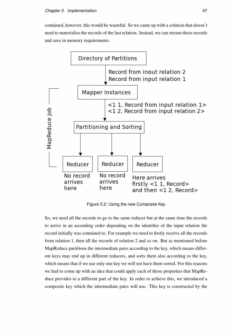
Chapter 5. Implementation 47
contained, however, this would be wasteful. So we came up with a solution that doesn’t
need to materialise the records of the last relation. Instead, we can stream these records
and save in memory requirements.
Figure 5.2: Using the new Composite Key
So, we need all the records to go to the same reducer but at the same time the records
to arrive in an ascending order depending on the identifier of the input relation the
record initially was contained to. For example we need to firstly receive all the records
from relation 1, then all the records of relation 2 and so on. But as mentioned before
MapReduce partitions the intermediate pairs according to the key, which means differ-
ent keys may end up in different reducers, and sorts them also according to the key,
which means that if we use only one key we will not have them sorted. For this reasons
we had to come up with an idea that could apply each of those properties that MapRe-
duce provides to a different part of the key. In order to achieve this, we introduced a
composite key which the intermediate pairs will use. This key is constructed by the

Chapter 5. Implementation 48
mapper instances. Then, we extended the Partitioner and WritableComparator classes
so that we can apply each of the two functionalities to the appropriate part of the key
so that both of the above mentioned requirements are guaranteed.
As mentioned to the previous section, after the partitioning phase ends, the produced
partitions are moved to new files that are given as input paths to the jobs that will
execute the join part of the algorithm. In each of those files there will be the respective
partitions of all the input relations. For example in one file the first partitions of all
the input relations will be contained. Each partition is named in a way that determines
the input relation it was a part of. During the processing by the mapper, we can find
the name of the file that each record that reaches the mapper belonged to. This can
be achieved using the getPath() and getName() methods of FileSplit class. During
the processing in the reducer we cannot access these parameters, so since the actual
join processing is held out in the reducer, we should move this information from the
mapper to the reducer. So, we have extended the Mapper class in order to implement
the functionality needed. The map() method of the Mapper class has been overridden
for this reason. The map() method is called once for each record that reaches the
mapper instance. For each record, the name of the file that the record was taken from
is retrieved. Then a composite key is created in order to be used as the key of the
intermediate pair. The first part of the key is always the constant number 1. Then a
white space character is inserted, which is used as a delimiter. The second part of the
key would be a number that represents the input relation that the current record was
initially part of. For example if the record was initially contained in the second input
relation, the number 2 will be used as the second part of the key. Finally, a key-value
pair is emitted. The key of the pair is the above mentioned composite key. The value of
the pair is the whole record. By using this intermediate pair we achieve two properties.
Firstly, the information regarding the input file that each record was taken from is
preserved and forwarded to the reducer that the actual join will be executed. Secondly,
the two requirements mentioned before will be guaranteed using this composite key.
We have presented the way that the mapper creates the intermediate key-value pairs
it emits. We have also presented the structure of the composite key. As mentioned
before, we want all the records to be processed by the same process. So all the records
should end up in the same reducer, as it is the process that carries out the join operation.
Additionally, we want the records to be sorted in an ascending order regarding the input
relation they were contained. In order to achieve this, we should determine the reduce

Chapter 5. Implementation 49
function that a record will be processed by, using the first part of the key. The first part
of the key is constant for every record, so every record will end up in the same reduce
instance. Additionally, we want the sorting to be held out using the second part of the
key which determines the input file that the record was taken from. In order to achieve
these functionalities we extended the Partitioner and WritableComparator classes and
embedded new functionalities in them. The Partitioner class is the one responsible for
assigning intermediate key-value pairs to the reducer instances. The default Partitioner
examines the whole key in order to assign the pair to a reducer. The behaviour of the
new Partitioner class, we have created, is to examine only the first part of the key in
order to assign the key-value pair to a reducer for processing. The first part of the key
is constant for all records. Additionally, the functionality of the WritableComparator
class has been overridden. The WritableComparator class is the one responsible for
comparing two keys during the sorting of the intermediate key-value pairs. The default
functionality of the class is to compare two keys using the whole portion of them.
We have overridden this functionality. The new functionality is to compare two keys
by comparing the second part of them. So, the intermediate key-value pairs will be
sorted using the second part of the key which represents the input relation the record
was initially part of. An example of the way that the new composite key is used, is
presented in Figure 5.2.
So far, we have presented the way we use in order to guarantee the needed proper-
ties for the join part of the algorithm. We have extended the Mapper, Partitioner and
WritableComparator classes and overridden their default functionalities. With this im-
plementation we guarantee that: firstly, the information regarding which input relation
each record came from will be preserved and forwarded to the reducer instances; sec-
ondly, all the records will end up to the same reducer instance; finally, the records will
be sorted according to the input relation they came from. So the actual join process is
ready to be executed. In the rest of this section we explain the implementation of the
join process by the reducers.
5.2.2 Simple Hash Join and Parallel Partitioning Hash Join
The join processing of Simple Hash Join and Parallel Partitioning Hash Join is quite a
simple process. These two algorithms receive as input two relations and execute a join
operation on them. An in-memory join has to be carried out between the records of the

Chapter 5. Implementation 50
two input relations. All we have to do is: firstly, insert the records of the first relation
in a hash table using the join attribute as the key; secondly, probe the records of the
second relation through the hash table; finally, export all the matching records of the
two relations.
In order to execute the above mentioned functionality we need a way to retrieve the
join attribute of every record that comes for processing depending on the input relation
that the record was initially a part of. As we have previously mentioned this informa-
tion was assigned to the instance of the Context class that was used by the partitioning
phase of the algorithm. We also need this information to be distributed in every one
of the reducer instances that will carry out the in-memory join of the records. So, we
extend the Reducer class in order to implement a new functionality that will execute
the join phase of the algorithm. The setup() method of the Reducer class is overrid-
den. The setup() method is called once before the first intermediate key reaches the
reducer instance. The new functionality of the setup() method is to use the instance of
the Context class in order to retrieve the Configuration instance using the getConfig-
uration() method of the Context class. Then, using the get() and getInt() methods of
the Configuration class, the positions of the join attributes within each relation can be
retrieved and initialised. Now the information is available for use during the execution
of the reduce phase. In order to implement a new functionality in the reduce phase of
our job, we override the reduce() method of the Reducer class. The reduce() method
of the reducer is called once for every key and set of values associated with the key
that arrives at the particular reduce instance. For only two inputs, the functionality of
the reduce() method is trivial. Considering the fact that the records come sorted (and
grouped), it is easy to identify that the process is quite simple. Firstly, all the records
of the first input relation will reach the reducer. These records will be inserted in a
hash map. The join attribute will be used as the key of the hash map. Subsequently,
all the records of the second input will reach the reducer. These records will be probed
through the hash map that has been already constructed. If a matching record of the
first relation is found, then a new record will be created. The new record will con-
tain the join attribute once and the two records of the input relations without the join
attribute. The new record is then exported.
We have already explained the functionality that the MapReduce classes will imple-
ment within the MapReduce job. But how will this MapReduce job contribute to the
overall data-flow of our system? We want to execute the join phase of our algorithm

Chapter 5. Implementation 51
Figure 5.3: Data-flow of the system for two input relations
in parallel. However, as mentioned before, all the records should be processed by the
same reducer instance. So, the parallelism that MapReduce offers cannot be exploited.
The map instances of the jobs used will run in parallel, but all the records will be pro-
cessed by the same reduce instance. In order to make this phase of our system parallel,
many MapReduce jobs will be used. We want to join every set of partition in paral-

Chapter 5. Implementation 52
lel. So, we will use as many jobs as the partitions created. Each of those jobs will be
initialised using the Configuration instance mentioned before, so the information that
is assigned to it is distributed to all the mapper and reducer instances that are used by
the job. The above mentioned Mapper and Reduce classes will be set for the jobs us-
ing the setMapperClass() and setReducerClass() methods of Job class. The Partitioner
that the jobs use is the one mentioned before. This will be set using the setPartition-
erClass() method of the Job class. Additionally the comparator that will be used for
the sorting phase of the algorithm, will also be the mentioned one. This is set using
the setSortComparatorClass() method of the Job class. In the previous subsection we
had mentioned that after the partitioning stage, new directories will be created and the
respective output files of the previous MapReduce jobs will be moved there in order
to be set as the input paths of the MapReduce jobs that will execute the in-memory
join. So there has been a new directory created for every partition that is used. In
every such directory there exists one file for every input relation. We want to join the
files of each such directory in parallel. So, each such directory will be given as the
input path for one of the join jobs. In order to accomplish this, the addInputPath()
method of FileInputFormat class will be used. Additionally, one new directory will be
used as output path for every one of the join jobs. This will be accomplished using
the setOutputPath() method of the FileOutputFormat class. Each of the directories that
are created and used as outputs of the jobs will contain as many files as the number
of reducers used for the job. However, all the files except of one will be empty. The
only non empty file will be the one of the reducer that executed the in-memory join.
This file will contain the actual results of the join. Finally, the jobs are submitted to the
cluster using the submit() method of the Job class. This method submits the MapRe-
duce job to the cluster and returns immediately. Subsequently the jobs are checked, in
order to verify that they have been successfully finished, using the isComplete() and
isSuccessful() methods of the Job class. The whole data-flow of the system, which was
just described, is presented in Figure 5.3.
5.2.3 Multiple Inputs Hash Join
Multiple Inputs Hash Join is the most generic version of parallel Hash Join. It receives
an arbitrary number of input relations and it executes the join operation on them. The
in-memory join algorithm that is executed is a little more complicated than the one we
described before for the other two algorithms that receive only two input relations in

Chapter 5. Implementation 53
order to execute the join. He have described above the way that the Mapper class is im-
plemented. Additionally, the way that the intermediate key-value pairs are partitioned
and sorted was described.
In order to execute the in-memory join algorithm, we need a way to retrieve the join
attribute of every record that comes for processing, depending on the input relation
that the record was originally a part of. As mentioned before, this information was
assigned to the instance of the Context class that was used by the partitioning phase of
the algorithm. We also need this information to be distributed in every reducer that will
execute the in-memory join of the records. So, we extend the Reducer class in order
to implement a new functionality that will execute the join phase of the algorithm.
The setup() method of the Reducer class is overridden. The setup() method is called
once before the fist record reaches the reducer instance. The new functionality of the
setup() method is to initialise the positions of the join attributes within the records of
each relation using the get() and getInt() methods of the Configuration class. Now the
information is available during the execution of the reduce phase.
After the partitions of the input relations have been assigned to reducers and sorted,
the intermediate key-value pairs will reach the reducer instances, at which the actual
join operation will be executed. One reduce instance will be used in which the records
will arrive ordered and grouped by the file identifier. As mentioned before, if we
were implementing the textbook algorithm, we should create N-1 hash tables using the
records of the first N-1 input relations and then probe the records of the last relation
through every hash table sequentially. However this algorithm would require a huge
memory footprint. In order to minimise the amount of memory that the in-memory
join requires, we have used an algorithm that during its execution uses only one hash
table and at most two lists. The first list is called previous-list and the other one next-
list. Firstly, the records of the first input relation will reach the reducer and will be
inserted into previous-list. For every relation that will arrive after this, a hash table
will be constructed using its records and the previous-list will be probed through it
storing the matching records in the next-list. At the end of every round the contents
of next-list will be moved to previous-list. When the final input relation arrives, the
same algorithm will be used except that the matching records will now be exported.
The new records that will be exported will contain the join attribute once and then all
the records of the input relations without the join attribute. If at some point during the
execution, the previous-list is empty, then the execution stops as the result of the join

Chapter 5. Implementation 54
that has been executed so far is the empty set. So, the result of the whole join would be
the empty set. Additionally, if the partition of one input relation is empty, the execution
also stops as the join result of the specific partitions would be the empty set.
The MapReduce jobs used in order to implement the join phase of the algorithm are
configured exactly in the same way as the ones used for the join phase of the two previ-
ous algorithms. We use one MapReduce job for each partition. The only difference is
that the input path of the jobs may contain more than two files that represent partitions
depending on the number of input relations. However, this doesn’t affect the rest of the
previously used data-flow of our system.
5.3 Merging phase
The last phase of the Parallel Hash Join algorithm is the merge phase. The in-memory
joins have already been executed. Now the results of all the parallel joins should be
merged in order to accumulate the final result of the algorithm. The first idea was to use
another MapReduce job for the merging of the results of the parallel joins. However
such an action would produce additional overhead to our system. We used a more
efficient technique that uses the HDFS in order to implement the merging phase of the
algorithm. Using HDFS commands, the files are moved into one directory and then
they are merged. At the end all the intermediate directories and files that have been
created during the execution are deleted.
After the join phase of our algorithm, there will be as many directories as the partitions
used. These are the output directories of all the MapReduce jobs that executed the
in-memory joins. In every one of those directories all the files will be empty except
of one that contains the results of the join. This is a result of the use of one reducer
instance for the implementation of the join part. We want to merge the contents of all
the partitions. So, we want to merge the contents of all the directories created by the
join processes. Within each such directory, we also want to merge all the files. The
non-empty file contains the actual results and the empty files will not have any effect
on the result.
So, a new directory is created using the mkdirds() method of FileSystem class and all
the files of all the partitions are moved there using the rename() method. Finally, all
the files of the new directory are merged and moved to the local file system using the

Chapter 5. Implementation 55
copyMerge() method of FileUtil class. At this point, we have the final result of the join.
However we want the results to be on HDFS for further processing by other MapRe-
duce jobs. Using the moveFromLocalFile method of FileSystem class, we move the
files back to HDFS. The result of the join is ready and back on HDFS.

Chapter 6
Evaluation
In previous chapters we have presented the functionality of the system we have im-
plemented. The data-flow of the system has been presented and explained. Addition-
ally, the technique used in order to apply query evaluation algorithms that are used by
Parallel DBMSs on Hadoop MapReduce framework were presented. Moreover, the
implementation of our system was presented and explained from a more technical as-
pect. The classes extended in order to embed the demanded functionality in our system
were presented as well as the way that the new functionality of the classes contributes
in the overall data-flow of the system. As mentioned in previous chapters, our system
focuses in evaluating the Join operator, as it is the most commonly used operator. For
this reason, the Join operator is also the most optimised one. In more detail, we focus
on Hash Join operator as it is the most parallelisable join operator. Three versions of
parallel Hash Join algorithms have been developed: firstly, Simple Hash Join, which
is the implementation of the textbook parallel Hash Join algorithm; secondly, Parallel
Partitioning Hash Join, which is an optimisation of Simple Hash Join; finally, Multiple
Inputs Hash Join which is the most generic algorithm that can execute a join operation
on an arbitrary number of input relations.
After the system was designed and implemented, we carried out experiments in order
to verify the efficiency of our system and its performance under various scenarios.
During each one of those scenarios some variables were kept constant and different
values were assigned to other ones. With this technique we intended to isolate the
variation of a specific variable and identify the impact that this variation has to the
overall performance of the system. Additionally, we carried out experiments using our
56

Chapter 6. Evaluation 57
algorithms and the algorithms that are typically used on MapReduce framework for
join evaluation, in order to compare their performance. This chapter presents the whole
evaluation process that was followed. The chapter is organised as follows: firstly,
the metrics that were used in order to measure the performance of the algorithms are
presented; secondly, the scenarios for which the algorithms were tested are presented;
furthermore, the performance that the algorithms were expected to have is presented;
finally, the results of the testing process are presented and some characteristics of the
algorithms are discussed.
6.1 Metrics
In this section, the metrics that were used in order to evaluate the performance of
the algorithms are presented. The quantity we use in order to measure and compare
efficiency, is time. As was mentioned in previous chapters, the time is reported at
crucial parts of the code which allows us to measure and compare the performance of
the algorithms, as well as the performance of the parts that the algorithms consists of.
The time is reported in six points during the execution of the algorithm:
1. Before the execution of the algorithm begins.
2. After partitioning the input relations and before starting joining the partitions.
3. After joining the partitions in parallel and before starting merging the interme-
diate results.
4. After merging the intermediate results and moving them to the local file system.
5. After moving the final results back to HDFS.
6. After the algorithm has been completed.
Reporting these times is crucial for our evaluation as they allow us to compute the
exact amount of time that was needed in order to be executed different parts of the
algorithm. Using these times we can compute the exact time that was needed in order
to execute the partitioning stage of each parallel Hash Join algorithm. Additionally, we
can compute the exact time that was needed in order to execute the parallel join on the
partitions. We can also compute the time that was needed for merging the files and for
moving them to the local file system of the user. Moreover, we can compute the time

Chapter 6. Evaluation 58
that was needed in order to move the files back to HDFS.
When the third time is reported, the join evaluation has finished. At this point, there
is a directory on HDFS called combined unmerged which contains a number of files
equal to the number of partitions that were used for the execution of the join operation.
Each of those files contains the result of the join operation that was applied between
the respective partitions. The merging of these files provides the total result of the
evaluation of the join operation between the input relations. Typically, a join algorithm
that runs in Hadoop MapReduce, would stop the evaluation of the algorithm right here,
leaving on HDFS a certain directory which contains the result of the join not necessar-
ily merged. This is because, usually an application running on Hadoop MapReduce,
does not execute only one MapReduce job. It executes a data-flow which consists of
multiple MapReduce jobs some of which receive as input the outputs of others. So
if we want one job to receive as input the result of the previously executed join, we
just have to use as input path of the job the above mentioned directory under which all
the results of the joins executed on the partitions are placed. In this way the existing
algorithms for join evaluation on MapReduce, Map-side and Reduce-side join, place
their results on HDFS. They do not create a file which contains all the results but a
directory on HDFS under which there are multiple files which contain the results.
However, for our algorithms we have also implemented the merging part. This part
was implemented mainly for completeness, as a parallel join algorithm executed by a
DBMS would do so. Typically, a parallel DBMS, during the merging phase, collects
all the parts of the parallel executed steps and merges them into one file. In order to
implement this part, all the files under the above mentioned directory are moved to
the local file system and then moved again on HDFS. The last two steps add a huge
overhead to our system, because moving files between the local file system and HDFS
is a time consuming operation. Unfortunately, the time consumed by the merging part
cannot be decreased.
As we have already explained the join algorithms executed on MapReduce, do not
merge their result as there is a much more efficient way for MapReduce jobs to pro-
cess join results. Additionally, the huge and inevitable overhead caused by the the
merging phase makes clear that this phase does not offer anything to our system but
adds overhead. So, although we have implemented this phase, we did not use it during
the evaluation of our algorithms, as a typical MapReduce join algorithm would do. In
order to evaluate the quality of our algorithms, we use the time quantity that was con-

Chapter 6. Evaluation 59
sumed until the results of the parallel in-memory joins are under combined unmerged
directory on HDFS. This time is mentioned as the turnaround time of the algorithm.
Additionally the time that the partitioning phase consumed and the time that the join-
ing phase consumed are two quantities that were taken into consideration in order to
evaluate the efficiency of the algorithms under different scenarios.
6.2 Evaluation Scenarios
In this section we present the scenarios we used in order to carry out the evaluation pro-
cess of our algorithms. Firstly, we are giving a short overview of the Hadoop cluster
that was used for the testing of the evaluation process as well as some of its character-
istics that had an impact on the scenarios we created. In order to test the performance
of the implemented algorithms, we used the Hadoop cluster provided by the university.
The cluster consists of 70 nodes, 68 of which were available during the execution of
the experiments. Additionally, the cluster provides Map Task and Reduce Task capac-
ities equal to 120 instances. It is worth mentioning that this limitation decreased the
performance of our algorithms, since during the execution of our experiments other
users were also using the cluster. So, if the number of Map or Reduce instances used
at a specific time, reaches the maximum allowed number, then any extra map instances
have to wait until one of the execution slots that were in use, becomes free. This sit-
uation limits the performance of our system and leads to sequential execution of parts
of code that should be executed in parallel, as some of the map or reduce instances
have to wait until resources are released. So, the time quantities that are reported in
latter parts of the chapter may be larger that the actual time quantity that our system
would report in the optimal case. Another aspect that formed a limitation to the testing
process, is the available memory that the nodes of the cluster provide to the reduce and
map instances. The in-memory join which is executed during the joining part of our
algorithm needs a certain amount of memory in order to store the hash table and the
lists used. In order to be able to process larger quantities of data, we have to use a
greater number number of partitions to add parallelism to the process and avoid run-
ning out of available memory. However, the provided cluster sets a limitation in the
number of partitions that can be used. During our evaluation process we could use a
maximum number of 100 partitions. The two latter characteristics of the cluster set a
limit to the size of datasets that can be processed, since the size of available memory of

Chapter 6. Evaluation 60
the processes as well as the number of partitions used could not exceed a certain limit.
We now present the scenarios that were used in order to carry out the evaluation pro-
cess. In every case we tried to isolate one of the variables and change it in order to
define the variation in performance regarding the specific variable. In order to create
the input relations, a random generator was used. Each file created by the generator
contains sixteen attributes. Some of them contain unique values which are included
only once in the column of the relation. The type of join that is executed is the same
for all the scenarios. Each time we join two or more relations of the same size using
one of the columns that contain the unique values as the join keys. By applying this
kind of join operation on two input relations we receive a relation consisting of the
same number of records as the input relations, since we use the columns that include
the unique values as the join attributes, and with almost double the size of the one of
the input relations, since the records of the result relation are the concatenation of the
records of the input relations with the join attribute included only once. In case of
joining three input relations, we acquire an output relation with the same number of
records but almost triple the size of the input relations. We keep the association be-
tween the input relations constant so that there are no variations in the results because
of it. Additionally, since the results can be estimated depending on the input relations,
we can verify the correctness of the result by just checking the size and the number of
records of the result relation and compare them with the size and the number of records
of the input relations.
In order to carry out the evaluation process, we used three datasets. Every dataset
consisted of files of a specific size. The datasets consisted of files of size equal to
one, two and three gigabytes. During the evaluation process, we conducted two sets
of experiments. Firstly, we wanted to compare the performance of the algorithm we
designed and implemented to the performance of the algorithms that are typically used
for join evaluation on MapReduce. Secondly, we wanted to evaluate the performance
and the efficiency of the algorithms we implemented under different scenarios.
The first set of experiments had as a goal to compare the performance of the algorithms
that are traditionally used in order to evaluate joins on MapReduce to the performance
of our algorithms. When we want to evaluate a join operation on MapReduce, we use
a Map-side, Reduce-side or in-memory join. We did not test in-memory join as there
are special requirements, on the size of the input relations, that should be satisfied in
order to use it. We used the Map-side and Reduce-side joins in order to compare their

Chapter 6. Evaluation 61
performance with the performance of our algorithm. In order to make the comparison,
we used the best available edition of our algorithm for two inputs, Parallel Partitioning
Hash Join. We executed the join operation using all the above mentioned algorithms
and then compared the results. We also applied the algorithm on input relations of
different sizes in order to define the variation in performance as the input grows.
The second set of experiments had as a goal to evaluate the performance of the im-
plemented algorithms under different scenarios. Firstly, we wanted to evaluate the
difference in performance between Parallel Partitioning Hash Join and Simple Hash
Join. In order to demonstrate the improvement in performance provided by the first
one, we applied both in the same set of data. In order to emphasise the enlargement
of the performance difference as the input grows, we applied the two algorithms on
inputs of different sizes. Secondly, we wanted to evaluate the improvement in the per-
formance of the algorithm as the number of partitions used grows. In order to achieve
this, we applied the same algorithms on the same datasets changing the number of par-
titions that were used. We also used multiple datasets in order to find how the boost in
efficiency provided by increasing the number of partitions changes as the size of the
input data grows. Finally, we wanted to evaluate the efficiency which is provided by
Multiple Inputs Hash Join. The alternative way to join three input relations, is by join-
ing the first two relations and then joining the result with the third one. We compared
the difference in performance of those two techniques. This was achieved by executing
a join between the same input relations using Multiple Inputs Hash Join algorithm and
also multiple Parallel Partitioning Hash Join algorithms. We carried out the tests using
datasets of different sizes in order to demonstrate the difference in performance as the
size of the input relations grows.
It is worth mentioning that, in order to achieve a greater level of accuracy, for each
one of the above mentioned tests, we executed the algorithms multiple times in order
to compute an average execution time. Thus, any possible variations in performance
that were caused by the change of available resources of the Hadoop cluster, were
normalised. The execution times reported later in this chapter are the average execution
time of five executions of each algorithm.

Chapter 6. Evaluation 62
6.3 Expected Performance
In the previous section, we presented the scenarios that are used in order to evaluate the
performance of our algorithms. As was mentioned before, the evaluation process has
two goals: firstly, to compare the performance of our algorithms with the performance
of the algorithms typically used for join evaluation on MapReduce; secondly, to evalu-
ate the performance of our algorithms under different scenarios. Before executing the
actual tests, in this section, we present some predictions about the performance of our
algorithms. After the tests were executed, the actual performance of out algorithms
was compared to our predictions.
Firstly, as mentioned before, our algorithm is compared to the typical algorithms that
are used for join evaluation on MapReduce framework. In order to carry out this com-
parison we use the most efficient version of parallel Hash Join for two inputs, Parallel
Partitioning Hash Join. We expect our algorithm to outperform both, the Map-side
and Reduce-side, join algorithms. However, Map-side join requires a sorted and parti-
tioned input in order to execute the join operation. Since we want the join algorithms
to be generic we include the time needed for sorting and partitioning the input in the
turnaround time of Map-side join. So, the data-flow used to implement Map-side join
sorts and partitions the input relations before starting the MapReduce job. Then, the
join is executed during the map phase of the job. On the other hand, Reduce-side join
firstly tags the records of the input relations with an identifier that determines the rela-
tion in which each record was initially contained and then it executes the actual join.
We expect the performance of the Reduce-side join to be closer to the performance
of our algorithm than the one of Map-side join. The reason for this assumption is the
overhead that is added to Map-side join from the sorting and the partitioning of the
input. Additionally, we expect as the size of the input relations grows, the difference
in the performance between our algorithm and the typical MapReduce join algorithms
also to grow.
Secondly, the performance of our algorithms under different scenarios is evaluated. We
intend to alter one of the variables every time while keeping every other constant. In
this way, we can distinguish the affect that the change of the specific variable has to the
performance of the system. The first experiment of this set has as a goal to demonstrate
the difference in performance between Parallel Partitioning Hash Join and Simple Hash
Join. We expect Parallel Partitioning Hash Join to offer improved performance in any

Chapter 6. Evaluation 63
case. The difference of those two algorithms is the way that the partitioning phase
of the algorithm is executed. In Simple Hash Join it is executed in sequence while in
Parallel Partitioning Hash Join it is executed in parallel. So as input data grow larger,
the difference between the performance of the two algorithms is expected also to grow.
Since, as already mentioned, the input relations that are joined have equal size, the
partitioning phase of the Parallel Partitioning Hash Join algorithm should need almost
half the time that the partitioning phase of Simple Hash Join algorithm needs. As the
size of the input files grows larger, this difference should also increase. The second
experiment of this set has as a goal to define the improvement in efficiency as the
number of partitions used increases. When we increase the number of partitions used
by the algorithm, we also increase the parallelism that is achieved by our system. Thus,
we split our data into more partitions and execute the processing on every one of those
partitions in parallel. The performance of our system should improve proportionally
to the number of partitions. This should be much more distinguishable as data grow
larger. The last experiment of this set, focuses on the execution of the join operation
on multiple input relations. We use three input relations for this experiment. Firstly,
we join the three input relations using Multiple Inputs Hash Join. Then, we use two
binary joins in order to join the relations. The difference in performance is expected
to be rather big. By using Multiple inputs Hash Join, we execute all the parts of the
algorithm once. By using two Parallel Partitioning Hash Join algorithms, we execute
all the parts of the algorithm twice. Although the execution process of the join part
of Multiple Inputs Hash Join is the same with executing sequentially the join parts of
the two binary join algorithms, the overheads of all the other parts of the algorithm as
well as the overhead of initialising a MapReduce job, should cause a great increase in
the time that is consumed in order to execute the join using two binary join algorithms
instead of Multiple Inputs Hash Join.
6.4 Results
In previous sections we presented the scenarios used in order to test out algorithms un-
der different circumstances. Using these, we wanted to identify the effect that changes
in the variables of the system have to the performance of our algorithms. We have
already presented the metrics used in order to measure the efficiency and the perfor-
mance of our system. In this sections we present the results of our experiments and

Chapter 6. Evaluation 64
compare them with the above mentioned expected results. All the timings that are pre-
sented in this section represent the average seconds that each algorithm consumes in
order to be executed.
Parallel Partition-
ing Hash Join
Map-side Join Reduce-side Join
Execution Time -
1 GB
158 312 182
Execution Time -
2 GB
270 525 295
Execution Time -
3 GB
389 682 418
Table 6.1: Parallel Hash Join and traditional MapReduce Join evaluation algorithms (in
seconds)
Figure 6.1: Comparison between parallel Hash Join and typical join algorithms of
MapReduce
The goal of our first experiment was to compare the developed algorithm with the ones
that are typically used for join evaluation on MapReduce framework. In order to carry
out the comparison we used Parallel Partitioning Hash Join and also the algorithms
typically used by MapReduce framework for join evaluation, Map-side and Reduce-
side join. The results are reported in Table 6.1 and presented in Figure 6.1. The results

Chapter 6. Evaluation 65
Simple
Hash
Join - 1
GB
Parallel
Partition-
ing Hash
Join - 1
GB
Simple
Hash
Join - 2
GB
Parallel
Partition-
ing Hash
Join - 2
GB
Simple
Hash
Join - 3
GB
Parallel
Partition-
ing Hash
Join - 3
GB
Partitioning
Phase - 50
Partitions
168 85 213 134 360 241
Joining
Phase - 50
Partitions
127 120 183 174 678 660
Turnaround
Time - 50
Partitions
295 205 396 308 1038 901
Partitioning
Phase - 75
Partitions
151 73 207 128 437 256
Joining
Phase - 75
Partitions
107 98 162 160 311 283
Turnaround
Time - 75
Partitions
258 171 369 288 748 539
Partitioning
Phase - 100
Partitions
120 71 204 130 387 225
Joining
Phase - 100
Partitions
94 87 144 150 207 164
Turnaround
Time - 100
Partitions
214 158 348 270 594 389
Table 6.2: Simple Hash Join and Parallel Partitioning Hash Join (in seconds)

Chapter 6. Evaluation 66
Multiple
Inputs
Hash
Join - 1
GB
Multiple
Binary
Joins - 1
GB
Multiple
Inputs
Hash
Join - 2
GB
Multiple
Binary
Joins - 2
GB
Multiple
Inputs
Hash
Join - 3
GB
Multiple
Binary
Joins -
3GB
Partitioning
Phase - 75
Partitions
111 - 203 - - -
Joining
Phase - 75
Partitions
117 - 230 - - -
Turnaround
Time - 75
Partitions
228 437 433 738 - -
Partitioning
Phase - 100
Partitions
118 - 210 - 314 -
Joining
Phase - 100
Partitions
101 - 189 - 378 -
Turnaround
Time - 100
Partitions
219 408 399 652 692 904
Table 6.3: Multiple Inputs Hash Join and multiple Binary Joins (in seconds)
from the experiments were quite similar to the expected ones. Our algorithm outper-
formed both of the typical MapReduce algorithms. Moreover, as was expected, the
performance of Reduce-side join was closer to the performance of our algorithm than
the one of Map-side join. This is reasonable, as the overhead that is added to Map-side
join from the sorting and partitioning that has to be carried out before the execution
of the actual join is huge. As is presented in Figure 6.1 our algorithm outperforms
Map-side join by a long distance but is really close to the performance of Reduce-side
join. The lines that indicate the performance of Parallel Partitioning Hash Join and
Reduce-side join seem to be almost parallel. However, by carefully considering Table

Chapter 6. Evaluation 67
6.1, someone can observe that our algorithm doesn’t only outperform the traditional
algorithms used by MapReduce for join evaluation, but also the difference in perfor-
mance increases as the size of the input files gets larger. So, the scalability provided by
our system overcomes the scalability that is provided by the typical MapReduce join
algorithms.
Furthermore we wanted to evaluate the performance of the developed algorithm under
different scenarios. In order to demonstrate the characteristics of the algorithms we
changed the number of the partitions that are used as well as the number of the input
files that are joined. We executed a variety of experiments, the results of which are
reported in Tables 6.2 and 6.3 and also presented in Figures 6.2-6.8.
Figure 6.2: Comparison between Simple Hash Join and Parallel Partitioning Hash join
The first goal of this set of experiments, was to demonstrate the performance differ-
ence between Parallel Partitioning Hash Join and Simple Hash Join. We executed both
algorithms using input relations of different sizes and a variety of partitions. As is
demonstrated in Table 6.2 and also presented in Figures 6.2-6.4, in every case, as was
expected, Parallel Partitioning Hash Join outperformed Simple Hash Join. Further-
more, someone can notice, by observing carefully Figures 6.2-6.4, that the difference
in performance between the two above mentioned algorithms is increasing as the size
of the input relations is growing. As we can see, the two algorithms need almost the
same amount of time in order to execute the joining phase of the algorithm, if the

Chapter 6. Evaluation 68
Figure 6.3: Comparison between Simple Hash Join and Parallel Partitioning Hash join
same number of partitions is used. This is reasonable, as the two algorithms use the
same technique in order to implement the joining phase of the algorithm, as has been
presented in previous chapters. The difference in the execution times of the two al-
gorithms is caused by the difference in the execution times of the partitioning phase.
Parallel Partitioning is much more efficient, because the input relations are partitioned
in parallel instead of sequentially like Simple Hash Join. Consequently, the total time
consumed by the partitioning phase of Parallel Partitioning Hash Join is equal to the
time consumed for partitioning the largest input relation. On the other hand, Simple
Hash Join partitions the input relations in sequence, so the total time consumed for
the partitioning phase is equal to the sum of the times that are consumed for parti-
tioning each one of the input relations. This explains the increase in the performance
difference as the size of the input relations gets larger.
Since the two input relations have equal size, the time consumed by the partitioning
phase of Parallel Partitioning Hash Join should be almost half the time that is consumed
by the partitioning phase of Simple Hash Join. However this is not the case. This is
happening because the limitations of the provided cluster restrict our algorithms from
running in a fully parallel manner. As we have mentioned before, our cluster provides
us with a capacity of 120 reduce tasks. During the partitioning of the input relations
we need as many reducers as the partitions used. So, for 75 and 100 partitions, we need

Chapter 6. Evaluation 69
Figure 6.4: Comparison between Simple Hash Join and Parallel Partitioning Hash join
150 and 200 reduce tasks accordingly, which cannot be provided by the cluster. When
all the reduce slots are occupied, until some reduce instance finishes, some other will
wait for it to end in order to execute its functionality. As we can see, parts of the al-
gorithm that should be executed in parallel, are executed in sequence. We would need
a cluster with a larger reduce instances capacity, which would provide real parallelism
to our system, in order to achieve the time consumed for partitioning by Parallel Parti-
tioning hash join to be half the time that is consumed for partitioning by Simple Hash
Join.
The second goal of this set of experiments, was to demonstrate the improvement in ef-
ficiency as the number of partitions grows larger. In order to identify the performance
variance, we have executed the join operation multiple times, increasing the number of
partitions that are used for the process. Additionally, the size of the input relations is
increased, in order to observe how the improvement in efficiency changes as the size of
the input files increases. As it is demonstrated in Table 6.2 and also presented in Fig-
ures 6.5 and 6.6, the efficiency of the algorithm increases as the number of partitions
used grows larger. Furthermore, by observing carefully Figures 6.5 and 6.6, someone
can understand that as the size of the input relations gets larger, the difference in per-
formance provided by increasing the number of partitions increases as well. As we
can observe in Figures 6.5 and 6.6, the improvement offered by increasing the number

Chapter 6. Evaluation 70
Figure 6.5: Comparison of performance as number of partitions increases
of partitions, is way more significant when the input relations have size equal to three
gigabytes compared to the one that is observed when the input relations have size equal
to one or two gigabytes.
Figure 6.6: Comparison of performance as number of partitions increases
The above mentioned result was expected, as the increase in the number of partitions
used, has as a result the increase in the the parallelism of the system. The time con-
sumed by the partitioning phase is almost the same no matter how many partitions are

Chapter 6. Evaluation 71
used. However there is a distinguishable decrease in the time consumed by the joining
part of the algorithm, as the number of the partitions increases, which can be observed
in Table 6.2. This decrease results in the decrease of the overall time that is consumed
by the algorithm in order to execute the partition. The joining part of the algorithms
is carried out in parallel. Every parallel process executes an in-memory join between
two respective partitions of the two input relations. In our implementation, we use one
MapReduce job in order to execute every one of the parallel in-memory joins. When
the number of partitions grows, more MapReduce jobs are used in order to execute the
in-memory joins in parallel. The input data are split into more partitions which are
subsequently joined in parallel. As the size of the input files increases, splitting the
input relations in as many partitions as possible becomes much more important.
Figure 6.7: Comparison between Multiple Inputs Hash Join and multiple binary joins
The final goal of this set of experiments, was to demonstrate the increase in efficiency
by using Multiple Inputs Hash Join instead of multiple binary joins for executing a join
operation on more than two input relations. In order to demonstrate this characteristic
we used three input relations. As mentioned before there are two ways to execute a
join operation on three input relations. The first one is by using Multiple Inputs Hash
Join. The second one is by using Parallel Partitioning Hash Join twice: the first time
in order to execute the join between two of the three input relations; and the second
time in order to execute the join between the third relation and the result of the previ-
ous join operation. We used both techniques in order to compare their performance.

Chapter 6. Evaluation 72
Figure 6.8: Comparison between Multiple Inputs Hash Join and multiple binary joins
Additionally, we changed the size of the input relations in order to observe variations
in the difference between the two methods as the size of the input relations increases.
The results are reported in Table 6.3 and also presented in Figures 6.7 and 6.8. As we
can understand by observing the results, Multiple Inputs Hash Join always results in
better performance from using two binary joins in order to carry out the operation.
The above mentioned result was expected and we expect Multiple Inputs Hash Join
always to outperform the efficiency provided by multiple binary joins. By executing
two binary joins we waste time as we need to perform all the phases of the algorithms
twice. On the other hand by using Multiple Inputs Hash Join, we execute every phase
only once. Of course the phases of Multiple Inputs Hash Join consume more time than
the respective parts of each one of the two join operations that are executed during the
other solution. More specifically, The join phase that is executed by Multiple Inputs
Hash Join, is equal to executing sequentially the join phases of the two algorithms. In
both cases the join of the two relations is computed and then the third relation will be
probed through the result in order to find matching records. However, because of the
overhead added by having to execute every other phase twice, the overall performance
of Multiple Inputs Hash Join should always outperform the performance of the two
binary joins.

Chapter 7
Conclusion
Relational Databases are a mature technology that has accumulated decades of perfor-
mance tricks, from its usage in industry, and huge experience from research and evo-
lution. The decades of research have provided a huge optimisation in the techniques
used for query evaluation. With the addition of parallelism, the processing power of
Database Management Systems has significantly increased. In order to exploit this
processing power, the query evaluation techniques used so far, have been modified
in order to execute their functionality in parallel. Parallel Database Systems consist
one of the most successful applications of parallelism in computer systems. These are
some of the reasons that have led to the dominance of parallel DBMSs in the field of
large-scale data processing.
On the other hand, MapReduce is a relatively new programming model that has spread
widely during the last years. There are even scenarios during which companies aban-
doned the old systems, which were based on parallel DBMSs, in order to adopt a
MapReduce-based solution. This widespread use of MapReduce framework is a re-
sult of the useful characteristics that the framework offers to any system based on it.
MapReduce framework offers scalability, fault tolerance, and a great level of paral-
lelism.
The goal of this work was to combine the experience of the query evaluation techniques
used by DBMSs with the advantages offered by MapReduce framework. This was
accomplished by adapting the efficient algorithms used by parallel DBMSs for query
evaluation on Hadoop, which is an open source implementation of MapReduce. More
specifically, the way that parallel DBMSs evaluate the join operator was examined, as
73

Chapter 7. Conclusion 74
join is the most commonly used relational operator and as a result the most optimised
one.
7.1 Outcomes
In order to apply the above mentioned idea we focused on Hash Join. The main reason
is that Hash Join is one of the join operators that can be parallelised more successfully.
In order to apply the parallel Hash Join operators that DBMSs use on top of Hadoop
MapReduce framework, we had to alter the data-flow of the framework. We extended
the main classes, in order to implement new functionality. Additionally, we combined
many MapReduce jobs in order to create a data-flow that simulates the one that DBMSs
use for query evaluation.
We designed and implemented three algorithms that execute parallel Hash Join eval-
uation: Simple Hash Join, which is the implementation of the textbook parallel Hash
Join algorithm, Parallel Partitioning Hash Join which is an optimisation of Simple Hash
Join that partitions the input relations in parallel; Multiple Inputs Hash Join, which ex-
ecutes a join on an arbitrary number of input relations. After designing and implement-
ing these algorithms we carried out experimental evaluation in order to demonstrate the
difference in performance between the implemented algorithms and the algorithms that
are typically used for join evaluation on MapReduce framework. Additionally, through
the experimental evaluation we demonstrated the performance of the algorithm as the
variables of the system change. We demonstrated that the performance of the algorithm
improves greatly as the number of partitions grow. Additionally, we demonstrated the
improvement in performance that can be provided by using Parallel Partitioning Hash
join instead of Simple Hash Join. Finally, we demonstrated the efficiency that is pro-
vided by using Multiple Inputs Hash Join instead of multiple binary join operators in
order to compute the join on several input relations.
7.2 Challenges
During the design and implementation of our system, we faced a lot of challenges.
Firstly, the characteristics of MapReduce that were useful for our goals had to be ex-
ploited while the characteristics that were useless had to be discarded as they added

Chapter 7. Conclusion 75
only overhead to the overall performance.
During the execution of parallel Hash Join, the actual join is computed in parallel
by executing an in-memory Hash Join between the respective partitions of the input
relations. In order to accomplish that, all the records of the input relations should
be processed by the same reducer instance. However, MapReduce after the mapping
phase, distributes the intermediate key-value pairs to the reducers depending on the key
attribute of each pair. Additionally, we wanted the pairs to reach the reducer grouped
in order to avoid materialising all the relations. In order to guarantee both the above
mentioned specifications, we implemented secondary sorting. So, we used a composite
key that consisted of a constant, as the first part, and an identifier, that represented
the input relation of every record, as the second part. Subsequently, we executed the
partitioning using the first part of the key and the sorting using the second part of it.
Another challenge, concerned the use of HDFS. We needed to link a number of MapRe-
duce jobs in order to simulate the data-flow of parallel DBMSs. In order to link the
jobs we had to modify and move the intermediate files in order to achieve, the output
files of a first set of jobs to be used as input files for another set of jobs. In order to ac-
complish this we needed to use the HDFS. So, we used the HDFS commands provided
by HDFS Api in order to execute efficiently those manipulations on the intermediate
files.
Moreover, during the execution of the join operation between an arbitrary number of
files, we had to compute an in-memory join between all the inputs. Of course this
operation has huge memory requirements if we use the textbook algorithm, as a hash
table of every input relation has to be stored in memory. In order to decrease the
likelihood of running out of memory, we implemented a new algorithm that during the
processing uses only one hash table and two lists to store the needed data. The records
are streamed and in any snapshot during the execution of the algorithm only the hash
table is materialised.
7.3 Future Work
Although we have made a step towards the direction of applying query evaluation
techniques that are used by parallel DBMSs on MapReduce framework, there is much
more work that has to be done. Firstly, one of the most important issues is the memory

Chapter 7. Conclusion 76
requirements of the algorithm. The second phase of the algorithm consists of execution
of in-memory joins in parallel between the respective partitions. We have already
mentioned that we have used an in-memory join algorithm that minimises the memory
requirements. However, this may not be enough as we have seen during the evaluation
part of this work. The obvious solution is to increase the parallelism of the system.
By splitting the input data into more partitions, we increase the likelihood of every
partition fitting into the available memory of every process. So, a kind of optimisation
technique should be developed that considers the size of the inputs and determines
the number of partitions that will be used so that the join can definitely be executed.
Additionally, during the in memory join it should define the order of the relations so
that the smaller one is materialised and the larger is only streamed.
Moreover, the developed system only implements equalities. The performance of the
algorithm while evaluating equalities determines its quality. The performance of it
during the evaluation of inequalities is determined mainly by the size of the input files.
However, the implementation of the evaluation of inequalities is a trivial process.
Finally, the implementation of parallel Hash Join is only a first step. The experience
of the evaluation techniques of DBMSs can be also combined with the advantages of
MapReduce in cases of other parallel query evaluation operations. One of the potential
join operations that can be efficiently parallelised, and would benefit from the paral-
lelism that MapReduce offers, is Sort-merge join. This operator can be implemented
quite easily on top of MapReduce by altering the way of assigning the intermediate
key-value pairs to reducers. After sorting them the whole set should be split into equal
sets and assign each of those to a reducer.

Bibliography
[1] Pragmatic programming techniques. http://horicky.blogspot.com/2008/
11/hadoop-mapreduce-implementation.htm%l.
[2] Introduction to parallel programming and mapreduce. http://code.google.
com/edu/parallel/mapreduce-tutorial.html.
[3] Stratis D. Viglas. Lecture slides of extreme computing course - databases
and mapreduce. http://www.inf.ed.ac.uk/teaching/courses/exc/
lectures/dbmr.pdf.
[4] David DeWitt and Jim Gray. Parallel database systems: the future of high perfor-
mance database systems. Commun. ACM, 35:85–98, June 1992.
[5] Jeffrey Dean and Sanjay Ghemawat. Mapreduce: simplified data processing on
large clusters. Commun. ACM, 51:107–113, January 2008.
[6] Dawei Jiang, Beng Chin Ooi, Lei Shi, and Sai Wu. The performance of mapre-
duce: an in-depth study. Proc. VLDB Endow., 3:472–483, September 2010.
[7] Yu Xu, Pekka Kostamaa, Yan Qi, Jian Wen, and Kevin Keliang Zhao. A hadoop
based distributed loading approach to parallel data warehouses. In Proceedings of
the 2011 international conference on Management of data, SIGMOD ’11, pages
1091–1100, New York, NY, USA, 2011. ACM.
[8] Raghu Ramakrishnan and Johannes Gehrke. Database Management Systems.
McGraw-Hill, Inc., New York, NY, USA, 3 edition, 2003.
[9] Michael Stonebraker, Daniel Abadi, David J. DeWitt, Sam Madden, Erik Paul-
son, Andrew Pavlo, and Alexander Rasin. Mapreduce and parallel dbmss: friends
or foes? Commun. ACM, 53:64–71, January 2010.
77

Bibliography 78
[10] Dhruba Borthakur, Jonathan Gray, Joydeep Sen Sarma, Kannan Muthukkarup-
pan, Nicolas Spiegelberg, Hairong Kuang, Karthik Ranganathan, Dmytro
Molkov, Aravind Menon, Samuel Rash, Rodrigo Schmidt, and Amitanand Aiyer.
Apache hadoop goes realtime at facebook. In Proceedings of the 2011 interna-
tional conference on Management of data, SIGMOD ’11, pages 1071–1080, New
York, NY, USA, 2011. ACM.
[11] Jimmy Lin and Chris Dyer. Data-Intensive Text Processing with MapReduce.
Synthesis Lectures on Human Language Technologies. Morgan & Claypool Pub-
lishers, 2010.
[12] Apache hadoop homepage. http://hadoop.apache.org/.
[13] Tom White. Hadoop: The Definitive Guide. O’Reilly, first edition edition, june
2009.
[14] Api of hadoop. http://hadoop.apache.org/common/docs/current/api/.
[15] Jason Venner. Pro Hadoop (Expert’s Voice in Open Source). Apress, 2009.
[16] Goetz Graefe. Query evaluation techniques for large databases. ACM Comput.
Surv., 25:73–169, June 1993.
[17] M. Tamer Ozsu and Patrick Valduriez. Distributed and parallel database systems.
ACM Comput. Surv., 28:125–128, March 1996.
[18] Annita N. Wilschut, Jan Flokstra, and Peter M. G. Apers. Parallel evaluation
of multi-join queries. In Proceedings of the 1995 ACM SIGMOD international
conference on Management of data, SIGMOD ’95, pages 115–126, New York,
NY, USA, 1995. ACM.
[19] Anant Jhingran, Sriram Padmanabhan, and Ambuj Shatdal. Join query optimiza-
tion in parallel database systems, 1993.