Implementation of Indoor Positioning using …603894/FULLTEXT01.pdf · Implementation of Indoor Positioning using ... of indoor positioning like WIFI, ... to the level of ±30 cm

Implementation of Indoor Positioningusing IEEE802.15.4a (UWB)

BINYAM SHIFERAW HEYI

Master’s Degree ProjectStockholm, Sweden

XR-EE-LCN 2013:005

Implementation of Indoor Positioning using IEEE802.15.4a (UWB)

A Thesis submitted for partial fulfillment of the Masters of Science in Electrical Engineering Major in Network Services And Systems

AUTHOR:BINYAM SHIFERAW HEYI

January,2012 Stockholm, Sweden

KTH

The Royal Institute of Technology Laboratory for Communication Networks ,School of Electrical Engineering

SUPERVISORS:

PETER REIGO (MARNA TECH AB)

VIKTORIA FODOR (KTH)

EXAMINER:

VIKTORIA FODOR

2

Acknowledgements

I would like to thank Marna Tech AB for giving me the opportunity to carry out this thesis work under

their supervision. I would like to express my sincere gratitude and appreciation for my supervisor

Peter Reigo of Marna Tech AB for his constant support and encouragement. His excellent and

invaluable guidance has been instrumental in making this project work a success.

I would like to thank my supervisor Prof. Viktoria Fodor for her valuable comments and supports.

I would like to thank my family in Addis Ababa for their continuous support in my whole two year

study in Sweden.

Finally I would like to thank my friends Asmeret, and Nur who lived with me in the same corridor for

the last two years and provided me all the support that I needed.

Binyam Shiferaw Heyi

Stockholm,Sweden

January, 2013

3

Abstract

Indoor positioning is a technique that is used to locate a mobile device in indoor environment in real

or near real-time. The demand for indoor positioning system as a location based system is becoming

more and more widespread. However, the field has not gain much success as outdoor positioning

system.

The objective of this thesis work is to design and implement an indoor positioning system that relies

on ultra wide band technology. The report also describes the way how to implement IEEE802.15.4a

physical layer and medium access layer .The system uses time difference of arrivals technique to

estimate the position of the mobile device.

Through an evaluation of our system, we conclude that ranging can reach an accuracy of ±20cm in

line of sight measurement and ± 50cm for non-line of sight measurement. But the localization that is

achieved has an accuracy is up to ±1.1m, we believe this can be improved by having all device to be

synchronized effectively.

4

List of Figures

Figure 1:Bandwidth of 802.15.4a channels ....................................................................................... 16

Figure 2:UWB frame format .............................................................................................................. 17

Figure 3: UWB PHY signal flow .......................................................................................................... 17

Figure 4:UWB symbol format ............................................................................................................ 18

Figure 5:WSN node Architecture ....................................................................................................... 19

Figure 6: Sensor network architecture .............................................................................................. 20

Figure 7: SMAC operation ................................................................................................................ 22

Figure 8: BMAC operation ................................................................................................................ 23

Figure 9: DMAC operations .............................................................................................................. 23

Figure 10: TMAC operations ............................................................................................................. 24

Figure 11: LEACH operation. ............................................................................................................. 25

Figure 12: PEDAMACS operation ...................................................................................................... 26

Figure 13: Indoor Positioning Techniques ......................................................................................... 28

Figure 14: Ranging ............................................................................................................................ 29

Figure 15:Standard Ranging .............................................................................................................. 30

Figure 16: Private Ranging................................................................................................................. 31

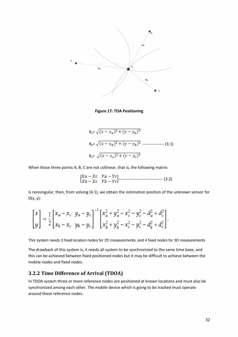
Figure 17: TOA Positioning ................................................................................................................ 32

Figure 18:TDOA Positioning............................................................................................................... 34

Figure 19: Overall System.................................................................................................................. 35

Figure 20: Hardware Structure .......................................................................................................... 36

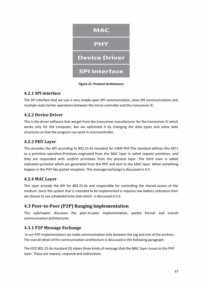
Figure 21: Protocol Architecture ....................................................................................................... 37

Figure 22: Sequence flow for two peer to peer message exchanges .................................................. 40

Figure 23: MAC Frame ...................................................................................................................... 41

Figure 24: Encoding format of the ranging Message .......................................................................... 42

Figure 25:P2P Ranging Implementation............................................................................................. 42

Figure 26: Encoding format of localization ........................................................................................ 45

Figure 27: Tag State Transitions ........................................................................................................ 46

5

Figure 28: Anchor state transition ..................................................................................................... 47

Figure 29:Coordinator state transitions ............................................................................................. 48

Figure 30:Synchronization ................................................................................................................. 50

Figure 31: TDOA transfer................................................................................................................... 51

Figure 32:Resynchronization ............................................................................................................. 52

6

List of Tables

Table 1 shows the 802.15.4a channel allocation. ............................................................................... 15

Table 2: Encoding Data Rate.............................................................................................................. 17

Table 3: Typical errors in synchronizations ........................................................................................ 34

Table 4: Message Exchange between PHY and MAC .......................................................................... 39

Table 5:Final Message Fields ............................................................................................................. 42

Table 6:Report Message Fields .......................................................................................................... 42

Table 7:P2P LOS measurement ......................................................................................................... 43

Table 8:P2P NLOS Measurements ..................................................................................................... 44

Table 9:localization Measurement Result .......................................................................................... 53

7

Abbreviations

WSN: Wireless Sensor Networks

UWB: Ultra-Wide Band

UWB IR: UWB impulse Radio

PHY: Physical

MAC: Media Access Control

TDOA: Time Difference of Arrival

TOA: Time of Arrivals

AOA: Angle of Arrival

RX: Receive

TX: Transmit

RSS: Receive Signal Strength

RFID: Radio Frequency Identification

WPAN: Wireless Personal Area Network

SHR: Synchronization Header

SPI: Serial Peripheral Interface

P2P: Peer-to-Peer Implementation

LOS: Line of Sight

NLOS: Non Line of Sight

8

Contents Acknowledgements ............................................................................................................................2

Abstract ..............................................................................................................................................3

List of Figures ......................................................................................................................................4

List of Tables .......................................................................................................................................6

Abbreviations .....................................................................................................................................7

1. Introduction .................................................................................................................................. 10

1.1 Problem Statement and Motivation ................................................................................... 10

1.2 Outline .............................................................................................................................. 11

2. Theory and Background ................................................................................................................ 12

2.1 Wireless Sensor Networks (WSN) ............................................................................................ 12

2.1.1 WSN Applications ............................................................................................................. 12

2.1.2 Wireless Personal Area Network (WPAN) ......................................................................... 12

2.1.3 Architecture of WSN ......................................................................................................... 19

2.2 Indoor Positioning Systems ..................................................................................................... 27

2.2.1 Infrared positioning systems ............................................................................................. 27

2.2.2. Optical positioning system ............................................................................................... 27

2.2.3 Radio frequency positioning system ................................................................................. 27

3. Ranging and Localization ............................................................................................................... 29

3.1Ranging .................................................................................................................................... 29

3.1.1Standard Ranging .............................................................................................................. 29

3.1.2Private Ranging ................................................................................................................. 30

3.2Localization .............................................................................................................................. 31

3.2.1 Time of arrivals (TOA) ....................................................................................................... 31

3.2.2 Time Difference of Arrival (TDOA) ..................................................................................... 32

4 Design and Implementation ........................................................................................................... 35

4.1 System Overview ..................................................................................................................... 35

4.1.1Hardware Components...................................................................................................... 36

9

4.2 Protocol Architecture .............................................................................................................. 36

4.2.1 SPI interface ..................................................................................................................... 37

4.2.2 Device Driver .................................................................................................................... 37

4.2.3 PHY Layer ......................................................................................................................... 37

4.2.4 MAC Layer ........................................................................................................................ 37

4.3 Peer-to-Peer (P2P) Ranging Implementation ........................................................................... 37

4.3.1 P2P Message Exchange ..................................................................................................... 37

4.3.2 Message Exchanged and Their Formats ............................................................................ 41

4.3.3 Discussion and Results of P2P implementation ................................................................. 42

4.4 Implementation of Localization ............................................................................................... 44

4.4.1 Message Exchanged for the localization ............................................................................ 44

4.4.2 State transition ................................................................................................................. 45

4.4.3 Media Access Control Design ............................................................................................ 48

4.4.4 Measurement Results ....................................................................................................... 52

5. Conclusion and Future Work ......................................................................................................... 54

5.1 Conclusion .............................................................................................................................. 54

5.2Future Work ............................................................................................................................. 54

Bibliography...................................................................................................................................... 56

10

1. Introduction

Asset tracking and wireless sensor networks are technologies of rapidly growing interest . During the

last years large companies and hospitals have drastically increased their operational efficiency by

using asset and people tracking systems. Imagine a hospital where you have very expensive

equipment that you easily share by having an online queue system and where you immediately can

find it when it is free. In the same system you can track demented patients to assure that they do not

get lost outside the hospital. Tracking of key personnel can also increase the overall efficiency. Thus

with these systems you can help organizations to drastically increase their output and reduce waste.

Wireless sensor network has also gained large interest the last years. Especially in large

manufacturing plants a large amount of parameters needs to be supervised. Up till now huge

investments needed to be done to install all wires to the different places where parameters need to

be supervised. The investment yielded that only the most important parameters were supervised.

Today it is possible to make wireless sensor networks where every sensor has a battery life of five

years and more. Because of the low installation cost of the wireless sensor network many more

parameters can be supervised and the output of the process can be further improved.

1.1 Problem Statement and Motivation

Global Positioning System (GSM) is used to locate people and assets in outdoor environment, but it

fails to repeat its success in indoor environment. Since satellites do not properly work in indoor

environment, indoor positioning relies on nodes in known location which actively locates people and

assets.

There are various ways of indoor positioning like WIFI, Bluetooth and UWB systems. The advantage of using UWB system is its fine time resolution, energy efficiency and robustness to interference in harsh environment. Due to UWB’s fine time resolution and by using very accurate ranging technique such as RSS (Receive Signal Strength), TDOA (Time Difference of Arrivals) or AOA (Angle of Arrivals) very precise measurement can be achieved. [15] The main objective of this thesis work is to design and implement a Physical (PHY) and Media Access Layer (MAC) according to the standard of IEEE802.15.4a UWB. With the goal to design and implement a very efficient indoor positioning system, where assets and

people can be tracked up to the level of ±30 cm and a battery life up to 3 years, we start our system

by implementing ranging in peer-to-peer system and then we expand our system to support four

station nodes with known location and a single movable node. In this system one of the nodes is

assigned to be a coordinator, which controls access to the shared medium. The rest of the nodes only

allowed to transmit or receive based on the slots assigned by the coordinator.

The choice of a good MAC layer protocol for WSN is an important factor for designing a good indoor

positioning system. In our implementation, we choose to implement a scheduled based MAC layer

protocol so as to reduce the idle listening power consumption of the node.

This master’s thesis contributes to knowledge area of the design and implementation of indoor

positioning by using UWB as a communication medium for WSN.

11

1.2 Outline

The thesis report is organized as follows:

Chapter 2 discusses the basic theory and background of WSN, WPAN, indoor positioning systems and

IEEE802.15.4a standard. Chapter 3 discusses the basics behind ranging and localization and how time

based localization can be implemented.Chapter 4 discusses our own design and implementation

including the hardware components, protocol architecture, peer-to-peer implementation and

localization implementation and the results we obtained. Chapter 5 discusses the conclusion and

recommendation for future work.

12

2. Theory and Background

This chapter discusses the overview of wireless sensor networks in general and IEEE 802.15.4a

standard starting from its definition, properties that distinguish it from other wireless sensor

protocols, modulation and demodulation techniques and channel allocations and available indoor

positioning techniques.

2.1 Wireless Sensor Networks (WSN)

A wireless sensor network contains a collection of several nodes which can able to sense the

environment they are deployed, communicate with each other or with other kinds of nodes and can

able to compute the data that they get from the environment. [9]

As the technology advances the nodes can able to communicate the wirelessly, and it is clear that the

sensors deployed should also be small size, low power, low cost, multifunctional and capable of

handling computation(software, hardware and algorithms) .[9]

2.1.1 WSN Applications

Nodes in WSN are classified as source, sink and Relay node.

Source: are nodes that sense the data i.e. that are able to detect the occurrence of some event that

it is tasked to monitor and report this to sink nodes. Senor nodes can also be configured to report

periodically.

Relay: are nodes that are used to forward the data that they get from source node to the sink node.

The difference between the source and the relay node is; relay node are not able to send their own

data. Relay nodes are used when there is no direct communication between a source node and a sink

node.

Sink: are nodes where the data should be delivered to.

According to [17] the following lists are provided as an application for WSN.

Disaster relief

Intelligent building

Facility management

Logistics and passive RFID tags

Medicines and health care

Precision agriculture for irrigation and fertilizing

Telematics for traffic application

2.1.2 Wireless Personal Area Network (WPAN)

WPAN indicates a wireless network of devices around an individual person workspace. Examples

include Bluetooth and infrared communications. The range of WPAN can reach from few centimeters

13

to a couple of hundred meters. The IEEE 802.15 working group is responsible for creating and

maintaining WPAN standards. WPAN can be used as a communication protocols for implementing

WSN; for example, IEEE 802.15.4 is WPAN standard that is used for most WSN applications.

The IEEE 802.15 Task Group 4(TG4) (IEEE 802.15.4a) is responsible for investigating a low data rate

solutions ,with high efficiency and very low complexity that allow devices to work for months or

years with batteries. Some examples include sensors, smart bridges, and remote controls.

This sub-chapter describes the low rate WPAN.

2.1.2.1 IEEE 802.15.4

The IEEE 802.15.4 specify the PHY and MAC layers of the low rate WPAN .It is used in application that

requires low data rates and low power consumptions.

2.1.2.2 Zigbee

According to [18] Zigbee is a standard provided by zigbee alliance .Sometimes it is confusing with

IEEE 802.15.4 standard.

Zigbee provide a complete protocol stack for low rate WPAN.Zigbee also provide a network layer

capability allowing security and broadcasting.

2.1.2.3 IEEE 802.15.4a

The IEEE 802.15.4a provides two alternate PHY (physical layers) for low rate WPAN.

These are

CSS PHY: Chirp Spread Spectrum PHY

UWB PHY: Ultra Wide Band PHY

These alternate extensions provide:

High precision in ranging

Ultra low power

Scalability

Low cost

2.1.2.3.1 CSS (Chirp Spread Spectrum) PHY

Chirp spread spectrum is spreading techniques that are the same as that of UWB and direct spectrum

spread spectrum (DSSS).CSS PHY operates on unlicensed 2.4 GHz spectrum. The CSS that is defined in

the standard uses differential quadrature phase shift keying (DPSKQ) which gives better performance

and it uses smaller chirps to build larger one larger chirp symbol which makes same frequency

channel to build multiple networks simultaneously. The CSS PHY is used for communication between

devices that are moving with high speed and longer range [5].The detail of CSS PHY is outside the

scope of this thesis work interested reader can see IEEE 802.15.4a draft.

14

2.1.2.3.2 UWB-IR (Impulse Radio) PHY

UWB LR-WPAN is designed to support high precision ranging between devices, also combines low

cost and low power technology which enables the LR-WPAN device to provide enhanced resistance

to fading and interference and also provides concatenated forward error correction (FEC)

methods .UWB PHY operates on unlicensed UWB spectrum. [5] UWB PHY is used for application that

requires high precision ranging and very robust at low power transmission; therefore in our system

we implement UWBIR PHY.

NOTE: herein after IEEE 802.15.4a standard is referred to as 802.15.4a.

Global Regulation

The Federal Communications Commission of USA defines a UWB signal as [6]

An absolute bandwidth >500 MHz

Fractional bandwidth > 20%

Absolute Bandwidth

Fractional bandwidth

Where and are the highest and the lowest frequencies at -10dB emission.

In Europe, the radio Spectrum Committee (RSC) and the European Commission (EC) made a final

decision to impose the spectrum emission between 6 and 8.5 GHz. [6]

In Japan, 3.4-4.8 GHz operation is admissible.

UWB channel band plan

The UWB PHY waveform is based upon an impulse radio signaling scheme using band-limited data

pulses. [5]

The UWB PHY supports three independent bands of operation:

The sub-gigahertz band, which consists of a single channel and occupies the spectrum from

249.6 MHz to 749.6 MHz

The low band, which consists of four channels and occupies the spectrum from 3.1 GHz to

4.8 GHz

The high band, which consists of eleven channels and occupies the spectrum from 6.0 GHz to

10.6 GHz.

15

Each channel at least supports two complex channel together with 31 synchronization header (SHR)

preamble codes. The combination of a channel and these preamble codes are called complex channel.

A complaint must support at least one of the mandatory bands. Table 1 shows the frequency band.

Channels 4, 7, 11, and 15 are optional larger bandwidth channels allow transmission in higher power

and used for more accurate ranging and large communication distances. Figure 1 shows the

bandwidth of the channels.

Table 1 shows the 802.15.4a channel allocation.

Channel

Numbers

Center

frequency(MHz)

Bandwidth(MHz) UWB Band /

mandatory

Admissible Region

0 499.2 499.2 sub-gigahertz USA

1 3494.4 499.2 Low band USA,Europe

2 3993.6 499.2 Low band USA,Europe,Japan

3 4492.8 499.2 Low band

mandatory

USA,Europe,Japan

4 3993.6 1331.2 High band USA,Europe,Japan

5 6489.6 499.2 High band USA,Europe


7 6489.6 1081.6 High band USA,Europe,Japan


9 7987.2 499.2 High band

mandatory

USA,Europe

10 8486.4 499.2 High band USA,Japan






Table 1:802.15.4a operating frequencies and channel information [5]

16

Figure 1:Bandwidth of 802.15.4a channels [6]

UWB Frame Format

An 802.15.4a frame consists of three parts.

1. Synchronization Header (SHR): this field allows the receiver to detect 802.15.4a packets. This

field has two parts:

a. Synchronization (SYNC) portion: this portion makes the receiver to lock on the incoming

message and configure itself to receive it.This portion is constructed using fixed set of

Preamble codes defined in 802.15.4a standard. Certain preamble codes are set to

particular UWB channels, but the user has the right to select among the remaining.

These preamble codes are chosen in such a way that they have perfect periodic

autocorrelation sequence and it is this feature of 802.15.4a that allows it to have

accurate ranging.

b. Start of Frame Delimiter (SFD) portion: this part signifies the preamble or SHR field is

received and prepares itself for the reception of PHY header (PHR).

2. Physical Header (PHR): this is transmitted at a rate at 850kb/s for data rate greater than

0.8Mb/sec or 110kb/sec for rates less than that. This part conveys information about the

payload that follows. The information includes length and the data rate of the payload to

successfully decode by the receiver.

3. Payload or Data part: is the data that is being transmitted. Its size varies from 0-127bytes

Figure 2: shows the frame structure of UWB signal

17

SHR PHR Payload or Data

SYNC SFD

Figure 2:UWB frame format

The three parts has different encoding scheme as in the table 2

UWB frame Part Encoding Rate Symbol Size

SHR base rate 16,64,1024,4096

PHR 850 kb/sec if data

rate >0.8Mb/s else 110Kb/sec

19

Payload at rate mentioned in PHR 0-1209

Table 2: Encoding Data Rate

Base rate is rate depends on mean PRF (pulse radio frequency) which is discussed in 2.2.2

UWB signal flow

Figure 3 shows the typical signal of the UWB frame is modulated at the sender and demodulate at

the receiver.

Figure 3: UWB PHY signal flow [5]

18

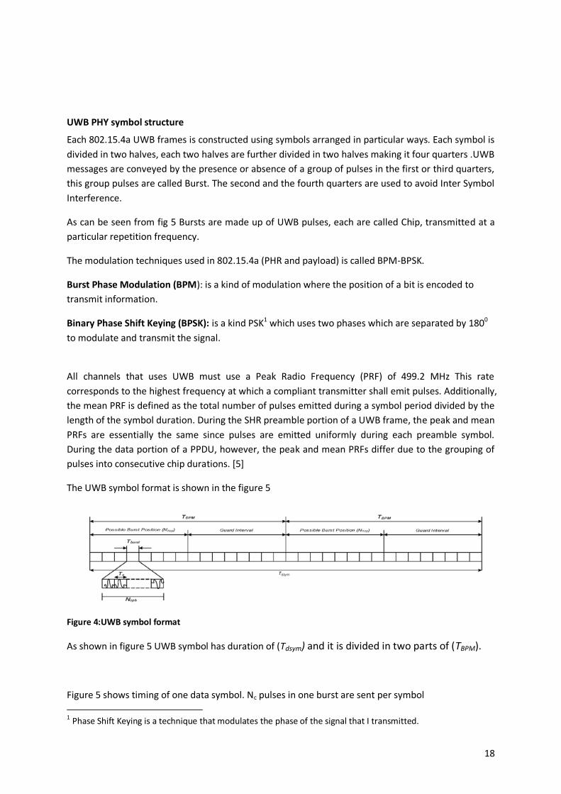
UWB PHY symbol structure

Each 802.15.4a UWB frames is constructed using symbols arranged in particular ways. Each symbol is

divided in two halves, each two halves are further divided in two halves making it four quarters .UWB

messages are conveyed by the presence or absence of a group of pulses in the first or third quarters,

this group pulses are called Burst. The second and the fourth quarters are used to avoid Inter Symbol

Interference.

As can be seen from fig 5 Bursts are made up of UWB pulses, each are called Chip, transmitted at a

particular repetition frequency.

The modulation techniques used in 802.15.4a (PHR and payload) is called BPM-BPSK.

Burst Phase Modulation (BPM): is a kind of modulation where the position of a bit is encoded to

transmit information.

Binary Phase Shift Keying (BPSK): is a kind PSK1 which uses two phases which are separated by 1800

to modulate and transmit the signal.

All channels that uses UWB must use a Peak Radio Frequency (PRF) of 499.2 MHz This rate

corresponds to the highest frequency at which a compliant transmitter shall emit pulses. Additionally,

the mean PRF is defined as the total number of pulses emitted during a symbol period divided by the

length of the symbol duration. During the SHR preamble portion of a UWB frame, the peak and mean

PRFs are essentially the same since pulses are emitted uniformly during each preamble symbol.

During the data portion of a PPDU, however, the peak and mean PRFs differ due to the grouping of

pulses into consecutive chip durations. [5]

The UWB symbol format is shown in the figure 5

Figure 4:UWB symbol format

As shown in figure 5 UWB symbol has duration of (Tdsym) and it is divided in two parts of (TBPM).

Figure 5 shows timing of one data symbol. Nc pulses in one burst are sent per symbol

1 Phase Shift Keying is a technique that modulates the phase of the signal that I transmitted.

19

Random spreading sequence

Nc can be 512, 128, 32, 16, 8, 4, 2, 1

Burst hopping (Nhop = 2, 8, 32)

Guard Interval

2.1.3 Architecture of WSN

A single sensor cannot fulfil the task of the WSN by itself, it must a collaborate with other sensor

nodes in wireless medium.

This sub chapter discusses the architecture of WSN starting from single node architecture to

communication architecture

2.1.3.1 Sensor Node Architecture

A basic component of a WSN node is shown in Fig 5.These components should operate in such a way

that they minimize the power consumption of the node. This is because power or energy is a very

scarce resource in WSN.

Memory

Communication

DeviceController

Sensor

Device

Power Supply

Figure 5:WSN node Architecture[17]

Each part in Fig 5 is described as follows:

Controller: is to process relevant data and capable of executing some kind of code. E.g. MSP430,

STM32c cortex M3, ATMEL AVR.

Memory: is for storing intermediate data and programs

Sensor Device: is the actual interface to the environment, this part should be capable of sensing the

environment. E.g. thermometer, pressure sensors, light sensors.

Power supply: is power supplier to the system, this can be batteries or main power grid.

20

Communication Device: is used for sending and receiving data. To be able to interact to the actual

environment a node should have both transmitter and receiver.

In our implementation:

The Tag has: Texas instrument’s MSP430f5438A microcontroller with 16KB of RAM and 256KB of

Flash memory, battery supplied power

The Anchors and the coordinator have: ARM’s STM32 cortex M3 microprocessor with 64KB and

256KB of Flash memory, power is supplied from the grid.

2.1.2.2 Communication Architecture

As in any kind of communication network devices WSN nodes must have suitable communication

architectures. Fig 6 shows typical communication architecture for wireless sensor network. But

different architectures are designed for deferent applications.

Application layer

Transport layer

Network layer

MAC layer

PHY layer

Figure 6: Sensor network architecture

The protocols that are used on different parts of this wireless sensor network are different from the

normal protocol that is used in wired and wireless networks. They need to support various

specification, requirements and constraints such as memory, battery, fault tolerance system and

robustness. [9].The design of wireless sensor network protocol must take consideration of

Reliability: it is the ability to sustain the working functionality of the sensors. Sensors may

stop working due to energy lack or physical damage…

Scalability: the protocol must be able to handle large number of nodes in WSN

Energy Consumption

Hardware Constraint.

21

Physical Layer (PHY)

The task of the physical layer is to modulate and demodulate the digital data; this function is done by

digital transceivers. In sensor network architecture the challenge is to design a transceiver that is low

cost and low battery consumption. [10]

The design of the PHY layer for wireless sensor network must take this into an account

Low Power Consumption

Low duty cycles

Lower data rates

Low implementation complexity

In our implementation we have used an IEEE 802.15.4a PHY described in 2.1.2.3, because it

low complex, low cost and has precise ranging measurement.

Medium Access Layer (MAC)

The MAC layer controls access to the shared medium and checks weather there is a collision or not.

The MAC should be able to reduce the energy wastage presented in WSN node. The potential energy

wastage could be: [7]

Collision: Hearing collided packets

Overhearing: receiving packets destined for other packets.

Idle listening: listening to idle channel for receiving possible traffic.

Over emitting: is transmitting of the message when the destination node is not ready.

A good MAC layer protocol should avoid these energy wastages.

A well-defined MAC layer protocol should also be scalable i.e. any increase in network size and

density should be effectively handled, adaptable to any changes. Changes attributed to network size,

node density should be handled rapidly and effectively. [7]

Available MAC protocols for WSN

According to [2] the MAC layers for sensor networks can be classifies as Contention based and Schedule based.

Contention Based

Here the access to the medium is distributed, meaning there is no central which can control the

medium. Examples include the following.

22

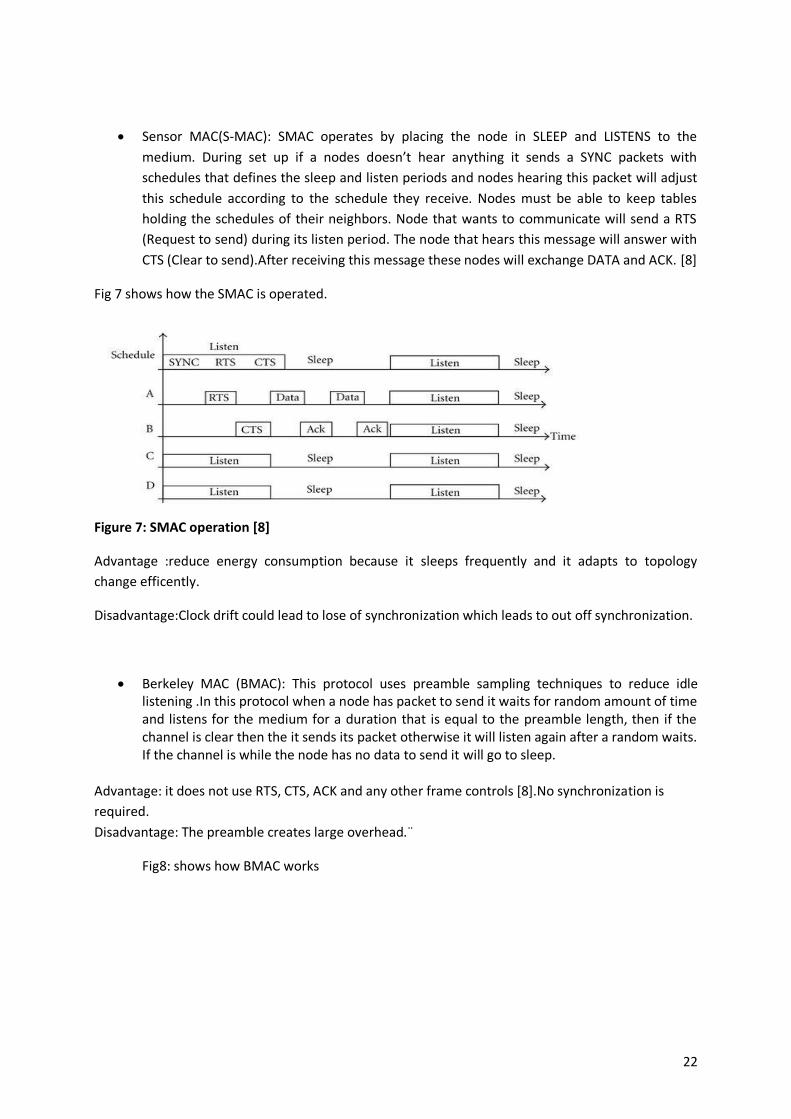
Sensor MAC(S-MAC): SMAC operates by placing the node in SLEEP and LISTENS to the

medium. During set up if a nodes doesn’t hear anything it sends a SYNC packets with

schedules that defines the sleep and listen periods and nodes hearing this packet will adjust

this schedule according to the schedule they receive. Nodes must be able to keep tables

holding the schedules of their neighbors. Node that wants to communicate will send a RTS

(Request to send) during its listen period. The node that hears this message will answer with

CTS (Clear to send).After receiving this message these nodes will exchange DATA and ACK. [8]

Fig 7 shows how the SMAC is operated.

Figure 7: SMAC operation [8]

Advantage :reduce energy consumption because it sleeps frequently and it adapts to topology

change efficently.

Disadvantage:Clock drift could lead to lose of synchronization which leads to out off synchronization.

Berkeley MAC (BMAC): This protocol uses preamble sampling techniques to reduce idle listening .In this protocol when a node has packet to send it waits for random amount of time and listens for the medium for a duration that is equal to the preamble length, then if the channel is clear then the it sends its packet otherwise it will listen again after a random waits. If the channel is while the node has no data to send it will go to sleep.

Advantage: it does not use RTS, CTS, ACK and any other frame controls [8].No synchronization is

required.

Disadvantage: The preamble creates large overhead.¨

Fig8: shows how BMAC works

23

Figure 8: BMAC operation [8]

Dynamic MAC (DMAC):is an improved form of slotted ALOHA ,in which slots are assigned to

the nodes based on the position of the node in the data gathering tree as shown in Fig 9.

Figure 9: DMAC operations [11]

In DMAC if a node is in Rx mode then all its child’s must be either in Tx mode or in contention for the

medium mode. To obtain low latency it can be assigned subsequent slots to the modes that are

successive in data transmission. [11]

Advantage:DMAC has better sleep/listen period latency.

Disadvantage:DMAC doesnot employe any form collision avoidance scheme,if two or

more nodes tries to send packet at the same time then collision could occur.

Time-Out MAC(TMAC): is an improvement for SMAC by assigning dynamic duty cycles, which

very suitable for delay sensitive applications [12].In TMAC the listen period ends when there

is no event for has happened for threshold τ. Since there are nodes at different parts of the

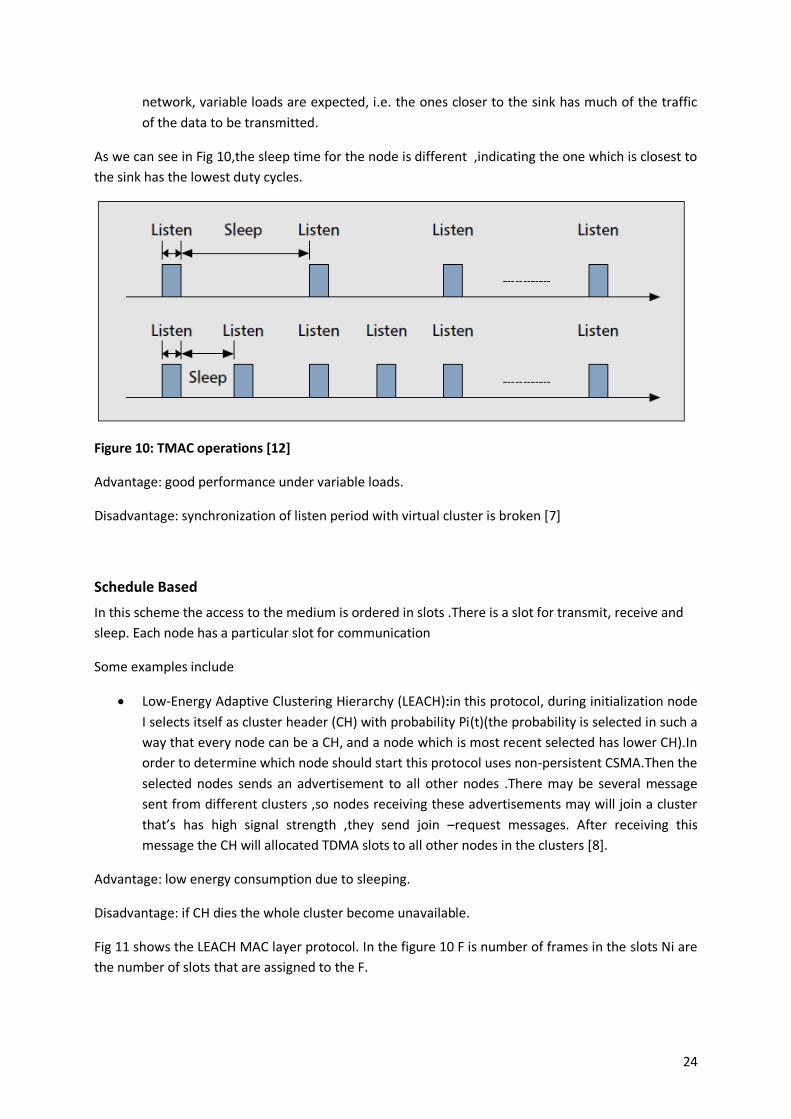
24

network, variable loads are expected, i.e. the ones closer to the sink has much of the traffic

of the data to be transmitted.

As we can see in Fig 10,the sleep time for the node is different ,indicating the one which is closest to

the sink has the lowest duty cycles.

Figure 10: TMAC operations [12]

Advantage: good performance under variable loads.

Disadvantage: synchronization of listen period with virtual cluster is broken [7]

Schedule Based

In this scheme the access to the medium is ordered in slots .There is a slot for transmit, receive and

sleep. Each node has a particular slot for communication

Some examples include

Low-Energy Adaptive Clustering Hierarchy (LEACH):in this protocol, during initialization node

I selects itself as cluster header (CH) with probability Pi(t)(the probability is selected in such a

way that every node can be a CH, and a node which is most recent selected has lower CH).In

order to determine which node should start this protocol uses non-persistent CSMA.Then the

selected nodes sends an advertisement to all other nodes .There may be several message

sent from different clusters ,so nodes receiving these advertisements may will join a cluster

that’s has high signal strength ,they send join –request messages. After receiving this

message the CH will allocated TDMA slots to all other nodes in the clusters [8].

Advantage: low energy consumption due to sleeping.

Disadvantage: if CH dies the whole cluster become unavailable.

Fig 11 shows the LEACH MAC layer protocol. In the figure 10 F is number of frames in the slots Ni are

the number of slots that are assigned to the F.

25

Figure 11: LEACH operation. [8]

Power-Efficient and Delay-Aware Medium Access Protocol (PEDAMACS): This protocol

assumes there is an access point (AP), which can reach the other nodes with one hop.

However, the sensor can reach with more than hop. The power levels can be classified as the

maximum, minimum and medium. This protocol has three phases:

Topology Discovering: here the access point (AP) broadcast a SYNC packets to all

nodes .After the SYNC packets the AP sends another packet to all nodes to tell them that

they belong to this cluster which the AP administer, this packet is retransmitted through

the entire network, and if nodes receive more than one, then the node chooses the

cluster based on the received signal strength. During this period the protocol employs

RTS and CTS similar to 802.11.

Topology Collection: in this phase the nodes sends the topology to the AP.

Scheduling Phase: here the AP sends the scheduling algorithm with which the node in

the cluster operates i.e. when they are going to receive and transmit the rest of time

they sleep.

Advantage: it is quite suitable for event driven sensing.

Disadvantage: overhead associated with RTS, CTS.

In Fig 12 the sent packets by the nodes are denoted by solid arrow and that of node are denoted by

AP

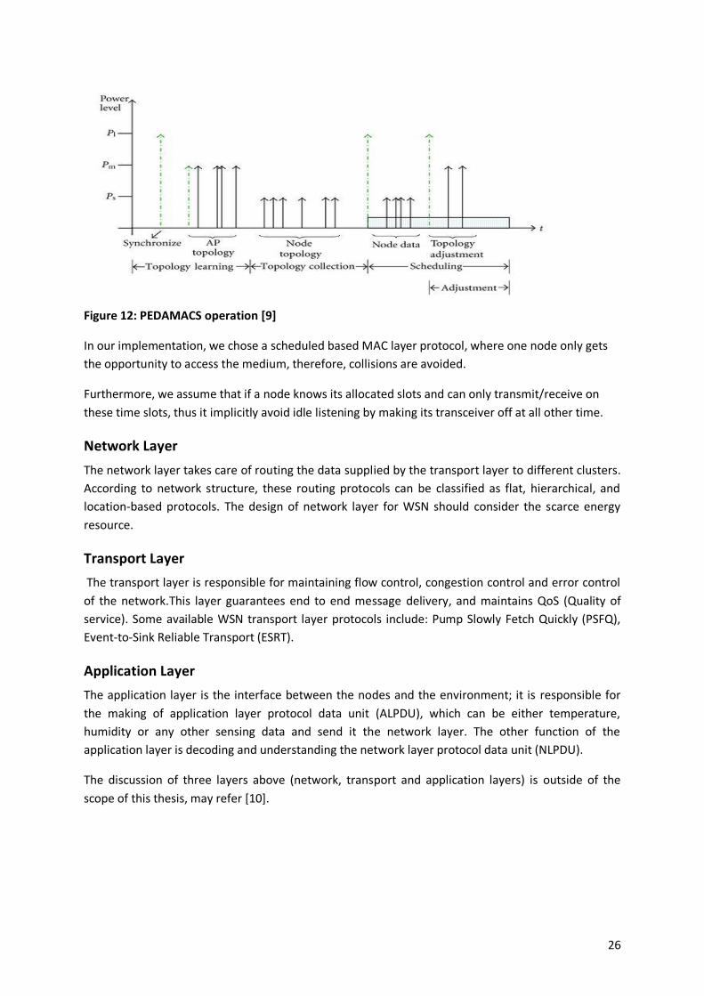
26

Figure 12: PEDAMACS operation [9]

In our implementation, we chose a scheduled based MAC layer protocol, where one node only gets

the opportunity to access the medium, therefore, collisions are avoided.

Furthermore, we assume that if a node knows its allocated slots and can only transmit/receive on

these time slots, thus it implicitly avoid idle listening by making its transceiver off at all other time.

Network Layer

The network layer takes care of routing the data supplied by the transport layer to different clusters.

According to network structure, these routing protocols can be classified as flat, hierarchical, and

location-based protocols. The design of network layer for WSN should consider the scarce energy

resource.

Transport Layer

The transport layer is responsible for maintaining flow control, congestion control and error control

of the network.This layer guarantees end to end message delivery, and maintains QoS (Quality of

service). Some available WSN transport layer protocols include: Pump Slowly Fetch Quickly (PSFQ),

Event-to-Sink Reliable Transport (ESRT).

Application Layer

The application layer is the interface between the nodes and the environment; it is responsible for

the making of application layer protocol data unit (ALPDU), which can be either temperature,

humidity or any other sensing data and send it the network layer. The other function of the

application layer is decoding and understanding the network layer protocol data unit (NLPDU).

The discussion of three layers above (network, transport and application layers) is outside of the

scope of this thesis, may refer [10].

27

2.2 Indoor Positioning Systems

An indoor positioning system determines the location of an object in indoor environment such as

warehouse, buildings etc., it is assumed that the position is done in real-time or near real-time by

tracking an object moving in in space. [13].

Bases on the physical signal that is used for positioning ,indoor positioning can be classified into

three types .The discussion are described in detail in the following subsections.

2.2.1 Infrared positioning systems

Here an infrared signal is used for signal transmission. The system contains infrared sensors which

are deployed in the building. Objects to be tracked emits infrared signal with a unique identifier in

every 10-20sec.The IR sensors collect this data and sent to the central server, which in turn calculates

the position either using TOA (Time of Arrivals) or Trilateration. The problem with IR system is it is

limited to Line of Sight (LOS).The accuracy is good but not the coverage area. [13]

2.2.2. Optical positioning system

Here an optical signal is used for signal transmission. A good example for this is CLIPS (Camera and

Laser based Indoor Positioning System).This system contains a laser device and a camera, the camera

device acts as a mobile device. The laser device is oriented towards to the ceiling, and laser beams

are installed on the ceiling. Then camera device tracks the laser beams. [12].This system has very

high accuracy, but maximum coverage area in 10-15m.

2.2.3 Radio frequency positioning system

Here a radio frequency (RF) is used for signal transmission. The most common types of RF system are

RFID (Radio Frequency Identification), Bluetooth, WLAN (Wireless Local Area Network) and UWB

positioning.

2.2.3.1 RFID

The system contains RFID readers and RFID transmitters .In this system receive signal strength

information (RSSI) is used by the RFID readers to determine the location of the RFID transmitter. The

coverage area of the system is in the range of meters which makes it worst choice.

2.2.3.2 Bluetooth

This system contains Bluetooth beacons which are installed in the building and a Bluetooth enabled

mobile device. In this system RSSI in the beacons can be used to track the mobile device .The system

has a coverage area of 50m but the accuracy of the system is 5-10m which is worst.

2.2.3.3 WLAN or WIFI positioning

This system uses fingerprinting where observation are compared to the previously mapped

observation or trilateration which is discussed in 2.3.2, techniques to get the position of the mobile

device. This system can offer us up to ±5cm accuracy which may not be enough for real time location

systems

28

2.2.3.4 Ultra wide band positioning system

In this system a short pulse of UWB IR is used.UWB has very high bandwidth and high resistance to

fading. This system has nodes which are deployed in a known location and a mobile node. A mobile

node will broadcast a UWB signal, which is received by the nodes at different time .Then this nodes

will transmit the received time to central coordinator which can calculate based on TOA or TDOA

techniques. This system could reach to ±10cm; together with it resistance to fading it will make it the

ideal choice for indoor positioning.

Fig 13 shows the indoor positioning techniques.

Figure 13: Indoor Positioning Techniques [18]

29

3. Ranging and Localization

This chapter discusses ranging and localization algorithms in general. Section 3.1 discusses what is

ranging, how we can achieve ranging and its types. Section 3.2 discusses what localization is and how

we can perform localization.

3.1Ranging

Ranging is a method of finding one location relative to another location or it will tell how far one

device is located from another device. Fig 14 shows ranging. In ranging the device that wants to

measure the distance only knows how far the other device is located.

Figure 14: Ranging

As can be seen from Fig 14, the inner star want to know the location of the outer star but ranging can

only tell us how far is it from the inner star ,but not the direction, so actually the outer star could be

located at any place in radius of the of the circle.

Two types of ranging are implemented in IEEE802.15.4a: private ranging and standard ranging. [5]

3.1.1Standard Ranging

According to [5] the IEEE802.15.4a standards uses 31 chip long preamble sequence .Figure 15 Shows

standard ranging between two devices .Device A initiates ranging by sending RReq packet to Device B

and activates a counter when the packet departs from A. Device B upon receiving it activates its

counter and responds with a RRep and a time stamp report back to A.When RRep reaches A device A

measure the time differences. The timestamp report contains information about start-to -stop time;

figure of merit, tracking offsets and total tracking interval. The crystal offset between the two devices

can be calculated from the received tracking offset and total tracking interval. Figure of merit

parameter tells device A the confidence of the measurement. [20]

30

Device ADevice B

RReq

RRep

Timestamp reprt

t1

t3

t4

t6

t5

t3

Figure 15:Standard Ranging

3.1.2Private Ranging

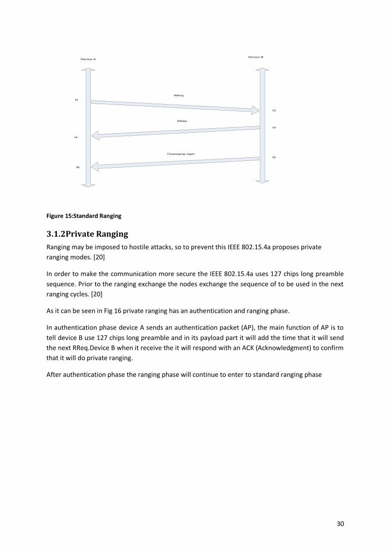
Ranging may be imposed to hostile attacks, so to prevent this IEEE 802.15.4a proposes private

ranging modes. [20]

In order to make the communication more secure the IEEE 802.15.4a uses 127 chips long preamble

sequence. Prior to the ranging exchange the nodes exchange the sequence of to be used in the next

ranging cycles. [20]

As it can be seen in Fig 16 private ranging has an authentication and ranging phase.

In authentication phase device A sends an authentication packet (AP), the main function of AP is to

tell device B use 127 chips long preamble and in its payload part it will add the time that it will send

the next RReq.Device B when it receive the it will respond with an ACK (Acknowledgment) to confirm

that it will do private ranging.

After authentication phase the ranging phase will continue to enter to standard ranging phase

31

Device ADevice B

RReq

RRep

Timestamp reprt

t1

t3

t4

t6

t5

t3

AP

Authentication

Figure 16: Private Ranging

Ranging does not tell us the exact position i.e. the coordinate axes that the mobile device is located;

it only tells the distance between the two nodes. The good thing with ranging is it does not need

explicit synchronization phase, because they can measure the timestamp when they receive and

send packets and calculate the clock offset of each other.

3.2Localization

Localization is a technique used to determine accurate position i.e. the coordinate axes, of a mobile

node by using either the difference in time of the arrival of time at a known location or by using angle

between the nodes. Sine we have used the arrival of time concept for our implementation; only the

difference in time of arrival is discussed here, interested reader on angle of arrival between the nodes

can refer [17].

3.2.1 Time of arrivals (TOA)

Time of arrivals system works by determining total time required for the radio signal to propagate

from a transmitter to a receiver. If this time is determined accurately then the distance between the

transmitter and the receiver can be determined since the speed of radio propagation in air is known.

TOA arrival assumes the mobile device and the nodes at fixed position are synchronized in time

The main idea behind TOA is shown in Fig 17. The mobile device (D) in the Fig 17, broadcast a

message which contains the transmit time as a payload to all nodes (A, B, C) .Since they all are

synchronized to the same time base ,each nodes(A,B,C) can calculate the time of flight by

subtracting the transmit time from the received time. After that they can calculate the distance

between themselves and node D denoted (Ra, Rb and Rc) by multiplying the time of flight by speed

of light.

After that they can pass this information to central controller which can calculate based on eq (3.1)

and (3.2).

32

A

B

C

DRa

Rb

Rc

Figure 17: TOA Positioning

Ra=

Rb= ---------------- (3.1)

Rc=

When those three points A, B, C are not collinear, that is, the following matrix:

--------------------------------- (3.2)

is nonsingular, then, from solving (4.1), we obtain the estimation position of the unknown sensor for

D(x, y):

This system needs 3 fixed location nodes for 2D measurements, and 4 fixed nodes for 3D measurements

The drawback of this system is, it needs all system to be synchronized to the same time base, and

this can be achieved between fixed positioned nodes but it may be difficult to achieve between the

mobile nodes and fixed nodes.

3.2.2 Time Difference of Arrival (TDOA)

In TDOA system three or more reference nodes are positioned at known locations and must also be

synchronized among each other. The mobile device which is going to be tracked must operate

around these reference nodes.

33

In TDOA the mobile nodes initiates a range request by sending single message to all

neighboring .Because radio waves travels at a constant speed, depending on the relative position of

the reference node to the mobile node the message will arrive at different time, this time is noted by

the receiver and pass it to the central coordinator who can calculate the distance using

multilateration (eq3.3). [4]

The calculation of the distance is as follows:

Let’s assume the tag is located at point (X,Y,Z)and TL, TQ, TC, TR, are arrival times at the fixed

points of at the left, right, quadrant and coordinator and given by eq 3.3

eq………….(3.3)

The difference in time between the coordinator and the other ia calculated as follows

Where (XL,YL,ZL) is the location of the left receiver site, and soon, and is the speed light. Each

equation defines a separate hyperboloid. The intersection of the all hyperbolas defines the exact

position of the mobile node as shown in fig 18.

34

Figure 18:TDOA Positioning

Table 3 shows the typical error in loss of synchronization in TOA and TDOA case.

Error (µs) 2ppm (ns) 20ppm (ns) 40ppm(ns)

1 0.0005 0.005 0.01

10 0.005 0.05 0.1

100 0.05 0.5 1

Table 3: Typical errors in synchronizations

As it shows in the clock difference in 0.0005 ns would result in 1µs error in time measurement in

2ppm crystal oscillator.

For correct computation of position we need a clock difference of 0.1 ns at most for our device in

order to get the position with in ±25cm.

We select TDOA for our implementation because we want to calculate the locations on the position

servere and pass it to map to show it in real time.

35

4 Design and Implementation

This chapter discusses about the implementation of our system, it further discusses what kind of

hardware we used, the packet format that we exchanged, and the design procedures of the medium

access control.

The goal of the implementation is to design a positioning system that can track an asset or a person

to the accuracy ±25cm and gives a battery life up to 3 years.

This chapter has the following outline

4.1. Discusses the system overview and the hardware components of our system.

4.2. Discusses the protocol architecture of each kind of devices in our system.

4.3. Discusses the implementation and results of the peer -to-peer ranging system

4.4 Discusses the design of the medium access control and how scheduling can be done for the

implementation of the whole system.

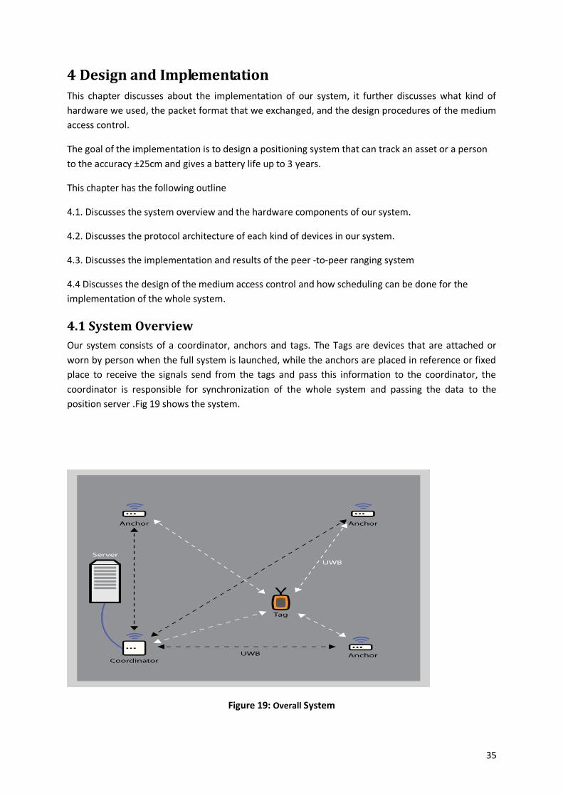
4.1 System Overview

Our system consists of a coordinator, anchors and tags. The Tags are devices that are attached or

worn by person when the full system is launched, while the anchors are placed in reference or fixed

place to receive the signals send from the tags and pass this information to the coordinator, the

coordinator is responsible for synchronization of the whole system and passing the data to the

position server .Fig 19 shows the system.

Figure 19: Overall System

36

4.1.1Hardware Components

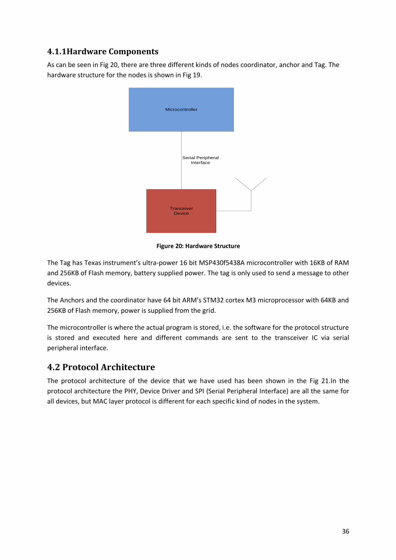
As can be seen in Fig 20, there are three different kinds of nodes coordinator, anchor and Tag. The

hardware structure for the nodes is shown in Fig 19.

Microcontroller

Tranceiver

Device

Serial Peripheral

Interface

Figure 20: Hardware Structure

The Tag has Texas instrument’s ultra-power 16 bit MSP430f5438A microcontroller with 16KB of RAM

and 256KB of Flash memory, battery supplied power. The tag is only used to send a message to other

devices.

The Anchors and the coordinator have 64 bit ARM’s STM32 cortex M3 microprocessor with 64KB and

256KB of Flash memory, power is supplied from the grid.

The microcontroller is where the actual program is stored, i.e. the software for the protocol structure

is stored and executed here and different commands are sent to the transceiver IC via serial

peripheral interface.

4.2 Protocol Architecture

The protocol architecture of the device that we have used has been shown in the Fig 21.In the

protocol architecture the PHY, Device Driver and SPI (Serial Peripheral Interface) are all the same for

all devices, but MAC layer protocol is different for each specific kind of nodes in the system.

37

Figure 21: Protocol Architecture

4.2.1 SPI interface

The SPI interface that we use is very simple open SPI communication, close SPI communications and

multiple read /writes operations between the micro-controller and the transceiver IC.

4.2.2 Device Driver

This is the driver software that we get from the transceiver manufacturer for the transceiver IC which

works only for the computer, but we optimized it by changing the data types and some data

structures so that the program can work in microcontroller.

4.2.3 PHY Layer

This provides the API according to 802.15.4a standard for UWB PHY.The standard defines this API’s

as a primitive operation.Prinitives originated from the MAC layer is called request primitives, and

they are responded with confirm primitives from the physical layer. The third even is called

indication-primitive which are generated from the PHY and sent to the MAC layer. When something

happen in the PHY like packet reception. This message exchange is discussed in 4.3

4.2.4 MAC Layer

This layer provide the API for 802.15.4a and responsible for controlling the shared access of the

medium .Since the system that is intended to be implemented is requires low battery utilization then

we choose to use scheduled time slots which is discussed.4.4.3.

4.3 Peer-to-Peer (P2P) Ranging Implementation

This subchapter discusses the peer-to-peer implementation, packet format and overall

communication architectures

4.3.1 P2P Message Exchange

In our P2P implementation we make communication only between the tag and one of the anchors.

The overall detail of the communication architecture is discussed in the following paragraph.

The IEEE 802.15.4a standard [5] states three kinds of message that the MAC layer issues to the PHY

layer. These are request, response and indirections.

38

In our implementation, the mechanism that is used is to make these primitives as identified

enumerated. The MAC layer above writes these to the PHY layer which are picked up by the physical

layer. The PHY layer has its own data structure that can pick the primitive from the MAC and also to

send the response to the MAC if it is a request primitive.

The MAC writes the primitive to a fixed primitive data structure that is picked up by the PHY. For

synchronization a primitive ID of EMPTY is also declared to indicate no primitive is available.

When the PHY reads a primitive it will set the ID to EMPTY so the MAC knows it can write another if

required.

The input primitives are written to the pip (phyinputprimitive_t) within the phydatablock_t this is

the area to write the PHY (request/response) primitive input messages.

In a similar way the PHY will write primitive response messages to an output structure which can be

picked up by the MAC and the MAC reads the data structure to pick up the response.

A primitive ID of EMPTY is declared to indicate no primitive response is available at this time. After

seeing a response the MAC should set the primitive ID to EMPTY to allow the PHY to give additional

responses/indication messages to the MAC.

The input primitives are picked up from the pop (phyoutputprimitive_t) within the phydatablock_t

this is the area to pick up PHY (confirm/indication) primitive output messages.

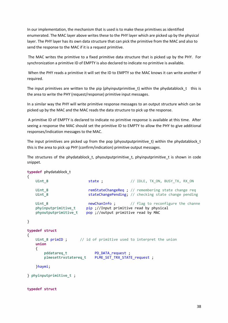
The structures of the phydatablock_t, phyoutputprimitive_t, phyinputprimitive_t is shown in code snippet.

typedef phydatablock_t { Uint_8 state ; // IDLE, TX_ON, BUSY_TX, RX_ON Uint_8 remStateChangeReq ; // remembering state change req Uint_8 stateChangePending; // checking state change pending

Uint_8 newChanInfo ; // flag to reconfigure the channe phyinputprimitive_t pip ;//Input primitive read by physical

phyoutputprimitive_t pop ;//output primitive read by MAC } typedef struct { Uint_8 primID ; // id of primitive used to interpret the union union { pddatareq_t PD_DATA_request ; plmesettrxstatereq_t PLME_SET_TRX_STATE_request ; }haymi; } phyinputprimitive_t ; typedef struct

39

{ Uint_8 primID ; // id of primitive used to interpret the union union { pddataconf_t PD_DATA_confirm ; pddataind_t PD_DATA_indication ; plmesettrxstateconf_t PLME_SET_TRX_STATE_confirm ; }baby; } phyoutputprimitive_t ;

As can be seen from the code snippet the phyinputprimitive_t contain structures of the standard

PD_DATA_Req and PLME_SET_TRX_STATE_Req ,in which both are input to the PHY layer and output

from the MAC.

The phyinputprimitive_t data structure contains PD_DATA_Conf ,PD_DATA_INDICATION and

PLME_SET_TRX_STATE_Conf which are written by the PHY layer and picked up by the MAC layer.

Table 3 shows the Message Exchange between the PHY and MAC sub layers.

MESSAGES MAC TO PHY MESSAGES PHY TO MAC

=================== ===================

1) Immediate Functions

PLME-GET.request

PLME-GET.confirm

PLME-SET.request

PLME-SET.confirm

2) Delayed Transactions

PD-DATA.request

PD-DATA.confirm

PD-DATA.indication

PD-DATA.timeout

PLME-SET-TRX-STATE.request

PLME-SET-TRX-STATE.confirm

Table 4: Message Exchange between PHY and MAC

As can be seen in table 3 the messages can be classified as immediate or delayed transactions, where

the immediate ones are the ones that are responded by PHY immediately but the delayed one like

(PD_DATA_Req which is indicate there is data to be sent may be delayed because PHY must wait

until the data is sent to respond to the MAC).The sequence diagram in Fig 22 describes the message

exchange between two peer to peer devices

40

Sender Receiver

PLME_SET_TRX_STATE_Req

State:TX

MAC MACPHYPHY

PLME_SET_TRX_STATE_Confi

State:sucess

PD_DATA_Req

Ranging On


State:RX with ranging


State:sucess

DATA_With Ranging Req

PD_DATA_Confirm

Status:OK

PD_DATA_Indication


State:TX


State:sucess


State:RX with ranging


State:sucess

PD_DATA_Req

Ranging On

DATA_With Ranging Req

PD_DATA_Indication

Figure 22: Sequence flow for two peer to peer message exchanges

The receiver MAC issues PLME_SET_TRX_STATE_Req with RX_ON with rangingto the PHY, then the

PHY responds with orders PLME_SET_TRX_STATE_Confirm with state RX with ranging on if it

successful otherwise it will respond with Fail so the MAC should issue the PLME_SET_TRX_STATE_req

again. If it is successful then the receiver will be on the receive mode waiting for the data to be

received.

The Sender MAC issues PLME_SET_TRX_STATE_Req with TX_ON the PHY, then the PHY responds

with orders PLME_SET_TRX_STATE_Confirm with state TX on successful otherwise it will respond

with Fail so the MAC should issue the PLME_SET_TRX_STATE_req again. If it is successful then the

sender MAC prepares data and issue PD_DATA _Req to the PHY ,then the PHY accepts this DATA

request and try to send the data if it is successful then it issues PD_DATA_Confirm with OK ,if not it

will issue PD_DATA_Confirm with FAIL so the MAC can resend it again.

41

The receiver PHY which is on receiving state after getting the Data it will issue PD_DATA_Indication

so that the MAC can process.

The response message is from the receiver to the sender is follows the same procedure.

4.3.2 Message Exchanged and Their Formats

The IEEE 802.15.4 MAC frame format is shown in the fig. 23

Frame Control

2bytes

Sequence Number

1bytes

PANID

2bytes

Destination Address

8bytes

Source Address

8bytes

Payload

0-127bytes

FCS

2bytes

Ranging Frame

First 32 Bytes of the Payload

Figure 23: MAC Frame

The format contains

Frame Control: describes what kind of frame types we used e.g. Beacon, Data,

Acknowledgment, MAC command.

Sequence Number: denotes the sequence of the bytes sent

PANID: it is the ID of the Personal Area Network (PAN), which we haven’t used this because

we don’t have a cluster.

Destination Address: the address of the destination node.

Source Address: the address of the source address.

Payload: the data part we take some bytes to make our ranging frame.

FCS: frame check sequence added by the transceiver IC for error correction.

In P2P implementation we have designed and use four kinds of messages which are discussed as

follows

Poll Message: the poll message for P2P implementation is sent by the tag to initiate ranging

communication with the anchor. For a POLL message the ranging message portion of the frame only

contains a single octet designated by 0x01, this is denoted by Function Code part of the frame

Response Message: the response message for P2P application is sent by the anchor in response to

the POLL message received from the tag. For the response message we use a single octet with value

0x02 to differentiate it from others.

42

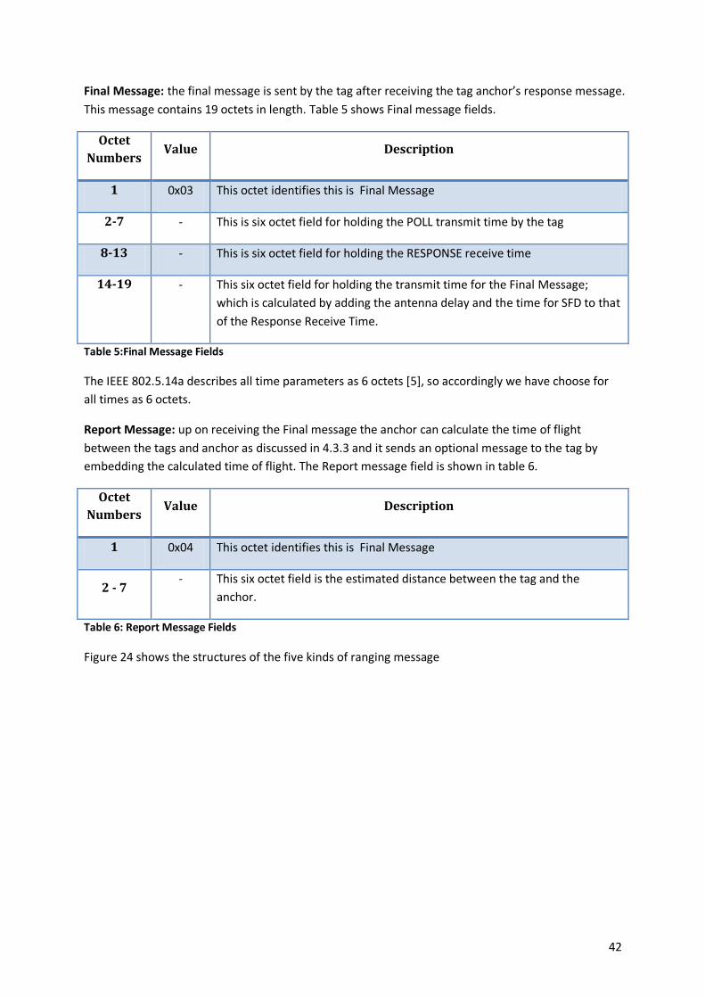
Final Message: the final message is sent by the tag after receiving the tag anchor’s response message.

This message contains 19 octets in length. Table 5 shows Final message fields.

Octet

Numbers Value Description

1 0x03 This octet identifies this is Final Message

2-7 - This is six octet field for holding the POLL transmit time by the tag

8-13 - This is six octet field for holding the RESPONSE receive time

14-19 - This six octet field for holding the transmit time for the Final Message;

which is calculated by adding the antenna delay and the time for SFD to that

of the Response Receive Time.

Table 5:Final Message Fields

The IEEE 802.5.14a describes all time parameters as 6 octets [5], so accordingly we have choose for

all times as 6 octets.

Report Message: up on receiving the Final message the anchor can calculate the time of flight

between the tags and anchor as discussed in 4.3.3 and it sends an optional message to the tag by

embedding the calculated time of flight. The Report message field is shown in table 6.

Octet

Numbers Value Description

1 0x04 This octet identifies this is Final Message

2 - 7 - This six octet field is the estimated distance between the tag and the

anchor.

Table 6: Report Message Fields

Figure 24 shows the structures of the five kinds of ranging message

42

Poll Message Response Message

0x01 -

Functional Code

1byte

Optional Data Bytes

0-31 Bytes

0x02 -

Functional Code

1byte

Optional Data Bytes

0-31 Bytes

Final Message

0x03 -

Functional Code

1byte

POLLTX Time

6 bytes

Optional Data Bytes

0-13 Bytes

-

RESPONS TX Time

6 bytes

- -

Predicted Final TX Time

6 bytes

Report Message

0x04 -

Functional Code

1byte

Calculated Time of

Flight

6bytes

Optional Data Bytes

0-25 Bytes

-

Figure 24: Encoding format of the ranging Message

4.3.3 Discussion and Results of P2P implementation

In our P2P implementation the MAC layer provides a simple ranging application i.e. it is where the

ranging calculation is performed.

Fig 25 shows the arrangement and the operation of the P2P implementation.

In the implementation the anchor turns on its receiver and waits indefinitely for a poll message from

the tag. The tag sends a poll and wait for a response from the anchor, after which sends the final

message .If the anchor response is not received in time, the tag times our and send the poll message

again. After receiving the poll the anchor sends the response message and waits for the final

message, after receiving the final message it will calculate the time of flight as in eq 4.1 and send

report to the tag or to the position server .Fig 24 shows the arrangement and the operation of the

P2P implementation.

Tag Anchor

RESPONSE

FINAL

REPORT

Calculate

Range

POLL

Listen To

POLL

Figure 25:P2P Ranging Implementation

43

Time of Flight calculation is calculated as shows below:

POLL-RESPONSE round trip time is given by:

(Response RX Time-Poll TX Time)-(Response TX Time-POLL RX Time)

RESPONSE-FINAL round trip time is given by:

(FINAL RX Time-RESPONSE TX Time)- (FINAL TX Time-RESPONSE RX Time)

TOF is given by:

…………. (4.1)

The following tables show the result obtained in P2P implementation in LOS and NLOS condition.

LOS measurement:

Number of

Transmitted

Packets

Number of Received

Packets TOF calculation

Instant Measured

Distance

Mean of Calculated

Distance (Last 8)

1 2 129.222 ns 38.728m 38.728m

3 4 129.376ns 38.812m 38.77m

5 6 129.187ns 38.756m 38.763m

.

.

.

.

.

.

.

.

.

.

.

.

.

.

.

15 16 129.276ns 38.782m 38.769m

17 18 129.199ns 38.759m 38.763m

.

.

.

.

.

.

.

.

.

.

.

.

.

.

.

55 56 130.444ns 39.133m 38.784m

57 58 129.014ns 38.704m 38.781m

Actual Distance between the tag and the anchor is 38.96m Table 7:P2P LOS measurement

As it is shown in table 7 the measurements are done in anchor side the deviation of the

measurement is well below what we have expected .The maximum deviation is from the normal

measured distance is 38.704m which is 25.6cm.

NLOS measurements:

Here the measurement is done in an environment where two brick walls are existed between the tag

and the anchor. Table 8 shows the results of the measurement.

44

Number of

Transmitted

Packets

Number of Received

Packets TOF calculation

Instant Measured

Distance

Mean of Calculated

Distance (Last 8)

1 2 36.214ns 10.853m 10.853m

3 4 37.314ns 11.194m 11.023m

5 6 35.996ns 10.798m 10.948m

.

.

.

.

.

.

.

.

.

.

.

.

.

.

.

24 25 38.443ns 11.532m 11.094m

25 26 38.049ns 11.414m 11.158m

.

.

.

.

.

.

.

.

.

.

.

.

.

.

.

105 106 34.444ns 10.333m 11.073m

107 108 39.014ns 11.042m 11.006m

Actual Distance between the tag and the anchor is 10.39m Table 8:P2P NLOS Measurements

As it is shown in table 8 the measurements are done in anchor side the maximum deviation is from

the normal measured distance is 38.443m which is 1.145m.

As can be seen from the two measurement result, we can conclude that if we have a good LOS we

can achieve even better measurement that we expected. But the NLOS measurement indicate that

there will be some delay when the signals cross bricks between the tag and anchor ,so this leads to

an accuracy degradation in the measurement.

4.4 Implementation of Localization

Here we extend our implementation as shown in Fig 18.Fig 19 shows three kinds of devices ;tag,

anchors and coordinator. This subsection discusses the message types, the state of operation of each

types of device, the medium access design and the results can be discussed.

4.4.1 Message Exchanged for the localization

Poll Message: The poll message is sent by either the tag or the anchor in order to tell the coordinator

they are joining the network, each poll message is associated with time out i.e. if response message

is not received before the time out expires, they will send the poll message. The poll message may

piggyback data or not. The Poll message is the same as that of P2P implementations.

Response Message: are sent in response to the poll message by the coordinator. It is identified by

functional code 0x02.This message is the same as that of the P2P implementations.

Final Message: this is sent by either tag or anchor if the poll-response message is successful; this

message also has time out associated with it, if report (response by the coordinator) doesn’t reach in

time then, the communication is restarted by sending the poll message again. This message is

identified 0x03.The message fields are shown in Fig 25.

45

Report Message: this message is responded by the coordinator to the sender of the final message.

This message contains six time-stamps i.e. Poll Receive Time, Response Sent Time, Final Receive Time,

Sync time(offset),slot Numbers. It is denoted by 0x04.The Report message fields is shown in Fig 25.

Syn _time: describes the relative time drift between the sender of final message or coordinator.

Slot Number: The slot number which is used for synchronization purpose which described in section

4.4.3

TDOA message: this message tells the receivers that the sender is only sending the message for

TDOA calculations, this message can be sent either by tag or anchor. First, tag simply broadcast this

message to all nodes .The tag/anchor portion part of this message indicates weather it’s from the tag

or anchor. The Anchor transmits this message to the coordinator by adding the time of the received

time of the TDOA message from the tag to the coordinator. Then the coordinator sends this time

stamps to the position server. Section 4.4.3 discusses this in detail. The TDOA message fields are

shown in Fig 26.

0x03 -

Functional Code

1byte

Optional Data Bytes

0-31 Bytes

0x05 -

Functional Code

1byte

Anchor/Tag

1 bytes

TDOA Timestamps

6 bytes

-

Final Message TDOA message

0x04 -

Functional Code

1byte

POLL RX Time

6 bytesOptional Data Bytes

0-1 Bytes

-

RESPONSE TX Time

6 bytes

- -

Final RX Time

6 bytes

Syn_Time(offset)

6 bytes

-

Slot

Number

6 bytes

-

Report Message

Figure 26: Encoding format of localization

4.4.2 State transition

This discusses the state transition of the tag, the anchor and the coordinator. This section discusses

the state of the tag, anchor and coordinator.

4.4.2.1 The Tag State Transitions:

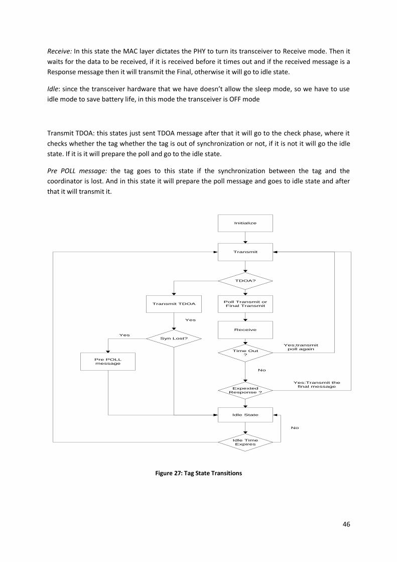
Fig 27 shows the state transition of the tag: each state is described as follows.

Initialize: In this state the device or the node is powered on ,and every architecture e.g. The

MAC,PHY,Device Driver and the SPI communication are checked whether they are working or not.

Transmit: In this state the MAC layer dictates the PHY to turn its transceiver to Transmit mode. After

the enters the transmit mode then it will check that the message to be sent is the

TDOA/(POLL/FINAL), if it is TDOA then it will go to TDOA Transmit ,else it will go to POLL/FINAL

transmit.

Poll/Final Transmit: here it transmits either poll or final and checks the associated time-out. If it is

time out at any phase it will transmit the poll again.

46

Receive: In this state the MAC layer dictates the PHY to turn its transceiver to Receive mode. Then it

waits for the data to be received, if it is received before it times out and if the received message is a

Response message then it will transmit the Final, otherwise it will go to idle state.

Idle: since the transceiver hardware that we have doesn’t allow the sleep mode, so we have to use

idle mode to save battery life, in this mode the transceiver is OFF mode

Transmit TDOA: this states just sent TDOA message after that it will go to the check phase, where it

checks whether the tag whether the tag is out of synchronization or not, if it is not it will go the idle

state. If it is it will prepare the poll and go to the idle state.

Pre POLL message: the tag goes to this state if the synchronization between the tag and the

coordinator is lost. And in this state it will prepare the poll message and goes to idle state and after

that it will transmit it.

Initialize

Transmit

Poll Transmit or

Final Transmit

No

Expexted

Response ?

Yes:Transmit the

final message

Idle State

Idle Time

Expires

No

TDOA?

Transmit TDOA

Yes

Syn Lost?

Yes

Pre POLL

message

Time Out

?

Receive

Yes;transmit

poll again

Figure 27: Tag State Transitions

47

4.4.2.2 Anchor State Transition

The anchor state transition is shown in Fig 28, the only difference from the tag state is that after

receiving Report message it will go to idle state when that expires it will go to receive state, i.e. to

receive the TDOA message from the tag and then it will go to the TDOA message sent state to

transmit the TDOA message it received from the tag to the coordinator.

Initialize

Transmit

Poll Transmit or

Final Transmit

No

Response?

Yes:Transmit the

final message

Idle State

Idle Time

Expires

TDOA?

Transmit TDOA

Yes

Syn Lost?

Yes

Pre POLL

message

Time Out

?

Receive

No

No

Yes Transmit

Poll Again

Figure 28: Anchor state transition

4.4.2.3 The Coordinator State Transition

The coordinator starts with receiving mode and continuously wait until it receive a message, if it

receive a message, if it receive a poll it responded with a Response message, if it receive a Final it will

responded with a Report, if it received TDOA message it will store it until it receive all TDOA message

from all base station, if it receive all it will transmit it to the position server. Fig 29 shows the

coordinator state transitions. The additional states are discussed as follows.

48

Pre Response: this state prepares the Response message as result of reception of Poll message and

goes to the transmit mode

Pre Report: the final message is received and this dictates the coordinators to prepare a report and

be on transmit mode.

Store the message: to accurately calculate position using TDOA technique we need to have four time

stamps at the coordinator i.e. tag + 3 anchors (base stations), so if the coordinator doesn’t receive

the time stamps it will save the time stamps until it receive appropriate four receive.

Initialize

Receive

Message

Received?

Yes

Receive all

Basestations?

Yes

Sent it to the

server

TDOA?

Store the

message

Yes

No

Poll? Pre Response

Pre Report

Transmit

Figure 29:Coordinator state transitions

4.4.3 Media Access Control Design

Since our system has strict battery requirement, we choose scheduled based medium access control.

Scheduling in our system is done by allocation slots to specific node. Each node has slots for

transmissions and reception.

The media access control is responsible for controlling the shared access medium.IN our system is

the shared medium is controlled by the coordinator. The coordinator is the responsible for assigning

slots for the tag and anchors. The shared medium access rule is classified in to the initialization and

data transfer phase

4.4.3.1 Initialization (Synchronization) Phase

Initialization phase occurs when the network is initialized or the node becomes out of

synchronization.

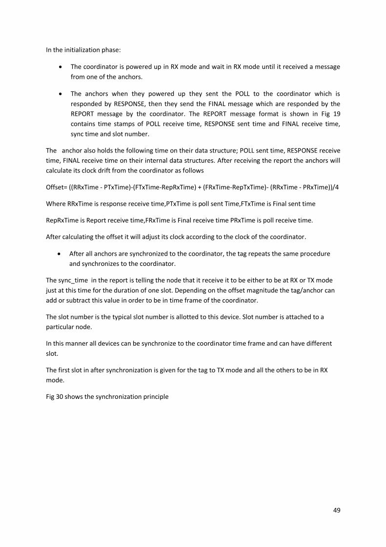
49

In the initialization phase:

The coordinator is powered up in RX mode and wait in RX mode until it received a message

from one of the anchors.

The anchors when they powered up they sent the POLL to the coordinator which is

responded by RESPONSE, then they send the FINAL message which are responded by the

REPORT message by the coordinator. The REPORT message format is shown in Fig 19

contains time stamps of POLL receive time, RESPONSE sent time and FINAL receive time,

sync time and slot number.

The anchor also holds the following time on their data structure; POLL sent time, RESPONSE receive

time, FINAL receive time on their internal data structures. After receiving the report the anchors will

calculate its clock drift from the coordinator as follows

Offset= ((RRxTime - PTxTime)-(FTxTime-RepRxTime) + (FRxTime-RepTxTime)- (RRxTime - PRxTime))/4

Where RRxTime is response receive time,PTxTime is poll sent Time,FTxTime is Final sent time

RepRxTime is Report receive time,FRxTime is Final receive time PRxTime is poll receive time.

After calculating the offset it will adjust its clock according to the clock of the coordinator.

After all anchors are synchronized to the coordinator, the tag repeats the same procedure

and synchronizes to the coordinator.

The sync_time in the report is telling the node that it receive it to be either to be at RX or TX mode

just at this time for the duration of one slot. Depending on the offset magnitude the tag/anchor can

add or subtract this value in order to be in time frame of the coordinator.

The slot number is the typical slot number is allotted to this device. Slot number is attached to a

particular node.

In this manner all devices can be synchronize to the coordinator time frame and can have different

slot.

The first slot in after synchronization is given for the tag to TX mode and all the others to be in RX

mode.

Fig 30 shows the synchronization principle

50

RX

TX

P

coordinator

Anchor1

TX

R

R

X

TX

F

R

X

TX

R

P

R

XSleep

TX

PAnchor2

R

X

TX

F

R

XSleep

R

X

TX

R

R

X

TX

R

P

RXTX

R

R

X

TX

R

P

TX

P

R

X

TX

F

R

XSleepAnchor3

RXTX

R

R

X

TX

R

P

TX

P

R

X

TX

F

R

XSleep

Sync-Time

RX

R

X

R

X

R

X

TX

TD

R

X

TX

TD

TX

TD

TX

TD

Sl

ee

p

Sleep

Sleep

Sleep

Sleep

Time

Tag

Figure 30:Synchronization

In the figure TXP is TX poll,TXR is TX response,TXF is TXFinal,and TXTD is TXTDOA.After all the devices

are synchronized the data transfer phase can continue ,but since we calculate the position using

TDOA and our transceiver clock has a drift of 2PPM(Parts per million) they are needed to be

synchronized by 0.1ns between the clocks of the coordinator and the . Since the micro-controller in

the TAG has memory requirements so the resynchronization method that is used here predicts when

they are going to be out of synchronization using Moving Average Drift Compensation (MADC)[19].In

our implementation it is assumed that the minimum amount of time they lose synchronization is

1sec initially. Using MADC formula the offset can be predicted as in eq(5.1).

C Pre _avarage(t)=αCpre +(1-α) C Pre _avarage(t-1)-------------(4.2)

Where C Pre _avarage(t) is the next predicted time where the lose synchronization,

C Pre _avarage(t-1) is the current predicted time,

α is waiting factor =0.1

It is outside of the scope of this thesis work to implement a more efficient synchronization algorithm.

4.4.3.2 TDOA Transfer phase

Once the synchronization completes the next phase is TDOA transfer phase. The vertical line

(Sync_Time) in Fig 23 differentiates the synchronization phase from the TDOA phase.

In TDOA transfer phase i.e. just after the Sync_Time all the anchors and the coordinators will be in RX

mode, but the tag will broadcast TDOA which is received by the coordinators and all anchors and

then go to sleep until it reaches it is next slot for transmission.

Each anchors and coordinator will record the time that they receive the TDOA message from the tag.

51

Each anchors that receive this TDOA message transmit this message to the coordinators by

piggybacking the receive time of TDOA message to the coordinator when their slot for transmission

reaches.

The coordinator will be on RX mode until it receives all TDOA message from the three anchors and

pass the time stamps from each anchors payloads and its own timestamp to the position server.

If any device in the system loses synchronization, then it can resynchronize again and it will be assign

a new time where it catch the all the communication again.

Fig 31 and Fig 32 shows the TDOA transfer and resynchronization in the data transfer phase.

RXcoordinator

Anchor1R

X

Anchor2R

X

Anchor3

Time

Tag

Sync-Time

Sync-Phase TDOA transfer-Phase

R

X

TX

TD

Slee

p

TX

TDSleep

SleepTX

TDSleep

SleepTX

TD

Sleep

Sleep

4TDOA Received

Transmit to server

1sec

RX

R

X

Slee

p

TX

TDSleep

R

XSleep

TX

TDSleep

R

XSleep

TX

TDSleep

TX

TDSleep

Figure 31: TDOA transfer

In Fig 32 it is shown that anchor 3 loses its synchronization, and then it waits until it slot time is

reached and synchronizes to the coordinator. If any resynchronization comes the coordinator will

discard all the TDOA message it received and start to receive again.

52

RXcoordinator

Anchor1R

X

Anchor2R

X

Anchor3

Time

Tag

Sync-Time

Sync-Phase TDOA transfer-Phase

R

X

TX

TD

Slee

p

TX

TDSleep

SleepTX

TDSleep

SleepTX

TD

Sleep

Sleep

Receive Poll

It will send Response

1sec

RX

R

X

Slee

p

TX

TDSleep

R

XSleep

TX

TDSleep

R

XSleep

TX

TDSleep

TX

TDSleep

TX

P

R

X

TX

F

R

X

Losses

Synchronization

TX

RRX

TX

R

P

Figure 32: Resynchronization

4.4.4 Measurement Results

Since the connection between the coordinator and the position server (Ethernet cable) is not yet

implemented, I only see the packet that is reaching to the coordinator and transmitted by the

coordinator using UART (Universal Asynchronous Receiving /transmitting) Interface in the serial COM

port. Table 9 shows this message exchanges and the initial measurement.

The measurements are done the same room .As can be seen in the table the time it takes for the

anchors/tag to be initialized/synchronized are different. This arises due to fading, interference and to

some extent clock offset drift .This can be shown in the table by comparing the number of timeouts

in RESPONSE/REPORT for each anchor.

Once they are synchronized; the next phase is TDOA phase.

In TDOA Phase:

1. The Tag simply broadcast its TDOA message.

2. All anchors and coordinator should receive the TDOA message from the tag, but the arrival

time of the TDOA message to all this nodes is different.

3. The anchors each waits for their slots and transmit the message to the coordinator.

4. After receiving all the TDOA message the coordinator will transfer to the position server

(when the system is launched)

53

5. In any case if one device loses its synchronization, then it will resynchronize to the

coordinator and the coordinator will start to receive the TDOA message from the tag.

Device Name/ID

Coordinator Side: Message Received(RED)/Message

Transmitted (Blue) PHASE PHASE

Anchor/1 POLL RESPONSE POLL RESPONSE POLL RESPONSE POLL RESPONSE FINAL REPORT

RESPONSE DELAYED INTIALIZED

INTIALIZATION

Anchor/2 POLL RESPONSE FINAL REPORT INTIALIZED

Anchor /3 POLL RESPONSE POLL RESPONSE POLL POLL RESPONSE FINAL REPORT POLL RESPONSE POLL RESPONSE POLL POLL RESPONSE FINAL REPORT

RESPONSE DELAYED REPORT DELAYED RESPONSE DELAYED INTIALIZED

INTIALIZATION

Tag POLL RESPONSE FINAL REPORT POLL RESPONSE POLL RESPONSE POLL POLL RESPONSE POLL RESPONSE POLL RESPONSE FINAL REPORT POLL RESPONSE FINAL REPORT

REPORT DELAYED RESPONSE DELAYED RESPONSE DELAYED REPORT DELAYED INTIALIZED

INTIALIZATION

Tag TDOA(1) TDOA

Anchor/1 TDOA(2) TDOA



Coordinator have receive 4 time stamps ,now it can send them to the position server Here actual Distance is 2.5 m from the coordinator, but the measured distance coordinates are (2.09m, 3.11m) =3.745m in radius.

After 1 sec the tag can send the TDOA message again

Tag TDOA(1)

Anchor/1 TDOA(2)

Anchor/3 POLL RESPONSE POLL RESPONSE POLL RESPONSE POLL RESPONSE POLL RESPONSE FINAL REPORT

ANCHOR 3 LOSSES SYNCHRONZARION SYNCHRONIZED

SYNCHRONIZATION

Since a new synchronization comes in the middle, the coordinator will delete the previously received TDOA and will start to expect a new one from the tag and all the others received in the middle will be ignored.

Tag TDOA(1) TDOA




Coordinator have receive 4 time stamps ,now it can send them to the position server Here actual Distance is 2.9 m from the coordinator, but the measured distance coordinates are (2.11m, 3.23m) =3.858m in radius. Table 9: localization Measurement Result

From table 9, we can see that the tow measured values are within the deviation of 1.10m which is

the result of delayed time for the network to initialize and resynchronize. This measurement can be

further improved by making the network to synchronize very efficiently.

54

5. Conclusion and Future Work

5.1 Conclusion

In this project, an indoor positioning system based on IEEE 802.15.4a system is designed and

implemented. The thesis report presents an overview and comparison of the current technologies

that is used in such systems ,it also describes how ranging and localization can be achieved in indoor

environment , and finally it also discusses the available MAC layer protocols for WSN and how the

choice of the MAC layers were made with respect to our system.

From the available indoor positioning technologies UWB is chosen because of its low power

consumption, precise positioning and robustness to fading and interferences.

The implementation and evaluation contains two parts

The peer-to-peer implementation and evaluation

Implementation of the system that contains 1 coordinator, 1 tag and 3 anchors (Scaled

System considering the MAC and PHY layers).

The peer-to-peer evaluation shows that the UWB system can measure a distance to an accuracy level

up to ± 15 cm in LOS, but this accuracy drops to ±50 cm in NLOS environment.

The peer-to-peer implementation has a fairly good precision of with 90% probability of being with in

the range of ±25cm when the mobile device (tag) moves with in LOS, but when the tag is moving in

NLOS area we have noticed that the this probability decreased to 50% of the required range of

±50cm.From we conclude that this drop in accuracy is due to signal delay and interferences occur

between the sender and the receiver.

In the implementation of the second system (scaled system) we have seen the time it requires for a

node to get into the network (initialization) phase can varies from node to node, and to get an

accuracy of ±30cm we must achieve synchronization of 0.1ns, it is a very difficult task to achieve this

wirelessly and no previous work has been found for UWB technology who have implement this. Since

the connection between the coordinator and the position server has not implemented to this date

(07/01/13) so we cannot measure the accuracy of the distance measurement, but I have tried to

calculate the distance from the received timestamp (using eq 3.3) and the calculation shows the

deviation is within the range of ±1.1m, this can be further improved by having good synchronization.

The expected battery is not achieved because the transceiver IC that we have at the moment doesn’t

support the sleeping mode, so we are forced to use Idle mode which has power consumption (8mA)

by itself this does not leave enough time for the capacitor to charge to the required value, so now we

have reached only 10-15 min batter life.

5.2Future Work

This section presents the issues which needed to be addressed in order to improve the performance

of the system.

55

The MAC layer protocol that we have implemented should be scaled and tested in large

network to maintain robustness.

If the transceiver IC supports SLEEP mode, in the future we can try to achieve battery life of

up to 5 years can be achieved.

Since the major power consumption of the transceiver IC lays in idle listening of PREAMBLE,

so if we adjust its length by considering the measurement of the distance, we can even

increase the battery life more.

Developing the upper protocol stacks, network and application layer for anchors and

coordinator.

56

Bibliography

[1]. Xin-long Luo, Wei Li, and Jia-ru Lin, “Geometric Location Based on TDOA for Wireless Sensor

Networks,” ISRN Applied Mathematics, vol. 2012, Article ID 710979, 10 pages, 2012.

doi:10.5402/2012/710979

[2]. Benoit Denis, “ UWB Localization Techniques, “In support of TG4a Ranging Subcommittee work,

IEEE P802.15 working group for WPAN, doc:IEEE802.15-04/418vo,August ,2004.

[3]. R. Roberts, “TDOA Localization Techniques,” In support of TG4a Ranging Subcommittee work,

IEEE P802.15 working group for WPAN, IEEE 802-15-04-0572-004a, October, 2004.

[4 IEEE 802.15.4a Task Group 4 (TG4), [online]: Available: http://www.ieee802.org/15/pub/TG4.html.

Last Accessed: Nov 14, 2012.

[5].IEEE 802.15.4a WPAN Low Rate Alternate PHY Task Group 4a (TG4a), [online]: Available:

http://www.ieee802.org/15/pub/TG4a.html. Last Accessed: Jan 2, 2013

[6]. Z. Jinyun Zhang, P.V. Orlik, Z. Sahinoglu, A.F. Molisch, P. Kinney, "UWB Systems for Wireless

Sensor Networks," Proceedings of the IEEE , vol.97, no.2, pp.313-331, Feb. 2009

[7]. Ilker Demirkol, Cem Ersoy, and Fatih Alagöz, “MAC Protocols for Wireless Sensor Networks: a

Survey,” IEEE Communications Magazine, pp.115-121, April 2006.

[8]. Joseph Kabara and Maria Calle, “MAC Protocols Used by Wireless Sensor Networks and a

General Method of Performance Evaluation,” International Journal of Distributed Sensor Networks,

vol. 2012, Article ID 834784, 11 pages, 2012. doi:10.1155/2012/834784.

[9]. Y. Al-Obaisat and R. Braun,” Wireless Sensor Networks: Architectures. Protocols, Applications,

and Management,” Auswireless Conference, 2006

[10]. H. Karl, A. Willig, “Protocols and Architectures for Wireless Sensor Networks,” John Wiley &

Sons, New York, 2005.

[11].G. Lu, B. Krishnamachari, and C. S. Raghavendra, “An Adaptive Energy-Efficient and Low-Latency

MAC for Data Gathering in Wireless Sensor Networks,” Proc. 18th Int’l. Parallel and Distrib.

Processing Symp., Apr. 2004, p. 224.

[12]. P. Lin, C. Qiao, and X. Wang, “Medium Access Control with a Dynamic Duty Cycle for Sensor

Networks,” IEEE WCNC, vol. 3, Mar. 2004, pp. 1534–39.

[13]. “Comparison of Wireless Indoor Positioning Technologies,” whitepaper, Ekahau Inc, 2000-2006

[14].Rilind Ballazhi, “Wireless Indoor Positioning Techniques,” Communication Systems V. IFI

Technical Report, IFI 2012.06, pages 55-67, August 2012.

[15].Tingcong Ye, Michael Walsh, Peter Haigh, John Barton, Alan Mathewson, Brendan O’Flynn,

“Experimental Impulse Radio IEEE 802.15.4a UWB Based Wireless Sensor Localization Technology:

Characterization, Reliability and Ranging,” technical report, Tyndall national institute, June, 2011.

http://www.ieee802.org/15/pub/TG4.html

http://www.ieee802.org/15/pub/TG4a.html

57

[16]. Zigbee Alliance [online]: Available at

http://www.zigbee.org/About/AboutTechnology/ZigBeeTechnology.aspx: Last Accessed: Dec 14,

2012

[17]. Zafer Sahinoglu, Sinan Gezici, “Ranging in the IEEE 802.15.4a Standard TR2006-0 97”, December

2006.

[18]. Rainer Mautz,” Indoor Positioning Techniques,” habilitation thesis, ETH-Zurich, Feb 2012

[19]. M. Brzozowski, H. Salomon, and P. Langendoerfer, “On efficient clock drift prediction means

and their applicability to IEEE 802.15.4,” in Proceedings of the IEEE/IFIP 8th International Conference

on Embedded and Ubiquitous Computing (EUC '10), pp. 216–223, December 2010

http://www.zigbee.org/About/AboutTechnology/ZigBeeTechnology.aspx

Documents

Implementation of Indoor Positioning using …603894/FULLTEXT01.pdf · Implementation of Indoor Positioning using ... of indoor positioning like WIFI, ... to the level of ±30 cm