Embed Size (px)
Citation preview

Louisiana State UniversityLSU Digital Commons
LSU Master's Theses Graduate School
2002
Implementation of an integrated quality assuranceprogram for CT-TPS processJunqing WuLouisiana State University and Agricultural and Mechanical College, [email protected]
Follow this and additional works at: https://digitalcommons.lsu.edu/gradschool_theses
Part of the Physical Sciences and Mathematics Commons
This Thesis is brought to you for free and open access by the Graduate School at LSU Digital Commons. It has been accepted for inclusion in LSUMaster's Theses by an authorized graduate school editor of LSU Digital Commons. For more information, please contact [email protected].
Recommended CitationWu, Junqing, "Implementation of an integrated quality assurance program for CT-TPS process" (2002). LSU Master's Theses. 2866.https://digitalcommons.lsu.edu/gradschool_theses/2866

IMPLEMENTATION OF AN INTEGRATED QUALITY ASSURANCE PROGRAM
FOR A CT-TPS PROCESS
A Thesis
Submitted to the Graduate Faculty of the Louisiana State University and
Agricultural and Mechanical College In partial fulfillment of the
Requirements for the degree of Master of Science
in
The Department of Physics and Astronomy
By Junqing Wu
B.S. in Nuclear Physics and Nuclear Technology Peking University, 2000
December, 2002

ii
ACKNOWLEDGEMENTS
I would like to express my sincere appreciation to my advisor, Dr. Oscar Hidalgo,
who has given me great advice and help in the whole process of my thesis.
I am grateful to my committee members for their helpful advice: Dr. Mark
Williams, Dr. Erno Sajo and Dr. Shelden Johnson.
I would also like to thank Dr. Thomas Kirby, Dr. William Bice, Angela Stam, and
Denis Neck for their generous advice on both my thesis research and routine work.
I would like to thank Pat Summers, Eddie Singleton and Chad Dunn for their kind
help with the treatment planning computers and Doug Nedan with CT-simulator
operations. My thanks also go out to all the friends at Mary Bird Perkins Cancer Center.
Without your help, it would have been impossible for me to have completed my thesis
research work.
I also want to thank my host parents, John Keady and Kaye Keady. Thank for
their help on both my living and their kind correction of this thesis.
My parents and sister also have my deepest thanks for their support and love in
spite of the great distance separating us.
Finally, I would like to express my gratitude to my girlfriend, Yuhong Sheng who
supports me with love and patience.

iii
TABLE OF CONTENTS
ACKNOWLEDGEMENTS. ............................................................................................ ii
LIST OF TABLES…………. .......................................................................................... vi
LIST OF FIGURES……….. ........................................................................................... ix
ABSTRACT………………….......................................................................................... xi
CHAPTER 1. INTRODUCATION ................................................................................. 1 1.1 Treatment Planning Process...................................................................................... 1 1.2 Treatment Planning System ...................................................................................... 2 1.3 Acceptance Test of TPS............................................................................................ 2 1.4 Commissioning of TPS............................................................................................. 3 1.5 Quality Assurance (QA) ........................................................................................... 3 1.6 Why TPS QA ............................................................................................................ 3 1.7 QA at Mary Bird Perkins Cancer Center (MBPCC)................................................. 5 1.8 Summary ................................................................................................................... 5
CHAPTER 2. LITERATURE REVIEW........................................................................ 6 2.1 The TG-40................................................................................................................. 6 2.2 The TG-53................................................................................................................. 6 2.3 Lecture by Van Dyke in 2001 AAPM Annual Meeting ........................................... 8 2.4 Documentation Requirement .................................................................................... 9 2.5 Other Works............................................................................................................ 10 2.6 Summary ................................................................................................................. 10
CHAPTER 3. GLOBAL METHODOLOGY............................................................... 12 3.1 Procedure ................................................................................................................ 12 3.2 Schedule.................................................................................................................. 13 3.3 Criteria for Acceptability ........................................................................................ 13 3.4 Software Upgrade ................................................................................................... 14 3.5 Summary ................................................................................................................. 15
CHAPTER 4. CT- PINNACLE3 QA............................................................................. 16 4.1 Introduction............................................................................................................. 16
4.1.1 What is Pinnacle3 ............................................................................................. 16 4.1.2 Pinnacle3 Algorithms ....................................................................................... 16
4.2 Methodology........................................................................................................... 18 4.2.1 Check Sum Program ........................................................................................ 18 4.2.2 Reference Cases ............................................................................................... 19 4.2.3 QA Plan Making .............................................................................................. 22

iv
4.2.4 Comparison...................................................................................................... 23 4.2.5 Digitizer QA in Pinnacle3 ................................................................................ 28 4.2.6 Criteria of Acceptability .................................................................................. 28 4.2.7 Documentation of Pinnacle3 ............................................................................ 29 4.2.8 Test Frequency................................................................................................. 29 4.2.9 Annual Pinnacle3 QA (or Recommissioning) .................................................. 29 4.2.10 Pinnacle3 Individual Test ............................................................................... 30 4.2.11 Software Upgrade Test .................................................................................. 30
4.3 Result and Analyses................................................................................................ 31 4.3.1 Checksum......................................................................................................... 31 4.3.2 Reference Case Comparison ............................................................................ 31
4.3.3 Digitizer Test…………………………………………………………………36 4.3.4 Pinnacle3 Individual Test ................................................................................. 37 4.3.5 Software Upgrade ............................................................................................ 37
4.4 Discussion ............................................................................................................... 38 4.4.1 Checking of Data Transfer from CT to Pinnacle3 by Checksum Program...... 38 4.4.2 Pinnacle3 IMRT Planning Repeat Test ............................................................ 39 4.4.3 Accuracy of DRR (Digital Reconstructed Radiographs)................................. 39 4.4.4 Pinnacle3 and CT Tape Saving Test................................................................. 39 4.4.5 Impractical Implementation of Treatment Plan ............................................... 39 4.4.6 Other Tests ....................................................................................................... 40
4.5 Conclusion .............................................................................................................. 40
CHAPTER 5 CT-SIMULATOR QA ............................................................................ 41 5.1 Introduction............................................................................................................. 41
5.1.1 CT-Simulator History ...................................................................................... 41 5.1.2 CT-Simulator Principle.................................................................................... 41 5.1.3 MBPCC Situation ............................................................................................ 42
5.2 Literature Review.................................................................................................... 42 5.3 Methodology........................................................................................................... 45
5.3.1 Physical Density to CT Number Conversion Consistence .............................. 45 5.3.2 Ongoing CT QA............................................................................................... 46 5.3.3 QA Equipment ................................................................................................. 46
5.3.4 Daily QA……………………………………………………………………...48 5.3.5 Weekly QA ...................................................................................................... 48 5.3.6 Monthly QA..................................................................................................... 50 5.3.7 Annual QA....................................................................................................... 51 5.3.8 Physical Density to CT Number Calibration ................................................... 54
5.4 Result ...................................................................................................................... 55 5.4.1 CT Number Consistence .................................................................................. 55 5.4.2 QA Measurement Summary ............................................................................ 55 5.4.3 Noise Variation ................................................................................................ 55
5.5.4 High Contrast Spatial Resolution……………………………………………..59 5.4.5 Dose and Performance for CT-Simulator Tube ............................................... 59 5.4.6 Physical Density to CT Number Conversion Table......................................... 60
5.5 Discussion ............................................................................................................... 60

v
5.5.1 Mechanical Test ............................................................................................... 60 5.5.2 Laser Checking Frequency…………………………………………………...63
5.6 Conclusion .............................................................................................................. 63
CHAPTER 6 VARIAN VARISEED 6.7 QA ................................................................ 64 6.1 Introduction............................................................................................................. 64 6.2 Literature Review.................................................................................................... 64 6.3 Methodology........................................................................................................... 64
6.3.1 Reference Treatment Plan................................................................................ 65 6.3.2 Dose Calculation Verification Test Using a Dose Point.................................. 66 6.3.3 Dose Calculation Verification Test Using Isodose Contours .......................... 68 6.3.4 DVH and CVA Results Test ............................................................................ 69
6.4 Result……………………………………………………………………………...70 6.4.1 Reference Treatment Plan Comparison ........................................................... 70 6.4.2 VariSeed Internal Test Procedure .................................................................... 71
6.5 Discussion ............................................................................................................... 71 6.6 Conclusion………………………………………………………………………...76
CHAPTER 7. PLATO-BRACHYTHERAPY TPS QA............................................... 77 7.1 Introduction............................................................................................................. 77 7.2 Methodology........................................................................................................... 78
7.2.1 Reference Case................................................................................................. 78 7.2.2 Software Calculation Test................................................................................ 79 7.2.3 Digitizer Test ................................................................................................... 79 7.2.4 Checksum Test................................................................................................. 80 7.2.5 Output Check ................................................................................................... 80 7.2.5 Verification Frequency .................................................................................... 80
7.3 Result and Analyses................................................................................................ 80 7.3.1 Tandem & Ring Case....................................................................................... 80 7.3.2 Vagina Cylinder Case ...................................................................................... 81 7.3.3 Digitizer Test ................................................................................................... 84
7.4 Discussion ............................................................................................................... 84 7.5 Conclusion .............................................................................................................. 86
CHAPTER 8. GLOBAL DISCUSSION ....................................................................... 87 8.1 Test of Whole Radiation Treatment Process .......................................................... 87 8.2 Test from Treatment Planning Computers to the LINACS .................................... 88
CHAPTER 9. GLOBAL CONCLUSION..................................................................... 92
REFERENCES………………........................................................................................ 93
VITA………………………............................................................................................. 96

vi
LIST OF TABLES
Table 2.1 TG-40 recommendations on the frequency of treatment planning computers QA………………............................................................................................ 7
Table 3.1 Dose calculation criteria recommended by J. Van Dyk.............................. 14
Table 4.1 Pinnacle3 QA Phantom CT-scan parameters .............................................. 19
Table 4.2 DVH data table for organ_2 in 21EX(BR) reference plan ......................... 26
Table 4.3 Recommendation on the criteria of TPS QA............................................... 28
Table 4.7 Monitor Unit per fraction comparison in 21EX(BR) QA plans ................ 35
Table 4.4 Point dose comparison (1) between 21EX(BR) reference plan and QA plan………………………….. ......................................................................................... 32
Table 4.5 Point dose comparison (2) between 21EX(BR) reference plan and QA plan……………………………....................................................................................... 32
Table 4.6 Point dose comparison (3) between 21EX(BR) reference plan and QA plan……………………………....................................................................................... 32
Table 4.8 Dimension measurement on Monitor Display and printout compared to the caliper measurement……… .................................................................................... 36
Table 4.9 Points coordinate comparison in digitizer test ............................................ 36
Table 4.10 Length measurement comparison in digitizer test.................................... 36
Table 4.11 Dose comparison in Pinnacle3 individual test............................................ 37
Table 4.12 Point dose comparison after Pinnacle3 software upgrade ........................ 38
Table 5.1. Summary of CT-Simulator QA at MKSCC ............................................... 44
Table 5.2 CT scan technique of ADAC QA Phantom.................................................. 46
vii
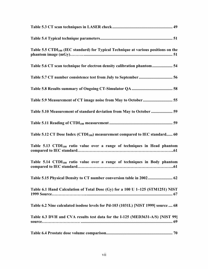
Table 5.3 CT scan techniques in LASER check........................................................... 49
Table 5.4 Typical technique parameters....................................................................... 51
Table 5.5 CTDI100 (IEC standard) for Typical Technique at various positions on the phantom image (mGy)………........................................................................................ 51
Table 5.6 CT scan technique for electron density calibration phantom.................... 54
Table 5.7 CT number consistence test from July to September ................................. 56
Table 5.8 Results summary of Ongoing CT-Simulator QA ........................................ 58
Table 5.9 Measurement of CT image noise from May to October............................. 55
Table 5.10 Measurement of standard deviation from May to October ..................... 59
Table 5.11 Reading of CTDI100 measurement .............................................................. 59
Table 5.12 CT Dose Index (CTDI100) measurement compared to IEC standard...... 60
Table 5.13 CTDI100 ratio value over a range of techniques in Head phantom compared to IEC standard……………………………………………………………..61
Table 5.14 CTDI100 ratio value over a range of techniques in Body phantom compared to IEC standard……………………………………………………………..61
Table 5.15 Physical Density to CT number conversion table in 2002........................ 62
Table 6.1 Hand Calculation of Total Dose (Gy) for a 100 U 1–125 (STM1251) NIST 1999 Source……………………...................................................................................... 67
Table 6.2 Nine calculated isodose levels for Pd-103 (1031L) [NIST 1999] source .... 68
Table 6.3 DVH and CVA results test data for the I-125 (MED3631-A/S) [NIST 99] source………………………. .......................................................................................... 69
Table 6.4 Prostate dose volume comparison................................................................. 70

viii
Table 6.5 Prostate volume dose comparison................................................................. 70
Table 6.6 Dose Calculation Verification Test Result Summaries............................... 72
Table 6.7 DVH and CVA Test Result Summary.......................................................... 75
Table 7.1 Initial dose rate comparison in Tandem & Ring case................................. 81
Table 7.2 Point Coordinate comparisons in Tandem & Ring case............................. 81
Table 7.3 Point dose comparison in Vagina Cylinder case ......................................... 82
Table 7.4 Absolute time comparison after correction by decay factor ...................... 82
Table 7.5 Point coordinate comparison in Vagina Cylinder case............................... 84
Table 7.6 Point dose comparison in software calculation test .................................... 84
Table 7.7 Digitizer test in PLATO Brachytherapy planning system (Unit: cm)....... 85

ix
LIST OF FIGURES
Figure 1.1 Flowchart of radiation treatment process .................................................... 2
Figure 4.1 QA phantom connected to CT couch.......................................................... 20
Figure 4.2 Example of dose profile in the output of ADAC........................................ 24
Figure 4.3 Example of DVH provided by Pinnacle3 .................................................... 25
Figure 4.4 (1) (2) (3) Point dose comparison between 21EX(BR) reference plan and QA plan………………………….................................................................................... 33
Figure 5.1 Three sections of CT QA phantom ............................................................. 47 Figure 5.2 CT QA phantom connecting to CT couch………………………………...47
Figure 5.3 WILKE Phantom.......................................................................................... 49
Figure 5.4 The measurement position of CTDI100........................................................ 52
Figure 5.5 Body phantom for CTDI100 measurement.................................................. 52
Figure 5.6 Head Phantom for CTDI100 measurement ................................................. 53
Figure 5.7 CTDI100 measurement setup........................................................................ 53
Figure 5.8 CIRS Model 62 electron density calibration phantom.............................. 54
Figure 5.9 CT# consistence comparison (1) from July to September ........................ 57
Figure 5.10 CT# consistence comparison (2) from July to September ...................... 57
Figure 5.11 Noise Variation from May to September ................................................. 55
Figure 5.12 High Contrast Spatial Resolution Variation from May to October ...... 59
Figure 5.13 Physical density to CT number conversion table comparison in 2001 and 2002…………………………........................................................................................... 62

x
Figure 6.1 Dose calculation verification result using isodose lines............................. 74
Figure 7.1 Absolute time comparisons after correction of decay factor in Vagina Cylinder case………………. .......................................................................................... 83
Figure 8.1 RANDO phantom in treatment room......................................................... 88
Figure 8.2 Test result of whole treatment process. (The dotted line and solid line are calulation and measurement respectively).................................................................... 89
Figure 8.3 Test result from treatment planning computers to the LINACS............. 91

xi
ABSTRACT
Systematic constancy and accuracy of a treatment planning system (TPS) are
crucial for the entire radiation treatment planning process (TPP). The Quality Assurance
(QA) of individual components does not necessarily lead to satisfying performance of the
whole process due to the possible errors introduced by the data transfer process between
components and other fluctuations. However, most of current QA for TPS is confined to
the treatment planning computers. In this study, a time efficient and integrated CT-TPS
QA procedure is presented, which starts at the beginning of the TPS input --- Computer
Tomograhpy (CT). The whole QA procedure is based on the concept of simulating a real
patient treatment. Following the CT scan of a head phantom with geometrical objects, a
set of reference treatment plans for each accelerator, with all energy beams included,
were established. Whenever TPS QA is necessary, the same procedure is repeated and a
QA plan is produced. Through the comparison of QA plan with the reference plan, major
systematic errors can be found easily and quickly. This method was also applied to
VariSeed and PLATO Brachytherapy treatment planning systems.
Moreover, if any error is detected in the system, TPS is broken into several parts
and individual tests are also set up.

1
CHAPTER 1. INTRODUCATION
1.1 Treatment Planning Process
The treatment planning process usually involves beam data representation, patient
data acquisition, definition of treatment portals, dose calculations, dose display, dose
evaluation, and finally the plan documentation (Fraass et al. 1996)
First, the patient positioning and immobilization is set up. These position and
immobilization methods are going to be used when real treatment is ongoing.
Following that, the patient data is registered by Computed Tomography (CT).
Typically, CT images are acquired at transverse planes with a separation of 1 to 10 mm.
Based on these images, the physician can estimate the size, extent, and location of the
tumor. Sometimes, magnetic resonance imaging (MRI) and positron emission tomogrphy
(PET) are used to set up a more accurate patient model and particularly to improve the
accuracy of the tumor location. In some cases, the treatment fields and technique are
determined during the image acquisition.
The next step is treatment planning using a computer system. Treatment planning
computers get patient image data from the image acquisition equipments. Physicians and
dosimetrists delineate normal anatomic structures and the target volumes; add the beam
and beam modifiers; give the prescription and calculate the dose. After the plan
evaluation and approval by medical physicists and radiation oncologists, the treatment
plan is printed out as a hardcopy for patient treatment and records. The final plan is also
sent to the verify and record system (e.g. IMPAC) for patient treatment.
Finally, the plan is verified by additional radiographic imaging (e.g. port films)
before the dose is delivered to the patient.

2
Ultrasound
CT-Simulator
PET
MRI
ADAC LINACS
Digitizer HDR Machine Nucletron
Operation Room VariSeed
The whole process of the radiation therapy process can be illustrated in the
following flowchart:
Figure 1.1 Flowchart of radiation treatment process
Uncertainties or errors in any step of this process can have a significant effect on
the outcome.
1.2 Treatment Planning System
Basically, a treatment planning system (TPS) includes a computer workstation
and input and output devices for graphics and images. Further complex components of a
3D TPS are the dose calculation algorithm code and the program used to manipulate 3D
graphic displays of the patient, the beam geometry, and the dose.
1.3 Acceptance Test of TPS
An acceptance test is carried out to find out whether the TPS system performs
according to the manufacturer’s specifications. The objective is to know how the TPS
should perform in various situations.

3
1.4 Commissioning of TPS
Haken (1996) divided commissioning of a TPS into two parts, the nondosimetric
commissioning and dosimetric commissioning. Nondosimetric commissioning is used to
handle the TPS functions not directly related to the dose calculation. It is mainly TPS
dependent, and usually includes image acquisition, anatomical description, and beam
description. Dosimetric commissioning validates the dose calculation of a TPS. It
contains measured beam data input, defining dose calculation algorithm parameters and
verification of the calculation.
1.5 Quality Assurance (QA)
According to the definition of International Standards Organization (ISO), quality
assurance (QA) means all the planned or systematic actions necessary to provide
adequate confidence that a product or service will satisfy given requirements for quality.
Specifically in radiation oncology, the quality can be defined as the totality of
features or characteristics of the radiation oncology service that bear on its ability to
satisfy the stated or implied goal of effective patient care (G. Kutcher et al. 1994). QA of
radiation therapy equipment is primarily an ongoing evaluation of functional performance
characteristics. Quality assurance is essential to the safe and effective treatment of
patients, the analysis of data, and the design of prospective research.
1.6 Why TPS QA
In the entire radiation treatment process, the treatment-planning computer is a
crucial component, as it covers a wide range of applications. Since they are related to the
control of the disease or to complications as a result of inappropriate treatment, all of
these planned or systematic actions must be ensured working properly. Unlike treatment

4
delivery errors, which are usually random in nature, the errors from treatment planning
systems are more often systematic and constant for all the patient treatments. Also, no
system of computer programs is perfect, nor are the users of such programs error free.
The treatment planning computers are subject to electronic and mechanical failure.
With the rapid evolution of treatment planning systems, QA for treatment-
planning computers has lagged behind, especially after the introduction of 3-D treatment
planning system and the dynamic wedge. Medical physicists are challenged to ensure
that innovations in TPS and delivery systems meet agreed-upon standards for quality
assurance. The lack of proper TPS QA procedures has led to some serious accidents. An
example of the consequences of inadequate TPS QA is as follows.
In May 25, 2001, the International Atomic Energy Agency (IAEA) sent a team of
six international experts to assist the authorities of Panama to deal with the aftermath of a
radiological accident that occurred at Panama’s National Oncology Institute. In this case,
it was possible to enter data in one batch for several shielding blocks in different ways.
For some of these ways of entering the data, the output values were calculated
incorrectly. The consequence is that five patients died and the team confirmed that these
deaths were attributable to the patients' overexposure to radiation. Of the surviving 20
patients, about three-quarters of them developed serious complications, which in some
cases may ultimately prove fatal.
Also, TPS quality assurance is required by the American College of Radiology
(ACR). To be an ACR accredited institution, the TPS QA procedure must be setup and
performed regularly.

5
1.7 QA at Mary Bird Perkins Cancer Center (MBPCC)
At MBPCC, QA procedures for the treatment planning system have also fallen
behind. A 3-D treatment planning system was brought into MBPCC about 2 years ago,
but no quality assurance program has ever been set up or performed for Theraplan or
Pinnacle3. At the same time, TPS is used every day for almost all of our patients. If there
is any minor error, the cost would be unpredictable. With this motivation, a systematic
update of the QA procedure is required.
1.8 Summary
Treatment Planning System (TPS) QA is a vital requirement, even though
MBPCC is not as big as some huge cancer centers and has limited medical physicist
staffs. As TG-53 says, the quality assurance requirements in a small radiation oncology
facility should be no less than those in a large, academic medical center.
In this study, focus would be put on the Pinnacle3 external beam treatment
planning system QA.

6
CHAPTER 2. LITERATURE REVIEW
As for the significance of TPS, there are plenty of references available regarding
TPS Quality Assurance. To guide and help medical physicists in developing and
implementing a comprehensive but realizable program of quality assurance in treatment
planning system, the American Association of Physicists in Medicine (AAPM) organized
a Task Group 40 to summarize the essential points found in these literature. Later, due to
the importance and increasing sophistication and complexity of treatment planning
systems, the American Association of Physicists in Medicine (AAPM) Task Group report
53 was issued in 1998.
2.1 The TG-40
The TG-40 report (Comprehensive QA for Radiation Oncology) was published in
1994, when most institutions were still using 2-D treatment planning systems. Therefore,
this report is special for the 2-D treatment planning computers. Some of the
recommendations are already obsolete. However, it provides a basic idea about what to
check and how often it should be checked. The recommendations for the ongoing TPS
QA by the TG-40 report are shown in Table 2.1.
This report also points out that QA of treatment-planning systems is an evolving
subject. It keeps changing, and physicists need to keep up with the improvements.
2.2 The TG-53
In TG-53 (Quality Assurance for Clinical Radiotherapy Treatment Planning),
routine QA is also emphasized as being a very important part of the TPS QA program
after an initial commissioning of the dataset. According to the AAPM TG-53 report, the
main aims of a routine periodic QA program for RTP system include the following.

7
Table 2.1 TG-40 recommendations on the frequency of treatment planning computers QA
Frequency Test Tolerance Understand algorithm Functional Single field or source isodose distribution
2% or 2 mm
MU calculation 2% Test cases 2% or 2 mm
Commissioning and following software update
I/O system 1 mm Daily I/O devices 1 mm
Checksum No change Subset of reference QA test
set (when checksum not available)
2% or 2mm
Monthly
I/O system 1 mm
MU calculation 2% Reference QA test set 2% or 2 mm
Annual
I/O system 1 mm

8
First, the calculation algorithms of the TPS need to be tested periodically, relative
to the accuracy, precision, and limitations of the algorithm, as well as the implementation
of the software for isodose planning calculation and display. Most physicists may
understand the algorithm very well, but may not be aware of the software weaknesses.
After many years’ development, the algorithm tends to improve; therefore, although this
is still an important test, it is not as critical as it was previously.
Secondly, the correct functioning and accuracy of peripheral devices used for data
input need to be verified. These include the digitizer tablet, CT, MRI, video digitizer,
simulator control system, and devices to obtain mechanical simulator contours. One must
separately consider the devices themselves and the networks, tape drives, software,
transfer programs, and other components, which are involved in the information transfer
from the device to the TPS system.
The third objective is to confirm the integrity and security of the TPS data files
that contain the external beam and brachytherapy information used in dose and monitor
unit calculations.
Finally, it is necessary to confirm the function and accuracy of output devices and
software, including printers, plotters, automated transfer processes, connections to
computer-controlled block cutters and/or compensator makers, etc.
2.3 Lecture by Van Dyke in 2001 AAPM Annual Meeting
The latest report on TPS QA was given by Van Dyke in the 2001 AAPM annual
meeting. In this lecture, Van Dyke proposed the following items be checked after the
acceptance test and commissioning of TPS.
• Program and system documentation

9
• User training
• Sources of uncertainties
• Suggested tolerances
• Initial system checks (recommissioning)
• QC – repeated system checks
• QC – patient specific monitor unit checks
• QC – in vitro/vivo dosimetry
• QA – administration
Van Dyke also mentioned some challenges in QA testing. For example, is the 3-
D image information acquired and transferred accurately from the imaging device to the
treatment-planning computer? Does the treatment planning software provide accurate
reconstruction of the data provided by the imager?
2.4 Documentation Requirement
Documentation is an important part of the Quality Assurance procedure, but is
easy to be ignored. Dahlin et al. (1983) have proposed some basic documentation
requirements that should be available to the TPS user:
1. System description giving the general concepts of the system and the
hardware/software structure.
2. User’s guide giving a clear description for overall system usage.
3. Data file formats including a description of file contents.
4. Text file descriptions of communication files and how the user might edit such
files for local use.

10
5. Algorithm descriptions, which include a clear indication of the physical models
with all the relevant mathematical relationships and the corresponding levels of
accuracy. The system capabilities and program limitations should be clearly
outlined, preferably with an up-to-date list of scientific references. A detailed
description of dose normalization procedures should be included.
6. Device handlers must be described in the form of available libraries to ensure the
user access to available hardware peripherals.
7. Access to necessary software libraries including programmer handbooks for local
programming.
8. Basic data description of necessary basic data and how it is entered into the
system.
2.5 Other Works
Bruce Curran et al. (1991) suggested checking treatment-planning computers
using a reference plan, but their tests were limited to checking the computer itself. They
separately tested the input, treatment computers, and output devices. This made the QA
procedure extremely complex. Although they have simplified some individual test
procedures, the whole process was still too complicated.
2.6 Summary
Although the American Association of Physicists in Medicine (AAPM) has
published the TG-40 and TG-53 reports to guide physicists in performing treatment
planning system QA, both reports only give a framework. Neither describes details about
how to perform the TPS QA step-by-step. Moreover, TPS QA is a complicated task. It is
different from one clinic to another, since every clinic has its own special situations, e.g.

11
different treatment planning computers (TPC) and different facilities. As most medical
physicists have noticed, it is impossible and unrealistic to build a single set of procedures
and apply them to all situations. TPS QA procedures must be established based on each
institution’s own special situation.

12
CHAPTER 3. GLOBAL METHODOLOGY
3.1 Procedure
QA of treatment planning system is a comprehensive and systematic procedure
that involves consistency verification throughout the planning process from initial
localization on through to the output of treatment planning. Besides the establishment of
QA procedures, there are two points that need to be clear.
First, the input of external beam TPS is the CT-Simulator. Almost all of the
patient images are obtained from the CT-Simulator. It does not make sense only to check
the external beam TPS accuracy without the CT-Simulator working correctly. The
connection between the CT-Simulator and external beam TPS is DICOM (digital image
communication in medicine), which transfers the image series. This image transfer is
also an important part of the treatment planning process. Therefore, the TPS has to be
checked with the CT-simulator as a system.
Secondly, the TPS QA is an extremely time consuming and labor extensive work.
If all aspects of the TPS were checked, it would take more than one full time medical
physicist to complete it. In reality, it is costly and unnecessary. As recommended by the
AAPM TG-53 report, only selected points with possible errors need to be checked
routinely. Design of an appropriate QA program depends strongly on the planning
system capabilities and how these capabilities will be used clinically. It is extremely
important to incorporate the limitations of the planning system and its intended use
directly into the design of the QA procedures.
Because of the reasons above, we set up a procedure to test CT-TPS integration,
which is one of the points making our work different from others. Our integration QA

13
examines the systematic errors. After checking the integrity, the question is what should
be done if there is any error in the CT-TPS integration QA. Our way is to break the
integration and check ADAC and CT individually.
For the VariSeed 6.7 planning system and the PLATO Brachytherapy HDR
planning system, a similar method is used for the QA procedures. Some reference plans
were established to verify the systematic process accuracy. If any errors were found in
the QA, individual tests will be performed to check the devices separately.
3.2 Schedule
The schedule of the routine QA tests largely depends on the kinds of issues being
monitored. We need to know how often the feature is used in clinical procedures and
how critical this feature is. The TG-40 report gives a recommendation on the frequency
of routine QA. Our schedule will be based on that recommendation and the situation at
our institution.
3.3 Criteria for Acceptability
The International Commission of Radiation Units and Measurements (ICRU,
1978) have specified a tolerance of 2% in relative dose accuracy in low dose gradients or
2 mm spatial accuracy in regions with high dose gradients. For brachytherapy, the aim is
3% accuracy in dose at a distance of 0.5 cm or more, at any point for any radiation
source. However from the experience of many other cancer centers (Starkschall et al.
1998), this is an unrealistic goal, in spite of the extensive effort of developers for new or
improved dose calculation algorithms. Right now, the most popular criteria are proposed
by J. Van Dyk (1991) and widely accepted by most of medical physicists (Table 3.1).

14
Table 3.1 Dose calculation criteria recommended by J. Van Dyk Beam Photon Electron Density Distribution Homogeneous Heterogeneous Homogeneous HeterogeneousCentral ray data 2% 3% 2% 5% High dose, low gradient
3% 4% 4% 7%
Hi gradient 4mm 4mm 4mm 5mm Low dose, low gradient
3% 3% 4% 5%
In our QA test, it checks the reproducibility of the whole TPS, which is different
from the comparison between calculation and measurement. It is less strict because the
treatment planning system has more reliability and constancy. However, it is useless to
have an extremely small criterion because the error in the radiation treatment process
(RTP) is an accumulated error. If other parts of the treatment planning process introduce
greater errors, the whole RTP error would be still high. We have set our own criteria in
reference to the tolerance of dose calculation and the results obtained in our QA tests.
3.4 Software Upgrade
One of the most difficult parts of designing QA for TPS is to establish a
reasonable QA program for software upgrades. The full commissioning of a 3-D
treatment planning system may take up to several months or even longer; therefore it is
obviously not practical to perform such a full commissioning test on each new version of
the software. However, at the same time, it is well known that changes in the software
can lead to unintended and undesirable consequences in function and data. Old bugs may
be fixed, but new bugs may have been introduced. Testing must be performed to check
the accuracy.
The first thing for medical physicists to do after a software upgrade is to
understand what has been changed compared to the older version software. This needs to

15
be coordinated with the software manufacturer. Usually, the vendor of the software
provides a list of changes and new features in the software. The new features should be
tested and results should be documented.
In this study, the same ongoing TPS QA test procedures are also used to test the
software upgrade, but the test order is reversed. First, make a software individual test
without CT scan so as to check the changes of the treatment planning computers, instead
of the whole treatment process. If there were no significant change in the dose
calculation algorithm, the same result would be obtained. After that, the integrated QA
process can be used to assure that there is no change in the whole treatment planning
system.
3.5 Summary
The TPS-CT integrated test will be used for TPS QA by simulating the actual
patient treatment process. Also, TPS and TPS input individual QA will also be
established to check individual parts of the system when any error is found in the
integration test results. All of the tests are designed based on MBPCC specific situations.

16
CHAPTER 4. CT- PINNACLE3 QA
4.1 Introduction
4.1.1 What is Pinnacle3
Pinnacle3 is the external beam treatment planning system utilized at MBPCC,
which is provided by Philips ADAC Laboratories. The ADAC Pinnacle3 RTP system
runs on a Sun UNIX workstation with a Solaris operating system. The software supports
radiation therapy treatment planning for treatment of benign or malignant diseases.
4.1.2 Pinnacle3 Algorithms
4.1.2.1 Algorithm of Photon Beam Physics
Pinnacle3 uses the Collapsed Cone Convolution Superposition dose algorithm,
based on the work of Mackie, et al., 1985. The Collapsed Cone Convolution
Superposition dose model consists of three parts.
• Modeling the incident energy fluence as it exits the accelerators head.
• Projection of this incident energy fluence through the density representation of a
patient to compute a TERMA (Total Energy Released per unit Mass) volume.
• A three-dimensional superposition of the TERMA with an energy deposition
kernel to compute dose. A ray-tracing technique is also used during the
superposition to incorporate the effects of heterogeneities on lateral scatter.
The Pinnacle3 photon beam model parameters characterize the radiation exiting
the head of the linear accelerator by the starting point of a uniform plane of energy
fluence describing the intensity of the radiation. Then Pinnacle3 adjusts the fluence
model to account for the flattening filter, the collimators, and beam modifiers such as
blocks, wedges, and compensators.

17
4.1.2.2 Algorithms of Electron Physics
The Pinnacle3 electron dose calculation uses the Hogstrom pencil-beam algorithm
(Hogstrom et al. 1982). The algorithm uses a combination of measured data and model
parameters that characterize the electron beam physics. After determining the
appropriate electron model parameters, dose lookup tables are generated to use for dose
calculation.
4.1.2.3 Algorithm Accuracy
As recommended by TG-53 and other literature, the treatment planning system
algorithm needs to be tested. However, verifying the accuracy of the dose computation
requires a comprehensive set of test cases. The tests should include a lot of special
geometry cases, such as oblique incidence of the radiation beam (e.g. tangential breast
irradiation) or multiple density heterogeneities. Dose distributions can generally be
calculated very well for a radiation beam at normal incidence on a water phantom but
their accuracy in a variety of clinical situations is questionable.
The American Association of Physicists in Medicine (AAPM) Radiation Therapy
Committee Task Group 23 (TG-23) developed a test package for verifying the accuracy
of photon-beam dose-calculation algorithms. Data for the test cases were acquired for
two beam energies from two Clinical linear accelerators: a 4-MV x-ray beam from a
Clinna-4 (Varian Oncology Systems, Palo Alto, CA), and an 18-MV x-ray beam from a
Therac-20 (Atomic Energy of Canada, Ltd., Kanata, Ontario, Canada). However, it is a
time consuming and labor intensive job to complete all of these test cases.
Fortunately, with the help of Philips ADAC laboratory, M.D. Anderson Cancer
Center developed a more extensive set of measured data to verify the accuracy of the

18
photon dose-algorithm in Pinnacle3, which is the same treatment planning system used at
MBPCC (Starkschall et al. 1998). Their results show that the Pinnacle3 treatment
planning system calculated photon doses to within the American Association of
Physicists in Medicine (AAPM) Task Group 53 (TG-53) criteria for 99% of points in
buildup region and 90% of points in the penumbra. For the heterogeneous phantoms,
calculations agreed with actual measurements to within +/-3%. The monitor unit tests
revealed that the 18-MV open square fields, oblique incidence, oblique incidence with
wedge, and mantle field test cases did not meet the TG-53 criteria but were within +/-
2.5% of measurements.
The algorithm tests above required a whole team to complete the work at
considerable expense. It is impractical and unnecessary to repeat these test cases. In this
study, we utilize M. D. Anderson Cancer Center’s results and do not make further tests
on our own Pinnacle3 planning system.
4.2 Methodology
In this study, two methods were used to check the Pinnacle3 constancy and
accuracy.
4.2.1 Check Sum Program
Firstly, the “sum” program in the Unix system was used. This program calculates
and prints a 16-bit checksum signature for the named file, and also prints the number of
blocks in the file. It is typically used to look for bad spots or to validate a file
communication over transmission lines. Initially, all of the machines’ database files were
checked by the “sum” program and all the signatures (results) were stored as reference.

19
In the QA process, some of the files are selected and the signatures are spot-checked.
The result should be exactly the same as the reference plan.
One requirement for the use of checksum program is to follow the changes made
to the machine data. If the checksum result is different from the reference, we should be
able to find out the reason for the changes.
4.2.2 Reference Cases
Secondly, a series of reference plans starting from CT and ending up with
Pinnacle3 dose calculation were established. The whole QA process simulates the actual
patient treatment planning process. Detailed steps are as follows.
4.2.2.1 CT Scan of a Radiosurgery Heterogeneous Head Phantom
A radiosurgery heterogeneous head phantom was scanned by a CT scanner using
the most typical head scan technique parameters (See table 4.1). The phantom is
connected to the CT couch by a radiosurgery head phantom holder, as shown in Figure
4.1. After the first scan, a CT scan protocol was set up. The protocol bypasses the step
of image scouts, ensuring that the exact same scan technique is used each time. This also
reduces the total scanning time.
Table 4.1 Pinnacle3 QA Phantom CT-scan parameters Scan method KV mA Time Thickness Gantry Ang Total Slices
Helical 140 150 72 sec 3mm 0.0 48 Three B. B markers were put on the phantom aligning with the CT internal laser
in order to find out the same relative position in the image series scanned at different
times. Later, if the dose distribution needs to be measured in LINACS, B. B. markers can
also be used to align the LINACS lasers and find the isocenter point.

20
4.2.2.2 Transferring of Image Series to Pinnacle3
Within the CT computer network, the image series were sent to Pinnacle3 by
DICOM (Digital Image Communication in Medicine), which is widely considered as one
of the possible resources contributing to errors. Our QA test can catch this kind of errors
because the phantom images also go through this step. Were there any errors, it would
show up in the final treatment plan comparison.
Figure 4.1 QA phantom connected to CT couch
4.2.2.3 Saving Image Series as a Pinnacle3 Phantom
After importing the image series to the Pinnacle3, a new treatment plan was added
with the imported image series as the primary CT image series. In this new plan setup,
the laser point is defined as the point aligning with the B. B. markers. This is a very
important because all of the coordinates should be relative to the laser point in order to
keep all contours and POI in the same relatively positions. After exiting the treatment
planning, this plan was saved as a Pinnacle3 phantom named “QA HEAD PHANTOM”.

21
4.2.2.4 Transferring an Actual Patient Plan Technique
Different plans were devised for different machines.
For the 21EX(Baton Rouge) and 21EX(Covington), they have Multiple Leaves
Collimator (MLC) and Intensity Modulation Radiation Treatment (IMRT) can be applied.
Thus an actual head tumor patient IMRT treatment plan with 6 beams (256 Brain, 180
Brain, 95 Brain, LSO Brain, VERTEX Brain, and RSO Brain) was selected and copied to
the “QA HEAD PHANTOM”. Some new contours and points of interest (POI) were
added. The contours included critical organs in order to check the DVH calculation.
Most of POIs are around the tumor or in the high gradient dose region. If either the
image position or computer calculations have errors, the dose change would be relatively
larger and more easily observed.
For the other three machines (2100C, 600C and 2000CR), an actual patient 3-D
conformal head tumor treatment plan was transferred to the “QA HEAD PHANTOM”.
This plan included blocks, wedges and boost beams, which allow us to test all of these
characteristics. After transferring, some contours and POIs were also added to the plan.
There are two advantages to transfer the treatment plan technique. First, a whole
treatment plan technique can be transferred to “QA HEAD PHANTOM”, resulting in no
need to add all the beams, plot blocks, contour organs, defined POI, and so on. This
saves a huge amount of time and it is one of the reasons that the TPS QA in this study can
be completed much more quickly than other work. Secondly, all of the treatment
parameters can be kept the same. Without transferring, many parameters, like the block
shape, calculation grids and contour shapes are very difficult or even impossible to be

22
kept in the exactly same. The treatment plan transferring is the key of all of our TPS QA
procedures.
4.2.2.5 Dose Calculation and Printout
The dose distribution was calculated with the Adaptive Convolve Method, which
is the most common method used by dosimetriests. Following that, the treatment plan
report, DVH, DRR, three 2-D isocenter plane images and isodose distribution for every
three slices were all printed out. All of these printouts are in keeping with how
dosimetrists typically operate and provided as a treatment plan to physicians. The correct
printout shows us the TPS output devices are working properly.
4.2.3 QA Plan Making
Whenever a TPS QA is necessary, we will repeat the generation of the reference
plan and make a QA plan. Then the QA plan result was compared to the reference plan
result. If the Pinnacle3 and CT integration TPS has been working consistently, the QA
plan result should be the same or only slightly different from the reference plan. A QA
treatment plan is generated in manner very similar to the reference plan---scan the
phantom in the same position, transfer the images, save them also as “QA HEAD
PHANTOM”, and calculate the dose distribution. But there are also some differences as
follows.
First, transfer the reference plan instead of actual patient plan to the QA plan. In
this way, the QA plan can be initialized with all of the beams, contours, points,
prescriptions, blocks, wedges and grids already included in the reference plan.
Secondly, the alignment point of transferring the reference plan should be the new
ISO at the new phantom image series. To find the coordinates of the new ISO, it is

23
necessary to compare the differences between the new laser coordinate and the reference
plan laser coordinate. The sum of the laser coordinate difference with the reference plan
ISO coordinate would be the new ISO coordinate. For example, suppose the new laser,
the reference plan laser, and the old ISO coordinates are (-0.41, 0.03, 0), (-0.20,0.05,0)
and (-5.00, 0.53, 3.00) respectively. The laser coordinate difference is (-0.21, -0.02, 0).
Thus the new ISO coordinate is (-5.00, 0.53, 3.00) + (-0.21, -0.02, 0) = (-5.21, 0.51,
3.00). All beams, contours and POI coordinates need to be adjusted by the laser
coordinate difference so that they had the same relative location to the ISO point as
before.
It should be noted that all the tests for all of the machines do not need to be done
at the same time. Performing the reproducibility tests for different machines at different
times reduces the time required in ongoing TPS QA.
4.2.4 Comparison
It is always hard to compare two treatment plans quantitatively. In this study,
point dose, monitor unit per fraction, dose profile, DVH and isodose lines were used for
comparison.
4.2.4.1 Point Dose
When designing the reference plan, four points in the high gradient region and
four points in the low gradient region were added. Pinnacle3 gives us a detailed report
about the dose contribution from each beams as well as the total dose, which is very good
for quantitative comparisons.

24
4.2.4.2 Monitor Unit per Fraction for Each Beam
The Pinnacle3 plan report also provides all the information about the calculation
of monitor unit. By comparing the monitor unit, Normalized Dose (ND) at reference
point, collimator output factor, tray/block & tray factor, total transmission factor, and
MLC transmission factor can be tracked. If physicists changed any of these factors, it
can be verified by our QA test easily.
4.2.4.2 Dose Profile
Dose profile between any two defined points was calculated and it is illustrated in
Figure 4.2. By putting the new profile and reference plan profile together on a view box,
any big difference can be found.
4.2.4.3 Dose Volume Histogram (DVH)
Figure 4.2 Example of dose profile in the output of ADAC
Dose volume histograms (DVH) are graphic representations that relate the dose
received by the patient and the volume of tissue receiving each dose. It can be used to

25
summarize 3-D dose distribution in tumor and normal tissue volumes, which makes it a
powerful tool for quantitative evaluation of a 3-D treatment plan. The grid spacing and
size assignment of voxel to the structure and the binning affect the accuracy of DVH
(Kessler et al 1994). In our test, the grid spacing and the size assignment of voxel to the
structure and the binning are always kept the same because of the whole plan transfer.
The QA plan is expected to get the same DVH as the reference plan.
The quick and easy way to see the DVH comparison is to put the DVH printout
with the reference DVH together on a view box to see if they overlap each other. Figure
4.3 is an example of DVH provided by Pinnacle3.
Figure 4.3 Example of DVH provided by Pinnacle3
The comparison can also be performed quantitatively through the DVH data table
(Table 4.2). 50%, 25%, 5% and 2% dose point coordinates were compared.
For example, in Table 4.2, it can be seen that the volume of this organ_2 in the
21EX(BR) reference plan is 2.33cc. 50% volume would be 2.33 x 50% = 1.17cc. From

26
Table 4.2 DVH data table for organ_2 in 21EX(BR) reference plan Read across columns and down rows. cGy/cc 0.0 26.8 53.5 80.3 107.0 133.8 160.5 187.3 214.0 240.8
0.0 2.33 2.33 2.33 2.33 2.33 2.33 2.33 2.33 2.33 2.33 267.6 2.33 2.33 2.33 2.33 2.33 2.33 2.33 2.32 2.30 2.26 535.1 2.24 2.21 2.18 2.15 2.13 2.10 2.07 2.04 2.00 1.97 802.7 1.94 1.90 1.87 1.84 1.80 1.77 1.73 1.71 1.68 1.65 1070.2 1.63 1.60 1.58 1.56 1.54 1.52 1.51 1.49 1.48 1.46 1337.8 1.44 1.44 1.42 1.41 1.40 1.39 1.38 1.37 1.36 1.35 1605.3 1.33 1.32 1.31 1.30 1.29 1.28 1.27 1.26 1.25 1.23 1872.9 1.22 1.21 1.20 1.19 1.18 1.16 1.15 1.13 1.12 1.10 2140.4 1.09 1.07 1.05 1.03 1.01 0.99 0.98 0.95 0.93 0.91 2408.0 0.89 0.87 0.85 0.82 0.80 0.78 0.76 0.74 0.72 0.70 2675.5 0.69 0.66 0.64 0.63 0.61 0.59 0.57 0.55 0.54 0.52 2943.1 0.51 0.49 0.47 0.46 0.45 0.43 0.42 0.40 0.39 0.37 3210.6 0.36 0.35 0.33 0.32 0.31 0.30 0.29 0.27 0.26 0.25 3478.2 0.24 0.23 0.22 0.21 0.20 0.18 0.18 0.17 0.16 0.15 3745.7 0.14 0.13 0.12 0.12 0.11 0.10 0.10 0.09 0.08 0.07 4013.3 0.06 0.06 0.05 0.04 0.04 0.04 0.03 0.02 0.01 0.01 4280.9 0.01 0.00 0.00 0.00 0.00 0.00 0.00 0.00 0.00 0.00 4548.4 0.00 0.00 0.00 0.00 0.00 0.00 0.00 0.00 0.00 0.00 4816.0 0.00 0.00 0.00 0.00 0.00 0.00 0.00 0.00 0.00 0.00 5083.5 0.00 0.00 0.00 0.00 0.00 0.00 0.00 0.00 0.00 0.00

27
the table, 1.17 cc is responding to ninth row (1872.9cGy) and between 6th (+ 107.0cGy)
and 7th (+133.8cGy) column. So in the QA plan, 50% volume dose for this contour
should also respond to a close coordinate, which means the row number should be the
same and the column number should only be off one position at most.
4.2.4.4 Isodose Line
The most common method to display measured and computed dose distributions
is isodose lines. For instance, the physician defines 100%, 98% or 97% isodose lines as a
prescription. These contours are generated by searching a dose array for the pixels at a
particular dose level and creating a plotline, which passes through those pixels. In our
reference plan, 50.0%, 80%, 90%, 95% and 100% isodose lines were included in the
printout. The printout can also be overlaid with the reference plan printout on a view
box. If the shape or position of these lines changes, they are obviously displayed.
4.2.4.5 Digitally Reconstructed Radiograph (DRR)
DRR are images analogous to conventional simulation films. The four main
parameters affecting DRR construction are slice thickness, VOI, Window Width and
level, and Contrast / Brightness (McGee 2000). Since Digital Reconstructed Radiographs
are used as a standard of comparison for portal placement, the geometric accuracy of the
anatomical data represented must be verified. In Pinnacle3, DRR can be printed out on
both paper and films. Both were compared to the reference plan.
4.2.4.6 Printout Accuracy
The input image and the printout are supposed to be consistent with each other.
Printout uncertainties could lead to improper selection of treatment plans that do not

28
adequately cover the target volume. The radiosurgery QA phantom dimensions were
measured by a caliper, and compared to the measurement on the output of the plotter.
4.2.5 Digitizer QA in Pinnacle3
All of the input images are taken from CT-Simulator instead of digitizer for 3-D
treatment planning at MBPCC. The digitizer is only used for Pinnacle3 when a block
needs to be input to Pinnacle3. It has already been proven that the digitizer would
become broken or inaccurate after being used for a long time (Curran et al, 1991).
Therefore, based on the thought of testing device functions in clinical use, the digitizer
accuracy in block input is only tested semi-annually.
With a piece of graph paper on the view box, the origin of the coordinate was
defined first. Centered by this point, a 10 X 10 square was digitized. The coordinate of
the four vertices should be (5,5), (-5,5), (-5, -5) and (5, -5). Look up the coordinate
reading in Pinnacle3 and find out the difference. Also, the block picture was printed out
and the side length of the square in the picture was measured. It is expected to be 10cm
each.
4.2.6 Criteria of Acceptability
Based on TG-40 and our own situation, the following criteria is recommended
(Table 4.3).
Table 4.3 Recommendation on the criteria of TPS QA Comparison Tolerance
Point Dose at Hi gradient area 2% or 2mm Point Dose at Low gradient area 1%
Dose profile 1mm DVH 1mm or 1 unit position off
Isodose line 1mm DRR 1mm
Printout 1mm Digitizer 1mm

29
4.2.7 Documentation of Pinnacle3
Our Pinnacle3 already has all the recommended documents in Danlin’s paper. In
addition, a notebook was supplemented to record any possible limitations of the Pinnacle3
system as found by dosimetriests. Discussions between the physicists and dosimetrists
are necessary.
4.2.8 Test Frequency
From July to August, QA tests were performed every week to verify the reliability
of our QA test. Recently, the frequency has been reduced to once every two weeks. In
the future, one machine QA plan monthly is recommended. If the system keeps working
well, it can be extended to quarterly.
In addition, there are four conditions that will necessitate a repetition of the QA
plan or setting up a new reference plan.
• Software changes on TPS
• New/altered data files
• CT image software/hardware change
• Machine output changes
The new reference plan can get whole treatment parameters transferred from the
old reference plan instead of an actual patient. In some cases, the latest QA plan can also
be considered a reference plan.
4.2.9 Annual Pinnacle3 QA (or Recommissioning)
Every accelerator is calibrated annually. Parameters measured include cone ratio,
wedge factor, tray factor, off axis factor and depth dose. The result was compared with
the Pinnacle3 input to ensure no changes in machine output.

30
Annually, it is recommended that the ongoing QA result be reviewed to determine
what is already being done and what additional tests may be required. Additionally, the
entire machine file database should be rechecked by the sum program.
4.2.10 Pinnacle3 Individual Test
Besides making a QA plan on the newly scanned phantom image series from CT,
a QA plan may also be made using reference plan phantom images stored in Pinnacle3.
In this way, the QA plan has the same images as the reference plan and the final plan
report should be exactly the same. This test can be used to verify Pinnacle3 software
when CT- Pinnacle3 integrated QA test result shows any error.
4.2.11 Software Upgrade Test
In September 2002, MBPCC Philips computers were upgraded from Pinnacle3 6.0
to Pinnacle3 6.2 planning tool software. The new features include the following.
1. DICOM Derived: Pinnacle3 can capture a DRR image and send it to a Record &
Verify system (IMPAC).
2. Block output: We can add block numbers/names in the Beams spreadsheet and
through SmartSim.
The new software also fixes some problems found in Version 6.0s.
1. If you import a dataset that contains negative CT numbers, Pinnacle3 now warns
you and gives you the opportunity to clip the negative numbers.
2. Previously, exported dose from the planar dose window could be mirrored and/or
rotated. The dose is now correctly oriented in the output files with respect to the
planar dose window.

31
According to the Pinnacle3 6.2 released notes (2002) provided by Philips ADAC
laboratory, there is no change of dose calculation algorithm in the new software.
Therefore, the QA plan should still be the same as the reference plan.
4.3 Result and Analyses
4.3.1 Checksum
All the check results are the same as reference, which shows the stability of
Pinnacle3 database.
4.3.2 Reference Case Comparison
4.3.2.1 Point Dose
The point dose comparison between the 21EX(BR) reference plan and QA plan is
summarized in the table 4.4,4.5,4.6 and figure 4.4, 4.5, 4.6.
From the tables and figures, it is clear that the change of entire point doses was
within the tolerance. Pinnacle3 calculation has not been altered during the test period.
However, if one point dose is significantly different but the other point doses are
correct, the point dose 1mm around the divergent point can be checked for those points at
high dose gradient region. For other points (low dose gradient region), the dose from
each beam or source to surface distance (SSD) of each beam needs to be verified first. If
one of the beam doses is changed beyond the tolerance while other beam doses remain
the same, we can sum check the single beam measured database file to see if there is any
change in the input data of this beam.
On the other hand, if the entire point doses are totally inconsistent, Pinnacle3 and
CT have to be tested individually. The Pinnacle3 individual QA is described in this
chapter and CT individual QA would be in the next chapter.

32
Table 4.4 Point dose comparison (1) between 21EX(BR) reference plan and QA plan Points/dose ISO Laser Point A Pt Inside Tumor A Pt Inside PTV
Jan 28 5224.04 5100.59 5260.68 5242.65 Jul 1 5227.32 5111.66 5265.97 5246.66 Jul 14 5234.23 5115.41 5266.01 5244.04 Jul 24 5225.70 5109.11 5258.71 5237.13 Aug 2 5224.49 5109.62 5263.25 5239.83 Aug 13 5216.55 5099.84 5250.68 5228.13 Aug 21 5231.13 5093.91 5242.36 5217.7
Table 4.5 Point dose comparison (2) between 21EX(BR) reference plan and QA plan
Points/dose Pt1 at Hi gra Pt2 at Hi gra Pt3 at Hi gra Pt4 at Hi gra Jan 28 4534.02 4467.05 3504.44 4155.18 Jul 1 4551.51 4484.17 3508.11 4167.57 Jul 14 4538.86 4495.03 3497.42 4162.15 Jul 24 4540.99 4491.25 3497.92 4163.30 Aug 1 4544.85 4490.55 3500.91 4166.73 Aug 13 4531.18 4481.16 3486.41 4152.72 Aug 21 4526.28 4475.66 3479.41 4152.82
Table 4.6 Point dose comparison (3) between 21EX(BR) reference plan and QA plan
Points/dose Pt1 at low gra Pt2 at low gra Pt3 at low gra Pt4 at low gra Jan 28 1301.44 736.37 1898.20 2022.04 Jul 1 1312.65 739.25 1925.89 2027.18 Jul 14 1322.43 740.78 1923.11 2011.66 Jul 24 1310.28 734.77 1918.91 2004.70 Aug 1 1313.15 737.10 1909.66 2022.99 Aug 13 1306.29 732.52 1917.00 2004.35 Aug 21 1309.65 731.09 1923.24 2023.81

33
Point Dose Varia tion (1)
Tim e (w k)
0 1 2 3 4 5 6 7 8
Dos
e (c
Gy)
5080
5100
5120
5140
5160
5180
5200
5220
5240
5260
5280
ISOLaser PointPt Inside Tum orInside PTV
P o in t D ose V aria tin (2 )
T im e (w k)
0 1 2 3 4 5 6 7 8
Dos
e (c
Gy)
3 400
3600
3800
4000
4200
4400
4600
4800
P t1 at H i g raP t2 at H i g raP t3 at H i g raP t4 at H i g ra
Figure 4.4 (1) (2) (3) Point dose comparison between 21EX(BR) reference plan and QA plan
(Figure cont’d)

34
P o in t D o se V a ria tio n (3 )
T im e (w k )
0 1 2 3 4 5 6 7 8
Dos
e (c
Gy)
6 0 0
8 0 0
1 0 0 0
1 2 0 0
1 4 0 0
1 6 0 0
1 8 0 0
2 0 0 0
2 2 0 0
P t1 a t lo w g raP t2 a t lo w g raP t3 a t lo w g raP t4 a t lo w g ra

35
4.3.2.2 Monitor Unit
Table 4.7 illustrated the monitor unit calculation tracking in the QA plan of
21EX(Baton Rouge) machine.
Table 4.7 Monitor Unit per fraction comparison in 21EX(BR) QA plans Date\Beam 265 Brain 180 Brain 95 Brain LSO Brain Vertex Brain RSO Brain
Jan 28 46 81 50 53 72 56 Jul 1 46 81 50 53 72 56 Jul 14 46 82 50 52 71 55 Jul 24 46 82 50 52 71 55 Aug 1 46 82 50 52 71 55 Aug 13 46 82 50 52 71 55 Aug 21 46 82 50 52 71 55
For LSO Brain and RSO Brain beams, the monitor unit has been changed by 1
and it is close to our 2% criteria. The reason for the change is because it was only
determined out how to keep everything (contours and POI) in the same relative position
after July 14. The small shift in relative positions makes a slight difference in SSD
(Source Surface Distance), which leads to the changes in monitor unit calculations.
Because of that, the QA plan in Jul 14 is considered as the new reference plan.
4.3.2.3 DVH Result
All of the DVH plot print out and data table turn out to be in a good agreement
with the reference plan.
4.3.2.4 Monitor Display and Printout Accuracy
The length (AP/PA) and width (Lateral) of the radiosurgery phantom were
measured by a caliper and ruler. Compared to the measurement on the printout, and the
result is summarized in table 4.8. The scale in Pinnacle3 printout is 5cm/actual length of
the five segments.

36
Table 4.8 Dimension measurement on Monitor Display and printout compared to the caliper measurement
Unit (cm) Lateral side AP/PA side Measurement by Caliper 16.50 20.01 Measurement by Ruler 16.45 20.00 Printout (scale 1) 7.2/2.2 x 5 =16.36cm 8.8/2.2 x 5 = 20.0cm Different from Caliper -0.85% 0.0% Printout (scale 2) 6.52/2.0 x 5 =16.30cm 8.0/2.0 x 5 = 20.0cm Different from Caliper -1.21% 0.0% Printout (scale 3) N/A 6.0/1.5 x 5 = 20.0cm Different from Caliper N/A 0.0%
From the result, it is demonstrated that the input fits to the printout in different
scales.
4.3.2.5 Accuracy of DRR (Digital Reconstructed Radiographs)
The paper picture of 6 DRR from 6 beams and one DRR picture on the film were
compared to the reference plan printout. On a viewbox, there is no visible change.
4.3.3 Digitizer Test
The result is demonstrated in table 4.9 and 4.10.
Table 4.9 Points coordinate comparison in digitizer test All in mm Expected value ADAD reading Difference
Point 1 (-5, 5) (-4.9657, 5.00634) (0.0343, 0.00643) Point 2 (-5, -5) (-5.0165, -4.9911) (-0.0165, 0.0089) Point 3 (5, -5) (4.98094, -5.0292) (0.01906, -0.0292) Point 4 (5, 5) (5.03936, 4.95808) (0.03936, -0.04192)
Table 4.10 Length measurement comparison in digitizer test
All in mm Expected value Ruler measurement Difference Side length 1 10 10.1 +0.1 Side length 2 10 10.2 +0.2 Side length 3 10 9.9 -0.1 Side length 4 10 10.0 0.0
From the tables above, it is safe to say that the digitizer is working properly with
meeting the criteria of 1mm.

37
4.3.4 Pinnacle3 Individual Test
The 2100C reference plan was transferred to a July 24 image series in July 25.
Two months later, the same plan was transferred to the same image series. The exact
point dose, monitor unit per fraction, DVH, etc. were achieved. The point doses are even
the same to the hundredths place.
Table 4.11 Dose comparison in Pinnacle3 individual test Points Reference plan After software upgrade Difference ISO 6000.28 6000.28 0.0
Tumor Center 6019.53 6019.53 0.0 Pt1 around tumor 5895.64 5895.64 0.0 Pt2 around tumor 5542.66 5542.66 0.0
Pt1 at hi dose gradient region
5879.53 5879.53 0.0
Pt2 at hi dose gradient region
5790.64 5790.64 0.0
Pt3 at hi dose gradient region
5319.81 5319.81 0.0
Pt4 at hi dose gradient region
5364.60 5364.60 0.0
4.3.5 Software Upgrade
After the software upgrade, all of the reference plan doses were recalculated by
the new software in version 6.2. Again, the result were exactly the same as before.
Next, the QA head phantom was scanned, and the CT- Pinnacle3 integration QA
test was performed. It was found that the coordinate of the point aligning with the B. B.
markers (laser point) changed from (-0.41, 0.08, 0.00) to (-0.47, -28.08, 0.00). It is a
28.16cm difference in anterior and posterior direction. The possible reasons have not yet
been determined.
In order to repeat our QA test, the coordinate of isocenter and other POIs were
adjusted to keep them at the same relative position in the images as before. The results of
recalculations (2000CR, Hammond) are shown in table 4.12.

38
Table 4.12 Point dose comparison after Pinnacle3 software upgrade Points Reference plan After software upgrade Difference ISO 6000.28 5998.76 -0.025%
Tumor Center 6019.53 6022.61 +0.051% Pt1 around tumor 5895.64 5871.37 -0.412% Pt2 around tumor 5542.66 5531.24 -0.206%
Pt1 at hi dose gradient region
5879.53 5874.49 -0.086%
Pt2 at hi dose gradient region
5790.64 5805.07 +0.249%
Pt3 at hi dose gradient region
5319.81 5240.13 -1.50%
Pt4 at hi dose gradient region
5364.60 5352.16 -0.232%
It is noticed that although the coordinate of the laser point changed as large as
28cm in anterior and posterior direction, it doesn’t affect the dose calculation of the
Pinnacle3 calculation at all. Also because the coordinate is not an absolute value, it
doesn’t change the patient treatment either, as long as the isocenter has the same relative
position compared to its position in CT-simulator couch.
4.4 Discussion
The following are some possible further tests and discussion on CT- Pinnacle3
integrated QA.
4.4.1 Checking of Data Transfer from CT to Pinnacle3 by Checksum Program
Both CT-simulator and treatment planning computers at MBPCC have a Unix
operating system. Although the computers are made from different companies, the same
signatures come out after a test file is executed by the “sum” command in both
computers. Therefore it is possible to sum check the image files before and after the
image transfer by DICOM to see if the image files give the same signature. But
unfortunately, a series of CT images would be combined into one file named
PATIENT_image in Pinnacle3. They are not same type of files any more.

39
4.4.2 Pinnacle3 IMRT Planning Repeat Test
IMRT planning calculation is usually complicated and takes a long time to
achieve optimization. It would be valuable to see if the computer can give us the same
result given exactly same initial condition, such as the objectives and constraints. In this
way, the Pinnacle3 software constancy is also verified.
4.4.3 Accuracy of DRR (Digital Reconstructed Radiographs)
Russell et al (1996) recommend comparing plane film radiographs taken on a
conventional simulator and DRR generated from scan of a diagnostic phantom.
Comparisons need to include simple anterior, posterior and complex geometries
combining gantry and table rotation.
4.4.4 Pinnacle3 and CT Tape Saving Test
At MBPCC, all of the patients’ images data are saved in CT tapes while all of the
patients’ plans are saved in Pinnacle3 tape. It is necessary to ensure the accuracy of these
savings because physician may want to have a look at a patient’s plan again. An image
series was restored from the CT and Pinnacle3 tapes, and QA plans were repeated. The
result appeared exactly the same as the reference plan, which showed the excellent
accuracy of the treatment plan and CT images archive.
4.4.5 Impractical Implementation of Treatment Plan
Sometimes, a patient plan may be unable to be implemented in accelerators
although it may look perfect at Pinnacle3. For example, the gantry would hit couch when
gantry angle and couch angle are at 270o and 90o respectively. This error can’t be found
until patient starts his/her treatment. There must be still other similar minor problems in
Pinnacle3. It would be good to point them out and educate every Pinnacle3 user.

40
4.4.6 Other Tests
Although we test the CT- Pinnacle3 integrated process, sometimes the images are
imported from MRI or PET and then combined with CT images to get better results.
Therefore, it is necessary to set up QA test on the image fusion accuracy. This is a hot
topic right now.
4.5 Conclusion
A Pinnacle3 QA procedure was built up by simulating the real patient treatment
process. It is fast and effective, although it is not perfect. However, it can correctly show
any systematic error happening in the treatment planning process before the error leads to
a worse result. Overall, it is good enough for ongoing TPS QA. It only takes less than
one hour to complete the whole QA test.

41
CHAPTER 5 CT-SIMULATOR QA
5.1 Introduction
Besides the CT- Pinnacle3 integrated QA, the CT-Simulator QA is also critical, especially
when there is any error in the CT- Pinnacle3 integrated QA result and Pinnacle3 software
individual QA shows there is no problem in Pinnacle3 itself. In this study, a CT-
simulator ongoing QA procedure is also set up to obtain earlier detection and prevent
small errors before they get worse.
5.1.1 CT-Simulator History
Conventional simulators have been used for more than 30 years and provided
quite limited anatomical information. Conversely, CT images provide much more
information. In 1983, Goitein and Abrans described a multi-dimensional treatment
planning based on CT images. They introduced beams eye view (BEV) and usage of
films created from a divergent projection through the CT study data. Later from 1987 to
1990, Sherous et. al reported a system that is called software analog to conventional
simulation. The idea was to use volumetric sets of CT scans to represent virtual patients.
The software functions create a virtual simulator. In 1990, Nishidal et al and Nagata et al
proposed CT simulator systems with laser beam projecting device. Following that,
commercial CT simulator systems were released in 1993.
5.1.2 CT-Simulator Principle
The CT-Simulator is different from the conventional CTs both in purpose and
functionality. By performing a simulation on a computer generated or virtual image of
the patient, CT-Simulator successfully eliminates the need to perform conventional
treatment simulation. The function of the CT-simulator consists of a conventional CT, a

42
dedicated computer workstation, and some type of laser patient marking system that is
used to define either a portal field shape or tumor volume isocenter on the patient’s skin
surface (McGee et al. 2000).
CT-Simulation is a unique process because it combines the isocenter localization
aspects of conventional simulation with the acquisition of volumetric data through the use
of virtual simulation software. Integration of CT data acquisition into the treatment
planning/simulation process allows more precise volume definition so that conformal
beam arrangements with tighter margins may be used for daily treatment delivery.
5.1.3 MBPCC Situation
CT-simulation and 3-D radiation treatment planning systems were replacing the
conventional simulator and 2-D dose planning systems by the end of last century. About
two years ago, MBPCC implemented a GE high speed CT-Simulator, which utilizes CT
spiral scanning techniques, and interfaced it to 3-D treatment planning system (Pinnacle3)
through DICOM (Digital Image Communication in Medicine). This new technology is
providing advanced tools for planning, implementing and evaluating much more complex
treatment techniques in an effort to improve tumor control and reduce the morbidity of
treatment for cancer patients. However, it also brings medical physicists new challenges
to ensure proper performance. Currently, only the CT technician performs the daily QA,
and no any monthly or annual QA has been done.
5.2 Literature Review
Russell et al, (1996) proposed that the main aims of CT-Simulator QA included:
• CT image quality
• Isocenter localization / laser alignment

43
• Reconciliation of coordinate systems
• Immobilization device registration
• Accuracy of digital reconstructed radiographs
• Computer network / data transfer issues
For the more complicated CT-Simulator, stricter QA procedure should be
imposed to assure the correct simulation process. These procedures are the responsibility
of both therapists and physicists. CT technicians are in charge of the daily QA required
by State Department of Environmental Quality, while physicists are responsible for
setting up the daily QA procedure for therapists and for performing monthly and annual
QA.
In the recent AAPM 45th annual meeting, Lawrence (2002) suggested that
Preventive Maintenance and Quality Control should include:
• Proper performance of x-ray units
• Optimum Image Quality
• Minimum Dose to Patients
• Problems Found before seriously affecting
Image quality, and patient & Personnel Safety
• Avoid repeats
Save Time & Money
More specifically, his experience at Memorial Kettering Sloan Cancer Center
(MKSCC) can be summarized as table 5.1.
Realizing the importance of the CT-Simulator, AAPM is organizing a task group
to work on the summary of CT-simulator QA. The report will be published in 2003.

44
Table 5.1. Summary of CT-Simulator QA at MKSCC Frequency TEST
Noise Weekly test CT number in Water
CT Number Uniformity Low Contrast Resolution
High Contrast Spatial Resolution
Monthly test
Hard Copy Output Devices All Weekly and Quarterly Tests
Laser Alignment Slice Thickness
Low Contrast Resolution High Contrast Resolution
Index Accuracy and Couch Positioning Contrast Scale
Linearity of CT# with attenuation coefficient
Semi-Annual Tests
Distance Accuracy

45
5.3 Methodology
The CT individual test is to check the CT number constancy in CT images of the
radiosurgery phantom.
5.3.1 Physical Density to CT Number Conversion Consistence
In ADAC, the density information inherent in the patient CT images is used to
account for tissue inhomogeneity in Pinnacle3 photon and electron dose calculations
(Pinnacle3 Physics Manual, 2001). During the planning procedure, Pinnacle reads in the
CT numbers and then determines the density for each voxel of the patient using the
selected CT to Density table. The density is used to look up mass attenuation coefficients
and is used for density scaling during superposition. Pinnacle3 uses mass attenuation
coefficient tables stored for several material types in determining the TERMA
distribution in heterogeneous media. Each material-specific table is stored with its
physical density. The mass attenuation coefficient for each density in the CT volume is
then determined through linear interpolation between the materials closest in physical
density. This allows Pinnacle3 to account for the different material types that may be
present in the treatment volume.
The physical density is also used to scale the dose deposition kernel during the
superposition to account for the effects of heterogeneities on scattered radiation. This is
accomplished by tracing a ray line between TERMA interaction site and the dose
computation point, and accumulating the radiological distance along the ray during the
superposition.
It is easy to see from above that the density information entered in this table is
critical to correct dose calculations. Failure to specify the CT to density table for a CT

46
scanner used to obtain treatment-planning images may result in erroneous dose
calculations.
In addition, it is already known that physical density to CT number conversion
keeps changing. Russell et al. (1996) recommend checking it every month. Since the
head phantom is scanned in our test, checking the consistency of CT number in the head
phantom is a good substitution and requires no additional scans. CT numbers and their
standard deviation in 14 specific regions have been recorded. Whenever the test is
necessary, the CT# in those 14 specific regions are reread to see if they have changed.
5.3.2 Ongoing CT QA
Besides the CT number constancy check, an ongoing CT QA procedure is also
established in order to assure consistent image quality. If the tests are repeated
frequently, changes in image quality values can be noticed before the problem gets
worse. The current QA frequency mainly is based on the recommendation of Lawrence
(2001) and the need for the CT-simulator.
5.3.3 QA Equipment
The main equipment used in the ongoing CT-Simulator QA is a quality assurance
phantom provided with the CT-Simulator. This phantom contains three sections, each
corresponding to a single scan plane (Figure 5.1). The phantom is placed on a holder,
connected to the couch (Figure 5.2) and scanned with parameters set up in Table 5.2.
Table 5.2 CT scan technique of ADAC QA Phantom Scan method KV mA Thickness Gantry Ang Total Slices
Axial full 3.0 sec 120 100 10mm 0.0 3

47
Figure 5.1 Three sections of CT QA phantom
Figure 5.2 CT QA phantom connecting to CT couch

48
5.3.4 Daily QA
Daily QA includes contrast scale, and noise test.
5.3.4.1 Noise
Noise equals the standard deviation of an array of pixels contained in 674mm2
region of interest (ROI) for head and 2696 mm2 ROI for body. The noise squared in a
CT image is inversely proportional to the x-ray dose used to make the image. A region of
interest in water was enclosed, and the software calculates and displays the standard
deviation or noise of the pixels inside. The maximum anticipated for image noise is 30%.
5.3.4.2 Contrast Scale
For the test propose, CT values of water and acrylic in the QA phantom were
tracked to assure the contrast scale constancy. The difference in CT numbers between
the Plexiglas resolution block and water should equal 118, with a suggested allowable
variation of 10%.
5.3.5 Weekly QA
On a weekly basis, the laser will be checked by the CT technician.
In radiation oncology, fast and reproducible positioning of patients is of major
importance to ensure an accurate dosage of radiation in tumor volume. Especially after
the implementation of IMRT, the requirement for high accuracy in determining the
location has been raised even higher. A laser system is one of the most important devices
to get this type of accuracy. The laser system with the CT-simulator at MBPCC is LAP
PatPos CT1-3 from LASER APPLICATIONS L.C.

49
The laser checking does not just simply align the laser with a mechanical device.
A WILKE phantom is used, which is shown as figure 5.3. The WILKE phantom is
aligned with the internal laser and scanned by the technique listed in table 5.3.
Table 5.3 CT scan techniques in LASER check Scan method KV mA Thickness Gantry Ang Total Slices
Axial full 1.0 sec 80 80 3mm 0.0 2
Figure 5.3 WILKE Phantom
The phantom has 8 grooves on its side. It is first confirmed that none of the
grooves along the edge of the WILKE phantom are visible, and then the couch is brought
out 10mm, and the scan is repeated. Four grooves should be visible now. Bring up grids
on the image and the up, down, left and right grooves should be aligned with the grids
very well. If not, add a piece of paper under the phantom and repeat the procedure until
the grooves are aligned with the grids. The WILKE phantom is now aligned with the
isocenter of the scanner. The next step is to move the couch out 600mm, which should
be the distance between the isocenter and the outside laser. Now we can align the outside
laser to the WILKE phantom.

50
5.3.6 Monthly QA
Monthly QA includes:
5.3.6.1 High Contrast Spatial Resolution
Two different alternatives are available to test high contrast spatial resolution.
The first is to test six sets of bar patterns in a Plexiglas block, as shown in figure 5.1.
Each pattern consists of sets of equal-sized bars and spaces, in the following sizes:
1.6mm, 1.3mm, 1.0mm, 0.8mm, 0.6mm, and 0.5mm. Examine the bar patterns to find
the smallest bar pattern we can see clearly.
The second method is associated with measuring the standard deviation of the
pixel values in a single or multiple bar pattern. ROI standard deviation provides a good
indicator of system resolution and a sensitive method to detect changes in system
resolution. For example, the standard deviation for an ROI in the 1.6 mm bar pattern
should equal 36 HU, with a suggested allowable variation of 20%.
5.3.6.2 CT Number Uniformity
CT numbers of water in three different water regions can be tested in QA
phantom section 3. The difference among those CT numbers should not be larger than
the standard deviation.
5.3.6.3 Low Contrast Detectability
The second section of QA phantom includes a series of holes with 10.0mm,
7.5mm, 5.0mm, 3.0mm, and 1.5mm diameters (Figure 5.1). The smallest hole size
visible at a given contrast level with given dose is defined as the low contrast
detectability.

51
5.3.7 Annual QA
Besides reviewing daily QA and monthly QA result, annual QA also includes.
5.3.7.1 Slice Thickness
Slice thickness can also be measured by the QA phantom supplied with the CT.
However, a better method is to use GAMMEX Phantom with a helix insert. The insert
has a spiral wire inside. After the CT scan, every slice image would have a white point
responding to the wire. This point also rotates gradually as we go through slice by slice.
When the point goes back to the original position, count how many slices it goes through.
Use the length of the insert divided by the number of slices to determine the slice
thickness.
5.3.7.2 Dose and Performance for CT-Simulator Tube
International Electrotechnical Commission (IEC) standard provides CTDI100 (CT
dose index) for typical techniques at various positions on the phantom image (table 5.4).
Figure 5.4 shows the position of those measurement points. The typical technique
parameters are listing in Table 5.4.
Table 5.4 Typical technique parameters Head Body
Field of View 25 cm 50 cm kVp 120 kVp 120 kVp MA 150 mA 130 mA
Scan time 2.0 sec 1.5 sec Slice thickness 10mm 10 mm
Focus Large Large Table 5.5 CTDI100 (IEC standard) for Typical Technique at various positions on the phantom image (mGy)
Position Head Body A 45 8.4 B 46 17 C 45 15 D 45 13 E 47 16

52
Figure 5.4 The measurement position of CTDI100
A 10X5-3 CT ion chamber (RADCAL Corporation S/N 8024) was used with a
cylinder head phantom (15cm long and 16cm in diameter) and a cylinder body phantom
(15cm long and 32cm in diameter) made of acrylic, which as illustrated in figure 5.5 and
5.6. One is to simulate the head and the other is for body. The CT ion chamber was
connected to the RADCAL Model 1550 converter. The exposure can directly read from
the Model 1550 radiation monitor.
Figure 5.5 Body phantom for CTDI100 measurement

53
Figure 5.6 Head Phantom for CTDI100 measurement
Figure 5.7 CTDI100 measurement setup
The formula to calculate CTDI100 is:
RcGySTmmXCTDI /76.0/100100 ××= (5.1)
Where X is the exposure,
ST is the slice thickness,
0.76 RcGy / is the f factor for acrylic,
Another test is to test CTDI100 ratio over a range of techniques. Keep all the
settings at typical technique value (shown on table 5.4), and change one of the settings.

54
Then normalize the readings to a value of 1 with CTDI100 typical technique at position A.
The ratios are compared to IEC standard value.
5.3.8 Physical Density to CT Number Calibration
Although our CT-ADAC integrated QA test checks the CT number consistency of
the CT-simulator scanning, it is still necessary to bring in a special CT number
measurement phantom annually to check the CT number to the physical density
conversion table. The phantom used is CIRS Model 62 electron density calibration
phantom, which is demonstrated in Figure 5.8. It has many rods inside and the rods
contain different physical density material. After scanning the phantom in the CT-
Simulator, the average CT number in these rods was recorded and a conversion table
between the physical density and Pinnacle3 CT number can be obtained. The Pinnacle3
uses a modified CT number, which is equal to the usual CT number plus 1000. The scan
technique is the way a CT technician scans the abdomen or thorax part of the body, and it
is shown in the following table 5.6.
Table 5.6 CT scan technique for electron density calibration phantom Scan method KV mA Thickness Gantry Ang Total Slices Focus
Helix full 1.0 sec 120 150 3mm 0.0 21 Large
Figure 5.8 CIRS Model 62 electron density calibration phantom

55
5.4 Result
5.4.1 CT Number Consistence
The results are summarized in table 5.7, figure 5.9 and 5.10.
From the data above, it is easy to see that all of the CT number changes from July
to September are within the standard deviation.
5.4.2 QA Measurement Summary
Table 5.8 is the summary of the CT QA measurement.
5.4.3 Noise Variation
From May to October, the noise variation is shown in table 5.9 and figure 5.11. It
is clear that the image noise is less than the tolerance, which is 30%.
Table 5.9 Measurement of CT image noise from May to October May June July August September October
Noise 25% 27% 28% 29% 27% 29%
CT Image Noise Deviation
Month
4 5 6 7 8 9 10 11
Noi
se
0.00
0.05
0.10
0.15
0.20
0.25
0.30
0.35
Figure 5.11 Noise Variation from May to September

56
Table 5.7 CT number consistence test from July to September Measurement Area July 15 Aug 13 Sep 17
Pts Area (mm2) Center CT # SD CT # SD CT # SD
1 50 (0, 63.4, 72.0) 609.40 30.43 609.55 29.09 603.67 34.88 2 50 N/A 106.07 3.75 106.96 3.67 108.15 3.91 3 50 N/A 635.01 8.06 638.20 10.23 641.60 11.21 4 50 (20.8,59.6, 72) 652.44 7.43 644.29 8.2 653.14 7.47 5 5 N/A 108.21 4.09 108.31 1.83 110.08 4.23 6 N/A N/A -2.81 3.35 -1.64 3.27 -1.65 3.07 7 100 (20.2,68,60) 622.23 6.29 623.90 8.84 620.52 8.44 8 50 N/A 541.57 21.46 543.12 29.47 550.10 26.34 9 100 (3.8,65.1,24.0) 625.99 3.95 633.68 12.82 628.52 7.09 10 800 (4,35,12) 84.85 3.72 80.64 4.98 81.98 4.81 11 130 (16,35,0) 105.53 4.14 106.74 3.76 107.42 3.59 12 100 (0,13,0) 105.68 3.78 106.56 3.99 107.37 4.3 13 150 (17.5,33,36) 47.51 3.82 54.96 3.80 53.60 3.93 14 100 N/A 112.79 3.54 110.50 3.73 113.19 3.04

57
CT# Consistence (1)
Point
0 1 2 3 4 5 6 7
CT
num
ber
500
520
540
560
580
600
620
640
660
680
JulyAugustSeptember
Figure 5.9 CT# consistence comparison (1) from July to September CT number consistence (2)
Point
0 2 4 6 8 10
CT#
-20
0
20
40
60
80
100
120
140
JulyAugustSeptember
Figure 5.10 CT# consistence comparison (2) from July to September

58
Table 5.8 Results summary of Ongoing CT-Simulator QA TEST
MEASUREMENT TOLERANCE MEASURED
VALUE PASS OR FAIL
CT number in water
0 +/- 5
10mm slice = -0.7 5mm slice = -0.3 3mm slice = -0.2
PASS
Pixel noise (Standard Deviation)
Deviation less than 30%
See figure 5.11
PASS
High Contrast Spatial Resolution
SD for ROI of 1.6mm bar pattern is 36.
Variation less than 20%
See figure 5.12
PASS
Slice Thickness PASS 3mm slice 3mm +/- 0.5mm 3.5mm PASS 5mm slice 5mm +/- 0.5mm 5mm PASS 10mm slice 10mm +/- 0.5mm 10mm PASS
CT number in air -1000 +/- 10 -997.72, SD = 2.99 PASS Water -0.03 PASS
Membrane 9.03 PASS
Top Difference 9.06 PASS
Water 0.31 PASS Membrane 8.95 PASS
Bottom
Difference 9.26 PASS
Low Contrast
Hole 5 PASS CT # of water -0.01 PASS
CT # of Plexiglas 120.48 PASS
Contrast Scale Difference (118+/-10%) 120.47 PASS

59
5.4.4 High Contrast Spatial Resolution
Table 5.10 is the measurement of standard deviation for an ROI in the 1.6mm bar
pattern. It indicates the change of high contrast spatial resolution. The expected value is
36 and the criterion is 20%, which means the tolerance range is [28.8, 43.2]. The results
met our expectations.
Table 5.10 Measurement of standard deviation from May to October May June July August September October
SD 34.46 36.14 35.55 35.76 34.85 35.43
High Contrast Spatial Resolution Variation
Month
4 5 6 7 8 9 10 11Stan
dard
Dev
iatio
n of
an
RO
I in
1.6m
m B
ar P
atte
rn
30
32
34
36
38
40
42
Figure 5.12 High Contrast Spatial Resolution Variation from May to October
5.4.5 Dose and Performance for CT-Simulator Tube
5.4.5.1 CTDI100 for Typical Technique at Various Positions on the Phantom
The readings from the Model 1550 radiation monitor is shown in table 5.11. The
unit is mR.
Table 5.11 Reading of CTDI100 measurement Position Head Body
A 502 77.3 B 561 180.5 C 518 152.6 D 471 55.1 E 512 106.3

60
Use equation 5.1, and the table 5.12 is the comparison between our CTDI100
calculation result and IEC standard CTDI100 value.
Table 5.12 CT Dose Index (CTDI100) measurement compared to IEC standard Unit: mGy Head Body
Position Measurement IEC Measurement IEC A 38.1 45 5.87 8.4 B 42.6 46 13.7 17 C 39.4 45 11.6 15 D 35.8 45 4.19 13 E 39.0 47 8.08 16
It is obvious that all of the CTDI100 measurements are less than the IEC standard,
but also very close to them, which is what was expected.
5.4.5.2 CTDI100 over a Range of Techniques
The test result of the dose CTDI100 ratio over a range of technique is illustrated in
table 5.13 and 5.14. The data in these tables shows us our CT-simulator works very well.
Most of the ratios are equal to or very close to IEC standard values. The difference is
negligible.
5.4.6 Physical Density to CT Number Conversion Table
The new Physical density to CT number conversion table is shown as table 5.15
and figure 5.13.
5.5 Discussion
5.5.1 Mechanical Test
Other CT-Simulator tests like gantry angle, table in/out and table height are also
performed in the CT QA process. Because these checks are very similar to the usual
accelerator mechanical tests, they are not described here.

61
Table 5.13 CTDI100 ratio value over a range of techniques in Head phantom compared to IEC standard Head
Technique A Reading (mR) Ratio IEC standard Difference Typical Technique A 502 1.0 1.0 0.0
10 mA A 30.9 0.06 0.07 0.01 300 mA A 948 1.89 N/A N/A 0.8 sec A 236 0.47 0.40 +0.07 3.0 sec A 699 1.39 1.50 -0.11 7.0 sec A 322 0.64 0.69 -0.05 5.0 mm A 231 0.46 0.49 -0.03 3.0 mm A 137 0.27 0.30 -0.03 2.0 mm A 91.2 0.18 0.21 -0.03 1.0 mm A 51.6 0.10 0.12 -0.02 80 kV A 154.6 0.31 0.32 -0.01 140 kV A 672 1.34 1.43 -0.09
Table 5.14 CTDI100 ratio value over a range of techniques in Body phantom compared to IEC standard Body
Technique A Reading (mR) Ratio IEC standard Difference Typical Technique A 77.3 1.0 1.0 0.0
10 mA A 5.87 0.08 0.08 0.0 300 mA A 180.6 2.34 N/A N/A 0.8 sec A 51.8 0.67 0.54 +0.13 3.0 sec A N/A N/A 2.00 N/A 7.0 sec A 53.4 0.69 0.70 -0.01 5.0 mm A 38.4 0.50 0.50 0.0 3.0 mm A 9.89 0.13 0.30 -0.17 2.0 mm A 8.30 0.11 0.21 -0.10 1.0 mm A 8.40 0.11 0.12 -0.01 80 kV A 20.9 0.27 0.27 0.0 140 kV A 115.7 1.50 1.50 0.0

62
Table 5.15 Physical Density to CT number conversion table in 2002
Inserts Physical Density
Inside Ring CTNumber
Outside Ring CT Number
Average CT Number
ADAC CT number
Lung (inhale) 0.195 -801.0 -804.8 -802.9 197.1 Lung (exhale) 0.465 -484.0 -496.3 -490.2 509.8
Adipose 0.967 -72.2 -73.7 -72.9 927.1 Breast (50/50) 0.991 -35.4 -37.7 -36.5 963.5 H2O in syringe 1.000 -5.7 -5.7 -5.7 994.3
Muscle 1.062 43.6 44.8 44.2 1044.2 Liver 1.071 54.3 51.8 53.0 1053.0
Trabecular Bone 1.161 239.2 232.1 235.6 1235.6 Dense Bone 1.609 925.1 924.8 925.0 1925.0
Physical density to CT number conversion table comparison
Physical Density
0.0 0.2 0.4 0.6 0.8 1.0 1.2 1.4 1.6 1.8
Ave
rage
CT
num
ber
0
200
400
600
800
1000
1200
1400
1600
1800
2000
2200
Measurement at 2001
Measurement at 2002
Figure 5.13 Physical density to CT number conversion table comparison
in 2001 and 2002

63
5.5.2 Laser Checking Frequency
The other reason why the CT laser is checked very frequently (weekly) is that our
CT laser source is hanging on a wall adjacent to the door. Whenever the door is closed, it
makes the wall shake. It is likely that the shaking would cause the CT laser source to
move slightly each time. And the fact is that CT-technician does find laser off slightly
every week. The laser checking procedure shows that the CT laser checking is based on
the assumption that the grid system on the monitor is always correct. Some other method
is necessary to verify the accuracy the grid system.
5.6 Conclusion
CT-simulator individual QA procedures were set up. It properly monitors the CT-
simulator working conditions. Major parameters, such as CT number to physical density
conversion, laser position and CTDI are measured or tested. The ongoing CT-Simulator
QA tests can get an early intervention and prevent a major breakdown.

64
CHAPTER 6 VARIAN VARISEED 6.7 QA
6.1 Introduction
Varian VariSeed 6.7 is the prostate implant brachytherapy planning system used
at Mary Bird Perkins Cancer Center. It consists of VariSeed software, a laptop computer,
digitizer, and output devices. The VariSeed software includes program files, data files,
and a database system. Although VariSeed 6.7 doesn’t support real time operation
procedures, which has higher requirements of QA, it is still necessary to make sure of the
accuracy of the treatment planning. On average, there are about 8 cases per month at
MBPCC including Baton Rouge and Covington.
6.2 Literature Review
Relatively few documents can be found with respect to QA of brachytherapy
treatment planning systems. And the AAPM Task Group report 56 (Code of Practice for
Brachytherapy Physics) only mentions that QA of brachytherapy treatment planning
computers should be established and performed, but without any comments.
6.3 Methodology
At MBPCC, the input images of the VariSeed planning system are directly
downloaded from an ultrasound machine. Since the ultrasound machine belongs to Our
Lady of the Lake Hospital (OLOL), it is OLOL, who should be responsible for the QA of
this component. To make sure the other part of planning system is working properly, the
best way to check the VariSeed 6.7 is still to repeat the actual patient treatment planning
process. By using this method, the entire process including template registration, the
automatic seed placement function, the seed position selection and contour plotting by

65
the mouse method and all the other TPS characters used for patient treatment, can be
verified.
6.3.1 Reference Treatment Plan
An image series (13 images) was imported to the planning system from a actual
patient ultrasound image video. Then, the ultrasound template registration points were
marked and prostate structure contours were outlined. Automatically, seeds were placed
and some slight changes were made in source positions. Only 100% and 150% isodose
lines were used to show dose distribution as is standard practice of dosimetrists. Semi-
annually, the treatment plan is repeated on the same image series and compared to the
reference plan.
Uncertainty in the estimation in brachytherapy calculations are much more
difficult than external beams because of the short treatment distances and the following
high dose gradients. Van Dyke et al. (1993) gave a 5% criterion as the brachytherapy
calculation with a single point source at 0.5 to 5.0 cm away from the source. Since this
QA test checks the software reproducibility instead of the calculation accuracy against
measurement, 1% is chosen as comparison criteria.
If there is any difference beyond the tolerance in the treatment plan comparison,
individual function verification of the planning system needs to be performed. There are
three internal user test procedures inside the software itself.
• Dose Calculation Verification Test Using a Dose Point
• Dose Calculation Verification Test Using Isodose Contours
• DVH and CVA (Contiguous Volume Analysis) Results Test
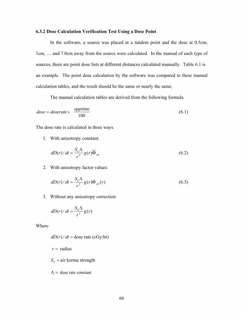
66
6.3.2 Dose Calculation Verification Test Using a Dose Point
In the software, a source was placed at a tandem point and the dose at 0.5cm,
1cm, … and 7.0cm away from the source were calculated. In the manual of each type of
sources, there are point dose lists at different distances calculated manually. Table 6.1 is
an example. The point dose calculation by the software was compared to these manual
calculation tables, and the result should be the same or nearly the same.
The manual calculation tables are derived from the following formula.
×= doseratedose100
apptime (6.1)
The dose rate is calculated in three ways.
1. With anisotropy constant:
ank rgr
SdtrdD Φ
Λ= )(/)( 2 (6.2)
2. With anisotropy factor values:
)()(/)( 2 rrgr
SdtrdD an
k ΦΛ
= (6.3)
3. Without any anisotropy correction
)(/)( 2 rgr
SdtrdD k Λ
=
Where
=dtrdD /)( dose rate (cGy/hr)
=r radius
=kS air kerma strength
=Λ dose rate constant

67
Table 6.1 Hand Calculation of Total Dose (Gy) for a 100 U 1–125 (STM1251) NIST 1999 Source Distance in (cm) Anisotropy constant Anisotropy
Factors No Anisotropy
Correction 0.50 7822.33 7830.64 8312.78 1.00 1893.11 1895.12 2011.81 1.50 788.38 787.12 837.81 2.00 405.13 403.40 430.53 2.50 233.84 234.09 248.50 3.00 145.35 146.28 154.46 3.50 94.58 94.88 100.51 4.00 63.89 63.89 67.90 4.50 44.41 44.34 47.19 5.00 31.43 31.33 33.40 5.50 22.81 22.77 24.24 6.00 16.51 16.51 17.55 6.50 12.32 12.34 13.09 7.00 9.12 9.15 9.69

68
=)(rg radial dose function
=Φan anisotropy constant
=Φ )(ran anisotropy factor
For permanent implants, the application time is calculated by:
(application time) = 1.44*24 hours/day * half-life
All distances are in centimeters. The half-life values are measured in days.
6.3.3 Dose Calculation Verification Test Using Isodose Contours
This test utilizes isodose contours to verify dose calculation. At the same time, it
also tests the proper isodose contour plot.
A source was put in the 1st image of an 11 image series, and these images are
0.5cm away from each other. Manually, doses at 0.5, 1.00 … 4.5cm away from a point
dose have been calculated (See example in table 6.2). The calculation formula are
equation 6.1 and 6.2.
Table 6.2 Nine calculated isodose levels for Pd-103 (1031L) [NIST 1999] source Distance
(cm) 0.5 1.00 1.50 2.00 2.50 3.00 3.50 4.00 4.50
Anisotropy Constant
1772.07 364.92 126.02 53.74 25.87 13.26 7.33 4.11 2.41
These doses were added as the isodose lines dose level to the software. If the
planning system calculation is correct, all nine isodose contours should be visible on
image #1. Each successive image should show one less isodose contour so that image #9
has only one contour left from the lowest isodose level. Also, the distance from the seed
to each contour should be within +/-2 mm of the expected value (0.5cm, 1.0cm …
4.5cm).

69
6.3.4 DVH and CVA Results Test
This test is used to verify the accuracy of VariSeed DVH (Dose Volume
Histogram) and CVA (Contiguous Volume Analysis) calculations and plotting.
A point dose was placed in the center of a series of images. The dose volume
with 10Gy (Pd-103) and 100Gy (I-125) had been manually calculated by equation 6.4
and 6.5.
V = 4/3*πr3 (6.4)
V = 1/3 δ*]*[ 11
2
0++
−
=
++∑ iii
N
ipApApA (6.5)
Equation 6.5 is the way VariSeed 6.7 calculates the dose volume. The expression
pA represents the area of the structure on an individual slice or scan; i indicates the scan
or slice position (first, second, etc.); t is the slice thickness; N is the number of slices
(scans). Table 6.3 is an example of dose volume calculation. The VariSeed application
uses a discrete representation of the dose, which causes the value of ipA to deviate
slightly from that of a perfect circle. Thus, the values displayed in this column are
different slightly from the values calculated by 4/3*πr3. Our test results are expected to
be close to the dose volume calculated by equation 6.5.
Table 6.3 DVH and CVA results test data for the I-125 (MED3631-A/S) [NIST 99] source
Activity U for: Dose Volume in cc for a Sphere of Radius r Using:
Radius in cm Anisotropy
Constant Anisotropy
Factor 4/3*πr3 Equation 6.5
1.0 5.204 5.293 4.19 3.52 1.5 12.605 13.100 14.14 13.04 2.0 24.549 26.085 33.51 31.96 2.5 42.686 43.336 65.45 63.43 3.0 69.288 67.343 113.10 110.59

70
6.4 Result
6.4.1 Reference Treatment Plan Comparison
6.4.1.1 Dose Information
Dose information comparison is the most quantitative way for the treatment plan
comparison. In the plan printout, it gives us the dose volume table and the volume dose
table. Table 6.4 and 6.5 are the comparisons between the reference plan and the QA plan.
Table 6.4 Prostate dose volume comparisons Reference plan QA Plan_1
(cc) Abs Volume Per Volume Abs Volume Per Volume Total Volume 18.53 N/A 18.38 N/A
V200 2.91 15.71% 2.82 15.33% V150 8.88 47.92% 8.82 47.97% V100 17.52 94.57% 17.37 94.51% V90 18.04 97.38% 17.93 97.58% V80 18.30 98.73% 18.15 98.74% V50 18.53 100% 18.38 100%
Table 6.5 Prostate volume dose comparison
Reference case Plan 1 Abs Dose (Gy) Per Dose Abs Dose (Gy) Per Dose
D100 72.24 50.51% 73.24 50.51% D90 155.67 107.36% 156.26 107.77% D80 173.48 119.64% 174.32 120.22% D50 215.25 148.45% 215.52 148.64%
It is very clear from the tables above that the QA plan is very well in accordance
with the reference plan.
6.4.1.2 Isodose Line Comparison
Because there are registration points on the images, it is easy to compare the
position of these lines between the reference plan and the QA plan. The comparison
between the QA plan and reference plan show very good consistence.

71
6.4.2 VariSeed Internal Test Procedure
There are altogether four types of seeds we are using at MBPCC. They are.
• I-125 (MED3631-A/M) NIST 1999
• Pd-103 (MED 3633) NIST 2000
• I-125 (STM1251) NIST 1999
• Pd-103 (1031L) [NIST 1999]
All of these four types of seeds were tested.
6.4.2.1 Dose Calculation Verification Test Using a Dose Point
The result is summarized as table 6.6.
6.4.2.2 Dose Calculation Verification Test Using Isodose Contours
The results (Figure 6.1) show that the number of isodose lines is reduced by one
from image#1 to image #9 as expected.
6.4.2.3 DVH and CVA Test Result
Table 6.7 (a,b,c,d) are the test results for the four types of seeds respectively.
From the DVH and CVA tests, 4 results were found off from the manual calculation by
more than 5% and they are highlighted inside the tables. Two of them are very close to
the calculated result of equation 6.4 and the differences to the equation 6.5 are also only a
little bit beyond 5% tolerance. The other two differences were significantly higher,
indicating the software has a miscalculation in these two cases.
6.5 Discussion
In the reference plan, the 100% and 150% isodose curves may not cover the
“tumor” well. But it really does not matter because we do not care about the treatment
result. As long as the reproducibility is verified, it is good enough for the QA purpose.

72
Table 6.6 Dose Calculation Verification Test Result Summaries a. I-125 (MED3631-A/M) NIST 1999 Anisotropy Constant Anisotropy Factor No Anisotropy Correction
Distance in (cm)
Manual Calculate
Test Result
Diff Manual Calculate
Test Result
Diff Manual Calculate
Test Result
Diff
0.5 8177.82 8177.8 0.02 8041.52 8041.5 0.02 9086.47 9086.5 0.031.00 1921.48 1921.5 0.02 9930.98 9931.0 0.02 11221.45 11221.4 0.051.50 793.36 793.4 0.04 10694.37 10694.4 0.03 12102.96 12103.0 0.042.00 407.35 467.4 0.05 11077.74 11077.7 0.04 12555.58 12555.6 0.022.50 234.27 234.3 0.03 11308.49 11308.5 0.01 12815.88 12815.9 0.023.00 144.32 144.3 0.02 11456.98 11457.0 0.02 12976.24 12976.2 0.043.50 93.49 93.5 0.01 11549.38 11549.4 0.02 13080.11 13080.1 0.014.00 62.81 62.8 0.01 11608.91 11608.9 0.01 13149.90 13149.9 0.004.50 43.46 43.5 0.04 11652.10 11652.1 0.00 13198.19 13198.2 0.015.00 30.82 30.8 0.02 11684.15 11684.2 0.05 13232.44 13232.4 0.045.50 22.61 22.6 0.01 11707.89 11707.9 0.01 13257.57 13257.5 0.076.00 16.60 16.6 0.00 11725.49 11725.5 0.01 13276.01 13276.0 0.01
b. Pd-103 (Med 3633) NIST 2000 Anisotropy Constant Anisotropy Factor No Anisotropy
Correction Distance in (cm)
Manual Calculate
Test Result
Diff Manual Calculate
Test Result
Diff Manual Calculate
Test Result
Diff
0.5 2015.48 2015.5 0.02 2062.51 2062.5 0.01 2239.43 2239.4 0.031.00 2406.08 2406.1 0.02 2462.22 2462.2 0.02 434.00 434.0 0.001.50 2538.88 2538.9 0.02 2595.76 2595.8 0.04 147.56 147.6 0.042.00 2595.13 2595.1 0.03 2651.32 2651.3 0.02 62.50 62.5 0.002.50 2621.69 2621.7 0.01 2676.54 2676.5 0.04 29.51 29.5 0.013.00 2635.14 2635.1 0.04 2688.8 2688.8 0.00 14.95 14.9 0.053.50 2642.28 2642.3 0.02 2695.36 2695.4 0.04 7.94 7.9 0.044.00 2646.31 2646.3 0.01 2699.09 2699.1 0.01 4.48 4.5 0.024.50 2648.68 2648.7 0.02 2701.36 2701.4 0.04 2.64 2.6 0.045.00 2650.08 2650.1 0.02 2702.74 2702.7 0.04 1.55 1.6 0.055.50 2650.89 2650.9 0.01 2703.54 2703.5 0.04 0.90 0.9 0.006.00 2651.39 2651.4 0.01 2704.03 2704.0 0.03 0.55 0.6 0.05
(Table cont’d)

73
d. 103 (1031L) NIST 1999 Anisotropy Constant Anisotropy Factor No Anisotropy Correction
Distance in (cm)
Manual Calculate
Test Result
Diff Manual Calculate
Test Result
Diff Manual Calculate
Test Result
Diff
0.5 1772.07 1772.1 0.03 1795.86 1795.9 0.04 1982.18 1982.2 0.02 1.00 364.92 364.9 0.02 367.78 367.8 0.02 408.19 408.2 0.01 1.50 126.02 126.0 0.02 126.30 126.3 0.00 140.96 141.0 0.04 2.00 53.74 53.7 0.04 53.55 53.6 0.05 60.11 60.1 0.01 2.50 25.87 25.9 0.03 25.75 25.8 0.05 28.93 28.9 0.03 3.00 13.26 13.3 0.04 13.18 13.2 0.02 14.83 14.8 0.03 3.50 7.33 7.3 0.03 7.29 7.3 0.01 8.20 8.2 0.00 4.00 4.11 4.1 0.01 4.09 4.1 0.01 4.59 4.6 0.01 4.50 2.41 2.4 0.01 2.41 2.4 0.01 2.70 2.7 0.00 5.00 1.43 1.4 0.03 1.43 1.4 0.03 1.60 1.6 0.00 5.50 0.92 0.9 0.02 0.91 0.9 0.01 1.03 1.0 0.03 6.00 0.54 0.5 0.04 0.54 0.5 0.04 0.60 0.6 0.00
c. I-125 (STM1251) NIST 1999 Anisotropy Constant Anisotropy Factor No Anisotropy Correction
Distance in (cm)
Manual Calculate
Test Result
Diff Manual Calculate
Test Result
Diff Manual Calculate
Test Result
Diff
0.5 7822.33 7822.3 0.03 7830.64 7830.6 0.04 8312.78 8312.8 0.021.00 9715.44 9715.4 0.04 1895.12 1895.1 0.02 10324.59 10324.6 0.011.50 10503.82 10503.8 0.02 787.12 787.1 0.02 11162.40 11162.4 0.002.00 10908.95 10908.9 0.05 403.40 403.4 0.00 11592.93 11592.9 0.032.50 11142.79 11142.8 0.01 234.09 234.1 0.01 11841.43 11841.4 0.033.00 11288.14 11288.1 0.04 146.28 146.3 0.02 11995.89 11995.9 0.013.50 11382.72 11382.7 0.02 94.88 94.9 0.02 12096.40 12096.4 0.004.00 11446.61 11446.6 0.01 63.89 63.9 0.01 12144.30 12164.3 0.004.50 11491.02 11491.0 0.02 44.34 44.3 0.04 12211.49 12211.5 0.015.00 11522.45 11522.4 0.05 31.33 31.3 0.03 12244.89 12244.9 0.015.50 11545.26 11545.2 0.06 22.77 22.8 0.03 12269.13 12269.1 0.036.00 11561.77 11561.8 0.03 16.51 16.5 0.01 12286.68 12286.7 0.02

74
Figure 6.1 Dose calculation verification result using isodose lines

75
Table 6.7 DVH and CVA Test Result Summary a. I-125 (MED3631-A/M) NIST 1999
Radius in cm 4/3*πr3 Equation 6.5 Constant Difference Factor Difference1.0 4.19 3.52 3.51 -0.28% 3.54 +0.57% 1.5 14.14 13.04 13.07 -0.23% 13.07 +0.23% 2.0 33.51 31.96 32.01 -0.16% 32.01 +0.16% 2.5 65.45 63.43 63.38 +0.08% 62.38 -1.66% 3.0 113.10 110.59 110.57 +0.02% 110.63 +0.04%
b. Pd-103 (Med 3633) NIST 2000
Radius in cm 4/3*πr3 Equation 6.5 Constant Difference Factor Difference1.0 4.19 3.52 3.51 -0.30% 3.46 +1.7% 1.5 14.14 13.04 13.19 +1.1% 12.85 +1.5% 2.0 33.51 31.96 32.32 +1.1% 31.37 +1.8% 2.5 65.45 63.43 64.52 +1.7% 67.67 -0.38% 3.0 113.10 110.59 113.34 +0.25% 124.32 -12.4%
c. I-125 (STM1251) NIST 1999
Radius in cm 4/3*πr3 Equation 6.5 Constant Difference Factor Difference1.0 4.19 3.52 3.51 +0.28% 3.54 +0.56% 1.5 14.14 13.04 13.03 +0.08% 13.07 +0.23% 2.0 33.51 31.96 32.01 -0.16% 31.95 -0.03% 2.5 65.45 63.43 63.44 -0.02% 63.38 -0.08% 3.0 113.10 110.59 110.57 +0.02% 110.57 -0.02%
d. Pd-103 (1031L) NIST 1999
Radius in cm 4/3*πr3 Equation 6.5 Constant Difference Factor Difference1.0 4.19 3.52 3.63 +3.1% 4.12 -17.0% 1.5 14.14 13.04 13.13 +0.69% 13.72 -5.21% 2.0 33.51 31.96 31.85 -0.35% 32.57 -1.91% 2.5 65.45 63.43 63.13 -0.57% 65.80 -3.74% 3.0 113.10 110.59 110.14 -0.41% 116.96 -5.76%

76
6.6 Conclusion
The VariSeed 6.7 prostate treatment planning system accuracy can be verified by
the reference plan comparison with reliability. The dose calculation verification test,
dose calculation verification test using isodose contours, DVH and CVA results test are
good supplements to the QA procedures.

77
CHAPTER 7. PLATO-BRACHYTHERAPY TPS QA
7.1 Introduction
PLATO-Brachytherapy TPS is used as an HDR planning system at MBPCC. It
runs on Indigo and Indy workstations under the Silicon Graphics IRIX operating system,
a Silicon Graphics implementation of UNIX. PLATO-TPS can be used to make standard
and non-standard treatment plans for microSelectron-HDR, microSelectron-PDR,
Selectron-LDR/MDR and Selectron-HDR afterloaders.
Stam (1998) did commissioning and evaluation of the PLATO-
BRACHYTHERAPY TPS about 5 years ago. But after that, none of the TPS QA has
been performed.
Dose distribution calculation in PLATO is based on point dose calculations. The
calculation of an absorbed dose to a particular point begins at the level of the exposure
rate distribution of a source. Then it is converted to dose by f factor, which is called the
roentgen to rad conversion factor. After the attenuation and scatter correction, the total
dose to a particular point is calculated by summing the contribution to a point from each
dwell position of the source. The calculation formula can be written as:
Total ∑=
×××Γ×=n
ipipip TdMFAradD
1
2 )/()()( (7.1)
Where A is the activity of source (Ci),
Γ is gamma factor or exposure rate constant (R×cm2/Ci-sec),
T is time of exposure or dwell time (sec), d is distance from the source,
F is f factor,
M is Meisberger factor,

78
n is the total number of dwell positions,
i denotes one dwell position.
The isotope used in MBPCC HDR system is Ir-192. It has a low average gamma
ray energy of 0.38 MeV and a small half value layer (2.5 mm of lead). Its half-life is
74.02 days, which makes it necessary to be replaced every four months.
7.2 Methodology
7.2.1 Reference Case
The basic idea of PLATO Brachytherapy Computer QA is still the same as
Pinnacle3 QA. It mainly tests the reproducibility of the system. Initially, two reference
treatment plans were established. Whenever the source is changed or the treatment
planning result is doubtful, the reference plans can be repeated, and the result is
compared to the reference plan.
7.2.1.1 Reference Plan Making
One of the reference cases is vagina cylinder treatment planning. The reference
dose points are 5mm away from the outside of the cylinder.
The other reference case is tandem and ring treatment planning. There are four
films (AP, Lateral, LAO and RAO) in this case. In order to be able to repeat the plan, all
the points and catheter positions were plotted on a graph paper with the same relative
positions.
7.2.1.2 QA Plan Making
In QA plan making, the exact same treatment planning procedures were executed
as in the reference plan. It includes the same films, the same catheter positions, the same
source positions, the same prescription and the same optimization method. If the

79
treatment planning system has been working consistently, the only difference between the
QA plan and reference plan would be the source decay factor or the source strength ratio.
In addition, three 2-D plots (AP, lateral and transversal) were printed out with
isodose lines. Because these isodose lines are in the form of percentage, the plot should
be exactly the same each time.
7.2.2 Software Calculation Test
Sometimes, the reference tests may show a difference beyond the tolerance for
some reason. It is probably because the catheter points and the reference points can’t be
digitized perfectly in the same position each time. But in order to verify if it is the true
reason, the software calculation test is necessary. This test does not include the step of
digitizing the image. Instead, it clears the source position, prescription, optimization
method, and dose calculation in the reference plan first. Following that, the same
prescription, optimization method and dose calculation were added up or executed again.
This test is not affected by the digitizer, so the tolerance recommended is more strictly at
1%.
7.2.3 Digitizer Test
Since all of the Plato HDR treatment planning inputs are from the digitizer, QA
for the digitizer is much more important compared to the Pinnacle3 digitizer QA. Also
because the digitizer is the most easily broken part of the PLATO planning system, it is
tested monthly or quarterly depending on the number of HDR cases. The test procedure
is the same as the Pinnacle3 digitizer test.

80
7.2.4 Checksum Test
Because Plato HDR TPS software is also installed in a Unix system, a checksum
program can also be utilized. The spot checking file signatures can further ensure the
consistency of the software.
7.2.5 Output Check
For the HDR machine, monthly QA was set up to check the source position and
source strength. Also, every morning before the HDR procedure, a preplan QA is
performed to check the working condition of the machine, such as source position
verification, console interrupt, measured dwell time, etc.
7.2.5 Verification Frequency
Since there are not many HDR cases at MBPCC, the QA test can be performed
every six months or whenever the source is replaced. If it is for the later reason, our test
doubly checks the accuracy of the new source strength input.
7.3 Result and Analyses
7.3.1 Tandem & Ring Case
7.3.1.1 Dose Information
Table 7.1 is the list of source time, dose on catheters and decay factor. Initial
dose rate was used for comparison and it was calculated by:
Initial dose rate = Dose / (Absolute time x DF) x ( newsourceoldsource AA / ) (7.1)
Where oldsourceA is initial activity of the old source and
newsourceA is initial activity of the new source.
Initial dose rate should have the same value if the PLATO TPS is working
consistently.

81
Table 7.1 Initial dose rate comparison in Tandem & Ring case Abs time (sec) Dose Decay factor Initial dose rate
Point Ref QA Ref QA Ref QA Ref QA Tandem 26.7 24.6 41.43 41.70
Ring 44.5 41.0 568.53 569.35 0.514 0.555
24.86 25.02 7.3.1.2 Point Coordinates
The point coordinate comparison is illustrated in table 7.2.
Table 7.2 Point Coordinate comparisons in Tandem & Ring case Point X (mm) Y (mm) Z (mm) Dose (cGy)
Ref Plan 6.3 64.4 22.7 83.72 QA Plan 6.9 64.1 22.6 84.12
Bladder
Diff +9.5% -0.5% -0.4% +0.5% Ref Plan 37.2 78.5 56.5 41.23 QA Plan 37.5 78.4 56.6 41.02
Rectum
Diff +0.8% -0.1% +0.2% -0.5%
From the table above, it is found that the X coordinate of the bladder point is off
by +9.5%. But the absolute value difference is only 0.3mm, which can be negligible.
7.3.2 Vagina Cylinder Case
7.3.2.1 Dose Information
In this case, the prescription dose is on the dose points with 17.5mm away from
the catheter. The point doses were compared first (Table 7.3), and then the treatment
time calculation was checked (Table 7.4 and figure 7.1).
From the comparison, it can be seen that most of the results are good to be within
the tolerance except 5 absolute time comparisons in the Vagina Cylinder case. However,
the total treatment time comparison was the same. In order to ensure the error is because
the catheter points in the reference case and the QA plan were not digitized in the same
exact point, the software calculation test was performed, and the comparison result is in
table 7.6.

82
Table 7.3 Point dose comparison in Vagina Cylinder case Dose
Point Ref QA Difference 1 445.90 443.24 -0.60% 2 499.89 501.06 +0.23% 3 521.24 528.87 +1.46% 4 524.65 523.29 -0.26% 5 518.54 506.19 -2.38% 6 500.00 498.10 +0.38% 7 485.67 497.89 +2.51% 8 495.13 498.31 +0.64% 9 511.85 507.02 -0.94% 10 524.51 523.37 -0.22% 11 524.62 527.65 +0.58% 12 501.94 501.16 -0.16% 13 445.76 443.84 -0.43%
Table 7.4 Absolute time comparison after correction by decay factor
Abs time (sec) Decay factor Time after DF correction Point Ref QA Ref QA Ref QA Difference
1 69.1 67.9 0.514 0.490 35.517 33.271 -6.3% 2 60.9 60.3 0.514 0.490 31.303 29.547 -5.6% 3 48.0 48.7 0.514 0.490 24.672 23.863 -3.3% 4 35.3 37.4 0.514 0.490 18.144 18.326 +1.0% 5 26.3 29.0 0.514 0.490 13.518 14.21 +5.1% 6 21.7 24.5 0.514 0.490 11.154 12.005 +7.6% 7 20.9 23.2 0.514 0.490 10.743 11.368 +5.8% 8 22.9 24.6 0.514 0.490 11.771 12.054 +2.4% 9 28.0 29.3 0.514 0.490 14.392 14.357 -0.2% 10 36.8 37.9 0.514 0.490 18.915 18.571 -1.8% 11 48.8 49.7 0.514 0.490 25.083 24.353 -2.9% 12 61.1 61.8 0.514 0.490 31.405 30.282 -3.6% 13 69.0 69.6 0.514 0.490 35.466 34.104 -3.8%
Total 548.8 563.9 0.514 0.490 282.08 276.31 -2.0%

83
Absolute time comparison after correction of Decay Factor
Piont
0 2 4 6 8 10 12 14
Abs
olut
e tim
e af
ter c
orre
ctio
n of
dec
ay fa
ctor
5
10
15
20
25
30
35
40
Reference PlanQA Plan
Figure 7.1 Absolute time comparisons
after correction of decay factor in Vagina Cylinder case

84
7.3.2.2 Point Coordinate
Table 7.5 Point coordinate comparison in Vagina Cylinder case Point Plan X (mm) Y (mm) Z (mm) Dose (cGy)
Ref Plan 20.8 19.2 -10.1 222.15 QA Plan 20.8 19.8 -10.1 213.27
Pt 1
Diff 0.0% +3.1% 0.0% -4.0% Ref Plan -19.0 -20.8 20.1 268.28 QA Plan -19.3 -20.6 20.0 266.27
Pt 2
Diff -1.6% +1.0% +0.5% +0.8% Table 7.6 Point dose comparison in software calculation test
Abs time (sec) Decay factor Time after DF correction Point Ref QA Ref QA Ref QA Difference
1 69.1 91.2 0.514 0.389 35.517 35.477 -0.11% 2 60.9 80.3 0.514 0.389 31.303 31.237 -0.21% 3 48.0 63.3 0.514 0.389 24.672 24.624 -0.20% 4 35.3 46.6 0.514 0.389 18.144 18.127 -0.09% 5 26.3 34.7 0.514 0.389 13.518 13.498 -0.15% 6 21.7 28.7 0.514 0.389 11.154 11.164 +0.09% 7 20.9 27.5 0.514 0.389 10.743 10.698 -0.42% 8 22.9 30.2 0.514 0.389 11.771 11.748 -0.20% 9 28.0 36.9 0.514 0.389 14.392 14.354 -0.26% 10 36.8 48.6 0.514 0.389 18.915 18.905 -0.05% 11 48.8 64.4 0.514 0.389 25.083 25.052 -0.13% 12 61.1 80.6 0.514 0.389 31.405 31.353 -0.16% 13 69.0 91.0 0.514 0.389 35.466 35.466 -0.19%
Total 548.8 724.0 0.514 0.389 282.08 282.08 -0.16% The result shows the software calculation is still correct. The difference out of
tolerance between the QA plan and the reference plan must have been caused by
digitization.
7.3.3 Digitizer Test
Three squares (twelve points) were tested. The result is demonstrated in table 7.7
and it shows the digitizer is in good working conditions.
7.4 Discussion
The HDR treatment program data is transferred to the HDR machine by a
program card. Although our QA procedures check the treatment planning software and
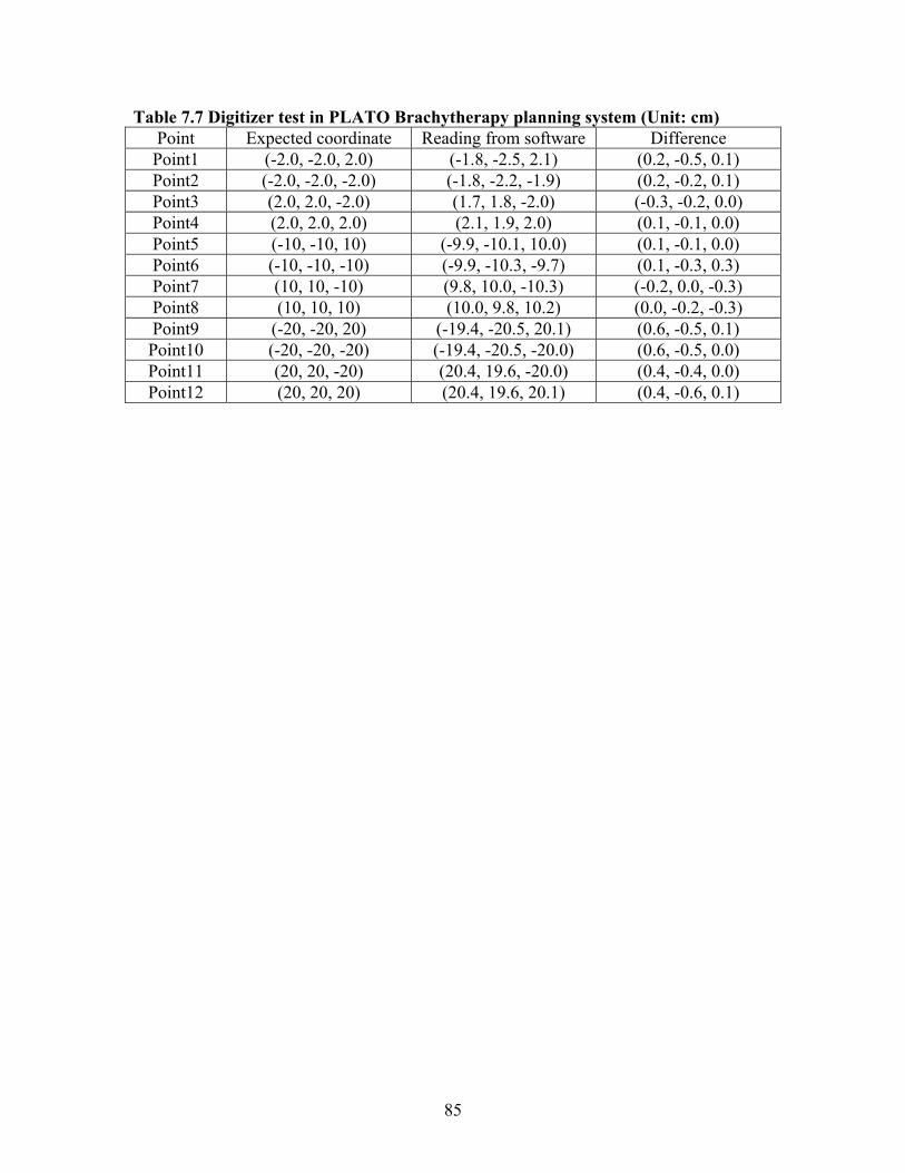
85
Table 7.7 Digitizer test in PLATO Brachytherapy planning system (Unit: cm) Point Expected coordinate Reading from software Difference Point1 (-2.0, -2.0, 2.0) (-1.8, -2.5, 2.1) (0.2, -0.5, 0.1) Point2 (-2.0, -2.0, -2.0) (-1.8, -2.2, -1.9) (0.2, -0.2, 0.1) Point3 (2.0, 2.0, -2.0) (1.7, 1.8, -2.0) (-0.3, -0.2, 0.0) Point4 (2.0, 2.0, 2.0) (2.1, 1.9, 2.0) (0.1, -0.1, 0.0) Point5 (-10, -10, 10) (-9.9, -10.1, 10.0) (0.1, -0.1, 0.0) Point6 (-10, -10, -10) (-9.9, -10.3, -9.7) (0.1, -0.3, 0.3) Point7 (10, 10, -10) (9.8, 10.0, -10.3) (-0.2, 0.0, -0.3) Point8 (10, 10, 10) (10.0, 9.8, 10.2) (0.0, -0.2, -0.3) Point9 (-20, -20, 20) (-19.4, -20.5, 20.1) (0.6, -0.5, 0.1) Point10 (-20, -20, -20) (-19.4, -20.5, -20.0) (0.6, -0.5, 0.0) Point11 (20, 20, -20) (20.4, 19.6, -20.0) (0.4, -0.4, 0.0) Point12 (20, 20, 20) (20.4, 19.6, 20.1) (0.4, -0.6, 0.1)

86
HDR machine separately, no data transfer accuracy can be verified. It would be of
significance if a simple treatment program can be made in the software and sent to a
program card. Then run the plan on the HDR machine and test the source position and
strength. However, this procedure would take much more time.
7.5 Conclusion
By the reference plan comparison and frequent digitizer test, the PLATO HDR
treatment planning system was efficiently checked. The total test time is less than half an
hour. Until now, no significant error has been found and it is safe to say that the system
is working with consistency.

87
CHAPTER 8. GLOBAL DISCUSSION
8.1 Test of Whole Radiation Treatment Process
In chapter 4, the integration of CT and Pinnacle3 was verified. However, that is
only a partition of the whole radiation treatment process. It would be valuable if the QA
test would start from CT and end up with the LINACS.
A test was performed to test an IMRT plan on a 21EX(BR) machine. A RANDO
phantom was utilized to simulate the patient’s head and scanned in the CT-Simulator.
Then an IMRT plan was transferred to the phantom images. Some KODAK XV-2 films
were sandwiched between RANDO phantom slices and the phantom was treated in
21EX(BR) (Figure 8.1). Finally those films were analyzed in RIT 113 software (RIT,
Inc) and the measured dose profiles were compared to the ADAC calculation.
There are two advantages that make this test better than the regular IMRT QA
used currently at MBPCC.
First, the RANDO phantom is inhomogeneous, which allows the actual dose
distribution in heterogeneous materials to be checked. The regular IMRT QA procedure
at MBPCC utilizes two 30cm X 30cm X 10cm solid water phantoms. It is always
doubtful if the homogeneous dose calculation would fit the measurement as well in an
inhomogeneous patient’s body.
Secondly, this test starts from the CT-simulator, and simulates the entire patient
treatment process. Any systematic error would be caught easily. For example, the
RANDO phantom was moved from the CT scan location (B. B. marker aligns with the
CT laser) to the LINACS position (B. B. marker align with the LINACS laser) and then
changed to treatment position (Isocenter) according to the ADAC treatment plan report.

88
The CT laser and LINACS laser system may be easily checked independently, but their
relative position could be off. Our test can find out this kind of error.
Figure 8.1 RANDO phantom in treatment room The result is shown in figure 8.2.
From the profiles comparison, it is easy to see that the results are good overall.
However, in most central areas, the measurement does not fit for the calculation within
the tolerance. In our experiment, there are still two aspects that could be changed to
improve the accuracy. First, there are thousands of holes inside the RANDO phantom.
This special geometry makes both the Pinnacle3 calculation and film measurement much
more complicated. Filling out these holes with plugs could definitely improve the
measurement accuracy. Another way is to let the RANDO phantom slices lie on each
other when it is scanned and treated. By this way, there won’t be an air crevice between
the phantom slices, which affects the measurement, when the film is sandwiched in.
8.2 Test from Treatment Planning Computers to the LINACS
The regular IMRT QA procedure at MBPCC does check the accuracy from treatment
planning computers to the LINACS. However, IMRT can only be implemented in the

89
(a) LSObrain dose profile (vertical) (b) LSObrain dose profile (Perpendicular) (c) Vertex dose profile (Perpendicular) (d) Vertex dose profile (Vertical) (e) RSO dose profile (Perpendicular) (f) RSO dose profile (Vertical)
(g) Composite dose profile (Perpendicular) (h) Composite dose profile (Vertical) Figure 8.2 Test result of whole treatment process. (The dotted line and solid line are
calculation and measurement respectively)

90
21EX(BR) and 21EX(COV). A similar way can be used for 2100C, 2000CR(Ham) and
600C. Instead of shooting an IMRT plan on the KODAK XV-2 film, a 3-D conformal
treatment plan was imposed on the film. This plan includes wedges and blocks. The
other procedures are the same as a regular IMRT plan: the dose distribution in a plane
was achieved from ADAC; shoot film sandwiched between solid water blocks; and
analyze them by RIT software.
In this test, the dose accuracy, dose distribution symmetry, wedge factor, tray
factor, the position of blocks in the mount and a lot of other characters can be verified at
the same time. Our result is shown in figure 8.3.
The result shows measurements and calculations fit better to each other in
PA_boost field. But in right boost field, the difference is as large as 10%.
One of the problems in the experiment above is that the film analysis has a pretty
high uncertainty compared to other dosimetry tools. A better way is to put a TLD inside
the RANDO phantom holes or use the gel dosimetry to measure the dose distribution
directly. But these two methods are too expensive to be used in a clinic.

91
(a) PA_boost dose profile (Vertical) (b) PA_boost dose profile (Perpendicular) (c) RT_boost dose profile (Vertical) (d) RT_boost dose profile (Perpendicular)
Figure 8.3 Test result from treatment planning computers to the LINACS (The dotted line and solid line are calculation and measurement respectively)

92
CHAPTER 9. GLOBAL CONCLUSION
QA procedures for all of the treatment planning systems at MBPCC were
established based on the idea of simulating the actual patient treatment process. They are
fast and effective, but not perfect. There are still many other QA tests that could be
performed, and much more characteristics of the TPS could be checked. However, it
would make the whole TPS QA too time consuming and inefficient for clinical use. It
should be understood that all possible sources of error can never be tested.
In the experiment from July to September, our test results show all of the
treatment planning systems at MBPCC worked well. Although no large errors have been
found yet, the QA should not be taken for granted. Quality assurance for treatment
planning systems is a very extensive process. It is an evolving subject that keeps
changing with improvements in treatment planning computers. MBPCC medical
physicists should review the latest development and keep up with improvements in QA
testing.

93
REFERENCES
1. Fraass B. Doppke K, Hunt M, Kutcher G, Starkschall G, Stern R, Van Dyke J. AAPM Radiation Therapy Committee Task Group 53: quality assurance fro clinical radiotherapy treatment planning. Med. Phys. 1998; 25: 1773-1829.
2. G. Kutcher et al., “Comprehensive QA for radiation oncology: Report of AAPM
Radiation Therapy Committee Task Group 40,” Med. Phys. 21, 581-618 (1994).
3. Ten Haken, R.K., Fraass, B.A. (1996). Quality assurance in 3D treatment planning. Front. Radiat. Ther. Oncol. 29: 104-114
4. Frass, B.A (1996). Quality assurance for 3-D treatment planning. In: Mackie,
T.R., Palta J.R., eds. Teletherapy: Present and Future. Madison WI: Advanced Medical Publishing: 253-318.
5. Dahlin, H.; Lamm, I. L.; Landberg, T.; Levernes, S.; Ulso, N. User requirements
on CT based computerized dose planning systems in radiotherapy. Acta Radiol. Oncol. 22: 398-415; 1983.
6. Bruce Curran, George Starkschall: “A program for quality assurance of dose
planning computers”, in Quality Assurance in Radiotherapy Physics, proceedings of an American College of Medical Physics Symposium edited by George Starkschall and John Horton (Medical Physics Publishing, Madison, WI 1991), pp 207-228.
7. ICRU: ICRU Report 29, “Dose specification for reporting external beam therapy
with photons and electrons,” Bethesda, MD, International Committee on Radiation Units and Measurements, 1978.
8. George Starkschall, Roy E. Steadham, Jr., Richard A. Popple, Salahuddin Ahmad,
and Isaac I. Rosen: Beam-commissioning methodology for a three dimensional convolution/superposition photon dose algorithm. Journal of Applied Clinical Medical Physics, 2000, 1; 8-27.
9. J. Van Dyk, R. Barnett, J. Cygler, and P. Shragg, (1993) “Commissioning and
quality assurance of treatment planning computers,” Int. J. Radiat. Oncol., Biol., Phys. 26, 261-273.
10. T. R. Mackie, J. W. Scrimger, and K. K. Battista, “ A convolution method of
calculation dose for 15-MV x-rays,” Med. Phys. 12, 188-196 (1985).
11. An ADAC Pinnacle3 Physics Guide, ADAC Laboratories, Milpitas, California, 2001.

94
12. AAPM Report # 55, “Radiation Treatment Planning Dosimetry Verification, Radiation Therapy Committee Task Group #23,” edited by D. Miller (American Institute of Physics, College Park, MD, 1995).
13. Hogstrom, K. R, Millers, M.D., and Almond, P.R. 1981. Electron beam dose
calculations. Physics of Medicine and Biology 26: 445-459.
14. M. L. Kessler, R. K. Ten Haken, B. A. Frass, and D. L. McShan, “Expanding the use and effectiveness of dose-volume histograms for 3D treatment planning, I. Integration of 3-D dose-display,” Int. J. Radiat. Oncol., Biol., Phys. 29, 1125-1131 (1994).
15. R. Nath, L. L. Anderson, G. Luxton, K. A. Weaver, J. F. Williamson, and A. S.
Meigooni, “Dosimetry of interstitial brachytherapy sources: Recommendations of the AAPM Radiation Therapy Committee Task Group No. 43, “ Med. Phys. 22, 209-234 (1995).
16. K. P. McGee, and I. J. Das: Commissioning, Acceptance testing, & quality
assurance of a CT simulator (2000), Shirish Jani, eds, CT Simulation for Radiotherapy, Medical Physics Publishing: 5-23.
17. Nagata Y, Nishidai T. Abe M, Takahashi M, Yukawa, Nohara H, Yamaoka N,
Saida T, Ishihara H, Kubo Y, Ohta H, Inamura K. CT simulator: A new treatment planning system for radiotherapy. Int J Rad Oncol Biol Phys 1990; 13-176.
18. Nishidai T Nagato Y, Takahashi M, Abe M, Yamaoka N, Ishihara H, Kubo Y,
Ohta H, Kazusa C. CT simulator: a new 3-D planning and simulating system for radiotherapy: part I. Description of system. Int J Rad Oncol Biol Phys 1989; 18: 499-504.
19. Sherouse GW, Novins K, Chaney E. Computation of digitally reconstructed
radiography for use in radiotherapy treatment design. Int J Rad Oncol Biol Phys 1990; 18: 651-658.
20. Lawrence Rothenberg: Quality Control in CT, 2002 AAPM Annual Meeting.
21. A VariSeed User Guide for version 6.7, Varian Medical System, Inc, California,
2000.
22. A Nucletron Corporation User Manual. New Implementations for Version 10.11. Nucletron Corporation, Columbia, Maryland, 1995, pp. 4-7.
23. Angela Stam: Commissioning and evaluation of the PLATO-Brachytherapy
planning system. Master thesis, 1998.

95
24. Ravinder Nath, Lowell L. Anderson, Jerome A. Meli, Arthur J.Olch, Judith Anne Stitt, Jeffrey F. Williamson: AAPM Radiation Therapy Committee Task Group 56: Code of practice for brachytherapy physics. Med. Phys. 1997; 25: 1557-1598.

96
VITA
Junqing Wu was born in Guixi city of Jiangxi Province, People’s Republic of
China. He received a Bachelor of Science degree from Peking University in July 2000.
He began his graduate work in the Department of Physics and Astronomy in the Fall of
2000. Junqing will receive a Master of Science degree from the Department of Physics
and Astronomy at Louisiana State University in the Fall of 2002.