Ali A. AmeriThe Ohio State University, Columbus, Ohio

Implementation of a Transition Model in a NASA Code and Validation Using Heat Transfer Data ona Turbine Blade

NASA/CR—2012-217436

April 2012

https://ntrs.nasa.gov/search.jsp?R=20120009201 2018-05-20T03:45:50+00:00Z

NASA STI Program . . . in Profi le

Since its founding, NASA has been dedicated to the advancement of aeronautics and space science. The NASA Scientifi c and Technical Information (STI) program plays a key part in helping NASA maintain this important role.

The NASA STI Program operates under the auspices of the Agency Chief Information Offi cer. It collects, organizes, provides for archiving, and disseminates NASA’s STI. The NASA STI program provides access to the NASA Aeronautics and Space Database and its public interface, the NASA Technical Reports Server, thus providing one of the largest collections of aeronautical and space science STI in the world. Results are published in both non-NASA channels and by NASA in the NASA STI Report Series, which includes the following report types: • TECHNICAL PUBLICATION. Reports of

completed research or a major signifi cant phase of research that present the results of NASA programs and include extensive data or theoretical analysis. Includes compilations of signifi cant scientifi c and technical data and information deemed to be of continuing reference value. NASA counterpart of peer-reviewed formal professional papers but has less stringent limitations on manuscript length and extent of graphic presentations.

• TECHNICAL MEMORANDUM. Scientifi c

and technical fi ndings that are preliminary or of specialized interest, e.g., quick release reports, working papers, and bibliographies that contain minimal annotation. Does not contain extensive analysis.

• CONTRACTOR REPORT. Scientifi c and

technical fi ndings by NASA-sponsored contractors and grantees.

• CONFERENCE PUBLICATION. Collected papers from scientifi c and technical conferences, symposia, seminars, or other meetings sponsored or cosponsored by NASA.

• SPECIAL PUBLICATION. Scientifi c,

technical, or historical information from NASA programs, projects, and missions, often concerned with subjects having substantial public interest.

• TECHNICAL TRANSLATION. English-

language translations of foreign scientifi c and technical material pertinent to NASA’s mission.

Specialized services also include creating custom thesauri, building customized databases, organizing and publishing research results.

For more information about the NASA STI program, see the following:

• Access the NASA STI program home page at http://www.sti.nasa.gov

• E-mail your question via the Internet to help@

sti.nasa.gov • Fax your question to the NASA STI Help Desk

at 443–757–5803 • Telephone the NASA STI Help Desk at 443–757–5802 • Write to:

NASA Center for AeroSpace Information (CASI) 7115 Standard Drive Hanover, MD 21076–1320

Ali A. AmeriThe Ohio State University, Columbus, Ohio

Implementation of a Transition Model in a NASA Code and Validation Using Heat Transfer Data ona Turbine Blade

NASA/CR—2012-217436

April 2012

National Aeronautics andSpace Administration

Glenn Research CenterCleveland, Ohio 44135

Prepared under Contract NNC06BA07B, Task NNC10E420T-0

Available from

NASA Center for Aerospace Information7115 Standard DriveHanover, MD 21076–1320

National Technical Information Service5301 Shawnee Road

Alexandria, VA 22312

Available electronically at http://www.sti.nasa.gov

Trade names and trademarks are used in this report for identifi cation only. Their usage does not constitute an offi cial endorsement, either expressed or implied, by the National Aeronautics and

Space Administration.

This work was sponsored by the Fundamental Aeronautics Program at the NASA Glenn Research Center.

Level of Review: This material has been technically reviewed by NASA expert reviewer(s).

This report contains preliminary fi ndings, subject to revision as analysis proceeds.

NASA/CR—2012-217436 1

Implementation of a Transition Model in a NASA Code and Validation Using Heat Transfer Data on a Turbine Blade

Ali A. Ameri

The Ohio State University Columbus, Ohio 43210

Abstract

The purpose of this report is to summarize and document the work done to enable a NASA CFD code to model laminar-turbulent transition process on an isolated turbine blade. The ultimate purpose of the present work is to down-select a transition model that would allow the flow simulation of a variable speed power turbine to be accurately performed. The flow modeling in its final form will account for the blade row interactions and their effects on transition which would lead to accurate accounting for losses. The present work only concerns itself with steady flows of variable inlet turbulence. The low Reynolds number k- model of Wilcox and a modified version of the same model will be used for modeling of transition on experimentally measured blade pressure and heat transfer. It will be shown that the k- model and its modified variant fail to simulate the transition with any degree of accuracy. A case is thus made for the adoption of more accurate transition models. Three-equation models based on the work of Mayle on Laminar Kinetic Energy were explored. The three-equation model of Walters and Leylek was thought to be in a relatively mature state of development and was implemented in the Glenn-HT code. Two-dimensional heat transfer predictions of flat plate flow and two-dimensional and three-dimensional heat transfer predictions on a turbine blade were performed and reported herein. Surface heat transfer rate serves as sensitive indicator of transition. With the newly implemented model, it was shown that the simulation of transition process is much improved over the baseline k- model for the single Reynolds number and pressure ratio attempted; while agreement with heat transfer data became more satisfactory. Armed with the new transition model, total-pressure losses of computed three-dimensional flow of E3 tip section cascade were compared to the experimental data for a range of incidence angles. The results obtained, form a partial loss bucket for the chosen blade. In time the loss bucket will be populated with losses at additional incidences. Results obtained thus far will be discussed herein.

Nomenclature

Cp loss coefficient Cf friction coefficient Cx axial chord E turbulent energy spectral density h heat transfer coefficient k turbulence kinetic energy M Mach number Nu Nusselt number P pressure Pr Prandtl number q wall heat flux r recovery factor Re Reynolds number = ( U) Cx/ subscripts “1”, “2” and are defined below. St Stanton number = Nu/(Re*Pr)

NASA/CR—2012-217436 2

T temperature Tu turbulence intensity (u/ u) u flow velocity x axial distance y pitchwise coordinate z spanwise distance Subscripts: 0 total (stagnation) condition 1 conditions based on mass flow per unit area and inlet conditions 2 conditions based on isentropic exit condition aw adiabatic wall value eff effective eddy size used in Reference 5 in inlet condition l laminar condition T turbulent condition s static isentropic condition t total value w wall value x local value ∞ free stream condition fluctuating component Greek: γ specific heat ratio inlet boundary layer thickness cnditions based on local isentropic values and momentum thickness wave number associated with fluctuating eddies wave length specific turbulent dissipation dynamic viscosity fluid density specific turbulent dissipation

Introduction

A key goal of the Subsonic Rotary Wing project is to enhance utilization of civil rotorcraft to relieve airport congestion and increase throughput capacity. One concept that has been advocated for this purpose is the use of tilt rotors to enable vertical takeoff and landing. In order to bring about fuel efficiency the main-rotor speed varies from 100 percent at takeoff to 50 percent at cruise. This can be achieved by using a two-speed transmission driven by a power turbine with minimal speed change. To avoid the added weight of the two-speed transmission a variable speed power turbine can be used with a transmission of fixed gear ratio. To investigate the penalties associated with this alternative, various analysis tools are required. Such analysis tools must be able to model the flow accurately within the operating envelope. For power turbines this envelope is characterized by low Reynolds numbers, and a wide range in the

NASA/CR—2012-217436 3

incidence angles, both positive and negative, due to the variation in the shaft speed. Lessons from the operation of Low Pressure Turbines (LPT) and studies carried out for LPTs may be a source for guidance.

LPTs have been reported to suffer loss of efficiency at higher altitudes under cruise conditions. At the cruise condition, Reynolds number is at its lowest in the flight envelop. Such low Reynolds number condition gives rise to flow separation on the suction side of the blades and if not reattached on the blade give rise to large losses. For the Power Turbine, in addition to the low Reynolds number condition, changes in incidence, whether positive or negative, produce different physical effects. Positive incidence increases blade loading and can induce flow separation on the suction side while negative incidence unloads the blade and may give rise to pressure side cove separation (Ref. 1). Even in the absence of separation, the state of the boundary layer (laminar, transitional or turbulent) has a large effect on the losses in total pressure and must be addressed. Accurate prediction of losses under the conditions noted above is a challenge for CFD also. As identified by Welch (Ref. 1), low Reynolds number effects on losses is an area for which our understanding needs to be improved. Using CFD, Boyle and Ameri (Ref. 2) have shown that the prediction of the state of the boundary layer has a significant impact on the accuracy of the prediction of midspan losses.

Research and development work leading to improved analysis tools such as CFD codes utilizing transition models have been ongoing. Use of trusted analysis tools can lead to understanding of the behavior of various designs and their operations under design and off-design conditions. Owing to the expected range of Reynolds numbers, the issue of transition will be paramount. In recent years, advances in transition modeling have been reported that have been utilized in the present work (Refs. 3 to 7).

The present report only addresses implementation of transition models and testing under steady conditions and does not address the wake induced transition.

Transition Modeling Options Considered

Implementation of transition models in NASA codes is not a new endeavor. As an example Ameri and Arnone undertook this task as reported in Reference 8 by implementing the available intermittency models in a three-dimensional code. In that work, transition was modeled by using algebraic transition criteria based on momentum Reynolds number. Such a transition model would be sensitive to the state of the boundary layer and would “sense” the start and extent of transition based on experimental correlations derived from experiments. The progress of transition would be marked by an intermittency factor, which is zero for a laminar flow and unity for a fully turbulent flow. The modeling worked rather well but its use was limited by the necessity of computing velocity profile measures such as momentum thickness. These measures are not readily computable in three-dimensional computations and in codes that use general multi-block grids or unstructured grids. This method of modeling was therefore excluded from the options considered.

A viable option in two-dimensional flows involves using intermittency methods for transition along with a two-equation turbulence model. As described above, a dimensionless variable that describes the state of boundary layer is necessary to compute and difficult to do for three-dimensional flows. Various researchers have taken up this approach. They appear to have settled on an additional transport equation to compute a Re Reynolds number based on momentum thickness type variable. This would obviate the need for computation of momentum thickness through boundary layer integration (Refs. 3 and 4). This option, although was considered for our effort here was not pursued due to lack of knowledge of all the relations; as parts of the models are unpublished.

The option selected was to use transport equations for transition and turbulence, incorporating phenomenological models (Ref. 5) that do not rely on boundary layer or integral quantities. In the work presented herein, a modified form of the k- model supplemented with a transport equation for the “Laminar Kinetic Energy,” forms a three-equation model developed by Walters and Leylek (Ref. 6) was adopted. The model was developed with emphasis on transition in its formulation. NASA code Glenn-HT was used for this work. The k- model is the default turbulence model in the code. The modified version

NASA/CR—2012-217436 4

of k- and Walters-Leylek model were added to the code. Various aspects of implementation and the results obtained are reported herein.

This report consists of two major parts. In the first part, the transition modeling effort is discussed and implementation and verification of the newly implemented Walters and Leylek model is presented. In the second part, the model is applied to the computation of losses for the cascade of E3 blade tip profile, which is currently being measured at NASA Glenn Research Center. A loss bucket, which is a plot of loss versus the incidence angle, is produced from the integrated results of the said computations.

Transition Modeling Effort

In this first section, we first describe the data chosen for testing transition models. Next, we review the geometry and the grid generated for the chosen tests and blade model. We will then describe our attempts at prediction of the data with the k- model and its shortcomings. Next, we will describe briefly development background for Walters and Leylek model and its implementation into Glenn-HT. We will close this section by presenting the verification cases run with this model.

Verification Data and Numerical Boundary Conditions

Verification was achieved by using flat plate data and data from GE2 blade as described below.

Flat Plate Data

Flat plate is a fundamental configuration and any model must produce acceptable results for this case before proceeding farther. As such, we supplemented the data for GE2 with flat plate laminar and heat transfer data taken from correlations presented in Reference 10. The flat plate flow start with a uniform flow upstream with slip boundary condition. Turbulence intensity of 2 or 5 percent with a turbulence length scale of 0.02 percent of the plate length was used upstream. At x = 0, a wall boundary condition at constant wall temperature is initiated.

GE2 Blade

Detailed data are required to allow verification of transition modeling capability. Transition is strongly marked by the rate of heat transfer on blades. Thus, blade heat transfer data can be used for transition modeling purposes. The data used for this part of our work are from the experiments reported by Giel et al. (Ref. 9). The data were obtained for an industry provided blade profile designated here as GE2. Blade GE2 is an extruded two-dimensional section of the mid-span of a first stage turbine blade for a GE heavy frame power turbine (2500 °F class). Giel et al. obtained blade loading and nearly full-span heat transfer coefficient (Nusselt number) data for a linear cascade of blades of this profile. The design Reynolds number based on axial chord and exit conditions (designated as Re2) is 2.68×106. Data were also obtained at 50, 25, and 15 percent of the design value. The design pressure ratio was 1.443. Data were also obtained at −25 and 20 percent of this pressure ratio, and at inlet incidence angles of 5 from the design angle of 59. Eight cases were presented in Reference 9, but data are available for a total of 13 cases. For the present work, the case designated as 15%Re (Re2 = 375,000 and M2 = 0.74) at design inlet angle is modeled.

Table 1 lists the blade dimensions and some pertinent data. Inlet turbulence intensity (Tu) associated with the turbulence grid listed in Table 1 was measured to be 13 percent. This turbulence intensity was specified at the inlet to the domain. The rate of dissipation of turbulence can be modulated by specifying a turbulent length scale. A value of 1 to 10 percent is typically used. A value of 1 percent was used for the present computations. To obtain a wall heat flux, higher wall temperature was achieved by using heaters. Liquid crystal method was used to measure the wall temperature. For the computations, wall temperature was specified as constant for the simulation runs. A value of wall temperature to inlet total temperature of 1.2 was used. Mid-span data for GE2 was used for two-dimensional comparisons. For the three-

NASA/CR—2012-217436 5

dimensional runs, in addition, a spanwise boundary layer thickness equal to 37 percent of half span, as measured experimentally on each endwall, was specified at the inlet of the domain. This was specified at one axial chord upstream of the blade. Giel et al. have measurements for heat transfer over the whole of the blade and present, as line plots, two other spanwise values of 15 and 25 percent.

Figure 1, taken from Giel et al. (Ref. 9), clearly demonstrates the effect of Reynolds number on suction surface (positive S/Cx values) flow transition as evidenced by a steep rise in heat transfer and by curving up the heat transfer curve (Nusselt number) on the pressure side. The results for 15%Re (375,000) case show the most dramatic variation which is suitable for our purposes.

TABLE 1.—GEOMETRIC DATA FOR GE2 (REF. 9)

Figure 1.—Nusselt number variation for GE2 blade versus wetted distance on

the blade surface at mid-span for four different Reynolds numbers.

Computation Methodology

Glenn-HT Computer Code

The computer code used and modified in this work is the Glenn-HT code (Ref. 11). It can be described as follows:

Glenn-HT is a Fortran 90 code. It is designed to be a multi-physics code and presently is capable of performing solid conduction and compressible fluid flow. It is written in modular form and follows object oriented programming concepts. The code uses a finite volume formulation to solve the unsteady compressible Navier-Stokes equations using a multigrid scheme and dual time stepping. An explicit

NASA/CR—2012-217436 6

Runge-Kutta solver is used as a smoother. The code uses a general multi-block structured grid. Flexibility in grid generation is introduced by allowing unstructured block topology such as 3 or 5-point grid lines. The default solver uses a central difference convective scheme, 4th order artificial dissipation with eigenvalue scaling which helps to dampen oscillations and 2nd order differencing is used near shocks. A second order upwind scheme is also available. To raise the CFL, residual smoothing is used. Residual smoothing was found to have deleterious effect on the convergence with Walters-Leylek turbulence model equations. They were computed without the use of residual smoothing on those equations.

Computational Grid

For the transition modeling tests, a two-dimensional grid for a flat plate and both two and three-dimensional grids for GE2 geometry (Ref. 9) were generated.

The grids used for CFD computations in this work are generated using a commercial software tool called GridPro (Program Development Corporation). The software uses an elliptic solver to smooth an initial, algebraically generated, multi-block grid. Three-dimensional and two-dimensional grids are constructed similarly. The only change made is to assure the grid for two-dimensional cases, in the spanwise direction is uniform and that symmetry boundary conditions are specified in that direction on both ends. The spanwise direction for two-dimensional cases is 8 cells deep to allow Glenn-HT to perform three levels of grid resolution. For three-dimensional cases the spanwise direction allows for the cascade endwall. A boundary is specified to take advantage of the symmetry in the cascade. Note also that the two-dimensional cases are solved using the same set of equations and no simplifications are made to the solver.

As shown in Figure 2, the grid starts upstream of the flat plate. Grid is refined near the leading edge (shown in Fig. 2(b)) and expands proceeding downstream. This is done so that the fast developing flow in the leading edge region can be resolved. The grid is highly refined in the cross-stream direction as well. The grid is generated in 16 blocks. Each block consists of a 1664 points in the streamwise x normal direction.

(a)

(b)

Figure 2.—(a) Grid for the two-dimensional flat plat. (b) Near leading of the plate.

NASA/CR—2012-217436 7

For the GE2 blade, as mentioned earlier, taking advantage of the symmetry of the passage for the three-dimensional grid, only half of the passage is gridded. The grid was constructed using 100 blocks for both the two-dimensional and three-dimensional cases that were generated. As is the practice with grid generation when using the software GridPro, an inviscid grid is generated first and subsequently viscous grid is generated using clustering. Clustering was done for the blade’s surface and the endwall surface. The spacing was chosen such that the first grid line away from the wall was at a dimensionless wall distance (y+) of near unity. The wall distance is adjusted to hold this condition approximately constant. That requires the spacing to increase in the downstream direction. The stretching rate in the wall normal direction was less than 1.1. Figures 3(a) and (b) show a two-dimensional and three-dimensional grid for the computations to follow. The inlet plane was situated to match the measurement stations in the experiment at an axial spacing of one axial chord upstream. The location of downstream boundary was placed far downstream but that location is not critical.

(a)

(b)

(c)

Figure 3.—(a) Midspan grid. (b) Full three-dimensional grid. (c) Very fine three-dimensional grid.

NASA/CR—2012-217436 8

The three-dimensional grid consists of 608,000 grid points with 64 grid points used in the spanwise direction. The two-dimensional grid consists of 9500 points. In the process of computations, it was decided that to verify grid convergence, even finer grid was required. A very fine grid with a total cells of 2,313,984 cells with 92 cells in the spanwise direction was generated. In addition, two-dimensional grid was also generated which consisted of 25000 cells. Coarse grid runs were made at various levels whereby the grid dimensions are divided by 2level. Each coarser level has eight times fewer cells than the parent grid. Grid level of the finest grid is zero and a coarse grid with half the number of cells in each of the three directions is level = 1, and so on. The finest grid is generated and the code Glenn-HT performs the grid reduction and solution automatically. The largest grid (in c) is used for coarsening while the grid generated originally was used at its finest level to verify the grid convergence.

Parallel Computing

The 100 blocks of the GE2 case or the 16 blocks of flat plate are assigned to multiple CPUs. The relative sizes of the blocks determine how many CPUs may be used in an efficient manner. In this work a maximum of 20 CPUs were used for the GE2 case and eight for the flat plate.

Transition/Turbulence Models

k- Model

The version of the k- model implemented produces a laminar flow solution in the immediate vicinity of the stagnation point. It has been the author’s experience that the model goes through transition prematurely. Figures 4(a) and (b) present the friction factor as well as surface heat transfer in terms of Stanton number for a flat plate. It is a known issue, as will be shown later in this report, that the k- model, when used for turbine blades, simulate the process of laminar-turbulent transition heat transfer rate to be near the leading edge and upstream of the location indicated by the data. Wilcox (Ref. 12) describes a possible way of adjusting the transition process in his model. The manner in which the transition process occurs in the model is described through the illustration shown in Figure 5 in which the friction factor for flow over a flat plate is plotted. There are two locations on the graph marked as (Rex)k and (Rex) The following expressions are used to compute these two thresholds. The factor 90,000 is known as the minimum critical Reynolds number for infinitesimal disturbances. (Rex)cr, when adjusted yields constants for the model that do not violate basic rules. and, are constants in the k- model that determine the location and extent of transition. (Rex)k = (Rex)cr *( (Rex) (Rex)cr *( The value of (Rex)k should be lower than (Rex) for transition to first begin and for the latter to stabilize the flow and not allow it to continue amplifying. Thus, we chose to multiply both of the two thresholds by a factor and as such move the transition downstream. Values of (Rex)k and (Rex) of 90,000 and 122,500 produce the constants that are the values given by Wilcox.

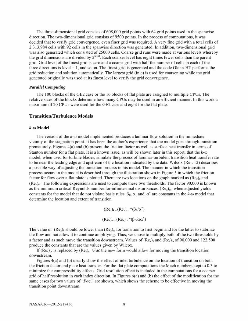
If (Rex)cr is replaced by (Rex)cr /Fac the new form would allow for moving the transition location downstream.

Figures 4(a) and (b) clearly show the effect of inlet turbulence on the location of transition on both the friction factor and plate heat transfer. For the flat plate computations the Mach numbers kept to 0.3 to minimize the compressibility effects. Grid resolution effect is included in the computations for a coarser grid of half resolution in each index direction. In Figures 6(a) and (b) the effect of the modification for the same cases for two values of “Fac,” are shown, which shows the scheme to be effective in moving the transition point downstream.

NASA/CR—2012-217436 9

Figure 5.—Skin friction variation for a boundary layer

undergoing transition from laminar to turbulent flow.

Figure 4(a).—Variation with grid resolution with the k- model on a flat plate.

Figure 4(b).—Variation with grid resolution with the k- model on a flat plate.

NASA/CR—2012-217436 10

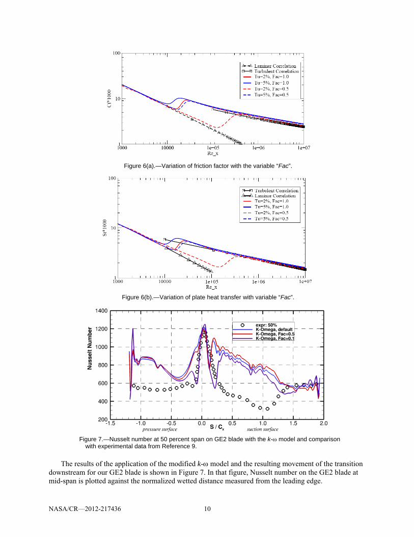
Figure 7.—Nusselt number at 50 percent span on GE2 blade with the k- model and comparison

with experimental data from Reference 9.

The results of the application of the modified k- model and the resulting movement of the transition downstream for our GE2 blade is shown in Figure 7. In that figure, Nusselt number on the GE2 blade at mid-span is plotted against the normalized wetted distance measured from the leading edge.

Figure 6(a).—Variation of friction factor with the variable “Fac”.

Figure 6(b).—Variation of plate heat transfer with variable “Fac”.

NASA/CR—2012-217436 11

Computations using the k- model designated as default version shows good match with the data at the leading edge. The agreement deteriorates soon after as the flow becomes fully turbulent in a short distance. For the two-dimensional computation of blade heat transfer on GE2 blade, the factor “Fac” causes the transition point to shift downstream. The fully turbulent flow results are not changed, as would be required by this modification, which is a good outcome. Unfortunately, although there is some effect on transition, the agreement with the data is not satisfactory and does not warrant adoption as a remedy.

Walters and Leylek Model

The model of Walters and Leylek (Refs. 5 and 6) has been developed with the process of transition built-in from the start. Walters and Leylek report that in developing the model their intention was for the model to be “hands off” for the user requiring no modification for different application cases. It is a phenomenological model as opposed to an empirically based model. It is a “single point” model and does not require non-local or integral quantities. That latter fact is an important enough quality that the model of Pacciani et al. (Ref. 7) was not chosen precisely because it requires quantities that were not “single point”. This is in spite of the fact that the results of application of the model to two-dimensional separated flows were shown in Reference 7 to be quite promising.

Low turbulence intensity in the free stream leads to natural transition of the boundary layer. With as low as 1 percent in intensity in free-stream turbulence, laminar velocity profile on the wall starts being affected by shifting momentum from outer region to inner region near the wall. Early attempts to model this effect relied upon turbulence diffusion and interaction with shear to promote transition. Experimental and computational evidence (Ref. 13) suggest that for the bypass transition the process of diffusion and interaction with shear may not be the governing mechanism. Large amplitude and low frequency streamwise fluctuations lead to increase in friction and wall heat transfer resulting in bypass transition as these streamwise fluctuations grow and breakdown. The low frequency aspect is critical. Shown by Moss and Oldfield (Ref. 14), the wall heat transfer does not respond to high frequency spectra in the free stream whereas the low frequency oscillations produces an increase in the level of wall heat transfer. Called the “Splat Mechanism,” described again by Bradshaw (Ref. 15), Volino and Simon (Ref. 16) by measuring the spectra of fluctuations in the free stream and in the boundary layer showed, that –uv in the boundary layer upstream (in the pre-transitional region) occurs at the same frequency as v in the upstream and thus is responsible for these oscillations.

Boundary layer flow is selective to certain free stream eddy scales and low-frequency disturbances in the boundary layer are amplified by the mean shear. The dynamics embodied in these streamwise fluctuations, in the model of Walters and Leylek, is captured by a “Laminar Kinetic Energy” equation through a modification of the concept devised by Mayle and Schulz (Ref. 17). Splats occur only for eddies with large length scales relative to the wall distance. Walters and Leylek have distinguished a “wall limited” large scale and “non-wall limited,” or small scale eddies in the near wall region as shown from Figure 8 taken from Reference 5. The effective eddy size designated in that figure delineates between larger eddies that contribute to the laminar kinetic energy (kL) and smaller ones that contribute to the turbulence. Transfer of energy from the laminar kinetic energy to the turbulent fluctuations initiates start of transition once a threshold is reached. Additional measures are implemented in the model to allow for natural and mixed mode transition. The turbulence model originally (Ref. 5) consisted of transport equations for Laminar, and turbulent kinetic energy, and rate of dissipation of kinetic energy of turbulence, kL, kT, and In a later paper (Ref. 6), the transport equations solved were modified to include the inverse turbulent time scale in place of It is suggested in Reference 6, that the latter form leads to a better representation of the breakdown of laminar kinetic energy to turbulence. This form of equations, but in compressible form, was implemented in the Glenn-HT codeThe form is given in Equation (1).

NASA/CR—2012-217436 12

Figure 8.—Delineation of scales relevant to production of laminar and turbulent kinetic energy, from Reference 5.

SC

RRk

CPxx

uxt

DRRPx

k

xuk

xt

k

DRRPx

k

xuk

xt

k

NATBPT

Rj

T

jj

j

TNATBPkTj

T

K

T

jjT

j

T

LNATBPklj

l

jjl

j

l

22

(1)

ρkl and ρkT are production terms for laminar and kinetic energy and consist of interaction of pre-transitional and turbulent Reynolds stresses with mean shear. Terms such as RBP and RNAT appear with opposite sign in the two equations for the laminar and turbulent kinetic energy equations and their role is to transfer the parts of laminar kinetic energy related to natural and bypass transition to turbulent kinetic energy. The complete form and details may be found in Reference 6 and the code Glenn-HT.

Some Aspects of the Implementation of the Model

The model was implemented into NASA’s Glenn-HT code. As the code is primarily an explicit code, the model equations were also implemented in an explicit manner. There are particular considerations about the implementation of the present model that will be briefly addressed.

Computation of distance to the wall had to be added to the code as the FORTRAN 90 version of Glenn-HT did not include this computation. The basic k- model which was the default turbulence model of that version of the code does not use the distance to the wall. Computation of wall distance as implemented is exclusively done for blocks having a wall boundary. For blocks having more than one wall boundary, the square root of the harmonic average of the individual square of the wall distances was used for the effective quantity. For blocks, not having a wall boundary the wall distance was designated as “very large.” As such, some care needs to be exercised in the process of grid generation not to develop meshes that have blocks neighboring walls that are too thin. As the wall distance within a block covers several orders of magnitude, the practical implementation of this requirement is not very restricting.

NASA/CR—2012-217436 13

Three variables (instead of one) had to be defined for the eddy viscosity, turbulence diffusivity, and turbulent thermal diffusivity as required by the model. The standard method is to use the eddy viscosity and use turbulent Prandtl number and Schmidt number to model other rates.

Additional model-specific variables were defined to house the above and additional variables to carry the “jacobian” of the source terms. It was determined that the jacobian was only necessary for equation.

The model calls for Neumann boundary conditions for Laminar Kinetic Energy, Turbulent kinetic energy and rate of dissipation on the walls as well as Dirichlet boundary conditions for laminar and turbulent kinetic energies. This over-specification was thought to be unsound and as it is the standard practice, we decided to use Neumann boundary conditions for the kinetic energies and Dirichlet for the rate of dissipation.

The CFL was reduced by a factor of 0.5 for the three turbulence model equations to improve the stability of the solution process. At present, there is no unusual limitation on CFL.

Residual smoothing which is an important tool for allowing larger time steps does not work well for the turbulence model equations and thus was not applied to them.

Source code is available on NASA computers.

Validation Results

Flat Plate Case

The plots of Cf (coefficient of friction) and Stanton number for flow over a flat plate are shown in Figures 9(a) and (b). The plot of Figure 9(a) shows the variation of friction factor, Cf = w/(0.5 u∞

2), or normalized wall shear stress by the dynamic head against the local Reynolds number. Each figure presents two inlet turbulence intensities as computed on two different grid refinement levels. Again, Mach number is held at 0.3 to reduce compressibility effects. The lines show that the computed location of transition is dependent on the grid resolution but the levels for the turbulent values are well predicted. As shown in Figure 9(a), the results of Cf show very good match to both the theoretically based laminar flow solutions and to measured turbulent flow values reported in Reference 10. The plot showing the variation of Stanton number with the local Reynolds number also shows a good match with the turbulent flow correlation reported in Reference 10. Agreement with the laminar flow heat transfer theory is imperfect showing enhancement in the laminar regime. This may be due to the explicit dependence of the turbulent thermal diffusivity on the laminar kinetic energy. The location of transition shows a physical movement upstream with increase in turbulence intensity, which is physically correct. The fully turbulent regime agrees with turbulent correlations quite well.

The results appear to make physical sense and agreement with theory and correlations is such that we can turn our attention to the turbine blade cascade comparison of GE2 geometry.

GE2 Blade Comparisons

Two-dimensional and three-dimensional runs were made to compare with mid-span and off mid-span results of GE2 experiment. As is the case with Glenn-HT code, the computations may be made at various levels of refinement to ensure grid convergence.

Pressure

Figure 10 shows the pressure distribution on the blade. Two-dimensional and three-dimensional results are shown. Three-dimensional results show better agreement with data. This is expected because in the experiment, the hub endwall had a thick boundary layer of 37 percent of half span and thus the pressure distribution from a two-dimensional computation should not match the three-dimensional run. Three-dimensional runs take the endwall boundary layer into account, which leads to better agreement with the experimental data at midspan.

NASA/CR—2012-217436 14

Figure 10.—Two-dimensional (left) and three-dimensional (right) computation of pressure distribution at the

midspan of GE2 blade and comparison with data from Reference 9.

Nusselt Number

In this section, we present two-dimensional (Fig. 10) and three-dimensional (Fig. 11) results for heat transfer for the GE2 blade. In these figures, the ordinate is the Nusselt number and the abscissa is the dimensionless wetted distance on the blade surface. Because of the prismatic shape of the blade, there is no ambiguity in the definition. The origin is the stagnation point defined based on the inlet angle. The

Figure 9.—Computations and comparison with data. (a) Friction factor.

(b) Heat transfer on a flat plate.

NASA/CR—2012-217436 15

definition of Nusselt number used to represent the dimensionless rate of heat transfer bears some description. Nusselt number is defined as:

k/hCNu xCx (2)

where Cx is the axial chord of the blade, k is the thermal conductivity of the fluid and h is the heat transfer coefficient defined as:

waw

w

TT

qh

(3)

In the above, qw is the wall heat flux; Tw and Taw are the wall and the recovery temperatures, respectively. The Taw in the experiment reported in Reference 9, was computed by an expression involving the recovery factor computed from,

31Pr /r (4)

where Pr, Prandtl number, is a physical property of the fluid. Using this relationship, the equation for the recovery temperature is:

2M

2

11 issaw rTT

(5)

M is the isentropic Mach number and is computed from the local wall pressure and inlet total pressure. Ts is the isentropic static temperature corresponding to the given Mach number. Given the above and the wall heat flux, the Nusselt number (Nu) can be computed. In the post-processing step, the local Mach number based on the local pressure ratio is computed and used to compute the adiabatic wall temperature.

Two-Dimensional Runs

Figure 11 shows the results obtained for heat transfer. A series of grid resolutions from coarse to fine grid are used. The data are included for comparison. A turbulence intensity of 13 percent and length scale of 1 percent of chord were specified at the upstream boundary. Grid convergence shows that fine grid (9500 points in two-dimensional) is needed for spatial convergence. On the “medium” grid the levels of laminar and turbulent heat transfer are well-predicted but for the location of transition to “settle” a finer grid is needed. The “fine” and “very fine” grids have, as described earlier, 9500 and 25,000 points. The predicted suction side heat transfer, similar to the experimental data, exhibits transitional behavior for which the location and extent of the transition agrees with the data. On the pressure side, the agreement is not as good, although the trend of heat transfer improves in agreement with the data as the grid is resolved further.

NASA/CR—2012-217436 16

Figure 11.—Two-dimensional computation of Nusselt number against data of

Giel et al. (Ref. 9), Re2 = 375 k.

Figure 12.—Three-dimensional computation of Nusselt number, midspan results and

comparison with data from Reference 9, Re2 = 375 k.

Three-Dimensional Runs

Midspan Nusselt number predictions are shown in Figure 12. The inlet turbulence was measured to be 13 percent in the experiment and the inlet boundary layer thickness on the endwall is reported to be 37 percent of half span. A length scale of 1 percent span was used for the turbulence length scale. The computations were carried out on three grids of varying densities. The same grids shown in Figures 3(b) and (c) are used for three-dimensional computations. The grid in 3(c) (2.3e6 grid points) was used for coarsening while the grid in 3(b) (610,000 grid points) was used on the finest level to verify convergence. The solution on the fine grid slightly differs from the medium grid as it concerns the transition location. The magnitude of Nusselt number is seen to be somewhat under-predicted. As shown in Figure 13, both a 1 and 10 percent of span for the length scale was tried. The 10 percent length scale was used in the hope of improving the results on the pressure side and in the fully turbulent regime but the 1 percent scale had a better agreement. Figure 14 presents comparison with experimental data for the 15, 25, and 50 percent span for the two finest grids. Comparisons are provided to show that using the “Fine” grid, grid convergence has been achieved. For all the span locations, heat transfer in the fully turbulent regime downstream on the suction side is under-predicted. The transition location, however, is quite accurately predicted. Figure 15, shows the Nusselt number, as a contour plot over the blade, seen on a coordinate system consisting of surface distance measured from the leading edge on the abscissa and the spanwise distance on the ordinate. Similar to the experimental data, near the hub endwall, the Nusselt number rises to quite large values. The extent of the elevated region in the model is less than in the experiment. Given the very good agreement with the data for the midspan for the two-dimensional computation, it may be concluded that the extent of the three-dimensional effect of the endwall boundary layer may be over-

NASA/CR—2012-217436 17

estimated. This may be due to inadequacy in the turbulence model or it may be input inaccuracies such as the input boundary layer thickness values or differences in the shape of the inlet profile between the assumed and the actual. (In the computations, a flat plate turbulent boundary layer profile was assumed.)

The present work-plan called for the choice of a turbulence model with good transition pre-diction capabilities. The foregoing shows that the Walters-Leylek model possesses the desired capabilities. We did not perform an exhaustive survey of all the candidates but this could be an item of research in the future.

Figure 13.—Effect of the applied turbulent length scale at the inlet against data of Giel et al. (Ref. 9), Re2 = 375 k.

Figure 14.—Three-dimensional computation of Nusselt number and comparison with data of Giel et al. (Ref. 9), Re2 = 375 k.

NASA/CR—2012-217436 18

Figure 15.—Contour plot of Nusselt number over the surface of the vane, Re2 = 375 k top figure is from experiments

(Ref. 9) and the bottom figure is from present computations.

Numerical Prediction of Aerodynamic Losses

We next turned our attention to the computation of the “loss bucket” for the candidate case. The candidate case is the data-set of Giel and McVetta (Ref. 18). This data-set has surveys of the exit total pressure of a linear cascade which has have been taken at for a wide variation of incidence angles. The data was used to help verify the loss prediction capability, in particular for large angles. The data of Giel and McVetta were taken in NASA Glenn’s CW22 transonic cascade tunnel. The blade profile is from the E3 tip profile (Ref. 18). In addition to the losses, measurements are available for blade tip heat transfer. The data used for this work was for zero tip clearance. In the sections below, we will describe the experimental and numerical setups used in this study.

NASA/CR—2012-217436 19

Validation Results

Loss computations were validated using the data obtained in the Transonic Cascade at NASA Glenn Research Center. The effort is described in the following.

Experimental Data of Giel and McVetta

Giel and McVetta used the near tip profile of the GE-E3 blade (Ref. 19) in a linear cascade. They measured the total pressure at near 9 percent of axial chord downstream of the blade. The loss coefficient Cp was computed using the following formula:

2_

__

sint

xtintp PP

PPC (6)

Here the subscripts “t” signifies total value and the subscripts “x” and “in” signify local and inlet values. At the inlet, the incoming flow was low turbulence and the boundary layer was 25 percent of span in thickness. The Reynolds number for the case of our interest, based on the incoming velocity and the chord, was 85,000. The computed losses are for Reynolds numbers of 85,000. Loss data are available for the Reynolds number of 85,000 at the midspan of the channel and for four different incidence angles. Losses are due to thickening of boundary layers as well as transition from laminar to turbulent flow and separation. Figure 16 shows the measured midspan loss coefficient at a station (x) located at 0.086x axial chord downstream of the trailing edge of the cascade. As shown, the losses increase as the incidence angle increases beyond (–5). Although this incidence angle is specified as negative, it produces the lowest losses. The choice of zero, at this juncture, is not very important. In the next section, we will present computation of the losses and comparison with the experimental data of Figure 16.

Figure 16.—Losses at mid-span of linear cascade with the E3 blade tip profile for

Reynolds number of 85,000 (Ref. 18).

NASA/CR—2012-217436 20

(a) (b)

Figure 17.—(a) Three-dimensional blade grid of the E3 blade tip section cascade.(b) A two-dimensional section at the hub showing the grid resolution.

Computation Details

In the next section the grid produced for this geometry is defined. For the computations at the inlet a boundary layer thickness equivalent to 25 percent tunnel span was specified. Angles at the inlet were varied to match the case being computed. The inlet turbulence intensity was specified at 1 percent and length was specified at 1 percent of axial chord. At the exit a pressure ratio of 0.925 was specified. Grid for E3 Blade Tip Section

Flow in the linear cascade of the E3 tip profile was simulated in order to reproduce the losses from the experiment of Giel and McVetta, shown in Figure 17.

Previous experience shows that a fine grid would be required for loss computations. A grid with 2.75e6 points, as shown in Figure 17 was generated for this purpose. A two-dimensional section of the grid being stacked 81 times contains 34,000 grid points. Again, as it was discusses in connection with GE2 blade gridding, upstream boundary of the grid was matched with the experimental measuring station upstream where the conditions were measured.

Computed Loss Profiles Downstream

Figure 18 shows the losses as computed using the once coarsened grid (340,000 points) and Figure 19 shows the same on the finest level grid. As mentioned earlier, the grid used for Figure 19 is eight times denser than the one used in Figure 18. Given that the Reynolds number is quite small, the grid resolution is expected to be very fine. However, a yet finer grid is required to “prove” that the results are grid independent. Figure 19, shows the loss profiles for a Reynolds number of 85 k corresponding to the data. The four measured incidence angles are included. The measurements were performed only at the midspan but they were done over three pitches, hence the variation in the data from pitch to pitch. Computation results are simply repeated as they were done for one period. For the two larger incidence angles, the figure shows excellent agreement with the data at the largest incidences. The agreement is not as good for the smaller incidences and the two-dimensional losses are under-predicted. The larger of the two incidence angles form zones of separation and deviate greatly from ideal flow angles. The worst case corresponds to the baseline case. Inspection of results shows that the computations at the midspan do not show any separation at the baseline and are nicely attached as with the case of baseline incidence.

NASA/CR—2012-217436 21

Figure 18.—Losses computed on the coarse grid, Re = 100 k.

Figure 19.—Predicted total pressure loss coefficient on level 0 grid at Re = 85 k.

NASA/CR—2012-217436 22

Figure 20.—Total pressure loss contours for incidences of 0 (left) and 20 (right).

Figure 21(a).—Loss coefficient iso-surface of 0.5 for the 0 incidence angle and (b) Loss coefficient iso-surface of

0.7 for the 20 incidence angle. Colored by density.

To understand better the losses and the sources of loss we refer to Figure 20. In that figure, two plots are made for the loss coefficient contours downstream of the blades (at 1.086 axial chord from the leading edge) for two incidence angles of 0 and 20. Areas of large total pressure loss are shown in red. The upper values of the contours are near the highest values attained by the experimental data for each case in the line plot. There are three areas of large loss values that can be identified for each case in these figures. One area of increased losses may be found near the endwall and appear to develop from interaction of the endwall boundary layer and the wake of the blade. The second area appears to be due to the pressure side leg of the horseshoe vortex and is situated in the middle of the (half) passage and are shown in Figures 21(a) and (b). A third region of large losses is shown at midspan for the 20 case and near midspan for the smaller incidence angle. The suction side leg of the horseshoe vortex forms this. For the large incidence case, the flow initially separates on the suction side but reattaches. It was thought by the author that the blade flow at midspan, on the suction side, would be completely separated. A thorough inspection of the flow shows this not to be the case. Flow separation at midspan is confined and the flow does reattach. It is hypothesized that the losses are principally associated with the large region of secondary flow within the passage and blade boundary layer/secondary vortex interaction. The larger the incidence, the larger the effect of secondary flow caused by the loading of blades. For the (–5) the losses are low as predicted.

(a) (b)

NASA/CR—2012-217436 23

Integrated Results

Losses for the cases computed in Figure 19, as well as an additional computation for the incidence angle of –10, were averaged over the exit channel area at the measuring station (x = 1.086x Cx) in order to compute an average loss coefficient. Area averaging was used to account better for losses in locations with low mass flow or where flow reversal may exist. The resulting line plot of the integrated losses against the incidence angle, as shown in Figure 22, is what is referred to as a loss bucket. The results show the minimum loss to occur at an incidence of –5. This corresponds to an inlet angle of 33.8.

Welch (Ref. 1) presented the loss bucket for high-lift rotor blading of Clark et al. (Ref. 20). Figure 23 was taken from (Ref. 1) which shows the losses for two different Reynolds numbers. Cruise (design air angles) and take-off (–50 incidence) operations are also marked and the flow visualization shown as insets to the figure. Angle condition at take-off induces a large cove separation on the pressure side (Ref. 21) which will be computed later in this work. The plot can be used to check the validity of the analysis as performed here once the loss bucket is fully populated. At the present stage of the work, it appear that the losses for the present computations are higher than those of Figure 23. This may be reasonable as results presented herein include the full three-dimensional losses, and include endwall and secondary flow losses which contribute to the integrated values. The computations in Reference 1 were performed using a two-dimensional Navier-Stokes analysis and a low Reynolds number k- model. The agreement appears to be reasonable. It bears reminding the reader that the inlet boundary layer thickness for the cascade of Giel and McVetta was quite substantial and as such the computations of losses for this cascade does not lend itself to two-dimensional analysis.

Figure 22.—Loss bucket formed from the three-dimensional loss integration of Figure 17.

NASA/CR—2012-217436 24

Figure 23.—Loss bucket from Reference 1.

Summary

For the Variable Speed Power Turbine work, the flow transition/separation has been identified as an important process. Computational schemes need to address this question if the losses are to be predicted correctly. Under the present task, the literature was surveyed and the model of Walters and Leylek (Ref. 6) was chosen as a suitable candidate. This model uses a phenomenological model of the bypass transition. The work presented herein, describes the performance of the low Reynolds number k- model and Walters-Leylek three-equation model as it pertains to prediction of transition. The Walters-Leylek model was implemented in NASA Glenn-HT code and tested by applying to a turbine blade test case for heat transfer. The location of transition was successfully predicted on the suction side and the transition modeling on the pressure side was accurate. Both two-dimensional and three-dimensional computations were performed for this test. The model was then employed to compute the E3 tip profile cascade of Giel and McVetta. The midspan losses were computed successfully at large incidence angles and fairly well at lower incidences. The integrated losses were computed and used to form the loss bucket.

Future Work

Future work will look at further three-dimensional applications of the model to include the data of Giel and McVetta at higher Reynolds numbers. As for the loss bucket, incidence angles lower than –10 and similar to Figure 22 will be computed and included.

References

1. Welch, G.E., “Assessment of Aerodynamic Challenges of a Variable-Speed Power Turbine for Large Civil Tilt-Rotor Application,” Proc. AHS Forum 66, May, 2010; also NASA/TM—2010-216758, Aug. 2010.

2. Boyle, R.J. and Ameri, Ali A., “Grid Orthogonality Effects on Turbine Midspan Heat Transfer and Performance,” ASME Journal of Turbomachinery, 119, No. 1, pp. 31–38, Jan. 1997.

3. Suzen, Y.B., and Huang, P.G., 2000, “Modeling of Flow Transition Using an Intermittency Transport Equation,” ASME Journal of Fluids Eng., 122, pp. 273–284.

4. Steelant, J., and Dick, E., 2001, “Modeling of Laminar-Turbulent Transition for High Free-stream Turbulence,” ASME Journal of Fluids Eng., 123, pp. 22–30.

NASA/CR—2012-217436 25

5. Walters, D. Keith and Leylek, James H., 2004, “A New Model for Boundary Layer Transition Using a Single-Point RANS Approach,” ASME Journal of Turbomachinery, Volume 126, Issue 1, 193.

6. Walters, D. Keith and Leylek, James H., 2005 “Computational Fluid Dynamics Study of Wake-Induced Transition on a Compressor-Like Flat Plate,” ASME Journal of Turbomachinery—January 2005—Volume 127, Issue 1, 52 (12 pages).

7. Pacciani R., Marconcini M., Fadai-Ghotbi A., Lardeau S., Leschziner, M.A., 2011, “Calculation of High-Lift Cascades in Low Pressure Turbine Conditions Using a Three-Equation Model,” ASME Journal of Turbomachinery, 133, 031016 (2011). ISSN 0889-504X.

8. Ameri, A.A. and Arnone A., “Transition Modeling Effects on Turbine Rotor Heat Transfer,” ASME Journal of Turbomachinery, 118, No. 2, pp. 307–313, Apr. 1996.

9. Giel, Paul W., Boyle, Robert J. and Bunker, Ronald S., 2004, “Measurements and Predictions of Heat Transfer on a Transonic Turbine Cascade,” Journal of Turbomachinery, Volume 126, Issue 1.

10. Fundamentals of Heat Transfer, Incropera, Frank P. and DeWitt, David P., pp. 393–396, New York: Wiley, c1981.

11. Steinthorsson, E., Liou, M.S., and Povinelli, L.A., 1993, “Development of an Explicit Multiblock/Multigrid Flow Solver for Viscous Flows in Complex Geometries,” AIAA-93-2380.

12. Wilcox, D.C., Turbulence Modeling for CFD, 3rd edition, DCW Industries, Inc., La Canada CA, 2006.

13. Volino, R.J., 1998, “A New Model for Free-Stream Turbulence Effects on Boundary Layers,” ASME J. of Turbomachinery, 120, pp. 613–620.

14. Moss, R.W. and Oldfield, M.L.G. 1996, “Effect of Free-Stream Turbulence on Flat-Plate Heat Flux Signals: Spectra and Eddy Transport Velocities,” ASME Journal of Turbomachinery, Volume 118, Issue 3, 461.

15. Bradshaw, P., 1994, “Turbulence: The Chief Outstanding Difficulty of Our Subject,” Exp. Fluids, 16, pp. 203–216.

16. Mayle, R.E., and Schulz, A., 1997, “The Path to Predicting Bypass Transition,” ASME Journal of Turbomachinery, 119, pp. 405–411.

17. Volino, R.J., and Simon, T.W., 1997, “Boundary Layer Transition Under High Free-Stream Turbulence and Strong Acceleration Conditions: Part 2—Turbulent Transport Results,” ASME Journal of Heat Transfer, 119, pp. 427–432.

18. Giel, P.W. and McVetta, A., Unpublished loss data and exit angle measurements for E3 tip section. 19. Timko, L.P., “Energy Efficient Engine High Pressure Turbine Component Test Performance

Report,” NASA CR-168289, 1984. 20. Clark, J.P., Koch, P.J., Ooten, M.K., Johnson, J.J., Dagg, J., McQuilling, M.W., Huber, F, and

Johnson, P.D, “Design of Turbine Components to Answer Research Questions in Unsteady Aerodynamics and Heat Transfer,” AFRL-RZ-WP-TR-2009-2180, (Internal Report) Sept. 2009.

21. Welch, G.E., 2011, “Computational Assessment of the Aerodynamic Performance of a Variable-Speed Power Turbine for Large Civil Tilt-Rotor Application,” Proceedings AHS Forum 67, Virginia Beach, VA, May 3-5, 2011; also NASA/TM—2011-217124.

REPORT DOCUMENTATION PAGE Form Approved OMB No. 0704-0188

The public reporting burden for this collection of information is estimated to average 1 hour per response, including the time for reviewing instructions, searching existing data sources, gathering and maintaining the data needed, and completing and reviewing the collection of information. Send comments regarding this burden estimate or any other aspect of this collection of information, including suggestions for reducing this burden, to Department of Defense, Washington Headquarters Services, Directorate for Information Operations and Reports (0704-0188), 1215 Jefferson Davis Highway, Suite 1204, Arlington, VA 22202-4302. Respondents should be aware that notwithstanding any other provision of law, no person shall be subject to any penalty for failing to comply with a collection of information if it does not display a currently valid OMB control number. PLEASE DO NOT RETURN YOUR FORM TO THE ABOVE ADDRESS.

1. REPORT DATE (DD-MM-YYYY) 01-04-2012

2. REPORT TYPE Final Contractor Report

3. DATES COVERED (From - To)

4. TITLE AND SUBTITLE Implementation of a Transition Model in a NASA Code and Validation Using Heat Transfer Data on a Turbine Blade

5a. CONTRACT NUMBER NNC06BA07B

5b. GRANT NUMBER

5c. PROGRAM ELEMENT NUMBER

6. AUTHOR(S) Ameri, Ali, A.

5d. PROJECT NUMBER

5e. TASK NUMBER NNC10E420T-0

5f. WORK UNIT NUMBER WBS 877868.02.07.03.01.02.01

7. PERFORMING ORGANIZATION NAME(S) AND ADDRESS(ES) The Ohio State University

8. PERFORMING ORGANIZATION REPORT NUMBER E-18129

9. SPONSORING/MONITORING AGENCY NAME(S) AND ADDRESS(ES) National Aeronautics and Space Administration Washington, DC 20546-0001

10. SPONSORING/MONITOR'S ACRONYM(S) NASA

11. SPONSORING/MONITORING REPORT NUMBER NASA/CR-2012-217436

12. DISTRIBUTION/AVAILABILITY STATEMENT Unclassified-Unlimited Subject Categories: 07 and 34 Available electronically at http://www.sti.nasa.gov This publication is available from the NASA Center for AeroSpace Information, 443-757-5802

13. SUPPLEMENTARY NOTES

14. ABSTRACT The purpose of this report is to summarize and document the work done to enable a NASA CFD code to model laminar-turbulent transition process on an isolated turbine blade. The ultimate purpose of the present work is to down-select a transition model that would allow the flow simulation of a variable speed power turbine to be accurately performed. The flow modeling in its final form will account for the blade row interactions and their effects on transition which would lead to accurate accounting for losses. The present work only concerns itself with steady flows of variable inlet turbulence. The low Reynolds number k-ω model of Wilcox and a modified version of the same model will be used for modeling of transition on experimentally measured blade pressure and heat transfer. It will be shown that the k-ω model and its modified variant fail to simulate the transition with any degree of accuracy. A case is thus made for the adoption of more accurate transition models. Three-equation models based on the work of Mayle on Laminar Kinetic Energy were explored. The three-equation model of Walters and Leylek was thought to be in a relatively mature state of development and was implemented in the Glenn-HT code. Two-dimensional heat transfer predictions of flat plate flow and two-dimensional and three-dimensional heat transfer predictions on a turbine blade were performed and reported herein. Surface heat transfer rate serves as sensitive indicator of transition. With the newly implemented model, it was shown that the simulation of transition process is much improved over the baseline k-ω model for the single Reynolds number and pressure ratio attempted; while agreement with heat transfer data became more satisfactory. Armed with the new transition model, total-pressure losses of computed three-dimensional flow of E3 tip section cascade were compared to the experimental data for a range of incidence angles. The results obtained, form a partial loss bucket for the chosen blade. In time the loss bucket will be populated with losses at additional incidences. Results obtained thus far will be discussed herein.15. SUBJECT TERMS Power turbine; Low pressure turbine; Turbulence modeling; Heat transfer losses

16. SECURITY CLASSIFICATION OF: 17. LIMITATION OF ABSTRACT UU

18. NUMBER OF PAGES

31

19a. NAME OF RESPONSIBLE PERSON STI Help Desk (email:help@sti.nasa.gov)

a. REPORT U

b. ABSTRACT U

c. THIS PAGE U

19b. TELEPHONE NUMBER (include area code) 443-757-5802

Standard Form 298 (Rev. 8-98)Prescribed by ANSI Std. Z39-18