Implementation and Application of Methods for Micro

Implementation and Application of Methodsfor Micro-Gravity Emulation

by

Thomas Richard Johnstone Corrigan

Bachelor of Science in Mechanical EngineeringUniversity of Minnesota (1992)

Bachelor of Science in Applied PhysicsSaint John's University (1992)

Submitted to theDepartment of Mechanical Engineering

in partial fulfillment of the requirements for the degree of

Master of Science in Mechanical Engineering

at the

Massachusetts Institute of Technology

September 1994

© 1994 Massachusetts Institute of Technology

Signature of

I..

,Cerifidb - A(} Steven Dubowsky

Thesis Supervisor

Accepted by . .. _Ain A. Sonin

Chairman, Departmental Graduate Committee

UBRA~t

Certified by

2

Implementation and Application of Methodsfor Micro-Gravity Emulation

Submitted to theDepartment of Mechanical Engineering

in partial fulfillment of the requirements for the degree ofMaster of Science in Mechanical Engineering

by

Thomas Richard Johnstone Corrigan

AbstractExperimentally evaluating micro-gravity control and planning algorithms

for space robotic systems on earth is difficult because gravity masks the moresubtle dynamic forces which dominate in space. Previous experimental test bedsfor micro-gravity have been largely restricted to planar motion, or have otherlimitations. A system called the Vehicle Emulation System (VES), a fully spatialsystem, overcomes many of these problems. However, compensating for theeffects of gravity with the VES is a challenge.

This thesis presents two methods of gravity compensation, the LearningMethod and the Model Method, which allow fully spatial emulation of the micro-gravity interaction between a space manipulator and its supporting structure orspacecraft. Experimental results show the effectiveness of the methods.

These micro-gravity emulation techniques are used to experimentallyevaluate the effectiveness of two space robotic algorithms, the Coupling MapAlgorithm and the Pseudo-Passive Energy Dissipation Concept.

Finally, the design and evaluation of a digital filter which improved theperformance of the VES system is presented.

Thesis Supervisor: Dr. Steven DubowskyProfessor of Mechanical Engineering

__

4

Acknowledgments

I will always be grateful to my advisor, Professor Steven Dubowsky, forgiving me one of the greatest opportunities of my life. His guidance and advice,in engineering, professionalism, communication and life itself will stay with meforever.

I would like to thank my predecessors in the group who made mytransition to MIT an enjoyable experience. They are Andrew Kuklinski, DalilaArgaez, Chantal Moore, Peng Yun Gu, Miguel Torres, Joe Deck, and AttilioPissoni. I would especially like to thank Andrew and Dalila for filling my firstyear at MIT with adventures, lots of laughs, and a fair amount of goofingaround.

I thank Craig Sunada whose entrance to the group--as well as marriedlife--coincided with mine, for providing camaraderie and friendship. Thank youto the students who joined the group after me--Jeff Cole, Nathan Rutman,Richard Wang and Michele Tesciuba--for making me feel like I knew what wasgoing on once in a while, and for making the lab and office enjoyable.

To my loving wife Mary I owe the greatest thanks for supporting methrough countless hours of research, and for inspiring me to pursue excellence.Consider this a toast.

To my Parents I owe a great deal of thanks; for providing the genetic andeducational framework for success, and for a life time of unconditional love andsupport. I would also like to thank my brother Pat and sisters Beener, Bell, andKaz for their support, and for making my life more interesting. I would like tothank my two best friends, Kevin Davis and Terry Szymanski, for spendingcountless hours keeping me in touch (electronically) with my home.

I would like to recognize the efforts of the professors and students whoproceeded me in the VES project and made my own research possible. Theyinclude Professor Will Durfee, Professor Igor Paul, Uwe MUiller, Husni Idris, JayBaker, and Andrew Kuklinski. The support of NASA grant NAG-1-801 for thiswork is also recognized.

Acknowledgments 5

6

Table of Contents

1 Introduction 13

1.1 Background and Literature Review .................................... .... 13

1.2 Purpose of this Thesis................................................15

1.3 Outline of Thesis................................................... ........... ............ 16

2 The Experimental System 19

2.1 Introduction .............................................................. 19

2.2 The VES Basic Operation............................................. 19

2.3 The Admittance Control Concept ..................................... ..... 22

2.4 The VES Control Architecture ........................................ ..... 252.4.1 An Overview ............................................ ......... .......... 252.4.2 The Platform Admittance Control Cycle......................... 272.4.3 PUMA 560 Control....................... ....... 29

2.5 Sum m ary ................................................... ............................................ 30

3 Emulating Micro-Gravity 31

3.1 In troduction ...................................................................... .................... 31

3.2 The Challenges of Micro-Gravity Emulation........................... ... 323.2.1 Wrench Error Sensitivity...................................323.2.2 Position Error Sensitivity .................................... ..... 333.2.3 Required Estimation Accuracy ...................................... 343.2.4 Error Sources ................................................... 35

3.3 Learning Method Gravity Compensation ...................................... 373.3.1 The Learning Algorithm ...................................... .... 383.3.2 Em ulation A ccuracy .................................................................... 40

3.4 Model Method Gravity Compensation.......................... ...... 413.4.1 Determining Mass Parameters.......................... ..... 423.4.2 Formulating the Model ...................................... ..... 433.4.3 Estimating Gravity Forces ..................................... .... 443.4.4 Estimating Gravity Moments.............................................453.4.5 From Theory to Application......................... ....... 483.4.6 Emulation Accuracy ....................................... ....... 51

3.5 Comparison of the Methods ........................................ ....... 53

3.6 Sum m ary................................................... ............................................ 55

Table of Contents

4 Investigation of Planning and Control Methods 57

4.1 In trod u ction ................................................................................................ 57

4.2 The Coupling Map ....................................................... 58

4.3 Pseudo-Passive Energy Dissipation ..................................... .... 624.3.1 The Virtual Manipulator Simplification.................. 634.3.2 Full Dynamic Analysis ....................................... ..... 65

4.4 Sum m ary ................................................... ............................................ 70

5 Improving System Performance with a Digital Filter 71

5.1 Introduction ...................................................................... .................... 71

5.2 The Performance Problems................. ............... 71

5.3 The D esign Solution................................................................................ 73

5.4 Effect of Filter Location on Stability ..................................... .... 76

5.5 D igital Filter Results............................................................................ 79

5.6 Choosing Platform Gains ................................................. 81

5.7 Sum m ary ................................................... ............................................ 83

6 Conclusions 85

6.1 Contributions of This W ork .................................................................. 85

6.2 Recommendations for Future Work ..................................... .... 86

Bibliography 89

A Modeling Beam Structures 95

A.1 Introduction .............................................................. 95

A.2 Modeling a Straight Beam ................................................. 95

A.3 Straight Beam Experiments ................................................ 97

A.4 Modeling a Complex Beam .................................................................... 101

A.5 Complex Beam Experiments........................................103

B The Anatomy of a PUMA 560 105

B.1 Coordinates and Definitions ................................................................... 105

B.2 Link Masses and Inertias .................................................................... 106

B.3 Homogeneous Transformation Matrices.............................................107

B.4 Jacobian Matrices ........................................................ 108

B.5 Virtual Manipulator to Endpoint ........................................................... 109

Table of Contents

B.6 Virtual Manipulator to Base ......................................... ...... 110

C Modeling a PUMA 560 111

C .1 Introduction ........................................... ............................................... 111

C.2 Evaluating the P vector ................................................... 111

C.3 Experimental Versus Measured Mass Parameters ............................. 115

D Coordinate Frame Transformation 116

E The VES Micro-Gravity Handbook 117

E.1 Introduction .............................................................. 117

E.2 VES II Basic Rules ..................................................... ......... .......... 117

E.3 Basic Operating Procedures........................ ...... ................. 118

E.4 Laboratory Arrangement...........................................126

F Force Sensor Noise 128

G Linearized Dynamic Model of PUMA on a Flexible Base 131

Introdu ction ..................................................... .............................................. 131

T h e M od el ...................................................... ................................................ 131

Table of Contents

10

List of Figures

Figure 1-1: Space Manipulator System Concept............................. ..... 14

Figure 2-1: The VES II with a PUMA 560 ....................................... ...... 20

Figure 2-2: VES Admittance Mode Schematic............................. ...... 21

Figure 2-3: VES Micro-Gravity Emulation Mode Schematic........................ 22

Figure 2-4: Platform frames and rotation axes ..................................... .... 23

Figure 2-5: Typical VES Space Robotic System ..................................... .... 25

Figure 2-6: VES Computer Architecture................................ ....... 26

Figure 2-8: Admittance Control Cycle ............................................... 28

Figure 3-1: Dynamic Wrench Vectors with Gravity Error Ranges....................33

Figure 3-2: Micro-Gravity Motions with AVrg Errors.............................. .... 34

Figure 3-3: Learning Algorithm Schematic ....................................... .... 39

Figure 3-4: Rotation of Base During Learning Iterations.....................................41

Figure 3-5: Link "i" center of mass vector................................. ...... 45

Figure 3-6: Estimated and Actual Gravity Wrench ...................................... 53

Figure 3-7: Micro-Gravity Moment ................................................. 55

Figure 3-8: Micro-Gravity Rotation .......................................... ....... 55

Figure 4-1: Coupling Map Cross Sections for PUMA 560 on Flexible Beam........60

Figure 4-2: Energy Transferred to the Flexible Beam for Two Motions............61

Figure 4-3: Energy Transferred to Beam With and Without Gravity ................62

Figure 4-3: Virtual Manipulator Modeling Concept ........................64

Figure 4-4: System Poles, PPED Gains ....................................... ....... 67

Figure 4-5: System Poles, High Gains ......................................... ...... 68

Figure 4-6: PPED Simulation Results, Translation ................................................69

Figure 4-7: PPED Simulation Results, Energy........................................................69

Figure 5-1: Platform leg natural frequencies. .......................................................72

List of Figures

Figure 5-2: Original closed loop response with high and low gains..................72

Figure 5-3: Basic filter types, corner frequency of 10Hz ..................................... 73

Figure 5-4: Closed Loop Actuator Block Diagram ......................... 74

Figure 5-5: Experimental verification of open loop filter design ...................... 76

Figure 5-6: VES Admittance Control Block Diagram .............................................. 77

Figure 5-7: Digital Filter on Error Signal.................................... ...... 77

Figure 5-8: VES Pole Plot, Filter on Error Signal .................................... .... 78

Figure 5-9: Digital Filter on Feedback Signal ...................................... .... 78

Figure 5-10: VES Pole Plot, Filter on Feedback Signal........................................79

Figure 5-11: Platform positioning errors ....................................... ...... 81

Figure 5-12: Bode Plot of Platform with Filter ......................................... 82

Figure 5-13: Platform Unit Step Response with Filter ..................................... 83

Figure A-1: PUMA on Vertical Beam ......................................... ....... 97

Figure A-2: PUMA on VES Performing Simple Motion...............................99

Figure A-3: Position and Velocity Profiles of Simple Motion ............................... 100

Figure A-3: PUMA Complex Beam .......................................... ....... 104

Figure B-1: PUMA 560 D-H Parameters ........................................ ...... 105

Figure B-2: PUMA 560 link masses and position vectors ................................... 106

Figure B-3: PUMA 560 Virtual Manipulator to Endpoint........................................109

Figure B-4: PUMA 560 Virtual Manipulator to Base ....................................... 110

Figure D-1: Coordinate frame relationships ....................................... ..... 116

Figure E-1: Platform Arrangement in New Laboratory ......................................... 127

Figure F-1: High Frequency Sensor Noise - Force................................ .... 128

Figure F-2: High Frequency Sensor Noise - Moment ..................................... 129

Figure F-3: Low Frequency Sensor Noise - Force.............................. .... 129

Figure F-4: Low Frequency Sensor Noise - Moment .................................. 130

List of Figures

Chapter 1

Introduction

1.1 Background and Literature Review

The hazard and expense of space maneuvers makes extensive preflight

experimental testing of control and planning schemes for space robotics critical.

The gravity of earth dominates most dynamic systems, making micro gravity

emulation difficult.

In many proposed space applications there are important dynamic

interactions between a manipulator and its base structure [Umetani and

Holcomb 1990]. These applications include free floating systems, such as a robot

mounted on a small satellite, and free flying systems, where the robot-satellite

combination is positioned by reaction jets [Erickson et al 1989]. Another

important scenario is a space robotic manipulator carried by a long slender arm

from a base structure [Crane et al. 1991], such as the space manipulator system

idealized in figure 1-1.

A number of planning and control algorithms have been proposed for

robotic systems in the micro-gravity of space [Xu and Kanade 1993]. It is

relatively easy to test these algorithms in simulation; however, experimental

tests are required to validate their effectiveness fully. Performing such tests in

Chapter 1: Introduction

terrestrial laboratories is difficult since gravity often masks the dynamic effects

which dominate in the micro-gravity of space. For example, the dynamic forces

and moments exerted by a free flying space manipulator on its spacecraft can

cause undesirable system motions if these are not compensated for

Panalnnnllonsn and 1lDuhnwskv 19931LA GrCGAJrwA`-

Figure 1-1: Space Manipulator System Concept.

Each of the existing test bed systems developed to study the dynamics

and control of space manipulators in micro-gravity has advantages and

limitations. The most common systems use air bearings riding on a flat surface

to support a manipulator system [Alexander and Cannon 1990, Umatani and

Yoshida 1989]. These relatively simple and useful studies are restricted to planar

motion. But the complex nature of real space robotic systems makes their full

three dimensional behavior important. Neutral buoyancy tanks are used to

approximate three dimensional weightless motions [Spofford and Akin 1990].

These systems are effective for some studies, but fluid damping and inertia can

corrupt the results when a system's dynamic behavior is important. The


complexity of suspension systems with counterbalancing mechanisms proposed

for micro-gravity emulation makes their reliable, accurate use difficult at best

[Sato et al. 1991, Ulrich and Kumar 1991]. Finally, other systems only simulate

micro-gravity with approximations of a system's dynamics [Iwata et al. 1990,

Shimoji et al. 1989, Whittaker et al. 1991]. Complex three dimensional dynamic

interactions cannot be completely studied with any of these approaches.

A system called the Vehicle Emulation System Model II (VES) developed

at MIT permits the experimental evaluation of planning and control algorithms

for mobile terrestrial and space robot systems by using an approach called

"admittance control" [Fresko 1987].

1.2 Purpose of this Thesis

The VES II is a second generation experimental test bed, designed and

built to study experimentally the three dimensional motion of complex mobile

manipulator systems. An earlier version, the VES I was built in the 1980's and

used to study several manipulator control algorithms [Stelman 1988]. The VES II

was designed to investigate a wider range of dynamic systems with an increased

accuracy (Mtiller 1992, Idris 1992, Kuklinski 1993). With effective gravity

compensation, the VES II is now capable of emulating micro-gravity conditions.

Previous theses have detailed the design of the VES II hardware (Miiller

1992), the software used to control the VES II (Idris 1992), and the integration of

many components to get the system working well (Kuklinski 1993). This thesis

documents the final addition to the VES II system, the ability to emulate micro-

gravity environments to study space robotics. Two methods of compensating

for gravity are presented to achieve this emulation, the Learning Method and the

Model Method. Two control and planning algorithms for space robotics are

investigated with the VES II system to demonstrate the use of the gravity


compensation technology. The addition of a digital filter to improve the

performance of the system, is also documented. The equations used by the

gravity compensation methods are compiled in the appendices, along with a

detailed handbook for operating the VES II.

1.3 Outline of Thesis

This thesis is organized into 6 chapters. This chapter serves as an

introduction to set the background and purpose for the work. An overview of

the basic VES system is presented in Chapter 2. The hardware and software

architecture is summarized. The admittance model concept is also discussed.

Chapter 3 describes the inherent difficulties involved in emulating micro-

gravity. Two methods of emulating micro-gravity, the Learning Method and the

Model Method, are then presented in detail, along with some results which

demonstrate the accuracy of these methods.

Chapter 4 reviews space robotics control and path planning theories and

applies the VES to analyzing two of them, the Coupling Map Algorithm and

Pseudo-Passive Energy Dissipation.

The design and implementation of a digital filter is presented in Chapter 5.

The improvements achieved by this filter are also documented.

An extensive series of appendices provides some details of this work. The

calculations for generating an admittance model of a beam structure are

presented in Appendix A. Appendix B provides details of the PUMA 560 system

used in this thesis. The calculations required to create a minimal model of the

PUMA 560 are presented in Appendix C. The coordinate transformation from

reference frame of the force sensor to the robotic base frame is given in

Appendix D. Appendix E provides an operating manual for using the VES

system to perform micro-gravity experiments. Errors in the force sensor are


discussed in Appendix F. Finally, the full linearized dynamic equations of the

PUMA 560 on a flexible base are developed in Appendix G.


18

Chapter 2

The Experimental System

2.1 Introduction

This chapter describes the basic components of the VES and its operation,

including the structure of the computer architecture and the multi-computer

coordination required for micro-gravity emulation. Also presented is a

discussion of the admittance control concept, used to control the platform

motions and emulate any number of structures.

Details of the construction and components used on the VES II are

presented by [Miiller 1992] and [Kuklinski 1993]. The software used to control

the VES II is presented by [Idris 1992] and [Kuklinski 1993]. Detailed operation

procedures for the VES system are presented in Appendix E. Appendix B

describes the PUMA 560 system which is used with the VES throughout this

thesis.

2.2 The VES Basic Operation

The basic components of the VES II are: a 6 degree-of-freedom, high-

performance, hydraulically-actuated Stewart platform, a six-axis force/torque

Chapter 2: The Experimental System

Figure 2-1: The VES II with a PUMA 560

sensor, and a control system based on the admittance control concept [see

section 2.3]. Figure 2-1 shows the VES II with a PUMA 560 mounted on it.

The VES II has three basic modes of operation; position control,

admittance control, and micro-gravity emulation. Under position control, the

platform top is simply commanded to move through a specified motion. The

other two modes are more complex.

Figure 2-2 briefly outlines the VES admittance control mode operation. A

manipulator system mounted on the VES exerts forces and torques (a wrench)

on the sensor, Ws, as it moves. The admittance controller uses this wrench as

input to a set of differential equations which describe the dynamics of some

system or structure called the vehicle. A more detailed discussion of the

admittance concept is presented in Section 2.3, and the process of creating a

simple admittance model is presented in Appendix A. Note that platform

drawing in Figures 2-2 through 2-4 are based on a drawing in [Baker 1993].


Figure 2-2: VES Admittance Mode Schematic

The admittance controller solves the admittance equation for the platform

position, and commands the platform top carrying the manipulator system to

move as if it were the vehicle being emulated. The commanded platform

position is resolved into hydraulic actuator lengths through inverse kinematics;

individual high performance controllers then maintain these desired lengths.

Hence the platform top moves in response to manipulator motions in real time

in a manner approximating the vehicle being emulated.

For micro-gravity emulation a gravity compensation routine, the

Learning Method or Model Method, is used to estimate the static component of

the wrench, due to the weight of the manipulator system. This value is

subtracted from sensor measurements to leave only the dynamic wrench

resulting from the motion of the manipulator, see Figure 2-3.

d = Ws- kVg, (2.1)

where Ag is an estimate of the gravitational wrench from the Learning Method

or Model Method, and


Robot wControl

Ws, sensor wrench

Dr

jue

Figure 2-3: VES Micro-Gravity Emulation Mode Schematic

C/d is an estimate of the dynamic wrench, used by the admittance

controller for micro-gravity emulation.

The admittance controller then operates on the dynamic wrench only, and

the platform top moves as if it where the system being emulated, in micro-

gravity.

2.3 The Admittance Control Concept

The basic admittance control concept is quite simple [Fresko 1987,

Dubowsky et al. 1988, Durfee et al. 1991, Dubowsky et al. 1994]. A model of

some physical system is created. Knowledge of the wrench acting on that

system, can then be used to determine changes in the system's position and

velocity. The general form of the differential equation which defines the system,

or vehicle, is:

X(t) = g(X(t),W(t)), (2.2)

where W(t) is the input wrench as a function of time,


X(t) is the state vector describing the position and velocity of the Stewart

platform top as a function of time, and

gO is called the admittance model; a linear or nonlinear function which

characterizes the vehicle or structure being emulated.

The position and velocity of the model, X(t), are calculated and maintained

by the VES. Admittance control gets its name from the form of Equation 2.2,

since it takes effort [W(t)] as an input and returns flow [i(t)] as the output.

Complex nonlinear admittance models can be programmed into the VES. In this

thesis, a linear model is used which has the form:

MY(t) + DY(t) + KY(t) = W(t), (2.3)

where M, K, and D are matrices which describe the mass, spring and damping

characteristics of the system being modeled, and

Y(t) = {X, Y, Z, I(x, (y, Iz}T is a state vector describing the position and

orientation of the platform top (see Figure 2-4). The Z-Y-X constant

angle convention of [Craig 1989] is used to define rotations.

W(t) is the input wrench of forces and moments which correspond with

the Y(t) axes.

Before being used by the admittance controller, the admittance model is

Y

Jl Reference Frame

I

Figure 2-4: Platform frames and rotation axes


tz

F

I

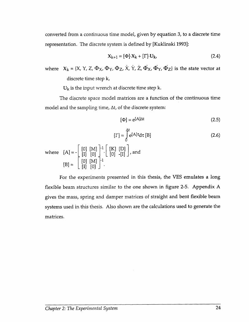
converted from a continuous time model, given by equation 3, to a discrete time

representation. The discrete system is defined by [Kuklinski 1993]:

Xk+1 = []'-Xk + [F].Uk, (2.4)

where Xk = {X, Y, Z, 'Ix, (IY, (Dz, X, Y, Z, Ojx, (Y, (Iz} is the state vector at

discrete time step k,

Uk is the input wrench at discrete time step k.

The discrete space model matrices are a function of the continuous time

model and the sampling time, At, of the discrete system:

[D] = e[A]At (2.5)

[F] = Ae[]Adt [B] (2.6)

where [ [0] [M] -I [K] [D] adwhere [A]= - [I] [0] [0] -[I], and

[B]= [[0] [M] -1

;[B] = [I] [0]

For the experiments presented in this thesis, the VES emulates a long

flexible beam structures similar to the one shown in figure 2-5. Appendix A

gives the mass, spring and damper matrices of straight and bent flexible beam

systems used in this thesis. Also shown are the calculations used to generate the

matrices.


Flexible SuDoortinaStructure T i

Inertial Reference Frame

Figure 2-5: Typical VES Space Robotic SystemFigure based on [Torres 1993]

2.4 The VES Control Architecture

The VES system is controlled by a fairly complex arrangement of

computers and controllers. In addition, performing micro-gravity emulation

experiments requires the user to coordinate two control computers.

2.4.1 An Overview

Figure 2-6 summarizes the VES computer architecture. A Sun

Workstation serves as the primary interface and software editing platform. The

Sun is connected to the main control system via Ethernet.

Admittance based control of the VES platform is supervised by the

Redslave, a 68030 based single board computer running the vxWorks operating

system. Admittance control is performed using the force sensor measurements

read from an analog to digital converter. The desired platform position is

converted to individual actuator lengths by inverse kinematics. The Redslave


Sun Workstation

Figure 2-6: VES Computer Architecture

sends the desired lengths to individual legslave controllers through a custom

made leghost card at around 100Hz.

The legslaves perform closed loop proportional-derivative control at

500Hz to maintain the desired lengths. The legslaves control the actuator lengths

with a signal to Servo Amp cards which send a controlling current to the

corresponding servovalve at 1000Hz. A Temposonics linear transducer in each

leg sends an electromagnetic pulse from the base of the leg through a shaft

inside the rod which is reflected back at the end of the leg. The time it takes for

the pulse to return is measured by a Temposonics card and made available to the

legslave every 341 milliseconds. This provides an accurate leg length as feedback

for the closed loop controllers. The legslaves also filter the feedback signals to

prevent exciting the natural vibrational modes of the hydraulic legs [see Chapter

5].


The control of the robotic system mounted to the platform is distinct from

the control of the platform. The Blueslave, a 68020 based single board computer

running the vxWorks operating system, supervises the control of the robotic

system. In this thesis, a PUMA 560 was the only robotic system used with the

VES. The Blueslave sends desired joint positions to and receives actual joint

encoder signals from the PUMA through a Programmable Multi-Axis Controller,

or PMAC. The PMAC can perform PID control on up to 8 joints at a time.

When micro-gravity emulation is performed, coordination is required

between the platform control system (Redslave) and the robotic control system

(Blueslave). The Redslave makes information about the inertial orientation of

the platform top available to the Blueslave. In the Model Method, the Blueslave

uses this information to calculate an estimate of the gravitational wrench and

provides that information to the Redslave so it can be subtracted from the force

sensor measurements per Equation 2.1. This transfer of information is done

through a shared memory space on the Redslave which both the Redslave and

Blueslave can access.

2.4.2 The Platform Admittance Control Cycle

Before an admittance model experiment begins, with or without micro-

gravity emulation, a sample rate and admittance model type must be selected.

The main platform control loop is driven by a clock interrupt. The sample rate

specifies how often the interrupt will be given. If the interrupt comes before the

admittance control cycle has been completed the experiment is halted. Sample

rates are generally in the range of 75Hz-90Hz, and depend on the number of

safety routines activated and the type of admittance model being used. If a

complex coupled admittance model is being used, then every element of the 6 by

6 [D] and [r] matrices (see Section 2.3) must be used in the admittance


calculations. If the admittance model is linearly decoupled, then only the

diagonal terms are necessary. Similarly, if the admittance model is of a beam,

then only certain terms, about half, might be used in the calculation. For a given

admittance model, then, the most computationally efficient calculation method is

adopted.

Figure 2-8 summarizes the basic admittance control cycle which the

Redslave performs during an experiment. The clock interrupt starts the cycle.

First, the forces are read from the force sensor. If micro-gravity emulation is

being performed, then a gravity wrench estimate from the Blueslave is

subtracted from the measured value. Next, the admittance controller performs

the calculations described is Section 2.3 to determine the desired position and

velocity of the platform. Inverse kinematics are then performed to turn these

values into individual leg lengths. A series of safety calculations are then

performed to be sure that the desired leg lengths fall within pre-defined safety

margins. Finally, the desired leg lengths are sent to the individual legslave

Figure 2-8: Admittance Control Cycle

Chapter 2: The Experimental Systenm

Figure 2-8: Admittance Control Cycle

controllers. More detail of the control software is presented by [Kuklinski 1993].

2.4.3 PUMA 560 Control

The Blueslave controls the motion of the PUMA 560. Direct control of the

PUMA is performed by the PMAC. Communication between the PMAC and

Blueslave is made simple with the use of dual-ported ram (DPRAM), a memory

location which is accessible from both computers. For real time control, the

PMAC receives position commands and provides joint encoder information

through DPRAM, but this communication is not automatic. The PMAC is

programmed to continually read from and/or provide information to a DPRAM

address. This small sub-program internal to the PMAC is called a PLC. For real

time motion control, a Motion Control Program is written on the PMAC to read

desired joint positions and velocities from a buffer space. The buffer space

allows the PMAC to always make a smooth transition between any two

commanded positions. The PMAC always looks two commands ahead for this

reason, so a sufficiently large buffer space is required to allow the Blueslave to fill

it with commands while the PMAC is busy performing those commands.

Software has also been written for the Blueslave to estimate the

gravitational wrench for the robotic system it is controlling. The theory and

form of these equations is presented in Chapter 3. A series of calibration and

zeroing procedures are required to accurately perform micro-gravity emulation.

A detailed guide to these procedures is presented in Appendix E. Details of the

PUMA/PMAC interface and DPRAM are presented by [Baker 1992].


2.5 Summary

This chapter described the basic components and operation of the VES II,

including the control architecture and the PUMA 560.

admittance control concept was also presented.

The basic theory of the


Chapter 3

Emulating Micro-Gravity

3.1 Introduction

This chapter presents the analytical basis which allows gravity to be

compensated for to emulate micro-gravity. In Section 3.2, the inherent difficulty

in estimating the effects of gravity is discussed, the sources of estimation error

are presented, and limits are set for these errors.

The Learning Method and the Model Method are then presented in

Sections 3.3 and 3.4 to compensate for gravity and emulate micro-gravity using

the VES. The Model Method uses a mass parameter model of the manipulator to

calculate and compensate for the forces and moments caused by gravity. The

Learning Method uses an iterative learning approach which avoids the need for

careful, detailed parameter estimation. Experimental results are presented which

show that these methods can accurately extract even relatively small dynamic

interactive behaviors from much larger gravitational effects. The two methods

are compared in Section 3.5. Note that these methods do not remove the gravity

forces seen by manipulator joints, they predict the gravitational wrench at the

base of the robot. If necessary, however, joint balancing or feedforward

Chapter 3: Emulating Micro-Gravity

computed torque-control techniques can be used to remove the effects of gravity

on the joints.

3.2 The Challenges of Micro-Gravity Emulation

The basic concept of these micro-gravity emulation methods is to subtract

the gravity wrench seen by the force sensor from the total wrench to yield an

estimate of the dynamic wrench. Micro-gravity emulation can be difficult to

achieve if the dynamic wrench estimate is corrupted because of inaccurate

estimates of the gravity wrench. Even small errors in the dynamic wrench

estimate can cause large errors in the motion of the system.

3.2.1 _ Wrench Error Sensitivity

The sensitivity of dynamic wrench estimates to gravity wrench errors can

be easily demonstrated experimentally. A flexible beam similar to the one

shown in Figure 2-5, described in Section A.3, with a PUMA 560 on it was

emulated with the VES system. The PUMA was commanded to move its

shoulder joint, ql, through 180 degrees of motion in 2 seconds with its arm and

forearm extended perpendicular to the q1 axis as shown in Section A.5. This

created a large dynamic wrench shown by the solid line in Figure 3-1. Also

shown in Figure 3-1 is the range of dynamic wrench estimates, Td, which will

result if the error in the gravity estimate, 6Tg, is bounded by 1% or 5% of the

total gravity wrench. Clearly, even small errors in Vkg will badly corrupt an

estimate of kTd since Wg, the gravitational wrench, is much larger than Wd. It is

also clear that small sensor errors create similarly large errors in kd, since it

must measure the large true gravity wrench. The basic problem is that the

sensor must measure a large force (about 1000 Newtons) with very high

accuracy.


100

80600z

w 400

U 20

,• 0

0-20-40

E 50-zE 40-0Z. 30-0

S20-

~ 10-0

0 4 8 Time (sec) 16a. Forces

I I I I0 4 8 Time (sec) 16b. MomentsFigure 3-1: Dynamic Wrench Vectors with Gravity Error Ranges

3.2.2 Position Error Sensitivity

The above problem is compounded by the fact that even small wrencherrors can cause large position errors during micro-gravity emulation for manyspace systems. For example, Figure 3-2 shows the translation of the manipulatorbase in the Zi direction, defined in Figure 2-5, during the experimental micro-gravity motion described above. The base motion is shown with 0%, 0.5% and1% errors in the gravity wrench estimate. Even a 0.5% wrench error causes avery different motion compared to the case with no error, resulting in a pooremulation. For many admittance models, force errors of as little as 1% willactually cause motion errors which are several times the size of the true micro-gravity motion of the system.


_ ~_ _

I -I

0.00

-0.05

N

0 -0.10

O -0.15

> -0.20

0 2 4 6 8 10

Time (sec)Figure 3-2: Micro-Gravity Motions with Ag Errors

3.2.3 Required Estimation Accuracy

A simulation of a typical space robotic system was constructed to

investigate the sensitivity of the emulations to gravity wrench estimation errors.

Errors were introduced to the dynamic wrench of the simulations and the effect

on the system motion was observed. It was found that to maintain motion

accuracy of a few percent, it was necessary for the errors in AVd, called WAd, to be

less than 1.0 Newton of force or 1.5 Newton-meters of moment for the VES with

a typical payload of a thousand Newtons. The gravity wrench estimate must

therefore be accurate to 0.1%, which is no easy task.

3.2.4 Error Sources

Error in the dynamic wrench estimate has two main sources, the sensor

measurement error, 6Ws, and error in the gravity wrench prediction, d6yg = Wg

- g g. The total dynamic wrench estimate error is their sum:


W&d = Ws + W g, (3.1)

Both these error sources must be minimized to emulate micro-gravity

accurately.

Some errors in sensor measurements are repeatable. For example the

geometry of strain gauges used in the sensor causes a signal in one axis because

of forces in another. This "cross talk" is a repeatable sensor error. The

electronics which process the strain gauge signals can also introduce repeatable

errors. Multiplying the signals by a calibrating matrix was found to compensate

effectively for these repeatable errors since our sensor and electronics are well

characterized by a linear model. A method of experimentally determining this

calibration matrix is presented in Section 3.4.5.

Non-repeatable sensor errors occur principally due to high frequency

electronic noise ( > 10-20 Hz) and low frequency thermal drift (< 1 Hz). High

frequency noise can be eliminated by analog and digital filters. Note that only

relatively low frequency signals are necessary for micro-gravity emulation.

Signal frequencies well above the natural frequency of the space system being

emulated, generally a few Hertz, can be filtered. The effect of low frequency

drift can be minimized by establishing a protocol to reset the sensor offsets

before each experiment. Details of the force sensor noise and drift are presented

in Section 5.2.1.

Although system performance during micro-gravity emulation is very

sensitive to sensor errors, we found that these could be reduced to acceptable

levels by the use of a high quality sensor, precise multi-axis calibration, filtering,

and careful experimental protocols. The reduction of the other major error

source, the gravity wrench estimate, is not quite so direct.

The gravity wrench is a function of several variables:


Wg = Wg(q,D,P), (3.2)

where q is a vector of the manipulator system joint displacements, (D is a 3x1

vector of manipulator base (Stewart platform top) inertial orientation angles, and

P is a vector of mass parameters of the system.

Both q and D are controlled variables, while P is a physical property of the

manipulator. Each of these variables can introduce some error to the gravity

wrench estimate. The gravity wrench due to manipulator joint errors are not

generally important. Typical manipulator joint encoders produce such small

errors that they have a negligible effect on 86Tg. Although errors in knowledge

of the manipulator base orientation can cause significant errors in the gravity

prediction, the positioning accuracy of the VES Stewart platform can be used to

greatly reduce these errors (see Section 5.2.2). The major source of error in Ag

is reduced to the term, P, in Equation 3.2.

Two methods are presented for accurately predicting the gravitational

wrench, the Learning Method and the Model Method. The Model Method

directly finds the manipulator mass parameters, P, and the exact relationship of

Equation 3-2, while the Learning Method iteratively finds Wg without explicitly

solving for the mass parameters.

3.3 Learning Method Gravity Compensation

The gravitational wrench of a manipulator can be "learned" iteratively

during its motion on the VES. This produces accurate space emulations with

minimal analysis and real time computation. Also, it does not require accurate

mass parameter identification. However, the learning method can be used only

for experiments where the commands to the system are known in advance and


are repeatable. It is inapplicable for telerobotic experiments involving human

supervisors, or for other experiments with spontaneous events.

The method finds directly the reaction motions of the manipulator base

structure (the platform top) caused by the dynamic forces for a given

manipulator motion, q(t). At each iteration, a trajectory of the manipulator base

9(t), an approximation of the micro-gravity dynamic base motion, is used to

form an estimate of the gravity wrench Wg(t). The manipulator is moved very

slowly through q(t) while its base is moved through ý(t) and the sensor readings

are recorded. Since the gravity wrench is a function only of system positions, at

low velocities (those with negligible dynamic effects) the measured wrench will

be equal to the gravity wrench. The accuracy of this estimate depends on how

closely the base motions used in the iteration approximate the true micro-gravity

dynamic motions. If the true micro-gravity base motion is not large, an initial

guess of no base motion can be iteratively improved until the correct micro-

gravity system motion is found. The estimate found, 1g, is then subtracted

from actual sensor readings during a full speed motion to yield an estimate of

the dynamic base wrench, kd, which is then used by the controller to produce a

better estimate of the micro-gravity base motion. Hence the iterative procedure

consists of obtaining an improved estimate for the platform motion and then

using the platform motion to produce an improved estimate of Wg.

3.3.1 The Learning Algorithm

The iterative learning procedure can be written as follows. First we

define:

s = x -t is a time variable scaled by ox,

q(s) is a well defined, repeatable manipulator motion,

g(s) is a gravity wrench estimate for iteration i, and


Y'(s) is an estimate for the trajectory of the manipulator base in

iteration i.

First, the admittance model of the spacecraft or supporting structure to be

emulated is developed and programmed into the VES. Figure 3-3 summarizes

the two phase iterative procedure. At each iterative step i {i=1, 2, ... n} the

following occurs:

PHASE A:

1) The time scale is set to make all actions slow, with no dynamic effects,

0c)x1.

2) The platform performs motion estimate Qi-l(s) slowly, while the

manipulator moves slowly through q(s). Recall that the initial guess

%O(s) is usually no motion.

3) The wrench on the sensor is recorded as an estimate for the gravity

wrench & g(s), with no dynamic effects

PHASE B:

4) The time scale is set to create full speed actions, ao=1, and the

manipulator moves through q(s) at full speed.

5) A dynamic wrench estimate is formed by subtracting the gravity

wrench estimate (recorded in step 3) from current sensor

measurements: dZa(s) = Ws -V (s).

6) AT/(s) is used as input to the admittance model, which moves the

platform through •i(s), an improved estimate of the actual micro-

gravity platform motion.

7) Iteration i+1 begins at step 1.


PHASE A: Slow speed motion, System Under Position Control

Input: Y(s). Wg is recorded

q(s)

(s) physical WgY(s) systemr--m--------

F-PHASE B: Full speed motion, System Under Admittance Control

A

Input: Wg. Y(s) is recorded

Sg-If l [

I -

L

Figure 3-3: Learning Algorithm Schematic

If the method converges, it can be shown that the final dynamic wrench

d(S ) and base motion ('n(s) correspond to micro-gravity conditions. Successive

base motion estimates will generally converge quickly to some accuracy.

Substantial dynamic wrench errors may result in the platform trying to move

outside its workspace when there are large errors in the initial base motion

guess. In these cases the VES safety systems will abort the procedure.

This iterative method is similar to a method used to learn all the static and

dynamic mass parameters of a manipulator to improve the accuracy of

manipulator motions [Arimoto et. al. 1984]. The convergence characteristics of

the Learning Method are also similar to the method presented by Arimoto.

The following subtleties also apply to the Learning Method. First, the

motion of the manipulator does not have to be known accurately: only the

commands to the manipulator must be known and repeatable. The actual micro-


gravity motion of the manipulator joints will converge along with the base

motion. Second, for some cases, the initial guess of no base motion may be

replaced by some other trajectory, say one based on simulations.

3.3.2 Emulation Accuracy

The Learning Method was used to emulate micro-gravity on the VES.

Once again, the system idealized in Figure 2-5 and described in Section A.2 was

emulated with a PUMA 560 mounted on the VES. The PUMA was commanded

to move its arm through the same 180 degrees of motion during repeated

iterations of the learning method. After nine iterations of the learning algorithm

the micro-gravity motions of the manipulator base converged to less than a

millimeter, or less than .001 radians in each axis. The convergence of the motion

in successive iterations for rotations about the Xi axis and the Zi axis of the

manipulator base is shown in Figure 3-4.


0.03

0.02

x 0.01

" 0.00o

0 -0.01

0 -0.02

-0.03

0 2 4 6 8 10Time (sec)

S0.010

, 0.005

0.0000 o.ooo

o -0.005

-0.010

0 2 4 6 8 10

Time (sec)

Figure 3-4: Rotation of Base During Learning Iterations

3.4 Model Method Gravity Compensation

The model based method analytically formulates the wrench due to

gravity at the base of a manipulator, which is uniquely determined by its mass

parameters, joint angles and base orientation. The basic analytical formulation

was proposed by [West et. al 1989], with no experimental results. The method

presented here requires experimentally finding the manipulator mass


parameters very accurately. With the analytical relationship and the mass

parameters, Wg can be calculated, allowing the VES to compensate for gravity

and emulate micro-gravity without a priori knowledge of the system inputs.

This permits studies such as telerobotic experimentation or human supervisory

control.

3.4.1 Determining Mass Parameters

Mass parameter identification is the key to accurately predicting the force

and moment at the base of a manipulator due to gravity. Several algorithms

have been developed to experimentally determine the mass and inertial

parameters of manipulators [Mayeda et al. 1984, Olsen et al. 1985, Mayeda et al.

1988]. These methods use motor torque information to solve for the dynamic

parameters, which are generally used in feed forward or computed torque

control of the joints. These methods are limited to manipulators with low joint

friction, such as direct drive. Regardless, many of the parameters found are not

required for space emulation, and the lowest, undriven, link is not modeled.

Mass parameters can be found by disassembly and measurement of the

manipulator [Armstrong et al. 1986]. This method is tedious, and does not

account for variations in the manipulator.

A method of experimentally determining mass parameters of a

manipulator is presented. The parameters found are used to predict gravity

forces and moments exerted at the base of the manipulator. Experimentally

finding the mass parameters of the manipulator allows an arbitrary manipulator

to be quickly modeled and then used in an emulation.


3.4.2 Formulating the Model

The analysis that follows is presented for a single serial link manipulator

system whose base is capable of being positioned accurately in inertial space.

The geometry and Denavit-Hartenburg parameters of a PUMA 560 are

presented in Appendix B, and the development of this mass parameter analysis

for the PUMA 560 is presented in Appendix C.

Consider a stationary general manipulator with n links oriented

arbitrarily in inertial space in order to develop a model of manipulator mass

parameters. Applying elementary laws of statics, the gravitational wrench at the

base of the general manipulator can be written:

1Fg = j(mi){bg}1 = (Mt 0ota){b (3.3a)g n= Xbrlx {g}mj) (3.3b)

where mi is the mass of link "i", bg is the gravitational force vector transformed

to the coordinate frame of the manipulator base, and bri is the position vector to

the ith link's center of mass from the manipulator base coordinate frame,

expressed in the manipulator base frame.

The inertial orientation of the base of the manipulator is defined by the Z-

Y-X constant angle (roll-pitch-yaw) convention [Craig 1989]. The transformation

matrix for this convention can be used to write the gravitational force vector in

the manipulator base frame as:gx 0

b = gy =[Txyz ]T =gz -g

(3.4)

where Ox, Oy and Oz are the roll, pitch, and yaw of the manipulator base in the

inertial frame, shown in Figure 2-4. The manipulator base is mounted accurately

on the top of the VES platform in our experimental system; hence the


manipulator base inertial orientation is known by the VES system. The mass

parameter constants, mi and bri for each link, are not known.

The manipulator model and the method for experimentally finding the

model are based on Equations 3.3 and 3.4. The model has two parts; one for

predicting gravity forces, Equation 3.3a, and one for moments, Equation 3.3b.

3.4.3 Estimating Gravity Forces

Estimating the gravity forces at the base of the manipulator requires

finding the total mass of the manipulator, Mtotal, and using Equation 3.3a. An

estimate for Mtotal could be formed from one force sensor measurement at a

known platform orientation, essentially weighing the manipulator.

Unfortunately, small errors in the sensor or orientation could lead to large errors

in subsequent force predictions by this method. A better approach is to average

out the effects of small random errors. A large sample of m force

measurements is collected at various orientations and the corresponding

gravitational accelerations are calculated by Equation 3.4. A minimization of the

errors can then be achieved in a fashion similar to the pseudo-inverse or least

squares approaches. Individual estimates for Mtotal are weighted by their

magnitudes and averaged, producing a best estimate for Mtotal according to:

Mtotal = T (3.5)S{bjT b• (

where b=[bg(l)}T bg( 2 )T ... {bg(m)T] is a vector composed of m

gravity force vectors in the manipulator base frame, and

F = Fs(1)T Fs(2 ) ... Fs(m)T is a vector composed of the m sensor

force vector measurements.


The Mtotal found is the only model parameter needed to predict the forces

due to gravity.

3.4.4 Estimating Gravity Moments

The position vector of each link's center of mass in that link's coordinate

frame, ri, is a mass parameter constant of the manipulator. The position vector

to each link's center of mass from the manipulator base frame, bri, can be found

with a transformation matrix:

bri = [A] - ri (3.6)

This transformation is shown for joint two of a PUMA 560 in Figure 3-5.

Note that both bg and [bA] are configuration dependent (knowns) while rij and

mi are the mass parameter constants of the manipulator (unknowns).

Figure 3-5: Link "i" center of mass vector

The transformation of Equation 3.6 can be used to rewrite Equation 3.3b,

the moment at the manipulator base caused by gravity:

1 0 0 0 rixMMg= 0 1 0 0 A .riy

i=0 0 0 1 0 riz

bgx

x (mi) . ,b gy'b~z'

(3.7)


where {rix riy riz}T is the position vector for the link "i" center of mass in the link

"i" coordinate frame, and

[ A] is the homogeneous transformation matrix from the ith link frame

back to the manipulator base frame.

Equation 3.7 can be expanded to produce three equations for the gravity

moment (for the three axes) with 4n+1 terms in each of the three axes. Recall

that n is the number of links. This calculation is shown for the PUMA 560 in

Appendix C. The constant mass parameter terms (mo0rox, m0oroy...) can be

factored out as a 3(n+1) by 1 vector, Q, leaving the equation in a simplified linear

matrix form:

Mg = [W(q,)] {(Q}. (3.8)

where the matrix [W(q,(D)] is a function of joint angles and manipulator base

orientations of dimension 3 by 3(n+1).

Matrix [W] is a function of the inputs, while Q is a function of the constant

mass properties. Expressions for both [W] and Q for a PUMA 560 are shown if

Appendix C. Physically, each term in Q represents a link mass times a moment

arm for some link axis, such as 'ml'rlz'. Link lengths and offsets produce an

extra term in the elements of Q which are aligned with the offset or link length,

such as 'm2"r2z + (m2+m 3)-d2 '. The base of the manipulator is treated as an extra

link since it has mass which is offset from the ideal manipulator base, causing

some moment.

The columns of [W] contain gravity acceleration components which

combine with a "mass times moment arm" element from Q to produce the

gravitational moment. Since each revolute joint axis is defined in space by only

two angles, one of the three columns added to [W] for that link will be

proportional to a previous column, or identical for orthogonal joints. In other


words, the gravity acceleration component for one axis of each link will be

aligned with an axis from the previous link. Prismatic joints will have two axes

similarly aligned. This alignment causes identical acceleration components which

appear as linearly dependent columns in the [W] matrix. Subtracting dependent

columns produces:Mg = [G(q,/)] P)}. (3.9)

where [G(q,D)] is a new configuration dependent matrix of dimension 3 by 3

+2(# revolute joints) + (# prismatic joints), and P is a mass parameter vector of

matching dimension.

The vector P is the model of the manipulator necessary for predicting

gravitational moments. Although each element of P contains several constants,

only their sum is required, producing a simplified model of the manipulator .

Equation 3.9 could be solved for P by collecting a minimal set of

independent [G] matrices and Mg vectors to create a linear set of equal

equations and unknowns. This method produces poor results, since it is very

sensitive to small errors as we found in estimating forces. A better approach is

the least squares solution. The vector which minimizes the squared error

I[A]{x} - {b} 2 for the linear equation [A]{x} = {b} is:

Xbest = [A] [A]]-I[A]T{b}, (3.10)

where the [[A]T[A]] matrix is invertible if and only if [A] has independent

columns. The least squares approach allows a large data sample to minimize the

errors over the entire equation range.

Since our geometry dependent matrix [G] has independent columns, we

can compose a least squares solution in the form of Equation 3.10. We calculate

[G(i)] matrices at m unique configurations and combine them to form:


[G] = [[G(1)]T [G(2 )]T

The m corresponding sensor moment vector measurements are combined

producing:

M= [M(1)T M(2)T ... M(m )T] .

We then solve:

P =

(3.12)

(3.13)

where P is the best estimate of a model which can be used to predict gravity

moments by Equation 3.9.

Together, estimates of P and Mtotai form the minimal model parameters

required to predict the forces and moments due to gravity at the base of a

manipulator.

3.4.5 From Theory to Application

The preceding analysis suggested a procedure for estimating the mass

parameters, P and Mtotal, which could then be used to estimate the gravitational

forces and moments by Equations 3.3a and 3.9. Unfortunately, achieving

experimental results which met the strict requirements of Section 3.2.3 was more

difficult.

Analysis revealed that the experimental estimation procedure was very

sensitive to errors in the force sensor calibration matrix. The calibration matrix

converts the signal from the force sensor into actual force and moment readings

in SI units:

SWapp = [C] Wsig,


(3.14)

(3.11)... [G (m)]T T .

where SWapp is the wrench (in SI units) applied to the force sensor in the sensor

frame (Appendix D defines the sensor frame and conversion to the

platform top frame),

Wsig is the wrench signal read from the strain gauge attenuation

circuitry via the analog to digital converter, and

[C] is the calibration matrix.

An estimate of the calibration matrix can be constructed from the

manufacturers data and a measurement of the gains of the strain gauge

amplifiers. Unfortunately, the accuracy of the manufacturers estimate is

unknown and the procedure for measuring the amplifier gains is not very

accurate. A discussion of the calculation of this matrix can be found in [Baker

1992] and [Kuklinski 1993].

A method was devised for determining the calibration matrix

experimentally in a manner similar to the mass parameter estimation routine. If

the manufacturer's estimate of the calibration matrix is reasonably good, then

the mass parameter estimation of Equation 3.13 should prove equally good.

Equations 3.5 and 3.13 can then be used to estimate the gravitational wrench.

This wrench estimate can be used for SWapp in Equation 3.14. An experimental

estimate of the calibration matrix can then be found by combining six wrench

estimates, SWapp, and six signals from the sensor, Wsig, and solving Equation

3.14. Once again, a least squares approach with a large sample of data across the

entire workspace of the platform and manipulator will produce the best result.

The platform and manipulator are commanded to "m" different

configurations. At each configuration "j", Equations 3.5 and 3.13 produce an

estimate of the applied wrench, SWapp(j). These are combined to form:

[i app] : [Wapp(1) Wapp( 2 ) ... Wapp(m)]. (3.15)


Similarly, at each configuration "j" the signals from the force sensor are also

recorded and combined, making:

[Wsig] = [Wsig(1) Wsig( 2) ... Wsig(m)]. (3.16)

A least squares solution can then be written:

[C]= Wapp ] Ws .[ sig] Wsig . (3.17)

By alternately re-estimating the calibration matrix and the mass

parameters, it was found that they converged quickly to within some range.

Unfortunately, this still resulted in several Newtons or Newton-meters of error

which was unacceptable.

Experimentation showed that the range of the wrench convergence was

roughly equal to wrench errors due to inaccuracies in the knowledge of the

platform position. The original procedure was to command the platform to a

position and then freeze it. It was assumed that the platform accurately

maintained its position. Gravity estimation, however, is very sensitive to the

base orientation of the manipulator, so even errors of half a degree were

unacceptable. This problem was solved by improving the coordination between

the two control computers to allow the platform to remain under position

control while the wrench measurements were made.

When the platform position was known accurately, the iterative process

of estimating a calibration matrix and mass parameters was repeated. This time

the errors in gravity force prediction were reduced much farther, very close to

the range of errors found in the force sensor itself. Some improvement was

made in the noise errors of the force sensor (see Appendix F) yet it remains the

dominating source of error in accurate gravity compensation.


3.4.6 Emulation Accuracy

The first step in emulating a gravity free system is to model the

manipulator. Estimates for Mtotal and the P vector were found for a PUMA 560

by the method described above. The manipulator and VES platform were

moved through a series of 47 positions. in each configuration "j": a geometry

matrix [G(j)] was calculated from the measured platform orientation and robot

position, a gravity vector bg(j) was formed from orientation information, and

measurements Fs(j) and M(j) were collected. The data from all configurations

was combined to form a [G] matrix, a bg vector, an M vector, and an Fs vector

as described above. A manipulator model was then formed by solving

Equations 3.5 and 3.13 for Mtotal and P.

The mass parameter estimates found were then used to find an improved

estimate for the calibration matrix. The system was commanded through the

same series of 47 positions. Vectors of SWapp(j) and SWsig(j) were collected at

each position "j". These were combined to form the matrices [Wsig] and

l[iapp]. A best estimate for [C] was then generated from Equation 3.16.

After two iterations of this procedure, estimates of the gravitational

wrench were accurate to within the required range. Further iterations did not

significantly improve the accuracy, although the values for the mass parameter

estimate and [C] changed by a few percent. The mass parameter estimates

found in this way were similar to physical mass parameter measurements, see

Section C.3.

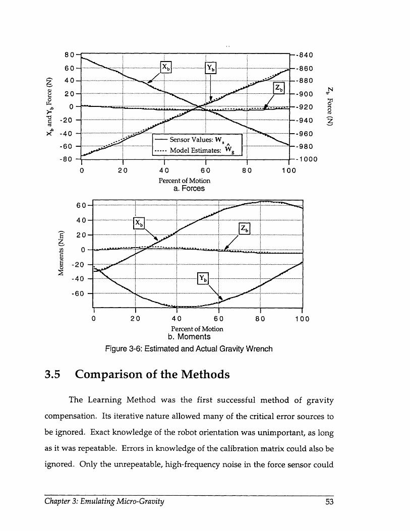
To check the accuracy of the gravity wrench estimates, the model was

used to predict gravity wrenches over the range of motion of the system. This

predicted value, and the actual sensor readings were collected for several very

slow movements of the manipulator and the base which had negligible dynamic


effect. The manipulator moved joint 1 through the 180 degree rotation described

earlier, while the platform was commanded to rotate the manipulator base from

+5 degrees to -5 degrees rotation about the inertial X and Y axes. Table 3-1

summarizes the error in •Tg, the difference between estimated and measured

values, showing the average and maximum error found in each axis. Figure 3-6

shows the measured and estimated wrenches over the entire motion. The

accuracy of •Tg found with this experimentally identified robot model met the

goal set in our sensitivity analysis

TABLE 3-1: Errors in Gravity Prediction


Axis RMS. Error Max. Error

Xb Force 0.46 N 0.95 N

Yb Force 0.24 N 0.53 N

Zb Force 0.46 N 1.4 N

Xb Moment 0.62 Nm 1.14 Nm

Yb Moment 1.01 Nm 1.67 Nm

Zb Moment 0.06 Nm 0.13 Nm

80

60

40

20

0

-20

-40

-60

-80

20

60-

40-

20-

0-

-20 -

-40 -

-60 -

40 60Percent of Motion

a. Forces

880

I I I I20 40 60 80

Percent of Motionb. Moments

Figure 3-6: Estimated and Actual Gravity Wrench

I100

100

3.5 Comparison of the Methods

The Learning Method was the first successful method of gravity

compensation. Its iterative nature allowed many of the critical error sources to

be ignored. Exact knowledge of the robot orientation was unimportant, as long

as it was repeatable. Errors in knowledge of the calibration matrix could also be

ignored. Only the unrepeatable, high-frequency noise in the force sensor could


- Sensor Values: W,

-- Model Estimates: Wg

I.............................. ............. .............. ....... ..................................

*__.. .......................

. . _..

.. ..... ..... .. .. ...... ..... ....

:·-------------- ......--........................ ........ .... ... ........ ............ .. ...... ........ ......

-840

-860

-880

-900

-920

-940

-960

-980

-1000

............... ... .. .. .. .. ...... .. ... ... ... ..

, .. ...................... ............................ .........1...................................

.. ............ ............ ........ ..... ... ......... ...........

i

not be overcome with the Learning Method. Although the Learning Method has

a good accuracy and is computationally very inexpensive, it takes quite a bit of

time to perform an experiment. Each experiment must be run through several

iterations, and half of those iterations are at a very slow, non-dynamic, speed

which is generally 1/20th the normal speed. This means that a 20 second

experiment can take over 20 minutes to perform just once. Even though the

Learning Method could be used to emulate micro-gravity, there was still a need

for a more practical, faster method of emulation, in addition to the need to

emulate experiments without pre-planned motions.

The basic idea behind Model Method was proposed in 1989 [West et al.

1989]. The most challenging aspect of this method was not theoretical, it was in

the application. Accurate knowledge of the robot orientation was very

important, as was reduction of the force sensor errors. The final improvement

which allowed this method to achieve the high accuracy desired was the

estimation of the calibration matrix described in Section 3.4.5.

Figure 3-7 shows the gravity compensated dynamic moment in the Xb

axis for an experiment performed with both the Learning Method and the Model

Method. Figure 3-8 shows the close correlation in the base motion produced by

the two methods. Both of these methods have been used successfully to verify

the effectiveness of path-planning and control algorithms for space robotics in a

number of studies, see Chapter 4.


40

20

0

-20

c -40

0 2 4 6 8 10Time (sec)

Figure 3-7: Micro-Gravity Moment

0.03

' 0.02

x< 0.01

0-o

-0.01

0 -0.02

-0.03

0 2 4 6 8 10Time (sec)

Figure 3-8: Micro-Gravity Rotation

3.6 Summary

This chapter presented the theoretical developments for gravity

compensation. The difficulties of estimating the effects of gravity were

discussed. Then, two methods were presented to compensate for gravity on the

VES II, the Learning Method and the Model Method. Experimental results were

presented which showed that these methods can extract even small dynamic


forces from the larger gravitational effects to accurately emulate a micro-gravity

environment.


Chapter 4

Investigation of Planning and Control

Methods

4.1 Introduction

The high cost of space operations and the dangers involved in manned

space operations has created a heightened interest in the field of space robotics.

Many control theories and manipulator path planning algorithms have been

proposed to improve the speed and accuracy of robotic space operations

[Papadopoulos and Dubowsky 1993, Xu and Kanade 1993]. The VES system

described in the preceding chapters has been used to investigate several of these

algorithms experimentally.

A series of algorithms were investigated which deal with one of the

fundamental problems of space robotics. A common scenario in space robotics

will be the maneuvering of a small dexterous manipulator whose gross

positioning is achieved by a less accurate long flexible manipulator, such as the

proposed space station scheme the SSRMS. The main problem is the accurate

positioning of the small dexterous manipulator. Motions of the small

manipulator will excite the low frequency vibrations in the long flexible

Chapter 4: Investigating Space Robotics Theories

manipulator, causing the small manipulator to bounce around. In this study, the

long flexible manipulator, the base of the dexterous manipulator, is assumed to

be a simple flexible beam system.

Two basic algorithms which deal with this vibration problem are

investigated. One algorithm, the Coupling Map, is used to minimize the amount

of vibration caused during a motion [Torres and Dubowsky 1993]. A second

algorithm, called Pseudo-Passive Energy Dissipation (PPED), is used to remove

the vibrations once they are caused [Torres 1993]. A third algorithm, which is

not presented here, such as Coordinated Jacobian Transpose Control [Sunada

1994] could be used to maintain the end effector in an accurate position despite

any vibrations which remain.

4.2 The Coupling Map

A path planning algorithm for a manipulator mounted on a compliant

base in zero gravity was proposed by [Torres 1993, Torres and Dubowsky 1993].

The coupling map is a tool for finding paths in manipulator joint space which

minimize the energy transferred into the compliant base during manipulator

motions. Energy transferred to the base causes motion which damp out very

slowly, increasing the duration and expense of space operations. This approach

would be used to plan the motions of future space robotics systems. The

coupling map theory has produced good results in simulation and planar

experiments [Torres 1993, Torres and Dubowsky 1993], and is experimentally

verified in full spatial motion here.

The coupling map is a function of the compliance and damping

characteristics of the base (the long reaching flexible manipulator) as well as the

static and dynamic parameters of a manipulator with n joints. Analysis of the

system equations of motion with the assumption of small motions and wrenches


produces the coupling matrix [Torres 1993]. The coupling matrix, [Q(q)], is a

measure of the sensitivity of the support structure to receiving strain energy

from the manipulator in a given manipulator configuration. The eigenvectors of

[Q(q)] suggest joint motion directions of maximum and minimum energy

transfer at location q in joint space. Lines of minimum energy transfer can be

drawn in joint space by following the minimum eigenvectors; the magnitude of

the eigenvector is represented by the darkness of the line. These lines can be

easily visualized for a 2 degree of freedom system with a coupling map of

minimum energy lines. Higher degree of freedom systems are more difficult to

represent visually, cross sectional coupling maps can be drawn for any two joints

by fixing all others. The disturbance of the base for any manipulator path is

shown by the darkness of the lines crossed in the map. Traveling parallel to a

line transfers the minimum possible energy to the base in that region. Darker

regions are called high coupling areas while lighter regions are low coupling

areas.

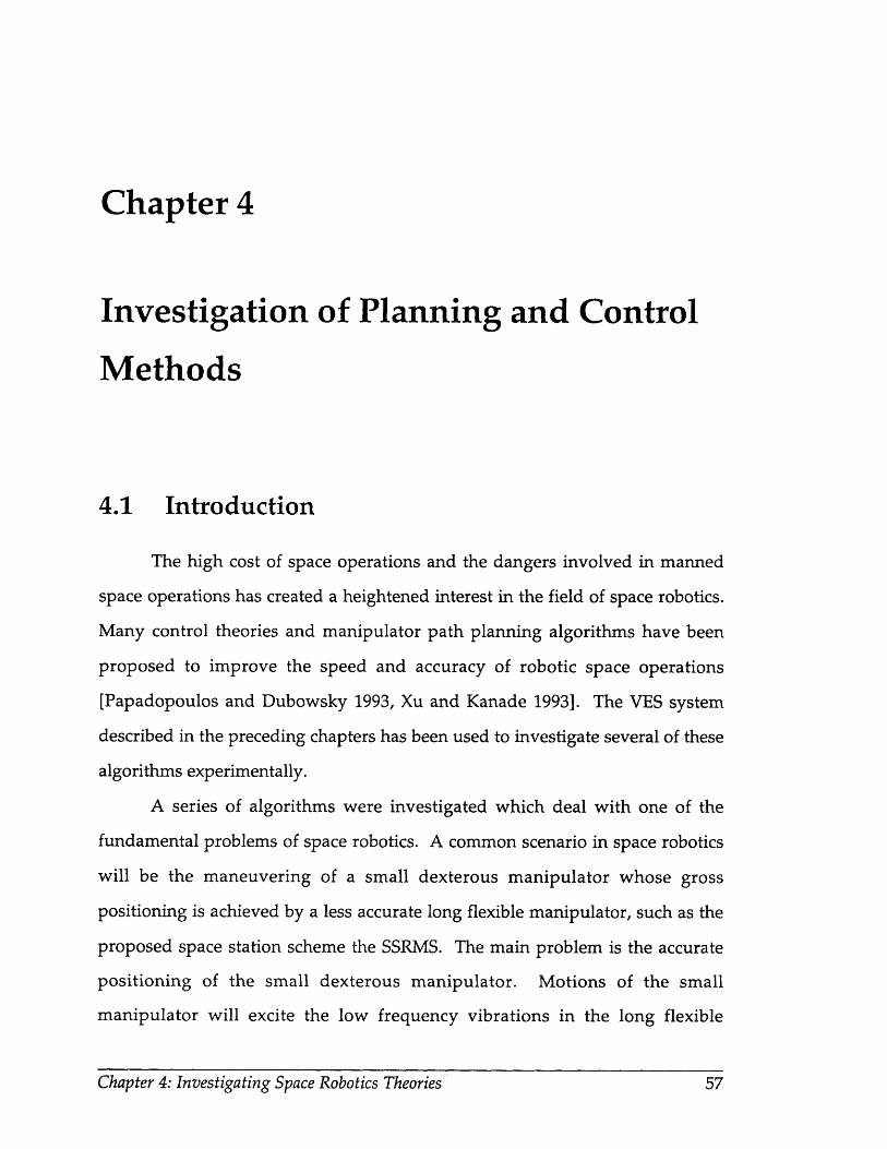
Figure 4-1 shows three cross sectional Coupling Maps for a PUMA 560 on

the two link beam structure described in Appendix A. These maps form three

faces of one quadrant of the manipulators joint space, the orientation of this

quadrant is also shown in Figure 4-1. For this system the symmetry of the joint

1 axis resulted in nearly vertical low coupling lines on the faces B and C for any

orientation of joints 2 and 3. This simplified the path finding task, since paths

could be generated for each surface of the cube almost independently. With

arbitrary initial and final end effector positions, I and F, two paths are

superimposed on this map. The "Bad Path" crosses over many dark lines, high

coupling areas, while the "Good Path" passes through the lighter lines, low

coupling areas, and travels parallel to the lines in high coupling areas. Following

minimum energy lines and avoiding high coupling regions is called the Hot Spot


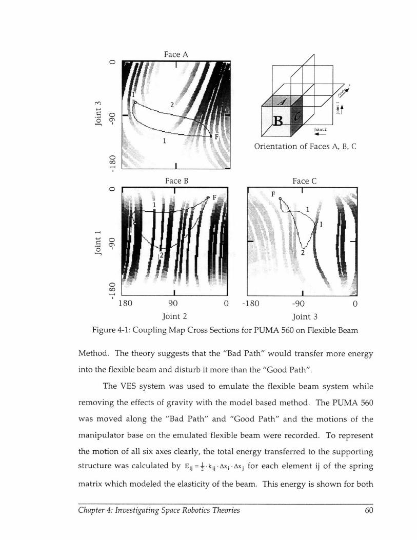
Face B0

o

00'--

WI

Orientation of Faces A, B, C

Face C

180 90 0

Joint 2

Figure 4-1: Coupling Map Cross Sections

-180

for PUMA

-90 0

Joint 3

560 on Flexible Beam

Method. The theory suggests that the "Bad Path" would transfer more energy

into the flexible beam and disturb it more than the "Good Path".

The VES system was used to emulate the flexible beam system while

removing the effects of gravity with the model based method. The PUMA 560

was moved along the "Bad Path" and "Good Path" and the motions of the

manipulator base on the emulated flexible beam were recorded. To represent

the motion of all six axes clearly, the total energy transferred to the supporting

structure was calculated by Eij = -kij -Ax i -Aj for each element ij of the spring

matrix which modeled the elasticity of the beam. This energy is shown for both


Face A

I

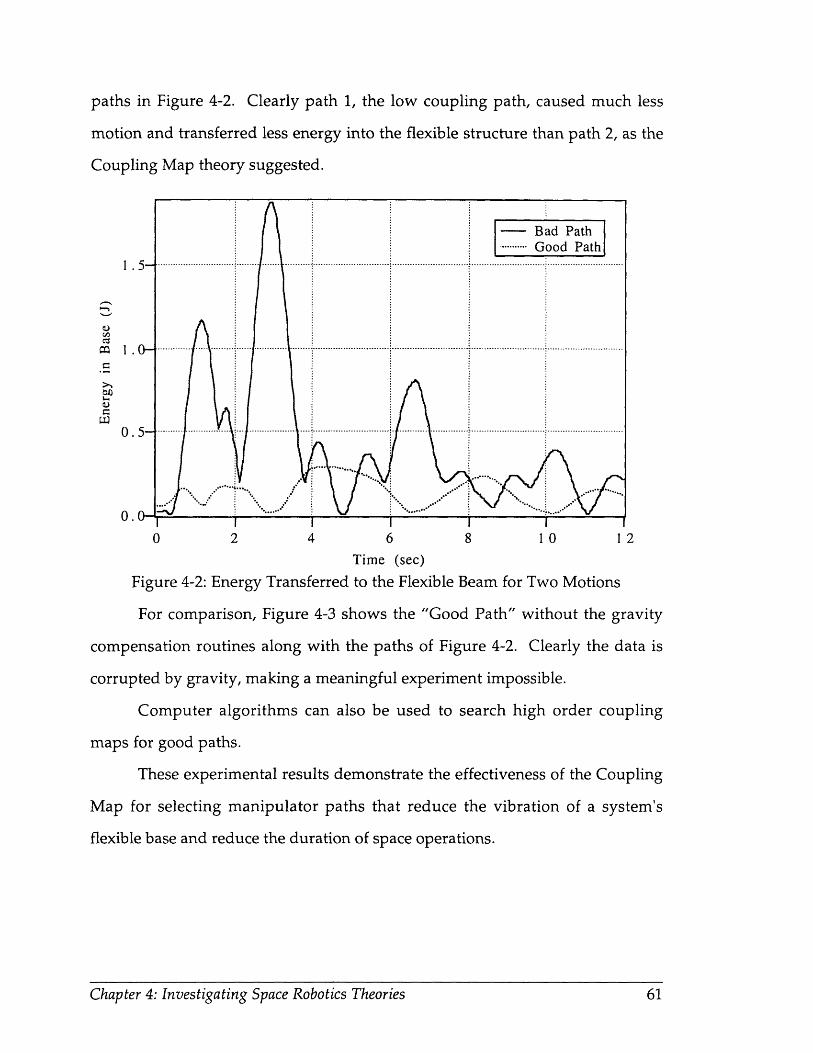
paths in Figure 4-2. Clearly path 1, the low coupling path, caused much less

motion and transferred less energy into the flexible structure than path 2, as the

Coupling Map theory suggested.

1 .5-

0 1.0-

0.5-

0.5-

nI I I I I I I0 2 4 6 8 10 12

Time (sec)

Figure 4-2: Energy Transferred to the Flexible Beam for Two Motions

For comparison, Figure 4-3 shows the "Good Path" without the gravity

compensation routines along with the paths of Figure 4-2. Clearly the data is

corrupted by gravity, making a meaningful experiment impossible.

Computer algorithms can also be used to search high order coupling

maps for good paths.

These experimental results demonstrate the effectiveness of the Coupling

Map for selecting manipulator paths that reduce the vibration of a system's

flexible base and reduce the duration of space operations.


Bad Path- Good Path

...........................---- ........................... .................................... .......................

S . ........................................... ..........................................................................................

.. . .... " .... .. .. ....... .. . "€, .... '..,.

....... .

2

CP

0 2 4 6 8 10 12

Time (sec)Figure 4-3: Energy Transferred to Beam With and Without Gravity

4.3 Pseudo-Passive Energy Dissipation

When vibrations exist in a long flexible beam system which is supporting

a dexterous manipulator, the manipulator itself can be used to damp out the

vibrations. An algorithm has been proposed which tunes the manipulators joint

controller gains to act as passive spring and damper elements to damp out the

vibrations [Torres 1993]. This method is called Pseudo-Passive Energy

Dissipation or PPED.

The basic PPED concept is very simple. The joint controller gains are

tuned to values which maximize the damping in the combined manipulator and

base system. The damping of energy works best if the manipulator is in a

configuration where the strain energy of the base is sensitive to small joint

motions. The Coupling Map Algorithm can be used to find these configurations.

For some systems, a concept known as the Virtual Manipulator can be used to

simplify the calculation of the best PPED gains [Torres 1993]. For many systems,


however, PPED requires calculating the full dynamic model of the manipulator

and its base structure.

4.3.1 The Virtual Manipulator Simplification

The virtual manipulator concept simplifies the analysis of space robotic

systems by allowing a manipulator to be modeled by a single mass with

massless links [Vafa 1987, Vafa and Dubowsky 1990]. This development is based

on applying the conservation of angular momentum principle to an arbitrary

free-floating manipulator.

A virtual manipulator can be constructed for any free floating robotic

system. The total mass of the manipulator is represented at the center of mass of

the system, and is called the virtual base. For a true free floating system, the

virtual base would remain stationary despite manipulator motions. Virtual links

connect the virtual base to the manipulators end effector. These links are always

parallel to the original links, and revolute joints always have the same angular

rotation as the actual joint (virtual prismatic joint motions are related to but not

the same as the originals). The lengths of the virtual links are calculated simply

as the ratio of mass in the present link and all previous links to the total mass in

the manipulator. Section B.5 shows the construction of a virtual manipulator for

a PUMA 560.

A virtual manipulator can also be constructed to go from the virtual base

to any point on the actual manipulator. For PPED analysis, it is convenient to

construct a virtual manipulator from the virtual base to the base of the actual

manipulator. Section B.5 also shows this construction for a PUMA 560.

Once the manipulator is modeled by its virtual manipulator the analysis to

find gains which maximize the system damping is quite simple. Figure 4-3

shows a manipulator and base system, and a simplified model which includes a


L2

virtual manipulator. Also shown in Figure 4-3 is an even more simplified model

of the system where the manipulator is replaced by a simple spring and damper.

A state space representation of the most simplified system can easily be

constructed. The values for the Ki's and Bi's can then be varied in an iterative

process which finds the gains Kd and Bd that produce the maximum damping in

the total system.

trL LUla ase4

t t l ,' ,-• • •'-NSLUL a

BaseMass

Virtual Manipulator Very Simple ModelModel on Flexible on Flexible

Manipulator on Flexible Base Base Model Base Model

Figure 4-3: Virtual Manipulator Modeling Concept

The Kd and Bd found can be easily converted to actual manipulator gains.

First the Cartesian space Kd and Bd must be converted to the virtual manipulator

joint proportional and derivative gains. Since the virtual manipulator has as its

end point the base of the supporting structure, the Kd and Bd are actually desired

end point compliance and damping values for the virtual manipulator. The

desired Kd and Bd values can be realized with the endpoint compliance control

method [Asada and Slotine 1986]. The standard analysis produces:

[Kvm] = [Jvm]T.[Kd][Jvm] (4.1)

[Bvm] = [Jvm]T[Bd][Jvm] (4.2)

where [Kvm] is a matrix of desired proportional gains for the virtual

manipulator joints,


Vit l B

[Bvm] is a matrix of desired derivative gains for the virtual manipulator

joints,

[Jvm] is the Jacobian matrix for the virtual manipulator.

Since the joints of the virtual manipulator are always parallel to the actual

joints and have the same basic geometry, the Jacobian matrix of the virtual

manipulator is the same as that of the robot with the virtual manipulator link

lengths substituted. For similar reasons, the control gains in the virtual

manipulator are the same as that of the actual robot. Therefore, the [Kvm] and

[Bvm] found in equation 4.1 and 4.2 are the actual manipulator PPED gains.

This approach has been used to successfully find gains for a simple two

degree of freedom planar space robot on a flexible base in simulation and

experimentation [Torres 1993]. Unfortunately, many flexible base systems have

significant stiffness in them, this makes them unsuitable for the free-floating

assumption that the virtual manipulator concept is based on. The scale of the

PUMA 560 robot used for our three dimensional VES experiments requires a

flexible base with a significant stiffness to be realistically practical. This suggests

that a different approach is required to demonstrate PPED on our system; a full

dynamic analysis.

4.3.2 Full Dynamic Analysis

When a space manipulators base structure has significant stiffness in it, the

virtual manipulator simplification cannot be used. A more complex full dynamic

analysis of the system is required. The concept behind PPED with full dynamic

analysis is quite simple, although the calculations are far more complex.

To find the appropriate PPED joint gains that will damp the most energy

out of the base, the full linearized dynamics of the combined manipulator and

base system must be written. For a complex system this can be quite difficult.


The full linearized dynamic equations for a PUMA 560 on an arbitrary linear

admittance model base are written in Appendix G.

The PUMA and base system dynamics are written in the form:

{d = }al. (4.3)

where X = [X, Y, Z, c, [3, y, q1, q2, q3] is the state vector containing the position

and orientation of the base and the joint displacements, and

[A] is a state space matrix.

To maximize the damping in the complex system, the damping of the 18

poles of matrix [A] must be maximized. An iterative searching algorithm was

written in matlab to search for joint gains which maximize this damping. At each

iteration, all 18 poles of the 9 DOF system were found. The damping of each

pole, weighted by the relative closeness to the origin, was used to estimate the

total system damping. The estimator used was:

Damping Estimator = i 1 - (4.4)

where n is the number of poles (18),

ýi is the damping ratio of pole "i", and

coi is the natural frequency of pole "i

This estimator was maximized interatively as the gains were changed.

The values which maximized the damping for a PUMA 560 with desired joint

angles of 450, 0o, 00 mounted on the beam system of Section A.5 were found to

be:

21 0 0[KpPED] 0 33 0 (4.5a)

0 0 20

72001[BPPED = 0 55 0 (4.5b)

0 0 17


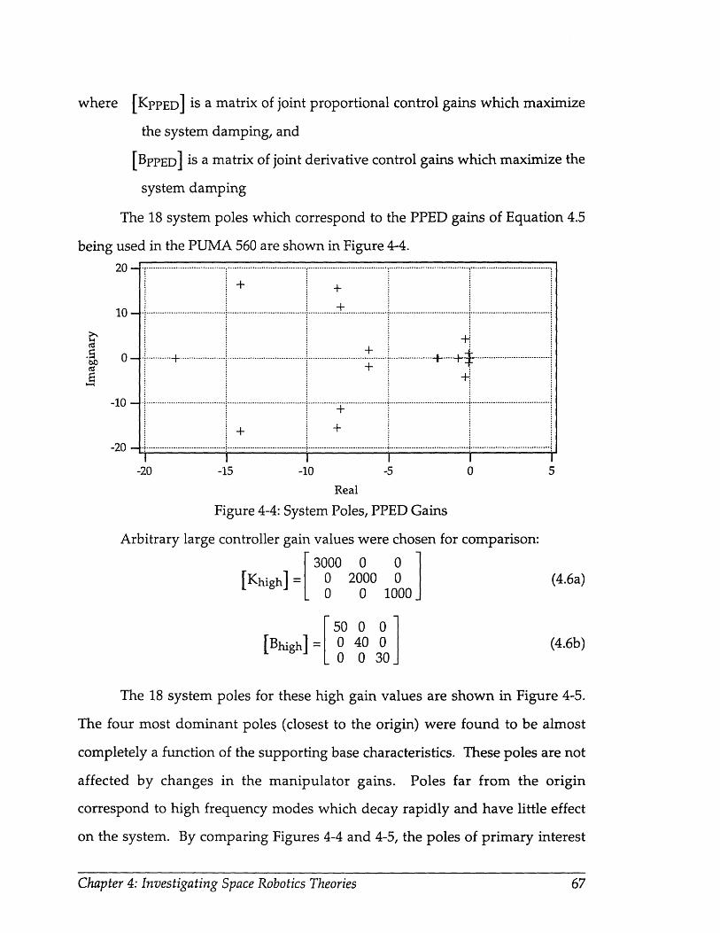
where [KPPED] is a matrix of joint proportional control gains which maximize

the system damping, and

[BPPED] is a matrix of joint derivative control gains which maximize the

system damping

The 18 system poles which correspond to the PPED gains of Equation 4.5

being used in the PUMA 560 are shown in Figure 4-4.20-

10-

1 00-

-10 -

-20 -

+ +

..

-----------· -+ ...... *+.... * -

I I I I I 1-20 -15 -10 -5 0 5

Real

Figure 4-4: System Poles, PPED Gains

Arbitrary large controller gain values were chosen for comparison:3000 0 0

[Khigh] 0 2000 0 (4.6a)0 0 1000

50 0 0[Bhigh] 0 40 0 (4.6b)

L 0 0 30

The 18 system poles for these high gain values are shown in Figure 4-5.

The four most dominant poles (closest to the origin) were found to be almost

completely a function of the supporting base characteristics. These poles are not

affected by changes in the manipulator gains. Poles far from the origin

correspond to high frequency modes which decay rapidly and have little effect

on the system. By comparing Figures 4-4 and 4-5, the poles of primary interest


(in the -2 through -5 range) can be seen to move closer to, or onto, the real axis,

increasing the damping of those poles and the whole system.

20-

10-

-0-

-10 -

-20 -

xx

xX

X* -1 ..........---- ------ --....................

X

-2 0 . .. ----------.................. .....I I I I I 1

-20 -15 -10 -5 0 5

Real

Figure 4-5: System Poles, High Gains

Both the PPED and high joint gains were used in simulations of the PUMA

560 on the flexible beam of Section A.5. In simulation, the base of the

manipulator was displaced to an initial position Y(0)= {.lm, .lm, .lm, 0", 0", 0'},

where Y(t) is defined in Equation 2.3, and then released. The total translational

motion of the base is shown versus time in Figure 4-6 for both the High gains,

and the PPED gains. The motion of the base in all six axes was used to calculate

the strain energy in the base. Figure 4-7 shows the total strain energy in the base

versus time, from a disturbed position with normal high gain values. Also

shown in Figure 4-7 is the strain energy for the same disturbance with the PPED

gains being used. Clearly the PPED gains allowed the manipulator to passively

damp out more of the vibrational energy in the system, reducing the total time it

took for the oscillations to die out. The same experiment could be performed

experimentally on the VES. Unfortunately, time does not allow the inclusion of

experimental results in this thesis.

Chapter 4: Investigating Space Robotics Theories 68

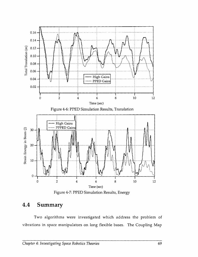
0.16 -

0.14 -

0.12 -

0.10 -

0.08 -

0.06 -

0.04 -

0.02 -

Time (sec)

Figure 4-6: PPED Simulation Results, Translation

2 4 6 8

Time (sec)

Figure 4-7: PPED Simulation Results, Energy

4.4 Summary

Two algorithms were investigated which address the problem of

vibrations in space manipulators on long flexible bases. The Coupling Map


. . . .. . . . . ... .

----- --- .... ..... ... .... .. .. .... .... .... .. .. .... ......... .... .... ....\. " :..\.......... .... ......, ...... ..... ........... ........

•-.--.- i·-- ·---- ·-- · ·...." -.. .. . .. . .. .. . . . . .... .. . . . . .. . . . . I... . . .. .. . . ....-" ;..

:- 'Y --- High Gains

S..........PPED

... f..... .\A...............\.. ..... ...

algorithm was shown to accurately plan paths which minimize the energy

transferred to the flexible base. The Pseudo-Passive Energy Dissipation concept

was shown to remove energy from an oscillating beam, allowing the settling

time to be reduced for a given disturbance. Both of these algorithms can be used

to reduce the time and cost of space robotic operations. Experimental

verification of the Coupling Map Algorithm was performed using the gravity

compensations routines on the VES.


Chapter 5

Improving System Performance with a

Digital Filter

5.1 Introduction

Excessive vibrations of the VES system were encountered during many

early attempts to perform experiments. Lowering the bandwidth of the legslave

controllers prevented vibrations, but caused further performance problems. An

analysis of this problem was conducted, and a digital filter was designed to

reduce the occurrence of vibrations and improve the response of the VES

system.

5.2 The Performance Problems

The first mode natural frequency of the assembled platform was

experimentally determined to be in the neighborhood of 10-13 Hz. This

frequency corresponds to transverse vibration of the individual legs, and

decreases with increasing length. The frequency of vibrations experienced

during operation was measured with an accelerometer attached to one leg,

Figure 5-1 shows the frequency range found by a spectrum analyzer. To avoid

Chapter 5: Improving System Performance with a Digital Filter

0 10 20 30

Frequency (Hz)

40 50

Figure 5-1: Platform leg natural frequencies

exciting these platform modes, low PD gains had been used, thus reducing the

platform bandwidth to about 2 Hz. Figure 5-2 shows the frequency domain

response of the original platform system without a digital filter. The low gains

response in Figure 5-2 shows the reduction in bandwidth necessary to avoid

vibrations. Running the platform with this reduced bandwidth created two

problems:

(1) Poor emulation of systems above 1Hz due to substantial positioning

errors.

(2) Excessive phase shift from the lowered gains caused increased

damping which was apparent in certain admittance model systems.

0 5 10 15 20

Frequency (Hz)

10 20 30

Frequency (Hz)


Figure 5-2: Original closed loop response with high and low gains

5.3 The Design Solution

To solve these problems, a digital filter was designed. The three basic

types of filter considered are shown in Figure 5-3. A Chebychev type 2 filter was

chosen to achieve a sharp corner attenuation with minimal phase shift from a

low order filter. The built-in first order attenuation (20dB per decade visible in

Figure 5-2) from the servo actuator was sufficient to prevent excitation of the

higher vibrational modes. The absence of higher order disturbance can be seen

0-

-10-

-0-20 -

a

" -30 -

-40 -

-50 - I I2 3 4

Frequency (Hz)

-50

a)

v,-1009

-150

Frequency (Hz)

Figure 5-3: Basic filter types, corner frequency of 10Hz

i· ·.... " .

i i iiI''I

3 4 5• °

I ~ °

3• ° 6


- Butterworth filter....

Chebychev type 1 f

(2dB ripple)Chebychev type 2 fstop band)

I

.. ,., ~lrrrvvvlCvvvvrv;-~;-;-;;:~C,

L- J. -·

requency (Hz

j

in Figure 5-1. The filter therefore needed to attenuate sharply in the desired

location, and minimally elsewhere. The design process was unique since the

filter is part of the platform closed loop control system. A model of the closed

loop actuator control system was constructed [Miiller 1992], and Matlab was

used to design filters within the closed loop system, to achieve a desired

response of the entire system. The block diagram of a continuous

approximation of the actuator system used for Matlab analysis is shown in

Figure 5-4.

digitalXd(•) E(s) units , volts amps K[ inches Xa(S)

N Y I r"1 j '~ rD/A I RS. r T [-

D/A Servo-Amp LengthGain Gain Servo Valve transducer

4TK 2 s1+ .

K1 clockticks

Feedback with Derivative control

Figure 5-4: Closed Loop Actuator Block Diagram

The general form of a digital recursive filter is:

Yn=bliXn + b2 *Xn-1 + b3*Xn-2 +... - a2*Yn-1 - a3*Yn-2 - ... (5.1)

where Yn is the output of the filter during digital step n, and

Xn is the input to the filter during digital step n.

Matlab can be used to generate several types of digital filter given the cycle time

of the digital system and the desired filter characteristics. Designing a digital

filter as an element within a complex closed loop system required several design

iterations.

The legslave board software was modified to add the digital recursive

filter calculations. This added a 2nd order filter component before the K1 gain in


Figure 5-4. Timing issues became critical because of the number of calculations

required for a 2nd order digital filter. The cycle time of the legslave boards was

increased from 1.023 msec. (831 Hz) to 1.705 msec. (587 Hz) to allow for the

added calculations. Since the Redslave board, which sends command positions to

the legslave boards, runs around 100Hz (10 msec. cycle time) it is still more than

five times slower than the legslaves. This insures that no commanded data will

ever be ignored.

The legslave board program, with the digital filter, was then burned into 6

EPROM's and the entire platform system was run. A sine wave was input to the

legslave boards (the Xd in Figure 5-4), and the magnitude and phase of the

legslave board output (the voltage out of the KD/A component of Figure 5-4)

was compared to the input wave. The platform was not allowed to run, so the

actual leg measurement in the feedback loop was constant. The change in

magnitude and phase shift were recorded to create a frequency response plot

which is compared to the Matlab designed filter in Figure 5-5. This procedure

confirmed the performance of the digital filter in the single closed loop system of

Figure 5-4.

The performance of the actual closed loop platform control system, which

is Figure 5-4 with the platform allowed to move, was tested by commanding the

platform to perform sine wave motion in the inertial Z-axis. Commanded and

actual position data for the platform were then converted to frequency and

magnitude data for a frequency response plot. This testing showed that the filter

did not completely attenuate the control signal in the lower end of the platform

natural frequencies. The filter was redesigned to achieve this goal, but at the cost

of an increasing phase lag. The increased phase lag would cause more damping

in the system, so several design iterations were made.


0 10 20 30 40Frequency (Hz)

Figure 5-5: Experimental verification of open loop filter design

5.4 Effect of Filter Location on Stability

After the digital filter was added to the legslave controllers, it was found

that some low mass admittance models were unstable. Even when the

manipulator was not moved, the platform would slowly oscillate with increasing

amplitude. The Matlab analysis of the closed loop actuator control loop [Figure

5-4] was modified to include the complete admittance model, closed loop


. ....... .... .

-10

d -15-

-20 -- AnalyticalS) ...... Experimental

-25-

-30-

-35-

0 5 10 15 20 25 30Frequency (Hz)

~--·------···-·---·-

actuator control, and force sensor feedback. This complete VES admittance

control loop is represented by the block diagram in Figure 5-6.

Payload Mass

Figure 5-6: VES Admittance Control Block Diagram

The digital filter was originally programmed to operate on the error

signal in the legslave controller as shown in Figure 5-7. Matlab analysis revealed

that although the actuator loop itself is stable, within the total VES control loop,

the digital filter caused instability. Admittance models with a mass less than half

of the actual mass on the force sensor (the payload mass in Figure 5-6) were

unstable, growing more unstable the lower the model's mass. A pole plot of the

VES system with the digital filter affecting the error signal and a low model mass

is shown in Figure 5-8. Two of the poles are clearly in the right half plane,

causing instability.

Figure 5-7: Digital Filter on Error Signal

Further analysis showed that if the filter were reprogrammed to operate

only on the feedback signal from the Temposonics cards, see Figure 59, the

entire VES closed loop system would be stable. Figure 5-10 shows the root locus

of the VES system with the digital filter affecting only the feedback signal.


V

f

6000

4000

L 2000

m00

E-2000

-4000

-6000-250 -200 -150 -100 -50 0 50

Real

Figure 5-8: VES Pole Plot, Filter on Error Signal

Simulations confirmed that the VES system, with the digital filter on the

feedback signal only, was stable for a wider range of admittance model values.

Very low stiffness systems are, however, still susceptible to small errors in the

force sensor.

I I

Figure 5-9: Digital Filter on Feedback Signal

At the time of the writing of this thesis, the digital filter had not been

moved to operate on the feedback signal. The results of the system and the

system response as shown in Sections 5.5 and 5.6 are based on Matlab analysis of

the leg control (Figure 5-7 or 5-9) only, and do not change significantly based on

the location of the filter. Only the stability of the total system for a small range

of admittance models (Figure 5-6) is affected.


............... ............. .........,... ......~ ........._ ..........

. . . . . . .. . . . . . . .. . . . . . . . ......... ..........---~ ------

.............. ...................

6000

4000

0 2000

E-2000

-4 0 0 0 .............. ................

-6000

C

-250 -200 -150 -100 -50 0Real

Figure 5-10: VES Pole Plot, Filter on Feedback Signal

5.5 Digital Filter Results

The specifications of the final filter design are summarized in Table 5-1. In

operation, the filter has performed well. The vibrations which had been caused

by disturbing the natural frequencies of the platform were removed for most

cases. An experiment was performed to compare the positioning errors in the

platform motion with the errors found before the digital filter was installed

[Kuklinski 1993]. The admittance model used for the experiment was a

decoupled model of varying parameters shown in Table 5-2, this model does not

represent any physically real system. With the PUMA 560 mounted on it, the

platform was displaced to an initial position Y(0)= {.2m, -.2m, .1m, 10", -10", 200",

where Y(t) is defined in Equation 2.3, and then released. The micro-gravity

motion which resulted was recorded, and the commanded and actual position

data were collected. Figure 5-11 shows that the positioning errors, the difference

between the commanded and actual position of a the platform, were reduced by

about 40% over the case of using low gains without the filter.


Table 5-1: Digital Filter SpecificationsType Chebychev Type 2

Order 2nd

Stop Band 4 dB

Corner Freq. 9 Hz

Sample Rate 587 Hz

Digital Recursive Coefficientsal = 1.0000 bl = 0.6040

a2 = 1.9002 b2 = 1.1969

a3 = 0.9113 b3 = 0.6040

As 4 + Bs 3 + Cs 2 + Ds + E

Fs4 + Gs3 + Hs 2 + Is + JLaplace Domain Coefficients

A= 0.00000000000854 F= 0.00000000001353

B= 0.00000000139394 G= 0.00000000616895

C= 0.00015641891531 H= 0.00024771331743

D= 0.00000019127013 I= 0.01347347243526

E= 0.99990021116393 J= 1.00000000000000

TABLE 5-2: Admittance Model for Positioning Error Experiment

Mass Matrix Spring Matrix Damping Matrix

Ml1 =500 kg K11=1500 N/m B11=500 N/m/s

M 22=500 kg K22=2500 N/m B22 =500 N/m/s

M 33=500 kg K33 =4000 N/m B33=500 N/m/s

M44 =250 kg-m2 K44 =1500 N-m B44=250 N-m/rad/s

M 55=250 kg.m 2 K55 =1000 N/m B55=250 N-m/rad/s

M 66=250 kg.m 2 K66 =2000 N/m B66=250 N-m/rad/s


0.0

0.0

S-0.0

0 2 4 6 8 10

Time (sec)

....... Alpha [X Axis]

.... Beta [Y Axis]Gamma [Z Axis]

1i~kYi:2

I I

,AV

0 2 4 6 8 10

Time (sec)

&- oo0 0.010-I -

= 0.000-o

' -0.010-

H

o 0.

o0.

0

. ,

04

02

00

....... X AxisY AxisZ Axis

0 2 4 6 8Time (sec)

....... Alpha [X Axis]

.... Beta [Y Axis]Gamma [Z Axis

10

0 2 4 6 8 10

Time (sec)

Without Filter With FilterFigure 5-11: Platform positioning errors

5.6 Choosing Platform Gains

In some orientations one or more of the legs are stretched longer than

they might during typical operation. This decreases their natural frequencies

such that they are not attenuated by the filter and may cause instability. This can

be alleviated by reducing the gains, again at the cost of a lower bandwidth and

more phase lag. Figure 5-12 shows the bode plots of the closed loop system with

the filter for a series of gains, based on simulations. It was found that K2 (see

Figure 5-4) had minimal effect on the bandwidth. It can therefore be set to a

maximum to reduce overshoot. For many applications, for low frequency

models when the platform stays near its home position, gains of K1=20,000

K2 =30000 will provide a good response. If vibrations are experienced, the

bandwidth can be lowered slightly by decreasing K1. Even if very low gains are


- 0.04-cO0 0.02-

CU0cr_

-,,,

L

,,

iI

~-/T~ i

1I

A_.

81

used to avoid vibrations on some experiments, the bandwidth and phase

characteristics are better than would be possible without the filter; compare

Figure 5-12 to Figure 5-2.

0

-20

-40

5 10 15 20 25

-10

-20

5 10 15 20 25

Frequency (Hz)

Figure 5-12: Bode Plot of Platform with Filter. {K2=30,000 K1=3,000-30,000}

The response to a unit step input of the closed loop leg control system,

including the filter, with varying gains is shown in Figure 5-13. This figure is

based on Matlab analysis.


Time (sec)

Figure 5-13: Platform Unit Step Response with Filter

5.7 Summary

A vibration problem encountered in the VES system was presented. An

analysis and the development of a digital filter to solve this problem was also

presented in detail. The effectiveness of the design was discussed. Finally, an

interesting application of control theory was detailed, the effects of positioning a

simple filter within a complex system.


5

Chapter 6

Conclusions

6.1 Contributions of This Work

This thesis describes the implementation of two micro-gravity emulation

routines on the VES II, the Learning Method and the Model Method. This

system can now be used to experimentally evaluate the dynamic interaction

between a robotic manipulator and its supporting structure in the micro-gravity

of space.

An overview of the basic components and operation of the VES II was

presented. An introduction was also given to the control architecture of the VES

II and the PUMA 560. The basic theory of the admittance control concept was

also presented.

The theoretical developments for gravity compensation were presented in

detail. The difficulties of estimating the effects of gravity were discussed. Two

methods were presented to compensate for gravity on the VES II, a learning

based method and a model based method. Experimental results were presented

which showed the accuracy of these methods.

Two algorithms were investigated which address the problem of

vibrations in space manipulators on highly flexible bases. The Coupling Map

algorithm was shown to accurately plan paths which minimize the energy

transferred to the flexible base. The Pseudo-Passive Energy Dissipation concept

was shown to remove energy from an oscillating beam, allowing the settling

time to be reduced for a given disturbance. Both of these algorithms can be used

to reduce the time and cost of space robotic operations.

A vibration problem encountered in the VES system was discussed. An

analysis and the development of a digital filter to solve this problem was

presented in detail. The effectiveness of the design was documented. Finally, an

interesting application of control theory was presented, the effects of positioning

a simple filter within a complex system.

Many details and calculations from this work are documented in the

appendices. This will hopefully provide a useful source of information for

researchers who will follow this work in the future.

6.2 Recommendations for Future Work

The primary contribution of this work was to bring the VES II system to a

state where it could reliably emulate micro-gravity. Some experimental work

was then performed with the system, but only a small sample of the possible

space robotic algorithms which could be tested. The most obvious and

important requirement for further work in this area is the application of the VES

II system to a number of control and planning algorithms for space robotics.

Although some improvement in the VES II will undoubtedly be made in

the future, there are no immediate problems to be solved. The primary addition

to the VES system should be the software which will expand the range of useful

experiments it can perform. Great care should be taken in the structure of new

software to fit it smoothly into the VES regime, but also to keep the total VES

software in a coherent state. The total software required to run a VES

experiment has already become very extensive, with no less than 6

programmers contributing. For the VES system to remain useful, all capabilities

and modifications of the software should be user friendly and well documented.

BibliographyAlexander, H. and Cannon, R., "An Extended Operational-Space Control

Algorithm for Satellite Manipulators," Journal of Astronautical Sciences, Vol. 38,

No. 4, 1990, pp. 473-486.

Arimoto, S., Kawamura, S., and Miyazaki, F., "Bettering Operation of Robots

by Learning," Journal of Robotic Systems, Vol. 1, 1984, pp. 123-140.

Armstrong, B., O. Khatib and J. Burdick, "The Explicit Dynamic Model and

Inertial Parameters of the PUMA 560 Arm." Proceedings of the IEEE International

Conference on Robotics and Automation, San Francisco, April 1986, pp. 510-518.

Corrigan, T. and Dubowsky, S., "Emulating Micro-Gravity in Laboratory

Studies of Space Robotics," 1994 ASME Mechanisms Conference, St. Paul, MN,

Sept. 1994.

Craig, J., Introduction to Robotics, Addison Wesley Publishing Co., 1989

Crane, C.D., Duffy, J. and Carnahan, T., "A Kinematic Analysis of the Space

Station Remote Manipulator System (SSRMS)," Journal of Robotic Systems, vol. 8,

no. 5, 1991, pp. 637-658.

Dubowsky, S., et al, "The Design and Implementation of a Laboratory Test

Bed for Space Robotics: The VES Mod II," 1994 ASME Mechanisms Conference, St.

Paul, MN, September 1994.

Dubowsky, S., Paul, I. and West, H., " An Analytical and Experimental

Program to Develop Control Algorithms for Mobile Manipulators," Proceedings

Bibliography

of the VIIth Symposium on Theory and Practice of Robots and Manipulators, Udine,

Italy, Sept., 1988.

Durfee, W., Idris, H. and Dubowsky, S., "Real Time Control of the MIT

Vehicle Emulator System," Proceedings of the 1991 American Control Conference,

Boston, MA, June 1991, pp. 2057-2058.

Erickson, J.D., Reuter, G. J. and Healey, K.J., " Technology for an Intelligent,

Free Flying Robot for Crew and Equipmet Retrieval in Space," Proceedings of the

Space Operations & Robotics Conference & Workshop, JSC, Houston, TX, July 1989.

Fresko, M., "The Design and Implementation of a Computer Controlled

Platform with Variable Admittance," S.M. Thesis, Department of Mechanical

Engineering, MIT, Cambridge, MA, January 1987.

Idris, H., Real-Time Control of a Six Degree-of-Freedom Vehicle Emulation

System, S.M. Thesis, Dept. of Mech. Engineering, MIT, Cambridge, MA, April

1992.

Iwata, T. et al., "Ground & Flying Testbed for the 2nd Generation Space

Robot," Proceedings of the i-SAIRAS '90, Kobe, Japan, 1990.

Juvinall, R. and Marshek, K, Fundamentals of Machine Component Design,

John Wiley and Sons, 1991.

Kuklinski, A., The Practical Implementation of an Experimental Tool for the

Dynamic Interactions in Mobile Manipulator Systems, S.M. Thesis, Department

of Mechanical Engineering, MIT, Cambridge, MA, June 1993.

Bibliography

Mayeda, H., K. Osuka and A. Kangawa, "A New Identification Method for

Serial Manipulator Arms," 9th IFAC World Congress, Vol II, 1984, pp. 2429-2434.

Mayeda, H., Yoshida, K. and Osuka, K., "Base Parameters of Manipulator

Dynamic Models," Proceedings of the IEEE International Conference on Robotics and

Automation, 1988, pp. 1367-1372.

Miller, U., Design of a Second Generation Experimental System for Studying

Mobile Manipulator Control, S.M. Thesis, Department of Mechanical

Engineering, MIT, Cambridge, MA, June 1992.

Olsen, Howard B. and Bekey, George A., "Identification of Parameters in

Models of Robots with Rotary Joints," Proceedings of the IEEE International

Conference on Robotics and Automation, 1985, pp. 1045-1049.

Papadopoulos, E. and Dubowsky, S., "The Kinematics, Dynamics and Control

of Free-Flying and Free-floating Space Robotics Systems," Special Issue on Space

Robotics, IEEE Transactions on Robotics and Automation, Vol. 9, No. 5, October

1993, pp. 1-13.

Sato, Y., et al., "Micro-G Emulation System Using Constant-Tension

Suspension for a Space Manipulator," Proceedings of the 1991 IEEE International

Conference on Robotics and Automation, Sacramento, CA, April 1991.

Shimoji, H., et al., "Simulation System for a Space Robot Using 6 Axes

Servos," Proceedings of the XIth IFAC Symposium of Automatic Control in Aerospace,

Tsukuba, Japan, 1989, pp. 115-120.

Bibliography

Spofford, J.R. and Akin, D.L. "Redundancy Control of a Free-Flying

Telerobot," AIAA Journal of Guidance, Control and Dynamics, vol. 13, No. 3, pp.

515-523, May 1990.

Stelman, N., "Design and Control of a Six-Degree-of-Freedom Platform with

Variable Admittance," S.M. Thesis, Department of Mechanical Engineering, MIT,

Cambridge, MA, May 1988.

Torres, M., "Modeling, Path-Planning and Control of Space Manipulators: The

Coupling Map Concept," Ph.D. Thesis, Department of Mechanical Engineering,

MIT, Cambridge, MA, February 1993.

Torres, M. and Dubowsky, S., "Path Planning for Elastically Constrained

Space Manipulator Systems," Proceedings of the IEEE International Conference on

Robotics and Automation, Atlanta, GA, May, 1993, pp. 812-817.

Ulrich, N. and Kumar, V., "Passive Mechanical Gravity Compensation for

Robot Manipulators," Proceedings of the IEEE International Conference on Robotics

and Automation, Sacramento, CA, April 1991, pp. 1536-1541.

Umatani, Y. and Yoshida, K., "Experimental Study of a Two Dimensional

Free-Flying Robot Satellite Model," Proceedings of the NASA Conf. on Space

Telerobotics, Pasadena, CA, January 1989.

Umetani, Y. and Holcomb, L., Co-Chairmen, Proceedings of the i-SAIRAS '90,

Kobe, Japan, November, 1990.

Bibliography

Vafa, Z., an Dubowsky, S., "The Kinematics and Dynamics of Space

Manipulators: The Virtual Manipulator Approach," The International Journal of

Robotics Research, August 1990.

Vafa, Z., The Kinematics, Dynamics and Control of Space Manipulators: The

Virtual Manipulator Concept. PhD Thesis, Department of Mechanical

Engineering, MIT, Cambridge, MA, November 1987.

West, H., Papadopoulos, E., Dubowsky, S. and Cheah, H., "A Method for

Estimating the Mass Properties of a Manipulator by Measuring the Reaction

Moments at its Base," Proceedings of the IEEE International Conference on Robotics

and Automation, Scottsdale, AZ, 1989.

Whittaker, W.L., et al., Space Robotics in Japan, NASA Japanese Technical

Evaluation Center Report (JTEC), January 1991.

Xu, Y. and Kanade T., Space Robotics: Dynamics and Control, Kluwer

Academic Publishers, 1993

Bibliography

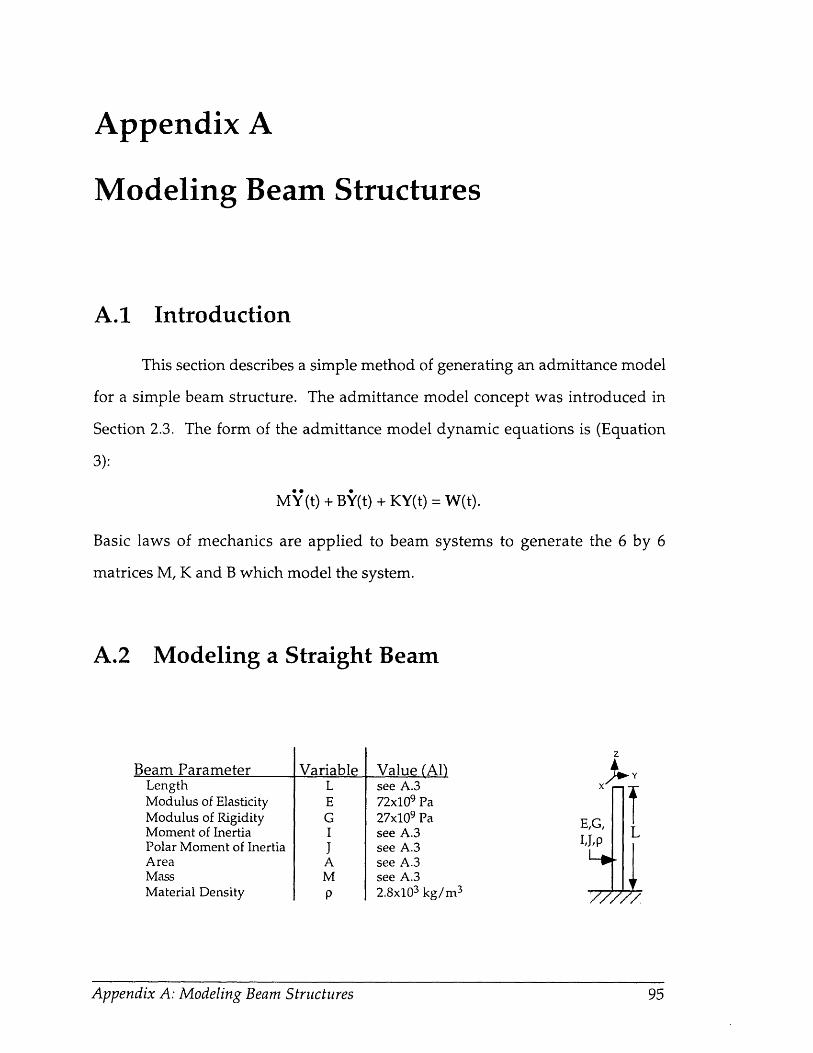
Appendix A

Modeling Beam Structures

A.1 Introduction

This section describes a simple method of generating an admittance model

for a simple beam structure. The admittance model concept was introduced in

Section 2.3. The form of the admittance model dynamic equations is (Equation

My(t) + BY(t) + KY(t) = W(t).

Basic laws of mechanics are applied to beam systems to generate the 6 by 6

matrices M, K and B which model the system.

A.2 Modeling a Straight Beam

Beam ParameterLengthModulus of ElasticityModulus of RigidityMoment of InertiaPolar Moment of InertiaAreaMassMaterial Density

Variable Value (Al)see A.372x109 Pa27x10 9 Pasee A.3see A.3see A.3see A.32.8x10 3 kg/m 3

Appendix A: Modeling Beam Structures

z

E,G, LIJ,p

'777-7

,

Analysis of a cantilever beam [Juvinall and Marshek 1991] produces the

familiar deflections and rotations as a function of Forces and Moments:-- 6X

80y

III

z

-87/I1ilz ..L v

sez -hz

X -FL 3 My-L 2

3E-1I 2.E.I

My*L Fx*L 2

80y-= EI 2.E.I

Fy.L 3 Mx*L2

-3EI - 2-E-I

Mx*Lx - E.I

E*A

6Z =MZ-LMz*LSz-G*J

Fy*L2

2*E.I

These equations can be used to produce a compliance matrix Q which is the

inverse of our stiffness matrix K {K=F/X, Q=X/F, K=Q-1}:

6XQ111- Fx

6YQ22 - Fy

6X LQ15 - My - EI

L3

- 3-E.I

L3

- 3-E-I6Y

Q24 - MX -L2

2*E*I8Z L

3 FZ EA

80xQ42 Fy= Fy

L22*E*I

60y L2

Q51 - Fx 2-E*I

S8z LQ66 Mz - G-J

80x LMx E-I

80y LQ55- My E-I


The total mass of the beam can be calculated easily:

mass = A-L-p

The equivalent mass seen at the end of the beam can be calculated by the kinetic-

energy method [Shigley 1967] as:

masseq = mass/2

The equivalent inertia seen at the end of the beam can be reasonably calculated

by the equivalent parameter method [Shigley 1967] as:

Ieq = masseqeL 2

The mass matrix can then be created as:

M 1 1 = M22 = M33 = masseq

M44 = M55= Ieq

M66 = Izz = 0

A damping matrix can then be chosen to create a 5% damping ratio for the

system:

B = 2..*K-M = .05

A.3 Straight Beam Experiments

The equations above produce the following

matrices for a 12 meter long hollow cylinder with a

diameter of 7 cm and a wall thickness of 6 mm made

of aluminum oriented vertically as shown in Figure

A-1:

Figure A-1: PUMA onVertical Beam


20 kg20

MassMatrix

0 0

0 20 kg 00 0 5 kg.m 2

0 0 0 00 0 0 0

0 00 00 00 0

2900 kg.m 2 0

0 2900 kg.m 2

StiffnessMatrix

312 N/m000

-1870 N-m/m- 0

0312 N/m

01870 Nm/mrn

00

00

7x10 6 N/mrn000

1870

15000

0 -1870 N/rad 0N/rad 0 00 0 0N.mrn/rad 0 00 15000 N-m/rad 00 0 2800 N.m/rad-

5 N/m/s0 5

Damping 0Matrix 0

0- 0

0 0N/m/s 0

0 1200 N/m/s0 0 660

0 0 00 0 00 0 0

N-m/rad/s 0 00 660 Nmrn/rad 00 0 2 N-m/rad-

Note that for a hollow circle:IC

I = -6 (Douter4 - Dinner4 ),

where Dinner = Douter - 2 - t,

and:

J=2 -I.

Appendix A: Modeling Beam Structures 98



Figure A-2: PUMA on VES Performing Simple Motion

Several experiments in this thesis use the same beam, a 12 meter long

hollow aluminum cylinder with a diameter of 7 cm and a wall thickness of 6mm,

oriented horizontally as shown in Figure A-2. A rotation matrix can be used to

produce the matrices for this horizontal beam:

000

2900 kg.m 2

00

0000

2900 kg.m2

0oo

7x10 6 N/m 00 312 N/m0 00 00 00 1870 N/rad

- 1870 N/rad

00

312 N/m0

1870 N/rad0

F--I - -,

I/UU N/m/r0Damping 0Matrix 0

0- 0

00

2800 N-m/rad00

0N/m/s

0 50

00

N/m/s0

0 00 0

0 00 1870 N/rad

-1870 N/rad 00 0

15000 N-m/rad 00 15000 N-m/rad-

000

2 N-m/rad/00

000

s 0660 N-m/rad

0 660

00000

N-m/rad-


MassMatrix

20 kg00000

020 kg

0000

00

20 kg000

StiffnessMatrix

00000

5 kgrn2-

r- ,

For several experiments in this thesis, the preceding horizontal beam

model was used in the VES, and the PUMA 560 was commanded to move its

shoulder joint through 180 degrees of motion, shown in Figure A-2. Details on

the PUMA 560 used are provided in Appendix B. The position and velocity

profiles of joint 1 are shown in Figure A-3. Joints 2 & 3 were held at 0".

270

225

180

135

0.0 0.5 1.0 1.5

Time (sec)

2.0

1.5

1.0

0.5

0.0 0.5 1.0 1.5

Time (sec)

Figure A-3: Position and Velocity Profiles of Simple Motion

2.0

2.0



A.4 Modeling a Complex Beamz

Beam Parameter

LengthModulus of ElasticityModulus of RigidityMoment of InertiaPolar Moment of InertiaAreaMassMaterial Density

VariableL1 and L2

EGIJAMP

Value (Al)see A.572x10 9 Pa27x10 9 Pasee A.5see A.5see A.5see A.52.8x10 3 kg/m 3

This more complex beam can be analyzed as the

superposition of two simple beams. To form a compliance matrix, it is easiest to

look at the translational and rotational effect of imposing individual forces and

moments on the end of this structure:

Fx-L 23

Fx -' X X 30E*IFx.L 2

2

y- 2-E-I

8X Fx-L1- E-A

5Z FxL2*L26Z 2*E*I

Fy.L 23

Fy = 8Y = 3E*I3-E-I

Y - Fy*L 13

3.E.

Fy-L 2*L1G*J

F x *L2.L 1 FX- L 22 L 1,V E*I X = L2*68Y= EI 1

Fy-L 22

8x=- 2.E.I

Fy*L22-L 1G.J

Fy*L126z-- 2-E.I

5Y = -L2*680 =

(Force on L2}

(Force on L1}

(Moment on L1)

(Force on L2}

(Force on L1}

(Moment on L1)

Z .L133-E-1

Fz*L128y - 2*E*I SX = L2 860y

Fz-Li2-L 22*E*I

{Force on L21

{Force on L1 I


Fz * 8Z E-L2A- E-A


Mx. L22M x = 5Y = - 2-E *I

Mx-L16x- GJ

My*L22

My * 5X _2*E*I

My-L128Z= 2E-I

66x- E*I

8Y = -L2 .*ex =

My*L26 0 Y EIl

My*L1- GJ

Mx.L 2 ,Li

GoJ

My*L2-L18X = L2 66Y =- G*JGoi

(Moment on L2}

{Moment on L1)

{Moment on L2}

{Moment on L1 }

Mz-L128Y - - 2 *E *I

(Moment on L2}

(Moment on L1}MzL18z EI

These terms can be used to produce a compliance matrix Q for this system:

8X L 23

Q- = Fx - 3-EI +

8Y L23

- Fy - 3-E-I

8Z L2 *L12

Q31 2~ Fx - 2*E*I

68x L 22

Q42- Fy - 2E°I

L 1 L 22.L 1EA -+ EL-E*A E*I

L3EI L22L1

L1 -L2G.J

6X L 22 L2 -L1

Q Mz - 2EI + E-I

z80 L12

Q62- Fy - 2-E-I

6X L2.L 12

- My - 2*E*I

6X L22 L2 -L1

SMz - 2E-I + E-I

6Y L22 L1*L2

Q24-Mx --2-E-I G.J8Y L1

2

Q26 - -26 MZ 2*E*I

3Z L2 L13

Fz - EA + 3E-1I

3Z L12

Q- -3 My - 2-E*I680 x L2 L 1

Q44- M - EI+ G+J

Q530y L12

Fz 2*EoI

56 y L2 L1- My - EI G*J80z L2 L1

Q66 Mz G-J E*I


Mz-L 2- G. J


The total mass of the beam can be calculated easily:

mass = A*(L1+L2)*P

The equivalent mass seen at the end of the beam can be calculated by the kinetic-

energy method [Shigley 1967] as:

masseq = mass/2

The equivalent inertia seen at the end of the beam can be reasonably calculated

by the equivalent parameter method [Shigley 1967] as:

IXXeq = masseqoL22

IZZeq = masseqeL12

IYYeq = masseq*(L12+L22 )

The mass matrix can then be created as:

M11 = M22 = M33 = masseq

M44 = IXXeq

M55= IYYeq

M66 = IZZeq

A damping matrix can then be chosen to create a 5 % damping ratio for the

system:

B = 2*4* M = .05

A.5 Complex Beam Experiments

Several experiments in this thesis use a complex bent beam model in the

VES with a PUMA 560 as shown in Figure A-3. The beam modeled is a long

hollow cylinder with L1 and L2 of 8 meters, a cross sectional radius of 9

centimeters and a wall thickness of 7 millimeters made of aluminum, the

equations above produce the following matrices:

Appendix A: Modeling Beam Structures 103Appendix A: Modeling Beam Structures 103


Figure A-3: PUMA Complex Beam

41 kg0

MassMatrix

StiffnessMatrix

976 N/m0

-770 N/m03698 N

-3698 N.m/m0

041 kg

00

0 041 kg 0

0 2600 kg-m2

0 00 0

49320 -770 N/mN/m 00 1592 N/m

3093 N-m/m 00 1233 N.m/mr

844 N-m/m

03093 N/rad

025548 N.m/rad

0

0 5302 N-m/rad

0 00 00 00 0

2600 kg-m2 00 5200 kg.m

2 -

-3698 N/rad 00 844 N/rad

1233 N/rad 00 5302 N-m/rad

23013 N-m/rad 00 7552 N.m/rad-

15 N/m/s0

Damping _ -10 N/m/sMatrix - 0

-4 N-m/m/s- 0

0 -10 N/m/s10 N/m/s

0 -12210 94 N/rad/s

0 34 N/m/s3 N-m/m/s 0 800 N.m/rad/s

0 1 N-m/m/s1 N-m/m/s

38 N

0 775 N0 98 N-m/rad/s

N/rad/s 00 41 N/rad/s

[/rad/s 00 195 N-m/rad/s

•m/rad/s 00 613 N-m/rad/s


Appendix B

The Anatomy of a PUMA 560

B.1 Coordinates and Definitions

dO

Figure B-1: PUMA 560 D-H Parameters

Denavit-Hartenburg Parameters of thedO = 0.22844 mdl = 0.672 md2 = -0.2435 m

PUMAd3 =a2 =a3 =

560 [Armstrong et. al. 1986]:0.098 m0.4318 m0.4331 m

Appendix B: PUMA Coordinates and Definitions 105

B.2 Link Masses and Inertias

Figure B-2: PUMA 560 link masses and position vectors [Armstrong et.al. 1986]

rOxro = 1rOy

Lroz

028S0.283O

r2x -0.364r2 = r2y = -0.006

,r2z [ 0.016

rixr= 1rly

Lrlz

r3xr3 = r3y

Lr3z

=

o0

.056,-0.142

= 00

Mo = 54.5 kg

M1 = 12.8 kg

M2 = 17.4 kg

M3 = 9.0 kg

6.6861o = 0-0

0.13012= 00

06.4650

00.5240

001.815

005.249

0.615I = 00

0I

0.01513= 0

0


00.6150

00.5740

000.081

001.424


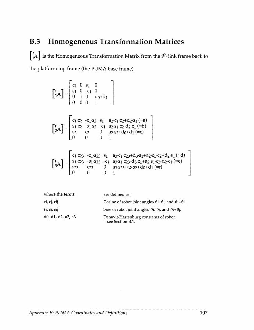
B.3 Homogeneous Transformation Matrices

[IA] is the Homogeneous Transformation Matrix from the ith link frame back to

the platform top frame (the PUMA base frame):

Cl 00 1o 0

sl-cl00

00do+d11

C1-C2 -C1"S2 Slt s2lC2 -Sl-S2 -C1

2 2 C2 0LO 0 0

c1"c23SC23

3A] S23-0

-C1'S23-SVlS23

C230

where the terms:

ci, cj, cij

si, sj, sij

dO, dl, d2, a2, a3

a2.cl.c2+d2-sl (=a)a2-slc 2-d2 -cl (=b)a2.s 2+do+dl (=c)1

a3-cl1C23+d3-sl+a2-1c-C2+d2-sl (=d)-Cl a3*slc23 -d 3.cl+a 2 'S1'C2-d2cl1 (=e)0 a3"s23+a2'S 2+do+d1 (=f)0 1

are defined as:

Cosine of robot joint angles ii, 0j, and 0i+0j.

Sine of robot joint angles *i, ij, and ii+tj.

Denavit-Hartenburg constants of robot,see Section B.1.


B.4 Jacobian Matrices

The Jacobian matrix to the center of mass of each link, ri in the link "i"

frame, is shown below.

J 11 -rlx.sl+rlz-cl1j 1 J12 = rlx.cl+rlz.sl

1J13 O

2Jl1 2J12 -r2x-sl-c2+r2y.sls2+r2z-cl-a2-slc2+d2-cl2j 2J 13 2J21 = r2x-cl-c2-r2y-c1-s2+r2z'sl+a2-C1-c2+d2sl1

2J22 2J23 .0-r2x-Cl*S2-r2y'C l-C2-a2-cl s2-r2x-sl"S2-r2y-Sl1C2-a2sls-s2r2x-c2-r2y-s2+a2-c2

J3JI 3J12 3J13 [-r3x*S1lC23+r3y'Sls23+r3z'Cl-a3"slC 23 +d3cl-a2sl*c2+d2"cl3j= 3 21 3J22 3J23 = r3x.Cl.C23-r3y*C1.S23+r3z.Sl+a3-c1-c23+d3.s1+a2-c1-c2+d2.s1

13J31 3J32 3J33 0-r3x-C1"S23-r3y-cl*c23-a3"cl"S23-a2"c1-S2-r3x'S1 S23-r3y'S1'C23-a3*s"lS23-a2"S1-S2r3x*c23-r3y's23+a3-c23+a2*c2

-r3x-cl s23-r3ycl- c23-a3-cl-s23-r3x-S1 s23-r3y-Sl*c23-a3sl s23r3x-C23-r3y.s23+a3*c23

Appendix B. PUMA Coordinates and Definitions 108Appendix B: PUMA Coordinates and Definitions 108

B.5 Virtual Manipulator to Endpoint

Figure B-3: PUMA 560 Virtual Manipulator to Endpoint

R1 = (0,0,0.629)

M1 = 54.5

L2 = (0,0,-0.056)

R2 = {0,0,-0.1875)

M2 = 12.8

L3 = {0.068,-0.006,0.016}

R3 = {0.364,0.006,0.082)

M3 = 17.4

L4 = 10.2911,0,0)

R4 = 10.142,0,0)

M4 = 9.0

Mtot = 93.4 kg

rl = R1 * M1/Mtot = 10,0,0.366)

12 = L2 * M1/Mtot = {0,0,-0.032}

r2 = R2 * (M1+M2)/Mtot = {0,0,-0.135}

13 = L3 * (M1+M2)/Mtot = (0.0488,-0.0043,0.0115}

r3 = R3 * (M1+M2+M3)/Mtot = (.329,0.0043,0.074)

14 = L4 * (M1+M2+M3)/Mtot = (0.263,0,0)

r4 = R4 * (M1+M2+M3+M4)/Mtot = (.142,0,0)

V1 = rl = (0,0,0.215)

V2 = r2 + 12= (0,0,-0.175)

V3 = r3 + 13= (0.377,0,0.0855)

V4 = r4 + 14= 10.405,0,0)

* The Virtual Manipulator concept is presented by [Vafa 1987, Vafa and Dubowsky 1990]


B.6 Virtual Manipulator to Base

Figure B-4: PUMA 560 Virtual Manipulator to Base

V1 = rl - R1 = {0,0 ,-0.263 }

V2 = r2 + 12 - R2 - L2 = (0,0,0.0765}

V3 = r3 + 13 - R3 - L3 = {-0.054,0,-0.0125}

V4 = r4 + 14 - R4 - L4 = {-0.0281,0,0}

D-H Parameters of Virtual Manipulator:

dl =-0.263

d2 = 0.0765

d3 = -0.0125

a2 = -0.054

a3 = -0.0281


Appendix C

Modeling a PUMA 560

C.1 Introduction

This section presents the equations and calculations required to form a

minimal model of a PUMA 560, in the form presented in Chapter 3. Recall that

the only manipulator model required to predict gravitational forces is the total

mass of the manipulator system. This procedure is exactly the same for any

manipulator system. The P vector which forms the manipulator model required

to predict gravitational moments, and the corresponding G matrix, change for

different manipulator geometries. Therefore, if a unique manipulator system is

to be used, the analysis presented in this section must be repeated.

C.2 Evaluating the P vector

A formula for the moment at the base of a general manipulator was

presented as Equation 3.6:Mx 1 0 0 0 rix b8gx

Mg= My = 0 1 0 0 •A . riy 'x (mi) .· gyMz, i=0 0010 1 0 riz, bgz

For the PUMA 560, the homogeneous transformation matrices presented in

Appendix B can be used to evaluate this equation:

Appendix C: Modeling a PUMA 560 111Appendix C: Modeling a PUMA 560 111

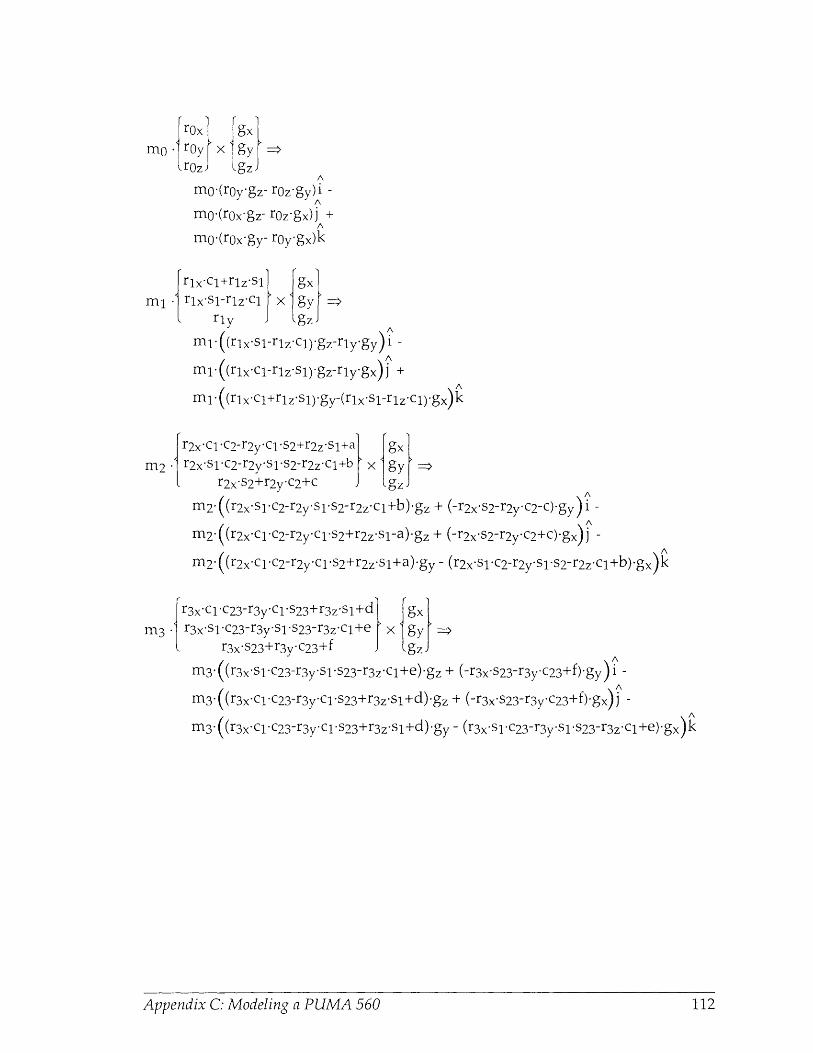
xOx xmo .•ry x{ gy

A

m0o(roy gz- roz-gy)i -A

mo*(rox'gz- roz*gx)j +

mo-(rox-gy- roy'gx)k

rlx'cl+rlz'sl gx

ml .rixl-s-rlz.cl x gyrly gz z

ml ((rlx-sl-rlz.Cl).gz-rly.gy)1 -A

ml'((rlx*cl-rlz-Sl)gz-rly'gx)j +

ml ((rlxcl+rlz'Sl)-gy-(rx-sl-rlz*Cl)-gx)Ak

r2x-clc 2-r2y-c l -S2+r2z.S1+a gxm2 r2x-sl C2-r2y'SlS2-r2zcl+b X gy

r2x'S2+r2y-C2+c gz,m2 ((r2x-sl-C2-r2y-slls2-r2z'cl+b).gz + (-r2x.s2-r2y-C2-c)-gy) 1 -

m2 ((r2x-cl-C2-r2y-cl.s2+r2z.sl-a).gz + (-r2x'S2-r2y.C2+c)-gx)j -

m2-((r2x.cl'c2-r2y-cl.s2+r2z.sl+a)-gy- (r2x.S1.c2-r2y.S1.s2-r2z'Cl+b).gx)k

r3xclC23-r3yC1S23+r3zSl+d fgxj

m3 .1 r3x-SlCc23-r3y-Sl-s23-r3z'cl+e x gyr3x.S23+r3y.C23+f g z

m3-((r3x'sl1c23-r3ySsl-S23-r3z-cl+e).gz + (-r3x-S23-r3y.c23+f)-gy)i -

m3-((r3x-cl1c23-r3y-cl-s23+r3z.sl+d)-gz + (-r3x-S23-r3y.c23+f)-gx) -

m3- ((r3x.cl-c23-r3ycl-s23+r3z-sl+d)-gy - (r3x-sl-C23-r3y'Sl'S23-r3z'C1+e)'gx)k

Appendix C: Modeling a PUMA 560 112

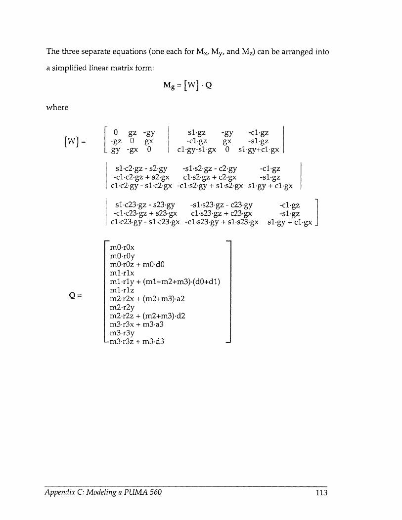
The three separate equations (one each for Mx, My, and Mz) can be arranged into

a simplified linear matrix form:

Mg= [W] Qwhere

sl gz-cl gz

cl-gy-sl.gx

-gy -cl.gzgx -sl.gz0 sl.gy+cl-gx

sl.c2.gz - s2-gy-cl.c2-gz + s2.gx

clc2-gy - sl.c2.gx -

s1-c23.gz - s23-gy-c1.c23-gz + s23.gx

cl.c23-gy - s1.c23.gx

-sl.s2.gz - c2-gycl.s2-gz + c2.gxcl-s2.gy + s.1s2-gx s

-s1-s23.gz - c23-gyc1.s23-gz + c23.gx

-cl.s23-gy + sl.s23-gx

-cl.gz-sl.gz

1.gy + cligx

-cl.gz-sl.gz

sl-gy + cl-gx

m0-r0xmOr0ymO-r0z + m0-d0ml-rlxml.rly + (ml+m2+m3)-(d0+dl)mlrlzm2.r2x + (m2+m3).a2m2-r2ym2.r2z + (m2+m3).d2m3.r3x + m3-a3m3-r3y

-rn.?r3~7 -4- ?·l.


[w] =0

-gzgy

gz0

-gx

-gygx0

-m-'1 r-'1z + ml-(


When linearly independent columns are removed:

Mg = [G] P

sl-gz-cigz

cligy-sigx

-cl gz-sl.gz

sl-gy+cl.gx

sl-c2.gz - s2.gy-cl.c2.gz + s2-gxclIc2gy - sl.c2-gx

sl.c23.gz - s23-gy-cl1c23.gz + s23.gx

cl.c23.gy - s1.c23.gx

mO-rOxm0-r0ymO-rOz +ml-rlx

-sl.s2-gz - c2-gycl.s2.gz + c2-gx

-ci-s2.gy + sl.s2-gx

-s1.s23-gz - c23-gycl.s23.gz + c23-gx

-c1-s23.gy + s1.s23.gx

ml-rly + m0-dO + (ml+m2+m3)-(d0+dl)

mlrlz + m2-r2z + (m2+m3)-d2 + m3-r3z + m3-d3m2.r2x + (m2+m3)-a2m2-r2ym3.r3x + m3-a3

_m3-r3y

where the terms:

gx, gx, gz

ci, cj, cij

si, sj, sij

dO, dl, d2, a2, a3

are defined as:

Gravity vector in platform top frame,see Equation 3.4

Cosine of PUMA joint angles -i, Oj, and ii+i3j.

Sine of PUMA joint angles -i, Oj, and Oi+i3j.

Denavit-Hartenburg constants of robot,see Appendix B.

The "j" axis component of link "i" center ofmass in link "i" coordinate frame.

Mass of link "i".

Appendix C: Modeling a PUMA 560 ii4

[G] =0

-gzgy

gz0

-gx

-gygx0

Appendix C: Modeling a PLIMA 560 114

C.3 Experimental Versus Measured MassParameters

The experimentally determined values for the P vector are compared to

values found by disassembly and measurement [Armstrong et al. 1986].

Experimentally Determined Values Physically Measured Values

M total: 95.065 kg...................... ............. 93.678 kg

P [ 1: 0.1028 kg-m ......................................... 0 kg-m

2: 0.8352 kg-m ............................................ 0 kg-m

3: 45.7104 kg-m ....................................... 54.54 kg-m

4: 0.1593 kg-m ....................... ................... 0 kg-m

5: -5.8440 kg-m .................................... -5.308 kg-m

6: 4.6137 kg-m ........................................... 5.065 kg-m

7: 0.1298 kg-m ....................................... ..- 0.1044 kg-m

8: 2.2527 kg-m ........................................... 2.617 kg-m

9: ] -0.0738 kg-m ............................. .. ....... ... 0 kg-m

Appendix C: Modeling a PUMA 560 115Appendix C: Modeling a PUMA 560 115

Appendix D

Coordinate Frame Transformation

.. geometric center/ .

sour Lop

ensor center

rm top framer

Figure D-1: Coordinate frame relationships

The coordinate center of measurements provided by the force sensor is

not located at the geometric center of the force sensor top, as show in Figure D-

1. Since the sensor frame and the top plate frame are orthogonal, the force

readings have the same magnitude in both frames. Converting from the sensor

frame to the platform top frame requires adding the moment components

resulting from the offset of the two frames:

Fx t = FY

Fyt = - FysFzt = -Fz s

MX t = Mx s -Fzsty +Fys't z (D.1)

My t = -My s+Fzstx0 +Fxstz 0

Mz t = -Mz s-FYstxo +Fxsty 0

where txo = -0.001 m, tyo = -0.00066 m, tzo = 0.18944

Appendix D: Coordinate Frame Transformation 116

Appendix E

The VES Micro-Gravity Handbook

E.1 Introduction

This Appendix describes in detail the procedures and precautions for

running the VES II system with the PUMA 560 to perform micro-gravity

emulation experiments. A summary of the steps required for a typical

experiment is followed by a details of each step. Charts are provided in Section

5.5 to determine platform gains for a desired bandwidth.

E.2 VES II Basic Rules

The VES II is a powerful machine and its operation for micro-gravity

emulation requires the coordination of two computers. There are many small

mistakes which can cause the computers to lock up, loosing communication and

control of the platform. Caution should always be exercised while operating the

VES and it should be watched constantly as long as the safety valves are open

and its position is being controlled by the hardware. The most important thing

to remember while operating the VES is:

Rule #1: If in doubt, press the panic button to freeze the platform.

Panic buttons are located on the main control crate and in the room with the VES

II. After freezing the platform, follow the VES II Freeze Recovery Procedure below

Appendix E: The VES Micro-Gravity Handbook 117Appendix E: The VES Micro-Gravity Handbook 117

The PUMA 560 is usually controlled by the PMAC with the built in VAL

controller standing by in free mode. If the power to the PMAC is shut off while

the VAL controller is in free mode, the PUMA 560 will collapse causing damage

to itself and possibly the VES II.

Rule #2: Do not shut off the crate power (even briefly) without

pressing the PUMA 560 panic button.

The PUMA 560 panic button is located on the modified teach pendant/control

module.

E.3 Basic Operating Procedures

VES II Start Up Procedures

Note: This procedure assumes that the platform is starting in the sleep position (all

legs retracted).

1) Calibrate the PUMA 560 position with VAL.

Turn the Unimation box power on with the switch on the control box.

The VAL monitor (connected to the Unimation box) will display an

initialization message.

Type "Y" and "return" twice to initialize VAL. The teach pendant will

display "No High Power".

Release the panic button and press the black power button to provide

power to the PUMA. (The PUMA can now be operated in joint mode,

etc.)

Press "comp" on the teach pendant to put the PUMA into computer

mode.

On the VAL monitor keyboard type "CA" for calibrate. The PUMA

will move each joint a short distance.

Type "speed 15" to limit the motion speed. Then type "do ready" to

move the PUMA to its home position.

Appendix E: The VES Micro-Gravity Handbook 118118Appendix E: The VES Micro-Gravity Handbook

Boot uP the Redslave. Blueslave and PMAC

Switch the power to the Huerikon crate to "on". The Redslave,

Blueslave and PMAC will boot automatically. Terminals can be connected

to the Redslave or Blueslave through the back of the crate to monitor the

boot up procedure.

The Redslave and Blueslave boot up process takes a minute or two.

3) Run "loadmkb" program on the Sun

In a Sun command window, move to the /home/platform/bin

directory.

Type "loadmkb", to run the program which allows you to transfer

admittance models from the Sun to the Redslave.

NOTE: This program must be started before the "testPlatform"

program is run or it will lock up the computers. Once "loadmkb" is

started it can be used to transfer new admittance models while

"testPlatform" is running, but when it is first started it sends default

information to the Redslave which will not work if the platform is already

running.

4) Set up the Redslave and Blueslave

In a Sun command window, type "rlogin blueslave" to remotely log

into the Blueslave. (the alias "blue" can be used)

In another Sun command window, type "rlogin redslave" to remotely

log into the Redslave. (the alias "red" can be used)

In the Redslave window, type "sendShMemArray" to define the array

of shared memory variables and set up memory sharing between the

Redslave and Blueslave.

5) Run "PumaMove" and move the PUMA to a safe position

In the Blueslave window type "ld < PumaStuff" to load the PUMA

control software.

Type "PumaMove" to run the PUMA control software.

On the PUMA control box, release the panic button and press the arm

power button. Press the "free" button, and switch levers "1", "2" and "3"

to the "+" symbol to release the first three joints from VAL control.

2)

Appendix E: The VES Micro-Gravity Handbook 119

Doing this will normally cause the joints to fall down, but when the

"PumaMove" software is initialized, it configures the PMAC to control the

first three joints.

At the main menu, choose "1 Robot Control".

Move joint #2 to 0 or 180 degrees.

NOTE: The PUMA must be in its home position when the PMAC is

started or the joint encoders will not be properly zeroed. The PUMA

must then be moved away from its home position before the platform is

moved or it will crash through the ceiling when the platform moves to its

home position.

6) Run "testPlatform" and start the platform

Make sure the red panic button on the platform control cart is pushed.

Start the hydraulic pump by pulling forward on the lever arm and

then quickly slamming it back as far as it will go.

In the Redslave window type "testPlatform" to run the platform

control software.

At the K1 and K2 gain prompts type any numbers and hit return. THE

PANIC BUTTON MUST BE PRESSED. This step makes the platform try to

start while the panic button is pressed. This functions as a quick check of

the platform safety routines. Error messages should appear saying that

the pressure is too low and the panic button is pressed. If no error

messages appear make sure the shared memory array has been sent or

start over.

Type cntrl-C to break out of the error messages.

Type "testPlatform" again.

Choose K1 and K2 gains based on bandwidth requirements and the

charts in Section 5.5. BEFORE HITTING RETURN AFTER GAIN K2: keep

your hand near the platform panic button, if anything will go wrong, this

is a likely time. Hit return for gain K2, and watch the platform and

control cart carefully for several seconds. (1) The platform should not

move AT ALL. (2) The lights on the legslave boards should remain on.

(3) The lights on the top row of current amplifier boards should go on. (4)

the main platform control menu should appear on the Redslave window.

If any of that does not happen, hit the panic button and start step six over.

Appendix F: The VES Micro-Gravity Handbook 120Appendix E: The VES Micro-Gravity Handbook 120

NOTE: A loud popping noise will be heard and the platform may shake

slightly as the safety valves and solenoids open. This is normal.

The platform is now under closed loop control in Idle mode.

7) Set the platActive flag

In the Blueslave window, choose "1 toggle platActive flag" to toggle

the platActive flag to "1". This flag tells the PumaMove software that the

platform is active and is passing force sensor information via sharedmemory.

NOTE: While the platform is running, it must constantly read the Data

Translation board to monitor the hydraulic fluid manifold pressure. If a

routine which reads the force sensor is run while the platform is running,both the Redslave and Blueslave will be trying to read the Data

Translation board at the same time. This will lock up both computers.

8) Load a calibration matrix and mass parameter vector

In the Blueslave window, choose "2 Load calibration matrix and P

vector". At the prompts choose the name of the most recent calibrationmatrix and mass parameter vector. (e.g. "massl5.dat" and "call5.dat")

9) Zero the force sensor

In the Blueslave window, choose "3 Zero the force sensor", then

choose "2 puma". This will set the zero of the force sensor based on the

gravity wrench estimate.

1 0) Verify the Gravity Compensation

In the Blueslave window, choose "4 Show measured and estimated

wrench". This option displays both the force sensor readings and the

gravity wrench estimation. These should be very close since the force

sensor was just zeroed based on the estimate.While in the Gravity Comp Test Menu, the PUMA can be moved to

new positions (option 1) and the new actual and estimated wrench can be

checked for estimation accuracy (option 3).


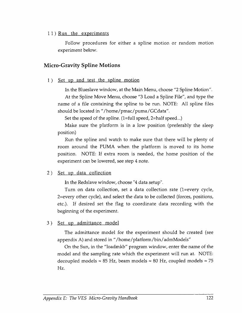
1 1) Run the experiments

Follow procedures for either a spline motion or random motion

experiment below.

Micro-Gravity Spline Motions

1 ) Set up and test the spline motion

In the Blueslave window, at the Main Menu, choose "2 Spline Motion".

At the Spline Move Menu, choose "3 Load a Spline File", and type the

name of a file containing the spline to be run. NOTE: All spline files

should be located in "/home/pmac/puma/GCdata".

Set the speed of the spline. (1=full speed, 2=half speed...)Make sure the platform is in a low position (preferably the sleep

position)Run the spline and watch to make sure that there will be plenty of

room around the PUMA when the platform is moved to its homeposition. NOTE: If extra room is needed, the home position of theexperiment can be lowered, see step 4 note.

2) Set up data collection

In the Redslave window, choose "4 data setup".Turn on data collection, set a data collection rate (1=every cycle,

2=every other cycle), and select the data to be collected (forces, positions,

etc.). If desired set the flag to coordinate data recording with the

beginning of the experiment.

3) Set up admittance model

The admittance model for the experiment should be created (see

appendix A) and stored in "/home/platform/bin/ admModels"

On the Sun, in the "loadmkb" program window, enter the name of the

model and the sampling rate which the experiment will run at. NOTE:

decoupled models = 85 Hz, beam models = 80 Hz, coupled models = 75

Hz.

Appendix F: The VES Micro-Gravity Handbook 122Appendix E: The VES Micro-Gravity Handbook 122

4) Run gravity compensation

In the Redslave window, choose "6 Active Gravity Comp". NOTE: If

the platform has not been moved yet, it will move to the home position

first.

Select the type of model being used - decoupled, coupled, or beam.

Set the sampling rate to the same value used in step 3.

Type "0" and return to run the admittance model in micro-gravity.

NOTE: The platform will not move until it receives a signal from theBlueslave.

NOTE: If extra room is required for the experiment, the platform

home position can be shifted down. Choose "3 MKB model", then choose

"6 Set Z offset", choose an offset (e.g. -.15m) to define a new home

position. Exit to the Main Menu. Choose "1 Ramp the Platform" and

move the platform to the new home position.

5) Run micro-gravity spline

In the Blueslave window, make sure that all the parameters were

properly set per step 1 above. Be sure to set delay time before and after

the experiment to see the base motion.

Select "9 Do It" to run the spline, the platform will start to move.

6) Reset the platform

If the experiment was successful, in the Redslave window choose "4

Data Setup", and then "11 Record Data" to record platform data from the

experiment.

In the Redslave window, choose "1 Ramp the Platform" and move the

platform to the home position for the next experiment.

Micro-Gravity Teleoperated Motions

1 ) Set up platform

Follow steps 2, 3 and 4 of VES II Spline Motion Experiments to set up

data collection, load an admittance model, and start gravity compensationon the platform.


2) Run gravity compensation and move the PUMA

In the Blueslave window choose "5 Run Gravity Compensation"

Enter the amount of time you would like to run gravity compensation.

If you would like to move the PUMA during the experiment, push the

"joint" button on the PUMA controller, and select "1 release PUMA to

VAL control" in the Blueslave window.

The platform will start moving. The PUMA can be moved with the

PUMA controller.

When the time has expired, type a key and return to re-establish

PMAC control of the PUMA, then put the PUMA in free mode (see step 5

of VES II Start Up Procedures.

3) Reset the platform

Follow step 6 of VES II Spline Motion Experiments .

VES II Shut Down Procedures

1 ) Move the platform to sleep position

In the Redslave window, choose "0 quit". The platform will then

prepare to move to the home position (all legs half extended). Make sure

the PUMA will not hit the ceiling during this motion. Type "0" and return

to allow the motion. The platform will then prepare to move to the sleep

position (all legs retracted). Type "0" and return to allow the motion.

2) Shut down the platform

Press the panic button.

Press the pump motor kill button, which is located next to the panic

button on the platform control crate.

3) Move the PUMA to its home position

In the Blueslave window, go to the Manual Mode Menu and move the

PUMA joints to 180',900,0'. The next time the VES II is started, the

calibration procedure will not be necessary.

Appendix E: The VES Micro-Gravity Handbook 124Appendix E: The VES Micro-Gravity Handbook 124

4) Shut down the PUMA

Press the panic button on the PUMA controller.

Shut off the power switch on the PUMA controller.

5) Shut down the Redslave, Blueslave and PMAC

Switch off the power on the Huerikon crate.

NOTE: If the platform will not be run again for some time, shut off the

power to the legslave boards, the temposonics cards, and the current

amplifiers. The switches are located at the back of the platform control

crate.

VES II Freeze Recovery Procedures

Note: This procedure assumes that the platform was frozen by pressing the panic

button.

1 ) If communications are locked, reboot

If communication with the Redslave and/or Blueslave were locked up:

press the panic button on the PUMA controller, then reboot the Huerikon

crate.

2) Restart the platform

In the Redslave window, type cntrl-C to break out of the platform

control software. If the computers were just rebooted, perform step 4) of

the VES II Start Up Procedures.

Start the platform by performing step 6) of the VES II Start Up

Procedures.

3) Move the platform to sleep position

Perform step 1) of the VES II Shut Down Procedures.

If the PUMA will hit the ceiling, start the PUMA and use the VAL

controller in joint mode to move the PUMA to a safe position.

4) Start over

Perform the VES II Start Up Procedures from the beginning. NOTE:

Be sure to reboot the PMAC if (1) the PUMA was moved under VAL


control, or (2) the PMAC was rebooted with the PUMA not in its home

position.

E.4 Laboratory Arrangement

In the summer of 1994, the VES was moved down the hall to a new

laboratory space. Figure E-1 shows the arrangement of the platform in the new

laboratory. This figure is a revision of Figure 4.4 in [Kuklinski 1993].

Appendix E: The VES Micro-Gravity Handbook 126126Appendix E: The VES Micro-Gravity Handbook

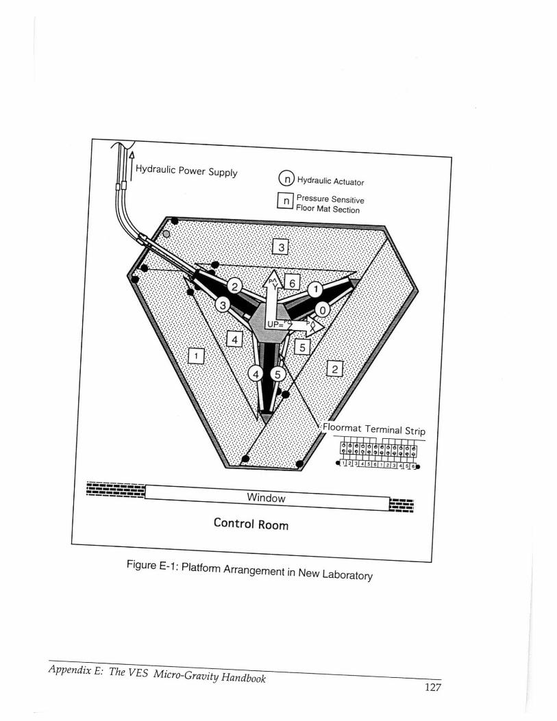
Figure E-1: Platform Arrangement in New Laboratory

Appendix E: The VES Micro-Gravity Handbook127

Appendix F

Force Sensor Noise

The force sensor used for these experiments is a very accurate instrument.

It does, however, have it limitations.

For these experiments, high frequency noise in the sensor can cause

significant error. Low bandwidth (20 Hz) Butterworth filters are used to reduce

this high frequency noise. Figures F-1 and F-2 show the force and moment

readings for all axes over a period of a few minutes. Clearly, a good deal of high

frequency noise remains in the system.

-- 195.0

-- 195.5N

-- 196.0

-- 196.5

Time (min)

Figure F-1: High Frequency Sensor Noise - Force

Appendix F: Force Sensor Noise

1.0-

0.8-

0.6-

-0.2-

............. ........... 1 1 ....... . .- .• . • • . •. • .• .i. ,. •Bl| : .. • a: i t :1' .. .. .... ........... ..

,IS..... . .............. ..... ....... ........ .........................i ", .. .. o' iF\ 1 __<......

.. ......... . ..." ... ... ...... .......... .... ..... .---- .... ........

I i I n •L i \I·' ' r...... ......... ................. .... ....~--· -· 1.....1.. ....... . . ....... .....i ......................... ........... ........ .li .................... 1 ... ......... • ....... i .... .. . •

............. .. ....... ........ . ...... .l ......... .......... .• ................. • .. ... ..,-- ............I jt I I'

rn-' II'........................ ......................... ........ ........... ..... ..... ................... .... ...... .... '... ..............· · · · ·- ·- · ·- · · · · · · · · · · ~·-···-····· ""' I'""'

128

0.2-

0.1--o-

-0.0-

-0.1-

-0.2-

0 3 4

Time (min)

Figure F-2: High Frequency Sensor Noise - Moment

Very low frequency drift in the force sensor can also degrade the quality

of this work. If the force sensor is zeroed often during an experiment, this is not

a significant problem. Figure F-3 and F-4 show the force and moment readings

of all the axes over a period of 8 hours. A serious drift in the sensor readings is

apparent.

4-

3-

2-

1-

0-

1-

2-

0I I I I I I I1 2 3 4 5 6 7

Time (hours)

Figure F-3: Low Frequency Sensor Noise - Force

-- 190

-- 191

-- 192

-- 193

-- 194

-- 195

- IK

Appendix F: Force Sensor Noise

..... ..... ..... ..... ..... ..... .... ..... ..... .... .... ..... ..... ..... ... --- .. ... .. ..... .... .... ....

~F /

..................... ........... ................ --- --......... ..................... --·---·--------- ........I I l~ j

/%r E-i .-- Iui

* *.; . -

--- --- --- - .... ... ... ... .. ... ... ... ... --- --- --- ----- ...... ............·~-r-

.. ... .... .. .... ... .. .. ... .... .. .. .. ... ... ..% .. .... .. .... .

··i·' ···- ··-- ·. .........···................................ ................... ........ .......... .........FY i

F

- I/vI

129

z 1

< 1.

-7 0.

> 0.

0.0.0.0

0 1 2 3 4 5 6 7 8

Time (hours)

Figure F-4: Low Frequency Sensor Noise - Moment

Avvendix F: Force Sensor Noise 130~IF T

Appendix G

Linearized Dynamic Model of PUMA

on a Flexible Base

Introduction

An analysis of the full dynamic model of a PUMA 560 on a flexible base in

zero gravity was conducted to allow calculation of joint controller gains for

PPED, see Section 4.3.2. The flexible base is represented by mass, spring, and

damper matrices called an admittance model, see Appendix A. Lagrange's

equation was used to construct the model. The nonlinear corriolis and

centrifugal forces were ignored to simplify the analysis.

The Model

18 state variables are required for this system:

ql, q2, q3 are the PUMA joint angles,

X, Y, Z, a , y,, are the translation and rotation of the PUMA base

Appendix G: Linearized Dynamic Model of PUMA on a Flexible Base 131

The kinetic co-energy and potential energy of the system can be written:

12+

T*= 1 ±2}T = Mb •2*~ *

M1 + 13

XiaM2. +tZy

X (M3. +t

,Zy

12

12. Ib

12 . I2

1 3-I3" [A]T

a&21 .10 "2 +2• 2I

~22

Y + q1 q2

2+

*K2citlA] T .1 1 +ql

* 2a 0S+ 0

S+ q9 3 q3

2X1 q2V [Kb] " + 2 .[Kr] q2

Sb q3

where bri is the link "i" position vector in the base frame, see Section B.3


X aM0- + J xbr0M .

2x br + [Jh1] .} +

2X br 2 + [J 2 ] 2 +

2[3]X br 3 +3 "q 3 +

The lagrangian formulation is written for each of the variables, and the corriolis

and centrifugal forces are ignored. The results can be put into the form:

[[M*]+ [I*]] . S + [iK*] S + [B*] .S =0

S = (X Y Z o f3y IT

MO+MI+M 2+M3M0 .ToT+M 1 -T1T+M 2.T2T+M3.T3TMI1 J1T+M2 'J2T+M3 'J3T

M0 -T0 +M1-T1 +M2 -T2+M3'T 3Mo.T0 .TOT+M 1 -Ti-T 1T+M2.T2.T2T+M3.T3.T3T

M1-J1T.TI +M2 "J2T.T2+M3 -J3T.T3

M 1.Ji+M2-J2+M 3'J3M1.T1T.J1+M2.T2T.J2+M3 .T3T-J3M1.J1T.J1 +M2.J2T.J2 +M3.J3T.J3

briz _briy0 brix-brix 0

and Ji is the Jacobian matrix of Section B.4

[122] = ['A] [II] ['A]T [2A] [12] ['A]T

[3A] [13] ['A]T

I22(3,1) I22(3,2)[132] = 12zS1+13z-S1 -I2z.C1-I3z'C1

L1 I3z'Sl -I3z'Cl

[123] = L1321

Ily+I2x-S22 +I2y.C2 2 +13x-(s2.C3+C2*S3) 2

[I33] = +13y'(C2-C3+S2'S3) 2

0L0

0 0

I2z+I3z 13zI3z 13z J

Appendix G: Linearized Dynamic Model of PUMA on a Flexible Base

where:

[M*] [

with:0

Ti = -brizbriy

[j*] =[

0]122 I23 ,withI32 133

122(3,3)00

133

r,_, l r,,_l

K = [Kb 0K , with Kb=base stiffness matrix and Kr=robot stiffness matrix

[B*] [ I, with Bb=base damping matrix and Br=robot damping matrix

iL...


Documents

Implementation and Application of Methods for Micro