Embed Size (px)
Citation preview

IMPERIAL COLLEGE LONDON
UNIVERSITY OF LONDON
ULTRASONIC WAVEGUIDE SENSORS FOR FLUID
CHARACTERISATION AND REMOTE SENSING
by
Frederic Bert Cegla
A thesis submitted to the University of London for the degree of
Doctor of Philosophy
Department of Mechanical Engineering
Imperial College London
London SW7 2BX
January 2006
Abstract
This thesis addresses two physical problems which both benefit from a new approach
using guided ultrasonic waves.
The first application relates to fluid characterisation. Conventional equipment for
fluid characterization has drawbacks due to the need of a straight, unobstructed
path across the fluid specimen, a perfectly parallel reflector, diffraction effects and
penetration problems in highly attenuating fluids. The use of ultrasonic waveguides
can alleviate these problems by separating the transducer from the measurement
area and by guiding the ultrasonic energy along a flexible waveguide of fixed ge-
ometry. The theoretical modelling, design and construction of a wave guide sensor
for fluid characterization of hot or radioactive fluids and liquids in general is pre-
sented. The sensor makes use of a guided interface wave. This wave was named the
quasi-Scholte wave because of its similarity to the Scholte wave that is widely known
in geophysics. It is a non-leaky guided wave that travels in a plate immersed in a
fluid. A substantial fraction of its energy travels in the fluid and is trapped at the
interface. It thus does not radiate energy away from the waveguide. This makes this
mode very sensitive to the fluid properties. It is shown that the fluid bulk velocity
and attenuation can be retrieved accurately using this method. Furthermore it is
shown that the use of other guided wave modes can be used to extract further fluid
properties so as to completely characterize the fluid acoustically.
The second application relates to non-destructive testing in harsh environments.
Conventional ultrasonic non-destructive testing uses a piezoelectric transducer close
to the area to be inspected. This becomes impossible above temperatures of about
300-400 C when conventional piezo-electric materials reach their Curie point and
become depolarized, which removes their ability to send or receive ultrasonic signals.
A remedy to this problem was found in using waveguides for remotely monitoring
thickness and defects within a structure under extreme conditions. The waveguide
separates the hot structure from the transducer which is located in a cool and
safe place. Essentially, this represents an acoustic cable along which ultrasound is
sent. The two main issues that had to be investigated are the wave propagation
along waveguides of different candidate geometries and the geometry and method of
2
attachment of the waveguide to the sample that is to be tested. The problems are
that the acoustic pulse has to remain strong and as undistorted as possible while
propagating along the waveguide, and when transmitting from the waveguide into
the sample. A system was designed and tested successfully at temperatures over
550 C.
3

Acknowledgements
The support from many people has considerably influenced the writing of this thesis.
I am most thankful to Prof. Peter Cawley and Dr. Mike Lowe for their excellent
guidance, stimulation and support as well as for giving me the opportunity to join
the NDT-Laboratory.
The help and discussions with several of my colleagues was also always helpful. In
a friendly environment I have learned plenty from every single member of the NDT-
group but most influential were Dr. Francesco Simonetti and Mr. Daniel Hesse. I
am also very grateful to Dr. Mark Evans and Dr. Thomas Vogt for their help and
advise with experimental equipment.
My gratitude to Prof. Richard Challis and Dr. Andrew Holmes from the University
of Nottingham should also be expressed. They carried out validation measurements
for results presented in this thesis. I am also very glad to have had the opportunity to
discuss some of the work presented here with Prof. Peter Nagy from the University
of Cinncinati who visited the Laboratory for a while.
Finally, I would also like to acknowledge the continued encouragement and support
from my family and my fiance Jaimini, without them the work would have been a
great deal harder.
4
Contents
1 Introduction 28
1.1 Motivation . . . . . . . . . . . . . . . . . . . . . . . . . . . . . . . . . 28
1.2 Thesis outline . . . . . . . . . . . . . . . . . . . . . . . . . . . . . . . 30
1.3 Figures . . . . . . . . . . . . . . . . . . . . . . . . . . . . . . . . . . . 33
2 Basic principles of bulk and guided waves 35
2.1 Wave propagation in bulk media . . . . . . . . . . . . . . . . . . . . . 35
2.2 Guided Waves . . . . . . . . . . . . . . . . . . . . . . . . . . . . . . . 39
2.2.1 Dispersion . . . . . . . . . . . . . . . . . . . . . . . . . . . . . 41
2.2.2 Mode shapes . . . . . . . . . . . . . . . . . . . . . . . . . . . 42
2.2.3 Wave propagation in rods and wires . . . . . . . . . . . . . . . 42
2.3 Existing techniques for material property measurements using wave-
guides . . . . . . . . . . . . . . . . . . . . . . . . . . . . . . . . . . . 43
2.4 Ultrasonic spectrometry . . . . . . . . . . . . . . . . . . . . . . . . . 45
2.4.1 Particle size determination . . . . . . . . . . . . . . . . . . . . 47
2.5 Summary . . . . . . . . . . . . . . . . . . . . . . . . . . . . . . . . . 48
2.6 Figures . . . . . . . . . . . . . . . . . . . . . . . . . . . . . . . . . . . 50
5

CONTENTS
3 Scholte mode and Quasi-Scholte mode Theory 57
3.1 The Scholte wave . . . . . . . . . . . . . . . . . . . . . . . . . . . . . 57
3.2 Theoretical modelling of the Scholte wave . . . . . . . . . . . . . . . 58
3.2.1 Influence of material properties on the Scholte wave . . . . . . 60
3.2.2 Modelling a viscous fluid . . . . . . . . . . . . . . . . . . . . . 61
3.3 Properties of the quasi-Scholte plate mode . . . . . . . . . . . . . . . 62
3.4 Quasi-Scholte mode sensitivity to fluid properties . . . . . . . . . . . 66
3.4.1 Sensitivity to the fluid bulk velocity . . . . . . . . . . . . . . . 66
3.4.2 Sensitivity to the fluid shear viscosity . . . . . . . . . . . . . . 67
3.4.3 Sensitivity to the fluid longitudinal bulk attenuation . . . . . 68
3.5 Liquid shear property determination using the SH0 mode . . . . . . . 68
3.6 Summary . . . . . . . . . . . . . . . . . . . . . . . . . . . . . . . . . 70
3.7 Figures . . . . . . . . . . . . . . . . . . . . . . . . . . . . . . . . . . . 72
4 Quasi-Scholte mode Experiments 88
4.1 Overview . . . . . . . . . . . . . . . . . . . . . . . . . . . . . . . . . . 88
4.2 Excitation of the Scholte and quasi-Scholte mode . . . . . . . . . . . 89
4.3 The setup . . . . . . . . . . . . . . . . . . . . . . . . . . . . . . . . . 90
4.4 SH wave attenuation measurements . . . . . . . . . . . . . . . . . . . 93
4.5 Ultrasonic Test cell . . . . . . . . . . . . . . . . . . . . . . . . . . . . 94
4.6 Results . . . . . . . . . . . . . . . . . . . . . . . . . . . . . . . . . . . 94
4.6.1 Newtonian Fluids . . . . . . . . . . . . . . . . . . . . . . . . . 94
4.6.2 Non-Newtonian Fluids . . . . . . . . . . . . . . . . . . . . . . 97
6
CONTENTS
4.7 Error considerations . . . . . . . . . . . . . . . . . . . . . . . . . . . 101
4.8 Summary . . . . . . . . . . . . . . . . . . . . . . . . . . . . . . . . . 104
4.9 Figures . . . . . . . . . . . . . . . . . . . . . . . . . . . . . . . . . . . 106
5 Non-dispersive wave propagation in thin flexible waveguides 116
5.1 Shear horizontal mode . . . . . . . . . . . . . . . . . . . . . . . . . . 116
5.2 Desirable waveguide characteristics . . . . . . . . . . . . . . . . . . . 118
5.3 Non-dispersive waveguides in the literature . . . . . . . . . . . . . . . 121
5.4 Wave propagation in rectangular strips . . . . . . . . . . . . . . . . . 122
5.4.1 Dispersion curves for rectangular strips . . . . . . . . . . . . . 124
5.5 Experimental work and preferential excitation of a single mode . . . . 128
5.5.1 Rods and Wires . . . . . . . . . . . . . . . . . . . . . . . . . . 129
5.5.2 Rectangular strips . . . . . . . . . . . . . . . . . . . . . . . . 131
5.6 Summary . . . . . . . . . . . . . . . . . . . . . . . . . . . . . . . . . 134
5.7 Figures . . . . . . . . . . . . . . . . . . . . . . . . . . . . . . . . . . . 135
6 Waveguide sources on half spaces 152
6.1 Strip sources on a half space . . . . . . . . . . . . . . . . . . . . . . . 153
6.1.1 Tangential anti-plane loading . . . . . . . . . . . . . . . . . . 154
6.1.2 Normal line source loading . . . . . . . . . . . . . . . . . . . . 157
6.1.3 Tangential line source loading . . . . . . . . . . . . . . . . . . 158
6.2 Circular sources on a half space . . . . . . . . . . . . . . . . . . . . . 159
6.3 Choice of the most suitable waveguide source on a half space . . . . . 160
7

CONTENTS
6.4 Wave reflection at the waveguide half space joint . . . . . . . . . . . . 163
6.5 Summary . . . . . . . . . . . . . . . . . . . . . . . . . . . . . . . . . 164
6.6 Figures . . . . . . . . . . . . . . . . . . . . . . . . . . . . . . . . . . . 166
7 Remote thickness gauging using a waveguide 178
7.1 The waveguide-structure joint . . . . . . . . . . . . . . . . . . . . . . 178
7.2 Experimental setups for thickness gauging . . . . . . . . . . . . . . . 179
7.2.1 Coupling with coupling agent . . . . . . . . . . . . . . . . . . 180
7.2.2 Welded and soldered strips . . . . . . . . . . . . . . . . . . . . 181
7.2.3 Clamped contact . . . . . . . . . . . . . . . . . . . . . . . . . 182
7.3 Room temperature thickness gauging with shear couplant . . . . . . . 183
7.4 High temperature measurements . . . . . . . . . . . . . . . . . . . . . 184
7.5 Summary . . . . . . . . . . . . . . . . . . . . . . . . . . . . . . . . . 186
7.6 Figures . . . . . . . . . . . . . . . . . . . . . . . . . . . . . . . . . . . 188
8 Conclusions 203
8.1 Thesis Review . . . . . . . . . . . . . . . . . . . . . . . . . . . . . . . 203
8.2 Findings . . . . . . . . . . . . . . . . . . . . . . . . . . . . . . . . . . 205
8.2.1 Fluid property measurements using the quasi-Scholte mode . . 205
8.2.2 Remote monitoring using a flexible waveguide . . . . . . . . . 207
8.3 Future work . . . . . . . . . . . . . . . . . . . . . . . . . . . . . . . . 209
A Global Matrix Solution 210
B Derivation of an approximate formula for the SH-wave attenuation213
8

CONTENTS
C Phase and group velocity 216
C.1 Retrieving phase and group velocity from measurements . . . . . . . 219
C.2 Retrieving phase velocity by cosine interpolation . . . . . . . . . . . . 221
C.3 Group velocity measurement using the zero phase slope . . . . . . . . 222
C.4 Velocity measurement using the amplitude spectrum method . . . . . 225
C.5 Preferred method for velocity evaluation . . . . . . . . . . . . . . . . 228
C.6 Figures . . . . . . . . . . . . . . . . . . . . . . . . . . . . . . . . . . . 230
References 247
9

List of Figures
1.1 Sketch of the of the principle of a) a ’dipstick’ interface wave measure-
ment of fluid properties and b) a fluid property measurement using a
conventional test cell setup. . . . . . . . . . . . . . . . . . . . . . . . 33
1.2 Sketch of the principle of the ’acoustic cable’ waveguide remote mon-
itoring system. . . . . . . . . . . . . . . . . . . . . . . . . . . . . . . 34
2.1 Phase velocity dispersion curves for a steel plate: Compressional
modes (—), Flexural modes (- - -) and Shear Horizontal modes ( · · ·) 50
2.2 5 cycle Hanning windowed excitation signal (a) and a prediction by
the DISPERSE [22] software of the signal after 0.5m propagation
distance as A0 mode on a 1mm thick steel plate (b) . . . . . . . . . . 51
2.3 Schematic of an infinite plate, its cross section and the polarisation
of the three fundamental plate wave modes. . . . . . . . . . . . . . . 52
2.4 Mode shapes of the (a) S0 mode, (b) A0 mode and (c) SH0 mode at
frequency thickness 0.1 MHz mm of a steel plate. (—) in-plane (z di-
rection) displacement, (- - -) out-of-plane (x direction) displacement,
(· · ·) in-plane (y direction) displacement . . . . . . . . . . . . . . . . 53
2.5 Mode shapes of the (a) S0 mode, (b) A0 mode and (c) SH0 mode at
frequency thickness 6 MHz mm of a steel plate. (—) in-plane (z di-
rection) displacement, (- - -) out-of-plane (x direction) displacement,
(· · ·) in-plane (y direction) displacement . . . . . . . . . . . . . . . . 54
10

LIST OF FIGURES
2.6 Phase velocity dispersion curves for a steel rod: Longitudinal modes
(—), Flexural modes (- - -) and Torsional modes (· · ·) [only order 0
and order 1 modes are shown]. . . . . . . . . . . . . . . . . . . . . . 55
2.7 Schematics of the different measurement methods in ultrasonic spec-
trometry: (a) through transmission (b) pulse echo (c) interferometer . 56
3.1 Sketch of the system used to study the Scholte wave . . . . . . . . . . 72
3.2 Mode shape of the Scholte wave on a Steel Water interface at 1 MHz
[(—) out of plane displacement, (- - -) in plane displacement, (· · ·)strain energy density ] . . . . . . . . . . . . . . . . . . . . . . . . . . 73
3.3 Contour map of the Scholte wave phase velocity to fluid bulk veloc-
ity ratio (Cscholte
Cfluid) as a function of density and longitudinal velocity
ratios (ρfluid
ρsolid,
Cl,fluid
Cl,solid) of the bulk materials (at fixed Poisson’s ratio
ν = 0.2865). The (+) sign indicates a steel/water interface. . . . . . . 74
3.4 Contour map showing the fraction of Scholte wave energy that travels
in the fluid (Efluid
Etotal) as a function of density and longitudinal velocity
ratios (ρfluid
ρsolid,
Cl,fluid
Cl,solid) of the bulk materials. (at fixed Poisson’s ratio
ν = 0.2865). The (+) sign indicates a steel/water interface. . . . . . . 75
3.5 The phase velocity dispersion of the quasi-Scholte mode on a steel
plate surrounded by water (see text for material properties). . . . . . 76
3.6 Mode shapes of the quasi-Scholte mode (water/steel) at frequency
thicknesses (a) 0.1 MHz-mm (b) 0.5 MHz-mm (c) 2 MHz-mm (in
plate only) for a 1 mm thick plate [(—) out of plane displacement, (-
- -) in plane displacement, (· · ·) strain energy density ] . . . . . . . . 77
3.7 Quasi-Scholte energy flow localised in the fluid (water) and plate
(steel) as a function of frequency [(—) Energy flow in fluid, (- - -)
Energy flow in plate]. . . . . . . . . . . . . . . . . . . . . . . . . . . 78
11
LIST OF FIGURES
3.8 Quasi-Scholte mode group velocities as a function of frequency for
different longitudinal bulk velocities (cl) (The other properties are as
in figure 3.10) . . . . . . . . . . . . . . . . . . . . . . . . . . . . . . . 79
3.9 Quasi-Scholte mode attenuation as a function of frequency for differ-
ent viscosities (η) at cl = 1800m/s (The other properties are as in
figure 3.10) . . . . . . . . . . . . . . . . . . . . . . . . . . . . . . . . 80
3.10 Total attenuation (—) of the quasi-Scholte mode and attenuation
due to shear leakage only (- - -) as a function of frequency for an
aluminium plate (ρ = 2700kg/m3, Cl = 6320m/s, Cs = 3130m/s)
immersed in glycerol (ρ = 1258kg/m3, Cl = 1900m/s, η = 1Pas) . . . 81
3.11 Attenuation dispersion curves of the quasi-Scholte mode for a 0.105
mm thick steel plate immersed in water of density 1000 kg/m3, bulk
velocity 1500 m/s and viscosity 1 mPas only (· · ·), viscosity 1 mPas
and longitudinal attenuation 0.001 Np/wl (- - -) and viscosity 1 mPas
and longitudinal attenuation 0.002 Np/wl (—). The attenuation unit
Np/wl stands for Nepers per wavelength. The quasi-Scholte mode
is attenuated by shear leakage due to viscosity and an additional
attenuation due to fluid longitudinal bulk attenuation. . . . . . . . . 82
3.12 The group velocity sensitivity of the quasi-Scholte mode to a change in
fluid bulk velocity for a 1mm steel plate surrounded by water (ρsteel =
7932kg/m3,Cl = 5959.5m/s, Cs = 3260m/s, ρwater = 1000kg/m3,
Cl = 1500m/s ). . . . . . . . . . . . . . . . . . . . . . . . . . . . . . . 83
3.13 The phase velocity sensitivity of the quasi-Scholte mode to a change in
fluid bulk velocity for a 1mm steel plate surrounded by water (ρsteel =
7932kg/m3, Cl = 5959.5m/s, Cs = 3260m/s, ρwater = 1000kg/m3,
Cl = 1500m/s ). . . . . . . . . . . . . . . . . . . . . . . . . . . . . . . 84
3.14 The attenuation sensitivity of the quasi-Scholte mode to a change
in fluid shear viscosity for a 1mm steel plate surrounded by water
with viscosity η = 1Pas (ρsteel = 7932kg/m3, Cl = 5959.5m/s, Cs =
3260m/s, ρwater = 1000kg/m3, Cl = 1500m/s ). . . . . . . . . . . . . 85
12

LIST OF FIGURES
3.15 The attenuation sensitivity of the quasi-Scholte mode to a change in
fluid longitudinal bulk attenuation for a 1mm steel plate surrounded
by water with viscosity ν = 1Pas and longitudinal bulk attenuation
of α = 0.01 np/wl (ρsteel = 7932kg/m3, Cl = 5959.5m/s, Cs =
3260m/s, ρwater = 1000kg/m3, Cl = 1500m/s ). . . . . . . . . . . . . 86
3.16 Schematic of the propagation of a Shear horizontal (SH) wave in a
plate. . . . . . . . . . . . . . . . . . . . . . . . . . . . . . . . . . . . . 87
4.1 Frequency versus wavenumber plot for the QS mode (—), the A0
mode (- - -) of a free plate and the leaky A0 mode (· · ·) of a steel
plate immersed in water (steel: ρ = 7932kg/m3, Cl = 6000m/s,
Cs = 3260m/s; water ρ = 1000kg/m3, Cl = 1500m/s) . . . . . . . . 106
4.2 Experimental setup . . . . . . . . . . . . . . . . . . . . . . . . . . . . 107
4.3 Schematic of the Transducer orientation and plate setup. . . . . . . . 107
4.4 Time trace at 500 kHz with aluminium plate 30 mm immersed in
Glycerol . . . . . . . . . . . . . . . . . . . . . . . . . . . . . . . . . . 108
4.5 Time trace at 3 MHz with stainless steel plate immersed a) 20 mm
and b) 80 mm in Water. . . . . . . . . . . . . . . . . . . . . . . . . . 108
4.6 Schematic of a conventional test cell. . . . . . . . . . . . . . . . . . . 109
4.7 Measured (+) and theoretically predicted (—) (a) group velocity and
(b) attenuation of the quasi-Scholte mode on a 0.94 mm thick alu-
minium plate immersed in glycerol (ρ = 1258kg/m3, Cl = 1930m/s,
η = 0.82Pas) . . . . . . . . . . . . . . . . . . . . . . . . . . . . . . . 110
4.8 Measured (+) and theoretically predicted (—) (a) group velocity and
(b) attenuation of the quasi-Scholte mode on a 0.94 mm thick alu-
minium plate immersed in honey (ρ = 1400kg/m3, Cl = 2140m/s,
η = 19.2Pas) . . . . . . . . . . . . . . . . . . . . . . . . . . . . . . . 111
13
LIST OF FIGURES
4.9 Literature data from Povey [1]for distilled water (—) and 5 % ethanol-
distilled water mixture (- - -) for the bulk velocity and data from the
inversion of the quasi-Scholte mode measurement (distilled water o,
5 % ethanol-distilled water �) . . . . . . . . . . . . . . . . . . . . . . 112
4.10 Quasi-Scholte mode group velocity obtained by forward modelling
using the fluid bulk velocity and attenuation from the ultrasonic test
cell measurement (- - -) and by direct measurement of the quasi-
Scholte mode (—) [Snowtex-ZL (o), Syton-HR50 (�), SILMIKRON-
50 (+), SILMIKRON-150 (�)]. The errorbars indicate errors due to
the 0.5 % uncertainty in evaluating the immersion depth. . . . . . . 112
4.11 Quasi-Scholte mode attenuation obtained by forward modelling using
the fluid bulk velocity and attenuation from the ultrasonic test cell
measurement (- - -) and by direct measurement of the quasi-Scholte
mode (—) [Snowtex-ZL (o), Syton-HR50 (�), SILMIKRON-50 (+),
SILMIKRON-150 (�)]. The error bars indicate the standard error of
the signal and a curve fit (see text). . . . . . . . . . . . . . . . . . . . 113
4.12 Fluid bulk velocity from the ultrasonic test cell measurement (- -
-) and by inversion of the quasi-Scholte mode measurement (—).
[Snowtex-ZL (o), Syton-HR50 (�), SILMIKRON-50 (+), SILMIKRON-
150 (�)] The errorbars indicate errors due to the 0.5 % uncertainty
in evaluating the immersion depth. . . . . . . . . . . . . . . . . . . . 114
4.13 Fluid bulk attenuation from the ultrasonic test cell measurement (-
- -) and by inversion of the quasi-Scholte mode measurement (—)
[Snowtex-ZL (o), Syton-HR50 (�), SILMIKRON−50 (+), SILMIKRON−150
(�)]. The error bars indicate the standard error of the signal and a
curve fit (see text). . . . . . . . . . . . . . . . . . . . . . . . . . . . . 114
4.14 Raw measurement data (—) and the quadratic curve fit (- - -) for a
Snowtex-ZL sample. . . . . . . . . . . . . . . . . . . . . . . . . . . . 115
14
LIST OF FIGURES
5.1 Temperature distribution along a (—) steel wire of 0.5mm radius, a
(- - -) steel rod of 10mm radius and a (· · ·) rectangular steel strip
of 15mm and 1mm width and thickness respectively. One end cross
section of each is maintained at 600◦C while the air surrounding the
waveguide is at 25◦C. Calculation after Mills [65] with steel conduc-
tivity of k = 15 W/m/K and heat transfer coefficient of free convec-
tive air hc = 1 W/m/K. . . . . . . . . . . . . . . . . . . . . . . . . . 135
5.2 Sketch of the ”hockey stick” system for fluid flow metering (after
Lynnworth [79]) . . . . . . . . . . . . . . . . . . . . . . . . . . . . . . 136
5.3 Sketch of the geometry of the FE model used to obtain the dispersion
curves of a strip of rectangular cross section (see text for dimensions). 136
5.4 Sketch of the frequency-wavenumber results obtained from a FE eigen
solver at different cyclic orders. . . . . . . . . . . . . . . . . . . . . . 137
5.5 Sketch of the frequency-wavenumber results transformed into the
phase velocity frequency domain. . . . . . . . . . . . . . . . . . . . . 137
5.6 Dispersion curves for a 1mm thick and 30mm wide rectangular steel
strip determined by FEM a) frequency-wavenumber b) phase velocity
frequency. Two interesting modes that correspond to the lowest order
shear horizontal mode (SH*) and the lowest order flexural mode (A0*)
that is symmetric with respect to its width are highlighted by the bold
dashed (- - -) lines. . . . . . . . . . . . . . . . . . . . . . . . . . . . . 138
5.7 Modulus of the displacement mode shape in the x, y and z direction
of the A0* mode at 2.5 MHz. . . . . . . . . . . . . . . . . . . . . . . 139
5.8 Modulus of the displacement mode shapes of the SH* mode in the x,
y and z directions at a) 0.14, b) 0.5 and c) 2 MHz of a 15mm wide
and 1mm thick rectangular steel strip. . . . . . . . . . . . . . . . . . 140
5.9 Evolution of the SH* mode y displacement mode shape of a 30mm
wide and 1mm thick steel strip over a range of frequencies. . . . . . . 141
15

LIST OF FIGURES
5.10 Sketch of the 2D plane stress model that was defined in ABAQUS to
analyse the effect of different excitation force profiles. . . . . . . . . 141
5.11 Y-direction displacement field output of the plane stress steady state
frequency domain finite element model of a steel strip (15mm) under
a) rectangular excitation force profile b) exact mode shape excitation
force profile c) triangular excitation force profile across the width of
the strip. The difference between cases b) and c) is highlighted in
figure 5.12. . . . . . . . . . . . . . . . . . . . . . . . . . . . . . . . . . 142
5.12 Zoom on the Y-direction displacement fields of figure 5.11 b) and
c) highlighting the subtle difference between the field excited by a
triangular forcing profile and the exact mode shape forcing profile. . 143
5.13 Phase velocity curves for the SH* mode of a 1mm thick rectangular
steel strip of width indicated in the legend and traced using the FE
eigensolver routine written by Wilcox et al. [81] and the DISPERSE
software [22] . Note that the cut-off of the modes occurs at the same
frequency-width product (i.e. the cut-off of the 30mm wide strip
occurs at half the frequency of the cut-off of the 15mm wide strip). . 144
5.14 Schematics and pulse echo signals received from a) a solid 5mm diam-
eter and 160mm long steel rod b) a bundle of 18 steel wires of diameter
1mm. The group velocity dispersion curve for rod/wire waveguides
is also shown in c). . . . . . . . . . . . . . . . . . . . . . . . . . . . . 145
5.15 Pulse echo signal (0.8 MHz) excited and received by a 1mm diameter
and 0.5mm thick piezo disc attached to a 0.5m long steel wire of 1mm
diameter. . . . . . . . . . . . . . . . . . . . . . . . . . . . . . . . . . 146
5.16 2 MHz centre frequency SH* signal received in pulse echo mode from
a standard shear transducer coupled to the end of a 15mm wide and
1mm thick stainless steel strip. . . . . . . . . . . . . . . . . . . . . . . 146
16
LIST OF FIGURES
5.17 a) Sketch of the in-plane laser doppler vibrometer scanning configura-
tion along the strip. b) Two dimensional fourier transform of in plane
surface displacements (polarised in the width direction of the strip)
along the centre line of 1mm thick and 30mm wide the steel strip.
The dashed line (- - -) shows the predicted dispersion relation for the
SH* mode of steel (ρ = 7932kg/m3, Cl = 6000 m/s, Cs = 3060 m/s). 147
5.18 10 cycle 2 MHz centre frequency A0* signal received in pulse echo
mode from a standard shear transducer coupled to the end of a 30mm
wide and 0.2mm thick stainless steel strip. . . . . . . . . . . . . . . . 148
5.19 a) Sketch of the out-of-plane laser doppler vibrometer measurements
on a strip. b) Two dimensional Fourier Transform of the out-of-plane
displacements of the centre line of a 0.2mm thick and 30mm wide
steel strip along the centre line of the strip. The dashed line (- -
-) shows the predicted dispersion relation for the A0* mode of steel
(ρ = 7932kg/m3, Cl = 6000 m/s, Cs = 2840 m/s). . . . . . . . . . . 149
5.20 2 MHz centre frequency signal received in pulse echo mode from a
standard shear transducer coupled to the end of a 30mm wide and
0.2mm thick stainless steel strip a)just touching a water bath and b)
immersed 70mm into a water bath. . . . . . . . . . . . . . . . . . . . 150
5.21 Group velocity for the quasi-Scholte mode of an infinite plate in water
as predicted by DISPERSE (thin line) and measured group velocity
of a thin stainless steel strip (0.2mm thick, 30mm wide and 300mm
long) immersed in water (bold line). . . . . . . . . . . . . . . . . . . . 151
6.1 Schematics of the different line source (2D) loading conditions that
were considered a) anti-plane shear loading b) normal loading c) tan-
gential shear loading. The sources are infinitely long in the z direction
and have a finite width in the x direction (from -a to a). . . . . . . . 166
6.2 Contour plot of the uz displacement field magnitude for a SH-line
source on a half space of steel. . . . . . . . . . . . . . . . . . . . . . . 167
17
LIST OF FIGURES
6.3 Angular distribution of the magnitude of the displacement for a) com-
pressional waves b) shear waves excited by a normal line source on a
steel (CL = 6000m/s, Cs = 3260m/s) half space. . . . . . . . . . . . . 168
6.4 Displacement fields for the shear (- - -) and compressional (—) waves
excited by a normal line source with correct relative amplitude ratios. 169
6.5 Angular distribution of the magnitude of the displacement for a) com-
pressional waves b) shear waves excited by a tangential shear line
source on a steel (CL = 6000m/s, Cs = 3260m/s) half space. . . . . . 170
6.6 Displacement fields for the shear (- - -) and compressional (—) waves
excited by a tangential shear line source with correct relative ampli-
tude ratios. . . . . . . . . . . . . . . . . . . . . . . . . . . . . . . . . 171
6.7 Axisymmetric angular distribution of the magnitude of the displace-
ment for a) compressional waves b) shear waves excited by a normal
circular point source on a steel (CL = 6000m/s, Cs = 3260m/s) half
space. . . . . . . . . . . . . . . . . . . . . . . . . . . . . . . . . . . . 172
6.8 Axisymmetric displacement fields for the shear (- - -) and compres-
sional (—) waves excited by a normal point source with correct rela-
tive amplitude ratios. . . . . . . . . . . . . . . . . . . . . . . . . . . . 173
6.9 Axisymmetric displacement fields for the shear (—) waves excited by
a circular torsional source on a steel (CL = 6000m/s, Cs = 3260m/s)
half space. . . . . . . . . . . . . . . . . . . . . . . . . . . . . . . . . . 173
6.10 Sketch of the different wave types excited by a normal point force
on a half space and their share of the total excitation energy. (After
Woods [94] , for Poisson’s ratio ∼ 1/4) . . . . . . . . . . . . . . . . . 174
6.11 Two dimensional Huygens models of a) a 1mm source and b) a 15mm
source in a plane. The sources are modelled by 21 point sources dis-
tributed evenly along the transducer line. The wavelength is 1.5mm
which approximately corresponds to a 2MHz shear wave in steel. . . . 175
18
LIST OF FIGURES
6.12 Schematic of the finite element mesh used to analyse the reflection
coefficient of a shear horizontal wave in a waveguide entering a half
space of the same material (steel). . . . . . . . . . . . . . . . . . . . . 176
6.13 Timetrace obtained from the finite element (ABAQUS) analysis of
the model in figure 6.12 of a 1mm thick strip in which a 5 cycle
2MHz shear horizontal wave enters a steel half space. . . . . . . . . . 177
6.14 SH-wave reflection coefficient for different waveguide thicknesses at
the junction to a half space. Results were obtained using the ABAQUS
finite element modelling software. . . . . . . . . . . . . . . . . . . . 177
7.1 Schematics of the thickness gauging test configurations in pulse echo
(I) or pitch catch (II) mode for the different joining methods: a)
shear coupling by coupling agent b) welding or soldering c) clamping
by means of a purpose made clamp. . . . . . . . . . . . . . . . . . . . 188
7.2 Sketch of the attachment configuration of a transducer to a strip. . . 189
7.3 SH* mode pulse echo signal received through a 1mm thick and 15mm
wide steel strip coupled to a 6mm thick steel plate: a) signal before
coupling b) signal when strip is manually pushed onto the treacle
covered steel plate surface. . . . . . . . . . . . . . . . . . . . . . . . . 190
7.4 SH* mode signal received through a 1mm thick and 15mm wide steel
strips coupled to a 6mm thick steel plate: a) signal in pulse echo mode
before coupling b) signal when a second strip is manually pushed onto
the treacle covered steel plate surface close to the exciting strip. . . . 191
7.5 Signal paths that the SH waves travel in the plate specimen when the
pitch catch mode is employed. . . . . . . . . . . . . . . . . . . . . . . 192
7.6 SH* mode pulse echo signal received through a 1mm thick and 15mm
wide steel strip welded to a 6mm thick steel plate: a) signal before
welding b) signal after welding. . . . . . . . . . . . . . . . . . . . . . 193
19

LIST OF FIGURES
7.7 SH* mode pulse echo signals received through 1mm thick and 15mm
wide steel strips attached to a 6mm thick steel plate by means of
silver soldering. . . . . . . . . . . . . . . . . . . . . . . . . . . . . . . 194
7.8 Top and front view of the clamp that was used to attach two strip
waveguides to the sample plate. . . . . . . . . . . . . . . . . . . . . 195
7.9 SH* mode signals send and received through one or two 1mm thick
and 15mm wide steel strips clamped to a 6mm thick steel plate: a)
pulse echo signal on sending strip b) pitch catch signal received on
second strip (pictured signal already 17dB amplified compared to
signal in a)). . . . . . . . . . . . . . . . . . . . . . . . . . . . . . . . . 196
7.10 Sketch of the calibration block comprising of 6 steps (dimensions in
mm). . . . . . . . . . . . . . . . . . . . . . . . . . . . . . . . . . . . . 197
7.11 5 cycle 2MHz Hanning windowed tonebursts sent and received by the
SH* mode waveguide system coupled to the calibration block of figure
7.10. . . . . . . . . . . . . . . . . . . . . . . . . . . . . . . . . . . . . 198
7.12 Thickness measured using the SH* mode plotted against the thickness
measured using a caliper. . . . . . . . . . . . . . . . . . . . . . . . . . 199
7.13 a) Signals and b) temperature recorded during a typical heating cycle.
(Heating from 20◦C to 500−600◦C usually took about one to one and
a half hours.) . . . . . . . . . . . . . . . . . . . . . . . . . . . . . . . 200
7.14 Shear velocity of the plate specimen evaluated during different heating
and cooling cycles. (—) first heating cycle, (- - -) first cooling cycle,
(· · ·) second heating cycle, (· - ·-) second cooling cycle. . . . . . . . . 201
7.15 Waveguide remote monitoring system signal with sample at 500◦C a)
at start of experiment and b) after 4 weeks. . . . . . . . . . . . . . . 202
C.1 Phase(—) and group velocity (- - -) dispersion curve of the A0 mode
of a 1mm thick steel plate (ρsteel = 7932kg/m3,Cl = 5959.5m/s,
Cs = 3260m/s). . . . . . . . . . . . . . . . . . . . . . . . . . . . . . . 230
20
LIST OF FIGURES
C.2 Simulated excitation signals (- - -) and signals after 100 mm propaga-
tion (—) as A0 on a 1mm thick steel plate (ρsteel = 7932kg/m3,Cl =
5959.5m/s, Cs = 3260m/s). a) for a 1 cycle Hanning windowed
toneburst with centre frequency 500 kHz b) frequency spectrum of
a) c)for a 5 cycle Hanning windowed toneburst with centre frequency
500 kHz d) frequency spectrum of c) . . . . . . . . . . . . . . . . . . 231
C.3 Signals of the A0 mode propagated over distance from 100 to 105.5
mm from the source. . . . . . . . . . . . . . . . . . . . . . . . . . . . 232
C.4 Real part of the quantity (S(ω)ref
S(ω)x) [+] and the best result of the cosine
interpolation cos( ωCph(ω)
(x1 − xref )) [—] for a phase velocity of 1905
m/s at 500 kHz. . . . . . . . . . . . . . . . . . . . . . . . . . . . . . . 232
C.5 A0 mode signals that were used to test the zero phase slope method
for group velocity measurement. Signal in a) has travelled for 100mm
and signal in b) for 200mm as A0 mode in a 1mm thick steel plate. . 233
C.6 Phase slope of both signals in figure C.5. [(- - -) signal a), (—) signal
b)] . . . . . . . . . . . . . . . . . . . . . . . . . . . . . . . . . . . . . 234
C.7 Group velocity obtained using the zero phase slope method (- - -) and
the group velocity curve that was used to simulated the signals(—) . 234
C.8 Group velocity error calculated from the results in figure C.7. . . . . 235
C.9 DISPERSE simulations of A0 mode signals on a 1mm thick steel plate
that have propagated a) 100mm from the source, b) 120mm from the
source and c) the sum of both signals in a) and b). . . . . . . . . . . 235
C.10 Fourier transform of the signal c) in figure C.9 displaying a series of
minima and maxima. . . . . . . . . . . . . . . . . . . . . . . . . . . . 236
C.11 Group velocity computed at each minimum using the amplitude spec-
trum (+) and the DISPERSE software reference group velocity (- -
-) from which the signals in C.9 were computed. . . . . . . . . . . . 236
21

LIST OF FIGURES
C.12 Percentage group velocity error of the group velocity computed with
the Amplitude spectrum method compared to the original DISPERSE
data that signals were produced from. . . . . . . . . . . . . . . . . . 237
22

List of Tables
4.1 Particle size (by manufacturer), volume fraction (either by manufac-
turer or calculated from the density), density (measured) and vis-
cosity (SH-wave measurement at 3MHz) of the different investigated
suspensions. . . . . . . . . . . . . . . . . . . . . . . . . . . . . . . . . 97
23
Nomenclature
A, a Arbitrary constants
[A] Global matrix
A(x, y) Two dimensional wave field amplitude modelled using Huygen’s principle
b Unit vector parallel to the imaginary part of k
B Arbitrary constant
c Bulk velocity
cscholte Scholte wave velocity
cliquid Liquid bulk wave velocity
cph Phase velocity
Centry Reflection coefficient for an entry reflection
Corder Circumferential order of a FE analysis
CQS Quasi-Scholte wave velocity
CB Bulk wave velocity
Cg Group velocity
CgA0 Group velocity of the A0 mode
D Distance
D(x, y) Distance from a point on a transducer as a function position
E Young’s modulus
f Frequency
ΔF Difference in frequency
g Ratio of two shear moduli G2
G1
G1,2 Shear modulus of material 1 or 2
h Plate thickness
hc Heat transfer coefficient
H Vector potential
H(2)0 (x) Hankel function of the second kind
i√−1
k Wavenumber
continued on next page
24

continued from previous page
kr Real part of wavenumber
ki Imaginary part of wavenumber
k Thermal conductivity
K Bulk modulus
L1,2 Longitudinal partial wave and identifier
M Measurand property
n Unit vector parallel to the real part of k
ΔN Difference in index of minima
P Fluid property
P Force
Parea Average power flow through the waveguide cross section
QS Quasi-Scholte mode
R Radius
r, θ, z cylindrical coordinates
S Sensitivity, Signal amplitude
SBvel Sensitivity to bulk wave velocity
Svisc Sensitivity viscosity
Sαb Sensitivity to bulk wave attenuation
T1,2 Transverse partial wave and identifier
ΔT Time difference
t Time
u Displacement
u1, u2, u3 Displacement components in Cartesian coordinates
uR Displacements due to compressional waves
uθ Displacements due to shear waves
u Acceleration
V Wave velocity
x, y, z Cartesian coordinates
x2, x1 Immersion depth 2 and 1 in the QS mode experiment
xi Cartesian coordinates in Einstein notation
continued on next page
25

continued from previous page
α Attenuation per unit length (np/m)
αScholte Quasi-Scholte wave attenuation
α1, α2
√1 − cph
clidentity used in the global matrix
β1, β2
√1 − cph
csidentity used in the global matrix
γ Wavenumber projection on the y direction
δij Kronecker delta
εi,j Strain tensor
η Dynamic viscosity
ηF Fluid dynamic viscosity
ηeff Effective dynamic viscosity
ν Kinematic viscosity, Poisson’s ratio
λ, μ Lame moduli
λ′, μ′ imaginary part of complex Lame moduli
λf Fluid bulk modulus
λ Wavelength
μ Shear modulus
κ Wave attenuation per wavelength (np/wl)
ξ Wavenumber projection on the x direction
ρ Density
σij Stress tensor
τ(x) Shear stress as a function of x
φ Scalar potential
ω Angular frequency
× Vector product
· Scalar product
∇ Three-dimensional differential operator
im Subscript, denotes the imaginary part
re Subscript, denotes the real part
s Subscript, refers to shear type waves
s Subscript, refers to solid material
continued on next page
26
continued from previous page
f Subscript, refers to fluid material
t Subscript, refers to shear type waves
l Subscript, refers to longitudinal type waves
+ Subscript, refers to wave travelling in the positive y direction
- Subscript, refers to wave travelling in the negative y direction
∗ Indicates a Fourier transformed variable
27
Chapter 1
Introduction
1.1 Motivation
Millions of litres of complex fluids are produced by industry daily. Products range
from food and beverages to petro chemicals and paints. During the manufacturing
process measurements and monitoring of fluid properties are important for process
and quality control. Ultrasonic test equipment measuring bulk velocity and attenu-
ation of a fluid can be used to measure concentration levels of substances in liquids,
phase transitions, particle sizes and many other properties [1], [2], [3].
Conventional ultrasonic test cells require a straight and unobstructed path between
transmitting and receiving transducers. This is difficult to achieve if the system
needs to be integrated into a reaction vessel that contains stirring mechanisms. In
highly attenuative materials the separation between transducers has to be very small
in order to transmit enough energy across the gap. Therefore flow rates of highly
attenuative fluids through a test cell are limited. Other disadvantages of test cells
are the need for corrections for geometrical effects like beam spreading or diffraction.
Furthermore standard piezo electric transducers depolarise at high temperatures and
since the transducer has to be in contact with the fluid it is not possible to measure
fluids at elevated temperatures (> 250◦C).
28
1. Introduction
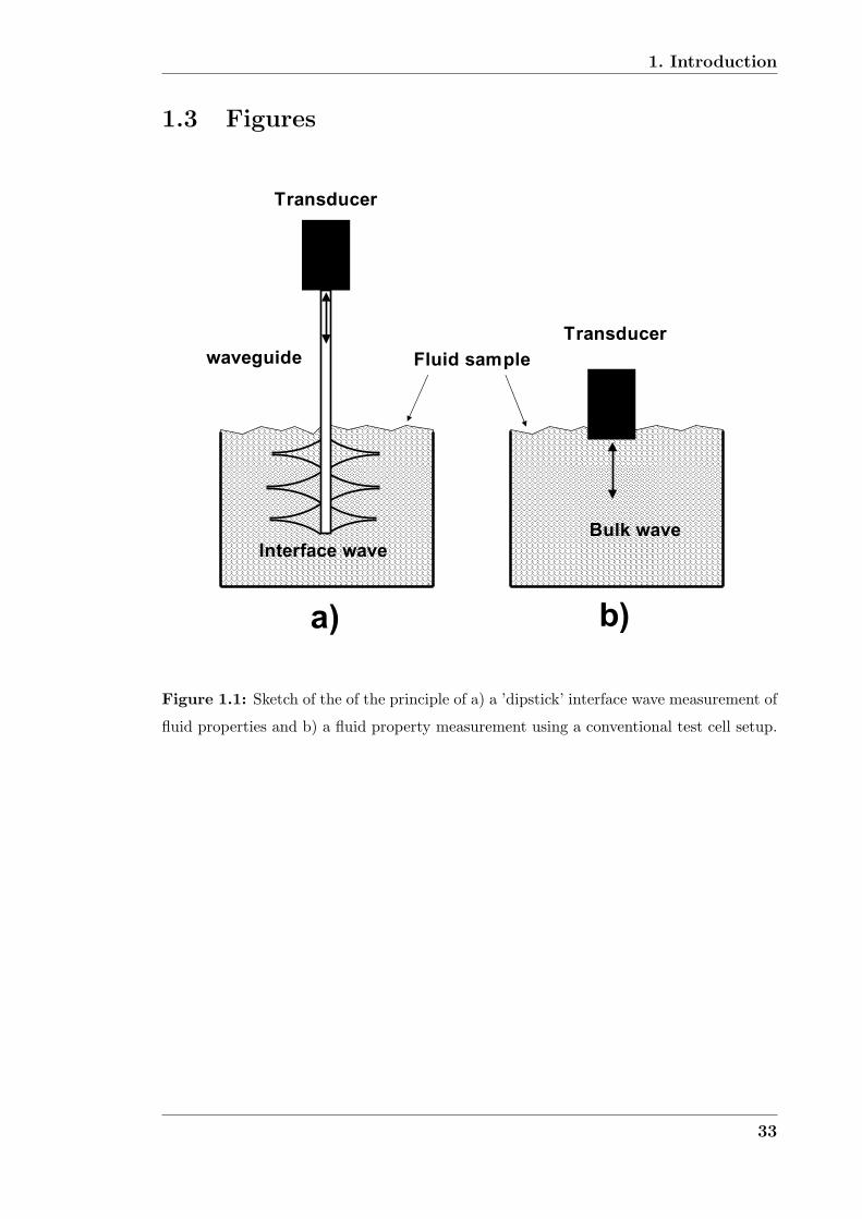
An attractive alternative to test cell based approaches could be the use of a guided
ultrasonic interface wave to measure the fluid properties. In this thesis the use
of the quasi-Scholte mode for fluid property measurements was investigated. The
quasi-Scholte mode is an ultrasonic interface wave trapped at the surfaces of a plate
that is immersed in a liquid. It resembles the Scholte wave on a single boundary
between a solid and a liquid. A large proportion of the energy of the interface wave
is travelling in the liquid which makes it very sensitive to the fluid properties. The
energy contained within the wave decays with distance from the interface so that the
energy is localised at the interface between solid and liquid or plate and liquid for
the quasi-Scholte mode. The waveguide therefore determines the geometry of the
problem completely which removes diffraction or beam spreading issues. It is also
possible to separate the transducer location from the sensing area which potentially
enables measurements at high temperatures and in harsh environments. A sketch
illustrating the principle of the ’dipstick’ interface wave measurement and the con-
ventional test cell based measurement of fluid properties is shown in figure 1.1.
The dipstick separates the transducer from the test region and so allows measure-
ments to be taken in conditions that the transducer itself cannot tolerate. This
concept has other applications and one of them is thickness gauging at high tem-
peratures which is addressed in the second part of this thesis.
Whilst thickness monitoring is a routine task at room temperature, standard equip-
ment fails at elevated temperatures (> 300◦C) and when exposed to high radiation
levels. This is mainly due to depolarisation of the piezo-electric transducer materials
at temperatures above the Curie point and under the influence of radiation. Current
research is being carried out to find more robust transducer materials that work at
extreme conditions [4], [5], however the development and production of these mate-
rials is expensive which makes them currently comparable to expensive alternative
techniques such as laser ultrasonics. Therefore the use of a buffer waveguide system
for structural monitoring in harsh environments is very attractive. It allows the
use of standard ultrasonic equipment to excite and receive ultrasonic signals at a
waveguide end that is located in a safe environment while the testing is carried out
29
1. Introduction
at the other waveguide end under extreme conditions.
Potential applications of the buffer waveguide in power plants, petro chemical plants
or general processing plants with the benefit of reducing shut down times can be
envisaged. An ’acoustic cable’ would be installed after subcritical wall thinning
due to erosion or corrosion has been found in a plant component during a routine
non-destructive testing check up. Instead of prolonging the shut down of the plant
to wait for replacement components, the plant could be restarted immediately and
the condition of the feature of concern can be monitored. In case the component
reaches a critical condition an emergency shut down could be carried out, however
it is more likely that the critical part would survive until the next scheduled shut
down for which an effective replacement can be planned. The monitoring of erosion
or corrosion of pipe walls, boiler components or elbow sections is thus possible.
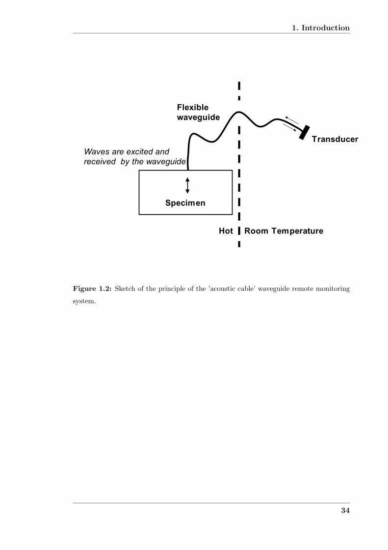
The development of a robust waveguide and the optimisation of the wave propaga-
tion therein was carried out. The geometry of the waveguide and the polarisation
of the wave in the waveguide were also investigated in order to find a waveguide
that can simultaneously act as source and receiver of bulk waves on a test piece. A
sketch of the principle of the waveguide monitoring system is shown in figure 1.2.
1.2 Thesis outline
Following this outline, in chapter 2 a brief review of basic wave propagation in bulk
media is presented. The main principles and mathematical expressions for bulk
waves are given. Then guided waves, which result from a superposition of reflec-
tions of bulk waves at boundaries, are introduced. A section in the chapter also
summarises existing guided wave material property measurement techniques before
the chapter closes with a brief overview of ultrasonic spectrometry.
The theoretical modelling of the quasi-Scholte mode is the subject of chapter 3.
30
1. Introduction
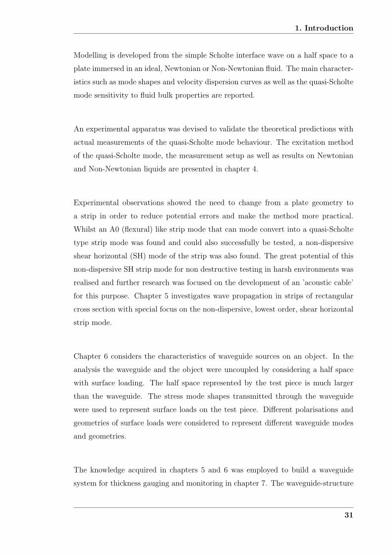
Modelling is developed from the simple Scholte interface wave on a half space to a
plate immersed in an ideal, Newtonian or Non-Newtonian fluid. The main character-
istics such as mode shapes and velocity dispersion curves as well as the quasi-Scholte
mode sensitivity to fluid bulk properties are reported.
An experimental apparatus was devised to validate the theoretical predictions with
actual measurements of the quasi-Scholte mode behaviour. The excitation method
of the quasi-Scholte mode, the measurement setup as well as results on Newtonian
and Non-Newtonian liquids are presented in chapter 4.
Experimental observations showed the need to change from a plate geometry to
a strip in order to reduce potential errors and make the method more practical.
Whilst an A0 (flexural) like strip mode that can mode convert into a quasi-Scholte
type strip mode was found and could also successfully be tested, a non-dispersive
shear horizontal (SH) mode of the strip was also found. The great potential of this
non-dispersive SH strip mode for non destructive testing in harsh environments was
realised and further research was focused on the development of an ’acoustic cable’
for this purpose. Chapter 5 investigates wave propagation in strips of rectangular
cross section with special focus on the non-dispersive, lowest order, shear horizontal
strip mode.
Chapter 6 considers the characteristics of waveguide sources on an object. In the
analysis the waveguide and the object were uncoupled by considering a half space
with surface loading. The half space represented by the test piece is much larger
than the waveguide. The stress mode shapes transmitted through the waveguide
were used to represent surface loads on the test piece. Different polarisations and
geometries of surface loads were considered to represent different waveguide modes
and geometries.
The knowledge acquired in chapters 5 and 6 was employed to build a waveguide
system for thickness gauging and monitoring in chapter 7. The waveguide-structure
31
1. Introduction
joint is the most critical part of the assembly and several joining methods from
manual coupling with shear couplant via clamping to permanent attachment by
means of welding or soldering were investigated. A prototype was built and thick-
ness measurements on a calibration block at room temperature as well as thickness
monitoring at 500◦C for long periods (> 1 month) were carried out.
Chapter 8 summarises the main findings of this thesis and indicates future work and
improvements for both techniques. Some of the work on the quasi-Scholte mode has
been published. A list of these publications is given at the end of the thesis after
the references section.
32
1. Introduction
1.3 Figures
��������
��������
��� ���
�������������������
�����������
�� ��
Figure 1.1: Sketch of the of the principle of a) a ’dipstick’ interface wave measurement of
fluid properties and b) a fluid property measurement using a conventional test cell setup.
33
1. Introduction
��������
��� ���
���������
������� �
�������������� ��� �
������ ���������������� �
��� �������������
Figure 1.2: Sketch of the principle of the ’acoustic cable’ waveguide remote monitoring
system.
34
Chapter 2
Basic principles of bulk and
guided waves
2.1 Wave propagation in bulk media
The propagation of elastic waves in infinite isotropic media has gained a lot of atten-
tion in the literature. There are many texts that describe the underlying principles
[6], [7], [8], [9]. Therefore here only a short introduction to the underlying equations
will be given. Starting in a Cartesian coordinate system the general equation of
motion is given by:
ρ∂2u
∂t2= ∇σ (2.1)
where ρ is the density of the medium, u is the displacement and σ the stress field
tensor in the medium. ∇ is the differential operator. It is convenient to introduce
Hooke’s law to relate stresses to strains and displacements.
σij = λδijεkk + 2μεij (2.2)
εij =1
2(∂ui
∂xj
+∂uj
∂xi
) (2.3)
35
2. Basic principles of bulk and guided waves
By substituting equations 2.2 and 2.3 into equation 2.1 the Navier equation is ob-
tained.
ρ∂2u
∂t2= (λ + μ)
∂
∂xi
∂uj
∂xj
+ μ∂2ui
∂x2j
(2.4)
which may be expressed in vector form:
ρu = (λ + μ)∇(∇.u) + μ∇2u (2.5)
By means of the Helmholtz decomposition the displacement field can be separated
into a scalar (φ) and vector (H) potential [10].
u = ∇φ + ∇× H (2.6)
In combination with equation 2.5 after some algebra the following expression is
obtained:
∇[ρ∂2φ
∂t2− (λ + 2μ)∇φ2] + ∇× [ρ
∂2φ
∂t2− μ∇2H] = 0 (2.7)
Thus equation 2.7 can be split into two independent equations; one for the dilata-
tional or equivoluminable (φ) motion and one for rotational (H) motion.
∂2φ
∂t2= c2
l ∇2φ (2.8)
∂2H
∂t2= c2
s∇2H (2.9)
where
cl =
√λ + 2μ
ρ(2.10)
cs =
√μ
ρ(2.11)
36
2. Basic principles of bulk and guided waves
cl and cs are the velocities of dilatational (longitudinal) and rotational (shear) waves
in the infinite isotropic medium. A general solution to 2.8 and 2.9 can be found by:
φ,H = Aei(kl,sx−ωt) (2.12)
with the secular equation
k2l,s =
ω2
c2l,s
(2.13)
where x is the spatial coordinate of the wave, t is the time variable, A is an arbitrary
wave amplitude, ω is the angular frequency, cl and cs are the longitudinal and shear
wave velocities respectively and kl and ks are the corresponding wavenumbers. The
secular equation links the wavenumber of the wave to the velocity of the wave. In
general the wavenumber is a complex vector:
k = n · kre + ib · kim (2.14)
where n and b are the unit vectors defining the directions of kre and kim respectively.
Substituting this into 2.12 yields the following description of a wave:
φ = Aei(n·krex+ib·kimx−ωt) = Aei(n·krex−ωt)e−b·kimx (2.15)
This clearly shows that the harmonic oscillatory term in time and space remains with
kre as characteristic wavenumber, while the imaginary component of the wavenumber
kim simply adds an exponential decay. Thus the phase velocity of a wave is defined
by the real part of the wavenumber
cph =ω
kre
(2.16)
and the attenuation is described by the imaginary component of the wavenumber
kim.
37
2. Basic principles of bulk and guided waves
The secular equation for a complex wavenumber is the following:
ω2
c2= k2
re − k2im + i2krekim(n · b) (2.17)
For an elastic wave the phase velocity is purely real. This results two conditions for
the complex secular equation 2.17. Either kim = 0 which describes the propagation
of homogeneous plane waves, or kim �= 0 but (n · b) = 0 which describes an inhomo-
geneous wave whose attenuation vector kim is normal to the propagation direction.
Both waves travel unattenuated in the direction of their phase. Examples of inho-
mogeneous waves in liquids are Scholte and Rayleigh waves, while leaky Lamb waves
are an example of inhomogeneous waves with attenuation in the direction of travel
[11], [12].
The above analysis can be extended to viscoelastic materials. The approach is
well described in the literature ([13], [14], [15]) and hence only the results will be
mentioned here. As for elastic waves the governing equations in the viscoelastic case
can be split up into shear and longitudinal waves with their respective velocities:
cl =
√λ + 2μ
ρ+ i
λ′ + 2μ′
ρ(2.18)
cs =
√μ
ρ+ i
μ′
ρ(2.19)
where cl, cs are the complex longitudinal and shear bulk velocities respectively, ρ is
the density, λ and μ are the real Lame constants and λ′ and μ′ are the imaginary
Lame constants. This time the complex secular equation 2.17 will result in real and
imaginary wavenumber vectors that are non zero and in general n and b are neither
parallel nor perpendicular. In experiments the wave velocity and attenuation of a
material are measured on a parallel propagation path. This measures the phase
velocity along the propagation path and the attenuation (projection of imaginary
wavenumber) in the direction of propagation.
38

2. Basic principles of bulk and guided waves
2.2 Guided Waves
Guided waves are waves that, like light in an optical fibre, are guided along the
structure in which they propagate. Here ’guided wave’ refers to an elasto-dynamic
guided wave rather than any other type of wave. Elasto-dynamic guided waves have
been known since the last century and perhaps the simplest type of guided wave is
the Rayleigh wave [16] that is guided along the interface of an infinite elastic half
space and a vacuum. In contrast to bulk waves that were introduced in section
2.1 a condition for guided waves to develop is the existence of an interface between
two materials. The basic principles of elastic guided waves are very well known and
several textbooks [8], [17], [18] discuss the topic, thus here an extensive treatment
is omitted and only the main characteristics are revised.
In a plate, guided waves are often also called ’Lamb waves’ [19] and can be thought
of as a superposition of shear and longitudinal waves that propagate in the plate
material and get reflected back and forth between the two surfaces of the plate.
The feature that defines a guided wave is, as for waves in general, the complex
wavenumber which is expressed in the plane of the structure along the propagation
direction. The complex wavenumber is generally a function of frequency; its cal-
culation results from the boundary conditions that are imposed at the surfaces of
a waveguide. There are infinitely many solutions to the governing equations which
makes it possible for many guided wave modes to coexist. Each mode has its own
phase velocity-frequency relation and a corresponding mode shape.
A typical dispersion curve for a 1 mm thick steel plate is displayed in figure 2.1.
The curve shows the phase velocity of different modes as a function of frequency.
The phenomenon of a changing phase velocity with frequency is called dispersion,
it results in the distortion of the shape of a multi frequency wave packet that prop-
agates for long distances. This is a very important effect that has to be taken care
of when working with long range guide wave applications [20], [21] (see also section
2.2.1).
39
2. Basic principles of bulk and guided waves
Figure 2.1 also shows different lines; these are the different propagating modes (non
propagating modes are omitted here) which are labelled in the conventional style,
with S and A representing symmetric and antisymmetric modes respectively and
the numbers indicating their harmonic order. The higher the frequency the shorter
is the wavelength of ultrasonic waves and more and more mode solutions exist at
higher frequencies.
In figure 2.1 the phase velocity is plotted against the product of frequency times
thickness. Guided waves are strongly geometry dependent; however for the simple
plate case the dispersion curves can be normalized with respect to thickness by plot-
ting them against the frequency thickness product. For example a 2mm thick plate
at 0.5MHz has the same phase velocity as a 5mm thick plate at 200 kHz.
The dispersion curve in figure 2.1 was obtained using a software tool (DISPERSE
[22]) especially developed for the tracing of dispersion curves in multilayered plate
systems [23] and multilayered cylindrical structures [24]. The software uses the
partial wave technique and represents the waves in each layer by partial longitudinal
and shear waves that leave and enter a layer boundary. On each boundary the
boundary conditions (continuity or fixed values for stresses and displacements) have
to be fulfilled. At each frequency this allows the assembly of a global matrix [25].
The problem results in an eigenvector-eigenvalue problem which can be solved. The
eigenvalues correspond to the wavenumber of a mode while the eigenvectors represent
the mode shape of this particular mode. A solution of the displacement takes the
below form:
U(t) = U(x2)ei(kx1−ωt) (2.20)
where U(x2) is a displacement distribution function (mode shape), k is the wavenum-
ber of the guided wave mode, x1 the propagation direction, x2 the direction normal
to the propagation direction, ω the angular frequency and t the time variable.
The complex wavenumber and mode shape describe a guided wave mode completely.
40
2. Basic principles of bulk and guided waves
However the solutions only describe the modes that can propagate in a free system.
To excite a mode a transducer will have to be attached to the waveguide system.
This modifies the system and supports the excitation of selected modes only. The
excitability function [26] can be used to evaluate the likely mode excitation efficiency
of a transducer for a certain mode at a certain position on the waveguide.
2.2.1 Dispersion
An ultrasonic signal pulse is made up of several frequency components. If the fre-
quency components travel with the same velocity the pulse shape will be conserved
over the whole propagation path. However if the frequency components travel at
different velocities, they will disperse out with propagation distance from the source.
This makes the original signal shape longer and less strong in amplitude. Figure
2.2 shows a 5 cycle 500 kHz Hanning windowed A0 mode (steel plate 1mm) signal
at excitation and after a propagation path of 0.5 m. The dispersion in form of a
change in signal shape is clearly noticeable. The major frequency components that
are contained within the excitation signal range from 350 to 650 kHz. The A0 mode
is considerably dispersive in this region. The effects of diminished signal amplitude
and increased signal length are both detrimental to ultrasonic techniques and espe-
cially for the purposes of thickness gauging and defect monitoring. The increased
signal length reduces the resolution of the device while the reduced signal amplitude
reduces the propagation range and the signal to noise ratio.
Dispersion however can be corrected for by methods such as described by Wilcox
et al. [27]. Another means of overcoming dispersion effects is the use of time rever-
sal [28]. A signal is sent along the waveguide, it propagates dispersively along the
waveguide and a distorted signal returns to the transducer. The signal is recorded
and then time reversed, i.e. the signal is sent back to front so that the slower trav-
elling parts that arrive later are sent first and faster parts are sent later. The faster
signals catch up with the slower ones so that the received signal is undistorted at
the receiver position. The time reversed signal can either be simulated or measured.
Therefore apart from being another complication, dispersion can be overcome as
41
2. Basic principles of bulk and guided waves
long as a single mode propagates in the waveguide.
2.2.2 Mode shapes
The mode shapes of a mode are the displacement, stress or other related property
variations across the cross section of the waveguide. Figure 2.1 shows that three
propagating modes exist at low frequencies. Theses are the fundamental three plate
waves of compressional, flexural and shear horizontal nature. Figure 2.3 displays
the plate geometry that is considered here, the polarisation directions and sketches
of the three fundamental modes. In the limit of low frequency thickness products
the displacement mode shape of each of the fundamental modes is uniform across
the cross section and in the direction of polarisation (for flexural modes there is a
linear variation of the less strong in-plane displacement across the thickness). At
higher frequency thickness products the mode shape will start to vary across the
cross section (thickness) of the plate. Usually mode shapes are displayed in a plot
displaying the position against the amplitude of displacement or stress component
of the mode. The mode shapes are of arbitrary absolute amplitude but show the
correct relative amplitude compared to another displacement or stress component.
Figure 2.4 shows the mode shapes of the three fundamental modes at a low frequency
thickness product (0.1 MHz mm). Figure 2.5 shows the mode shape of the same fun-
damental modes at higher frequency thickness products. The displacements deviate
considerably from the almost uniform profiles observed at low frequency thicknesses,
except for the SH0 for which the mode shape does not change with frequency.
2.2.3 Wave propagation in rods and wires
Dispersion curves for a rod/wire of 1 mm radius have been traced using the DIS-
PERSE software and are shown in figure 2.6. The naming convention that is shown
in the figure has been adopted after Silk and Bainton [29]. The first letter L,T,F
42
2. Basic principles of bulk and guided waves
stands for longitudinal, torsional and flexural wave. The first number in the bracket
corresponds to the circumferential order of the mode. The circumferential order of
a mode specifies the variation of the mode shape around the circumference of the
structure. For example a circumferential order of 1 indicates that the mode shape
varies sinusoidally around the circumference with one complete sinusoidal cycle. Cir-
cumferential order 2 would vary with 2 complete cycles, order 3 with 3 sinusoidal
cycles and so on. Since torsional and longitudinal waves always are axisymmetric
their first number in the bracket is always zero. The second integer in the bracket
indicates the mode number and differentiates the modes of the same family. There
are an infinite number of circumferential orders and an infinite number of modes
for each of these circumferential orders. Figure 2.6 only displays the axisymmetric
(order 0) and the first circumferential order of flexural waves to avoid crowding the
figure with excessive amounts of data.
The phase velocity dispersion curves of a rod or wire overall show similar character-
istics to those of a plate. The fundamental modes originate from the same velocities
as in the plate case at the low frequency limit (L-Bar velocity, T- shear velocity,
F-0) and asymptote to the same velocities as in the plate case at high frequencies
(L,F-Rayleigh velocity, T-shear velocity). The transition from the low frequency be-
haviour to the high frequency behaviour occurs earlier for rods than in the plate case.
2.3 Existing techniques for material property mea-
surements using waveguides
Guided wave testing has found applications in long range pipe testing [20]. Dur-
ing application in the field it was noted that embedded and coated pipes adversely
affected guided wave propagation. This considerably reduced propagation range of
the waves in the waveguide. The undesirable effect on the wave propagation char-
acteristics led researchers to investigate whether the embedding material properties
could be investigated by the use of guided ultrasonic waves.
43
2. Basic principles of bulk and guided waves
Nagy and co-workers [30], [31] investigated the effect of fluid loading on thin wires.
Kim and Bau [32] and Shepard and Friesel [33] investigated the possibility of density
measurement using guided waves. Vogt et al. [34], [35], [36] thoroughly described
the theory of embedding material property measurements using guided waves. They
measured fluid viscosity using a torsional wave in a wire, they repeated the same
exercise using a longitudinal wave and also evaluated the bulk velocity of the sur-
rounding medium this way. The effect of leakage was used to measure the embedding
material properties. Leakage of energy is caused due to excitation of bulk waves in
the surrounding medium. These bulk waves are set up due to surface displacements
of the waveguide and then radiate away from the waveguide. A torsional wave in a
waveguide (or a shear horziontal wave in a plate see section 3.5) is ideal for viscosity
measurements since it only exhibits rotational/shear displacements at the surface
of the waveguide. This entrains more or less liquid and thus causes more or less
wave attenuation depending on the liquid viscosity. The same effect can be used
with the lowest order compressional L(0, 1) mode of a wire. At higher frequencies
this mode has the additional advantage of mainly exhibiting out-of-plane surface
displacements due to the Poisson effect. At these operational frequencies leakage
is mainly due to leakage of longitudinal waves from the waveguide surface, which
enables the determination of the longitudinal bulk velocity of the fluid.
When the embedding medium is attenuating the guided wave very strongly another
method can also be used. Under these conditions a strong entry reflection of the
guided wave can be noted. Analysis of this entry reflection can also be used to
determine the material properties [36].
However all of the above methods effectively measure the influence of the impedance
of the embedding medium at the surface of the waveguide. None of the energy that
returns to the transducer has actually travelled in the embedding medium. Since
the bulk attenuation of a fluid does not influence its impedance significantly it is
almost impossible to determine the bulk attenuation of an embedding fluid from
those measurements. This issue has been addressed in this thesis. The use of an
44
2. Basic principles of bulk and guided waves
interface wave whose energy travels in the waveguide as well as in the embedding
fluid makes the guided wave measurement sensitive to both velocity and attenuation
of the embedding medium. The guided wave that was used was called the quasi-
Scholte wave due to its similarity to the Scholte wave between two half-spaces that
is commonly seen in geophysics. The Scholte and quasi-Scholte wave theory will be
thoroughly discussed in chapter 3.
2.4 Ultrasonic spectrometry
In ultrasonic spectrometry the velocity and attenuation spectrum of a material are
measured. As in any other spectrometry certain features in the ultrasonic velocity
and attenuation spectrum can be utilised to identify properties of the investigated
material. The simplest example to illustrate this is the determination of density or
modulus from a measured ultrasonic velocity. For ideal fluids the identity cL =√
Kρ
can be used to either deduce the bulk modulus (K) or density (ρ) of the investigated
material once the other is known. In reality materials are not ideal and more specific
data has to be extracted from a sample. The differences in velocity and attenua-
tion spectra help to monitor phase transitions, chrystallisation, melting, freezing,
curing, addition of ingredients and other processes [37]. Ultrasonic spectroscopy is
an important measurement technique especially in the food industry. An important
industrial application of ultrasonic spectrometry is particle sizing [2], [38]. Here the
attenuation caused by scattering from the particles in suspensions or emulsions is
measured and through mathematical models related to particle size [39], [40], [41].
The main advantage of ultrasonic spectrometry is the possibility to examine opaque
samples where standard optical techniques fail. Measurements are also fast and no
prior treatment of the material to be investigated is needed. The principle of the
technique is described below.
The properties of the material to be measured are the ultrasonic velocity and the
attenuation over a wide range of frequencies (typically 0.1− 20 MHz). The velocity
is the distance that an acoustic signal travels per unit time and the attenuation is
the decrease in amplitude of this signal per unit distance. There are several ways to
45

2. Basic principles of bulk and guided waves
measure these quantities, the most common techniques being through-transmission,
pulse echo and interferometry. Schematics of the three techniques are shown in
figure 2.7. In every technique a transducer (E) excites an ultrasonic signal and ei-
ther the same transducer receives the signal (pulse echo, interferometry) or another
transducer (R) is used to pick up the signal (through-transmission). In pulse echo
and through transmission the transducers are accurately mounted and aligned in a
test cell so that the distance between the transducer faces or the transducer and the
back wall is precisely known. Then a sample is placed into the test cell in between
the transducers and a signal is excited at the transducer. From the time between
excitation and reception of the signal the ultrasonic velocity in the sample can be
determined. The attenuation is determined either by comparison of the decrease
in amplitude of the signal in the test sample to the decrease in amplitude of a
sample with known attenuation or by the decrease in amplitude between successive
reverberations of the signal (pulse echo). However for accurate measurements the
reflection coefficient of the walls has to be taken into account. Also beam spreading
and misalignment can lead to errors. To ensure that the velocity and attenuation are
determined at each frequency, either a narrow band toneburst (consisting of many
cycles) is excited at one frequency and the experiment is repeated for each frequency
within the region of interest or a broad band pulse is excited and Fourier transform
techniques are used to extract the velocity and attenuation at each frequency con-
tained within the excitation pulse.
In the interferometer technique, standing waves are produced between a movable
reflector and the fixed transducer in the test cell. When the reflector moves towards
or away from the transducer a series of maxima and minima in received signal
amplitude are detected by the transducer. These maxima and minima are due
to constructive and destructive interference of the standing waves. The distance
between two maxima is equal to half a wavelength and by the identity c = fλ the
velocity of the wave can be deduced. The attenuation is determined by the decrease
in amplitude of successive maxima as the reflector moves further and further away
from the transducer. The main disadvantage of this method is that it has to be
carried out at a single frequency and that it will take a long time to construct a
complete spectrum.
46
2. Basic principles of bulk and guided waves
A disadvantage of all test cell based techniques is the inherent need for a test cell.
Transducers have to be accurately aligned and a test cell is very difficult to integrate
into a reaction vessel. The environment might be very hostile, high temperatures
would disable standard commercially available transducers and stirring devices make
it impossible to install a bulky test cell within a reaction vessel. The overall measured
attenuation in a test cell has to be of the order of 0.5 np/m in order to avoid large
error magnification [42]. This limits the sample size of the test cell and if highly
attenuating materials flow through a test cell this imposes very slow flow rates.
2.4.1 Particle size determination
Particle size determination in emulsions and suspensions is based on comparison
of experimental ultrasonic velocity and attenuation spectra with theoretically pre-
dicted spectra from mathematical models. McClements [37] and Challis et al. [3]
summarise the most important aspects.
Waves propagating in emulsions and suspensions are altered in several ways: a)
waves are scattered and change direction b) waves are attenuated due to different
energy absorbtion mechanisms c) waves that travel through the suspended particles
and scattered waves interfere with the waves that propagated unaltered through the
medium.
The scattering of an ultrasonic wave depends on the wavelength to particle radius ra-
tio. There are three regimes identified. The long wavelength radius regime (λ > R),
the intermediate wavelength radius regime (λ ∼ R) and the short wavelength radius
regime (λ < R). The long wavelength radius regime is the most important as most
ultrasonic measurements fall into this category, here particle sizes are of the order
of 10 micro metres and less. The mechanisms that scatter waves at the particles are
mainly due to differences in thermophysical properties of the embedding material
and the particle. Under the local pressure and temperature oscillations caused by the
passing ultrasonic wave the particles contract or expand and start pulsating. This
scatters wave energy into all different directions (monopole scattering). Differences
in density of the particle and the surrounding fluid will cause oscillatory motion of
the particle (dipole scattering) as the ultrasonic wave passes. All these processes
47
2. Basic principles of bulk and guided waves
are not ideal and absorb energy, thus causing an excess attenuation compared to
the pure fluid. Mathematically there are also different models for highly concen-
trated (multiple scattering) and less concentrated (single scattering) emulsions and
suspensions.
Different theoretical models for wave propagation in fluids containing particles exist
[39], [40], [41] and [43]. In all these models the thermophysical constants of the
contained materials are entered. Since in real life the the size of particles varies
(polydispersity) a distribution function can be entered. The models then predict
a velocity and attenuation frequency spectrum. This spectrum is compared to the
measured data and the parameters for the particle size distribution that best fit to
the mathematical model are determined. Using these methods particle sizes in the
range from 0.01 to 30 micro meters can be analysed. If the intermediate wavelength
radius regime is also used the whole particle size range can be covered [37]. Par-
ticle sizing is a very well developed specialist field in which very advanced models
and accurate measurements setups are used. Several commercial ultrasonic parti-
cle anlaysers exist currently (Opus [Sympatec GmbH, Germany],Ultrasizer [Malvern
Instruments Ltd.,UK] and DT-1200 [Dispersion Technology,USA]).
2.5 Summary
In this background chapter the basics of ultrasonic wave propagation in unbounded
media were presented. Then the basic characteristics of guided waves were recalled
and references to modelling techniques including the global matrix method were
given. Existing guided wave material property measurements rely on the attenua-
tion due to leakage or the analysis of an entry reflection to characterise the material.
Both leakage and the entry reflection are insensitive to the bulk attenuation of an
embedding fluid. However for fluid characterisation the bulk wave attenuation can
be very important as for example for the application of particle size determination.
The bulk velocity and attenuation measurement of a sample as usually determined
in ultrasonic spectrometry is a very powerful tool to monitor industrial processes.
Ultrasonic measurement technology is well developed in the form of test cells, which
however possess inherent short comings. In the following chapters the development
48
2. Basic principles of bulk and guided waves
of a guided wave ”dipstick” sensor is described. The sensor is measuring the same
ultrasonic velocity and attenuation spectra as the conventional test cell based tech-
niques (see section 2.4), however it removes the need of a test cell with its short
comings and consists solely of a waveguide that is immersed in the sample fluid.
49

2. Basic principles of bulk and guided waves
2.6 Figures
Figure 2.1: Phase velocity dispersion curves for a steel plate: Compressional modes (—),
Flexural modes (- - -) and Shear Horizontal modes (· · ·)
50

2. Basic principles of bulk and guided waves
Figure 2.2: 5 cycle Hanning windowed excitation signal (a) and a prediction by the
DISPERSE [22] software of the signal after 0.5m propagation distance as A0 mode on a
1mm thick steel plate (b)
51
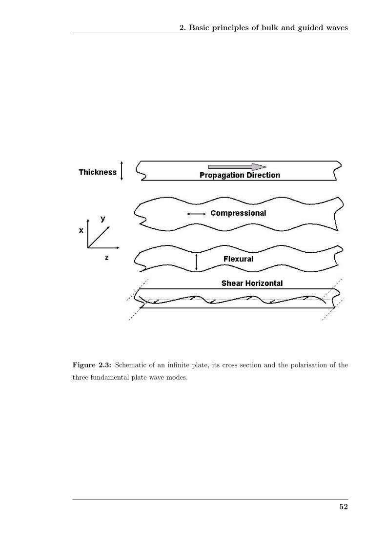
2. Basic principles of bulk and guided waves
Figure 2.3: Schematic of an infinite plate, its cross section and the polarisation of the
three fundamental plate wave modes.
52

2. Basic principles of bulk and guided waves
-1 -0.5 0 0.5 1-0.5
0
0.5
magnitude (arb. units)
p
os
itio
n (
mm
)
a)
-1 -0.5 0 0.5 1-0.5
0
0.5
magnitude (arb. units)
p
os
itio
n (
mm
)
b)
-1 -0.5 0 0.5 1-0.5
0
0.5
magnitude (arb. units)
p
os
itio
n (
mm
)
c)
Figure 2.4: Mode shapes of the (a) S0 mode, (b) A0 mode and (c) SH0 mode at
frequency thickness 0.1 MHz mm of a steel plate. (—) in-plane (z direction) displacement,
(- - -) out-of-plane (x direction) displacement, (· · ·) in-plane (y direction) displacement
53
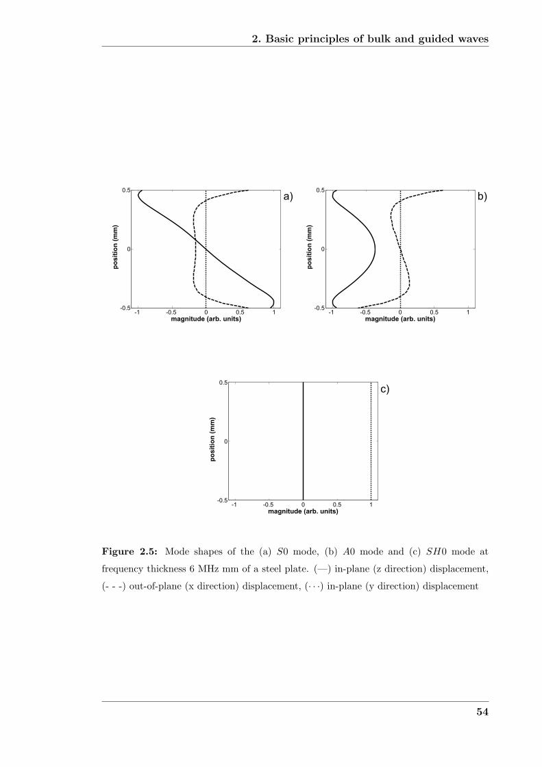
2. Basic principles of bulk and guided waves
-1 -0.5 0 0.5 1-0.5
0
0.5
magnitude (arb. units)
p
os
itio
n (
mm
)
a)
-1 -0.5 0 0.5 1-0.5
0
0.5
magnitude (arb. units)
p
os
itio
n (
mm
)
b)
-1 -0.5 0 0.5 1-0.5
0
0.5
magnitude (arb. units)
p
os
itio
n (
mm
)
c)
Figure 2.5: Mode shapes of the (a) S0 mode, (b) A0 mode and (c) SH0 mode at
frequency thickness 6 MHz mm of a steel plate. (—) in-plane (z direction) displacement,
(- - -) out-of-plane (x direction) displacement, (· · ·) in-plane (y direction) displacement
54
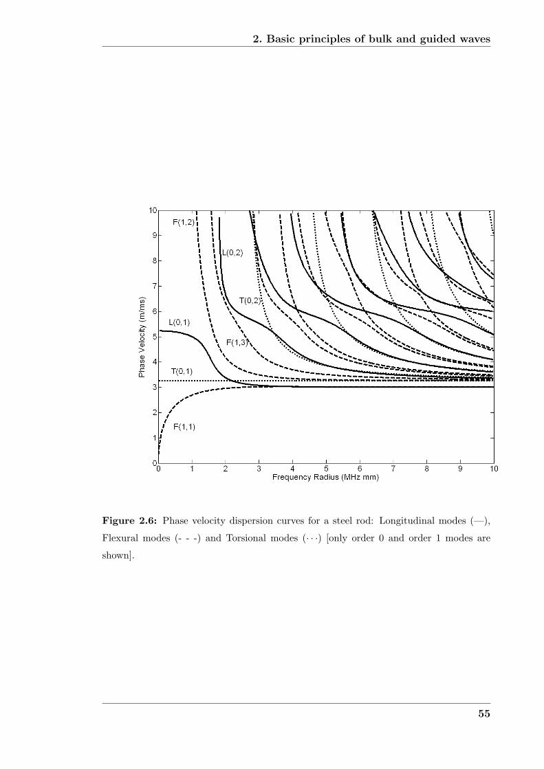
2. Basic principles of bulk and guided waves
Figure 2.6: Phase velocity dispersion curves for a steel rod: Longitudinal modes (—),
Flexural modes (- - -) and Torsional modes (· · ·) [only order 0 and order 1 modes are
shown].
55
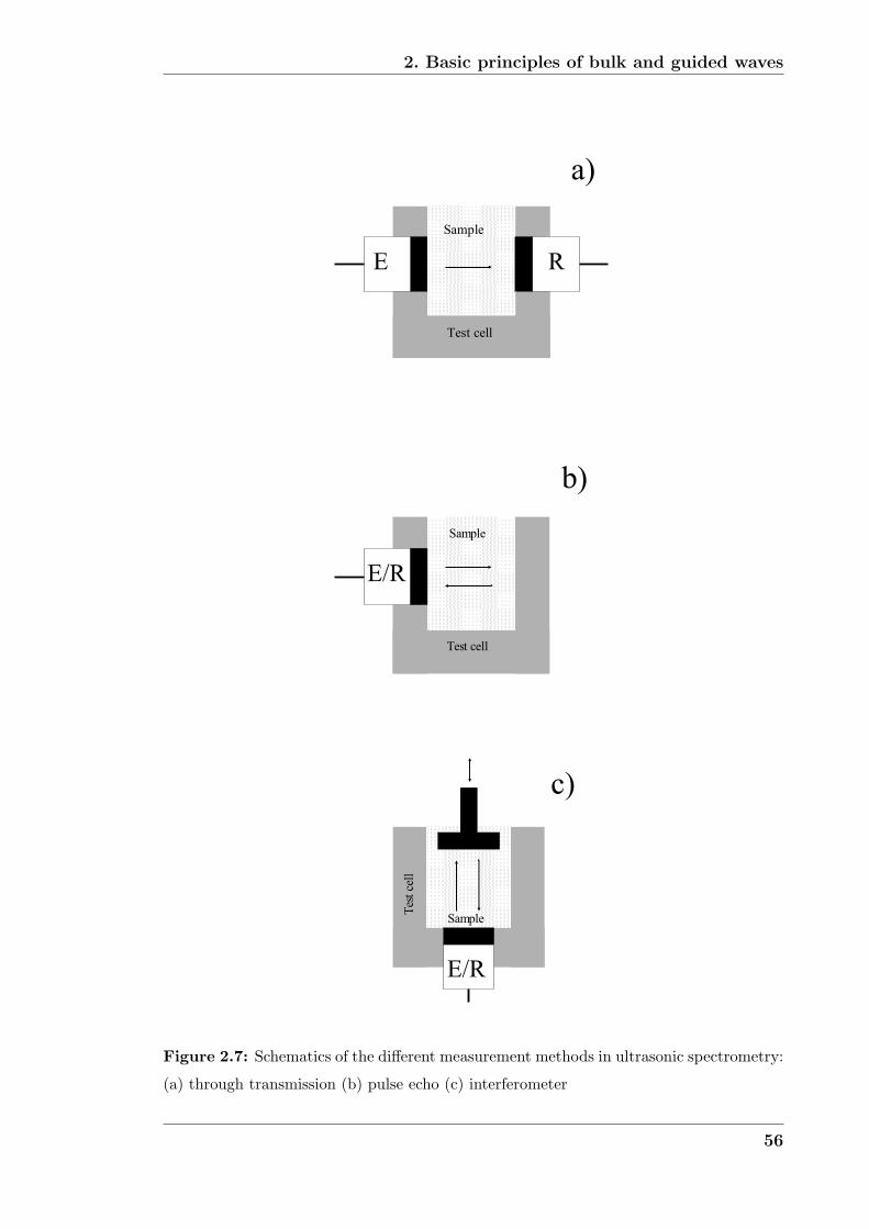
2. Basic principles of bulk and guided waves
� �
� �
����
�� ��
��
� �
���
�����
��� ��
��
� �
���
�����
��� ��
�
Figure 2.7: Schematics of the different measurement methods in ultrasonic spectrometry:
(a) through transmission (b) pulse echo (c) interferometer
56
Chapter 3
Scholte mode and Quasi-Scholte
mode Theory
3.1 The Scholte wave
At the interface of a liquid and solid there exist two propagating solutions to the
governing equation: the leaky Rayleigh wave and the Stoneley-Scholte wave [44].
This thesis focuses on the latter and will for the sake of clarity refer to it as the
Scholte wave. The Scholte wave is a special case of a Stoneley wave (on a solid/liquid
interface) which was first pointed out by Scholte [45]. Subsequently the wave gained
a lot of interest and work on it was extended and revised by many other authors;
Pilant [46], Volkenstein and Levin [47], Padilla et al. [48], Glorieux et al. [44]
and Meegan et al. [49] have extensively modelled the Scholte interface wave on a
boundary between two half-spaces.
For the Scholte wave to exist an interface system of an elastic solid half-space coupled
to a liquid half-space is required. A sketch of such a system can be seen in figure 3.1.
The interface wave will propagate energy along the path described by the interface,
as long as any curvature effects of the interface are large compared to the wavelength
of the wave. The wave energy of the Scholte wave is distributed over both materials,
the solid and the liquid, depending on the material properties of both half-spaces.
For the purposes of fluid characterisation which is discussed in this thesis a high
57
3. Scholte mode and Quasi-Scholte mode Theory
energy content in the fluid is desirable; while in geophysics for the characterisation
of marine sediment a high energy content in the solid is more desirable. The mode
shape of the Scholte wave on a Steel/Water interface is shown in figure 3.2.
Figure 3.2 illustrates that the displacements amplitudes for the Steel/Water inter-
face are extremely large in the liquid compared to the solid. The polarisation of the
displacement is also mostly parallel to the interface with a small component of out-
of-plane displacement. The wave amplitude decays in an exponential manner with
distance from the interface and is unnoticeable at distances far from the interface.
The extent to which the wave penetrates into the fluid depends on the frequency;
at low frequencies the wave penetrates further into the liquid than at high frequen-
cies. The Scholte wave in this special case can thus roughly be approximated by
a longitudinal bulk wave that travels along the interface but decays away from the
interface. It is therefore ideal for fluid property measurements.
3.2 Theoretical modelling of the Scholte wave
The properties of an interface wave can be theoretically modelled using the par-
tial wave technique as described in references [8] and [23]. Recall the sketch of
the interface wave system shown in figure 3.1. The displacements and stresses in
the system are determined by combining the general solution of the displacements
and stresses in each material with the system boundary conditions (continuity of
stresses and displacements across the interface and no incoming partial waves). Af-
ter some algebra the system of equations can be expressed in matrix form as follows:
⎡⎢⎢⎢⎢⎢⎣
−(1 + β21) −2β1 (1 + β2
2)g −2β2g
2α1 (1 + β21) 2α2g −(1 + β2
2)g
1 β1 −1 β2
−α1 −1 −α2 1
⎤⎥⎥⎥⎥⎥⎦ ·
⎛⎜⎜⎜⎜⎜⎝
L1
T1
L2
T2
⎞⎟⎟⎟⎟⎟⎠ = 0 (3.1)
where L1 and L2 are the amplitudes of the longitudinal partial waves in materials
1 and 2 respectively; T1 and T2 are the corresponding shear partial waves. The
remaining parameters in the equation are defined by:
58
3. Scholte mode and Quasi-Scholte mode Theory
α2n = 1 − c2
C2ln
(3.2)
β2n = 1 − c2
C2tn
(3.3)
g =G2
G1
(3.4)
where n = 1, 2 represent the materials; Cl represents the longitudinal velocity and
Ct the transverse velocity; G1 and G2 are the shear moduli of the materials.
In order for a non trivial solution to exist, the determinant of the term in square
brackets in equation 3.1 has to equal zero. In the case of an interface between an
ideal fluid (G1 = 0) and an elastic solid the matrix equation reduces to:
⎡⎢⎢⎣
iρfc2l (1 + β2
2)G2 −2β2G2
0 2α2G2 −(1 + β22)G2
α1 iα2 −i
⎤⎥⎥⎦ ·
⎛⎜⎜⎝
L1
L2
T2
⎞⎟⎟⎠ = 0 (3.5)
After some algebra this results in the characteristic equation for a Scholte wave [8]:
[2 −
(c
ct2
)2]2
−4
√1 −
(c
ct2
)2√
1 −(
c
cl2
)2
−iρl
ρs
[cl
cl2
√c2l2 − c2√
c2 − c2l c
4t2
]= 0(3.6)
where cl is the liquid bulk velocity, ρl is the liquid density, cl2 is the solid longitu-
dinal bulk velocity, ct2 is the solid transverse bulk velocity, ρs is the solid density
and c is the Scholte wave velocity. This expression yields the phase velocity (or
wavenumber) - frequency relationship that describes the mode. In this special case
of a wave propagating along the interface of an elastic solid and an ideal fluid the
mode is non dispersive, i.e. the phase velocity does not change with frequency.
59
3. Scholte mode and Quasi-Scholte mode Theory
By substituting the calculated phase velocity into equation 1 and fixing the am-
plitude of one partial wave at unity the mode shape of the Scholte wave can be
evaluated [23]. Figure 3.2 shows the mode shape of a Scholte wave on a steel-water
interface.
3.2.1 Influence of material properties on the Scholte wave
The theoretical description of the Scholte wave has been thoroughly investigated
by many researchers ([44],[47],[50]). It can be shown that the phase velocity of the
Scholte wave is limited by the lower of the fluid or the transverse bulk velocity of the
elastic medium (cscholte < cliquid, ct,solid). The dependence of the Scholte wave veloc-
ity on the density and longitudinal velocity ratio of the neighbouring materials can
be displayed on a contour map as shown in figure 3.3. The Scholte wave velocity is
close to the fluid velocity when the solid material is very stiff and dense. As the stiff-
ness of the solid compared to the fluid reduces, which is indicated by moving upward
on the ordinate in figure 3.3, the Scholte velocity decreases. Also by reducing the
solid density the Scholte velocity is reduced (movement to the right on the abscissa).
The distribution of the fraction of energy flowing in the fluid and solid also depends
on the density ratio of the two materials. A similar contour map to that of figure
3.3 has been created to visualise the distribution of energy flow in the two materials.
Figure 3.4 shows the fraction of the total energy flow that is located in the liquid
for different density and longitudinal velocity ratios of the two media.
The contour maps of the Scholte wave velocity and energy distribution in figure 3.3
and 3.4 have been plotted for a fixed value of Poisson’s ratio, which in this case was
0.2865 and corresponds to a material like steel. The analysis can be carried out for
other Poisson’s ratios which will slightly alter the contour maps. The availability
and affordability of steel made it the material of choice and hence its Poisson’s ratio
was chosen for the contour maps.
60
3. Scholte mode and Quasi-Scholte mode Theory
3.2.2 Modelling a viscous fluid
The derivation of the properties of the Scholte mode for an ideal fluid has been dealt
with above. The derivation for a viscous fluid uses a similar approach. Here the
fluid is assumed to be Newtonian. The viscous medium is modelled as a solid with
appropriate parameters. More theoretical details on this approach are described in
[22], [30]. The following equations representing the viscous fluid can be deduced:
Cl =
(λf
ρ
)1/2
(3.7)
κl =
(4πων
3C2l
)(3.8)
Cs = (2ων)1/2 (3.9)
κs = 2π (3.10)
where Cl is the longitudinal bulk wave velocity, λf is the fluid bulk modulus. κl
is the longitudinal bulk wave attenuation (nepers per wavelength), ω the angular
frequency and ν the kinematic viscosity of the fluid. Cs stands for the shear bulk
wave velocity and κs for the shear bulk wave attenuation (nepers per wavelength).
Equations 3.7-3.10 assume low viscosities which introduces some simplifications in
their derivations [22].
In order to solve for the viscous Scholte equation the complex bulk velocities and
moduli have to be entered into equations 3.2-3.4. These are found from equations
3.7-3.10 by the following expression:
cln =Cl
1 + iκlCl
ω
(3.11)
ctn =Cs
1 + iκsCs
ω
(3.12)
61
3. Scholte mode and Quasi-Scholte mode Theory
g =G2
−iωρlν(3.13)
where cln is the complex longitudinal bulk velocity of material n and ctn is the com-
plex transverse bulk velocity of material n.
By substituting the above equations into equations 3.2-3.4 where applicable, a new
characteristic equation and mode shape can be found. The Scholte wave in this sys-
tem becomes dispersive and attenuated. However the dispersion effect is relatively
weak and for small viscosities the map in figure 3.3 still accurately represents the
velocity and density dependence. The model can also easily be extended to non-
viscous fluids as long as the quantities cln and ctn of equations 3.11 to 3.13 can be
determined, for example by means of another model or direct measurement.
3.3 Properties of the quasi-Scholte plate mode
In real life it is impossible to find a semi-infinite half-space; a very thick piece
of solid material would have to be used which would be inconvenient to handle.
Therefore another boundary was introduced to the system. This creates a plate
that is immersed in an infinite (in practice large) space of liquid. In this new fluid-
plate system a mode that is very similar to the Scholte wave exists. The mode was
termed quasi-Scholte (QS) mode, because it asymptotically approaches the Scholte
wave velocity at high frequencies. In the following section the quasi-Scholte mode
will be examined in more detail. A software package called DISPERSE [22] was
used to trace the dispersion curves. DISPERSE is a multi purpose package to trace
dispersion curves in multiple material layer stacks of solid materials and viscous
fluids. Also a routine solely for the purpose of tracing the quasi-Scholte mode
dispersion curves was written in Matlab and the basic equations behind the routine
are outlined in Appendix A. It was verified that both programs yield the same
results.
Here the DISPERSE solutions for an embedded plate mode are shown and discussed.
First an inviscid fluid is used as the embedding medium and then a viscous liquid.
62

3. Scholte mode and Quasi-Scholte mode Theory
The velocity dispersion characteristics are virtually unchanged by the introduction of
viscosity but the attenuation is noticeably affected. A steel plate (cl = 5959.5m/s,
cs = 3260m/s, ρsteel = 7932kg/m3, thickness=1 mm) is embedded in an infinite
space of water (cl = 1500m/s, ρwater = 1000kg/m3). Figure 3.5 shows the phase
velocity dispersion curve of the plate Scholte mode. The phase velocity of the quasi-
Scholte plate mode rises with frequency from zero and gradually asymptotes to the
non-dispersive Scholte wave velocity of two elastic half spaces. A physical explana-
tion of the asymptotic behaviour is the decrease of mode wavelength with increasing
frequency. At a certain point the wavelength will be small compared to the thickness
of the plate. Since the Scholte wave displacements decay in an exponential manner
away from the interface the mode resembles a mode on an infinite halfspace at high
frequencies, whereas at lower frequencies the two interfaces of the plate interact.
The phenomenon is also well known in plate waves where the A0 and S0 modes are
asymptotic to the Rayleigh wave solution [51]. In the remainder of this thesis the
plate Scholte mode will be referred to as the quasi-Scholte (QS) mode, the termi-
nology being similar to that of a quasi-Rayleigh wave on a finite plate.
The similarities of the quasi-Scholte mode and the A0 mode in a free plate are high-
lighted by their mode shapes. Figure 3.6(a) shows that the out of plane displacement
component at 100kHzmm is almost constant across the section of the plate and the
strain energy density indicates that most of the energy is propagating in the plate.
At higher frequencies most of the energy is travelling in the fluid as shown in figure
3.6(b). Figure 3.6(c) shows the mode shape in the plate only at 2MHzmm. Dis-
placements decay away from the surfaces and are a minimum at the centre of the
plate. This illustrates the effect of the quasi-Scholte mode becoming asymptotic to
an interface wave (Scholte wave) at high frequencies as discussed above.
An important property of the quasi-Scholte mode is its change in energy partition
between fluid and solid with frequency. Figure 3.7 shows the fraction of energy flow
that is situated in the plate and fluid at different frequencies. At low frequencies
(< 500kHzmm) the energy travels predominantly in the plate while at high frequen-
cies (> 1MHzmm) most of the energy travels in the fluid. The cross over point
63
3. Scholte mode and Quasi-Scholte mode Theory
of the two curves occurs at about 400kHzmm for a steel plate embedded in water.
This means that the mode can be made more or less sensitive to the embedding
medium properties. If highly attenuating materials are surrounding the wave guide,
careful frequency selection will allow an appropriate fraction of energy to travel in
the plate so that a reasonable propagation range can be obtained.
The sensitivity of the QS-mode to bulk fluid properties is demonstrated best by
graphs that plot QS-mode dispersion curves for different properties of the embed-
ding fluid. Figure 3.8 shows the quasi-Scholte mode group velocity as a function
of frequency for different longitudinal velocities of the embedding fluid. Figure 3.9
displays the theoretical attenuation of the quasi-Scholte mode as a function of fre-
quency for different viscosities at a fixed longitudinal bulk velocity of the embedding
medium. A more detailed treatment of the QS-mode sensitivity to fluid properties
can be found in section 3.4.
There are two attenuation mechanisms for the quasi-Scholte and Scholte modes. The
first is the leakage of shear waves from the plate surface into the embedding viscous
fluid and the second is the attenuation of a longitudinal bulk wave in the viscous
fluid. Energy that is guided along the interface in the form of an evanescent longi-
tudinal wave will be attenuated by longitudinal attenuation. In the case of a purely
Newtonian viscous fluid this attenuation is due to viscosity and can be modelled by
equation 3.8 (assuming low viscosities [31]). Also for Newtonian fluids both attenu-
ation mechanisms depend on the viscosity only (see equations 3.8,3.9,3.10). At low
frequencies the shear leakage is dominant while at higher frequencies the evanescent
longitudinal wave attenuation contributes significantly to the quasi-Scholte mode
attenuation. Figure 3.10 shows the total attenuation of the quasi-Scholte mode on
an aluminium plate (cl = 6320.0m/s, cs = 3130m/s, ρal = 2700kg/m3, thickness=1
mm) immersed in glycerol (cl = 1860m/s, ρglycerol = 1258kg/m3 ηglycerol = 1Pas).
A line showing the attenuation due to shear leakage only is also shown (the lines are
traced in DISPERSE; for the shear leakage only case the longitudinal attenuation is
set to κl = 0 in equation 3.8) . The difference between the two curves is linked to the
longitudinal bulk attenuation of the fluid. Thus if the longitudinal bulk velocity and
64
3. Scholte mode and Quasi-Scholte mode Theory
the shear properties of the fluid are known, it is possible to measure the longitudinal
bulk attenuation of the fluid surrounding the waveguide.
Figure 3.10 considers a viscous liquid. The shear properties of the liquid are de-
scribed by equations 3.9, 3.10. Therefore the longitudinal attenuation and the shear
velocity of the embedding medium are both functions of viscosity and frequency.
This has the effect that the quasi-Scholte mode attenuation is almost entirely de-
pendent on the viscosity of the fluid. The phrase ”almost entirely dependent” is
used here since the longitudinal bulk velocity of the fluid has a small effect on the
QS-mode attenuation and the viscosity has a small effect on the group velocity
of the QS-mode. The group velocity of the QS-mode changes by about 10 m/s
(∼ 0.5% of Cl) when the viscosity changes from 0 to 1 Pas for a glycerol-like fluid
(cl = 1860m/s, ρglycerol = 1258kg/m3 ηglycerol = 1Pas). For a Newtonian viscous
fluid the quasi-Scholte mode group velocity is almost entirely dependent on the fluid
bulk velocity and its attenuation is almost entirely dependent on the fluid viscosity.
It can therefore be concluded that a measurement of the QS mode group velocity
and its attenuation can be used to determine the fluid bulk velocity and viscosity.
The assumption of a Newtonian viscous fluid links the bulk shear velocity and bulk
longitudinal attenuation of the fluid to the viscosity; they therefore are not in-
dependent properties. However for a more complex non-Newtonian fluid, the at-
tenuation and viscosity become two independent fluid properties. Therefore for a
non-Newtonian fluid the quasi-Scholte mode attenuation will also not solely depend
on viscosity but also on the fluid bulk attenuation. This is illustrated in figure
3.11, where the QS-mode attenuation is plotted for a liquid of the same viscosity
but with different longitudinal bulk wave attenuation. In order to extract the fluid
bulk attenuation using the QS-mode it is therefore necessary to know the fluid shear
properties or in other words its complex shear velocity. This can be done using a
method such as that described by Vogt [36]. He used a torsional wave in a rod
that is immersed in a viscous fluid. By evaluating the attenuation of the wave, the
shear leakage and thus shear properties of the fluid were determined. The use of a
torsional wave in a rod is physically analogous to a SH-wave in a plate. The latter
was used for the work presented in this thesis since the quasi-Scholte mode also
65
3. Scholte mode and Quasi-Scholte mode Theory
propagates in a plate geometry and therefore the same plate can be used to carry
out a different measurement. Section 3.5 describes the use of the fundamental SH0
mode in a plate to extract the fluid shear properties.
3.4 Quasi-Scholte mode sensitivity to fluid prop-
erties
This section investigates the sensitivity of the quasi-Scholte mode to the fluid bulk
properties. The sensitivity indicates the change in measured property due to a
change in the actual fluid bulk property. Here the sensitivity is defined as:
S =∂M
∂P(3.14)
where S is the sensitivity, M the measured quantity and P the fluid property that
is changing. It is important to know the sensitivity of a measurement technique
in order to identify how accurate it can be and how different sources of error can
influence the measurement. The quasi-Scholte mode is influenced by all the bulk
properties of the fluid, namely bulk velocity, viscosity and bulk attenuation; while
each of these properties simultaneously affect the quasi-Scholte mode, one property
is isolated, this property is then changed and the effect on the measured quantity is
predicted.
3.4.1 Sensitivity to the fluid bulk velocity
For bulk velocity measurements of fluids using the quasi-Scholte mode, the group
velocity or phase velocity of the quasi-Scholte mode can be identified as the measured
quantity and the bulk velocity as the measurand, the property to be measured. The
sensitivity of the quasi-Scholte mode to the fluid bulk velocity thus can be defined
as:
SBvel =∂CQS
∂CB
(3.15)
66
3. Scholte mode and Quasi-Scholte mode Theory
where SBvel is the sensitivity to the bulk velocity, CQS is the quasi-Scholte mode
velocity, either group or phase velocity and CB is the fluid bulk velocity that sur-
rounds the plate.
The DISPERSE software [22] was used to calculate the quasi-Scholte mode group
and phase velocity dispersion curves for different bulk velocities. Results of the
group and phase velocity sensitivity to the fluid bulk velocity are shown in figure
3.12 and 3.13 respectively.
The sensitivity depends on the properties of the fluid and the plate. Therefore plates
of a different material than steel and fluids with higher or lower bulk velocities than
water will have a different sensitivity of the quasi-Scholte mode velocity to the
fluid bulk velocity. However in practice most liquids are water based and steel
is a cheap and readily available material that is well suited to the application.
Hence sensitivities close to those shown in figures 3.12 and 3.13 will most likely
be encountered. Figures 3.12 and 3.13 also show that the quasi-Scholte mode is
insensitive at frequencies below 0.2 MHz mm. The group velocity is always more
sensitive than the phase velocity and in the frequency thickness range of 0.25 − 0.5
MHz mm the quasi-Scholte mode group velocity is most sensitive to the fluid bulk
velocity. At high frequencies a change in bulk velocity is reflected in a change of
equal magnitude in the group velocity of the quasi-Scholte mode.
3.4.2 Sensitivity to the fluid shear viscosity
For fluid viscosity measurements the attenuation of the quasi-Scholte mode will have
to be used. The definition of sensitivity now becomes the following:
SV isc =∂αScholte
∂ηF
(3.16)
where SV isc is the sensitivity to fluid viscosity, αScholte is the attenuation of the
quasi-Scholte mode and ηF is the fluid shear viscosity. The DISPERSE software
[22] was used to calculate the quasi-Scholte mode attenuation dispersion curves for
67
3. Scholte mode and Quasi-Scholte mode Theory
different fluid shear viscosities. Results of the sensitivity to the fluid shear viscosity
are shown in figure 3.14.
Figure 3.14 shows that the sensitivity to viscosity increases with frequency thickness.
Below 0.2 MHz mm the sensitivity is less than 1 np/m/Pas; it rises to 5 np/m/Pas
at about 0.5 MHz mm, and keeps on rising at higher frequencies.
3.4.3 Sensitivity to the fluid longitudinal bulk attenuation
The fluid longitudinal bulk attenuation influences the quasi-Scholte mode attenua-
tion. Therefore the sensitivity of the quasi-Scholte mode attenuation measurement
to the fluid bulk attenuation was also determined. The definition of sensitivity now
becomes the following:
Sαb =∂αScholte
∂αF
(3.17)
where Sαb is the sensitivity to fluid bulk attenuation, αScholte is the attenuation of the
quasi-Scholte mode in nepers per wavelength and αF is the fluid bulk longitudinal
attenuation in nepers per wavelength.
Figure 3.15 shows that the sensitivity never reaches unity. In the frequency-thickness
product range from 0.2 − 0.5 MHz mm the sensitivity rises from 0.2 − 0.7. The
sensitivity never reaches unity because at any frequency, less than the total wave
energy travels in the fluid. However at high frequencies the sensitivity approaches
unity, because almost all of the energy travels in the fluid. Then the quasi-Scholte
mode resembles a longitudinal bulk wave that is trapped at and propagates along
the plate surface.
3.5 Liquid shear property determination using the
SH0 mode
The shear properties of the liquid are determined using a method that has been
validated by Vogt et al. [52]. They used a torsional wave in a rod. Here the lowest
68
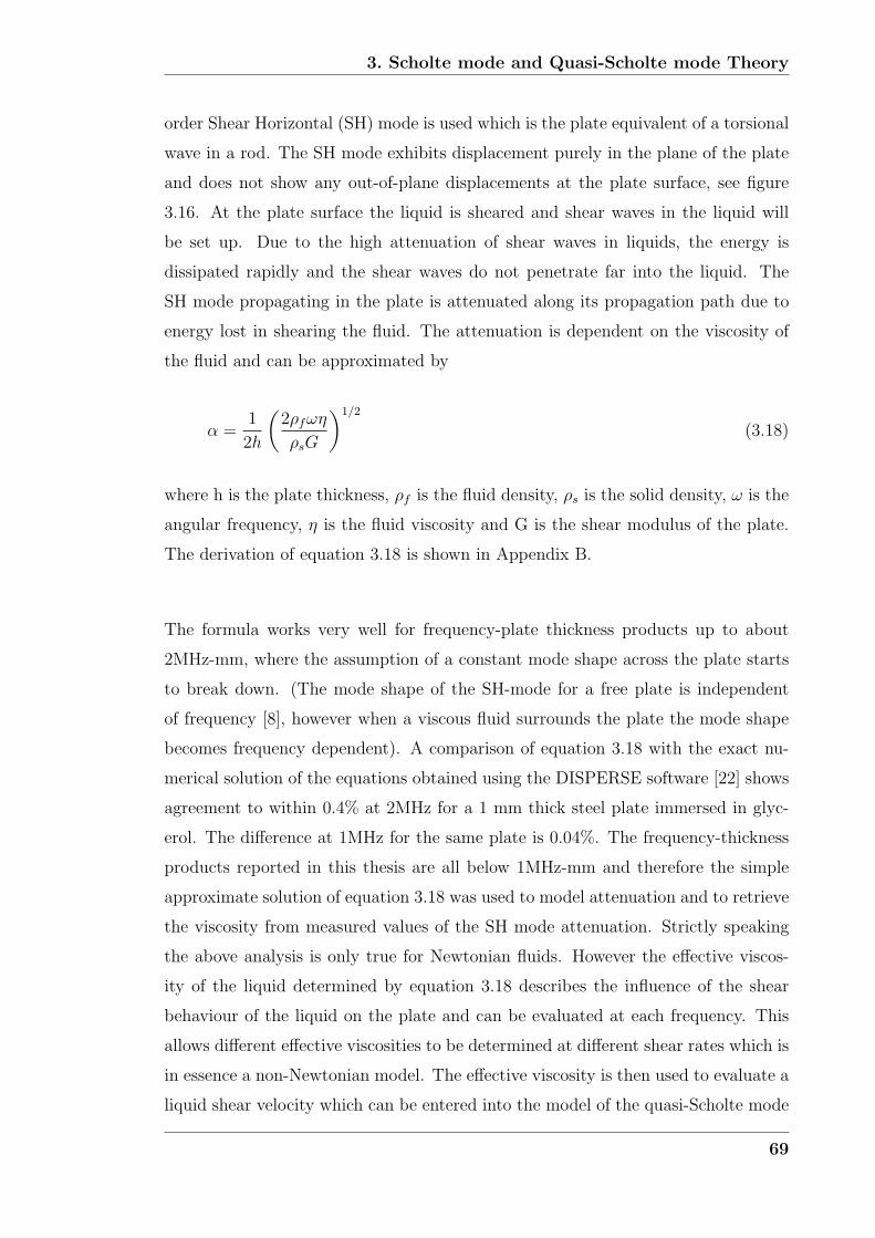
3. Scholte mode and Quasi-Scholte mode Theory
order Shear Horizontal (SH) mode is used which is the plate equivalent of a torsional
wave in a rod. The SH mode exhibits displacement purely in the plane of the plate
and does not show any out-of-plane displacements at the plate surface, see figure
3.16. At the plate surface the liquid is sheared and shear waves in the liquid will
be set up. Due to the high attenuation of shear waves in liquids, the energy is
dissipated rapidly and the shear waves do not penetrate far into the liquid. The
SH mode propagating in the plate is attenuated along its propagation path due to
energy lost in shearing the fluid. The attenuation is dependent on the viscosity of
the fluid and can be approximated by
α =1
2h
(2ρfωη
ρsG
)1/2
(3.18)
where h is the plate thickness, ρf is the fluid density, ρs is the solid density, ω is the
angular frequency, η is the fluid viscosity and G is the shear modulus of the plate.
The derivation of equation 3.18 is shown in Appendix B.
The formula works very well for frequency-plate thickness products up to about
2MHz-mm, where the assumption of a constant mode shape across the plate starts
to break down. (The mode shape of the SH-mode for a free plate is independent
of frequency [8], however when a viscous fluid surrounds the plate the mode shape
becomes frequency dependent). A comparison of equation 3.18 with the exact nu-
merical solution of the equations obtained using the DISPERSE software [22] shows
agreement to within 0.4% at 2MHz for a 1 mm thick steel plate immersed in glyc-
erol. The difference at 1MHz for the same plate is 0.04%. The frequency-thickness
products reported in this thesis are all below 1MHz-mm and therefore the simple
approximate solution of equation 3.18 was used to model attenuation and to retrieve
the viscosity from measured values of the SH mode attenuation. Strictly speaking
the above analysis is only true for Newtonian fluids. However the effective viscos-
ity of the liquid determined by equation 3.18 describes the influence of the shear
behaviour of the liquid on the plate and can be evaluated at each frequency. This
allows different effective viscosities to be determined at different shear rates which is
in essence a non-Newtonian model. The effective viscosity is then used to evaluate a
liquid shear velocity which can be entered into the model of the quasi-Scholte mode
69

3. Scholte mode and Quasi-Scholte mode Theory
([53], appendix A).
3.6 Summary
In this chapter the Scholte wave was introduced. Modelling techniques are well es-
tablished in the literature and have been summarised for ideal and viscous fluids in
contact with an elastic solid half space. Numerical results for Scholte wave phase
velocities and energy distribution between the two materials were presented for a
range of material property combinations. Then the quasi-Scholte mode plate mode
was introduced. The change of geometry from a half space to a plate immersed in
a fluid complicates the analysis slightly and mainly introduces a frequency depen-
dence of the quasi-Scholte mode characteristics. At high frequencies the plate mode
behaves like the Scholte wave on a half space. A physical explanation for this is that
the wavelength of the wave becomes very small compared to the plate thickness and
due to the evanescent nature of the Scholte wave only one interface is seen by the
wave. Two different attenuation mechanisms of the Scholte and quasi-Scholte wave
were identified: shear leakage and attenuation due to fluid bulk attenuation.
The sensitivity of the quasi-Scholte mode to several fluid bulk parameters has been
analysed. It was found that the group velocity of the quasi-Scholte mode is very
sensitive to the fluid bulk velocity. In the range of 0.25 − 0.5 MHz mm the group
velocity of the quasi-Scholte mode on a steel plate is most sensitive to the fluid bulk
velocity. The phase velocity is not as sensitive as the group velocity and since it
is more difficult to evaluate the phase velocity using a pulse echo measurement its
use is not recommended. The analysis revealed that the sensitivity to fluid shear
viscosity increases with increasing frequency. However it has to be kept in mind
that at higher frequencies the overall attenuation will be higher and can introduce
practical difficulties and sources of error. It was also found that the sensitivity to
bulk longitudinal attenuation increases from zero to unity in an ”S” shaped curve
with frequency. The transition region lies in the frequency thickness product range
of 0.25 − 0.5 MHz mm which corresponds to the range of maximum sensitivity of
the group velocity to the fluid bulk velocity. It is believed that this increase in
sensitivity is due to the fact that a higher fraction of the quasi-Scholte mode energy
70

3. Scholte mode and Quasi-Scholte mode Theory
is travelling in the fluid and thus the effect of the fluid properties is more strongly
reflected in the quasi-Scholte mode properties.
71

3. Scholte mode and Quasi-Scholte mode Theory
3.7 Figures
Figure 3.1: Sketch of the system used to study the Scholte wave
72
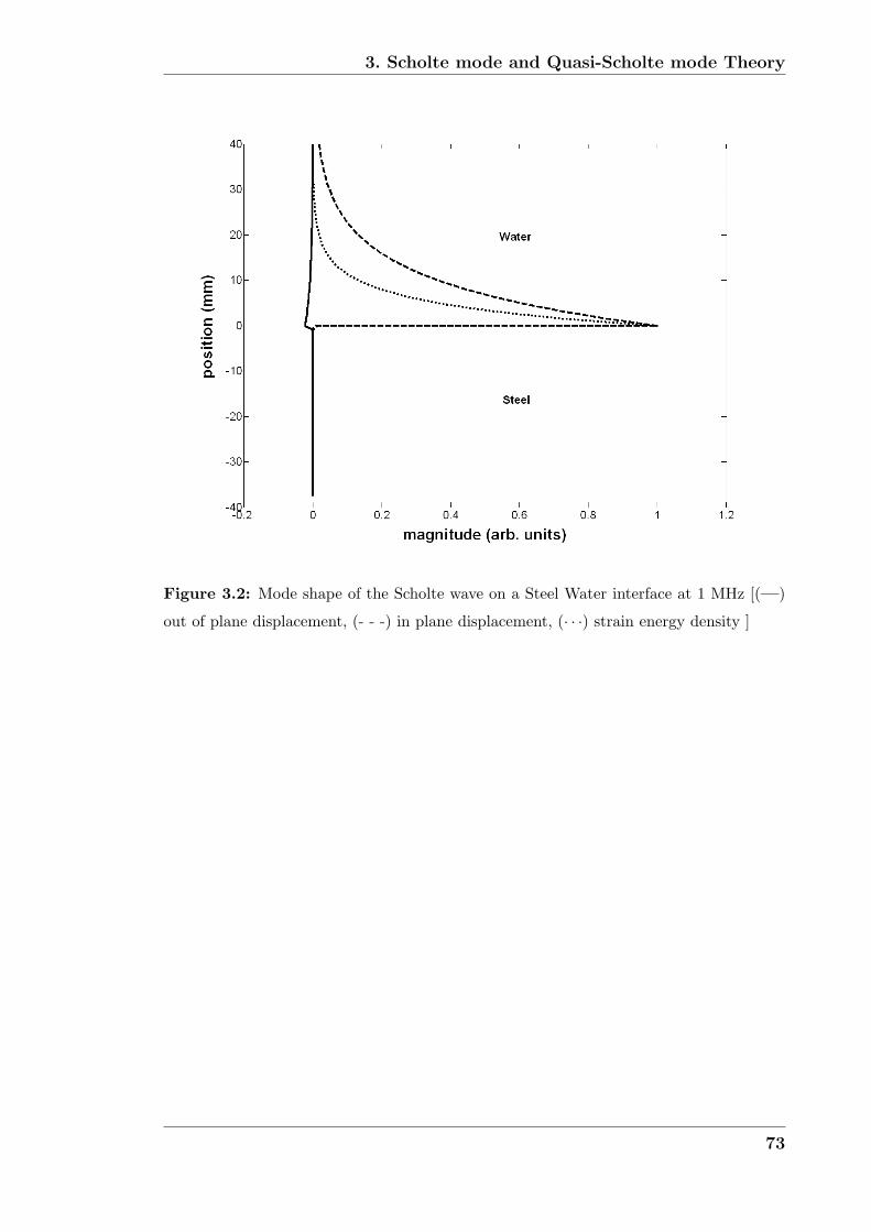
3. Scholte mode and Quasi-Scholte mode Theory
Figure 3.2: Mode shape of the Scholte wave on a Steel Water interface at 1 MHz [(—)
out of plane displacement, (- - -) in plane displacement, (· · ·) strain energy density ]
73
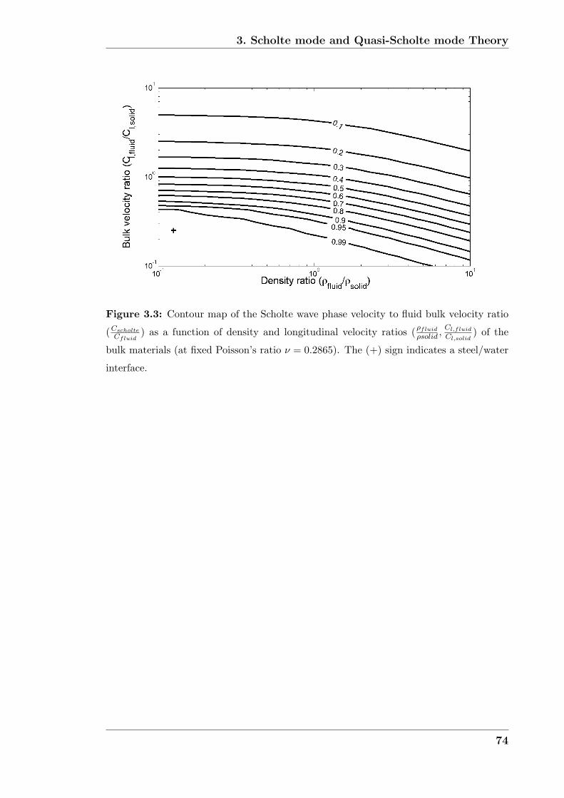
3. Scholte mode and Quasi-Scholte mode Theory
Figure 3.3: Contour map of the Scholte wave phase velocity to fluid bulk velocity ratio
(CscholteCfluid
) as a function of density and longitudinal velocity ratios (ρfluid
ρsolid ,Cl,fluid
Cl,solid) of the
bulk materials (at fixed Poisson’s ratio ν = 0.2865). The (+) sign indicates a steel/water
interface.
74

3. Scholte mode and Quasi-Scholte mode Theory
Figure 3.4: Contour map showing the fraction of Scholte wave energy that travels in the
fluid (Efluid
Etotal) as a function of density and longitudinal velocity ratios (ρfluid
ρsolid ,Cl,fluid
Cl,solid) of the
bulk materials. (at fixed Poisson’s ratio ν = 0.2865). The (+) sign indicates a steel/water
interface.
75

3. Scholte mode and Quasi-Scholte mode Theory
Figure 3.5: The phase velocity dispersion of the quasi-Scholte mode on a steel plate
surrounded by water (see text for material properties).
76
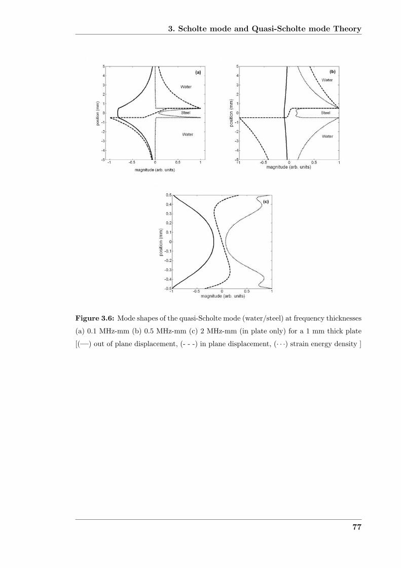
3. Scholte mode and Quasi-Scholte mode Theory
Figure 3.6: Mode shapes of the quasi-Scholte mode (water/steel) at frequency thicknesses
(a) 0.1 MHz-mm (b) 0.5 MHz-mm (c) 2 MHz-mm (in plate only) for a 1 mm thick plate
[(—) out of plane displacement, (- - -) in plane displacement, (· · ·) strain energy density ]
77
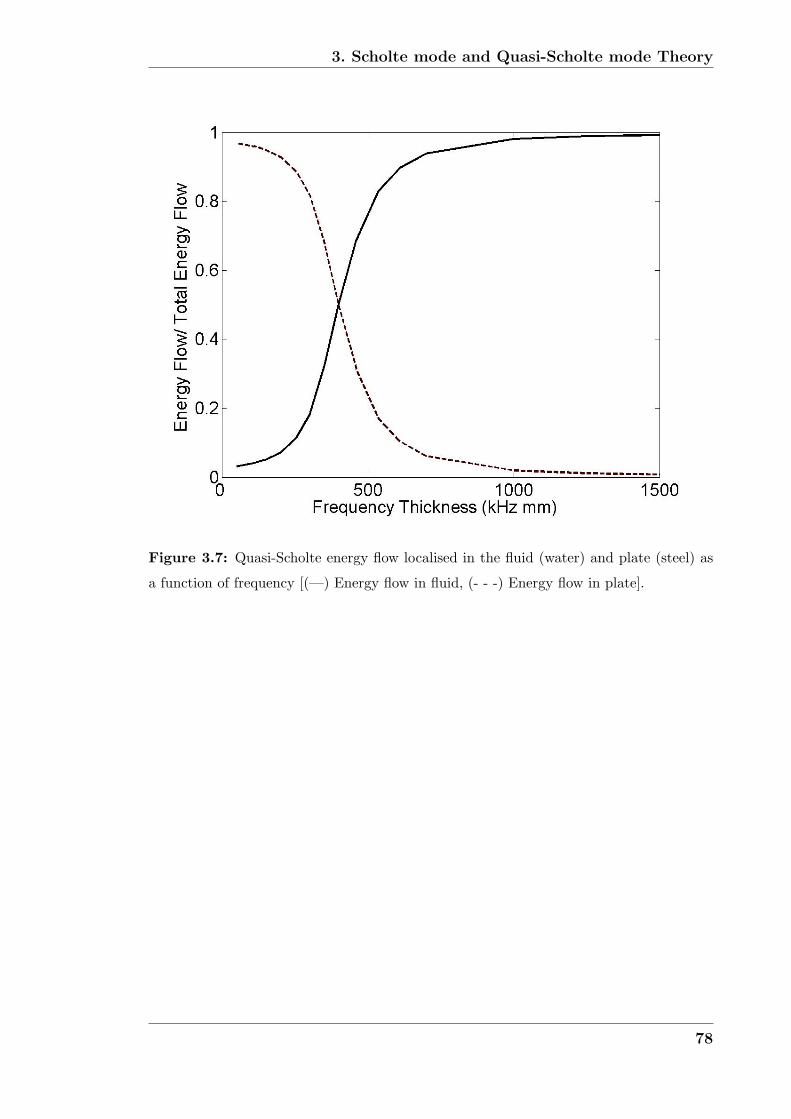
3. Scholte mode and Quasi-Scholte mode Theory
Figure 3.7: Quasi-Scholte energy flow localised in the fluid (water) and plate (steel) as
a function of frequency [(—) Energy flow in fluid, (- - -) Energy flow in plate].
78

3. Scholte mode and Quasi-Scholte mode Theory
Figure 3.8: Quasi-Scholte mode group velocities as a function of frequency for different
longitudinal bulk velocities (cl) (The other properties are as in figure 3.10)
79

3. Scholte mode and Quasi-Scholte mode Theory
Figure 3.9: Quasi-Scholte mode attenuation as a function of frequency for different
viscosities (η) at cl = 1800m/s (The other properties are as in figure 3.10)
80
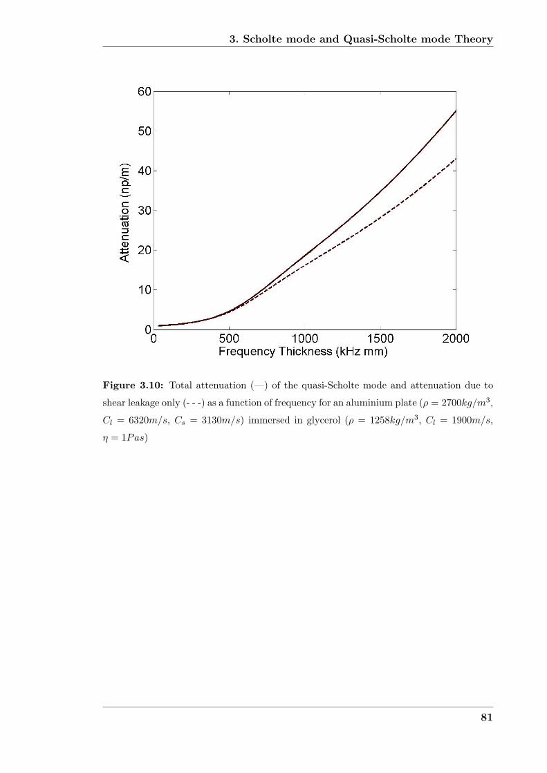
3. Scholte mode and Quasi-Scholte mode Theory
Figure 3.10: Total attenuation (—) of the quasi-Scholte mode and attenuation due to
shear leakage only (- - -) as a function of frequency for an aluminium plate (ρ = 2700kg/m3,
Cl = 6320m/s, Cs = 3130m/s) immersed in glycerol (ρ = 1258kg/m3, Cl = 1900m/s,
η = 1Pas)
81

3. Scholte mode and Quasi-Scholte mode Theory
Figure 3.11: Attenuation dispersion curves of the quasi-Scholte mode for a 0.105 mm
thick steel plate immersed in water of density 1000 kg/m3, bulk velocity 1500 m/s and
viscosity 1 mPas only (· · ·), viscosity 1 mPas and longitudinal attenuation 0.001 Np/wl (-
- -) and viscosity 1 mPas and longitudinal attenuation 0.002 Np/wl (—). The attenuation
unit Np/wl stands for Nepers per wavelength. The quasi-Scholte mode is attenuated by
shear leakage due to viscosity and an additional attenuation due to fluid longitudinal bulk
attenuation.
82

3. Scholte mode and Quasi-Scholte mode Theory
Figure 3.12: The group velocity sensitivity of the quasi-Scholte mode to a change in
fluid bulk velocity for a 1mm steel plate surrounded by water (ρsteel = 7932kg/m3,Cl =
5959.5m/s, Cs = 3260m/s, ρwater = 1000kg/m3, Cl = 1500m/s ).
83
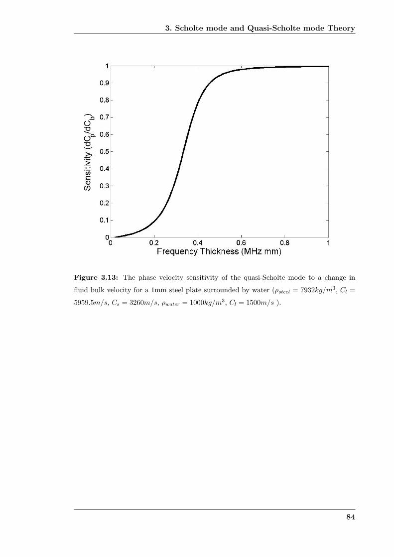
3. Scholte mode and Quasi-Scholte mode Theory
Figure 3.13: The phase velocity sensitivity of the quasi-Scholte mode to a change in
fluid bulk velocity for a 1mm steel plate surrounded by water (ρsteel = 7932kg/m3, Cl =
5959.5m/s, Cs = 3260m/s, ρwater = 1000kg/m3, Cl = 1500m/s ).
84
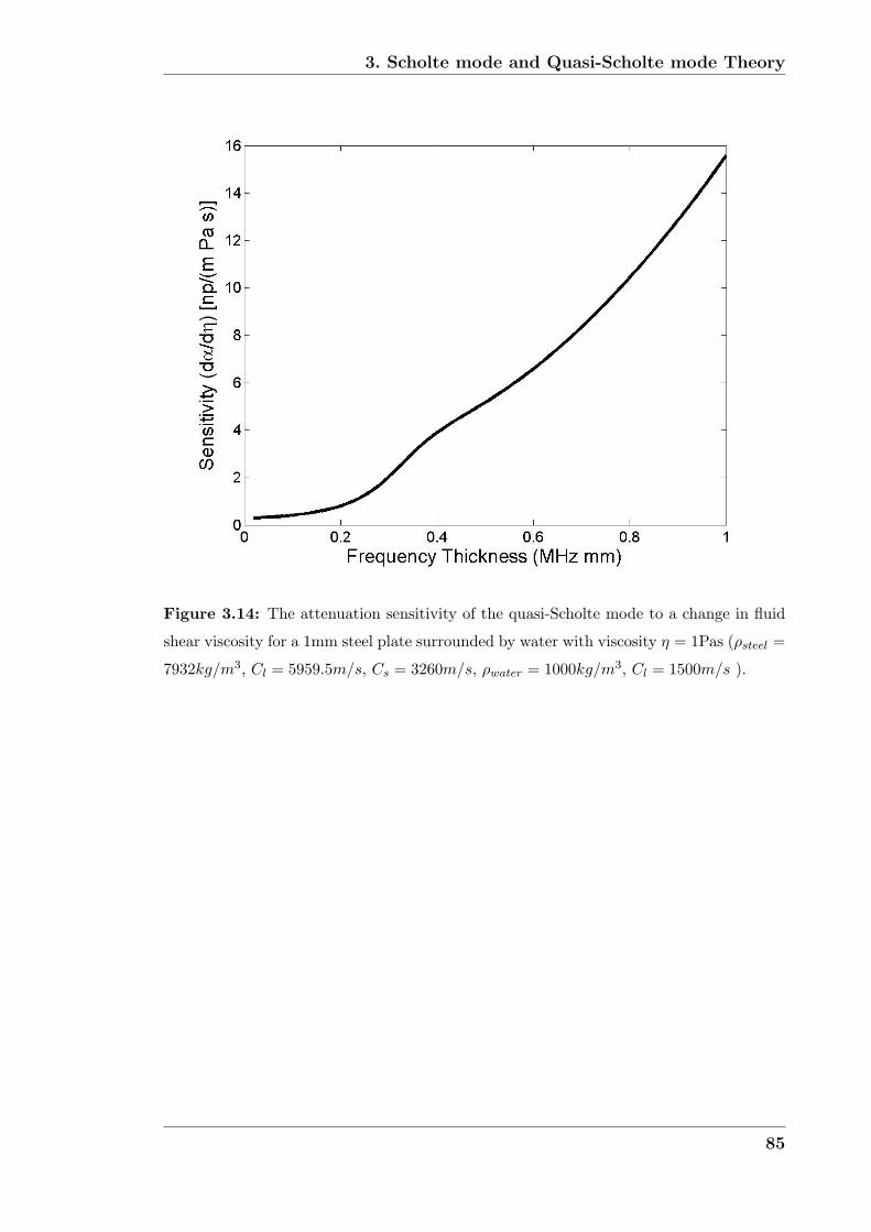
3. Scholte mode and Quasi-Scholte mode Theory
Figure 3.14: The attenuation sensitivity of the quasi-Scholte mode to a change in fluid
shear viscosity for a 1mm steel plate surrounded by water with viscosity η = 1Pas (ρsteel =
7932kg/m3, Cl = 5959.5m/s, Cs = 3260m/s, ρwater = 1000kg/m3, Cl = 1500m/s ).
85

3. Scholte mode and Quasi-Scholte mode Theory
Figure 3.15: The attenuation sensitivity of the quasi-Scholte mode to a change in fluid
longitudinal bulk attenuation for a 1mm steel plate surrounded by water with viscosity
ν = 1Pas and longitudinal bulk attenuation of α = 0.01 np/wl (ρsteel = 7932kg/m3,
Cl = 5959.5m/s, Cs = 3260m/s, ρwater = 1000kg/m3, Cl = 1500m/s ).
86
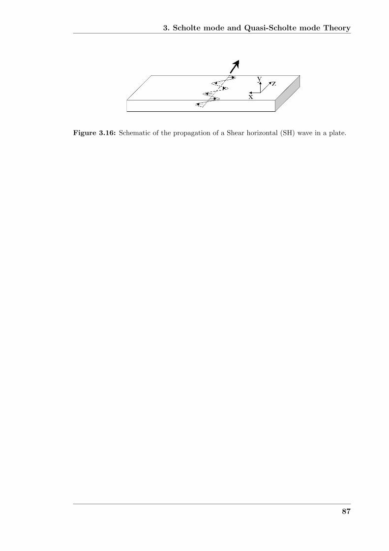
3. Scholte mode and Quasi-Scholte mode Theory
Figure 3.16: Schematic of the propagation of a Shear horizontal (SH) wave in a plate.
87
Chapter 4
Quasi-Scholte mode Experiments
4.1 Overview
A range of experiments was carried out to validate the results obtained by the
theoretical model described in chapter 3. Experimental results from QS mode mea-
surements were validated by measurements in a conventional ultrasonic test cell. In
section 4.2 methods of excitation of the Scholte and quasi-Scholte wave that have
been reported in the literature are discussed. One method of excitation was cho-
sen and a measurement apparatus was built. The basic apparatus that was used is
described in section 4.3. For the evaluation of fluid bulk attenuation an additional
measurement of the fluid shear properties is needed. The transduction method could
be altered to also excite a shear horizontal plate mode. The experimental arrange-
ment for this is described in section 4.4. Section 4.5 briefly presents the ultrasonic
test cell that was used for validation measurements. Then results are presented
in section 4.6. Some discrepancies between the test cell measurements and the QS
mode measurements were found. In section 4.7 possible error sources are considered.
These considerations will be useful for the design of a future QS mode measurement
apparatus. The experimental findings of this chapter are summarised in section 4.8.
88
4. Quasi-Scholte mode Experiments
4.2 Excitation of the Scholte and quasi-Scholte
mode
Many ways of exciting Scholte waves have been reported in the literature (see e.g.
[54],[55],[56],[57],[58]). Nasr et al. [54] and McLean et al. [55] used a comb-like
transducer (PVDF or micro-machined) that preferentially excites a certain wave-
length range at the interface of a solid and a liquid to excite Scholte waves. Desmet
et al. [56] used laser excitation to create the Scholte wave at the interface. DeBilly et
al. [57] and Matula et al. [58] used the concept of mode conversion from a Rayleigh
(or A0 wave on a plate) to the Scholte wave. They generated a clean mode on an
unimmersed section of the waveguide using conventional techniques, the wave then
propagates into the liquid and part of its energy converts into the Scholte mode.
This latter approach of mode conversion from an A0 plate wave was also chosen for
the experiments reported in this thesis. The method is reliable, cheap and easily set
up. It also separates the transducer from the embedding medium and thus does not
require the transducer to be submerged in the liquid. This prevents bulk waves that
travel parallel to the interface from being setup in the liquid at the same time as the
Scholte wave. It also separates the transducer from harsh environments like high
temperature, highly corrosive or radioactive fluids. Wedge like methods (excitation
by means of angled incidence) were ruled out because a fluid of lower bulk velocity
than the embedding fluid bulk velocity is needed. Attaching this wedge or angled
fluid channel to the waveguide would become difficult and changes of incident angle
as required for producing different wavenumbers would be technically challenging
and make the device cumbersome.
The method of mode conversion that was chosen to excite the quasi-Scholte mode
in a plate fluid system also has shortcomings. Mode conversion is not efficiently
achieved at all frequencies. Notably, at high frequencies the efficiency of mode con-
version from the A0 mode of a free plate to the quasi-Scholte mode of an immersed
plate is low. An explanation for this can be found in the distribution of mode en-
ergy within the QS mode as shown in figure 3.7. At high frequencies, above 500
kHz-mm, almost all of the QS mode energy travels in the fluid, which means that
89

4. Quasi-Scholte mode Experiments
excitation from the plate will be difficult. However the energy of the incident A0
mode is entirely located in the plate. The mode shapes of the A0 mode of the free
plate and the QS mode, while very similar at low frequencies, become more and
more different at high frequencies. This trend is also illustrated in the wavenumber
dispersion curves of the free plate A0 mode and the QS mode. Figure 4.1 shows
that at low frequency thicknesses (< 500 kHz-mm) the wavenumbers of the A0 mode
of a free plate and the QS mode of an immersed plate are similar while at higher
frequency thicknesses they tend apart. The wavenumber of the leaky A0 mode of an
immersed plate is also displayed. Tracing of this mode is very difficult and its be-
haviour is anomalous at low frequency thicknesses (see Dickey et al. [59]) therefore
the mode has only been displayed from frequency thicknesses above 220 kHz-mm
where it becomes supersonic with respect to the embedding fluid bulk velocity. For
the purposes here this is sufficient to illustrate that the wavenumber of the leaky
A0 mode tends away from the free plate A0 mode wavenumber at low frequency
thicknesses. The mode shapes of all three modes in the plate are very similar at
frequency thickness products below 0.6 MHz-mm. Mode conversion from the free
plate A0 mode favours the QS mode at low frequency thicknesses and the leaky A0
mode at higher frequency thickness products.
Since the quasi-Scholte mode is more sensitive to fluid properties at higher frequen-
cies there is an optimum frequency window in which the method of mode conversion
from the A0 to QS mode works and at the same time information can be extracted
from the fluid. It is important to excite the QS mode strongly in a frequency thick-
ness window where it is sensitive to the fluid but also still excitable. This window
was found to lie between 200 and 400 kHz-mm for a steel plate immersed in wa-
ter. The window will shift slightly for different plate materials and liquids that are
interrogated but no drastic changes are expected.
4.3 The setup
The experimental setup used was designed to excite the quasi-Scholte mode on
a plate immersed in a fluid and to measure its group velocity and attenuation.
Figure 4.2 shows a schematic of the apparatus. A shear transducer was attached
90
4. Quasi-Scholte mode Experiments
to the centre of an end of a plate. It was attached in such a way that it would
produce out-of-plane movements uniformly across the thickness of the plate. This
was known to excite the A0 mode of a free plate reliably. Figure 4.3 shows the
configuration of transducer and plate. Plates of two different thicknesses were used
to excite the quasi-Scholte mode within two different frequency thickness ranges.
The first plate was made out of Aluminium (ρ = 2700kg/m3, Cl = 6320m/s and
Cs = 3130m/s) and had a thickness of 0.94 mm, the second plate was made of
stainless steel (ρ = 7764kg/m3, Cl = 6000m/s and Cs = 2700m/s) and was 0.105
mm thick. The material properties were determined by velocity measurements of
the fundamental guided wave modes. The Aluminium plate was 100 mm wide and
200 mm long, while the stainless steel plate was 96 mm wide and 135 mm long.
A 500 kHz shear transducer (Panametrics Inc.) was used to excite the A0 mode in
the Aluminium plate while a 5 MHz shear transducer (Panametrics Inc.) was used
for the thinner stainless steel plate. Transducers were either coupled to the plate by
clamping them onto the cross section using treacle as shear couplant or by bonding
them with epoxy.
A vessel containing a fluid sample was placed beneath the plate on a table of variable
height. By changing the height of the table the plate could conveniently be immersed
in the fluid to different depths; the angle between the fluid surface and the plate
was 90 degrees.
The fluid temperature was recorded using a thermocouple that was immersed in
the liquid. The whole setup could also be placed in a temperature controlled en-
vironment as was done for measurements on suspensions. The signal was sent and
received by a waveform generator (Macro Design Ltd.), a LeCroy 9400A Storage Os-
cilloscope was used to store the signal and the data was then transferred to a PC for
processing. The transducer was excited with a Hanning windowed toneburst. The
excited A0 wave travelled along the plate until it hit the fluid surface. Here part of
the wave was reflected back as an entry reflection and the rest converted into modes
in the fluid-plate system: a highly attenuated leaky A0 mode and the quasi-Scholte
mode. After a short propagation distance only the quasi-Scholte mode remained.
It was reflected by the end of the plate and converted back into an A0 mode at the
point where the plate leaves the liquid (some energy was also reflected back into
91

4. Quasi-Scholte mode Experiments
the fluid). The wave then propagated along the plate structure until it reached the
transducer again. A typical time trace is displayed in figure 4.4. The entry reflec-
tion, plate end reflection and a reverberation in the fluid are clearly visible. Data
for tonebursts at different centre frequencies and two different immersion depths
were collected for the aluminum plate setup. For later experiments on the thinner
stainless steel plate the technique was further developed and only one broadband
signal was sent and received.
The group velocity and attenuation of the quasi-Scholte mode were then extracted
from the collected data using the following equations:
Cg =2(x2 − x1)(
ΔT + 2(x2−x1)CgA0
) (4.1)
α = − 1
2(x2 − x1)ln
(S2(ω)
S1(ω)
)(4.2)
where x1 < x2 are two different immersion depths, ΔT is the time difference between
the arrival of the wave packages at the two immersion states, CgA0 is the group ve-
locity of the A0 free plate mode and S1 and S2 are the signal amplitudes at the
respective immersion depths.
In order to eliminate the effects of dispersion on the measured attenuation the mag-
nitude of the Fourier transform at the centre frequency of each toneburst was used
in equation 4.2. For the aluminium plate the difference in arrival time ΔT was eval-
uated by cross correlating the signals at the two immersion depths. The maximum
of this function corresponds to the time shift between the two signals [58]. The cross
correlation method could be used in this case because signals of a narrow bandwidth
were used and propagation distances were short so that dispersion effects were neg-
ligible. In the setup of the stainless steel plate two other methods of evaluating
the time shift between signal arrivals were used: the amplitude spectrum method
(see Pialucha et al. [60]) and the method of zero phase slope, which is described in
Appendix C.
92
4. Quasi-Scholte mode Experiments
The wavenumber in both systems (plate only, plate-fluid) is very similar so it is
assumed that beam spreading effectively stays constant. It was verified that the
plate was large enough and that reflections from the plate edges were not present in
the recorded signal by a simple experiment: pressure was applied to the surfaces of
the plate by squeezing it between the fingers. This has the effect of damping the wave
propagating across the point where pressure is applied. When the plate was squeezed
at the centre the signal was almost completely attenuated while pressing the sides,
edges and corners did not have any identifiable effect on the signal amplitude.
4.4 SH wave attenuation measurements
At the end of section 3.3 the need for a determination of liquid shear properties in
order to measure bulk longitudinal attenuation using the quasi-Scholte mode was
expressed. It was found that the setup of the plate and transducer could easily be
adjusted to excite SH waves simultaneously to the QS mode. This is possible due
to the different velocities of the modes and the temporal separation that this causes
between the signals. Figure 4.5 shows two time traces obtained using the stainless
steel plate setup, in which the transducer polarisation and the plate were slightly
misaligned. Arrivals of 3 signal packets can clearly be differentiated. They corre-
spond to the three different lowest order propagating modes of the plate: S0, SH0
and A0 converted into QS mode in the immersed section. The excitation of the S0
and SH0 mode is caused by misalignment of the transducer polarisation direction
with the plane of the plate. The arrival of the SH wave is indicated in figure 4.5
where the plate and transducer were slightly misaligned while it is not visible in
figure 4.4 where better alignment between transducer polarisation direction and the
plane of the plate were achieved. The attenuation of the signal is easily analysed as
for the QS mode signal, see equation 4.2.
Equation 3.18 can be used to retrieve the viscosity of the liquid from the SH wave
attenuation measurement. As mentioned in section 3.5 the analysis is strictly only
true for Newtonian liquids. If however an effective viscosity is determined at each
frequency, the shear behaviour of the liquid is adequately retrieved and accounted
93
4. Quasi-Scholte mode Experiments
for.
4.5 Ultrasonic Test cell
An alternative method of determining the fluid bulk properties was needed to vali-
date the results from the quasi-Scholte mode measurements. An ultrasonic test cell
that was developed at the University of Nottingham (UK) [61] was used to carry out
these validation measurements of fluid bulk velocity and attenuation. This setup
consisted of a transducer at one end of the cell which sent a wide bandwidth signal
across the fluid sample to a receiver. The exciter and receiver were thick slabs of
piezo-electric material. The time delay and amplitude loss were then used to obtain
the velocity and attenuation in the sample. This technique is standard and the
reader is referred to Challis et al. [61] for further details. Sample sizes were about
25 ml for the test cell and the fluid could be temperature controlled to within 0.1
degrees centigrade. Figure 4.6 shows a schematic of the test cell.
4.6 Results
4.6.1 Newtonian Fluids
The quasi-Scholte mode measurement method was first tried on Newtonian fluids.
The parameters to be determined were the bulk velocity and viscosity of the fluid.
Glycerol was chosen as the test fluid. The density of a glycerol sample was measured
to be 1258kg/m3 and the aluminium plate properties were evaluated experimentally
as ρ = 2700kg/m3, Cl = 6320m/s and Cs = 3130m/s. The temperature was de-
termined to be 23◦C. Results were extracted from the time traces as described in
section 4.3. Figure 4.7(a) shows the measured group velocity of the quasi-Scholte
mode as a function of frequency and a theoretically modelled curve (DISPERSE
[22]) was fitted to the measured data. For the low viscosities of glycerol, the group
velocity dispersion relation of the quasi-Scholte mode is essentially only dependent
on the longitudinal velocity as described in section 3.3. Thus it is possible to extract
94
4. Quasi-Scholte mode Experiments
the longitudinal bulk velocity of the glycerol as 1930 m/s. Figure 4.7(b) shows the
measured and theoretically predicted attenuation for the quasi-scholte mode. The
measured attenuation fits best to a predicted viscosity of 0.82 Pas. An estimate of
the error in the measured viscosity, based on repeatability, is about 8%.
To validate the above results a measurement of the bulk longitudinal velocity was
carried out. This yielded a value of 1900 m/s. Also an alternative method of mea-
suring viscosity was utilised; this method involved the measurement of the torsional
T(0) mode attenuation of a rod immersed in glycerol as described by [36]. Using this
approach the viscosity was determined to be 0.89 Pas. The measurement environ-
ment for this experiment, unlike later experiments, was not temperature controlled.
The humidity was not controlled either but the two experiments were carried out
almost simultaneously (less than 10 minutes apart). The measured results compared
well to each other and literature data. Kaye and Laby [62] state the viscosity of
99% glycerol to be 0.9 Pas at 23◦C.
The quasi-Scholte mode was also used to measure the properties of honey. Figure
4.8(a) shows the measured group velocity and figure 4.8(b) shows the measured at-
tenuation of the quasi-Scholte mode of the 0.94mm aluminium plate immersed in
honey (Gale’s Clear Honey, Premier Ambient Products (UK) Ltd., Spalding PE12
9EQ). The average bulk velocity of the honey was determined to be 2140 ± 30 m/s
and the average viscosity was evaluated at 19.2 ± 1.17 Pas, where the quoted un-
certainty is based on repeatability of the measurement results.
The results for honey show that the method also works for very viscous fluids. De-
spite its many different constituents the behaviour of honey is described well by
a Newtonian fluid [63]. As stated in section 3.2.2 low viscosities (< 30 Pas) are
currently assumed in the modelling of the quasi-Scholte mode and therefore errors
will introduce if the same model is used for highly viscous liquids. Honey is still
modelled well by assuming low viscosities, however high viscosity formulations for
equations 3.7-3.10 can be implemented [22] for more viscous fluids. High viscosity
fluids will also exhibit significant shear leakage that can partially be limited by al-
95
4. Quasi-Scholte mode Experiments
tering measurement frequency and propagation length. Highly viscous liquids will
also affect the quasi-Scholte mode group velocity which complicates the extraction
of bulk velocity and attenuation.
To facilitate the extraction of fluid bulk properties from the measured quasi-Scholte
mode data an inversion technique was developed. An iterative routine was pro-
grammed that automatically traced the quasi-Scholte mode group velocity disper-
sion curves for a given embedding fluid bulk velocity and viscosity. The result was
compared to the measured data points and the fluid bulk velocity was adjusted in the
right direction to reduce the mismatch between prediction and measurement. Once
a prediction point below and above the measured data was obtained a bi-section
scheme reduced the step size of the iteration. A maximum limit of iterations was
set and a result within a tolerance of 0.1 m/s or Np/m was accepted as a successful
iteration.
The iteration and inversion technique was first tested on a sample of distilled water
and a 5% ethanol-distilled water solution. To increase the range of bulk velocities
that could be measured the sample solutions were measured at different tempera-
tures between 10 and 30 degrees centigrade. The stainless steel plate was used to
carry out the measurements. Results are displayed in figure 4.9. The marker of the
bulk velocity indicates the mean velocity obtained from the inversion routine, while
the error bars indicate the standard deviation of the set of values obtained at differ-
ent frequencies from the mean value. Distilled water and the ethanol-water mixture
are non-dispersive fluids so that the velocity should be the same at all frequencies.
However due to noise in the group velocity measurement, and errors, slight differ-
ences in velocity at different frequencies are obtained. The mean value is also offset
from the theoretically predicted curve. This is believed to be due to the positioning
uncertainty of the plate (0.5%). Even with these errors in the data the measure-
ment results compare very well to literature data that was obtained from Povey [1].
The trend of increased velocity at increased temperature is clearly reflected by the
measurements in figure 4.9.
96
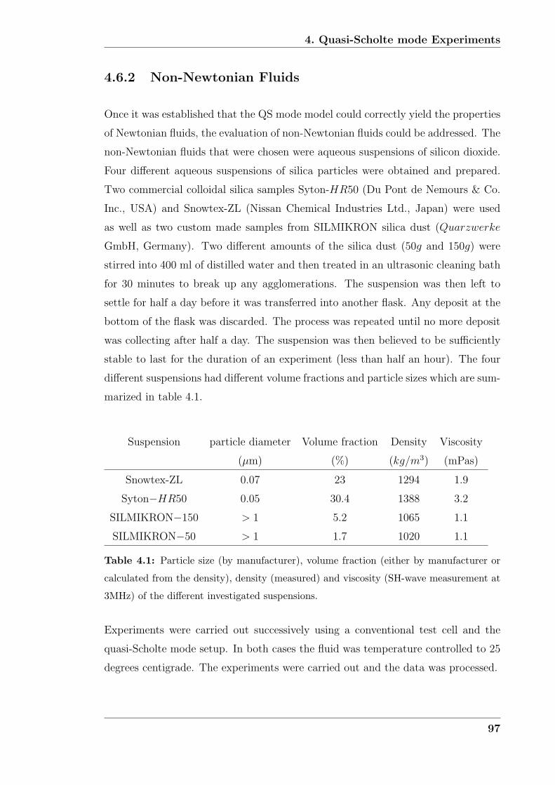
4. Quasi-Scholte mode Experiments
4.6.2 Non-Newtonian Fluids
Once it was established that the QS mode model could correctly yield the properties
of Newtonian fluids, the evaluation of non-Newtonian fluids could be addressed. The
non-Newtonian fluids that were chosen were aqueous suspensions of silicon dioxide.
Four different aqueous suspensions of silica particles were obtained and prepared.
Two commercial colloidal silica samples Syton-HR50 (Du Pont de Nemours & Co.
Inc., USA) and Snowtex-ZL (Nissan Chemical Industries Ltd., Japan) were used
as well as two custom made samples from SILMIKRON silica dust (Quarzwerke
GmbH, Germany). Two different amounts of the silica dust (50g and 150g) were
stirred into 400 ml of distilled water and then treated in an ultrasonic cleaning bath
for 30 minutes to break up any agglomerations. The suspension was then left to
settle for half a day before it was transferred into another flask. Any deposit at the
bottom of the flask was discarded. The process was repeated until no more deposit
was collecting after half a day. The suspension was then believed to be sufficiently
stable to last for the duration of an experiment (less than half an hour). The four
different suspensions had different volume fractions and particle sizes which are sum-
marized in table 4.1.
Suspension particle diameter Volume fraction Density Viscosity
(μm) (%) (kg/m3) (mPas)
Snowtex-ZL 0.07 23 1294 1.9
Syton−HR50 0.05 30.4 1388 3.2
SILMIKRON−150 > 1 5.2 1065 1.1
SILMIKRON−50 > 1 1.7 1020 1.1
Table 4.1: Particle size (by manufacturer), volume fraction (either by manufacturer or
calculated from the density), density (measured) and viscosity (SH-wave measurement at
3MHz) of the different investigated suspensions.
Experiments were carried out successively using a conventional test cell and the
quasi-Scholte mode setup. In both cases the fluid was temperature controlled to 25
degrees centigrade. The experiments were carried out and the data was processed.
97
4. Quasi-Scholte mode Experiments
The measured quantities from the quasi-Scholte mode and ultrasonic test cell ex-
periments do not yield comparable quantities, they have to be converted and can
then be compared in two different ways: the forward model and the inverted model.
The forward problem consists of determining the dispersion curves for the quasi-
Scholte mode from the measured bulk wave velocity and attenuation in the ultra-
sonic test cell. Group velocity as well as the attenuation of the quasi-Scholte mode
are determined as functions of frequency for a given set of input parameters which
are either known or determined from the ultrasonic test cell measurement. There
are fixed input parameters (plate material density, plate material longitudinal and
transverse bulk velocity) and variable input parameters (fluid density, fluid longitu-
dinal and shear wave velocity, fluid longitudinal and shear wave attenuation). Now
the dispersion curves obtained by modelling the plate surrounded by a fluid whose
properties were determined by the ultrasonic test cell could be compared to the
actually measured dispersion curves in the quasi-Scholte mode experiment.
In the inversion the measured properties (group velocity and attenuation) of the
quasi-Scholte mode are inverted to obtain the properties of the fluid that an ultra-
sonic test cell would deliver (bulk wave velocity and bulk wave attenuation). The
approach developed here used an iteration to evaluate the fluid bulk properties. An
initial guess for the fluid properties is used to evaluate the quasi-Scholte mode prop-
erties in the forward model. The measured data and the predicted data are compared
and the fluid properties are adjusted before they are re-entered into the global ma-
trix (see appendix A). Two parameters are adjusted simultaneously: longitudinal
bulk velocity and the part of the longitudinal attenuation which is in excess of the
viscosity induced dissipation. The parameters are increased in constant steps. A
bi-section scheme is used once two consecutively entered fluid property values yield
a result either side of the measured quasi-Scholte data point. The procedure is re-
peated until the modelled solution agrees to within a tolerance value (0.1 m/s, 0.1
Np/m) with the measured quasi-Scholte mode data.
98

4. Quasi-Scholte mode Experiments
The forward model
Figure 4.10 displays the measured group velocity of the quasi-Scholte mode and the
predicted group velocity obtained by modelling the fluid properties measured in the
ultrasonic test cell. The results in figure 4.10 show a very good agreement of the
predicted and measured values. The lines trace the same path and only small devi-
ations from the predicted values are seen in the actual measurement. The errors in
the measured velocity are surprisingly small; a positioning accuracy of 0.5% in the
immersion depth of the plate explains the different offsets for the curves of the four
samples.
Figure 4.11 displays the measured attenuation of the quasi-Scholte mode and the
predicted attenuation obtained by forward modelling using the fluid properties mea-
sured in the ultrasonic test cell. The results show good agreement between mea-
surements of the quasi-Scholte mode attenuation and the predicted quasi-Scholte
mode attenuation obtained from the fluid property measurement (bulk velocity CL
and bulk attenuation α) in a test cell for the commercially obtained colloidal silica
samples. The attenuation of the purpose made SILMIKRON samples still agreed
well in trend but were offset by about 20% above the prediction from the bulk
wave measurement. The attenuation measurement is more prone to the influence
of errors, see section 4.7. In order to reduce the effects of noise in the measured
attenuation data a quadratic curve was fitted to it. The error bars in figure 4.11
indicate the standard error (< 0.5%) of the attenuation data and the curve fit. (The
error bars in the attenuation graph of figure 4.11 appear smaller than the error bars
of the velocity graph of figure 4.10. However this is simply due to the expanded
scale of figure 4.10, the percentage velocity error is substantially smaller than the
percentage attenuation error.)
The higher values of attenuation of the SILMIKRON suspension indicate the sen-
sitivity of the quasi-Scholte mode to non-viscous dissipative mechanisms in fluids.
The viscosities of the commercial samples Snowtex-ZL and Syton-HR50 are greater
by a factor of 2 and 3 respectively (see Table 4.1), however the quasi-Scholte mode
measurement reveals a lower attenuation than for the SILMIKRON samples. The
99
4. Quasi-Scholte mode Experiments
loss of energy into the embedding liquid due to shear coupling in the SILMIKRON
samples must be less than that for the commercial samples. If viscosity was the
only attenuation mechanism, SILMIKRON should exhibit a lower attenuation than
the commercial samples, but the measured attenuation in the SILMIKRON samples
was higher. This is due to scattering of the wave at particles in the suspension; it
is well known that scattering increases attenuation in fluids [3].
However the total attenuation of the quasi-Scholte mode is not as high as the atten-
uation experienced by a bulk wave in the strongly scattering SIMLIKRON fluids.
This is because only a fraction ( 20-40% depending on the frequency) of the en-
ergy of the quasi-Scholte mode travels in the embedding fluid see chapter 3. This is
an attractive feature for the investigation of highly attenuative and scattering fluids.
Inversion
The inversion technique was then used on the silica suspension data. The results
from the velocity inversion are summarised in figure 4.12. The agreement between
the test cell measurements and the inverted quasi-Scholte mode measurements is
good. The errors that were apparent in the forward model (section 4.6.2) are re-
tained. The mean values of the lines are also offset by up to 0.5%, which is believed
to be caused by the uncertainty with which the immersion depth of the plate is
determined.
The results in figure 4.13 show the longitudinal bulk wave attenuation obtained
from the inversion of the quasi-Scholte measurements. These results show worse
agreement compared to the forward modelled data. Qualitatively the method cor-
rectly identifies the magnitude of the attenuation in the samples: SILMIKRON-150
exhibits the most attenuation, then SILMIKRON-50, while Snowtex-ZL and Syton-
HR50 are least attenuating. However the quantitative values differ from those ob-
tained using the ultrasonic test cell, sometimes by more than 25%. As in the forward
approach the inverted quasi-Scholte mode data shows a consistently higher attenu-
100
4. Quasi-Scholte mode Experiments
ation than the test cell measurements. Error bars in figure 4.13 show the standard
error introduced by using a quadratic curve fit to represent measured quasi-Scholte
mode data.
At low frequencies the error in attenuation is greatest; this is believed to be partly
due to the curve fit that seems to be less good at low frequencies but could also
be due to the fact that less energy travels in the liquid at low frequencies. The
sensitivity to the fluid properties is also not as high at low frequencies as it is at
high frequencies see section 3.4.
4.7 Error considerations
In order to allow future refinement of the QS mode measurement technique, sources
of error in the measurement had to be identified. The errors in the velocity mea-
surement, the attenuation measurement and processing of data were considered
separately.
The sources of error in the velocity measurements are the most obvious. The sam-
pling frequency of the digitizer which records the signal introduces the most basic
uncertainty in the velocity measurement by limiting the temporal resolution of the
signal acquisition. Noise in the received signal represents another source of error. If
processing is carried out in the time domain this can cause errors in the detection of
the arrival of a peak amplitude for example. However since the signal to noise ratio
and the sampling frequency were large in all measurements these errors were small.
The main uncertainty that entered the velocity measurement was believed to be the
uncertainty with which the immersion depth could be determined. The immersion
depth was determined visually by means of a ruler. This was believed to be accu-
rate to within 0.5 − 1.5% depending on the care taken and the overall distance to
be measured. Indeed the velocity measurements that were carried out agreed with
validation measurements and literature data within this range of uncertainty.
101
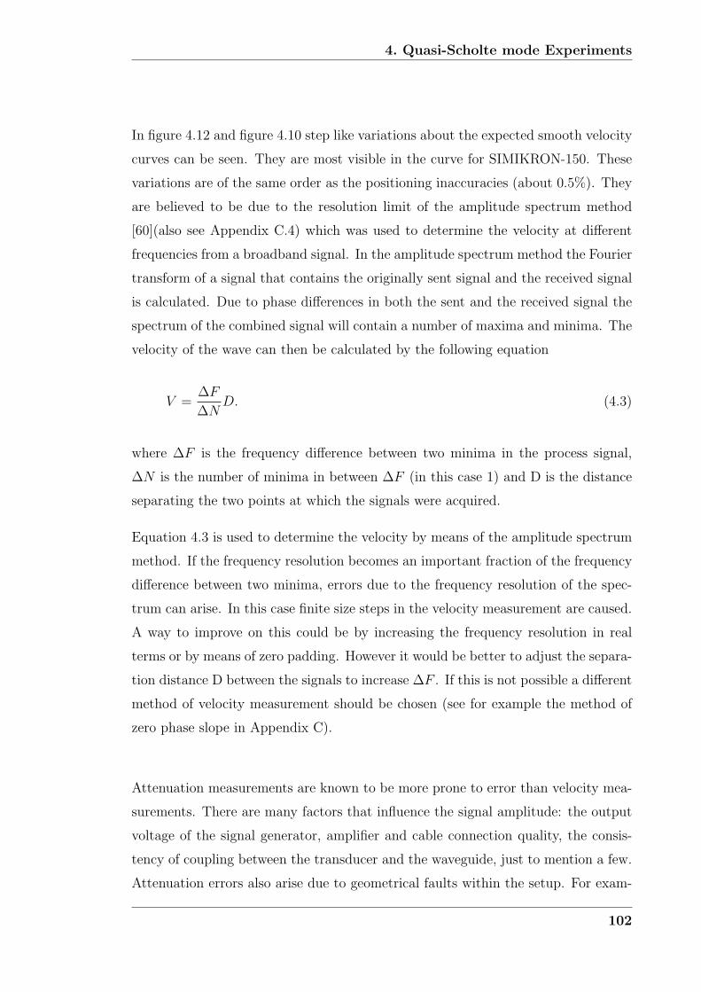
4. Quasi-Scholte mode Experiments
In figure 4.12 and figure 4.10 step like variations about the expected smooth velocity
curves can be seen. They are most visible in the curve for SIMIKRON-150. These
variations are of the same order as the positioning inaccuracies (about 0.5%). They
are believed to be due to the resolution limit of the amplitude spectrum method
[60](also see Appendix C.4) which was used to determine the velocity at different
frequencies from a broadband signal. In the amplitude spectrum method the Fourier
transform of a signal that contains the originally sent signal and the received signal
is calculated. Due to phase differences in both the sent and the received signal the
spectrum of the combined signal will contain a number of maxima and minima. The
velocity of the wave can then be calculated by the following equation
V =ΔF
ΔND. (4.3)
where ΔF is the frequency difference between two minima in the process signal,
ΔN is the number of minima in between ΔF (in this case 1) and D is the distance
separating the two points at which the signals were acquired.
Equation 4.3 is used to determine the velocity by means of the amplitude spectrum
method. If the frequency resolution becomes an important fraction of the frequency
difference between two minima, errors due to the frequency resolution of the spec-
trum can arise. In this case finite size steps in the velocity measurement are caused.
A way to improve on this could be by increasing the frequency resolution in real
terms or by means of zero padding. However it would be better to adjust the separa-
tion distance D between the signals to increase ΔF . If this is not possible a different
method of velocity measurement should be chosen (see for example the method of
zero phase slope in Appendix C).
Attenuation measurements are known to be more prone to error than velocity mea-
surements. There are many factors that influence the signal amplitude: the output
voltage of the signal generator, amplifier and cable connection quality, the consis-
tency of coupling between the transducer and the waveguide, just to mention a few.
Attenuation errors also arise due to geometrical faults within the setup. For exam-
102

4. Quasi-Scholte mode Experiments
ple refraction of the travelling wave at the position where the waveguide enters the
fluid can occur. The quasi-Scholte mode velocity is considerably slower than the A0
velocity of the free plate. If the wave enters the liquid at an angle different from
the normal, the beam will be refracted and on return to the transducer its position
will be offset slightly. A considerable decrease in amplitude can be observed at the
transducer; this effect was verified experimentally: a possible remedy is the change
from the plate geometry to a rectangular cross section strip.
The uncertainty with which the immersion depth is determined also introduces an
error in the attenuation measurement. On top of this, noise always enters the mea-
surement and in order to avoid larger errors due to the noise in the signal the overall
attenuation has to lie between 0.5 and 1 Np/m. This is an inherent problem with
any attenuation measurement which has been pointed out by Kalashnikov and Chal-
lis [42].
Finally errors can also enter the final result due to errors in processing techniques.
Several error sources within processing have been identified. When the group veloc-
ity and attenuation spectra of the measured signals were processed small oscillations
about a general curve trend were observed. To smoothen out these oscillations a
curve fit was used. The standard deviation of the curve fit from the actual data
was very small (< 0.5%). A quadratic curve was used as fit partly because the
viscous part of the attenuation is expected to vary with the square of frequency and
the velocity also has the shape of an inverted parabola.Figure 4.14 illustrates mea-
surement data and the respective curve fit. The use of this curve fit can cause errors.
During processing the accumulation of errors from the individual required measure-
ments also takes place. For example measurements of the plate material properties,
fluid density and viscosity are needed together with the QS-mode measurement to
process the final result. The A0 free plate mode group velocity is also required to
calculate the QS-mode velocity, see equation 4.1. An error in this A0 group velocity
measurement will directly enter the QS-mode group velocity result.
103
4. Quasi-Scholte mode Experiments
Another potential source of large error can be found in the processing of the lon-
gitudinal bulk attenuation from the measured QS-mode attenuation. A viscosity
measurement using the SH-mode is necessary. In fluids where the contribution of
the fluid longitudinal bulk attenuation to the QS-mode attenuation is small com-
pared to the attenuation due to shear leakage, large errors in the processing of
the longitudinal bulk attenuation from the QS-mode attenuation can be expected.
This is because the inversion is ill posed and a small error in the SH-wave viscosity
measurement will be disproportionately amplified to yield a very large error in the
estimated fluid bulk longitudinal attenuation. An example for this is seen in the
inversion method results of the Syton-HR50 suspension, whose viscosity is almost
entirely responsible for the QS-mode attenuation. The forward modelled results for
Syton-HR50 agree very well in this case.
For the future construction of an improved measurement apparatus it is recom-
mended to address the largest sources of error first. Therefore a method of ac-
curately determining the immersion depth should be implemented. This could be
achieved by shielding the unimmersed parts of the waveguide from the liquid by
a cover for example. The total immersion depth should also be chosen in such a
way that the overall measured attenuation lies as close as possible to 0.5 np. This
might impose the use of different immersion depth for the QS mode and the SH
mode measurements. The material properties of the plate and the density of the
fluid should be determined as precisely as possible. The geometry of the waveguide
should be changed from a plate to a strip in order to eliminate refraction effects due
to angled entry of the plate into the liquid. However it should be kept in mind that
the inversion of QS mode attenuation measurements to yield the bulk longitudinal
fluid attenuation will always be ill posed for viscous fluids whose bulk longitudinal
attenuations are small.
4.8 Summary
In this chapter the experimental studies that were carried out with the quasi-Scholte
mode are reported. The mode conversion from A0 mode of a free plate to the quasi-
104

4. Quasi-Scholte mode Experiments
Scholte mode of an embedded plate was chosen as excitation method. A setup was
built and measurements on several fluids were carried out. By means of the QS-
mode group velocity measurement the fluid bulk velocity could be determined to
within 0.5 %. The main error was identified to be due to positioning inaccuracies
of the plate.
The attenuation measurement of the quasi-Scholte mode was used to determine the
viscosity of a Newtonian fluid. For Non-Newtonian fluids the QS-mode attenuation
cannot be solely described by the viscosity. The QS-mode attenuation now depends
on the viscosity and the longitudinal bulk attenuation of the liquid. By use of an
additional measurement using the SH-mode of the plate the shear properties of the
fluid were determined. This allowed the longitudinal bulk attenuation of the fluid
to be retrieved from the QS-mode attenuation measurement.
The presence of the two different attenuation mechanisms of the QS mode (shear
leakage and longitudinal bulk attenuation) was illustrated by showing that the QS
mode attenuation of a low viscosity but high bulk attenuation fluid (SILMIKRON-
150) is higher than the QS mode attenuation of a high viscosity and low bulk at-
tenuation fluid (SYTON-HR50). Comparisons of the QS-mode measurements with
results from an ultrasonic test cell showed good agreement for both methods in the
forward model. Velocity measurements were achieved with good accuracy and at-
tenuation measurements also agreed well.
In the inversion technique velocity measurements could still be carried out accurately
however the error of the longitudinal bulk attenuation measurement was relatively
large. This can be due to ill conditioning of the inversion technique. Several sources
of error have been identified. Errors were due to general limitations in attenuation
measurements, the need of an experimental determination of viscosity that is prone
to error, an ill posed inversion problem and geometrical issues with the setup. Some
errors could be eliminated by further refinement of the measurement setup, such as
a geometry change from a plate to a strip, accurate determination of the immersion
depth and a reduction of error in the determination of the effective viscosity.
105
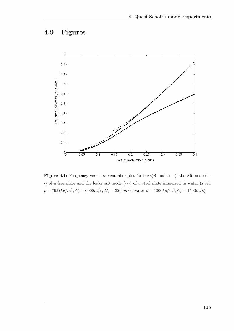
4. Quasi-Scholte mode Experiments
4.9 Figures
Figure 4.1: Frequency versus wavenumber plot for the QS mode (—), the A0 mode (- -
-) of a free plate and the leaky A0 mode (· · ·) of a steel plate immersed in water (steel:
ρ = 7932kg/m3, Cl = 6000m/s, Cs = 3260m/s; water ρ = 1000kg/m3, Cl = 1500m/s)
106
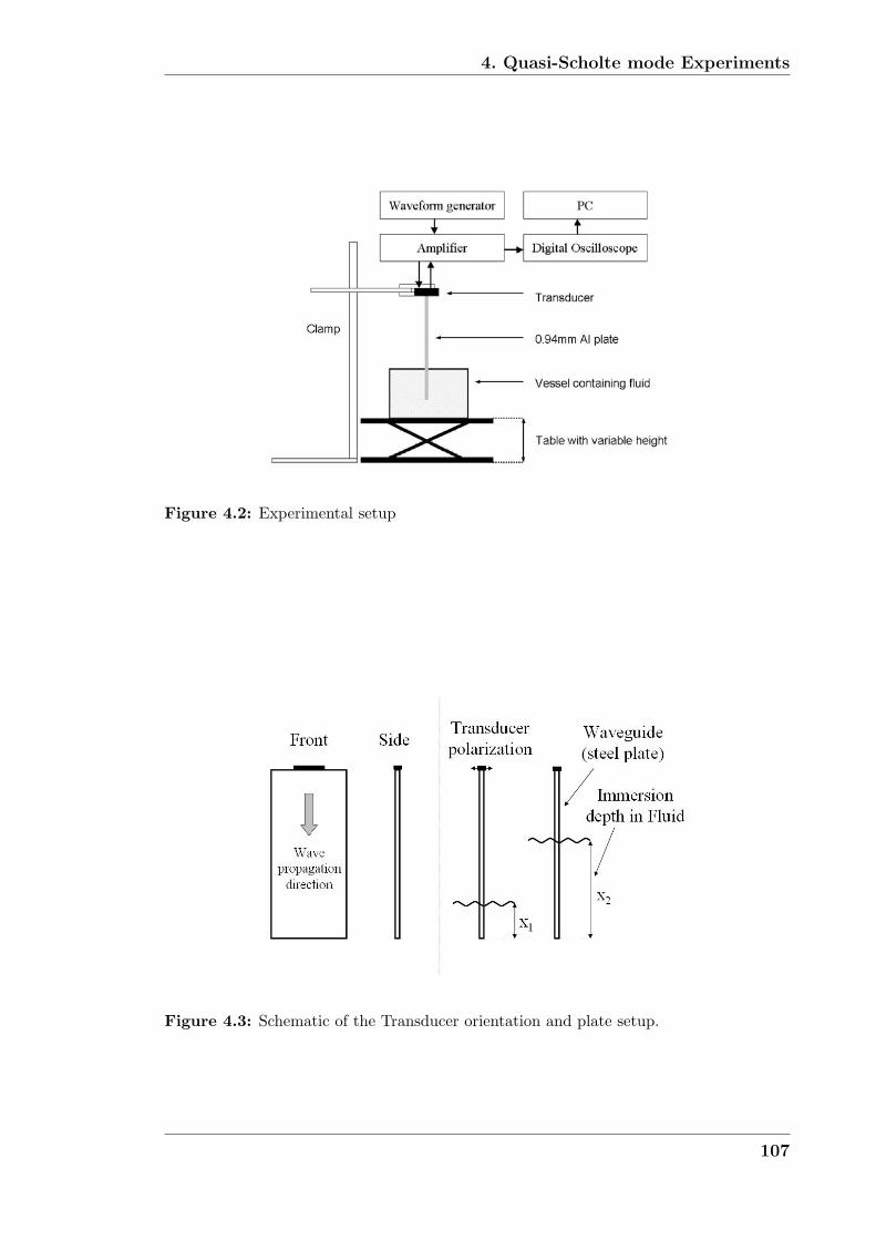
4. Quasi-Scholte mode Experiments
Figure 4.2: Experimental setup
Figure 4.3: Schematic of the Transducer orientation and plate setup.
107

4. Quasi-Scholte mode Experiments
Figure 4.4: Time trace at 500 kHz with aluminium plate 30 mm immersed in Glycerol
Figure 4.5: Time trace at 3 MHz with stainless steel plate immersed a) 20 mm and b)
80 mm in Water.
108

4. Quasi-Scholte mode Experiments
Figure 4.6: Schematic of a conventional test cell.
109
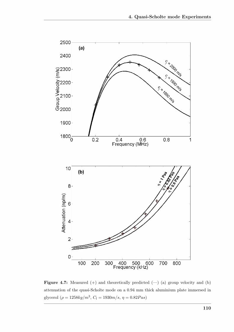
4. Quasi-Scholte mode Experiments
Figure 4.7: Measured (+) and theoretically predicted (—) (a) group velocity and (b)
attenuation of the quasi-Scholte mode on a 0.94 mm thick aluminium plate immersed in
glycerol (ρ = 1258kg/m3, Cl = 1930m/s, η = 0.82Pas)
110
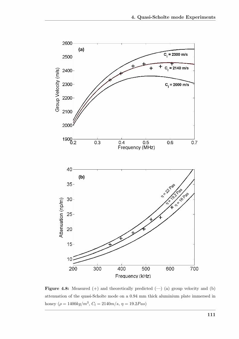
4. Quasi-Scholte mode Experiments
Figure 4.8: Measured (+) and theoretically predicted (—) (a) group velocity and (b)
attenuation of the quasi-Scholte mode on a 0.94 mm thick aluminium plate immersed in
honey (ρ = 1400kg/m3, Cl = 2140m/s, η = 19.2Pas)
111
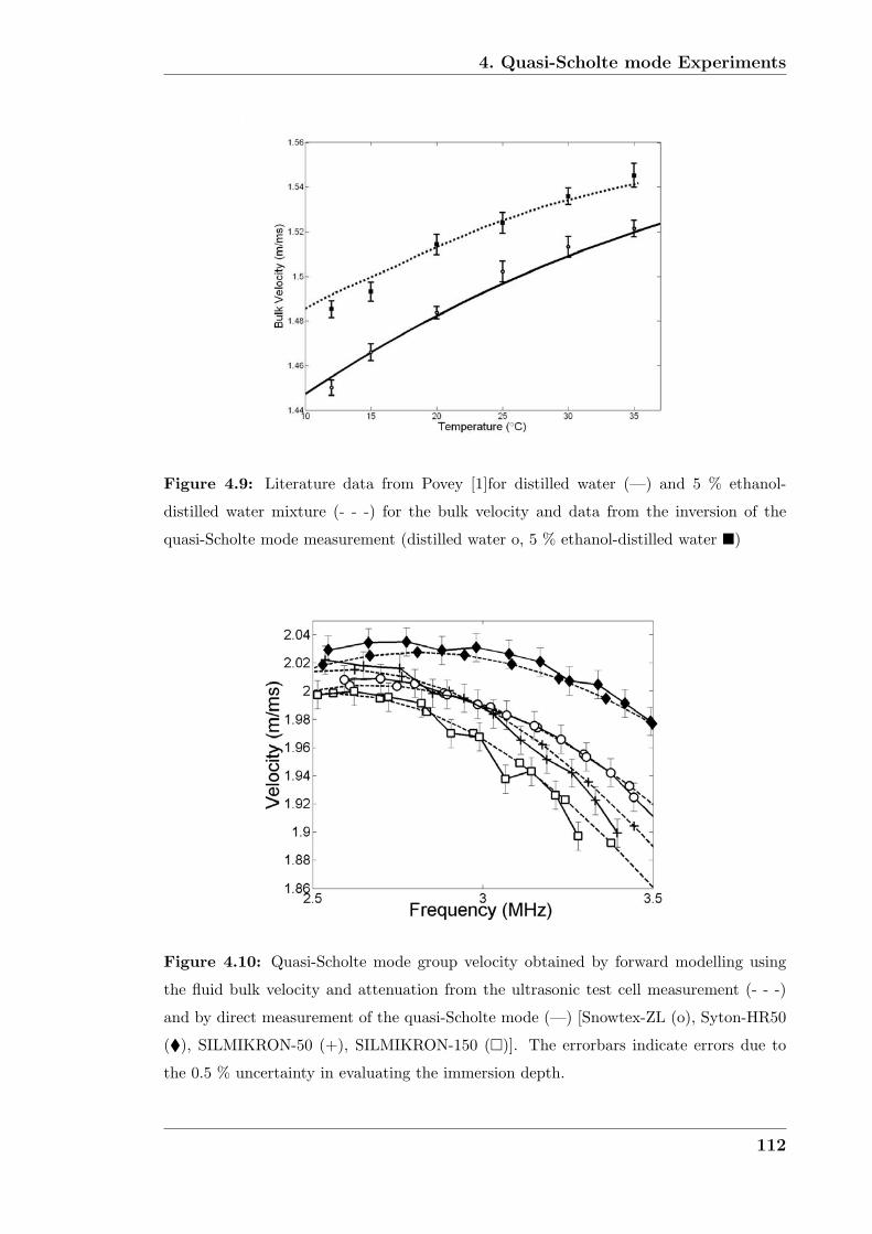
4. Quasi-Scholte mode Experiments
Figure 4.9: Literature data from Povey [1]for distilled water (—) and 5 % ethanol-
distilled water mixture (- - -) for the bulk velocity and data from the inversion of the
quasi-Scholte mode measurement (distilled water o, 5 % ethanol-distilled water �)
Figure 4.10: Quasi-Scholte mode group velocity obtained by forward modelling using
the fluid bulk velocity and attenuation from the ultrasonic test cell measurement (- - -)
and by direct measurement of the quasi-Scholte mode (—) [Snowtex-ZL (o), Syton-HR50
(�), SILMIKRON-50 (+), SILMIKRON-150 (�)]. The errorbars indicate errors due to
the 0.5 % uncertainty in evaluating the immersion depth.
112
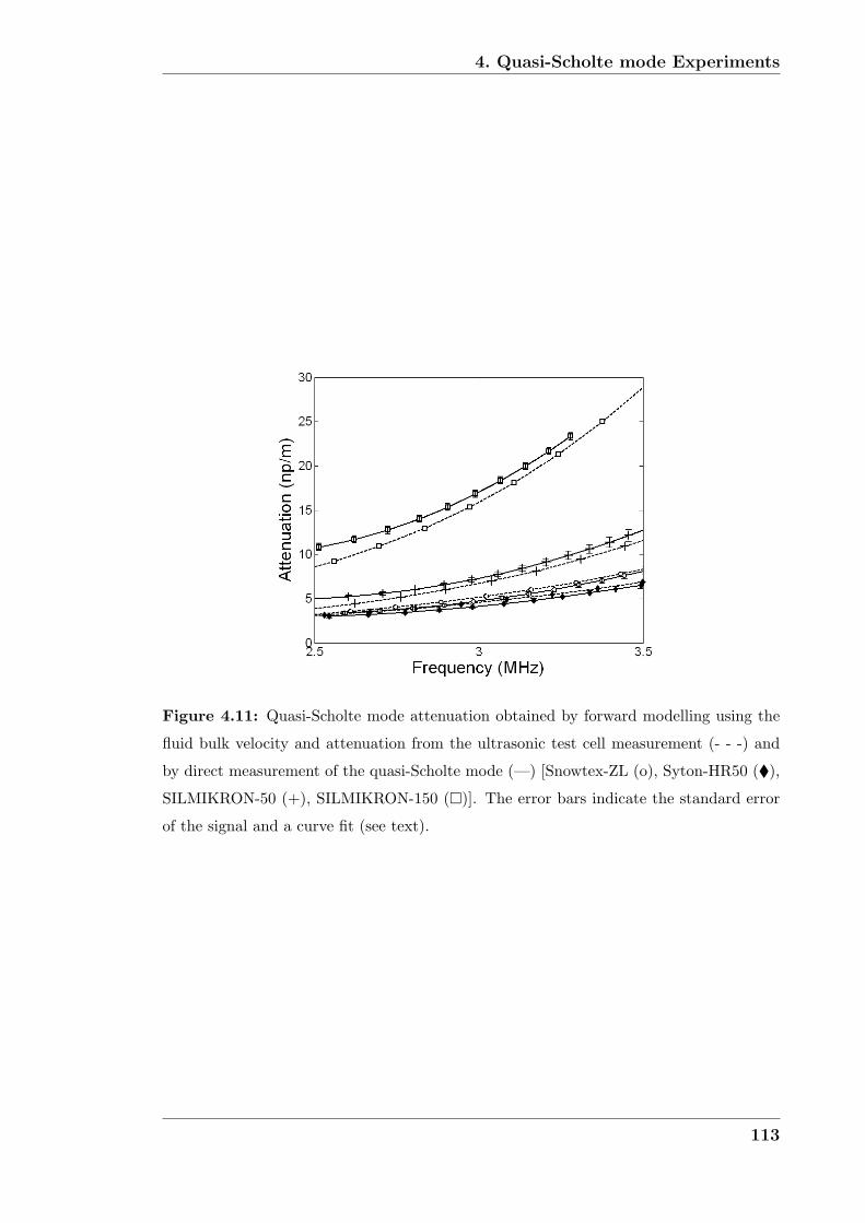
4. Quasi-Scholte mode Experiments
Figure 4.11: Quasi-Scholte mode attenuation obtained by forward modelling using the
fluid bulk velocity and attenuation from the ultrasonic test cell measurement (- - -) and
by direct measurement of the quasi-Scholte mode (—) [Snowtex-ZL (o), Syton-HR50 (�),
SILMIKRON-50 (+), SILMIKRON-150 (�)]. The error bars indicate the standard error
of the signal and a curve fit (see text).
113
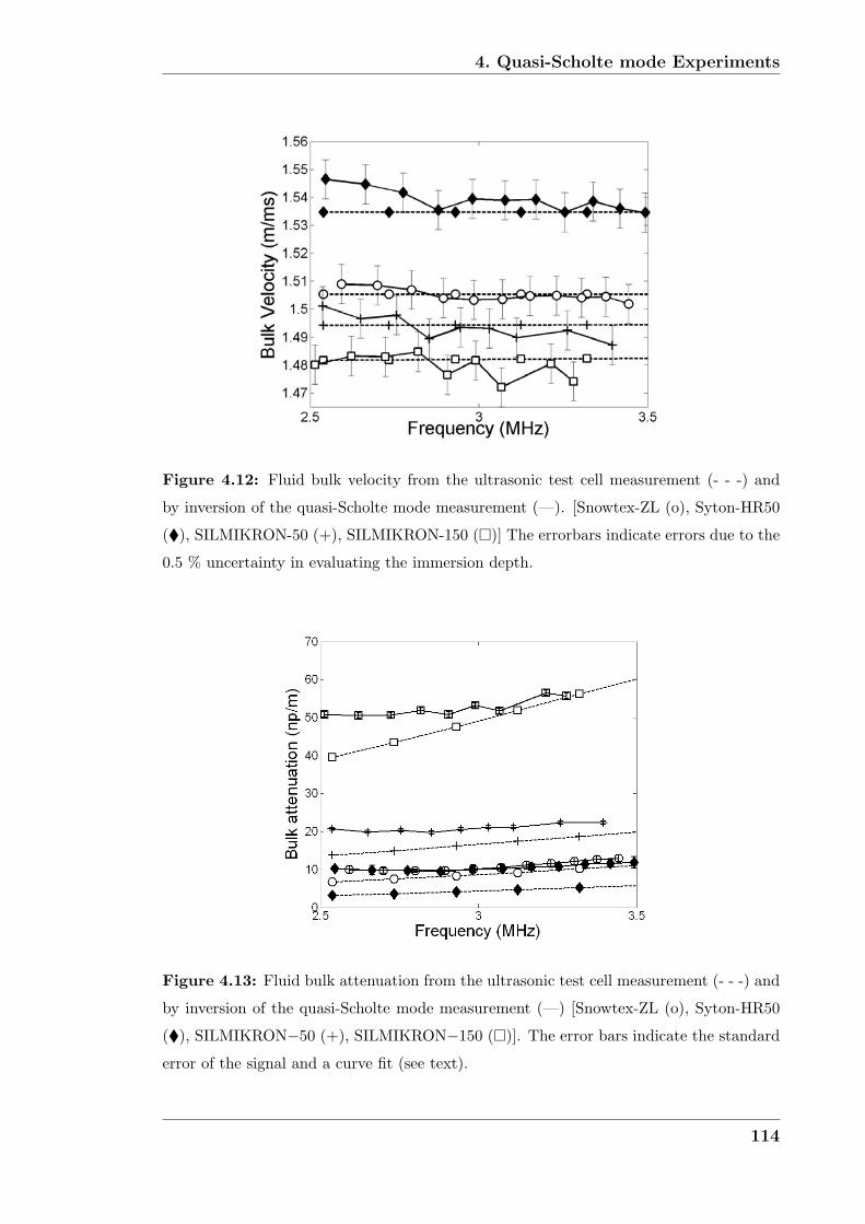
4. Quasi-Scholte mode Experiments
Figure 4.12: Fluid bulk velocity from the ultrasonic test cell measurement (- - -) and
by inversion of the quasi-Scholte mode measurement (—). [Snowtex-ZL (o), Syton-HR50
(�), SILMIKRON-50 (+), SILMIKRON-150 (�)] The errorbars indicate errors due to the
0.5 % uncertainty in evaluating the immersion depth.
Figure 4.13: Fluid bulk attenuation from the ultrasonic test cell measurement (- - -) and
by inversion of the quasi-Scholte mode measurement (—) [Snowtex-ZL (o), Syton-HR50
(�), SILMIKRON−50 (+), SILMIKRON−150 (�)]. The error bars indicate the standard
error of the signal and a curve fit (see text).
114
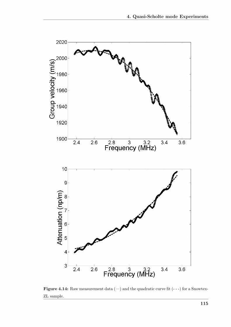
4. Quasi-Scholte mode Experiments
Figure 4.14: Raw measurement data (—) and the quadratic curve fit (- - -) for a Snowtex-
ZL sample.
115
Chapter 5
Non-dispersive wave propagation
in thin flexible waveguides
5.1 Shear horizontal mode
The work presented in chapters 3 and 4 suggested the investigation of propagating
modes in a strip of rectangular cross section. The search for a strip mode similar
to the A0 mode of an infinitely wide plate was started. It was hoped that this strip
mode could be used to excite a strip QS-mode, which was needed to further develop
the QS-mode measurement method and make it more practical.
During the investigation an A0-like mode was found and experimentally excited.
However during the analysis it was also found that non-dispersive ”shear horizon-
tal” like strip modes could easily be excited in strips of rectangular cross section.
It was realised that such a mode could be used to transmit ultrasonic energy from
a transducer through the strip waveguide to a structure non-dispersively and over
relatively long distances.
A non-dispersive waveguide has a high potential to be used in applications such as
ultrasonic thickness gauging or monitoring of cracks in structures at elevated tem-
peratures ( > 300◦C), in harsh environments or in places where access is limited.
116
5. Non-dispersive wave propagation in thin flexible waveguides
These tasks are straight forward for ultrasonic inspection equipment at room tem-
peratures or in safe environments. However in harsh environments such as the ones
described above, standard ultrasonic NDT equipment fails due to a number of rea-
sons, the most important being the loss of the transducer capabilities to send and
receive signals due to depolarisation of piezo electric materials at high temperatures
(Curie point of piezo-ceramics is typically about 250◦C) or under the influence of
high radiation levels.
Currently researchers are working on the development of transducer materials that
can withstand extreme conditions [4], [5]. The development and the manufacture
of these new materials is very expensive, therefore the alternative method of using
a waveguide to transmit energy from a standard transducer in a safe environment
into the structure at extreme conditions is very attractive. It was decided to focus
further research onto this field. The remainder of the work reported in this thesis
therefore concentrates on the development of an ”acoustic cable” for non-destructive
testing of a structure.
The main difficulties for the implementation of an ”acoustic cable” are the need for
an efficient excitation of a clean non- or marginally-dispersive signal and an attach-
ment to the structure that optimises transmission of a clean and strong signal into
the structure to be interrogated. These two tasks were separated. Wave propaga-
tion in waveguides is discussed in this chapter while the source characteristics of
waveguides on half-spaces are considered in chapter 6.
Whilst currently there exist no NDT devices for structural interrogation using a flex-
ible waveguide to separate the transducer from the test-piece, several publications
on non-dispersive waveguides and buffer rods for high temperature applications can
be found. These articles are mainly motivated by the field of fluid flow metering
where a strong signal needs to be sent across a fluid conduit. The flow velocity is
then evaluated by a change in transit time from a transducer on one side of the con-
duit to a receiver on the other side of the conduit. These embodiments of marginally
dispersive waveguides and their working principle will be outlined in section 5.3 af-
117
5. Non-dispersive wave propagation in thin flexible waveguides
ter a short section that highlights the desired wave propagation characteristics of
’acoustic cable’ buffer waveguides. Then wave propagation in strips of rectangular
cross section will be discussed. At the end of the chapter in section 5.5 experimental
work that has been carried out on rods, bundles of wires, wires and rectangular
strips is presented.
5.2 Desirable waveguide characteristics
There are several desirable characteristics that a waveguide should have for the
successful transmission of ultrasonic pulses from a transducer through the waveguide
into another structure. These characteristics will be discussed here. For this we recall
some of the basics of guided wave propagation which were described in section 2.2.
Single mode excitation
When examining figure 2.1 one notices that the number of propagating modes that
exist in a plate structure is large; indeed it is infinite, the higher the frequency of
operation the more modes exist. At any chosen frequency there are several modes
that can propagate. If two modes of similar velocity propagate in the plate their
signals will interfere or if the propagation distance is long enough, two separate ar-
rivals will be recorded. This will complicate the analysis of signals considerably if
the signals are close together. If more than a couple of modes propagate in the plate
it becomes nearly impossible to separate and differentiate the reflections and arrivals
of one mode from the signal arrivals of another mode. Therefore it is important to
limit the number of modes that propagate in a waveguide and ideally to use a single
pure mode to carry out testing.
The closer the transducer induced displacements match the mode shape of a mode,
the stronger this mode will be excited compared to other modes that do not match
the motion induced by the transducer. In a plate at low frequency thicknesses (<
1.7MHz mm) only three propagating modes exist. These fundamental modes have
distinct polarisation directions and can therefore rather easily be excited by applying
118
5. Non-dispersive wave propagation in thin flexible waveguides
a uniform displacement profile across the section of the plate in the direction of one
of the axes of the coordinate system (see 2.3). At higher frequencies, where higher
order modes are present and the mode shapes of the fundamental modes considerably
differ from a uniform profile across the plate thickness, it becomes more difficult to
excite a single mode. In these cases transduction methods using a wedge or comb
like transducers can be employed, see for example Monkhouse et al. [64]. However
for these reasons the traditional approach to single mode excitation is to operate at
low frequency thickness products.
In practice perfect excitation is not possible due to imperfections of the waveguide
or the transducer. However a single mode can be preferentially excited by certain
transducer configurations. Other modes will be excited at much lower amplitudes
and cause coherent noise. In general a good single mode excitation excites one mode
about 40 dB above other modes which allows satisfactory measurements.
Non-dispersiveness
In figure 2.2 the effects of dispersion are illustrated. Distortion and elongation of
the pulse shape decrease the spatial resolution with which an object could be mon-
itored and the amplitude loss due to dispersion considerably reduces the range of
the guided wave and therefore the length of a useable waveguide. Even though
techniques to counter the effects of dispersion exist with time reversal [28] and
dispersion compensation [27], these techniques complicate the method unnecessar-
ily and require excitation of complicated temporal signals and arbitrary waveform
generators. Therefore propagation in the waveguide should be non- or marginally-
dispersive. The traditional way of achieving this is to operate at low frequency
thicknesses; however if high spatial resolution and thus high frequencies are needed
the waveguide dimensions become very small.
Flexibility and low thickness
Apart from the cost savings and practical advantages that the use of a flexible and
thin waveguide entails, there is also a technical advantage due to the small dimen-
119
5. Non-dispersive wave propagation in thin flexible waveguides
sions of the waveguide. A thin waveguide is much better at isolating a transducer
from a hot environment than a larger cross section rod. This is illustrated in figure
5.1 where the temperature distribution along three different waveguides is plotted.
One end of each waveguide is attached to a hot (600◦C) structure while the other
end protrudes freely into surrounding air at room temperature (25◦C). The heat
transfer in the waveguide is modelled as described by Mills [65] for steady state
heat transfer along a fin. While the thin steel wave guides of characteristic dimen-
sion 1 mm ensure a temperature drop below 100◦C within 100 mm of length of the
waveguide, the thick rod of characteristic dimension 20mm only achieves a similar
temperature drop over 500mm of length.
Half a metre is a considerable clearance that the rigid larger diameter rod device
will need, while a thin, flexible waveguide can possibly be bent around corners to
reach into inaccessible areas.
Low attenuation and high corrosion resistance
The waveguide merely acts as a channel to send/receive the signal to and from an
area where it will interact with a structure to collect information. Ideally this should
occur without losses along the path that the signal is sent, therefore losses in the
waveguide should be minimised. In this respect longitudinal modes perform better
since they are attenuated less at high temperatures. According to Papadakis et al.
[66] there is no significant increase in the longitudinal or shear wave attenuation of
steel at 2MHz up to temperatures of ∼ 700◦C. Above 700◦C the shear wave at-
tenuation starts to increase considerably to about 0.5 Np/cm at 1100◦C, while the
longitudinal attenuation increases moderately and then reduces again to 0.1 Np/cm
at 1100◦C. However shear waves allow the use of lower frequencies for the same
resolution due to their slower wave velocity. Attenuation due to the grain size of the
material may also become important (see Reynolds and Smith [67]).
The waveguide material will also have to be robust enough to withstand an aggres-
sive environment and should be highly corrosion and radiation resistant. Therefore
stainless steel or ceramics are materials of choice for the waveguide.
120

5. Non-dispersive wave propagation in thin flexible waveguides
5.3 Non-dispersive waveguides in the literature
The work reported in the literature has mainly been motivated by the application
of flow monitoring of hot fluids in pipes. A substantial number of publications were
found to be in the form of patents. Lynnworth and co-workers [68], [69], [70] have
developed a series of wire bundle systems in order to produce marginally dispersive
propagation of extensional waves along a waveguide system. They identified disper-
sion as the main problem. In order to minimise dispersion in the waveguide they
excite the L(0, 1) mode in very thin wires. Due to the small diameter of the wires the
waveguide operates at low frequency thickness products where the phase velocity is
almost frequency independent and marginally dispersive, see section 2.6. In order
to obtain a strong signal many wires were put together in a bundle. Winston and
Brunk [71] have suggested a similar method using single or multiple wires, however
they did not specify any further information about an implementation of the method.
Heijnsdijk and van Klooster [72] have proposed a coiled foil waveguide as an alterna-
tive to a bundle of rods. The thickness of the foil is arranged to be much smaller than
the smallest wavelength to be propagated; this ensures that the frequency thickness
product of the foil is very low and therefore compressional pulses will essentially
propagate non-dispersively along the foil. The foil is coiled around an axis parallel
to the propagation direction and so if unwrapped would be very long in the direction
parallel to propagation. This mimics a plane wave propagating along the foil where
interferences from edges are kept to a minimum.
Jen and co-workers [73], [74], [75], [76] have tried to limit the number of modes
travelling in a thin bar by adding an attenuative cladding on the outside of the bar.
The bar can be of a tapered shape. It is essentially an attempt to remove the effects
of the waveguide boundaries mainly by damping and limiting the reflections of the
surface. The number of trailing echoes is thus almost entirely removed; however
the effects of dispersion are not entirely removed and the signal is slightly delayed,
slightly distorted and strongly attenuated. This method is an improvement to even
older solutions that utilise uniformly and non-uniformly threaded bars as waveg-
121
5. Non-dispersive wave propagation in thin flexible waveguides
uides [77], [78]. Nevertheless Jen’s method, like the threaded bars, suffers from high
attenuation over relatively short propagation distances. The relatively high attenu-
ation limits the propagation distance for this waveguide. At the same time a longer
waveguide is needed to isolate the transducer from high temperatures due to the
large diameter of the waveguide (see figure 5.1).
For the purpose of fluid flow metering Lynnworth [79] also patented a device that
he called the ”hockey stick”. It carries a shear wave in a rectangular section bar to
an angled section. The angle of the end of the ”hockey stick” is coupled to a pipe
wall in order to promote mode conversion from the shear wave to a compressional
wave in the liquid. On the other side of the pipe the compressional wave converts
back to a shear wave and is picked up in a similar device. A sketch of the ”hockey
stick” system for fluid flow metering is shown in figure 5.2.
5.4 Wave propagation in rectangular strips
The modelling of very wide plates is accurately achieved by the assumption of an
infinitely wide plate. The shorter the width of the plate/strip becomes the more
it starts influencing the wave propagation and it becomes necessary to model the
rectangular strip as a one dimensional waveguide with a constant cross section; a
family of modes can propagate along the waveguide. Mindlin and Fox [80] were
the first to describe the propagating modes of a bar of rectangular cross section.
Their solution was made up of a superposition of several flexural, longitudinal and
shear modes that propagate in infinite plates of the width and thickness of the bar
respectively. The solutions for the infinite plates were superposed in order to fulfil
the boundary conditions of zero stress all around the perimeter of the cross section.
This method enabled them to determine the dispersion characteristics of the bar
at distinct frequencies and aspect ratios of the bar. A solution for all frequencies
and aspect ratios was however not possible. More recently the continuous tracing of
dispersion curves for wave propagation in structures of arbitrary cross section has
become possible through the use of finite element (FE) eigensolvers. Wilcox et al.
122
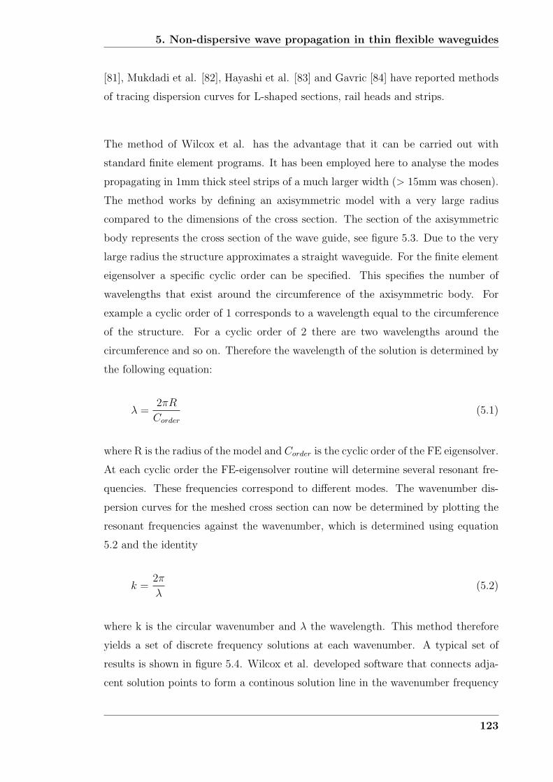
5. Non-dispersive wave propagation in thin flexible waveguides
[81], Mukdadi et al. [82], Hayashi et al. [83] and Gavric [84] have reported methods
of tracing dispersion curves for L-shaped sections, rail heads and strips.
The method of Wilcox et al. has the advantage that it can be carried out with
standard finite element programs. It has been employed here to analyse the modes
propagating in 1mm thick steel strips of a much larger width (> 15mm was chosen).
The method works by defining an axisymmetric model with a very large radius
compared to the dimensions of the cross section. The section of the axisymmetric
body represents the cross section of the wave guide, see figure 5.3. Due to the very
large radius the structure approximates a straight waveguide. For the finite element
eigensolver a specific cyclic order can be specified. This specifies the number of
wavelengths that exist around the circumference of the axisymmetric body. For
example a cyclic order of 1 corresponds to a wavelength equal to the circumference
of the structure. For a cyclic order of 2 there are two wavelengths around the
circumference and so on. Therefore the wavelength of the solution is determined by
the following equation:
λ =2πR
Corder
(5.1)
where R is the radius of the model and Corder is the cyclic order of the FE eigensolver.
At each cyclic order the FE-eigensolver routine will determine several resonant fre-
quencies. These frequencies correspond to different modes. The wavenumber dis-
persion curves for the meshed cross section can now be determined by plotting the
resonant frequencies against the wavenumber, which is determined using equation
5.2 and the identity
k =2π
λ(5.2)
where k is the circular wavenumber and λ the wavelength. This method therefore
yields a set of discrete frequency solutions at each wavenumber. A typical set of
results is shown in figure 5.4. Wilcox et al. developed software that connects adja-
cent solution points to form a continous solution line in the wavenumber frequency
123
5. Non-dispersive wave propagation in thin flexible waveguides
domain. This represents a mode. The joining up of adjacent points to a line is car-
ried out by comparing the mode shapes of adjacent solutions and by using the slope
of the curve of existing solutions to predict the continuation of the curve, which is
similar to the method presented by Lowe [23]. A software coding of this had been
developed by Wilcox and was merely used here to extract results for the desired
geometries. The finite element software that determined the eigen solutions was the
FINEL 77 code which was developed by Hitchings [85] at Imperial College.
Phase velocity dispersion curves can be obtained from the wavenumber frequency
plot by converting them using the following identity:
Cph =ω
k(5.3)
Once the phase velocity is determined the group velocity can be calculated using:
Cgr =∂ω
∂k= Cph + k
∂Cph
∂k(5.4)
An interesting aspect to note about the technique is that the determined FE eigen
solutions are confined to a rectangular domain in the frequency - wavenumber
space. However when this is transformed into a phase velocity - frequency space
the solutions will be bound in a space between the two lines Cph = (1/kmin)ω and
Cph = (1/kmax)ω. This is illustrated in figure 5.5.
The mode shapes of each mode are a direct result of the FE analysis and can be
extracted at each frequency.
5.4.1 Dispersion curves for rectangular strips
Using the technique described in the previous section dispersion curves for rectan-
gular strips were obtained. The results for steel (ρ = 7932kg/m3, E = 216.9GPa,
ν = 0.2865) strip geometries of 1 mm thickness and width 15 and 30 mm will be
presented here. A sketch of the finite element model that was defined is shown in
figure 5.3. After the finite element program (FINEL 77 [85]) was run the data was
124
5. Non-dispersive wave propagation in thin flexible waveguides
post processed using the codes developed by Wilcox et al. [81]. Figure 5.6 shows the
frequency-wavenumber and phase velocity-frequency dispersion curves. The figure
looks very busy because many more propagating modes exist at lower frequencies
than in the infinite plate case. These extra modes are mainly due to the finite width
of the strip.
In figure 5.6 two modes are highlighted. These modes were named A0* and SH*.
The A0* mode is very similar to the commonly known A0 mode in an infinite plate.
It is a flexural mode with respect to the thickness (x direction), however due to the
finite width the mode also has a variation across the width (y direction). In this
case the mode is symmetric about the width with maximum displacement at the
centre of the rectangular strip. The relationship of the mode to the A0 mode in an
infinite plate is underlined by their similarity in phase velocity. Figure 5.7 shows the
mode shape of the A0* mode at 2.5 MHz. The main displacement component is in
the x direction and displacements are concentrated at the centre of the strip. This
is the strip mode that would preferentially be excited to promote mode conversion
to a QS-strip mode and carry out fluid property measurements similar to those in
chapters 3 and 4.
The SH* mode was identified as the lowest order shear horizontal mode that exists
in the rectangular strip. Strictly speaking the term ’shear horizontal’ only makes
sense if the plate is infinite. Here the width is much larger than the thickness of the
plate and therefore ’shear horizontal’ mode refers to a mode with similar polarisa-
tion to an SH mode in the infinite plate. The same mode could also be described
as bending in the width-propagation direction plane. Shearing with respect to the
thickness of the strip is bending with respect to the width of the strip. An equivalent
to the SH0 mode in an infinite plate does not exist in a strip. The SH* mode has a
cut-off that depends on the width of the strip. At frequencies well above the cut-off
the mode asymptotes to the shear velocity of the strip. The mode shapes of the
SH* mode at different frequencies are shown in figure 5.8. The figure shows that at
high frequencies the y displacement component is dominant and concentrated in the
centre of the strip. The mode shape is constant across the x direction. Also near
125
5. Non-dispersive wave propagation in thin flexible waveguides
cut-off there are displacements at the edges of the strip. This is better illustrated
in figure 5.9 which shows the evolution of the dominant y displacement across the
width of the strip over a range of frequencies.
The influence of the shape of the excitation at the end section of the strip was investi-
gated in order to find the best way to excite the SH* mode strongly. A finite element
model for a 15mm wide steel strip was prepared in the ABAQUS finite element soft-
ware. The model was two dimensional with a plane stress condition in the thickness
direction of the strip. Due to its special polarisation the SH* mode only contains σzy
stress components, which satisfy the plane stress condition (σxx = σxy = σxz = 0).
A frequency domain solver was used to solve the problem. At one end of the strip
a steady, dynamic force was applied while an absorbing region at the other end of
the strip prevented any reflections of the excited waves.
A sketch of the FE model is displayed in figure 5.10. Square quadratic elements of
size 0.25mm were used to mesh the strip and the absorbing region. The viscoelas-
tic parameters of the absorbing region were increased in a cubic fashion from the
interface with the strip. They were determined as described by Drodz et al. [86].
Different distributions of exciting force over the width of the steel strip (ρ = 7932
kg/m3, E = 216.9 GPa, ν = 0.2865) were used to see the influence of the excitation
force profile on the excited waves in the strip.
The results of the FE analysis are displayed in figure 5.11. In the figure three differ-
ent profiles of excitation force across the width are shown as well as the y (width)
direction displacement field that they produce. For a uniformly applied force the
displacement field (figure 5.11a ) in the strip becomes relatively complicated. It can
be concluded that many modes are excited and interfere. If the stress profile of the
SH* mode (from the FE eigensolver) is applied at the strip end (figure 5.11b ), a
pure mode can be excited in the strip. Displacements are concentrated at the centre
of the strip. For a triangular forcing profile, the SH* mode is also preferentially
excited (figure 5.11c ). However some other modes are also excited so that the dis-
placement field in the strip is not as uniform as in the case of the exact mode shape
126
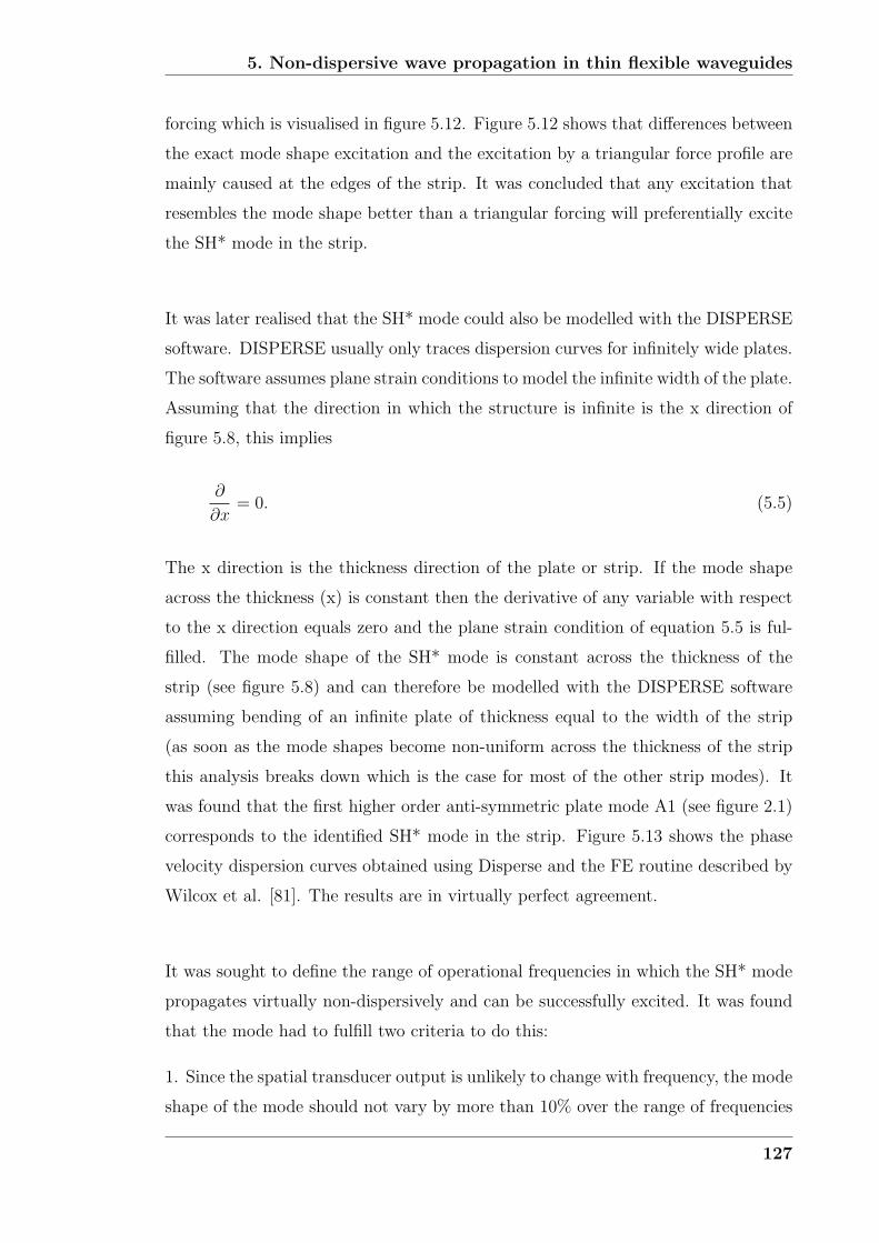
5. Non-dispersive wave propagation in thin flexible waveguides
forcing which is visualised in figure 5.12. Figure 5.12 shows that differences between
the exact mode shape excitation and the excitation by a triangular force profile are
mainly caused at the edges of the strip. It was concluded that any excitation that
resembles the mode shape better than a triangular forcing will preferentially excite
the SH* mode in the strip.
It was later realised that the SH* mode could also be modelled with the DISPERSE
software. DISPERSE usually only traces dispersion curves for infinitely wide plates.
The software assumes plane strain conditions to model the infinite width of the plate.
Assuming that the direction in which the structure is infinite is the x direction of
figure 5.8, this implies
∂
∂x= 0. (5.5)
The x direction is the thickness direction of the plate or strip. If the mode shape
across the thickness (x) is constant then the derivative of any variable with respect
to the x direction equals zero and the plane strain condition of equation 5.5 is ful-
filled. The mode shape of the SH* mode is constant across the thickness of the
strip (see figure 5.8) and can therefore be modelled with the DISPERSE software
assuming bending of an infinite plate of thickness equal to the width of the strip
(as soon as the mode shapes become non-uniform across the thickness of the strip
this analysis breaks down which is the case for most of the other strip modes). It
was found that the first higher order anti-symmetric plate mode A1 (see figure 2.1)
corresponds to the identified SH* mode in the strip. Figure 5.13 shows the phase
velocity dispersion curves obtained using Disperse and the FE routine described by
Wilcox et al. [81]. The results are in virtually perfect agreement.
It was sought to define the range of operational frequencies in which the SH* mode
propagates virtually non-dispersively and can be successfully excited. It was found
that the mode had to fulfill two criteria to do this:
1. Since the spatial transducer output is unlikely to change with frequency, the mode
shape of the mode should not vary by more than 10% over the range of frequencies
127

5. Non-dispersive wave propagation in thin flexible waveguides
contained within the excitation signal.
2. In order to guarantee very low levels of dispersion the phase velocity of the mode
should not vary by more than 2% over the range of frequencies contained within the
excitation signal.
By analysing the phase velocity dispersion curves and the mode shape of the SH*
mode it was found that these criteria are fulfilled above a frequency-width product
of 15MHz mm for a steel strip. To make this condition independent of the material
the frequency width was normalised by the shear wavelength of the material. The
shear wavelength of a 1 MHz signal in steel is approximately 3mm. The strip has
to be 15mm wide at 1MHz to fulfill the above conditions. Therefore the width of
a 1 mm thick strip has to be at least 5 bulk shear wavelengths to ensure the pos-
sibility of exciting a virtually non dispersive SH* mode. It can be concluded that
if a broadband signal is excited the width of the strip has to be larger than 5 bulk
shear wavelengths of the lowest frequency component contained within the signal.
While this criterion is true for the SH* mode in waveguides of any thickness as long
as the mode shape is constant across the thickness, thin waveguides of thicknesses
less than a shear bulk wavelength are more flexible, cheaper and more practical.
5.5 Experimental work and preferential excita-
tion of a single mode
Initially experiments on rods and wires were carried out. The traditional route of
minimising the frequency-radius product to achieve non-dispersive propagation was
employed. This had the advantage of limiting the number of propagating modes
in the wire to the fundamental three modes which can easily be excited selectively
by choosing appropriate transduction methods. At low frequency-radius products
this also makes wave propagation virtually non-dispersive for the L(0, 1) mode, the
T(0, 1) mode being non-dispersive anyway. Since excitation of the T(0, 1) mode
at high frequencies becomes difficult with standard transducers (due to the short
wavelength), experiments were focused on the L(0, 1) mode which could be excited
128
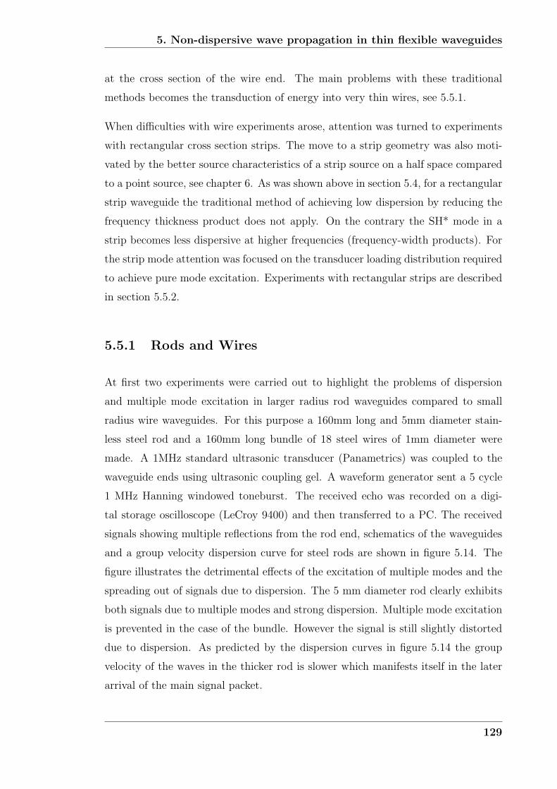
5. Non-dispersive wave propagation in thin flexible waveguides
at the cross section of the wire end. The main problems with these traditional
methods becomes the transduction of energy into very thin wires, see 5.5.1.
When difficulties with wire experiments arose, attention was turned to experiments
with rectangular cross section strips. The move to a strip geometry was also moti-
vated by the better source characteristics of a strip source on a half space compared
to a point source, see chapter 6. As was shown above in section 5.4, for a rectangular
strip waveguide the traditional method of achieving low dispersion by reducing the
frequency thickness product does not apply. On the contrary the SH* mode in a
strip becomes less dispersive at higher frequencies (frequency-width products). For
the strip mode attention was focused on the transducer loading distribution required
to achieve pure mode excitation. Experiments with rectangular strips are described
in section 5.5.2.
5.5.1 Rods and Wires
At first two experiments were carried out to highlight the problems of dispersion
and multiple mode excitation in larger radius rod waveguides compared to small
radius wire waveguides. For this purpose a 160mm long and 5mm diameter stain-
less steel rod and a 160mm long bundle of 18 steel wires of 1mm diameter were
made. A 1MHz standard ultrasonic transducer (Panametrics) was coupled to the
waveguide ends using ultrasonic coupling gel. A waveform generator sent a 5 cycle
1 MHz Hanning windowed toneburst. The received echo was recorded on a digi-
tal storage oscilloscope (LeCroy 9400) and then transferred to a PC. The received
signals showing multiple reflections from the rod end, schematics of the waveguides
and a group velocity dispersion curve for steel rods are shown in figure 5.14. The
figure illustrates the detrimental effects of the excitation of multiple modes and the
spreading out of signals due to dispersion. The 5 mm diameter rod clearly exhibits
both signals due to multiple modes and strong dispersion. Multiple mode excitation
is prevented in the case of the bundle. However the signal is still slightly distorted
due to dispersion. As predicted by the dispersion curves in figure 5.14 the group
velocity of the waves in the thicker rod is slower which manifests itself in the later
arrival of the main signal packet.
129

5. Non-dispersive wave propagation in thin flexible waveguides
The signal transmission from the transducer into the rod and bundle was very inef-
ficient and the detected signals were very weak. It was also attempted to bond piezo
ceramic elements directly to the bundle using adhesive. This was known to work
well at low frequency in a solid rod. However due to the relatively large diameter of
the piezo ceramic discs, radial resonances in the disc were excited at high frequen-
cies and the discs proved to be useless for L(0, 1) excitation in the wire bundle. An
attempt was then made to isolate a single wire in order to excite a strong signal in
the single wire. Two possible ways of achieving this were:
1. the amplification of the signal of a standard ultrasonic transducer by means of a
horn
2. the direct bonding of a piezo electric disc of the diameter of the wire to the end
of the wire.
Nicholson and McDicken [87] have reported experimental trials to transmit ultra-
sonic energy via a horn into wires. They tried several different shapes of horns and
did transmit energy through the horn into the wires. However the signal shapes
were severely distorted and signs of excitation of multiple modes in the wires were
shown. Tang and Lau [88] modelled sound transmission through a non-uniform
section, similar to a taper, and also concluded that the transmitted signal is very
complicated and hard to predict.
Both the above studies were carried out at frequencies where the wavelength of the
wave is considerably smaller than the dimension of the cross section. The author
believes that this was the cause of the problem. Many modes can exist across the
large diameter of the taper and therefore a distorted and complicated multi mode
signal is transmitted into the wire. A possible remedy for this problem was thought
to be the use of a hollow tapered section, similar to a funnel, that would connect
the transducer to the wire. The wall thickness of the funnel would be chosen to be
much smaller than a wavelength. Finite element simulations of propagation from
the tapered hollow section to the wire initially showed good results and minimal
signal distortion. However the manufacture of a thin hollow tapered section was
found to be difficult and since a wire point source on a half space was found to be
130
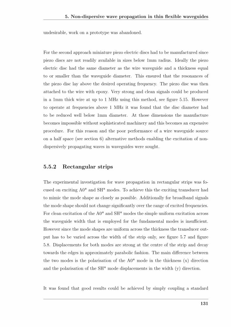
5. Non-dispersive wave propagation in thin flexible waveguides
undesirable, work on a prototype was abandoned.
For the second approach miniature piezo electric discs had to be manufactured since
piezo discs are not readily available in sizes below 1mm radius. Ideally the piezo
electric disc had the same diameter as the wire waveguide and a thickness equal
to or smaller than the waveguide diameter. This ensured that the resonances of
the piezo disc lay above the desired operating frequency. The piezo disc was then
attached to the wire with epoxy. Very strong and clean signals could be produced
in a 1mm thick wire at up to 1 MHz using this method, see figure 5.15. However
to operate at frequencies above 1 MHz it was found that the disc diameter had
to be reduced well below 1mm diameter. At those dimensions the manufacture
becomes impossible without sophisticated machinery and this becomes an expensive
procedure. For this reason and the poor performance of a wire waveguide source
on a half space (see section 6) alternative methods enabling the excitation of non-
dispersively propagating waves in waveguides were sought.
5.5.2 Rectangular strips
The experimental investigation for wave propagation in rectangular strips was fo-
cused on exciting A0* and SH* modes. To achieve this the exciting transducer had
to mimic the mode shape as closely as possible. Additionally for broadband signals
the mode shape should not change significantly over the range of excited frequencies.
For clean excitation of the A0* and SH* modes the simple uniform excitation across
the waveguide width that is employed for the fundamental modes is insufficient.
However since the mode shapes are uniform across the thickness the transducer out-
put has to be varied across the width of the strip only, see figure 5.7 and figure
5.8. Displacements for both modes are strong at the centre of the strip and decay
towards the edges in approximately parabolic fashion. The main difference between
the two modes is the polarisation of the A0* mode in the thickness (x) direction
and the polarisation of the SH* mode displacements in the width (y) direction.
It was found that good results could be achieved by simply coupling a standard
131
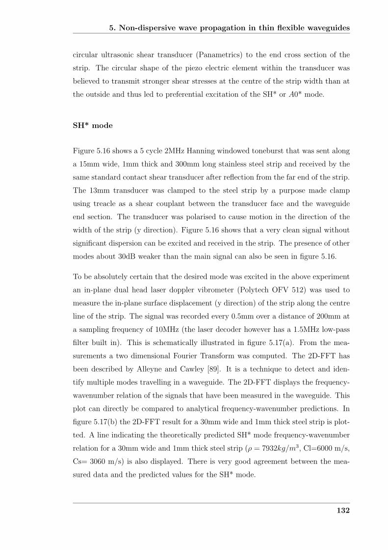
5. Non-dispersive wave propagation in thin flexible waveguides
circular ultrasonic shear transducer (Panametrics) to the end cross section of the
strip. The circular shape of the piezo electric element within the transducer was
believed to transmit stronger shear stresses at the centre of the strip width than at
the outside and thus led to preferential excitation of the SH* or A0* mode.
SH* mode
Figure 5.16 shows a 5 cycle 2MHz Hanning windowed toneburst that was sent along
a 15mm wide, 1mm thick and 300mm long stainless steel strip and received by the
same standard contact shear transducer after reflection from the far end of the strip.
The 13mm transducer was clamped to the steel strip by a purpose made clamp
using treacle as a shear couplant between the transducer face and the waveguide
end section. The transducer was polarised to cause motion in the direction of the
width of the strip (y direction). Figure 5.16 shows that a very clean signal without
significant dispersion can be excited and received in the strip. The presence of other
modes about 30dB weaker than the main signal can also be seen in figure 5.16.
To be absolutely certain that the desired mode was excited in the above experiment
an in-plane dual head laser doppler vibrometer (Polytech OFV 512) was used to
measure the in-plane surface displacement (y direction) of the strip along the centre
line of the strip. The signal was recorded every 0.5mm over a distance of 200mm at
a sampling frequency of 10MHz (the laser decoder however has a 1.5MHz low-pass
filter built in). This is schematically illustrated in figure 5.17(a). From the mea-
surements a two dimensional Fourier Transform was computed. The 2D-FFT has
been described by Alleyne and Cawley [89]. It is a technique to detect and iden-
tify multiple modes travelling in a waveguide. The 2D-FFT displays the frequency-
wavenumber relation of the signals that have been measured in the waveguide. This
plot can directly be compared to analytical frequency-wavenumber predictions. In
figure 5.17(b) the 2D-FFT result for a 30mm wide and 1mm thick steel strip is plot-
ted. A line indicating the theoretically predicted SH* mode frequency-wavenumber
relation for a 30mm wide and 1mm thick steel strip (ρ = 7932kg/m3, Cl=6000 m/s,
Cs= 3060 m/s) is also displayed. There is very good agreement between the mea-
sured data and the predicted values for the SH* mode.
132
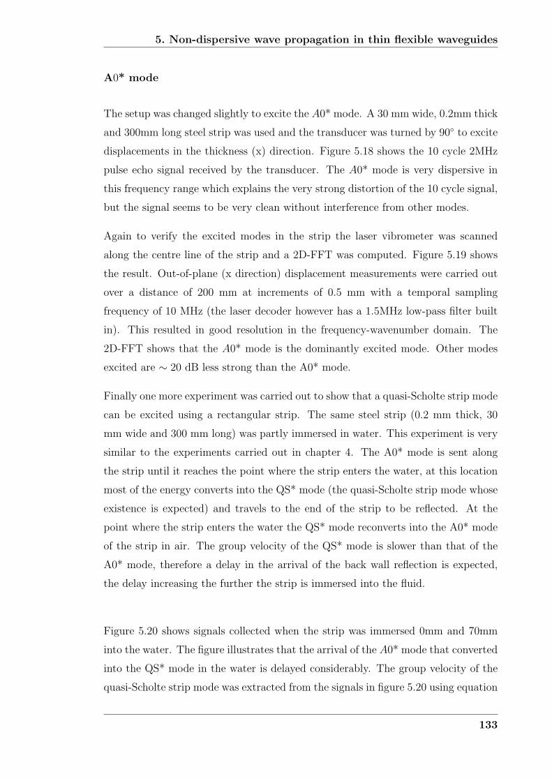
5. Non-dispersive wave propagation in thin flexible waveguides
A0* mode
The setup was changed slightly to excite the A0* mode. A 30 mm wide, 0.2mm thick
and 300mm long steel strip was used and the transducer was turned by 90◦ to excite
displacements in the thickness (x) direction. Figure 5.18 shows the 10 cycle 2MHz
pulse echo signal received by the transducer. The A0* mode is very dispersive in
this frequency range which explains the very strong distortion of the 10 cycle signal,
but the signal seems to be very clean without interference from other modes.
Again to verify the excited modes in the strip the laser vibrometer was scanned
along the centre line of the strip and a 2D-FFT was computed. Figure 5.19 shows
the result. Out-of-plane (x direction) displacement measurements were carried out
over a distance of 200 mm at increments of 0.5 mm with a temporal sampling
frequency of 10 MHz (the laser decoder however has a 1.5MHz low-pass filter built
in). This resulted in good resolution in the frequency-wavenumber domain. The
2D-FFT shows that the A0* mode is the dominantly excited mode. Other modes
excited are ∼ 20 dB less strong than the A0* mode.
Finally one more experiment was carried out to show that a quasi-Scholte strip mode
can be excited using a rectangular strip. The same steel strip (0.2 mm thick, 30
mm wide and 300 mm long) was partly immersed in water. This experiment is very
similar to the experiments carried out in chapter 4. The A0* mode is sent along
the strip until it reaches the point where the strip enters the water, at this location
most of the energy converts into the QS* mode (the quasi-Scholte strip mode whose
existence is expected) and travels to the end of the strip to be reflected. At the
point where the strip enters the water the QS* mode reconverts into the A0* mode
of the strip in air. The group velocity of the QS* mode is slower than that of the
A0* mode, therefore a delay in the arrival of the back wall reflection is expected,
the delay increasing the further the strip is immersed into the fluid.
Figure 5.20 shows signals collected when the strip was immersed 0mm and 70mm
into the water. The figure illustrates that the arrival of the A0* mode that converted
into the QS* mode in the water is delayed considerably. The group velocity of the
quasi-Scholte strip mode was extracted from the signals in figure 5.20 using equation
133
5. Non-dispersive wave propagation in thin flexible waveguides
4.1. The DISPERSE software was also used to predict the quasi-Scholte mode group
velocity for an infinite plate immersed in water. The measurement and prediction
are shown in figure 5.21. The result suggest that the rectangular strip A0* mode
can be used to excite a quasi-Scholte strip mode when the strip is partly immersed
in water. The behaviour also seems to be similar to the infinite plate case.
5.6 Summary
In this chapter wave propagation in waveguides of different geometries was dis-
cussed. The work was initially motivated by the search for a suitable A0 like mode
in a rectangular strip which could be used to excite a QS strip mode for fluid char-
acterisation. When the modes of a rectangular strip were analysed a marginally
dispersive shear horizontal type mode was found. The potential of this mode in
applications like ultrasonic buffer waveguides was realised and research was diverted
towards the development of an ’acoustic cable’ waveguide system that allows the
transmission of ultrasonic energy from a transducer in a safe environment to an
object that is to be interrogated in a harsh environment or a place where access is
limited.
It was found that to date publications report a reasonable amount of work that
has been carried out on the subject of non-dispersive waveguides. Most of this
work was motivated by the need for high temperature flow measurements. In the
published work the major problems of dispersion and presence of multiple modes
were overcome by working at low frequency thickness/radius products. The use
of the SH* strip mode that is suggested here differs from the traditional methods
since it is non-dispersive at high frequency thickness (width) products. The mode
can be selectively excited due to its distinct mode shape that is concentrated in
the centre of the strip. Some experimental results for the traditional low frequency
radius regime excitation of signals in cylindrical structures were presented. The
experimental excitation of the SH* mode was also demonstrated. With the current
transduction method in the pulse echo mode the SH* mode could be excited and
received at least 30dB stronger than other modes of the strip.
134
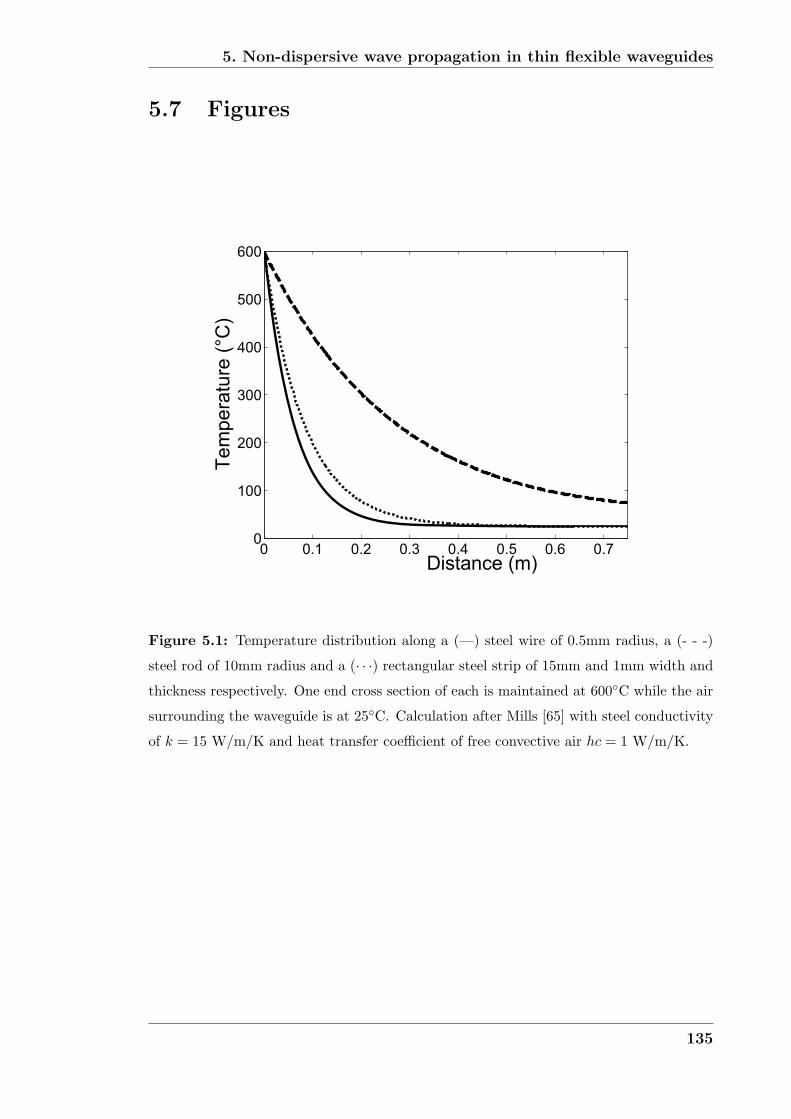
5. Non-dispersive wave propagation in thin flexible waveguides
5.7 Figures
0 0.1 0.2 0.3 0.4 0.5 0.6 0.70
100
200
300
400
500
600
Distance (m)
Te
mp
era
ture
(°C
)
Figure 5.1: Temperature distribution along a (—) steel wire of 0.5mm radius, a (- - -)
steel rod of 10mm radius and a (· · ·) rectangular steel strip of 15mm and 1mm width and
thickness respectively. One end cross section of each is maintained at 600◦C while the air
surrounding the waveguide is at 25◦C. Calculation after Mills [65] with steel conductivity
of k = 15 W/m/K and heat transfer coefficient of free convective air hc = 1 W/m/K.
135
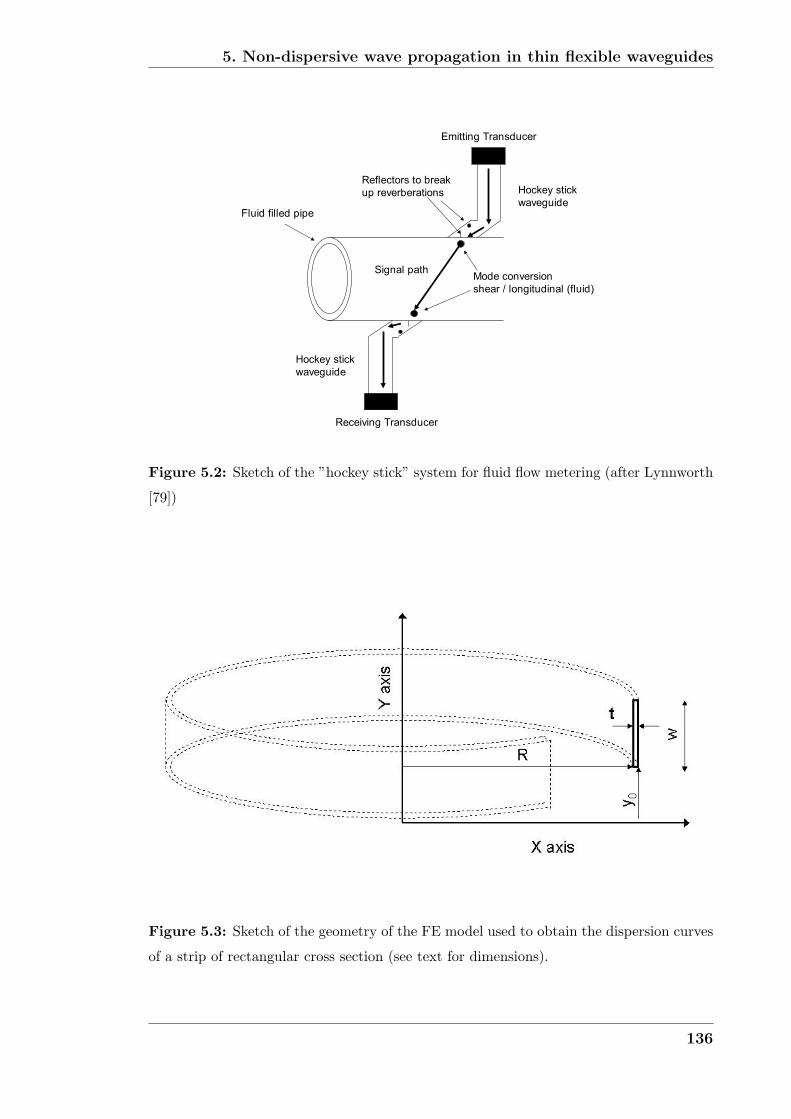
5. Non-dispersive wave propagation in thin flexible waveguides
� �
������������ ����
������������
������� ��
������������
������� ��
������������� ����
�����������������
���������������
������������
���� ������ ������
�� ������������
����� �������� �����!���� "�
Figure 5.2: Sketch of the ”hockey stick” system for fluid flow metering (after Lynnworth
[79])
Figure 5.3: Sketch of the geometry of the FE model used to obtain the dispersion curves
of a strip of rectangular cross section (see text for dimensions).
136
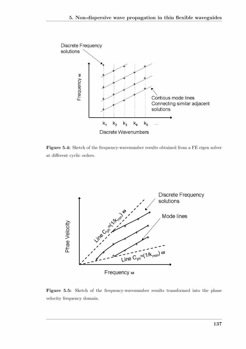
5. Non-dispersive wave propagation in thin flexible waveguides
Figure 5.4: Sketch of the frequency-wavenumber results obtained from a FE eigen solver
at different cyclic orders.
Figure 5.5: Sketch of the frequency-wavenumber results transformed into the phase
velocity frequency domain.
137
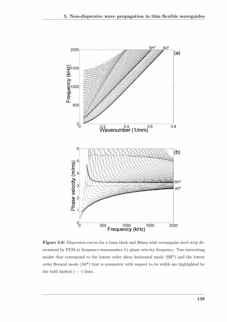
5. Non-dispersive wave propagation in thin flexible waveguides
Figure 5.6: Dispersion curves for a 1mm thick and 30mm wide rectangular steel strip de-
termined by FEM a) frequency-wavenumber b) phase velocity frequency. Two interesting
modes that correspond to the lowest order shear horizontal mode (SH*) and the lowest
order flexural mode (A0*) that is symmetric with respect to its width are highlighted by
the bold dashed (- - -) lines.
138
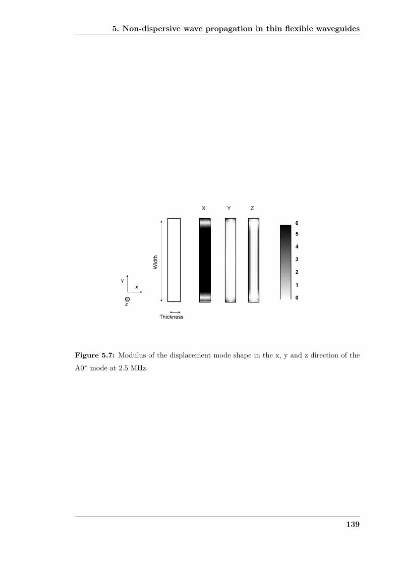
5. Non-dispersive wave propagation in thin flexible waveguides
� �
�
�
�
�� �� ��
�
�
�
��� ��
����
�
�
�
�
Figure 5.7: Modulus of the displacement mode shape in the x, y and z direction of the
A0* mode at 2.5 MHz.
139
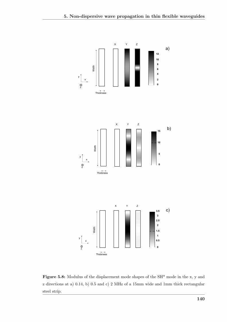
5. Non-dispersive wave propagation in thin flexible waveguides
� �
�
�
�
�� �� ��
��
�
�
��� ������
��
�
�
�
��
� �
�
�
�
�� �� ��
��
�
�
��� ��
����
����
� �
��
�
�� �� �
�
���
�
���
�
���
�
�� ����
����
��� ��
Figure 5.8: Modulus of the displacement mode shapes of the SH* mode in the x, y and
z directions at a) 0.14, b) 0.5 and c) 2 MHz of a 15mm wide and 1mm thick rectangular
steel strip.
140
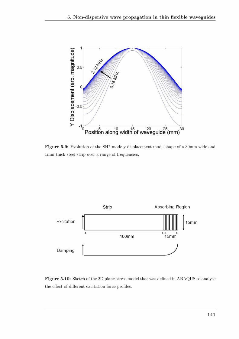
5. Non-dispersive wave propagation in thin flexible waveguides
Figure 5.9: Evolution of the SH* mode y displacement mode shape of a 30mm wide and
1mm thick steel strip over a range of frequencies.
Figure 5.10: Sketch of the 2D plane stress model that was defined in ABAQUS to analyse
the effect of different excitation force profiles.
141
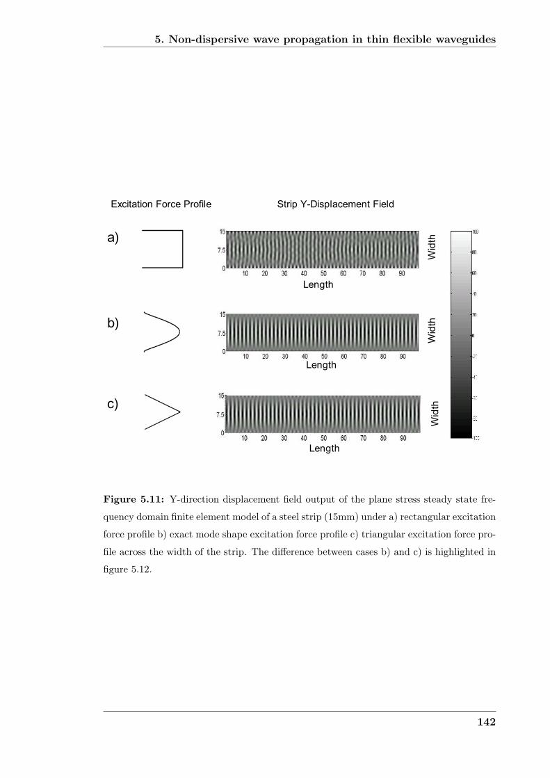
5. Non-dispersive wave propagation in thin flexible waveguides
� �
��������������� ������ ���������������� �����
��
��
�
��� ��
��� ��
��� ��
��� �
��� �
��� �
Figure 5.11: Y-direction displacement field output of the plane stress steady state fre-
quency domain finite element model of a steel strip (15mm) under a) rectangular excitation
force profile b) exact mode shape excitation force profile c) triangular excitation force pro-
file across the width of the strip. The difference between cases b) and c) is highlighted in
figure 5.12.
142
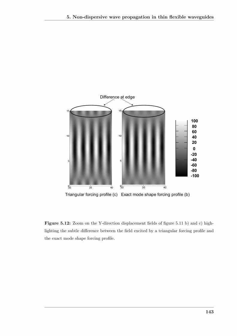
5. Non-dispersive wave propagation in thin flexible waveguides
� �
�
����
���
���
���
���
��
��
��
��
���
����������������������������� �������������������������������
��������������
Figure 5.12: Zoom on the Y-direction displacement fields of figure 5.11 b) and c) high-
lighting the subtle difference between the field excited by a triangular forcing profile and
the exact mode shape forcing profile.
143
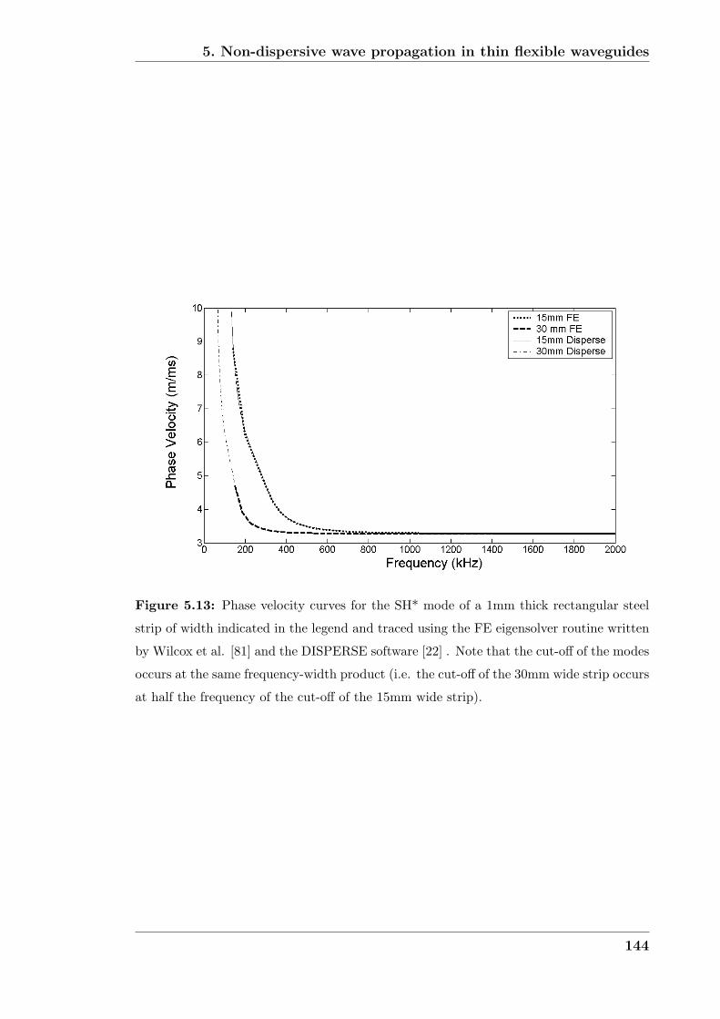
5. Non-dispersive wave propagation in thin flexible waveguides
Figure 5.13: Phase velocity curves for the SH* mode of a 1mm thick rectangular steel
strip of width indicated in the legend and traced using the FE eigensolver routine written
by Wilcox et al. [81] and the DISPERSE software [22] . Note that the cut-off of the modes
occurs at the same frequency-width product (i.e. the cut-off of the 30mm wide strip occurs
at half the frequency of the cut-off of the 15mm wide strip).
144
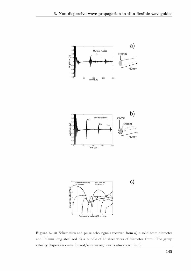
5. Non-dispersive wave propagation in thin flexible waveguides
� �
∅���
�����
����������� ���
� �
∅���
�����
∅���
����
������
���������� ���
��
� �
��
Figure 5.14: Schematics and pulse echo signals received from a) a solid 5mm diameter
and 160mm long steel rod b) a bundle of 18 steel wires of diameter 1mm. The group
velocity dispersion curve for rod/wire waveguides is also shown in c).
145
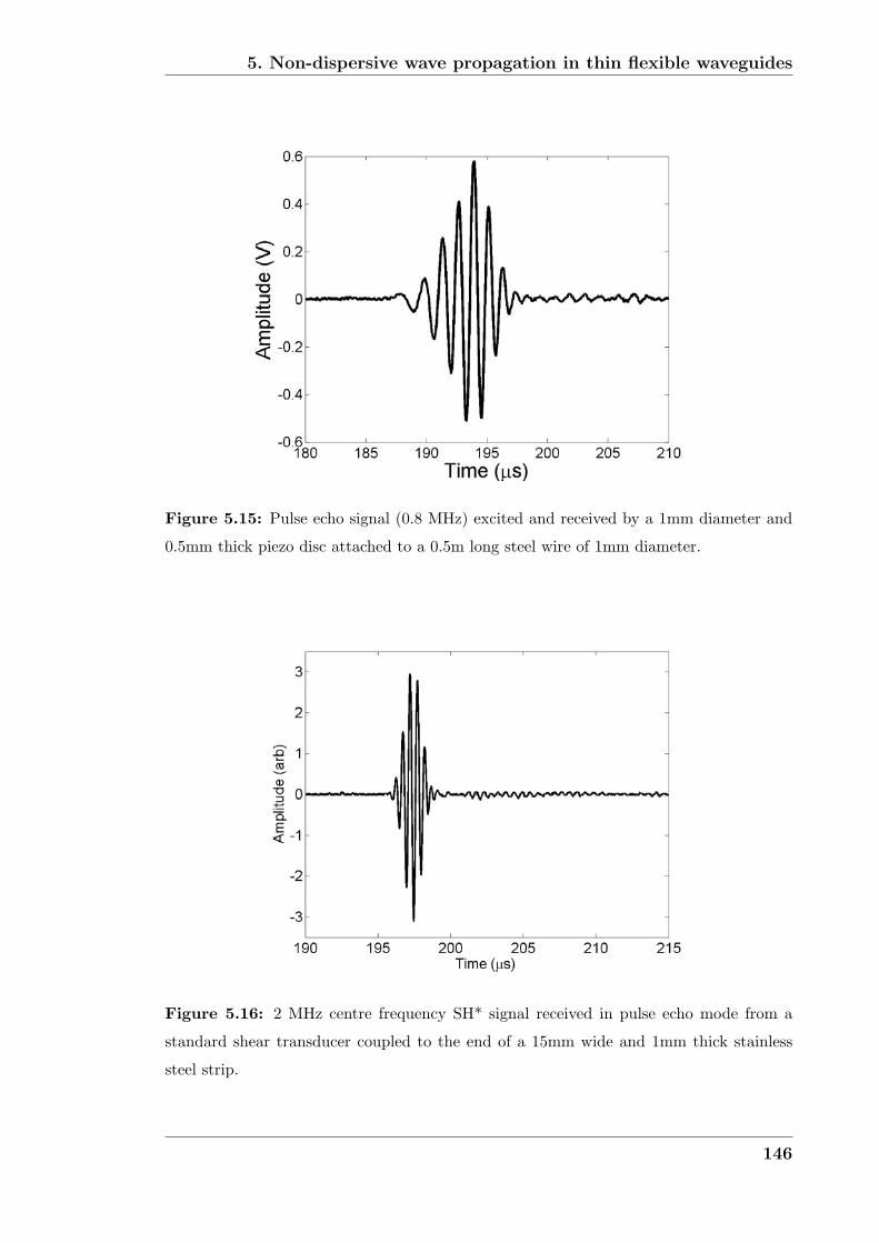
5. Non-dispersive wave propagation in thin flexible waveguides
Figure 5.15: Pulse echo signal (0.8 MHz) excited and received by a 1mm diameter and
0.5mm thick piezo disc attached to a 0.5m long steel wire of 1mm diameter.
Figure 5.16: 2 MHz centre frequency SH* signal received in pulse echo mode from a
standard shear transducer coupled to the end of a 15mm wide and 1mm thick stainless
steel strip.
146

5. Non-dispersive wave propagation in thin flexible waveguides
� �
�
��
��
Figure 5.17: a) Sketch of the in-plane laser doppler vibrometer scanning configuration
along the strip. b) Two dimensional fourier transform of in plane surface displacements
(polarised in the width direction of the strip) along the centre line of 1mm thick and 30mm
wide the steel strip. The dashed line (- - -) shows the predicted dispersion relation for the
SH* mode of steel (ρ = 7932kg/m3, Cl = 6000 m/s, Cs = 3060 m/s).
147

5. Non-dispersive wave propagation in thin flexible waveguides
Figure 5.18: 10 cycle 2 MHz centre frequency A0* signal received in pulse echo mode
from a standard shear transducer coupled to the end of a 30mm wide and 0.2mm thick
stainless steel strip.
148
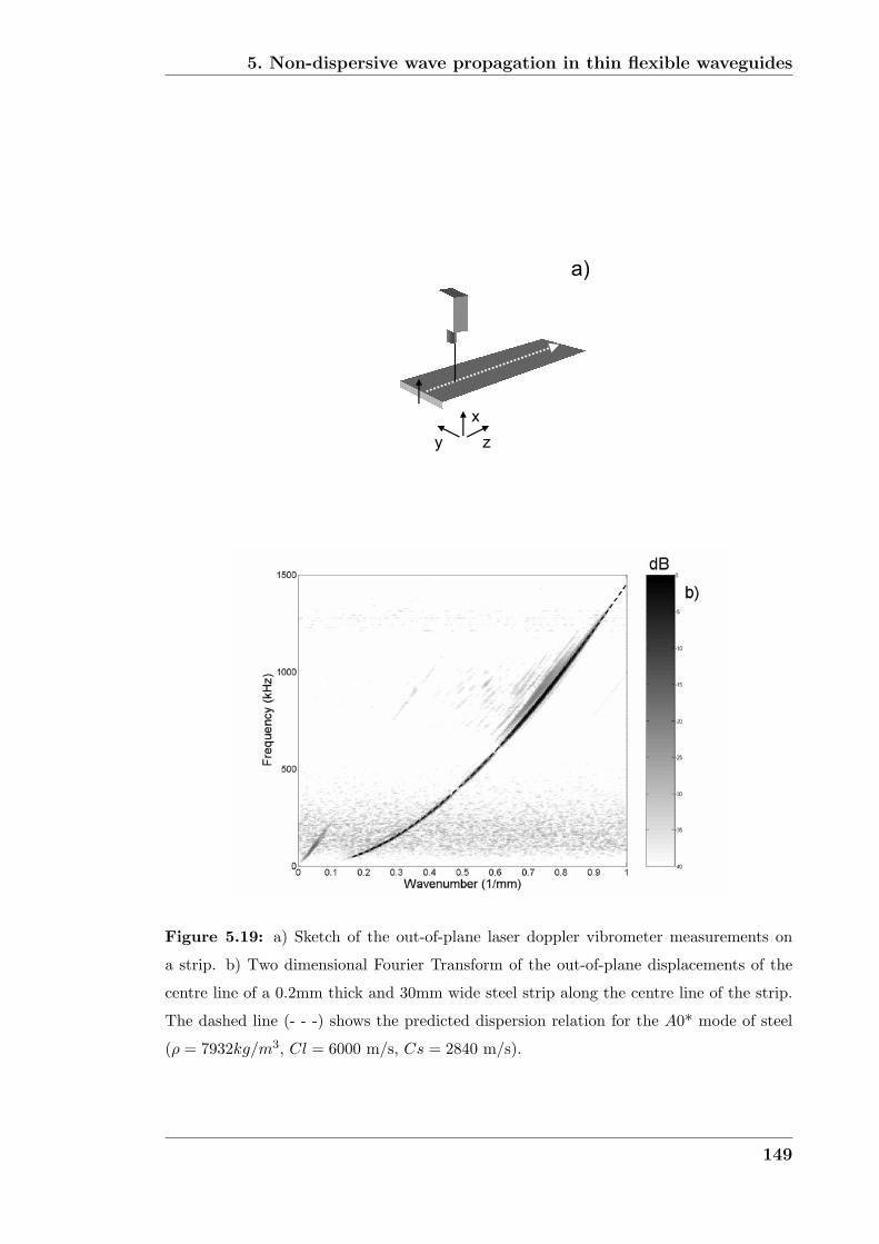
5. Non-dispersive wave propagation in thin flexible waveguides
� �
��
�
��
Figure 5.19: a) Sketch of the out-of-plane laser doppler vibrometer measurements on
a strip. b) Two dimensional Fourier Transform of the out-of-plane displacements of the
centre line of a 0.2mm thick and 30mm wide steel strip along the centre line of the strip.
The dashed line (- - -) shows the predicted dispersion relation for the A0* mode of steel
(ρ = 7932kg/m3, Cl = 6000 m/s, Cs = 2840 m/s).
149
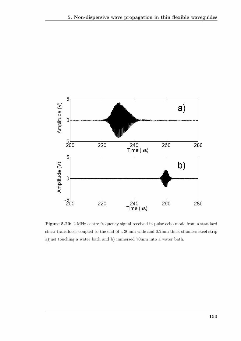
5. Non-dispersive wave propagation in thin flexible waveguides
Figure 5.20: 2 MHz centre frequency signal received in pulse echo mode from a standard
shear transducer coupled to the end of a 30mm wide and 0.2mm thick stainless steel strip
a)just touching a water bath and b) immersed 70mm into a water bath.
150
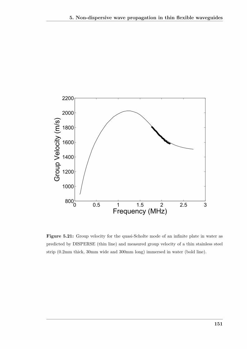
5. Non-dispersive wave propagation in thin flexible waveguides
0 0.5 1 1.5 2 2.5 3800
1000
1200
1400
1600
1800
2000
2200
Frequency (MHz)
Gro
up
Ve
locity (
m/s
)
Figure 5.21: Group velocity for the quasi-Scholte mode of an infinite plate in water as
predicted by DISPERSE (thin line) and measured group velocity of a thin stainless steel
strip (0.2mm thick, 30mm wide and 300mm long) immersed in water (bold line).
151

Chapter 6
Waveguide sources on half spaces
In the previous chapter wave propagation along thin flexible waveguides was dis-
cussed. The objective was to find a waveguide geometry that allowed the transmis-
sion of a strong and undistorted signal over relatively long distances. The traditional
approach of reducing the frequency thickness product of the waveguide and a new
approach using a single shear horizontal mode at higher frequencies were identified
as possible techniques.
Once the ultrasonic energy has been excited in the waveguide and a signal has been
transmitted non dispersively along the waveguide up to the surface of the object
that is to be interrogated, the ultrasonic signal has to enter the object. This is a
completely new challenge and the junction of the waveguide and the structure has to
be optimised to transmit a maximum of energy in the direction of interest within the
structure without distorting the signal. Therefore the characteristics of waveguide
sources on the structure has to be studied.
This chapter is dedicated to the investigation of waveguide source characteristics on
half spaces of elastic material. Semi-infinite half spaces are used since the waveg-
uide is believed to be thin and flexible, which implies that its thickness is small
compared to the structure and even the wavelength of the wave. Once attached to
the structure the waveguide will transmit stresses and displacements from its free
152

6. Waveguide sources on half spaces
end (transducer location) to the surface of the structure. It is assumed that the strip
has very low impedance compared to the half space and therefore does not restrain
the surface of the half space. This conveniently makes it possible to uncouple the
waveguide from the surface and simply consider a surface loaded by a distribution
of forces.
Traditionally the solution to surface loading of a half space has attracted a great
deal of interest and many publications can be found on this subject. However the
subject is complex and many lengthy mathematical elaborations can be found in
textbooks. Graff [17] and Achenbach [90] give excellent descriptions of the solution
methods for sources on half spaces. A detailed study of the techniques is far beyond
the scope of this chapter, therefore only the simplest solution for an anti-plane shear
line source will be outlined. For other cases the solutions that were reported in the
literature will be quoted and their significance with respect to the waveguide source
will be discussed.
6.1 Strip sources on a half space
Figure 6.1 displays schematics of the different loading conditions for strip sources
that were considered. The loads are constant across the strip so that in the limit of
infinitely small thickness a perfect line source is obtained. The infinite strip source
in this case represents a plate mode entering the half space from an infinitely wide
plate. The mode amplitude is uniform across the width. Even though in real life
the waveguide will be a finite strip and the mode amplitude will not necessarily be
uniform across the width of the strip the line source is a good approximation because
the aspect ratio of the strip is large and while the thickness will be of the order of
a wavelength the strip will be many wavelengths wide. The different fundamental
modes in a plate represent the various loading cases. The S0 mode will cause normal
loading of the half space, the SH0 mode will cause anti-plane shear loading and the
A0 mode will cause tangential shear loading. The S0 and SH0 modes are the most
interesting since they can propagate with low dispersion in the waveguide leading
to the source point on the half space.
153
6. Waveguide sources on half spaces
The solution for normal or tangential in-plane loading of a strip source on a half
space is much more complicated than anti-plane shear loading. Due to normal and
tangential in-plane sources, a shear, a compressional and a Rayleigh surface wave
are excited in the half space in order to satisfy the boundary condition imposed by
the loads. The problem is also commonly known as ’Lamb’s problem’ since Lamb
[91] was the first to present a solution. Graff [17] gives references to researchers who
subsequently contributed to or extended the analysis.
The work by Miller and Pursey [92] is one of the most comprehensive and it is often
quoted in the context of waves excited by surface loads. The expressions that they
derived for the distribution of shear and compressional waves excited by different
surface sources will be recalled. Surface waves will also be excited by the sources.
However surface waves do not penetrate into the structure and thus become of
limited use for structural investigations. Therefore this study was focused on the
shear and compressional waves that spread into the half space. The case of tangential
anti-plane shear loading of the half space will be considered first.
6.1.1 Tangential anti-plane loading
The analysis presented here follows that presented by Graff [17] and Achenbach [90]
closely. Consider the half space displayed in figure 6.1a. The half space is defined
by y ≥ 0. Waves are generated by a distribution of harmonically oscillating loads
represented by
σyz(x, 0, z, t) = τ(x)eiωt (6.1)
σyy(x, 0, z, t) = σyx(x, 0, z, t) = 0. (6.2)
The problem is uniform in the z-direction and therefore two dimensional. The shear
tractions cause motion in the z direction only (uz = uz(x, y, t)), and the equations
154

6. Waveguide sources on half spaces
of motion can be reduced to
∂2uz
∂x2+
∂2uz
∂y2=
1
C2T
∂2uz
∂t2(6.3)
where CT is the shear wave velocity in the half space. By assuming harmonically
oscillating displacements of the form
uz(x, y, t) = uz(x, y)eiωt (6.4)
and the identity kT = ωCT
equation 6.3 reduces to
∂2uz
∂x2+
∂2uz
∂y2+ k2
T uz = 0. (6.5)
The boundary condition due to the surface load can now also be expressed as
μ∂uz
∂y= τ(x) at y=0 (6.6)
where μ is the shear modulus of the material. Using Fourier transformation (indi-
cated by adding * to a variable) equation 6.5 can be rewritten in the form of an
ordinary partial differential equation
∂2u∗z
∂y2− (ξ2 − k2
T )u∗z = 0. (6.7)
with solution
u ∗z (ξ, y, ω) = Ae−γy + Beγy (6.8)
where
γ2 = ξ2 − k2T . (6.9)
155
6. Waveguide sources on half spaces
Using the transformed boundary condition from 6.6
μ∂u∗z
∂y= τ ∗ (ξ) at y=0. (6.10)
results in the solution in the Fourier domain
u ∗z (ξ, y) = −τ(ξ)
μγe−γy. (6.11)
All that remains is to invert the solution
uz(x, y) = − 1
μ2π
∫ ∞
−∞
τ ∗ (ξ)
γe−γye−iξxdξ. (6.12)
and insert the specific loading conditions in the integral. For a strip of uniformly
applied loads as shown in figure 6.1a this is expressed by
τ(x) =
⎧⎨⎩ τ0, for | x |< a
0, for | x |> a(6.13)
and in Fourier transformed form
τ ∗ (ξ) =2τ0
2π
sinξa
ξa. (6.14)
therefore the solution for the anti-plane strip loading becomes
uz(x, y) = − τ0
μπ
∫ ∞
−∞
sinξa
γξae−γye−iξxdξ. (6.15)
Equation 6.15 is the solution to the problem. However equation 6.15 is in form of
an integral. The evaluation of this integral is usually the most challenging part of
the analysis. Achenbach [90] shows a lengthy derivation for the special case of a line
source, when the strip width ’2a’ tends to zero. The solution is transformed into
polar coordinates and the final result becomes
uz(x, y, ω) =Pi
2μH
(2)0 (kT r) (6.16)
156
6. Waveguide sources on half spaces
where r is the distance from the origin located at x = y = 0, P is the loading force,
μ the shear modulus of the material and H20 (x) is the Hankel function of the second
kind.
Equation 6.16 shows that the displacement field is entirely dependent on the distance
(radius) of a point in the half space from the source point, the field therefore spreads
cylindrically into the half space. Figure 6.2 shows a contour plot of the magnitude
of the displacement field computed using equation 6.16 for a SH line source on a
half space.
6.1.2 Normal line source loading
Miller and Pursey [92] found an approximation for the displacements in the field
far from a very thin strip source of thickness 2a. They separated the displacement
fields into displacements due to compressional waves (UR) and displacements due to
shear waves (Uθ)
uR ∼ aei(3/4π−R)
μ
√2
πR
cosθ(k2 − 2sin2θ)
F0(sinθ)(6.17)
uθ ∼ aei(5/4π−kR)
μ
√2k5
πR
sin2θ√
k2sin2θ − 1
F0(ksinθ)(6.18)
where
F0(ξ) = (2ξ2 − k2)2 − 4ξ2(ξ2 − 1)1/2(ξ2 − k2)1/2 (6.19)
and
k2 =C2
l
C2s
. (6.20)
In the above equation R is the distance (radius) from the origin (centre of the
strip), θ is the angle from the normal (y direction) and μ is the shear modulus
of the material. The normalised result of these functions for a steel half space is
157
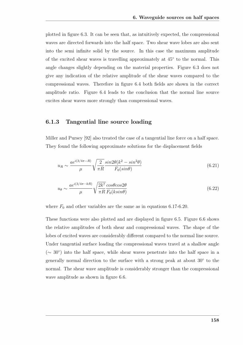
6. Waveguide sources on half spaces
plotted in figure 6.3. It can be seen that, as intuitively expected, the compressional
waves are directed forwards into the half space. Two shear wave lobes are also sent
into the semi infinite solid by the source. In this case the maximum amplitude
of the excited shear waves is travelling approximately at 45◦ to the normal. This
angle changes slightly depending on the material properties. Figure 6.3 does not
give any indication of the relative amplitude of the shear waves compared to the
compressional waves. Therefore in figure 6.4 both fields are shown in the correct
amplitude ratio. Figure 6.4 leads to the conclusion that the normal line source
excites shear waves more strongly than compressional waves.
6.1.3 Tangential line source loading
Miller and Pursey [92] also treated the case of a tangential line force on a half space.
They found the following approximate solutions for the displacement fields
uR ∼ aei(3/4π−R)
μ
√2
πR
sin2θ(k2 − sin2θ)
F0(sinθ)(6.21)
uθ ∼ aei(3/4π−kR)
μ
√2k7
πR
cosθcos2θ
F0(ksinθ)(6.22)
where F0 and other variables are the same as in equations 6.17-6.20.
These functions were also plotted and are displayed in figure 6.5. Figure 6.6 shows
the relative amplitudes of both shear and compressional waves. The shape of the
lobes of excited waves are considerably different compared to the normal line source.
Under tangential surface loading the compressional waves travel at a shallow angle
(∼ 30◦) into the half space, while shear waves penetrate into the half space in a
generally normal direction to the surface with a strong peak at about 30◦ to the
normal. The shear wave amplitude is considerably stronger than the compressional
wave amplitude as shown in figure 6.6.
158
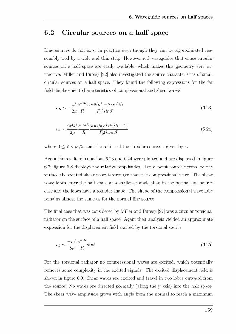
6. Waveguide sources on half spaces
6.2 Circular sources on a half space
Line sources do not exist in practice even though they can be approximated rea-
sonably well by a wide and thin strip. However rod waveguides that cause circular
sources on a half space are easily available, which makes this geometry very at-
tractive. Miller and Pursey [92] also investigated the source characteristics of small
circular sources on a half space. They found the following expressions for the far
field displacement characteristics of compressional and shear waves:
uR ∼ − a2
2μ
e−iR
R
cosθ(k2 − 2sin2θ)
F0(sinθ)(6.23)
uθ ∼ ia2k3
2μ
e−ikR
R
sin2θ(k2sin2θ − 1)
F0(ksinθ)(6.24)
where 0 ≤ θ < pi/2, and the radius of the circular source is given by a.
Again the results of equations 6.23 and 6.24 were plotted and are displayed in figure
6.7; figure 6.8 displays the relative amplitudes. For a point source normal to the
surface the excited shear wave is stronger than the compressional wave. The shear
wave lobes enter the half space at a shallower angle than in the normal line source
case and the lobes have a rounder shape. The shape of the compressional wave lobe
remains almost the same as for the normal line source.
The final case that was considered by Miller and Pursey [92] was a circular torsional
radiator on the surface of a half space. Again their analysis yielded an approximate
expression for the displacement field excited by the torsional source
uθ ∼ −ia4
8μ
e−iR
Rsinθ (6.25)
For the torsional radiator no compressional waves are excited, which potentially
removes some complexity in the excited signals. The excited displacement field is
shown in figure 6.9. Shear waves are excited and travel in two lobes outward from
the source. No waves are directed normally (along the y axis) into the half space.
The shear wave amplitude grows with angle from the normal to reach a maximum
159
6. Waveguide sources on half spaces
when the waves are travelling parallel to the surface.
In a second paper Miller and Pursey [93] investigated how much of the source en-
ergy from a normal point source is converted into each of the different wave types.
Woods [94] summarised this information in the sketch shown in figure 6.10. Most
of the source energy is transformed into a Rayleigh wave and stays trapped at the
surface. Only 26% of the energy converts into shear waves that travel at an angle
∼ 45◦ to the excitation (y) direction. Just 7% of the energy is converted into com-
pressional waves that travel normal to the surface into the material (in the direction
of the source and y axis). A normal point source is very efficient at creating surface
disturbances but rather bad at exciting waves that penetrate into the material.
Miller and Pursey [93] further investigated the effect of the energy transfer of a
combination of sources on the surface. They found that by augmenting the number
of sources to three and distributing them in an equilateral triangle the amount of
energy that is transferred into compressional waves (∼ 31%) can be increased to
come close to that of the shear wave energy (∼ 43%) and even exceed the energy
converted into a surface wave (∼ 26%). But such sources become more complicated
to create and if each of them were separate waveguides the interpretation of results
would be complicated by crosstalk.
6.3 Choice of the most suitable waveguide source
on a half space
In chapter 5 it was shown that several strategies can be successfully employed to
achieve non-dispersive wave propagation along a waveguide. The geometry of the
waveguide dictates which type of wave mode (shear/compressional/flexural) can
successfully be excited and propagate non-dispersively in a certain range of frequen-
cies. However the waveguide geometry also determines the source geometry unless
the system is even further complicated by creating an adapter section that con-
nects the waveguide to the object surface. The radiation patterns of bulk shear and
160
6. Waveguide sources on half spaces
compressional waves due to line sources, strip sources and circular point sources
show that for cases with normal loading, i.e. compressional waves incident from the
waveguide, a dominating surface wave and strong shear waves at about ∼ 45◦ to
the normal are excited. The fraction of energy excited as compressional waves is
very low, ∼ 7% for a circular point source. The geometry change from a circular
point source to a line source does not show a great deal of improvement. Therefore
a waveguide that transmits and receives compressional waves is not very efficient for
thickness gauging of a structure from a remote location.
Circular torsional radiators on a half space show improvements compared to the
normally loading sources since only shear waves are excited in the object. However
the polar distribution of the excited shear waves is not ideal. Surface skimming
shear waves are excited most strongly, while no waves at all are excited in the di-
rection normal to the surface (y axis). Another problem is the reception quality of
such torsional radiators. A shear wave that will be scattered back to the source area
(junction of waveguide and object), will not be polarised to excite torsional waves
in the waveguide. The polarisation of such waves would be more optimised to excite
flexural waves, however these would not be effectively received by a torsional wave
transducer at the end of the waveguide.
Line sources that cause normal tangential loading on a half-space show favorable
source characteristics compared to normal line sources. Shear waves are excited
strongly in a direction parallel to the waveguide axis. However surface waves and
compressional waves at non-normal angles are also excited. This method was also
ruled out because it would need a strongly dispersive flexural waveguide mode to
act as a source. This would complicate the design of the excitation method.
It was found that a line or strip source exciting anti-plane shear motion showed the
most desirable source characteristics. An anti-plane shear source solely excites shear
horizontal waves in the half space. Surface waves or compressional waves are not
excited. Also an ideal line source causes perfectly cylindrical spreading of wavefronts
in the half space. This ensures that all areas of the half space are irradiated equally
161
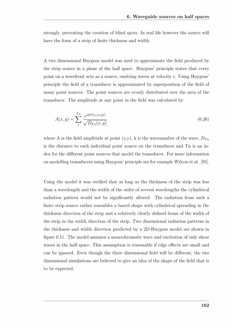
6. Waveguide sources on half spaces
strongly, preventing the creation of blind spots. In real life however the source will
have the form of a strip of finite thickness and width.
A two dimensional Huygens model was used to approximate the field produced by
the strip source in a plane of the half space. Huygens’ principle states that every
point on a wavefront acts as a source, emitting waves at velocity c. Using Huygens’
principle the field of a transducer is approximated by superposition of the field of
many point sources. The point sources are evenly distributed over the area of the
transducer. The amplitude at any point in the field was calculated by:
A(x, y) =Tn∑1
e(ikDTn(x,y))√DTn(x, y)
(6.26)
where A is the field amplitude at point (x,y), k is the wavenumber of the wave, DTn
is the distance to each individual point source on the transducer and Tn is an in-
dex for the different point sources that model the transducer. For more information
on modelling transducers using Huygens’ principle see for example Wilcox et al. [95].
Using the model it was verified that as long as the thickness of the strip was less
than a wavelength and the width of the order of several wavelengths the cylindrical
radiation pattern would not be significantly altered. The radiation from such a
finite strip source rather resembles a barrel shape with cylindrical spreading in the
thickness direction of the strip and a relatively clearly defined beam of the width of
the strip in the width direction of the strip. Two dimensional radiation patterns in
the thickness and width direction predicted by a 2D-Huygens model are shown in
figure 6.11. The model assumes a monochromatic wave and excitation of only shear
waves in the half space. This assumption is reasonable if edge effects are small and
can be ignored. Even though the three dimensional field will be different, the two
dimensional simulations are believed to give an idea of the shape of the field that is
to be expected.
162

6. Waveguide sources on half spaces
6.4 Wave reflection at the waveguide half space
joint
The ideal configuration of the ’acoustic cable’ allows it to be operated in pulse
echo mode. Here a signal is sent along the waveguide, transforms into a bulk wave
in the structure, interacts with features of the structure, returns to the waveg-
uide/structure junction and is converted into the same waveguide mode to be finally
picked up by the transducer again. Therefore it is necessary for the waveguide source
to efficiently excite waves in the right direction. It also has to be ensured that most
of the energy enters the structure, otherwise a very large entry reflection might mask
the more interesting signals that return from the object to be investigated.
A finite element study was carried out to investigate the influence of the strip thick-
ness on the size of the entry reflection. A three dimensional model of thin steel
(ρ = 7932kg/m3, Cl = 6000m/s and Cs = 3260m/s) strips entering an infinite plate
at normal angle was created. The plate was 6mm thick and the infinite direction
was modelled by 3mm of real elements connected to infinite elements at the edges
in order to extend the boundary to infinity. These infinite elements were also used
at the edge of the strip and the block to extend the width of both to infinity. (The
reader may rightly wonder why the model was not carried out in two dimensions if
the width of the strip was made infinite; however a three dimensional model had to
be used because the ABAQUS explicit finite element software does not model shear
horizontal waves in two dimensions). A symmetry condition in the centre of the
strip was used to reduce the model size. The mesh was made up of cubic elements
of sizes between 1/8 − 1/10 of the shear wavelength of the material at the centre
frequency. Sketches of the side view, top view as well as a three dimensional view of
the model are shown in figure 6.12. The mesh and the infinite element boundaries
that were used for the analysis are also shown in the figure.
The ABAQUS finite element software was used. A time marching explicit solver
that automatically determines the time step was chosen and a uniform anti-plane
shear load was applied across the strips end section. Temporally a 5 cycle Hanning
163
6. Waveguide sources on half spaces
windowed toneburst at 2 MHz centre frequency was applied. Signals were monitored
at a point in the centre of the strip at the excitation location, see figure 6.12. The
analysis resulted in time traces such as the one shown in figure 6.13.
The reflection coefficient was determined from the results for strips of thicknesses
0.25− 1.5mm. The incoming signal was isolated and the entry reflection signal was
isolated. The Fourier transforms of both signals were obtained and the reflection
coefficient was defined as ratio of the amplitude of the signal reflected by the junction
and the incoming signal at the centre frequency (2MHz)
CEntry =Areflected
Aincoming
. (6.27)
Figure 6.14 shows the reflection coefficients obtained for different thicknesses of
strips. The figure clearly shows that the thinner the strip is the more energy is
reflected. (This result is in agreement with results reported by Vogt [36] for the
entry reflection of the L(0, 1) mode of a thin wire embedded in curing adhesives
like epoxy.) The thicker the strip becomes the more energy is transferred into the
half-space and the more collimated its beam becomes. Once the thickness of the
source exceeds a bulk wavelength in the material side lobes will appear in the field
excited by the source; this is believed to be undesirable since it limits the field of
view. For the current operational frequency of 2 MHz the shear wavelength of steel
is approximately 1.5mm. Therefore a waveguide strip of thickness of about 1mm
will still show good performance without any local minima (blind spots in the field
of view) in the beam pattern .
6.5 Summary
In this chapter the source characteristics of different waveguide sources on a half
space were considered. The waveguide was considered to transmit a distribution
of loads to the surface of the object, which is modelled as a half space since it is
assumed to be much larger than the thin and flexible waveguide. This allowed the
analysis of the strip and object to be uncoupled so that the forcing from the strip
164
6. Waveguide sources on half spaces
was simply modelled as distribution of loads on a half space. The subject has been
thoroughly treated in the literature. Work presented in text books such as Graff
[17] and excellent papers on different sources on infinite elastic solids by Miller and
Pursey [92], [93] was recalled and its consequences for the purpose of remote waveg-
uide excitation and reception were considered.
It was found that a source of anti-plane shear on a half space was most suited to the
application. Other sources, especially those with normal loading, have the disad-
vantage of sending a very strong surface wave, a strong shear wave and a very weak
compressional wave at different angles into the structure. For torsional sources the
excitation of shear waves alone is possible, however reception would have to occur
in the form of flexural modes which are not well suited for transmission along the
waveguide. For the same reason tangential shear sources on the half space were
ruled out.
The selected anti-plane shear source had the advantage of only exciting shear hori-
zontal waves in the half space. The waves also spread cylindrically into the object
under investigation which maximises the field of view. The entry reflection is min-
imised when the strip thickness is large, however in order to ensure reasonably
cylindrical spreading of the wave in the half space the waveguide thickness has to
stay below the wavelength of a shear bulk wave.
165
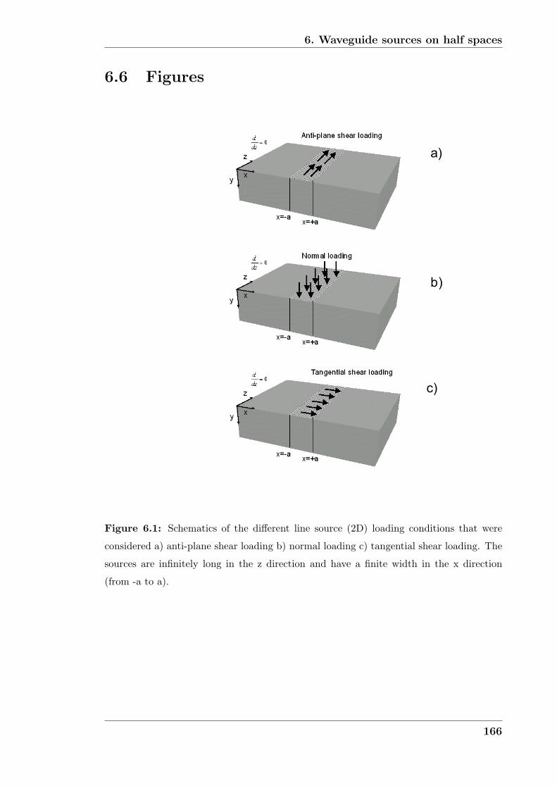
6. Waveguide sources on half spaces
6.6 Figures
��
��
��
Figure 6.1: Schematics of the different line source (2D) loading conditions that were
considered a) anti-plane shear loading b) normal loading c) tangential shear loading. The
sources are infinitely long in the z direction and have a finite width in the x direction
(from -a to a).
166
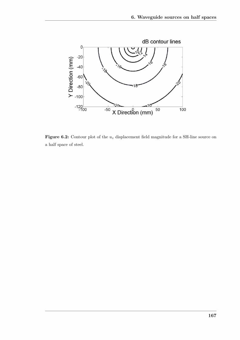
6. Waveguide sources on half spaces
Figure 6.2: Contour plot of the uz displacement field magnitude for a SH-line source on
a half space of steel.
167
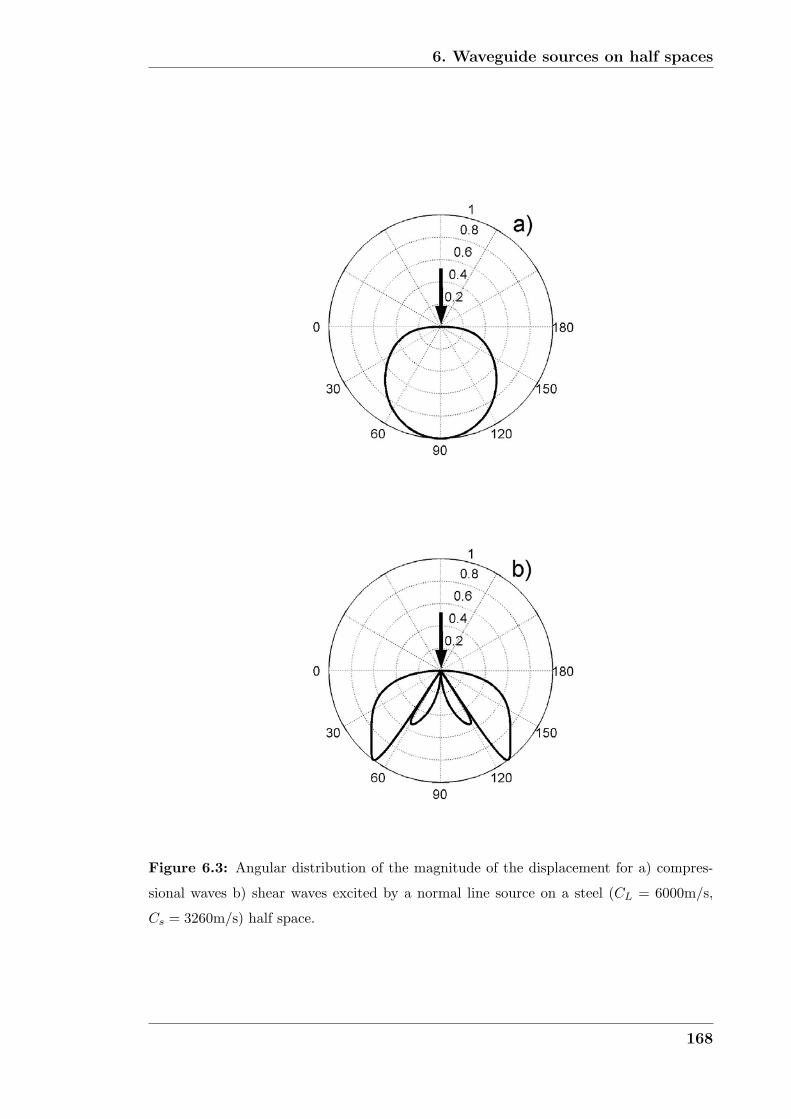
6. Waveguide sources on half spaces
Figure 6.3: Angular distribution of the magnitude of the displacement for a) compres-
sional waves b) shear waves excited by a normal line source on a steel (CL = 6000m/s,
Cs = 3260m/s) half space.
168
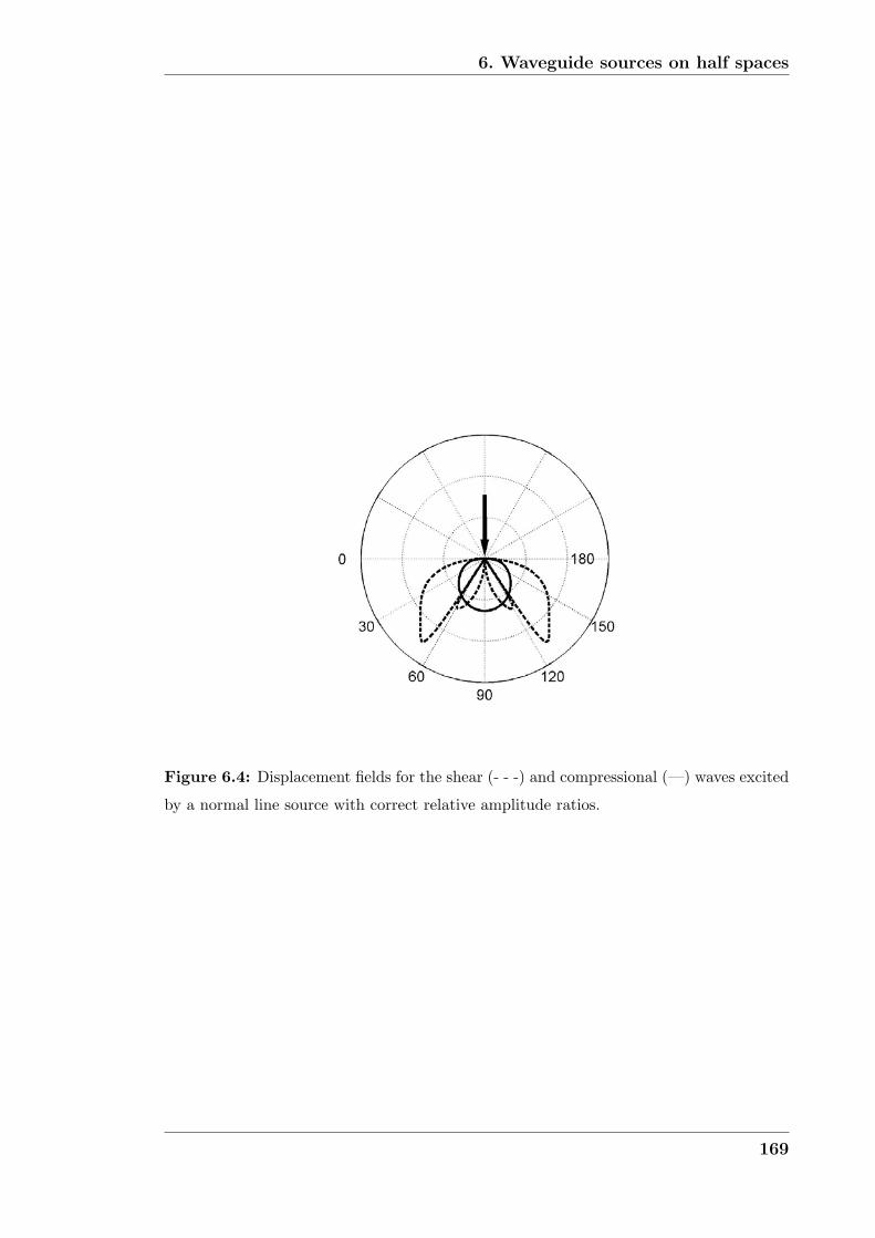
6. Waveguide sources on half spaces
Figure 6.4: Displacement fields for the shear (- - -) and compressional (—) waves excited
by a normal line source with correct relative amplitude ratios.
169

6. Waveguide sources on half spaces
Figure 6.5: Angular distribution of the magnitude of the displacement for a) com-
pressional waves b) shear waves excited by a tangential shear line source on a steel
(CL = 6000m/s, Cs = 3260m/s) half space.
170

6. Waveguide sources on half spaces
Figure 6.6: Displacement fields for the shear (- - -) and compressional (—) waves excited
by a tangential shear line source with correct relative amplitude ratios.
171
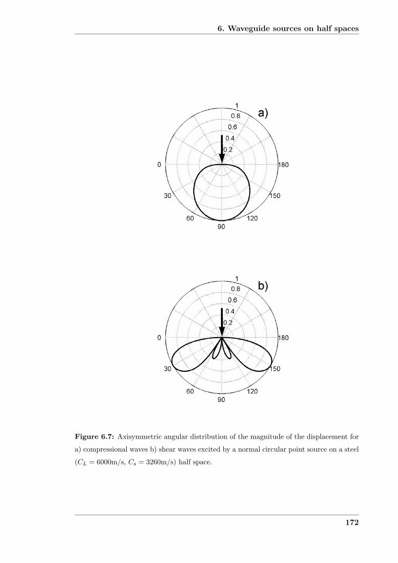
6. Waveguide sources on half spaces
Figure 6.7: Axisymmetric angular distribution of the magnitude of the displacement for
a) compressional waves b) shear waves excited by a normal circular point source on a steel
(CL = 6000m/s, Cs = 3260m/s) half space.
172
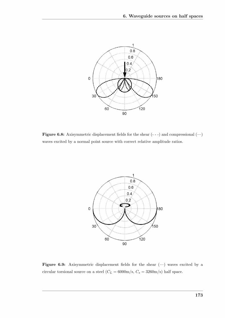
6. Waveguide sources on half spaces
Figure 6.8: Axisymmetric displacement fields for the shear (- - -) and compressional (—)
waves excited by a normal point source with correct relative amplitude ratios.
Figure 6.9: Axisymmetric displacement fields for the shear (—) waves excited by a
circular torsional source on a steel (CL = 6000m/s, Cs = 3260m/s) half space.
173

6. Waveguide sources on half spaces
����� ��� ������� ��������� �
������ ���
� � ��
� �
������� ����������� �
������ ����� ���
�������� �#
$��% ������ #�
Figure 6.10: Sketch of the different wave types excited by a normal point force on a half
space and their share of the total excitation energy. (After Woods [94] , for Poisson’s ratio
∼ 1/4)
174

6. Waveguide sources on half spaces
x
plan view
Thickness
Width
Half space
depth
Thic
kness d
irection (
mm
)
Half space depth (mm)
dB
0
- 5
- 10
- 15
- 20
- 25
0
- 5
- 10
- 15
- 20
- 25
- 30
Wid
th d
irection (
mm
)
Half space depth (mm)
dB
a)
b)
Figure 6.11: Two dimensional Huygens models of a) a 1mm source and b) a 15mm
source in a plane. The sources are modelled by 21 point sources distributed evenly along
the transducer line. The wavelength is 1.5mm which approximately corresponds to a
2MHz shear wave in steel.
175

6. Waveguide sources on half spaces
��������������
���������������
�������������������������
�����
���
��
�����
������
�����
�
���
���
���������
����������������
����������������
�
����� �����
���
������
�����������������
������
����
����
� ��� ������ ���
��������
�����������������������������
� ������!�
������
��������������
����������������������
�����
�����
Figure 6.12: Schematic of the finite element mesh used to analyse the reflection coefficient
of a shear horizontal wave in a waveguide entering a half space of the same material (steel).
176
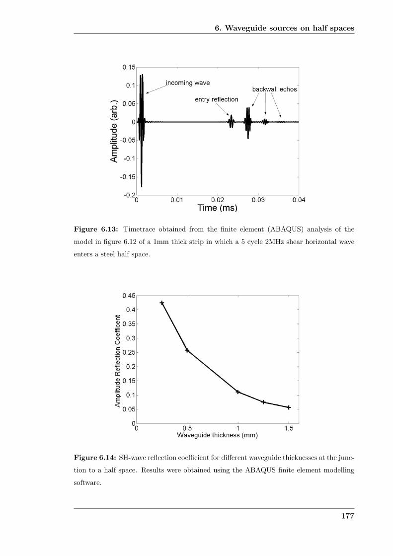
6. Waveguide sources on half spaces
Figure 6.13: Timetrace obtained from the finite element (ABAQUS) analysis of the
model in figure 6.12 of a 1mm thick strip in which a 5 cycle 2MHz shear horizontal wave
enters a steel half space.
Figure 6.14: SH-wave reflection coefficient for different waveguide thicknesses at the junc-
tion to a half space. Results were obtained using the ABAQUS finite element modelling
software.
177

Chapter 7
Remote thickness gauging using a
waveguide
7.1 The waveguide-structure joint
The outcome of chapter 6 showed that theoretically a shear horizontal line source
is best suited for exciting waves in an object that is to be investigated. Simulations
showed that a perfect joint between the waveguide and a plate of the same material
ensured that most of the energy was transmitted from the waveguide into the object
(see section 6.4).
In practice the position of attachment of the waveguide is rarely known prior to the
installation of the structure; the waveguide is added later for monitoring applica-
tions. Therefore the waveguide will have to be attached to the structure in some
way. Permanent attachment is possible by bonding, welding, brazing, soldering or
other methods. Detachable attachment methods like clamping can also be envis-
aged. The permanent attachment methods are potentially preferable because they
optimise ultrasonic coupling between both parts while clamped contact will cause
high losses even if a coupling agent is used. However defects in the bonding method
and alterations that it causes to the joint geometry might adversely affect the wave
propagation through the junction. Also the use of standard coupling agents will not
178
7. Remote thickness gauging using a waveguide
be possible at elevated temperatures. The different joining techniques were investi-
gated experimentally.
7.2 Experimental setups for thickness gauging
It was decided to set up a thickness gauging experiment to test the different joining
methods on specimens of the same thickness. The stainless steel strip geometry
(1mm thick, 15mm wide and 300mm long) and thickness of the steel plate specimen
(6mm) were kept constant while only the joining method was altered. The experi-
ments were carried out in the pulse echo and pitch catch modes. Measurements in
the pulse echo mode would be the preferred embodiment since only one waveguide
is needed to send and receive the signal. Figure 7.1 illustrates the different test
configurations.
Excitation of the SH* mode in the stainless steel strip was achieved in the same way
as in chapter 5. A 5 cycle 2MHz Hanning windowed toneburst was sent and received
by a standard ultrasonic shear transducer (Panametrics). The 13mm diameter shear
transducer was clamped to the waveguide end with treacle as a shear couplant. It
was ensured that the polarisation direction of the transducer was parallel to the
width of the strip. The clamp design was optimised to minimise its effect on the
mode propagating in the strip. The SH* mode energy is concentrated at the centre
of the strip (see section 5.4.1) and it is therefore not strongly influenced by attach-
ments to the edges. This arrangement was used to attach two blocks to either side
of the strip. The blocks sandwiched the edges of the strip and bolts were used to
tightly push the blocks onto the strip in order to strongly grip onto the edges of the
strip. A back plate was then bolted to the four blocks that were just clamped to
the strip. In between the back plate and the strip end a transducer was inserted
and thus clamped against the end of the strip. Figure 7.2 illustrates the transducer
clamp.
179
7. Remote thickness gauging using a waveguide
7.2.1 Coupling with coupling agent
The pulse echo mode experiment with treacle as coupling agent is the simplest: once
the surface of the plate had been evenly covered with treacle the strip was manually
pushed onto the surface at right angles. Signals were collected and are displayed in
figure 7.3.
Figure 7.3 shows a pulse echo signal when the strip is not in contact with the plate
and a signal when strip and plate are in contact. The signal when both pieces are
coupled is slightly less strong. However there are no additional echoes from within
the plate specimen, which leads to the conclusion that not enough energy is sent and
received through the shear-couplant joint to enable inspection of the plate specimen
in the pulse echo mode.
After the negative results of the pulse echo mode experiments, experiments in the
pitch catch mode (see figure 7.1 II a) were performed. Two strip waveguides were
fixed together so that they were roughly parallel and separated by a gap of 1mm
at the remote end with respect to the transducer. The assembly was then manu-
ally put in contact with the plate specimen. A signal was sent from one waveguide
and received on the other strip. Signals were collected and are displayed in figure 7.4.
For the pitch catch mode good results were obtained as shown in figure 7.4. The
signals are much weaker (∼ 30dB) than the control signal (unattached pulse echo
signal of the sending strip), however the backwall echoes from the plate specimen
are clearly visible. The better but weaker signals are achieved because only the
signals that were transmitted from the sending waveguide into the plate are picked
up by the receiving waveguide. In the pulse echo mode these weaker signals were
completely masked by coherent noise from waveguide modes that were either excited
by the transducer or caused by mode conversion at the junction of the strip and the
plate.
180
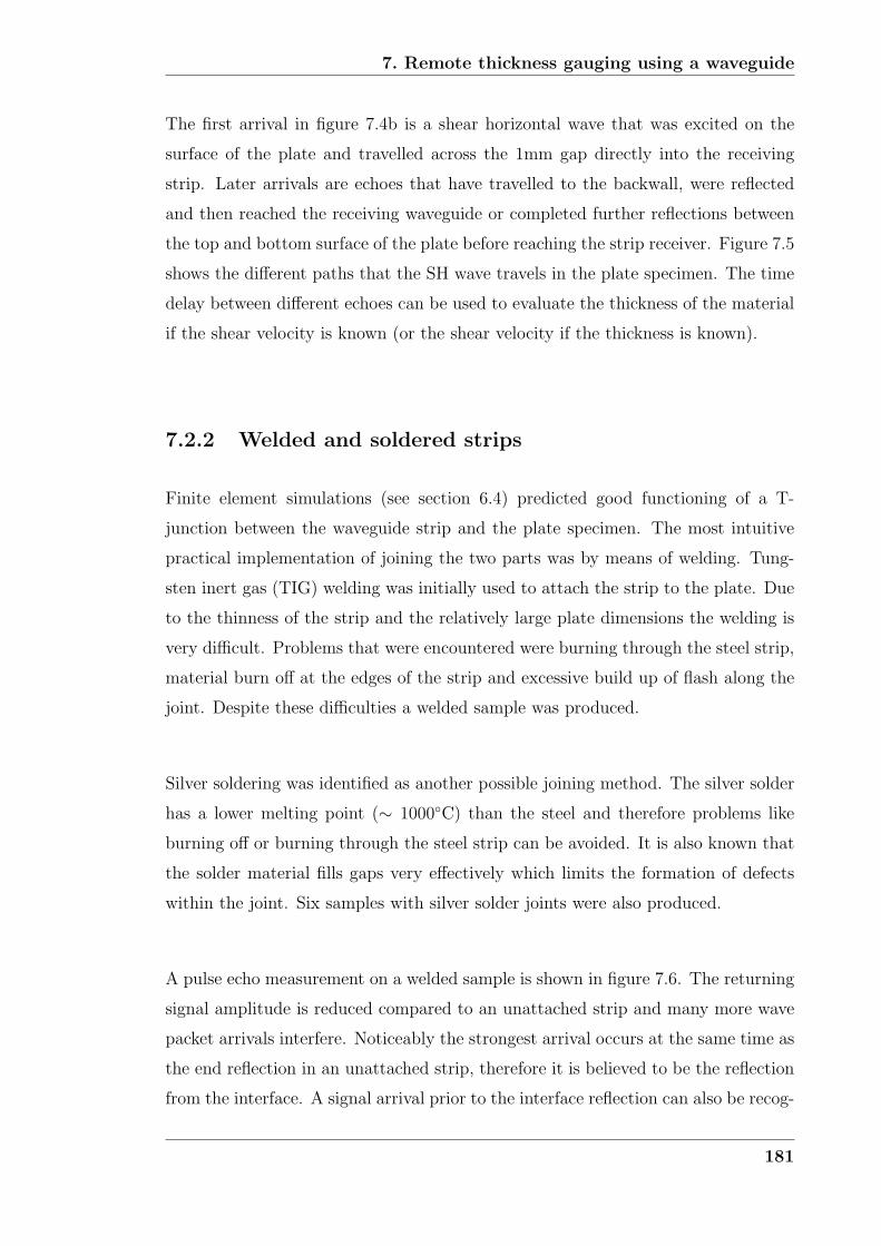
7. Remote thickness gauging using a waveguide
The first arrival in figure 7.4b is a shear horizontal wave that was excited on the
surface of the plate and travelled across the 1mm gap directly into the receiving
strip. Later arrivals are echoes that have travelled to the backwall, were reflected
and then reached the receiving waveguide or completed further reflections between
the top and bottom surface of the plate before reaching the strip receiver. Figure 7.5
shows the different paths that the SH wave travels in the plate specimen. The time
delay between different echoes can be used to evaluate the thickness of the material
if the shear velocity is known (or the shear velocity if the thickness is known).
7.2.2 Welded and soldered strips
Finite element simulations (see section 6.4) predicted good functioning of a T-
junction between the waveguide strip and the plate specimen. The most intuitive
practical implementation of joining the two parts was by means of welding. Tung-
sten inert gas (TIG) welding was initially used to attach the strip to the plate. Due
to the thinness of the strip and the relatively large plate dimensions the welding is
very difficult. Problems that were encountered were burning through the steel strip,
material burn off at the edges of the strip and excessive build up of flash along the
joint. Despite these difficulties a welded sample was produced.
Silver soldering was identified as another possible joining method. The silver solder
has a lower melting point (∼ 1000◦C) than the steel and therefore problems like
burning off or burning through the steel strip can be avoided. It is also known that
the solder material fills gaps very effectively which limits the formation of defects
within the joint. Six samples with silver solder joints were also produced.
A pulse echo measurement on a welded sample is shown in figure 7.6. The returning
signal amplitude is reduced compared to an unattached strip and many more wave
packet arrivals interfere. Noticeably the strongest arrival occurs at the same time as
the end reflection in an unattached strip, therefore it is believed to be the reflection
from the interface. A signal arrival prior to the interface reflection can also be recog-
181

7. Remote thickness gauging using a waveguide
nised. This signal is believed to be due to flash and defects on the strip waveguide
that are located in front of the junction with respect to the transducer. Another
strong arrival occurs about 4μs after the interface reflection and could reasonably
be attributed to the backwall of the plate. However the signal contains very strong
coherent noise (∼ 6dB below the maximum amplitude) which makes the attribution
of features in the signal very difficult and unreliable. The excessive noise level is
believed to be caused by defects, geometry changes and imperfection introduced
during the welding process.
The silver soldered strips were then investigated. Figure 7.7 displays the time traces
collected from the six samples. On examination of figure 7.7 one first notices that
all samples show distinctly different signals. By comparison with the control sig-
nal from an unattached strip of the same dimensions a strong but very differently
shaped entry reflection from the waveguide-plate interface can be identified in each
sample. Smaller amplitude signals preceding the entry reflection can also be no-
ticed: after soldering the joint was cleaned by grinding and filing during which the
waveguide close to the joint could have become damaged by momentary contact with
tools. Strong but very late arrivals at around 215μs are believed to be due to the
finite plate dimensions (50 by 50 mm). These signals are very complicated and thus
merely indicate that energy transmission from the waveguide into the plate is strong.
Even though the SS1 sample showed a reasonable result it was concluded that weld-
ing or soldering are unsuitable attachment processes for the waveguide. The large
variation in outcome between samples that were prepared in the same fashion is
unacceptable for the construction of a reliable NDT device.
7.2.3 Clamped contact
A clamp had to be designed for the attachment of the strip or strips to the plate
specimen. Theoretically a clamp similar to the transducer clamp (see figure 7.2)
could have been employed for the coupling of a single waveguide in pulse echo
182
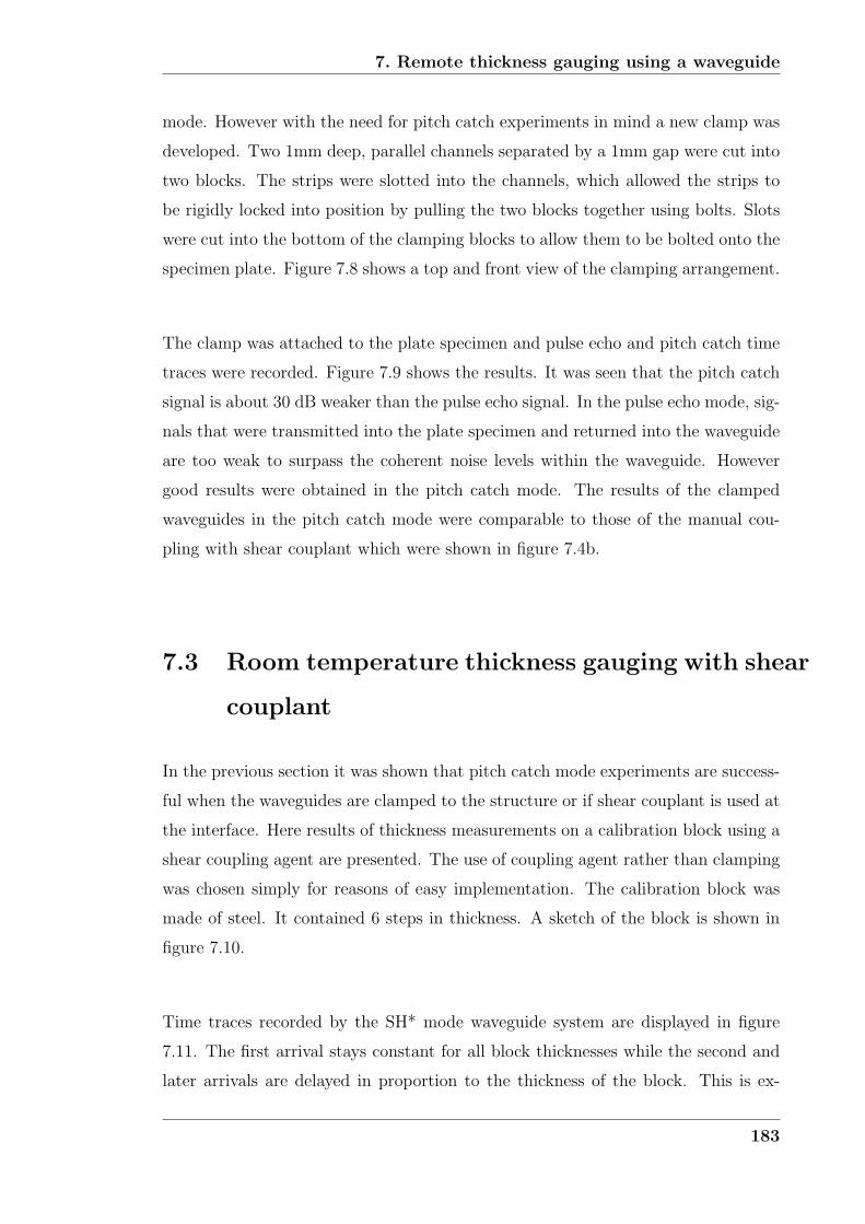
7. Remote thickness gauging using a waveguide
mode. However with the need for pitch catch experiments in mind a new clamp was
developed. Two 1mm deep, parallel channels separated by a 1mm gap were cut into
two blocks. The strips were slotted into the channels, which allowed the strips to
be rigidly locked into position by pulling the two blocks together using bolts. Slots
were cut into the bottom of the clamping blocks to allow them to be bolted onto the
specimen plate. Figure 7.8 shows a top and front view of the clamping arrangement.
The clamp was attached to the plate specimen and pulse echo and pitch catch time
traces were recorded. Figure 7.9 shows the results. It was seen that the pitch catch
signal is about 30 dB weaker than the pulse echo signal. In the pulse echo mode, sig-
nals that were transmitted into the plate specimen and returned into the waveguide
are too weak to surpass the coherent noise levels within the waveguide. However
good results were obtained in the pitch catch mode. The results of the clamped
waveguides in the pitch catch mode were comparable to those of the manual cou-
pling with shear couplant which were shown in figure 7.4b.
7.3 Room temperature thickness gauging with shear
couplant
In the previous section it was shown that pitch catch mode experiments are success-
ful when the waveguides are clamped to the structure or if shear couplant is used at
the interface. Here results of thickness measurements on a calibration block using a
shear coupling agent are presented. The use of coupling agent rather than clamping
was chosen simply for reasons of easy implementation. The calibration block was
made of steel. It contained 6 steps in thickness. A sketch of the block is shown in
figure 7.10.
Time traces recorded by the SH* mode waveguide system are displayed in figure
7.11. The first arrival stays constant for all block thicknesses while the second and
later arrivals are delayed in proportion to the thickness of the block. This is ex-
183
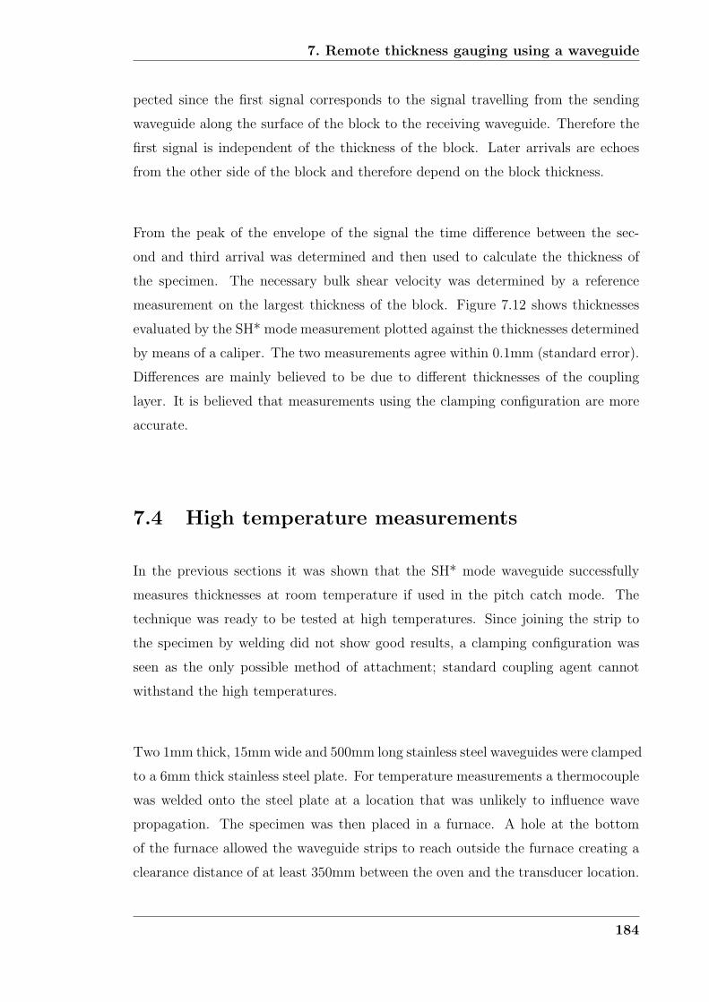
7. Remote thickness gauging using a waveguide
pected since the first signal corresponds to the signal travelling from the sending
waveguide along the surface of the block to the receiving waveguide. Therefore the
first signal is independent of the thickness of the block. Later arrivals are echoes
from the other side of the block and therefore depend on the block thickness.
From the peak of the envelope of the signal the time difference between the sec-
ond and third arrival was determined and then used to calculate the thickness of
the specimen. The necessary bulk shear velocity was determined by a reference
measurement on the largest thickness of the block. Figure 7.12 shows thicknesses
evaluated by the SH* mode measurement plotted against the thicknesses determined
by means of a caliper. The two measurements agree within 0.1mm (standard error).
Differences are mainly believed to be due to different thicknesses of the coupling
layer. It is believed that measurements using the clamping configuration are more
accurate.
7.4 High temperature measurements
In the previous sections it was shown that the SH* mode waveguide successfully
measures thicknesses at room temperature if used in the pitch catch mode. The
technique was ready to be tested at high temperatures. Since joining the strip to
the specimen by welding did not show good results, a clamping configuration was
seen as the only possible method of attachment; standard coupling agent cannot
withstand the high temperatures.
Two 1mm thick, 15mm wide and 500mm long stainless steel waveguides were clamped
to a 6mm thick stainless steel plate. For temperature measurements a thermocouple
was welded onto the steel plate at a location that was unlikely to influence wave
propagation. The specimen was then placed in a furnace. A hole at the bottom
of the furnace allowed the waveguide strips to reach outside the furnace creating a
clearance distance of at least 350mm between the oven and the transducer location.
184
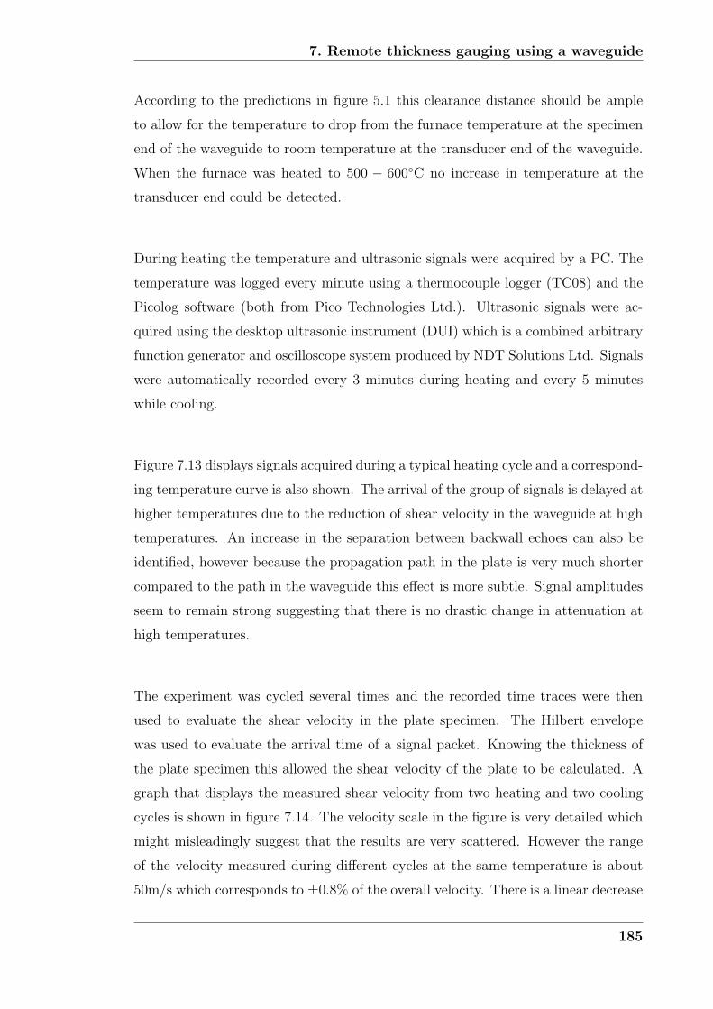
7. Remote thickness gauging using a waveguide
According to the predictions in figure 5.1 this clearance distance should be ample
to allow for the temperature to drop from the furnace temperature at the specimen
end of the waveguide to room temperature at the transducer end of the waveguide.
When the furnace was heated to 500 − 600◦C no increase in temperature at the
transducer end could be detected.
During heating the temperature and ultrasonic signals were acquired by a PC. The
temperature was logged every minute using a thermocouple logger (TC08) and the
Picolog software (both from Pico Technologies Ltd.). Ultrasonic signals were ac-
quired using the desktop ultrasonic instrument (DUI) which is a combined arbitrary
function generator and oscilloscope system produced by NDT Solutions Ltd. Signals
were automatically recorded every 3 minutes during heating and every 5 minutes
while cooling.
Figure 7.13 displays signals acquired during a typical heating cycle and a correspond-
ing temperature curve is also shown. The arrival of the group of signals is delayed at
higher temperatures due to the reduction of shear velocity in the waveguide at high
temperatures. An increase in the separation between backwall echoes can also be
identified, however because the propagation path in the plate is very much shorter
compared to the path in the waveguide this effect is more subtle. Signal amplitudes
seem to remain strong suggesting that there is no drastic change in attenuation at
high temperatures.
The experiment was cycled several times and the recorded time traces were then
used to evaluate the shear velocity in the plate specimen. The Hilbert envelope
was used to evaluate the arrival time of a signal packet. Knowing the thickness of
the plate specimen this allowed the shear velocity of the plate to be calculated. A
graph that displays the measured shear velocity from two heating and two cooling
cycles is shown in figure 7.14. The velocity scale in the figure is very detailed which
might misleadingly suggest that the results are very scattered. However the range
of the velocity measured during different cycles at the same temperature is about
50m/s which corresponds to ±0.8% of the overall velocity. There is a linear decrease
185

7. Remote thickness gauging using a waveguide
in velocity from ∼ 3100m/s at room temperature to ∼ 2750m/s at 600◦C, which
represents about 10% of the overall velocity.
In the above calculation the thermal expansion of the material in the furnace and
the corresponding thickness change has been neglected. For stainless steel Kaye and
Laby [62] quote an expansion coefficient of 19.7 ∗10−6/K at a temperature of 500◦C.
Below this temperature the expansion coefficient is slightly less and above slightly
higher. Using a round figure of 20 ∗ 10−6/K for the whole 600◦C the expected thick-
ness change due to heating is about 1.2%. Therefore the path that the ultrasonic
wave travels and the evaluated velocity is also expected to change by ∼ 1.2%. Com-
pared to the measured 10% decrease in velocity the change in thickness and velocity
due to thermal expansion of ∼ 1.2% is therefore believed to be negligible.
The furnace was kept running at a temperature of 500◦C for a period of four weeks to
demonstrate the long-term stability of the monitoring system. The temperature was
monitored every hour to ensure continuity, and temperature and ultrasonic sample
traces were recorded every 12 hours. The first and the last collected time traces
are shown in figure 7.15. Signal amplitudes increased with time and better signals
were achieved after long periods at high temperature. This is believed to be due to
changes that occur at the waveguide/specimen junction. High clamping pressures
and the increased temperature seem to improve ultrasonic shear wave transmission
through the joint which leads to the conclusion that long term monitoring at high
temperatures is possible.
7.5 Summary
In the previous sections the attachment of a strip waveguide to a plate specimen
was investigated in order to find a joining method that allows clean transmission
and reception of the SH* mode into and from the plate. Manual coupling with
shear coupling agent, permanent attachment methods like welding or soldering and
186
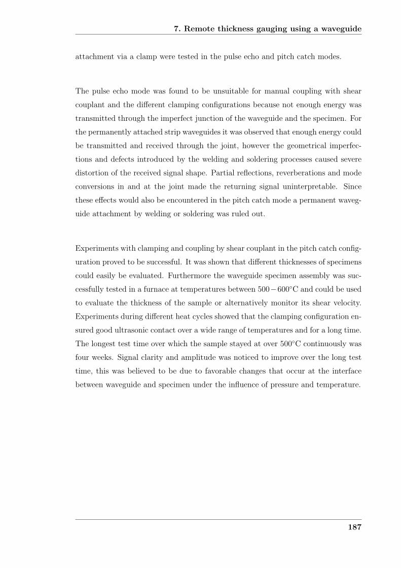
7. Remote thickness gauging using a waveguide
attachment via a clamp were tested in the pulse echo and pitch catch modes.
The pulse echo mode was found to be unsuitable for manual coupling with shear
couplant and the different clamping configurations because not enough energy was
transmitted through the imperfect junction of the waveguide and the specimen. For
the permanently attached strip waveguides it was observed that enough energy could
be transmitted and received through the joint, however the geometrical imperfec-
tions and defects introduced by the welding and soldering processes caused severe
distortion of the received signal shape. Partial reflections, reverberations and mode
conversions in and at the joint made the returning signal uninterpretable. Since
these effects would also be encountered in the pitch catch mode a permanent waveg-
uide attachment by welding or soldering was ruled out.
Experiments with clamping and coupling by shear couplant in the pitch catch config-
uration proved to be successful. It was shown that different thicknesses of specimens
could easily be evaluated. Furthermore the waveguide specimen assembly was suc-
cessfully tested in a furnace at temperatures between 500−600◦C and could be used
to evaluate the thickness of the sample or alternatively monitor its shear velocity.
Experiments during different heat cycles showed that the clamping configuration en-
sured good ultrasonic contact over a wide range of temperatures and for a long time.
The longest test time over which the sample stayed at over 500◦C continuously was
four weeks. Signal clarity and amplitude was noticed to improve over the long test
time, this was believed to be due to favorable changes that occur at the interface
between waveguide and specimen under the influence of pressure and temperature.
187
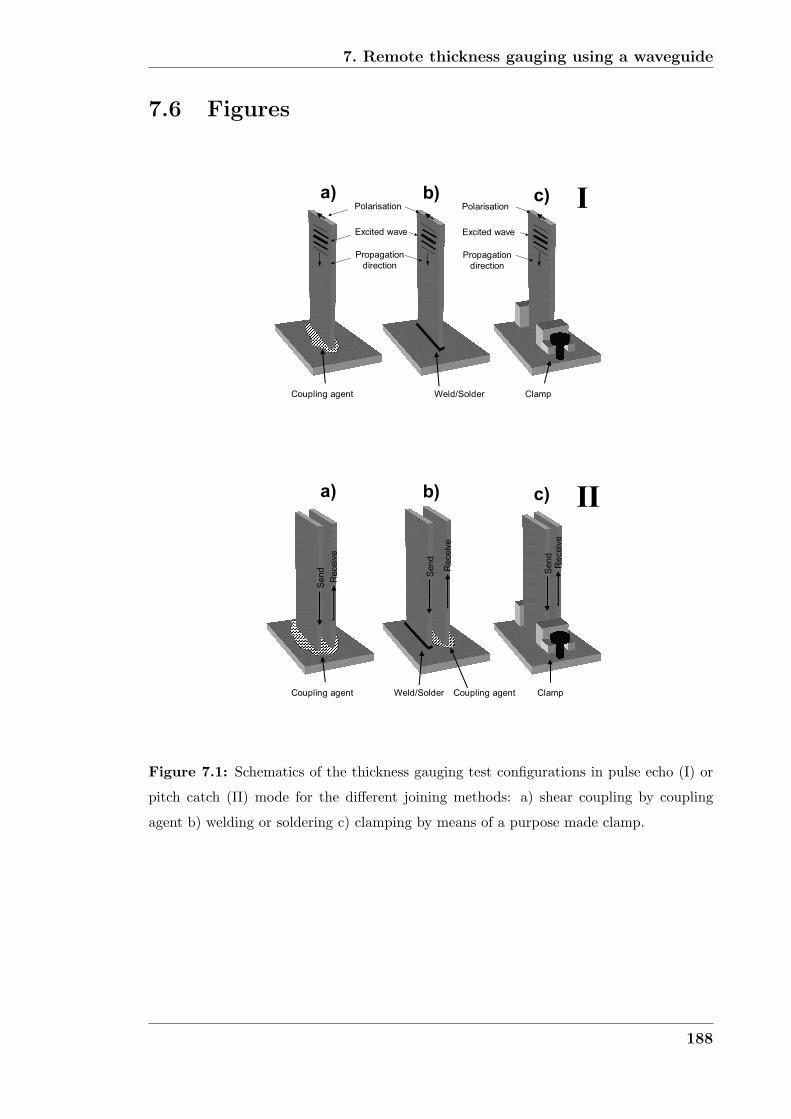
7. Remote thickness gauging using a waveguide
7.6 Figures
� �
����������� �� ���� � �����
�� �� ��������������
����� ����
����������
�������
������������
����� ����
����������
�������
�
� �
����������� �� ���� � �����
�� �� ��
�����������
��
���� ��
��
���� ��
��
���� ��
��
Figure 7.1: Schematics of the thickness gauging test configurations in pulse echo (I) or
pitch catch (II) mode for the different joining methods: a) shear coupling by coupling
agent b) welding or soldering c) clamping by means of a purpose made clamp.
188
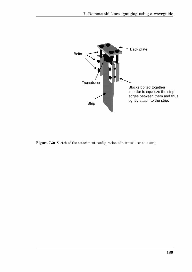
7. Remote thickness gauging using a waveguide
� �
�����
����� �������������
���������������������������
������ ���������������������
��������������������������
���������
����
���������
Figure 7.2: Sketch of the attachment configuration of a transducer to a strip.
189
7. Remote thickness gauging using a waveguide
178 180 182 184 186 188 190-2
-1
0
1
2
Am
plit
ud
e (
V)
178 180 182 184 186 188 190-2
-1
0
1
2
Time ( s)
Am
plit
ud
e (
V)
a)
b)
Figure 7.3: SH* mode pulse echo signal received through a 1mm thick and 15mm wide
steel strip coupled to a 6mm thick steel plate: a) signal before coupling b) signal when
strip is manually pushed onto the treacle covered steel plate surface.
190
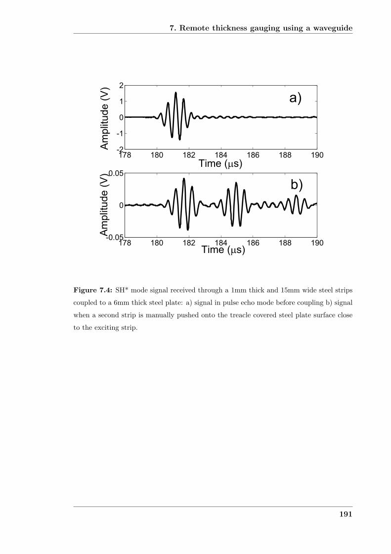
7. Remote thickness gauging using a waveguide
178 180 182 184 186 188 190-2
-1
0
1
2
178 180 182 184 186 188 190-0.05
0
0.05
a)
b)
Time ( s)
Am
plit
ud
e (
V)
Am
plit
ud
e (
V)
Time ( s)
Figure 7.4: SH* mode signal received through a 1mm thick and 15mm wide steel strips
coupled to a 6mm thick steel plate: a) signal in pulse echo mode before coupling b) signal
when a second strip is manually pushed onto the treacle covered steel plate surface close
to the exciting strip.
191
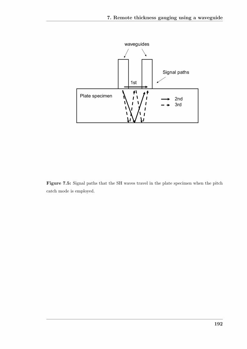
7. Remote thickness gauging using a waveguide
� �
���
���
��
��� ����
�������������
����������
Figure 7.5: Signal paths that the SH waves travel in the plate specimen when the pitch
catch mode is employed.
192

7. Remote thickness gauging using a waveguide
190 195 200 205 210 215 220 225
-2
0
2
Time ( s)
Am
plit
ud
e (
V)
190 195 200 205 210 215 220 225-1
-0.5
0
0.5
1
Time ( s)
Am
plit
ud
e (
V)
a)
b)
Figure 7.6: SH* mode pulse echo signal received through a 1mm thick and 15mm wide
steel strip welded to a 6mm thick steel plate: a) signal before welding b) signal after
welding.
193
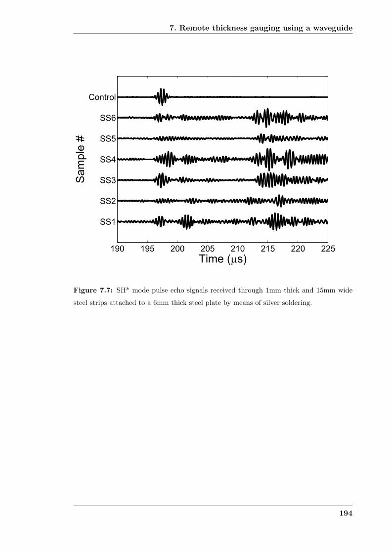
7. Remote thickness gauging using a waveguide
190 195 200 205 210 215 220 225
SS1
SS2
SS3
SS4
SS5
SS6
Control
Time ( s)
Sa
mp
le #
Figure 7.7: SH* mode pulse echo signals received through 1mm thick and 15mm wide
steel strips attached to a 6mm thick steel plate by means of silver soldering.
194
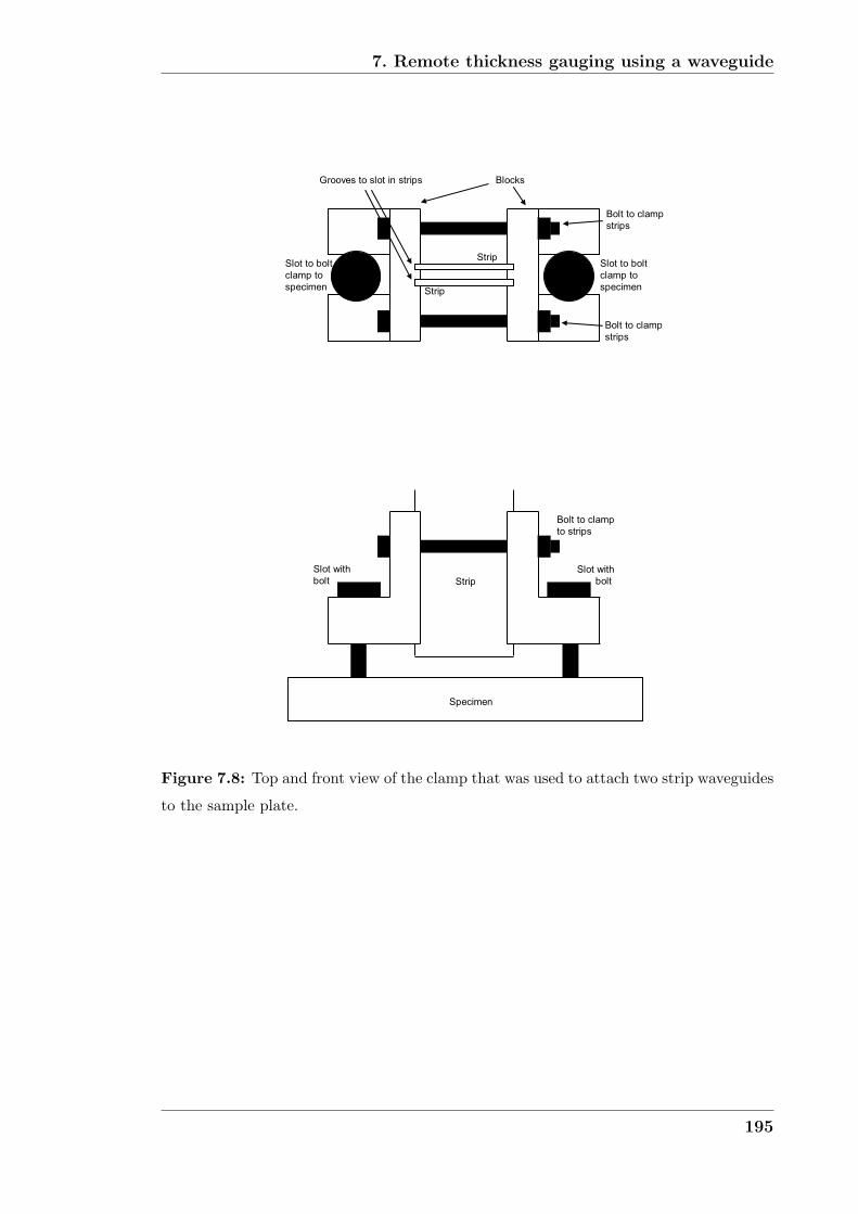
7. Remote thickness gauging using a waveguide
� �
�����
�����������������
������
�������
�����������
������
�����
������������
������
�������
�������������������������
�����������
������
� �
�!�������
��!���!�������
��!�������
������
��!������!���
���������
Figure 7.8: Top and front view of the clamp that was used to attach two strip waveguides
to the sample plate.
195
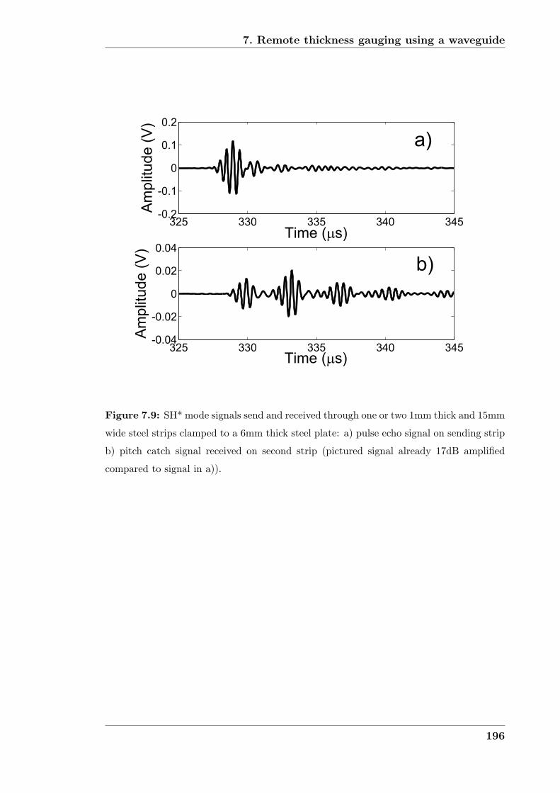
7. Remote thickness gauging using a waveguide
325 330 335 340 345-0.2
-0.1
0
0.1
0.2
Time ( s)
Am
plit
ud
e (
V)
325 330 335 340 345-0.04
-0.02
0
0.02
0.04
Time ( s)
Am
plit
ud
e (
V)
a)
b)
Figure 7.9: SH* mode signals send and received through one or two 1mm thick and 15mm
wide steel strips clamped to a 6mm thick steel plate: a) pulse echo signal on sending strip
b) pitch catch signal received on second strip (pictured signal already 17dB amplified
compared to signal in a)).
196
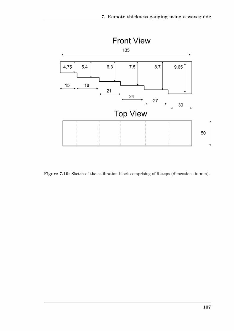
7. Remote thickness gauging using a waveguide
� �
����� �����
�� ��
��
����
��
���� ��� ��� ��� ��
��
��� ���
����
Figure 7.10: Sketch of the calibration block comprising of 6 steps (dimensions in mm).
197
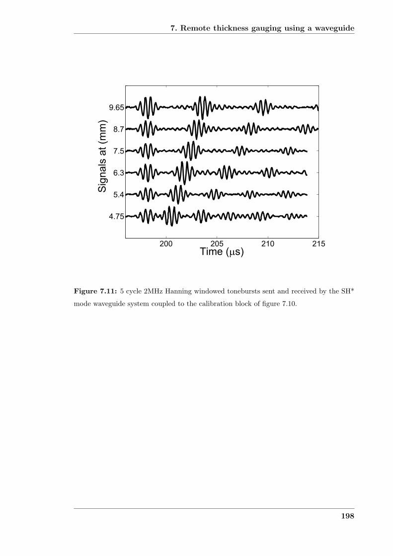
7. Remote thickness gauging using a waveguide
200 205 210 215
4.75
5.4
6.3
7.5
8.7
9.65
Time ( s)
Sig
na
ls a
t (m
m)
Figure 7.11: 5 cycle 2MHz Hanning windowed tonebursts sent and received by the SH*
mode waveguide system coupled to the calibration block of figure 7.10.
198
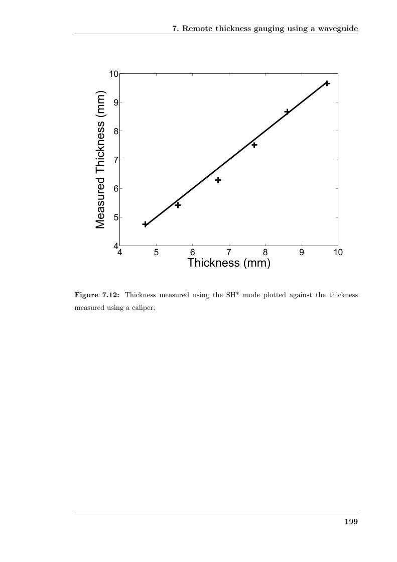
7. Remote thickness gauging using a waveguide
4 5 6 7 8 9 104
5
6
7
8
9
10
Thickness (mm)
Me
asu
red
Th
ickn
ess (
mm
)
Figure 7.12: Thickness measured using the SH* mode plotted against the thickness
measured using a caliper.
199
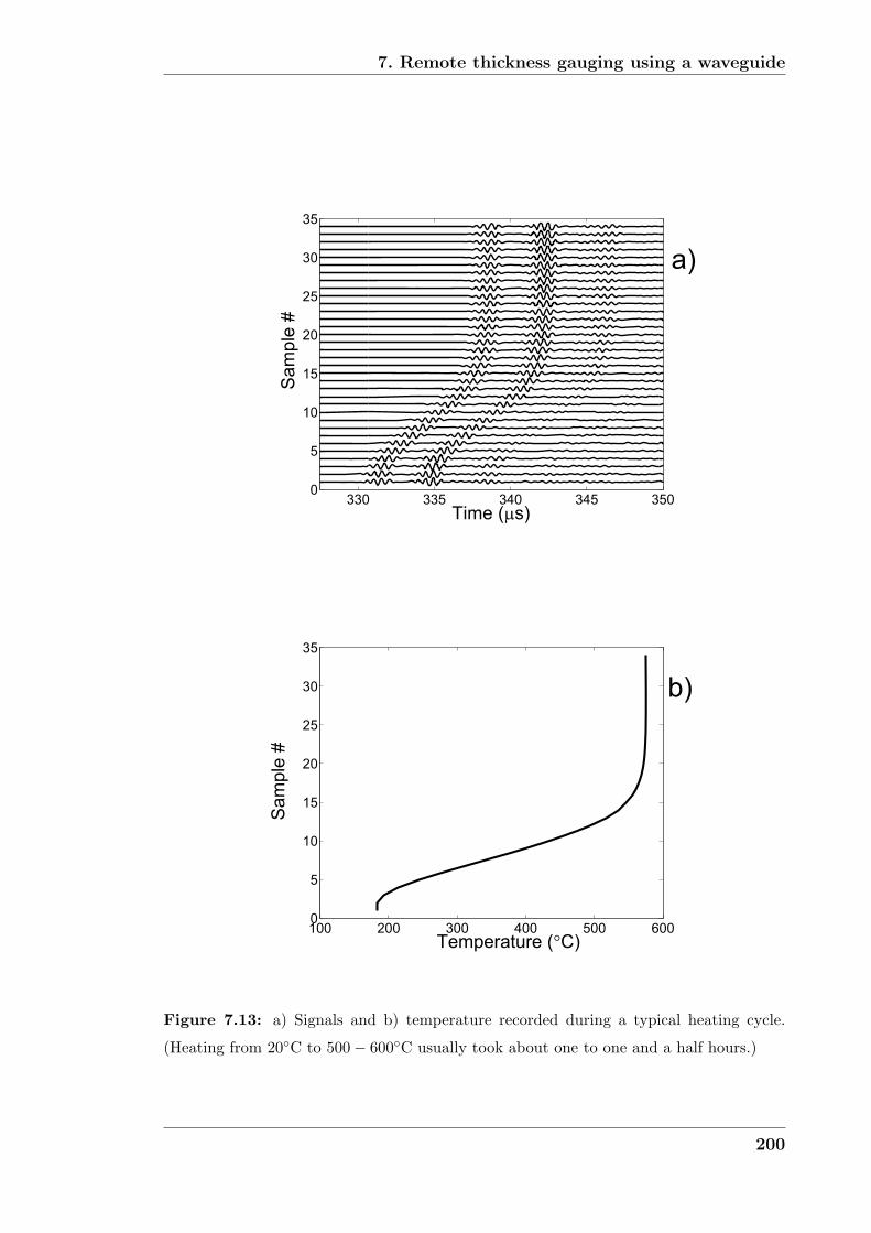
7. Remote thickness gauging using a waveguide
330 335 340 345 3500
5
10
15
20
25
30
35
Time ( s)
Sa
mp
le #
a)
100 200 300 400 500 6000
5
10
15
20
25
30
35
Temperature ( C)
Sa
mp
le #
b)
Figure 7.13: a) Signals and b) temperature recorded during a typical heating cycle.
(Heating from 20◦C to 500 − 600◦C usually took about one to one and a half hours.)
200
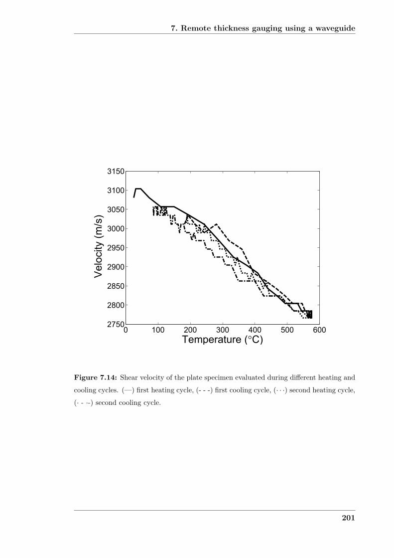
7. Remote thickness gauging using a waveguide
0 100 200 300 400 500 6002750
2800
2850
2900
2950
3000
3050
3100
3150
Temperature ( C)
Ve
locity (
m/s
)
Figure 7.14: Shear velocity of the plate specimen evaluated during different heating and
cooling cycles. (—) first heating cycle, (- - -) first cooling cycle, (· · ·) second heating cycle,
(· - ·-) second cooling cycle.
201
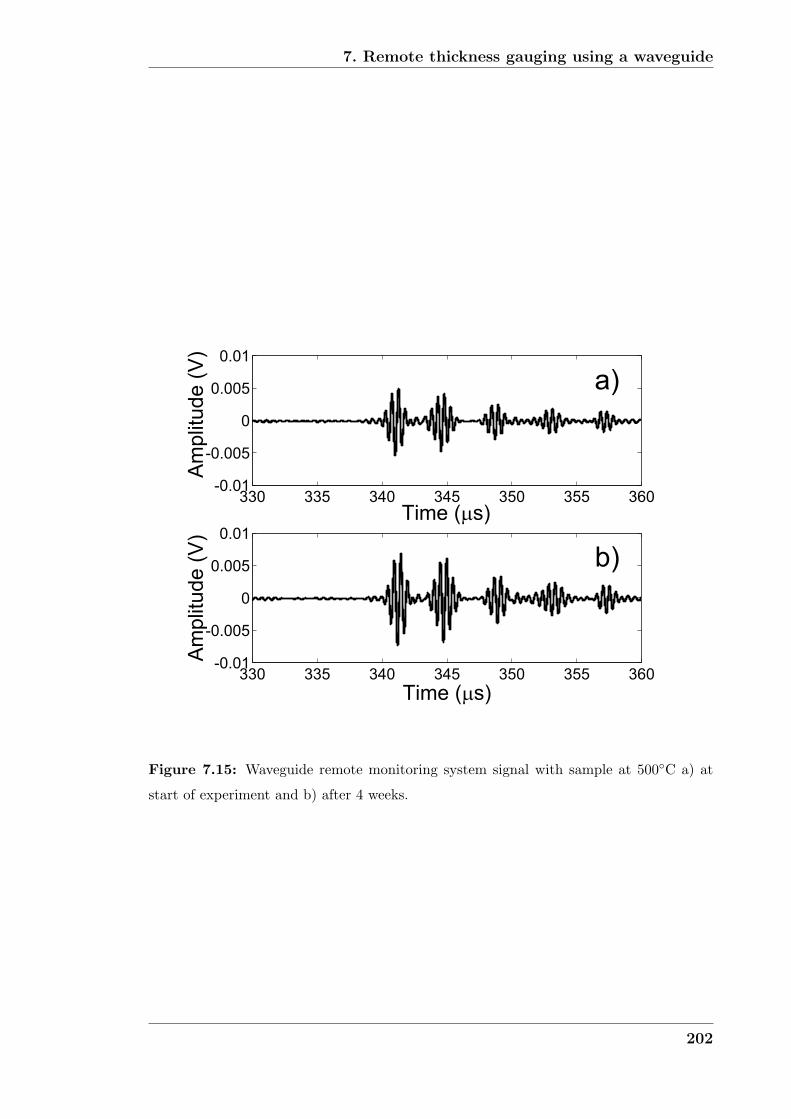
7. Remote thickness gauging using a waveguide
330 335 340 345 350 355 360-0.01
-0.005
0
0.005
0.01
Time ( s)
Am
plit
ud
e (
V)
330 335 340 345 350 355 360-0.01
-0.005
0
0.005
0.01
Time ( s)
Am
plit
ud
e (
V)
a)
b)
Figure 7.15: Waveguide remote monitoring system signal with sample at 500◦C a) at
start of experiment and b) after 4 weeks.
202
Chapter 8
Conclusions
8.1 Thesis Review
In this thesis the use of guided waves for fluid property measurements and remote
structural monitoring was investigated. The use of guided ultrasonic waves offers
several advantages over conventional techniques: for the application of fluid prop-
erty measurements the need for a test cell is removed and beam spreading effects
are avoided. For remote structural monitoring the waveguide allows the transducer
to be situated at a distance from the object that is being monitored. This makes
it possible to monitor structures in harsh environments which standard transducers
could not withstand.
Existing guided wave techniques for fluid property measurements use the effect of
leakage or an entry reflection to evaluate the bulk and shear modulus of an embed-
ding medium. These methods however do not allow the evaluation of attenuation
in the surrounding material. Therefore in this thesis an interface wave, called the
quasi-Scholte mode, was used for fluid bulk property measurements. The quasi-
Scholte mode propagates in both the fluid and the waveguide; however its energy
is mainly trapped at the interface between the waveguide and the fluid and decays
away with distance from the waveguide surface. The interface wave is sensitive to
all of the fluid properties.
203
8. Conclusions
In chapter 3 the theory behind the Scholte and quasi-Scholte wave was described.
Then in chapter 4 a series of experiments using the quasi-Scholte mode to measure
fluid properties was discussed. Some of the outcomes of chapter 4 suggested that it
would be beneficial to reduce the width of the plate waveguide as far as possible in
order to reduce errors. When the propagating wave modes in a strip were analysed,
in addition to an A0* mode that is suitable for exciting the quasi-Scholte mode, a
non-dispersive shear horizontal mode was also found. This mode was termed the
SH* mode and it was realised that it could be used for remote inspection of struc-
tures in extreme environments.
Chapter 5 concentrated on investigating the characteristics of wave propagation in
strips of rectangular cross section. It described the techniques used to obtain dis-
persion curves for rectangular waveguides and presented results for steel strips.
A challenging problem is the transfer of the wave from the waveguide into the object
that is to be investigated. The analysis of the wave propagation in the waveguide
and the object was uncoupled by considering the stresses transmitted by the guided
wave mode as a surface load on the test piece. A collection of literature results for
the radiation characteristics of surface sources on half spaces was therefore consid-
ered in chapter 6.
The theoretical findings of chapters 5 and 6 were used to devise an experimental
setup to carry out remote thickness gauging using a waveguide. Experiments eval-
uating different waveguide-structure joints were carried out. Successful thickness
gauging experiments on calibration blocks of different thicknesses were also per-
formed to validate the capabilities of the waveguide sensor. Long-term tests at high
temperatures (up to 600◦C) as well as temperature cycling were also carried out to
verify the robustness of the setup and to show that long term monitoring at high
temperatures using a waveguide is possible.
204
8. Conclusions
8.2 Findings
The work presented in this thesis revealed further insight into the working principles
of ultrasonic waveguide sensors and their potential applications. The modelling of
the quasi-Scholte wave and the construction of a fluid property sensor lead to a
good understanding of the interface wave and its capabilities and limitations when
used to extract fluid properties. A general summary of the findings related to the
quasi-Scholte mode will be given first before findings from the remote waveguide
monitoring system are recalled.
8.2.1 Fluid property measurements using the quasi-Scholte
mode
The theoretical investigation into the quasi-Scholte wave showed that the fraction
of its energy that travels in the fluid depends on the ratios of the fluid density and
bulk velocity to the solid density and bulk velocity. The same is true for the Scholte
wave velocity, which is the velocity that the quasi-Scholte mode asymptotes to at
high frequency thickness products. Therefore to be sensitive to the fluid the right
waveguide material for a certain fluid will have to be chosen. Most fluids are aqueous
solutions for which steel is a suitable waveguide material. Over 99% of the Scholte
wave energy on a steel/water interface is located in the fluid.
The energy distribution between waveguide material and fluid also depends on the
operating frequency-thickness product. At low frequency-thicknesses all the energy
is located in the waveguide while at higher frequency-thickness products most of
the energy travels in the fluid. Sensitivity to the fluid is generally best at high
frequency thickness products with the exception of the quasi-Scholte mode group
velocity which is most sensitive to the fluid bulk velocity at frequency thickness
products around 350kHz-mm (for steel in aqueous fluids). The group velocity of
the quasi-Scholte mode at this frequency-thickness product can be three times more
sensitive than a conventional bulk velocity measurement. However the sensitivity
205
8. Conclusions
to fluid bulk attenuation is not as high and is expected to perform worse than a
measurement in a test cell.
Two attenuation mechanisms of the quasi-Scholte mode were identified. Shear leak-
age attenuates the interface wave due to in-plane surface displacements of the waveg-
uide that set up energy dissipating bulk shear waves in the fluid. The quasi-Scholte
mode is also attenuated by energy scattered or dissipated in the component of the
wave that travels in the fluid. This part of the attenuation is related to the fluid
bulk attenuation and can be used to evaluate the latter if isolated from the shear
leakage.
The excitation method presented excited the quasi-Scholte mode from the plate; it
is therefore not very effective at high frequency thickness products. An optimum
frequency window in which the quasi-Scholte mode is sensitive to fluid properties
and can be excited by a mode conversion from the A0 mode in a free waveguide was
found to lie around 200 − 500kHz mm for steel.
The experiments showed that bulk velocity measurements can be performed to
within 0.5%. For simple Newtonian fluids the viscosity can also be determined with
errors of up to 8%. Bulk attenuation measurements showed poorer performance
(∼ 20% error), which could partly be explained by lower sensitivity, geometrical de-
fects in the setup and the inversion problem being ill-posed. However improvements
in performance are possible and it is believed that a successful strategy to achieve
this would be the optimisation of the geometry of the measurement apparatus.
Possible applications of a quasi-Scholte mode ’dipstick’ could be the monitoring or
measurement of fluid bulk velocities in manufacturing processes or the use as rapid
testing equipment for bulk materials. Since the transducer is separated from the
sensing area, measurements in hot fluids are possible. The quasi-Scholte mode is
also well suited for applications such as fluid level sensing. Attenuation measure-
ment based applications like particle sizing are difficult to carry out with the current
206

8. Conclusions
quasi-Scholte mode setup due to the poor accuracy and the need for a large frequency
bandwidth. However where the differences between viscosity induced attenuation
and fluid bulk attenuation have to be detected the sensor is very useful.
8.2.2 Remote monitoring using a flexible waveguide
The investigation into an ’acoustic cable’ for remote ultrasonic monitoring of struc-
tures in harsh environments was focused on three different issues. The first was the
design of a non-dispersive waveguide, secondly the waveguide source characteristics
had to be optimised and finally a practical implementation of the best possible sys-
tem had to be found.
Even though not absolutely necessary the use of non-dispersive wave propagation
in the ’acoustic cable’ considerably reduces the complexity of the excitation system.
The traditional approach of reducing the frequency-thickness product of the waveg-
uide in order to operate in a region where the fundamental compressional wave mode
in the waveguide is non-dispersive was overcome by using a shear horizontal (SH*)
type mode in a very thin and wide rectangular strip. The strip mode possesses
a cut-off at low frequency-width products; however at high frequency-width prod-
ucts, the SH* mode becomes non-dispersive and asymptotes to the shear velocity
of the waveguide material. The mode shape of the SH* mode is constant through
the thickness of the strip and varies across the width in an approximately parabolic
fashion. The displacements are at a maximum in the centre of the strip and very
small on the strip edges, so that most of the energy travels along the centre of the
strip. Experimentally the SH* mode could reliably and selectively be excited with
an amplitude 30 dB above other undesirable modes.
When studying the literature on source characteristics on a half space an anti-plane
shear source was identified to have the best radiation characteristics. In the 2D limit
of a source of infinite length, which is approximated by the large aspect ratios of the
strip, advantages of the SH source are the excitation of only SH waves in the half
207
8. Conclusions
space: no compressional or surface waves are excited by an ideal SH line source. The
SH source cylindrically spreads in all directions and thus has a wide field of view.
When returning to the waveguide, SH waves in the half space excite the SH* mode
which propagates the signal back to the transducer. Other waveguide sources such
as circular, torsional sources would produce waves that on return to the waveguide
excite different modes from those that created them (flexural modes in this case).
Normal and tangential loading on the half space produces shear, compressional and
surface waves which considerably complicate the analysis. Furthermore the energy
content in the surface wave excited by normal or tangential sources is always very
large; this makes subsurface inspection very difficult.
An experimental study into the joining method revealed that although they trans-
mit most of the wave energy into the structure, permanent attachment methods are
not reliable. Features that are inevitably introduced by the joining process distort
the signal shape and cause reflections that greatly complicate the interpretation
of results. Other methods could only be successfully employed in the pitch catch
mode. While coupling with shear couplant is not possible at high temperatures its
use for thickness gauging experiments at room temperature was possible. Clamping
with a purpose made clamp showed good results, both at low and high temperatures.
A test system was successfully run at high temperatures for a period of over 4 weeks.
Several heating and cooling cycles after the period at constant high temperature also
did not deteriorate the strength or shape of signals. The shear velocity drops by
about 10% with increase of temperature from room temperature to around 600◦C
and must be corrected for if measurements are to be taken at different temperatures.
Experimentally, no issues with increased shear wave attenuation at high tempera-
tures (up to 600◦C) were encountered.
208

8. Conclusions
8.3 Future work
In future a detailed study of the quasi-Scholte mode attenuation of a rectangular
strip waveguide should be carried out in order to improve the quality of the bulk
attenuation measurements that are possible using the QS-mode. The addition of a
torsional wave sensor that allows the evaluation of fluid density at the same time
as a fluid bulk velocity and attenuation measurement would allow the guided wave
sensor to completely characterise the acoustic properties of a fluid. This is not com-
monly achieved by conventional ultrasonic test cells. The characterisation of hot
fluids using the QS mode should also be investigated.
The study of the remote waveguide monitoring sensor has opened many interesting
possibilities for further investigations. The effect of uneven or rough reflectors on
either side of the structure of the waveguide will have to be researched. This simu-
lates the effects of corrosion or erosion that are most likely encountered in real life
situations.
Another field to be explored is the use of the ’acoustic cable’ for defect (crack size)
monitoring over long periods and at elevated temperatures. For this it might be
useful to use the time of flight diffraction technique. Alternatively the construction
of arrays of strips and array techniques for monitoring the structure beneath the
waveguides could be employed. This would require a detailed study of the three
dimensional wave field produced by the SH* strip source.
209
Appendix A
Global Matrix Solution
In the global matrix method a matrix of the general solutions of wave propagation in
the system materials is set up with the appropriate boundary conditions (continuity
of stresses and displacements at boundaries). The system of equations results in an
eigenvalue/eigenvector problem that can be solved. The matrix equation for a plate
immersed in two half spaces of viscous fluid is given below. For more details see also
References [53], [23] and [22].
[A
]·
⎛⎜⎜⎜⎜⎜⎜⎜⎜⎜⎜⎜⎜⎜⎜⎜⎜⎝
Lf−
Tf−
Ls+
Ls−
Ts+
Ts−
Lf+
Tf+
⎞⎟⎟⎟⎟⎟⎟⎟⎟⎟⎟⎟⎟⎟⎟⎟⎟⎠
= 0 (A.1)
Where L and T are the amplitudes of the partial longitudinal and transverse waves.
The subscripts f and s refer to the fluid and solid respectively and the + and - signs
indicate the direction of the partial wave. Terminology here is from Lowe [23]. The
matrix A is: A = [B...C], where
210

A. Global Matrix Solution
B =
⎡⎢⎢⎢⎢⎢⎢⎢⎢⎢⎢⎢⎢⎢⎢⎢⎢⎣
k −k2Tf k kgSL
−k2Lf −k k2Ls −k2LsgSL
iρfBf 2iρfβ2fkk2Tf iρsBs iρsBsgSL
−2iρfβ2fkk2Lf iρfBf 2iρsβ
2skk2Ls −2iρsβ
2skk2LsgSL
0 0 kgSL k
0 0 k2LsgSL −k2Ls
0 0 iρsBsgSL iρsBs
0 0 2iρsβ2skk2LsgSL −2iρsβ
2skk2Ls
⎤⎥⎥⎥⎥⎥⎥⎥⎥⎥⎥⎥⎥⎥⎥⎥⎥⎦
(A.2)
C =
⎡⎢⎢⎢⎢⎢⎢⎢⎢⎢⎢⎢⎢⎢⎢⎢⎢⎣
k2Ts −k2TsgST 0 0
−k −kgST 0 0
−2iρsβ2skk2Ts 2iρsβ
2skk2TsgST 0 0
iρsBs iρsBsgST 0 0
k2TsgSS −k2Ts k k2Tf
−kgST −k k2Lf −k
−2iρsβ2skk2TsgST 2iρsβ
2skk2Ts iρfBf −2iρfβ
2fkk2Tf
iρsBsgST iρsBs 2iρfβ2fkk2Lf iρfBf
⎤⎥⎥⎥⎥⎥⎥⎥⎥⎥⎥⎥⎥⎥⎥⎥⎥⎦
(A.3)
where k is the wavenumber of the guided wave to be solved for, ρs is the solid plate
material density, ρf is the fluid density and the remaining quantities are defined by
the following equations:
k2Lf,s = ±(ω2
α2f,s
− k2)1/2 (A.4)
k2Tf,s = ±(ω2
β2f,s
− k2)1/2 (A.5)
Bf,s = ω2 − 2β2f,sk
2 (A.6)
GSL = ei(k2Lsh) (A.7)
GST = ei(k2Tsh) (A.8)
211
A. Global Matrix Solution
where k2Lf,s is the component of the longitudinal bulk wave wavenumber in the
direction normal to the plate surface, k2Tf,s is the component of the shear bulk wave
wavenumber in the direction normal to the plate surface, Bf,s, GSL and GST are
multiplication factors, h stands for the plate thickness. α and β are the complex
bulk velocities defined by:
αn =cl
1 − i κl
2π
(A.9)
βn =cs
1 − iκs
2π
(A.10)
The media are indicated by the subscripts f and s, which stand for fluid and solid
in the subscripts of other quantities.
The equations A.4 and A.5 contain a square root expression; this results in several
possible solutions, some of which may be unphysical (e.g. waves with negative
attenuation). Therefore care should be taken to chose the right sign of the expression
under the square root before entering equations A.4 and A.5 into matrix A.
A solution of equation A.1 exists if matrix A is singular, i.e. when the determinant
of the matrix equals zero. There are several wavenumbers that satisfy the equation
at each frequency. These are the different propagating modes that may exist. One of
these propagating modes is the quasi-Scholte mode. The complex wavenumber gives
the phase velocity ( ωkre
) and attenuation (kim) of the mode. By specifying one of the
partial wave amplitudes and substituting the complex wavenumber into equation
A.1 the mode shape can be determined at each frequency. The mode shape is the
distribution of displacements, stresses, strains and similar characteristics through
the cross section of the plate.
212
Appendix B
Derivation of an approximate
formula for the SH-wave
attenuation
The approach here follows closely the derivation of the approximate attenuation of
the longitudinal L(0,1) mode in [30]. The system that is described is a plate of
thickness h as shown in figure 3.16. The guided wave attenuation for a cross section
of a wave guide can be expressed by use of the average power flow:
α =∂P∂z
2Parea
(B.1)
Where Parea is the average power flow across the cross section of the waveguide, z
is the propagation direction. ∂P∂z
describes the energy leakage across the boundary
of the waveguide. We will first evaluate this term.
Assume a Newtonian fluid with appropriate relaxation time. The viscous skin depth
is defined as
δ = (2η/ρfω)1/2 (B.2)
Where η is the liquid viscosity, ρf the fluid density and ω the angular frequency.
Therefore an expression for the velocity in the liquid adjacent to the waveguide can
213
B. Derivation of an approximate formula for the SH-wave attenuation
be expressed as
v = v0exp(−y/δ) (B.3)
Where v0 denotes the surface velocity of the waveguide and y the distance from the
surface in the liquid.
The quantity ∂P∂z
, the change in average power flow, is the power leaving the waveg-
uide cross section. Therefore it is the dissipated power over a unit surface area. This
quantity is found by integrating the power flow per unit width of the plate across
the top and bottom surfaces of the plate
∂P
∂z= 2
∫ 1
0
1/2τ0v0dx (B.4)
where
τ0 = η∂v
∂y|y=0= −ηv0/δ (B.5)
and thus
∂P
∂z= −v2
0(ρfωη/2)1/2 (B.6)
The second quantity that has to be evaluated to find the guided wave attenuation
is the term Parea, the average power flow across the cross section of the plate. Using
the Poynting vector:
Parea =
∫ 1
0
∫ h
0
−v∗σ/2dydx (B.7)
214
B. Derivation of an approximate formula for the SH-wave attenuation
Where v∗ stands for the complex conjugate of the velocity and σ the stress at any
point within the cross section. The velocity and stress field variation can be de-
scribed using the displacement distribution for the SH mode [8]:
ux = Bei(kz−ωt) (B.8)
vx =dux
dt= −iωBei(kz−ωt) (B.9)
σx = Gdux
dz= ikBGei(kz−ωt) (B.10)
Hence,
Parea =
∫ 1
0
∫ h
0
ωkB2G
2dydx (B.11)
and using the identities k = ωc
and c =(
Gρs
)1/2
yields:
Parea = −1
2ω2B2(Gρs)
1/2h (B.12)
Now substituting the expression v0 = −iωB for the velocity at the interface into the
∂P∂z
term obtained earlier yields the guided wave attenuation:
α =∂P∂z
2Parea
=−v2
0(ηρf ω
2)1/2
−ω2B2(Gρs)1/2h(B.13)
after rearranging and cancellations,
α = − 1
2h
(2ρfωη
ρsG
)1/2
(B.14)
215
Appendix C
Phase and group velocity
Generally the solution to wave propagation problems results in an expression of the
form
u(x, t) = Aei(kx−ωt) (C.1)
where u is the displacement, A is the amplitude, k is the wavenumber of the wave,
x the spatial position of the wave along the propagation direction, ω is the angular
frequency and t the time. If the wavenumber k is allowed to be complex then
k = kr + iki (C.2)
with kr being the real part of the wavenumber and ki being the imaginary part of
the wavenumber. Using C.2 allows us to rewrite equation C.1
u(x, t) = Ae−kixei(krx−ωt) = Ae−αxei(krx−ωt) (C.3)
with ki the imaginary part of the wavenumber being equal to α, the attenuation of
the wave.
Equation C.3 now contains two separable terms, the first being Ae−αx that stands for
an amplitude that decays with propagation distance due to dissipative mechanisms,
216

C. Phase and group velocity
and the second term ei(krx−ωt) that expresses the harmonic oscillations of the wave
in time and space. The second term may be used to derive the phase velocity. For
propagation at constant phase the term in the brackets of the exponential has to
equal zero
(krx − ωt) = 0 (C.4)
thus
x
t=
ω
kr
= cp (C.5)
where cp is the phase velocity which describes the velocity at which the phase of the
wave travels through space.
Cheeke [96] recalls that wave propagation at a single carrier frequency does not
contain any information but the frequency of the wave. To transmit information
the carrier has to be modulated with another frequency. The combination of sev-
eral propagating frequencies forms a wave packet. The wave packet also propagates
through the medium but at the group velocity, which in general is different from
the phase velocity. A simple example for the derivation of group velocity of two
frequencies was shown by Stokes [97] and is also given in Rose [8]. Rose also gave
the following derivation of group velocity:
Consider the phase change of an individual frequency component at time increment
t = t0 + dt,
dPi = (ki(x0 + dx) − ωi(t0 + dt)) − (kix0 − ω0t) = kidx − ωidt (C.6)
now for the wave group to remain unchanged, the phase changes have to be the
same for all of its constituent frequency components, therefore
dPi − dPj = 0 or (ki − kj)dx − (ωi − ωj)dt = 0 (C.7)
217

C. Phase and group velocity
which can be rewritten as
dx
dt− dω
dk= 0 (C.8)
this defines the group velocity as
cg =dω
dk(C.9)
The group velocity is the velocity at which a wave packet moves through space
(strictly speaking the wave packet travels at the energy velocity [98] however if
the attenuation is low as in most real life cases the group velocity is a very good
approximation). As with the phase velocity, the group velocity can be frequency
dependent; actually the group velocity is a derivative of the wavenumber (and thus
also the phase velocity). When the velocities are functions of frequency, the wave
propagation is said to be dispersive. A wave packet is always made up of several
frequencies. In dispersive media each constituent frequency will travel at a specific
velocity. Therefore the shape of a wave packet will be distorted with increasing
propagation length. This is the most significant feature of dispersion.
Figure C.1 shows a plot of the phase and group velocities of the lowest order anti-
symmetric Lamb wave mode A0 of a 1mm thick steel plate as a function of frequency.
At low frequencies the mode is very dispersive, meaning that there is a relatively
steep velocity slope.
Figure C.2 shows simulated excitation signals and signals that have propagated
for 100mm as A0 mode (the signals were simulated using the DISPERSE software
[22]). Their frequency spectra are also shown. It can be seen that the signal in a)
is made up of a broad bandwidth of frequencies and therefore is distorted more as
the frequency components travel at different velocities and spread out. The signal
in b) has a rather narrow frequency bandwidth and disperses less with distance. In
Figure C.2 a) it can also be seen that the higher frequency components of the signal
arrive earlier than the low frequency components. This can be predicted from the
dispersion curve (C.1).
218
C. Phase and group velocity
C.1 Retrieving phase and group velocity from mea-
surements
The accurate retrieval of phase velocity and group velocity data from measurements
is of utmost importance in non-destructive testing applications. In relatively non-
dispersive media such as metals the characteristic velocity of the material is usually
obtained on a sample specimen. With the knowledge of the ultrasonic velocity
in the material other techniques such as thickness gauging or defect monitoring
can be used. In dispersive media, for example suspensions of particles in a liquid
or adhesives, the velocity dispersion itself contains information about the material
and can therefore be used for material characterization. An example of this is the
measurement of particle size distribution in suspensions [3]; other examples of fluid
characterization are well summarized in Povey’s book [1].
The measurement of phase velocity is usually based on the comparison of the phase
information of two signal pulses that have travelled over two different lengths in the
material. A standard procedure for this type of measurements is the phase spectrum
method [99]. Another similar method that does not rely on the temporal separation
of the two signals to be analyzed is the amplitude spectrum method [60]. In the
following section the theoretical background behind these two standard methods
will be recalled.
Consider a harmonic wave propagating in an unbound medium. The displacements
in the positive propagation directions can be expressed as follows
u(x, t) = Aei(ωt−kx−φ)e−αx (C.10)
where, u is the displacement, t is the time, x is the propagation distance, ω is
the frequency, α the attenuation and φ an arbitrary phase angle. Using Fourier
transformation and some algebra [60] this can be rewritten in the form
F (u(x, t)) = F (u(0, t))ei(−kx)e−αx (C.11)
where F indicates a Fourier transformed entity. In this case the wavenumber k and
the attenuation α are real. The factor e−αx will therefore not influence the phase
219

C. Phase and group velocity
of the signal but only its amplitude. The signal amplitude can be calculated at two
different positions as
F (u(x1, t)) = F (u(0, t))ei(−kx1)e−αx1 (C.12)
F (u(x2, t)) = F (u(0, t))ei(−kx2)e−αx2 (C.13)
which when rewritten in the form of a magnitude and phase yields the following:
F (u(x1, t)) = A1ei(−kx1+φ01) = A1e
i(φ1) (C.14)
F (u(x2, t)) = A2ei(−kx2+φ02) = A2e
i(φ2) (C.15)
Now the difference in phase of the two signals at their respective positions allows
the phase velocity to be extracted.
dφ = φ2 − φ1 = −k(x2 − x1) (C.16)
but k = ωcp
, therefore
dφ = − ω
cp
(x2 − x1) and cp =ω(x2 − x1)
−dφ(C.17)
Equation C.17 gives a simple expression to evaluate the phase velocity from signals
collected at two position along a signal path. However there is a caveat. For the
simple expression to work accurately and reliably, the absolute phase difference at
each frequency has to be determined. From the signals the phase information will be
extracted in a wrapped form, this means that the phase will be limited to values in
the range of -π to π. The absolute phase however has to be in an unwrapped form.
The unwrapping of the signal causes a problem and is only possible in frequency
regions where a strong signal is present. Also unwrapping algorithms are not perfect
and an error of 2π can easily be introduced to the unwrapped phase. In cases where
the frequency spectrum does not contain any signal at low frequencies, the phase
information at low frequencies will be entirely made up of noise. This will make
it impossible to unwrap the phase and find the absolute unwrapped phase of the
signal.
220
C. Phase and group velocity
C.2 Retrieving phase velocity by cosine interpo-
lation
One of the main problems of methods using the phase spectrum method is the
phase uncertainty due to the wrapping from −π to +π. Further errors are also
introduced by errors in the distance measurement between two transducer locations.
If several transducers can be used to collect signals over a short distance (usually
less than a wavelength), or one transducer can be scanned over the surface, a cosine
interpolation can be used to accurately determine phase velocity. Here the approach
as used by Simonetti [100] is recalled. Consider the Fourier transform of a signal
that has been received at a reference position:
S(ω)ref = A(ω)ei(−kr(ω)xref )e−α(ω)xref (C.18)
where S is the received signal, A is the complex amplitude of the travelling wave,
kr is the real wavenumber of the wave, α is the attenuation of the wave and xref
the position at which the signal is received. Note here that all quantities except the
distance are frequency dependent. The signal at any other position (x1) along the
travelling path of the wave can be expressed as:
S(ω)1 = A(ω)ei(−kr(ω)x1)e−α(ω)x1 (C.19)
Now we can divide the first expression by the second to eliminate the effects of the
signal amplitude.
S(ω)ref
S(ω)1= e
i(−kr(ω)xref )
ei(−kr(ω)x1)e−α(ω)xref
e−α(ω)x1= ei(kr(ω)(x1−xref )e−(α(ω)(x1−xref )
= Fei(kr(ω)(x1−xref )
= F (cos(kr(ω)(x1 − xref )) − isin(kr(ω)(x1 − xref )))
(C.20)
where F is a real factor depending on the wave attenuation. Thus it can be concluded
that the real part of the signal ratio is related to the cosine of the wavenumber-
221

C. Phase and group velocity
distance product. By evaluating the real part of the signal ratio at different distances
from the reference signal the phase velocity can be found using a cosine interpolation.
R(S(ω)ref
S(ω)1
) = F (cos(kr(ω)(x1 − xref )) = F (cos(ω
Cph(ω)(x1 − xref )) (C.21)
Figure C.3 shows signals that have been created using the dispersion characteristics
of an A0 mode, determined using the DISPERSE software. The signals are 5 cycle
Hanning windowed tonebursts with a centre frequency of 500 kHz that have been
propagated over distances ranging from 100 to 105.5 mm from the source. The
signals were processed as described by the above procedure and a cosine interpolation
was carried out at the centre frequency. Figure C.4 shows the real part of the ratio
of the spectra of the different signals and the reference signal as well as the best
result of the cosine interpolation at the signal centre frequency of 500 kHz.
This method works very well and is very accurate provided the distance data is
available at a good enough accuracy. However a major drawback is the need of
a relatively large set of data to calculate the phase velocity, on average about 8
signals at different distances are needed. The method also only works well if the
interval between the scanning points of the signals is much less than a wavelength;
this avoids aliasing.
C.3 Group velocity measurement using the zero
phase slope
The author learned about the method of zero phase slope in private discussion
with Prof. Peter Nagy [101] who developed and used the method previously. The
fundamental idea behind the determination of group velocity using the zero phase
slope method is the evaluation of the Fourier transform of the signal within a window
that is swept over the time domain signal. When the window is aligned with the
group arrival time of a frequency component within the signal the phase slope of
the frequency component will tend to zero. Thus the group arrival time is evaluated
by sweeping a window over the time domain signal and evaluating the phase slope
for each frequency. At the zero phase slope point the window centre coincides with
222
C. Phase and group velocity
the frequency group arrival. This can be shown using the shift property of Fourier
transforms:
F (f(t)) =∫ +T
−Tf(t)e−iωtdt = F (ω)
F (f(t − tshift)) =∫ +T
−Tf(t − tshift)e
−iωtdt =
∫ +T
−Tf(t − tshift)e
−iω(t−tshift)e−iωtshiftd(t − tshift)
= e−iωtshiftF (ω)
(C.22)
Consider now the Fourier transform of the displacement signal of a travelling wave
F (u(x, t)) = F (ω)e−i(kx)e−iφ0 (C.23)
when the time origin of the signal is shifted to the right by a delay tshift the shift
property of the transform leads to the following expression
F (u(x, t))tshift= F (ω)e−i(kx)e−iφ0e−iωtshift (C.24)
Rewriting the expression yields
F (u(x, t))tshift= F1e
−iφe (C.25)
where F1 is a constant and φe is the overall phase angle. The overall phase φe has
several components:
φe = −i(kx + φ0 + ωtshift) (C.26)
thus the phase slope can also be found to be
dφe
dω= − dk
dωx − tshift (C.27)
223

C. Phase and group velocity
but cg = dωdk
, therefore
dφe
dω= − x
cg− tshift (C.28)
if x �= 0 the only condition that fulfils equation C.28 at zero phase slope is
dφe
dω= 0 = − x
cg
− tshift = −Tg − tshift (C.29)
and thus
Tg = −tshift (C.30)
Where Tg = x/cg is the group arrival time of the signal. However if the window
position, i.e. the time frame, stays the same then the group velocity of the signal
can be found by the following expression.
dφe1
dω− dφe2
dω= −x1
cg− tshift − (−x2
cg− tshift)
= x2−x1
cg
(C.31)
and thus
cg = x2−x1dφe1dω
− dφe2dω
(C.32)
Equation C.32 was used to retrieve the group velocity from two 1 cycle broadband
signals with centre frequency 500 kHz. The signals have again propagated as the A0
mode on a 1mm thick steel plate for 100 and 200mm respectively and are depicted
in figure C.5.
Both signals were Hanning windowed and then a fast Fourier transform algorithm
was used to calculated their spectra. The phase was unwrapped and the phase slope
224
C. Phase and group velocity
was calculated. It should be mentioned here that unwrapping the phase to calculate
the phase slope does not cause similar problems as encountered in the determina-
tion of the absolute phase of the signal (as in section C.1) since the phase slope does
not depend on the absolute value of the phase but only on its local variation. The
method therefore is insensitive to noise in the measured phase at low frequencies,
which makes the determination of the absolute phase very difficult if not impossible.
The phase slope of both signals is shown in figure C.6.
The calculated group velocity is shown in figure C.7. The performance of the method
is very good if a clear signal is available. Figure C.8 shows the error in computed
group velocity. The error is in the region of 0.05% for the higher frequency content
of the signal. At lower frequencies higher errors are encountered. This is due to
distortion of the signal caused by windowing with the Hanning window. Lower fre-
quency components are longer in the time domain and therefore are more distorted
by the window and hence larger errors are encountered.
C.4 Velocity measurement using the amplitude
spectrum method
The amplitude spectrum method is a versatile technique to retrieve the wave velocity
from a signal that contains two distance separated signals (here a front reflection
and a back wall reflection from a plate-like specimen of uniform thickness). The
technique was first described by Pialucha [60], whose description will be followed
here. The simplest case of a signal consisting of a front face and backwall reflection
will be treated. The analysis starts with an identity that Sachse and Pao [99] derived
for the Fourier transform of an arbitrary signal:
F (u(x, t)) = F (u(0, t))e−ikxe−αx (C.33)
where u(x, t) is the displacement function of a signal in space and time, F() denotes
Fourier transformation, k is the wavenumber of the wave, α is the wave attenuation
225
C. Phase and group velocity
and x is a spatial coordinate.
The above identity shows that the Fourier transform of a signal at a position x can
be expressed as a function of the Fourier transform at a reference position x = 0
and the wave propagation characteristics. This can be used to write an expression
for the Fourier transform of a signal containing a front face and back wall reflection
from a plate. The first arrival is taken as a reference signal at position x = 0 and
the second arrival is assumed to be a distance x = 2T (T for thickness) separated
from the first echo. Therefore the total recorded signal is the sum of the reference
signal and the signal at distance x:
S = F (u(0, t)) − F (u(2T, t)) = F (u(0, t))[1 − e−ik2T e−α2T ] (C.34)
The attenuation term e−α2T can be replaced by a positive constant say Q.
S = F (u(0, t))[1 − Qe−ik2T ] (C.35)
F(u(0,t)) is assumed to be a slowly varying function. The term in brackets becomes
an oscillatory term that causes the total signal amplitude spectrum to have a series
of minima and maxima. The location of the minima occur when
e−ik2T = 1. (C.36)
This in turn occurs when
2Tω
cp
= 2πm. (C.37)
Where cp is the phase velocity of the material, T the thickness of the plate like
specimen and m the index of the minimum in the spectrum. Therefore the phase
velocity of the material can be evaluated if the index m of the minimum is known:
cp =2Tf
m(C.38)
226
C. Phase and group velocity
where ω = 2πf . Examples of the use of equation C.38 to determine the phase veloc-
ity computed from a signal and its first backwall reflection are extensively described
by Pialucha et al. [60]. Here an example of a slight variant of the Amplitude Spec-
trum method which the author has used will be described. In this case the group
velocity rather than the phase velocity of the signal will be determined (a strict
proof which shows that the variant allows group velocity determination has not
been carried out but from experience it is known that the method yields reasonable
results):
cg =2TΔF
ΔM(C.39)
where ΔF is the frequency difference between two minima and ΔM the difference
in index number M. Equation C.39 can be simply derived from equation C.36 by
replacing k with ∂k and using the identity cg = ∂k/∂ω for the group velocity.
The DISPERSE software was used to simulate two A0 mode signals that have prop-
agated 100 and 120mm from the source. The signals are shown in figure C.9. As
predicted by theory the Fourier transform of the sum of both signals in figure C.9 a)
and b) contains a series of minima and maxima. An image of the spectra of the sum
of signals a) and b) is shown in figure C.10. The index number of each minimum as
well as the frequency difference (ΔF ) between minima is shown.
Using equation C.39 the group velocity of the signals was then computed. Figure
C.11 shows the group velocity that was computed using the Amplitude Spectrum
method as well as the correct group velocity from the DISPERSE software. The
relative error between the velocity evaluated by the amplitude spectrum method
and the original group velocity from the DISPERSE software was also computed
and is shown in figure C.12.
Figure C.12 shows that the performance of the method is very good and the error
in computed group velocity is small. As in the zero phase slope method the error
is in the region of 0.05% for the higher frequency content of the signal. At lower
frequencies higher errors are encountered and again this is believed to be due to
227
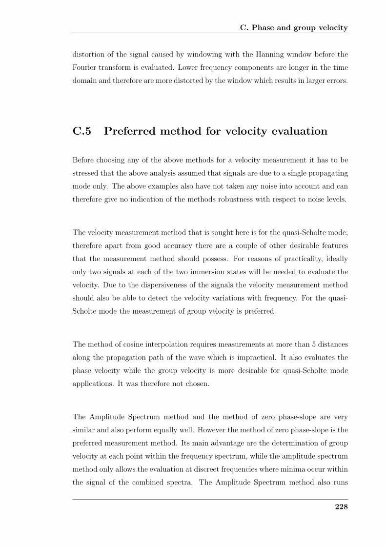
C. Phase and group velocity
distortion of the signal caused by windowing with the Hanning window before the
Fourier transform is evaluated. Lower frequency components are longer in the time
domain and therefore are more distorted by the window which results in larger errors.
C.5 Preferred method for velocity evaluation
Before choosing any of the above methods for a velocity measurement it has to be
stressed that the above analysis assumed that signals are due to a single propagating
mode only. The above examples also have not taken any noise into account and can
therefore give no indication of the methods robustness with respect to noise levels.
The velocity measurement method that is sought here is for the quasi-Scholte mode;
therefore apart from good accuracy there are a couple of other desirable features
that the measurement method should possess. For reasons of practicality, ideally
only two signals at each of the two immersion states will be needed to evaluate the
velocity. Due to the dispersiveness of the signals the velocity measurement method
should also be able to detect the velocity variations with frequency. For the quasi-
Scholte mode the measurement of group velocity is preferred.
The method of cosine interpolation requires measurements at more than 5 distances
along the propagation path of the wave which is impractical. It also evaluates the
phase velocity while the group velocity is more desirable for quasi-Scholte mode
applications. It was therefore not chosen.
The Amplitude Spectrum method and the method of zero phase-slope are very
similar and also perform equally well. However the method of zero phase-slope is the
preferred measurement method. Its main advantage are the determination of group
velocity at each point within the frequency spectrum, while the amplitude spectrum
method only allows the evaluation at discreet frequencies where minima occur within
the signal of the combined spectra. The Amplitude Spectrum method also runs
228

C. Phase and group velocity
into resolution problems when the term ΔF becomes small and of a comparable
magnitude to the frequency resolution of the spectrum (see section 4.7).
229

C. Phase and group velocity
C.6 Figures
Figure C.1: Phase(—) and group velocity (- - -) dispersion curve of the A0 mode of a
1mm thick steel plate (ρsteel = 7932kg/m3,Cl = 5959.5m/s, Cs = 3260m/s).
230
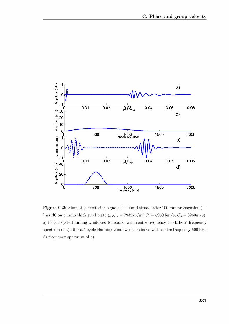
C. Phase and group velocity
Figure C.2: Simulated excitation signals (- - -) and signals after 100 mm propagation (—
) as A0 on a 1mm thick steel plate (ρsteel = 7932kg/m3,Cl = 5959.5m/s, Cs = 3260m/s).
a) for a 1 cycle Hanning windowed toneburst with centre frequency 500 kHz b) frequency
spectrum of a) c)for a 5 cycle Hanning windowed toneburst with centre frequency 500 kHz
d) frequency spectrum of c)
231
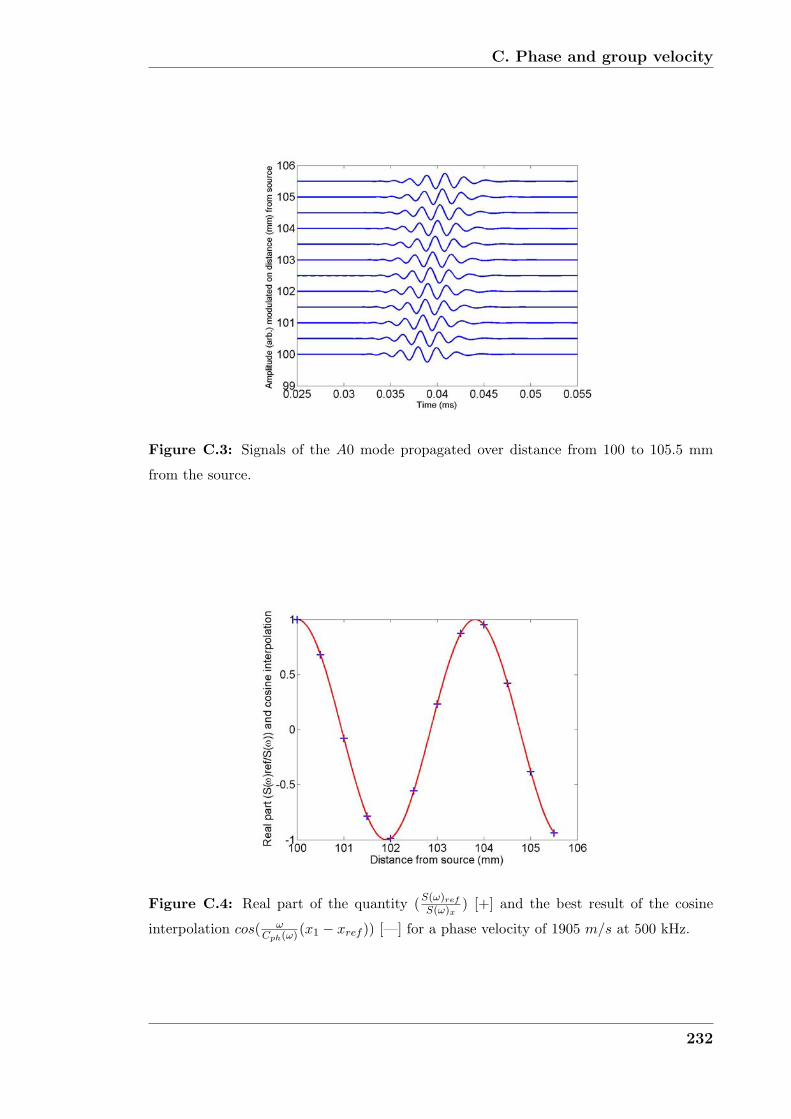
C. Phase and group velocity
Figure C.3: Signals of the A0 mode propagated over distance from 100 to 105.5 mm
from the source.
Figure C.4: Real part of the quantity (S(ω)ref
S(ω)x) [+] and the best result of the cosine
interpolation cos( ωCph(ω)(x1 − xref )) [—] for a phase velocity of 1905 m/s at 500 kHz.
232
C. Phase and group velocity
Figure C.5: A0 mode signals that were used to test the zero phase slope method for
group velocity measurement. Signal in a) has travelled for 100mm and signal in b) for
200mm as A0 mode in a 1mm thick steel plate.
233

C. Phase and group velocity
Figure C.6: Phase slope of both signals in figure C.5. [(- - -) signal a), (—) signal b)]
Figure C.7: Group velocity obtained using the zero phase slope method (- - -) and the
group velocity curve that was used to simulated the signals(—)
234
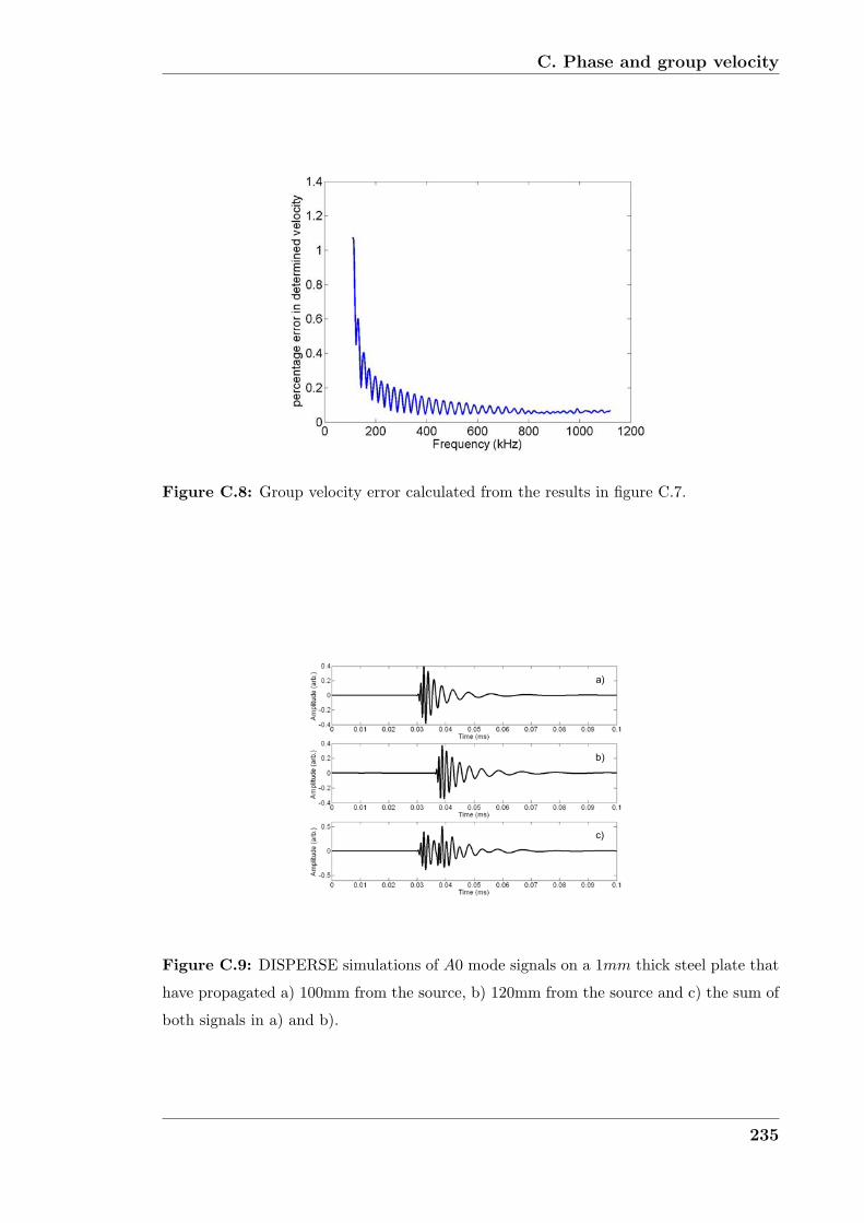
C. Phase and group velocity
Figure C.8: Group velocity error calculated from the results in figure C.7.
��
��
�
Figure C.9: DISPERSE simulations of A0 mode signals on a 1mm thick steel plate that
have propagated a) 100mm from the source, b) 120mm from the source and c) the sum of
both signals in a) and b).
235
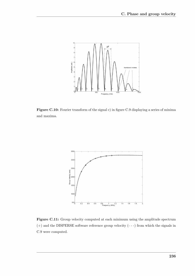
C. Phase and group velocity
Δ�
Figure C.10: Fourier transform of the signal c) in figure C.9 displaying a series of minima
and maxima.
Figure C.11: Group velocity computed at each minimum using the amplitude spectrum
(+) and the DISPERSE software reference group velocity (- - -) from which the signals in
C.9 were computed.
236
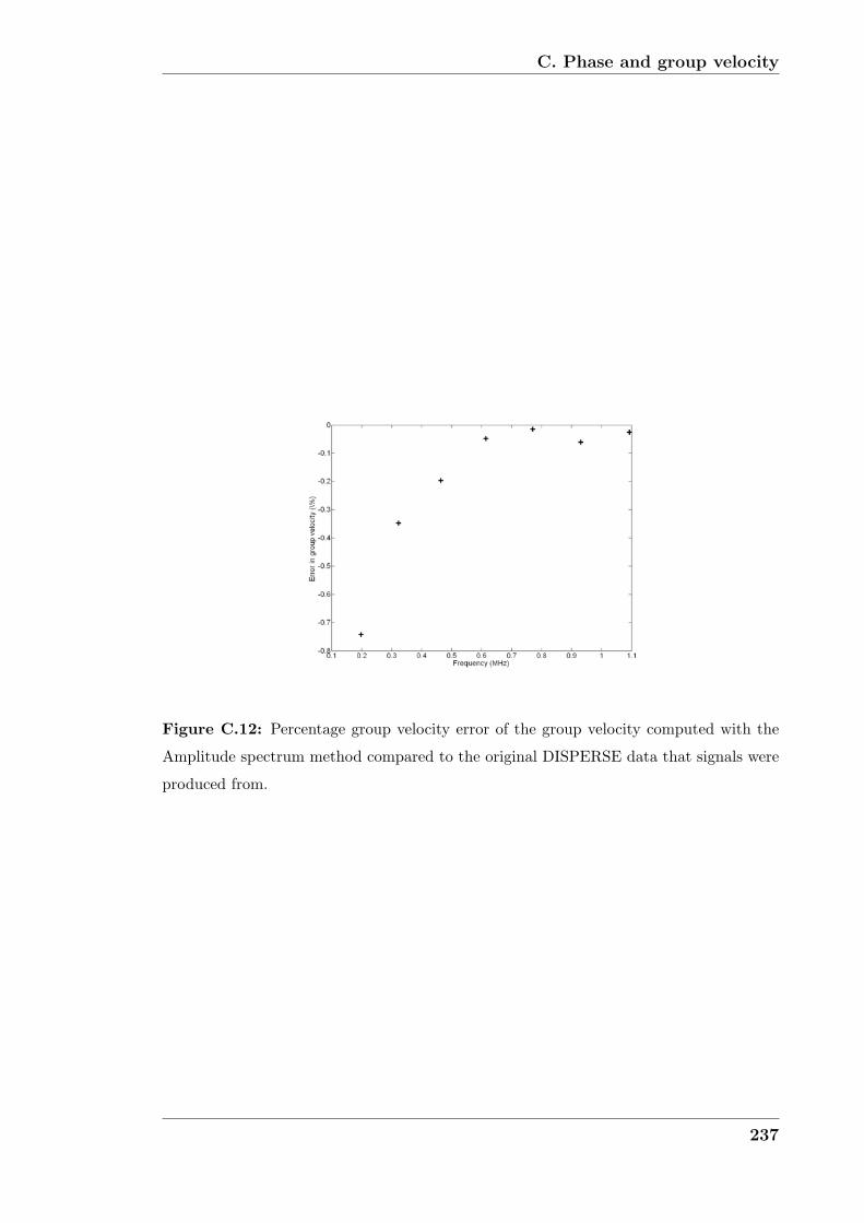
C. Phase and group velocity
Figure C.12: Percentage group velocity error of the group velocity computed with the
Amplitude spectrum method compared to the original DISPERSE data that signals were
produced from.
237
References
[1] M. J. W. Povey. Ultrasonic techniques for fluids characterization. Academic
Press, 1997.
[2] D.J. McClements. Advances in the application of ultrasound in food analysis
and processing. Trends in Food Sciences and Technology, 6, 1995.
[3] R. E. Challis, J. S. Tebbutt, and A. K. Holmes. Equivalence between three
scattering formulations for ultrasonic wave propagation in particluate mix-
tures. Journal of Physics D, 31:3481–3497, 1998.
[4] A. McNab, K.J. Kirk, and A. Cochran. Ultrasonic transducers for high tem-
perature applications. Science Measurement and Technology, IEE Proceedings,
145:229–236, 1998.
[5] N. Schmarje, J.F. Saillant, K.J. Kirk, and S. Cochran. Imaging with lithium
niobate/epoxy composites. Ultrasonics, 42:439–444, 2004.
[6] B. A. Auld. Acoustic fields and waves in solids I. Krieger Publishing Company,
1990.
[7] L.M. Brekhovskikh and V. Goncharov. Mechanics of continua and wave dy-
namics. Springer-Verlag, 1985.
[8] J. L. Rose. Ultrasonic Waves in Solid Media. Cambridge University Press,
1999.
[9] H. Kolsky. Stress waves in solids. Dover Publications, 1963.
[10] P. M. Morse and H. Feshbach. Methods of Theoretical Physics. McGraw-Hill
Book Company, 1953.
238
REFERENCES
[11] V.G. Mozhaev and M. Weihnacht. Subsonic leaky rayleigh waves at liquid-
solid interfaces. Ultrasonics, 40:927–933, 2002.
[12] N. Favretto-Anres. Theoretical study of the stoneley-scholte wave at the in-
terface between an ideal fluid and a viscoelastic solid. Acustica, 82:829 – 838,
1996.
[13] W. Fluegge. Viscoelasticity. Springer-Verlag, second edition, 1975.
[14] R.M. Christensen. Theory of Viscoelasticity. Academic Press, second edition,
1982.
[15] Y. M. Haddad. Viscoelasticity of engineering materials. Chapman and Hall,
1995.
[16] Lord Rayleigh. On waves propagating along the plane of an elastic solid.
Proceedings of the London Mathematical Society, 17:4–11, 1885.
[17] K. F. Graff. Wave Motion in Elastic Solids. Dover Publications, 1973.
[18] L.M. Brekhovskikh. Waves in layered media. Academic Press, 1980.
[19] H. Lamb. On waves in an elastic plate. In Conference of the Royal Society,
pages 114–128, London, 1917.
[20] D. Alleyne and P. Cawley. The long range detection of corrosion in pipes
using lamb waves. In D.O. Thompson and D.E. Chimenti, editors, Review of
Progress in Quantitative NDE, volume 14. Plenum Press, 1994.
[21] P. Wilcox, M. Lowe, and P. Cawley. Long range lamb wave inspection: The
effect of dispersion and modal selectivity. In D.O. Thompson and D.E. Chi-
menti, editors, Review of Progress in Quantitative NDE, volume 18. Plenum
Press, 1999.
[22] M.J.S. Lowe and B.N. Pavlakovic. Disperse user manual, version 2.0.11d. Tech-
nical report, Imperial College of Science, Technology and Medicine, London,
UK; www.ndt.imperial.ac.uk, 2001.
[23] M. Lowe. Matrix techniques for modelling ultrasonic waves in multilayered me-
dia. IEEE Transactions on Ultrasonics, Ferroelectrics and Frequency control,
42:525–542, 1995.
239
REFERENCES
[24] B. Pavlakovic, M. Lowe, D. Alleyne, and P. Cawley. Disperse: a general pur-
pose program for creating dispersion curves. In D.O. Thompson and D.E. Chi-
menti, editors, Review of Progress in Quantitative NDE, volume 16A. Plenum
Press, 1997.
[25] L. Knopoff. A matrix method for elastic wave problems. Bulletin of the
Seismological Society of America, 54:431–438, 1964.
[26] P.D. Wilcox. Lamb wave inspection of large structures using permanently at-
tached transducers. PhD thesis, Imperial College London, 1998.
[27] P. D. Wilcox, M. J. S. Lowe, and P. Cawley. A signal processing technique
to remove the effect of dispersion from guided wave signals. In D. O. Thomp-
son and D. E. Chimenti, editors, Review of Progress in Quantitative NDE,
volume 20. Plenum Press, 2001.
[28] P. Roux, B. Roman, and M. Fink. Time-reversal in an ultrasonic waveguide.
Applied Physics Letters, 70:1811–1813, 1997.
[29] M.G. Silk and K.F. Bainton. The propagation in metal tubing of ultrasonic
wave modes equivalent to lamb waves. Ultrasonics, 17:11–19, 1979.
[30] P. B. Nagy and R. M. Kent. Ultrasonic assessment of poisson’s ratio in thin
rods. Journal of the Acoustical Society of America, 98:269–2701, 1995.
[31] P.B. Nagy and A.H. Nayfeh. Viscosity-induced attenuation of longitudinal
guided waves in fluid-loaded rods. Journal of the Acoustical Society of Amer-
ica, 100:1501–1508, 1996.
[32] J. O. Kim and H. H. Bau. Online, real-time densimeter - theory and optim-
sation. Journal of the Acoustical Society of America, 85:432 – 439, 1989.
[33] C. L. Shepard and Friesel M. A. et al. Measurement of density and viscostiy
of one- and two-phase fluids with torsional waveguides. IEEE Transactions on
Ultrasonics, Ferroelectrics and Frequency control, 46:536–548, 1999.
[34] T. Vogt, M. Lowe, and P. Cawley. Cure monitoring using ultrasonic guided
waves in wires. Journal of the Acoustical Society of America, 114:1303–1313,
2003.
240

REFERENCES
[35] T.K. Vogt, J.S. Lowe, and P Cawley. Measurement of the material properties
of viscous liquids using ultrasonic guided waves. Ultrasonics, Ferroelectrics
and Frequency Control, IEEE Transactions on, 51:737–747, 2004.
[36] T. Vogt. Determination of Material Properties Using Guided Waves. PhD
thesis, Imperial College London, 2002.
[37] D.J. McClements. Principles of ultrasonic droplet size determination in emul-
sions. Langmuir, 12:3454–3461, 1996.
[38] A.K. Holmes and R.E. Challis. The applicability of acoustic wave propagation
models to silica sols and gels. Journal of Colloid and Interface Science, 216:50–
58, 1999.
[39] P.S. Epstein and R.R. Carhart. The absorption of sound in suspensions and
emulsions. i. water fog in air. Journal of the Acoustical Society of America,
25:553–565, 1953.
[40] J.R. Allegra and S.A. Hawley. Attenuation of sound in suspensions and emul-
sions: Theory and experiment. Journal of the Acoustical Society of America,
51:1545–1564, 1972.
[41] A.H. Harker and J.A. Temple. Velocity and attenuation of ultrasound in
suspensions of particles in fluids. Journal of Physics D, 21:1576–1588, 1988.
[42] A.N. Kalashnikov and R.E. Challis. Errors in the measurement of ultrasonic
absorption for materials evaluation. In D.O. Thompson and D.E. Chimenti,
editors, Review of Progress in Quantitative NDE, volume 21B, pages 1997–
2004. Plenum Press, 2002.
[43] P.C. Waterman and R.J. Truell. Multiple scattering of waves. Journal of
Mathematical Physics, 2:512–537, 1961.
[44] C. Glorieux, K. V. Rostyne, K. Nelson, W. Gao, W. Lauriks, and J. Thoen.
On the character of acoustic waves at the interface between hard and soft
solids and liquids. Journal of the Acoustical Society of America, 110:1299 –
1306, 2001.
241
REFERENCES
[45] J. G. Scholte. On the stoneley wave equation. In Geophysics, volume 45, pages
20–25. North Holland publishing, 1941.
[46] W.L. Pilant. Complex roots of the stonely wave equation. Bulletin of the
Seismological Society of America, 62:285–299, 1972.
[47] M. M. Vol’kenshtein and V. M. Levin. Structure of a stoneley wave at an
interface between a viscosus fluid and a solid. Soviet Physics - Acoustics,
34:351 – 355, 1987.
[48] F. Padilla, M. De Billy, and G. Quentin. Theoretical and experimental studies
of surface waves on solid-fluid interfaces when the value of the fluid sound
velocity is located between the shear and the longitudinal ones in the solid.
Journal of the Acoustical Society of America, 106:666 – 673, 1999.
[49] G. D. Meegan, M. F. Hamilton, Y. A. II’nskii, and E. A. Zabolotskaya. Nonlin-
ear stoneley and scholte waves. Journal of the Acoustical Society of America,
106:1712 – 1723, 1999.
[50] N. Favretto-Anres and G. Rabau. Excitation of the stoneley-scholte wave at
the boundary between an ideal fluid and a viscoelastic solid. Journal of Sound
and Vibration, 203:193 – 208, 1997.
[51] M. J. S. Lowe. Plate waves for the NDT of diffusion bonded titanium. PhD
thesis, Imperial College, 1992.
[52] T. Vogt, M. J. S. Lowe, and P. Cawley. Ultrasonic waveguide techniques
for the measurement of material properties. In D. O. Thompson and D. E.
Chimenti, editors, Review of Progress in Quantitative NDE, volume 21, pages
1 – 8. Plenum Press, 2002.
[53] F.B. Cegla, P. Cawley, and M.J.S. Lowe. Material property measurements
using the quasi-scholte mode - a waveguide sensor. Journal of the Acoustical
Society of America, 117:1098–1108, 2005.
[54] S. Nasr, J. Duclos, and M. Leduc. Pvdf transducers generating scholte waves.
Electronic Letters, 24:309 – 311, 1988.
242
REFERENCES
[55] J. McLean and F.L. Degertekin. Directional scholte wave generation and detec-
tion using interdigital capacitive micomachined ultrasonic transducers. IEEE
Transactions on Ultrasonics, Ferroelectrics and Frequency control, 51:756–64,
2004.
[56] C. Desmet, V. Gusev, W. Lauriks, C. Glorieux, and J. Thoen. Laser-induced
thermoelastic excitation of scholte wave. Applied Physics Letters, 68:2939 –
2941, 1996.
[57] M. De Billy and G. Quentin. Experimental study of the scholte wave propa-
gation on a plane surface partially immersed in a liquid. Journal of Applied
Physics, 54:4314–4322, 1983.
[58] T.J. Matula and P.L. Marston. Energy branching of a subsonic flexural wave
on a plate at an air-water interface. observation of the wave field near the
interface and near the plate. Journal of the Acoustical Society of America,
97:1389–1398, 1995.
[59] J. Dickey, G. Maidanik, and H. Ueberall. The splitting of dispersion curves for
the fluid-loaded plate. Journal of the Acoustical Society of America, 98:2365–
2367, 1995.
[60] T. Pialucha, C. C. H. Guyott, and P. Cawley. Amplitude spectrum method
for the measurement of phase velocity. Ultrasonics, 27:270–279, 1989.
[61] R. E. Challis, J. A. Harrison, A. K. Holmes, and R. P. Cocker. A wide band-
width spectrometer for rapid ultrasonic absorption measurements in liquids.
Journal of the Acoustical Society of America, 90:730–740, 1991.
[62] G.W.C. Kaye and T.H. Laby. Tables of physical and chemical constants. Long-
man, Harlow, 16 edition, 1995.
[63] A. Kulmyrzaev and D.J. McClements. High frequency dynamic shear rheology
of honey. Journal of Food Engineering, 45:219–224, 2000.
[64] R. S. C. Monkhouse, P. D. Wilcox, and P. Cawley. Flexible interdigital pvdf
transducers for the generation of lamb waves in structures. Ultrasonics, 35:489–
498, 1997.
243
REFERENCES
[65] A. M. Mills. Heat Transfer. Prentice-Hall, 1999.
[66] E. Papadakis, L.C. Lynnworth, K. A. Fowler, and E.H. Carnevale. Ultrasonic
attenuation and velocity in hot specimens by the momentary contact method
with pressure coupling, and some results on steel to 1200c. Journal of the
Acoustical Society of America, 52:850–857, 1972.
[67] W.N. Reynolds and R.L. Smith. Ultrasonic wave attenuation spectra in steels.
Journal of Applied Physics, 17:109–116, 1984.
[68] L.C. Lynnworth. Marginally dispersive ultrasonic waveguides, us patent
5,159,838, 1992.
[69] L.C. Lynnworth. Ultrasonic path bundle and systems, us patent 5,962,790,
1999.
[70] L.C. Lynnworth, L. Yi, and J.A. Umina. Extensional bundle waveguide tech-
niques for measuring flow of hot fluids. IEEE Transactions on Ultrasonics,
Ferroelectrics and Frequency control, 52:538–544, 2005.
[71] T.R. Winston and J.A. Brunk. Method and apparatus for ultrasonic inspection
of inaccessible areas, us patent 6,230,568, 2001.
[72] A.M. Heijnsdijk and J.M. van Klooster. Ultrasonic waveguide, us patent
6,400,648, 2002.
[73] C.K. Jen and J. G. Legoux. Clad ultrasonic waveguides with reduced trailing
echoes, us patent 5,828,274, 1998.
[74] C. K. Jen, J. W. Liaw, T. F. Chen, A. Moreau, J. P. Monchalin, and C. C.
Yang. Ultrasonic evaluation of semi-solid metals during processing. Measure-
ment Science & Technology, 11:1570–1575, 2000.
[75] A. U. Rehman, C. K. Jen, and I. Ihara. Ultrasonic probes for high temperature
immersion measurements. Measurement Science & Technology, 12:306–312,
2001.
[76] Y. Ono, Y. B. Zhang, C. K. Jen, J. F. Moisan, and C. Y. Su. Aluminum buffer
rods for ultrasonic monitoring at elevated temperatures. IEEE Transactions
on Ultrasonics Ferroelectrics and Frequency Control, 52:1042–1047, 2005.
244
REFERENCES
[77] H. Araki and Y. Matsunaga. Ultrasonic flow meter, us patent 4,014,211, 1977.
[78] A. Sather. Ultasonic buffer-rod technique for the high temperature measure-
ment of the elastic moduli of short specimens. Journal of the Acoustical Society
of America, 43:1291–1294, 1968.
[79] L.C. Lynnworth. Ultrasonic buffer/waveguide, us patent 6,047,602, 2000.
[80] R.D. Mindlin and E.A. Fox. Vibrations and waves in elastic bars of rectangular
cross section. Journal of Applied Mechanics, 27:152–158, 1960.
[81] P. Wilcox, M. Evans, O. Diligent, M. Lowe, and P. Cawley. Dispersion and
excitability of guided acoustic waves in isotropic beams with arbitrary cross
section. In D. O. Thompson and D. E. Chimenti, editors, Review of Progress
in Quantitative NDE, volume 20. Plenum Press, 2002.
[82] O. M. Mukdadi, Y. M. Desai, S. Datta, A. H. Shah, and A. J. Niklasson.
Elastic guided waves in a layered plate with rectangular cross section. Journal
of the Acoustical Society of America, 112:1766 – 1779, 2002.
[83] T. Hayashi, W. Song, and J.L. Rose. Guided wave dispersion curves for a bar
with an arbitrary cross-section, a rod and rail example. Ultrasonics, 41:175 –
183, 2003.
[84] L. Gavric. Computation of propagative waves in free rail using a finite element
technique. Journal of Sound and Vibration, 185:531–543, 1995.
[85] D. Hitchings. Fe77 user manual. Technical report, Imperial College of Science,
Technology and Medicine, London, UK, 1994.
[86] M. Drodz, L. Moreau, Castaings M., M.J.S. Lowe, and P. Cawley. Efficient
finite element modelling of absorbing regions for boundaries of guided wave
problems. In D. O. Thompson and D. E. Chimenti, editors, Review of Progress
in Quantitative NDE, 2005.
[87] N.C. Nicholson and W.N. McDicken. A comparison of coupling horns for
waveguides used in medical ultrasonics. Ultrasonics, 34:747–755, 1996.
245
REFERENCES
[88] S.K. Tang and C.K. Lau. Sound transmission across a smooth nonuniform
section in an infinitely long duct. Journal of the Acoustical Society of America,
112:2602–2611, 2002.
[89] D. Alleyne and P. Cawley. A two-dimensional fourier transform method for
the measurement of propagating multimode signals. Journal of the Acoustical
Society of America, 89:1159–1168, 1991.
[90] J.D. Achenbach. Wave propagation in elastic solids. North-Holland Publishing
Company, 1975.
[91] H. Lamb. On the propagation of tremors over the surface of an elastic solid.
Philosophical Transactions of the Royal Society of London. Series A, 203:1–42,
1904.
[92] G. F. Miller and H. Pursey. The field and radiation impedance of mechanical
radiators on the free surface of a semi-infinite isotropic solid. Proceedings of
the Royal Society, 223:521–541, 1954.
[93] G. F. Miller and H. Pursey. On the Partition of Energy between Elastic
Waves in a Semi-Infinite Solid. Royal Society of London Proceedings Series A,
233:55–69, December 1955.
[94] R.D. Woods. Screening of surface waves in soils. J. Soil Mech. Founds Div.
Am. Soc. civ. Engrs., July 94:951–79, 1968.
[95] P. Wilcox, R. Monkhouse, M. Lowe, and P. Cawley. The use of huygens’
principle to model the acoustic field from interdigital lamb wave transduc-
ers. In D. O. Thompson and D. E. Chimenti, editors, Review of progress in
quantitative NDE, 1998.
[96] J. D. N. Cheeke. Fundamentals and Applications of Ultrasonic waves. CRC
Press LLC, 2002.
[97] G. G. Stokes. Smith’s prize examination 1876. Mathematics and Physics
Papers (reprint), Cambridge University Press, 5:362, 1905.
[98] A. Bernard, M. J. S. Lowe, and M. Deschamps. Guided waves energy velocity
in absorbing and non-absorbing plates. Journal of the Acoustical Society of
America, 110:186 – 196, 2001.
246
REFERENCES
[99] W. Sachse and Y-H. Pao. On the determination of phase and group velocities
of dispersive waves in solids. Journal of Applied Physics, 49:4320–4327, 1978.
[100] F. Simonetti and Cawley P. A guided wave technique for the characterization
of highly attenuative viscoelastic materials. Journal of the Acoustical Society
of America, 114:158–165, 2003.
[101] P. B. Nagy. Personal communication: group velocity measurement using the
zero phase slope method, Nondestructive Evaluation Laboratory, Department
of Aerospace Engineering, University of Cincinnati, USA, 2005.
247

REFERENCES
Publications
Some of the material presented in this thesis has been published. The publication
details are listed below.
F.B. Cegla, P. Cawley, M.J.S. Lowe. Fluid characterisation using the Quasi-Scholte
mode. In D.O. Thompson and D.E. Chimenti, editors, Review of Progress in Quan-
titative NDE, Vol.24, pages 1584 − 1591, 2005
F.B. Cegla, P. Cawley, M.J.S. Lowe. Material property measurement using the
quasi-Scholte mode - A waveguide sensor. Journal of the Acoustical Society of Amer-
ica, Vol.117, Issue 3, pages 1098 − 1107, March 2005
F.B. Cegla, P. Cawley, M.J.S. Lowe. Measurement of bulk velocity and attenuation
in fluids and particle suspensions using the Quassi-Scholte mode. In D.O. Thomp-
son and D.E. Chimenti, editors, Review of Progress in Quantitative NDE, In press
2006
F.B. Cegla, P. Cawley, M.J.S. Lowe. Fluid bulk velocity and attenuation measure-
ments in non-Newtonian liquids using a dipstick sensor. Measurement Science and
Technology, Vol.17, Number 2, pages 264 − 274, February 2006
248