Embed Size (px)
Citation preview
IMPERIAL COLLEGE LONDON
Department of Earth Science and Engineering
Centre for Petroleum Studies
Modelling the Impact of Gas Cone Relaxation on Well Performance
By
Stephen Neil Buskie
In conjunction with BP
A report submitted in partial fulfillment of the requirements for the MSc and/or the
DIC.
September 2013


ii
Declaration of own Work
I declare that this thesis
“Modelling the Impact of Gas Cone Relaxation on Well Performance”
is entirely my own work and that where any material could be construed as the work of others, it is fully
cited and referenced, and/or with appropriate acknowledgement given.
Signature: ………………………………………………………………………..
Name of Student: Stephen Neil Buskie
Name of Academic supervisor: Professor Robert Zimmerman
Name of industry supervisors: David O’ Gorman, James Chesher, BP

iii
Abstract Gas coning during the production of oil is typically an unfavorable occurrence. This is because in-place gas helps maintain
reservoir pressure and drive oil production, while produced gas has a lower financial value than oil. For these reasons wells are
designed to minimise gas coning throughout the life of the field. In some instances however, gas production can be beneficial.
This study concentrates on the necessity for gas coning on certain wells that would typically be found within a brownfield
development.
This study applies steady-state nodal analysis to define the dependence some wells have on coning free gas for stable
production of oil. This study shows that a reduction in free gas can result in the cessation of production for these vulnerable
wells. Field data from Mirren, a BP operated oil field with an associated gas cap within the UKCS, which has shown a
dependence on free gas coning in the past, is used throughout this study.
Two-dimensional mechanistic numerical simulation analysis was coupled with the steady-state nodal analysis to
investigate the susceptibility to production losses incurred on well W150 due to gas cone relaxation during extended shut-in
periods. Pseudo oil-water and gas-oil relative permeability curves were created to reduce uncertainty through the inclusion of
field surveillance data and mitigate the impact of numerical dispersion within a coarse grid mechanistic model. An increase in
critical gas saturation from 3% to 7% is successful in capturing the results from fine scale simulations within a full-field scale
mechanistic model.
This analysis shows that relaxation of the gas cone during a ten day shut-in is sufficient to prevent the restart of production
on well W150. Although applying gas lift can provide sufficient lift to regain stable flow, it was noted that the oil rates are low
until the gas cone redevelops. The remedial action of bullheading gas into the reservoir after an extended shut-in period has
also been analysed within the mechanistic model. When compared to restarting the field using gas lift, bullheading resulted in
a 12% increase in cumulative oil production after restart, during a two week field ramp-up period.

iv
Acknowledgements
I would like to extend my gratitude towards David O’Gorman and James Chesher, along with the rest of the ETAP reservoir
management and base management teams at BP Aberdeen, for their guidance throughout this project. I would also like to
thank Professor Zimmerman for his direction during this research project.
v
Contents Declaration of own Work .............................................................................................................................................................. ii Abstract ........................................................................................................................................................................................ iii Acknowledgements ...................................................................................................................................................................... iv Contents ........................................................................................................................................................................................ v Table of Figures ........................................................................................................................................................................... vi Table of Tables ........................................................................................................................................................................... vii Abstract ......................................................................................................................................................................................... 1 Introduction ................................................................................................................................................................................... 1 Literature Review .......................................................................................................................................................................... 2 Analysis Tools .............................................................................................................................................................................. 3
Analytical Well Performance .............................................................................................................................................. 3 Steady State Nodal Analysis ............................................................................................................................................... 3 Pressure Transient Analysis ................................................................................................................................................ 3 Reservoir Simulation .......................................................................................................................................................... 4
Mirren Background Data: Field and Well Design Overview ........................................................................................................ 4 Well Design Overview.................................................................................................................................................... 5
Analysis, Results and Discussion .................................................................................................................................................. 5 Well Recovery Analysis ..................................................................................................................................................... 5 W150 Metastable Flow Analysis ........................................................................................................................................ 7 W150 Steady-State Well Performance ................................................................................................................................ 7 Mechanistic Modelling ....................................................................................................................................................... 9
History Matching. ........................................................................................................................................................... 9 Pressure Transient Analysis. ........................................................................................................................................... 9 Grid Comparison. ..........................................................................................................................................................11
Modelling and Results of Extended Shut-in Periods on Gas Cone Behaviour ..................................................................12 Remedial Options. .........................................................................................................................................................14
Further Discussion .......................................................................................................................................................................15 Further Work ................................................................................................................................................................................15 Conclusions ..................................................................................................................................................................................15 Acknowledgements ......................................................................................................................................................................16 Nomenclature ...............................................................................................................................................................................16 References ....................................................................................................................................................................................16 Appendices ...................................................................................................................................................................................17 Appendix A: Critical Literature Review on Modelling Gas Cone Behaviour ..............................................................................18 Appendix B: Framing Historical Well Performance ....................................................................................................................31 Appendix C: Steady-state Well Performance Setup .....................................................................................................................34 Appendix D: Mechanistic Model Quality Control and History Matching ...................................................................................39 Appendix E: Well Test Analysis Setup ........................................................................................................................................45 Appendix F: Material Balance Study ...........................................................................................................................................50 Appendix G: Further Gas Coning Analysis .................................................................................................................................54 Appendix H: Computer Software .................................................................................................................................................58
vi
Table of Figures Fig. 1: ETAP regional location within the North Sea, and the location of Mirren within ETAP. ................................................. 4 Fig. 2: Well placement and trajectory schematic. ......................................................................................................................... 5 Fig. 3: Historical shut-in and recovery times for W150, W151 and W152. Relaxation of the gas cone caused unstable flow on
wells W150 and W151 after two extended shut-in periods. .......................................................................................................... 6 Fig. 4: (a) Mirren shut-in time versus recovery time. (b) Flowing and shut-in wellhead pressures. ............................................. 6 Fig. 5: Well W150 daily average wellhead temperature, with no clear signs of metastable flow. ................................................ 7 Fig. 6: (a) VLP/IPR curves for W150 (PI=3.6, watercut=40%) showing the critical GOR for an intersection between the inflow
and outflow curves of 1560scf/bbl, and the subsequent increase in liquid rate for an increase in GOR to 4000scf/bbl. (b)
Sensitivity plot displaying the increase in critical GOR as watercut increases; Above 20% watercut well W150 requires
additional free gas above the solution GOR for a stable intersection between the inflow and outflow curves. ............................ 8 Fig. 7: (a) The impact productivity index has on the Critical GOR for W150, for watercuts between 0 and 70%. (b) Oil rate at
the critical GOR. ........................................................................................................................................................................... 8 Fig. 8: Fig. 8a Fine grid W150 mechanistic model with gas cone development at final timestep. Fig. 8b Coarse grid
mechanistic model with cone development at final timestep. Fine grid; 200:1:77 (DX:DY:DZ). Coarse grid; 20:1:9
(DX:DY:DZ). ................................................................................................................................................................................ 9 Fig. 9: Assessed pressure build-ups from well W152 in 2007, 2008 and 2012 and the corresponding pressure and derivative
response, including the simulated pressure match using the inclined well model. The overlay plot shows a clear decrease in
total mobility between the three tests. Pressure match and superposition plots for each build-up are available in Appendix E. 10 Fig. 10: (a) Original analog fractional flow and adapted Mirren fractional flow from well test analysis, showing that fractional
flow was conserved during the adaptation of oil-water relative permeability. (b) Original analog oil-water relative permeability
and total mobility rock curves, and the best fit Mirren well test analysis adapted oil-water relative permeability curves. .........10 Fig. 11: (a) Application of increased mobility from well test analysis during use in the mechanistic reservoir simulator. (b)
Highlights the influence the increased mobility has on the simulated bottom hole pressure as water breaks through. ...............11 Fig. 12: (a) Illustrates the affect the critical gas saturation increase has on the total mobility of the gas-oil phases. (b) Shows
the increase in critical gas saturation for each pseudo curve in more detail from the original analog value of 3%. ....................12 Fig. 13: (a) Simulation results of fine grid, coarse grid cumulative oil produced using original gas-oil relative permeability and
coarse grid using pseudo relative permeability curves (Sgcrit 0.07, 0.10 and 0.14). An increase in critical gas saturation from
3% to 7% provides the best match. (b) Percentage difference between coarse grid and fine grid simulation models with varying
Sgcrit. .............................................................................................................................................................................................12 Fig. 14: (a) Fine grid shut-in and recovery matrix, including gas lift rate and duration. (b) Equivalent coarse grid matrix. It is
clear that the coarse grid predicts more optimistic recovery times than the fine grid for the same gas lift usage and shut-in
duration. .......................................................................................................................................................................................13 Fig. 15: (a) Simulation recovery times compared to an uncertainty range given to well W150 observed data (from Fig. 4),
based on uncertainties from qualitative assessment of stable flow, and trend fitting bias towards the June 2012 shut-in. (b)
Relative GOR at restart of well W150 within the fine, coarse (with pseudo-curves) and coarse without critical gas saturation
modification. ................................................................................................................................................................................13 Fig. 16: Relative GOR contour maps for fine (left), coarse with 7% critical gas saturation (centre left) and coarse with original
gas-oil relative permeability curves (centre right). The pseudoisation has had a positive impact on capturing the gas cone
recovery between 20-100 days. Bullheading in the fine grid model lowers the risk that the GOR will drop by >60% for 0-40
day shut-ins (right). ......................................................................................................................................................................14 Fig. 17: (a) Impact on production rate and cumulative production during recovery for W150 after an extended shut-in period.
(b) Field ramp-up oil rate comparison after a 50day shut-in using 5days of gas lift on well W150 prior to gas lifting W152
(green series) or bullheading W150 for two days before providing gas lift to W152 (purple series). .........................................14
Appendix B Fig. 1: WHT displaying instabilities after the 2007 CATs export pipeline on Mirren well W151. .........................31 Appendix B Fig. 2: WHT displaying well performance instabilities after the 2012 extended shut-in period..............................31 Appendix B Fig. 3: W150 and W152 wellhead pressure behaviour during the 2012 shut-in period and recovery. ....................31 Appendix B Fig. 4: W150 daily average WHT. ...........................................................................................................................32 Appendix B Fig. 5: W152 daily average WHT ............................................................................................................................32 Appendix B Fig. 6: W151 daily average WHT ............................................................................................................................33
Appendix C Fig. 1: Well W150 VLP/IPR matched model based on measured production rates from March 2013. ..................35 Appendix C Fig. 2: Well W151 VLP/IPR matched model based on measured production rates from April 2010. ....................35 Appendix C Fig. 3: Well W152 VLP/IPR matched model based on measured production rates from March 2013. ..................36 Appendix C Fig. 4: Sensitivity of reservoir pressure on the critical GOR for well W150. ..........................................................36 Appendix C Fig. 5: Sensitivity of reservoir pressure on the stable oil production rate at the critical GOR for well W150. ........37 Appendix C Fig. 6: GOR, oil rate and PI sensitivity (40% watercut) ..........................................................................................38 Appendix C Fig. 7: GOR, oil rate and PI sensitivity (80% watercut) ..........................................................................................38
Appendix D Fig. 1: Reservoir pressure history match from fine and coarse grid mechanistic models. Achieved by scaling the

vii
production rates in-line with the in-place volumes of the mechanistic model. ............................................................................41 Appendix D Fig. 2: Well W150 oil rate and cumulative oil history match using fine grid. .........................................................41 Appendix D Fig. 3: Gas rate and cumulative gas history match using fine grid model. ..............................................................41 Appendix D Fig. 4: Water rate and cumulative water history match using fine grid model. .......................................................42 Appendix D Fig. 5: Oil rate and cumulative oil history matching using coarse grid model (Original gas-oil relative
permeability and pseudo relative permeability). ..........................................................................................................................42 Appendix D Fig. 6: Gas rate and cumulative gas history matching using coarse grid model (Original gas-oil relative
permeability and pseudo relative permeability). ..........................................................................................................................42 Appendix D Fig. 7: Water rate and cumulative water history matching using coarse grid model (Original gas-oil relative
permeability and pseudo relative permeability). ..........................................................................................................................43 Appendix D Fig. 8: GOR and watercut history match from fine and coarse grid (Sgcrit=7%) simulation models. ....................43 Appendix D Fig. 9: Simulated results matching the field observed recovery time based on an increase in W150 watercut from
42% to 83% to raise the critical GOR to 7500scf/bbl. .................................................................................................................44 Appendix D Fig. 10: Simulated effect of watercut on the recovery time after an extended shut-in period. ................................44
Appendix E Fig. 1: Mirren field reservoir pressure; Available downhole pressure data from all three Mirren wells corrected to
datum depth. .................................................................................................................................................................................45 Appendix E Fig. 2: Simulated model response based on radial flow stabilisation (2007: 0% Watercut) ....................................45 Appendix E Fig. 3: 2007 Pressure match using simulated model. ...............................................................................................46 Appendix E Fig. 4: 2007 Superposition match. ...........................................................................................................................46 Appendix E Fig. 5: Simulated model response based on radial flow stabilisation (2008: 15% Watercut) ..................................46 Appendix E Fig. 6: 2008 Pressure match using simulated model. ...............................................................................................47 Appendix E Fig. 7: 2008 Superposition match. ...........................................................................................................................47 Appendix E Fig. 8: Simulated model response based on radial flow stabilisation (2012: 54% Watercut) ..................................47 Appendix E Fig. 9: 2012 Pressure match using simulated model. ...............................................................................................48 Appendix E Fig. 10: 2012 Superposition match. .........................................................................................................................48
Appendix F Fig. 1: Three tank Mirren material balance representation.......................................................................................50 Appendix F Fig. 2: Six tank Mirren material balance representation. .........................................................................................51 Appendix F Fig. 3: Six tank Mirren material balance representation with additional aquifer support on well W150. ................52 Appendix F Fig. 4: Reservoir pressure estimation including wells W150, W151, W152, field average pressure and unproduced
southern volume. ..........................................................................................................................................................................53
Appendix G Fig. 1: Reservoir saturation within the fine and coarse grid mechanistic models, indicating the initial phase
distribution and the final phase distribution after production, with clear cone development. ......................................................54 Appendix G Fig. 2: Gas saturation surrounding near wellbore region of the fine grid mechanistic model during bullheading and
when producing with the support of gas lift after a 60day shut-in period. ...................................................................................55 Appendix G Fig. 3: Well W150 ramp-up rate after various shut-in periods, with and without bullheading................................56 Appendix G Fig. 4: Field ramp-up oil rate and cumulative oil produced after restart over a 2week ramp up period, after a
50day shut-in period.....................................................................................................................................................................57
Table of Tables Table 1: Available surveillance data on Mirren wells. “EH” denotes data available for “Entire History” of the well. ................ 3 Table 2: Summary of Mirren static rock and fluid properties. ...................................................................................................... 5 Table 3: Well Design Summary. ................................................................................................................................................... 5 Table 4: Well test analysis parameter results. ..............................................................................................................................10 Table 5: Comparison between fine and coarse grid simulation model cumulative produced volumes. .......................................12 Table 6: Recommended Mirren start-up procedure (Summarised from Appendix G Table 1) ....................................................16 Appendix C Table 1: Well W150 completion input for use within the steady-state nodal analysis package. .............................34 Appendix C Table 2: Mirren PVT used within all well performance analysis. ...........................................................................34 Appendix C Table 3: Calculated and measured production rates and bottom hole pressure from well W150. ...........................35 Appendix D Table 1: Mirren Black Oil PVT data used within numerical reservoir simulation model. ......................................40 Appendix D Table 2: Mirren water properties. ............................................................................................................................40 Appendix D Table 3: Grid volumetric quality control .................................................................................................................40 Appendix E Table 1: Well test analysis parameter results. ..........................................................................................................49 Appendix E Table 2: Results from iterative method to calculate water saturations and relative permeabilities based on the
watercut and normalised mobility thickness observed during well test analysis. ........................................................................49 Appendix G Table 1:Recommended start-up procedure based mechanistic reservoir simulation analyses and relative GOR
contour maps. ...............................................................................................................................................................................57

viii
Page intentionally left blank.

Imperial College
London Candidate Paper Modelling the Impact of Gas Cone Relaxation on Well Performance Stephen Buskie
Imperial College supervisor: Professor Robert Zimmerman Industry supervisor: David O’Gorman, James Chesher, BP., Aberdeen This paper was prepared for partial fulfillment of MSc in Petroleum Engineering, Imperial College London, 27 September 2013.
Abstract Gas coning during the production of oil is typically an unfavorable occurrence. This is because in-place gas helps maintain
reservoir pressure and drive oil production, while produced gas has a lower financial value than oil. For these reasons wells are
designed to minimise gas coning throughout the life of the field. In some instances however, gas production can be beneficial.
This study concentrates on the necessity for gas coning on certain wells that would typically be found within a brownfield
development.
This study applies steady-state nodal analysis to define the dependence some wells have on coning free gas for stable
production of oil. This study shows that a reduction in free gas can result in the cessation of production for these vulnerable
wells. Field data from Mirren, a BP operated oil field with an associated gas cap within the UKCS, which has shown a
dependence on free gas coning in the past, is used throughout this study.
Two-dimensional mechanistic numerical simulation analysis was coupled with the steady-state nodal analysis to
investigate the susceptibility to production losses incurred on well W150 due to gas cone relaxation during extended shut-in
periods. Pseudo oil-water and gas-oil relative permeability curves were created to reduce uncertainty through the inclusion of
field surveillance data and mitigate the impact of numerical dispersion within a coarse grid mechanistic model. An increase in
critical gas saturation from 3% to 7% is successful in capturing the results from fine scale simulations within a full-field scale
mechanistic model.
This analysis shows that relaxation of the gas cone during a ten day shut-in is sufficient to prevent the restart of production
on well W150. Although applying gas lift can provide sufficient lift to regain stable flow, it was noted that the oil rates are low
until the gas cone redevelops. The remedial action of bullheading gas into the reservoir after an extended shut-in period has
also been analysed within the mechanistic model. When compared to restarting the field using gas lift, bullheading resulted in
a 12% increase in cumulative oil production after restart, during a two week field ramp-up period.
Introduction Gas coning is a frequently occurring and well-studied phenomenon that develops during the production of oil from a saturated
oil field with associated free gas. In such reservoirs, oil and gas are initially segregated due to fluid density contrasts. When
static equilibrium is achieved between these two fluid phases, the flow of oil can occur in the oil zone without the additional
flow of gas. If the pressure gradient at the near-well region exceeds the force balance between the fluids (either oil and gas for
gas coning, or equally, oil and water for water coning) then coning can occur (Muskat and Wyckoff, 1935). Gas coning is
typically described as an unattractive result of oil production from a field with an associated gas cap. This is because the
economic value of gas is lower than oil, while gas also maintains pressure within a reservoir during depletion. Multiphase
production of oil and gas also reduces the mobility of oil and lowers the production rates (Dake, 1978). Equally, water coning
is unattractive; not only does water production increase the operating cost of hydrocarbon extraction due to the expense of
water disposal, but many mature fields are nearing or operating at production constraints due to limited availability of
produced water disposal facilities. For these reasons wells are designed to delay the breakthrough of water or gas. However,
although rarely discussed, gas coning can provide positive benefits towards the recovery of hydrocarbons from a reservoir,
under certain conditions.
These conditions include substantial reservoir pressure depletion, mid-high watercuts and poor artificial lift availability.
For a reservoir that is producing under such conditions there is a genuine risk that the loss of the gas cone can have severe
consequences on the ultimate recovery of the field. The relaxation or ultimate loss of a gas cone would be triggered by a
cessation of production. Without the pressure drawdown towards a producing well the buoyancy forces will become dominant
and gas will migrate upwards due to its density difference with oil and water (Meyer, 1954). This paper will look at the
susceptibility to production losses due to gas cone relaxation incurred through extended shut-in periods. The study uses
production data from Mirren, a BP operated field that fits the above criterion for a field that may be susceptible to gas cone
relaxation production losses.
The primary aim of this study is focused on the assessment of well performance on well 22/25B-7 (W150) within Mirren,
and how this is linked to gas coning. The behaviour of gas cone relaxation is captured through the use of mechanistic
numerical simulation models and coupled to the well performance using steady-state nodal analysis. A secondary aim of the
study investigates the specific alterations required to model the behaviour of gas cone relaxation within a fine and coarse grid
simulation model that matches the observed production data from the Mirren field. This includes calibration of oil-water
relative permeability data based on well test analysis and the pseudoisation of gas-oil relative permeability curves in an
upscaling process to limit the impact of numerical dispersion that occurs within a coarse grid mechanistic model. The results
2 S. Buskie Candidate Paper
provided by a coarse grid simulation model are of significant importance since production forecasts are based upon the
predictions from coarse grid full-field reservoir simulation models. This study shows that such predictions can be optimistic
for wells that are susceptible to production losses after extended shut-in periods.
Remedial options are discussed for cases when production cannot be regained due to severe gas cone relaxation. Predictive
reservoir simulation cases are ran to model the effects of bullheading, the most favorable remedy.
The findings will illustrate the positive benefits that gas coning can provide to an aging well, while also providing
recommendations to aid operational decisions for the Mirren field. The products of modified oil-water and pseudo gas-oil
relative permeability curves from this study will also contribute to future dynamic simulation work on the Mirren field.
Finally, this study provides a workflow for future analysis of at-risk wells on analog fields within the BP portfolio.
Literature Review Investigations into gas coning have been on-going since 1935 when Muskat and Wyckoff first described an approximate
theory of water coning during oil production from a vertical well (Muskat and Wyckoff, 1935). The analysis set about
describing an equilibrium condition that allows the production of oil without the coning of water, based on the pressure drop
that is created between the reservoir outer boundaries and the well perforation. A type curve displaying the critical pressure
differential required to develop a cone was presented, which also included the effect of oil zone thickness and well penetration.
For practical reasons this was modified to bring together the relationship between oil production rate and pressure difference.
Similarly, Meyer and Garder (Meyer, 1954) assessed the production of oil or gas from a reservoir with an underlying water
table, the production of oil with an overlying gas cap and the production of oil from a reservoir with an overlying gas cap and
underlying water table, all with the aim of determining the maximum allowable oil production rate without the coning of either
water, gas or both water and gas for the applicable cases. These two papers analytically describe the mechanism of coning and
seek a means of limiting it. This set the trend for future discussions related to both water and gas coning.
The next major step in the analysis of coning was brought about by Weber and Welge. They realised that the dynamics of
water or gas coning were well suited to two-dimensional gridded calculations and so used the alternating direction implicit
method, a computational calculation procedure, to model gas and water coning (Welge and Weber, 1964). The importance of
fine grid blocks in the near wellbore region was highlighted. The two-dimensional model was then used to predict the results
obtained from earlier laboratory experiments. Good matches between computed and experimental water breakthrough times
were provided which validated the applicability of the two-dimensional coning model. Soon after, Sobocinski and Cornelius
generated a correlation for dimensionless cone height against dimensionless time and confirmed their results using a computer
simulation model (Sobocinski and Cornelius, 1965). They also highlighted the strength of simulation models to assess the
impact of specific complexities, such as reservoir heterogeneities, which are difficult to capture in a general analytical
solution. Since this study, many others have proven the potential for simulation models to accurately capture the behavior of
reservoir dynamics. For instance, reservoir simulation is classified as an analytical procedure which may be used during the
estimation of recoverable hydrocarbon reserves due to its contribution to the field of reservoir engineering over the years
(SPE/AAPG/WPC/SPEE, 2007).
From the early days of reservoir simulations the users have tried to increase computational efficiency while maintaining
accuracy and an acceptable level of error. Simplification of a model is the most common technique to ensure analysis runtime
is not excessive. This is usually achieved by reducing the number of grid blocks that define the model. However, as was noted
in the first two-dimensional analysis of coning, small or “fine” grid blocks are beneficial for capturing the near wellbore
behavior of gas or water coning (Welge and Weber, 1964). As such, the next logical step in modelling the behavior of coning
was to investigate workaround procedures to gain similar results found using a computationally expensive fine grid model
using a coarser model. Woods and Khurana noted that the large grid cells in a full field model mask the effects of coning
(Woods and Khurana, 1977). The skew of results obtained on a coarse grid model when compared to a fine scale model is
termed numerical dispersion. Numerical dispersion is a product of the discretization of the reservoir model. Grid blocks are
homogeneous volumes with a uniform saturation and pressure at each time step. Within a coarse model there is a greater
amount of averaging of these pressure and saturation values, which results in a loss of definition and increases the effects of
numerical dispersion.
Numerical dispersion is particularly important in studies of water flooding, gas flooding or coning. This is because the
calculation of mobility of fluids within a reservoir simulator is made at the interface between cells. However, since only cell
centres are calculation nodes the simulation assigns the mobility at the face to be equal to the computed value at the cell centre
of the upstream, higher potential, grid block (Jr et al., 1979). This can result in earlier breakthrough times than those observed
in reality. To overcome the effects of numerical dispersion while modelling water coning, Woods and Khurana (1979) created
pseudofunctions to capture water coning behavior in a three-dimensional reservoir simulator. The proposed solution was to
mathematically adapt the well performance results from a detailed well-coning model into pseudo relative permeability and
capillary-pressure curves which could then be applied in a reservoir model. Their adaptations provided good matches between
the fine and coarse grid models. An alternative means to capture gas coning behavior in large grid block models through the
application of coning correlations was purposed by Addington (1981). The coning correlations were successfully applied to a
five-layer large grid cell model. These two studies show that the effects of numerical dispersion can be corrected successfully
during coning studies.
As noted earlier, all published literature focus on the critical oil production rate to minimize coning and therefore maximize
the production of oil. This may be the most sensible development option, and certainly would be in a field with wells that
perform strongly throughout the entire field life, either due to efficient artificial lift methods, or a maintained reservoir
Candidate Paper Modelling the Impact of Gas Cone Relaxation on Well Performance 3
pressure. However, for reservoirs on primary depletion with no pressure support, like Mirren, the absolute open flow potential
of each well declines with the reservoir pressure. The positive benefits that gas coning can provide to such wells have not been
clearly documented. This paper will assess such benefits, while also investigating the susceptibility to production losses that
could be incurred due to a relaxation of the gas cone during an extended shut-in period.
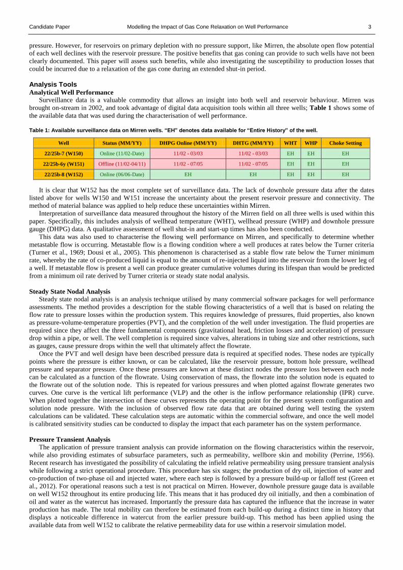
Analysis Tools Analytical Well Performance
Surveillance data is a valuable commodity that allows an insight into both well and reservoir behaviour. Mirren was
brought on-stream in 2002, and took advantage of digital data acquisition tools within all three wells; Table 1 shows some of
the available data that was used during the characterisation of well performance.
Table 1: Available surveillance data on Mirren wells. “EH” denotes data available for “Entire History” of the well.
Well Status (MM/YY) DHPG Online (MM/YY) DHTG (MM/YY) WHT WHP Choke Setting
22/25b-7 (W150) Online (11/02-Date) 11/02 - 03/03 11/02 - 03/03 EH EH EH
22/25b-6y (W151) Offline (11/02-04/11) 11/02 - 07/05 11/02 - 07/05 EH EH EH
22/25b-8 (W152) Online (06/06-Date) EH EH EH EH EH
It is clear that W152 has the most complete set of surveillance data. The lack of downhole pressure data after the dates
listed above for wells W150 and W151 increase the uncertainty about the present reservoir pressure and connectivity. The
method of material balance was applied to help reduce these uncertainties within Mirren.
Interpretation of surveillance data measured throughout the history of the Mirren field on all three wells is used within this
paper. Specifically, this includes analysis of wellhead temperature (WHT), wellhead pressure (WHP) and downhole pressure
gauge (DHPG) data. A qualitative assessment of well shut-in and start-up times has also been conducted.
This data was also used to characterise the flowing well performance on Mirren, and specifically to determine whether
metastable flow is occurring. Metastable flow is a flowing condition where a well produces at rates below the Turner criteria
(Turner et al., 1969; Dousi et al., 2005). This phenomenon is characterised as a stable flow rate below the Turner minimum
rate, whereby the rate of co-produced liquid is equal to the amount of re-injected liquid into the reservoir from the lower leg of
a well. If metastable flow is present a well can produce greater cumulative volumes during its lifespan than would be predicted
from a minimum oil rate derived by Turner criteria or steady state nodal analysis.
Steady State Nodal Analysis
Steady state nodal analysis is an analysis technique utilised by many commercial software packages for well performance
assessments. The method provides a description for the stable flowing characteristics of a well that is based on relating the
flow rate to pressure losses within the production system. This requires knowledge of pressures, fluid properties, also known
as pressure-volume-temperature properties (PVT), and the completion of the well under investigation. The fluid properties are
required since they affect the three fundamental components (gravitational head, friction losses and acceleration) of pressure
drop within a pipe, or well. The well completion is required since valves, alterations in tubing size and other restrictions, such
as gauges, cause pressure drops within the well that ultimately affect the flowrate.
Once the PVT and well design have been described pressure data is required at specified nodes. These nodes are typically
points where the pressure is either known, or can be calculated, like the reservoir pressure, bottom hole pressure, wellhead
pressure and separator pressure. Once these pressures are known at these distinct nodes the pressure loss between each node
can be calculated as a function of the flowrate. Using conservation of mass, the flowrate into the solution node is equated to
the flowrate out of the solution node. This is repeated for various pressures and when plotted against flowrate generates two
curves. One curve is the vertical lift performance (VLP) and the other is the inflow performance relationship (IPR) curve.
When plotted together the intersection of these curves represents the operating point for the present system configuration and
solution node pressure. With the inclusion of observed flow rate data that are obtained during well testing the system
calculations can be validated. These calculation steps are automatic within the commercial software, and once the well model
is calibrated sensitivity studies can be conducted to display the impact that each parameter has on the system performance.
Pressure Transient Analysis
The application of pressure transient analysis can provide information on the flowing characteristics within the reservoir,
while also providing estimates of subsurface parameters, such as permeability, wellbore skin and mobility (Perrine, 1956).
Recent research has investigated the possibility of calculating the infield relative permeability using pressure transient analysis
while following a strict operational procedure. This procedure has six stages; the production of dry oil, injection of water and
co-production of two-phase oil and injected water, where each step is followed by a pressure build-up or falloff test (Green et
al., 2012). For operational reasons such a test is not practical on Mirren. However, downhole pressure gauge data is available
on well W152 throughout its entire producing life. This means that it has produced dry oil initially, and then a combination of
oil and water as the watercut has increased. Importantly the pressure data has captured the influence that the increase in water
production has made. The total mobility can therefore be estimated from each build-up during a distinct time in history that
displays a noticeable difference in watercut from the earlier pressure build-up. This method has been applied using the
available data from well W152 to calibrate the relative permeability data for use within a reservoir simulation model.
4 S. Buskie Candidate Paper
Reservoir Simulation
Analysis of the dynamic fluid behaviour within a reservoir simulation model is conducted using a commercially available
software package. This requires the creation of a geological grid at a specified depth to define the bulk rock volume of the
model. This is then converted into a pore volume by the inclusion of porosity and net to gross. With the input of more rock
properties, most notably compressibility, permeability, relative permeability and capillary pressure data the model is ready for
setup of the initial conditions. The initial conditions include the reservoir temperature, pressure and fluids distribution.
Once initialisation is complete, which will result in a propagation of fluid saturations within the model, calibration of the
model can commence. Dynamic simulation model calibration is based on matching the simulated performance to observed
field production data, often termed calibration data. This process is known as history matching. Once history matching is
complete, and an acceptable match between simulated performance and observed data has been made the simulation model has
been validated, and can be used for future performance prediction. This process has been followed during the mechanistic
reservoir simulation study of well W150 performance.
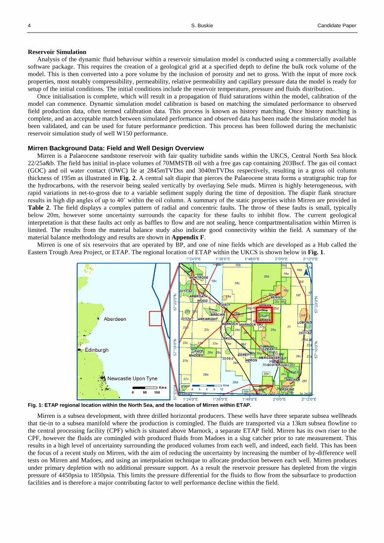
Mirren Background Data: Field and Well Design Overview Mirren is a Palaeocene sandstone reservoir with fair quality turbidite sands within the UKCS, Central North Sea block
22/25a&b. The field has initial in-place volumes of 70MMSTB oil with a free gas cap containing 203Bscf. The gas oil contact
(GOC) and oil water contact (OWC) lie at 2845mTVDss and 3040mTVDss respectively, resulting in a gross oil column
thickness of 195m as illustrated in Fig. 2. A central salt diapir that pierces the Palaeocene strata forms a stratigraphic trap for
the hydrocarbons, with the reservoir being sealed vertically by overlaying Sele muds. Mirren is highly heterogeneous, with
rapid variations in net-to-gross due to a variable sediment supply during the time of deposition. The diapir flank structure
results in high dip angles of up to 40˚ within the oil column. A summary of the static properties within Mirren are provided in
Table 2. The field displays a complex pattern of radial and concentric faults. The throw of these faults is small, typically
below 20m, however some uncertainty surrounds the capacity for these faults to inhibit flow. The current geological
interpretation is that these faults act only as baffles to flow and are not sealing, hence compartmentalisation within Mirren is
limited. The results from the material balance study also indicate good connectivity within the field. A summary of the
material balance methodology and results are shown in Appendix F.
Mirren is one of six reservoirs that are operated by BP, and one of nine fields which are developed as a Hub called the
Eastern Trough Area Project, or ETAP. The regional location of ETAP within the UKCS is shown below in Fig. 1.
Fig. 1: ETAP regional location within the North Sea, and the location of Mirren within ETAP.
Mirren is a subsea development, with three drilled horizontal producers. These wells have three separate subsea wellheads
that tie-in to a subsea manifold where the production is comingled. The fluids are transported via a 13km subsea flowline to
the central processing facility (CPF) which is situated above Marnock, a separate ETAP field. Mirren has its own riser to the
CPF, however the fluids are comingled with produced fluids from Madoes in a slug catcher prior to rate measurement. This
results in a high level of uncertainty surrounding the produced volumes from each well, and indeed, each field. This has been
the focus of a recent study on Mirren, with the aim of reducing the uncertainty by increasing the number of by-difference well
tests on Mirren and Madoes, and using an interpolation technique to allocate production between each well. Mirren produces
under primary depletion with no additional pressure support. As a result the reservoir pressure has depleted from the virgin
pressure of 4450psia to 1850psia. This limits the pressure differential for the fluids to flow from the subsurface to production
facilities and is therefore a major contributing factor to well performance decline within the field.

Candidate Paper Modelling the Impact of Gas Cone Relaxation on Well Performance 5
Well Design Overview. The three wells on Mirren, W150, W151 and W152 have similar designs in general. They are
horizontal linear chord trajectories across the reservoir ‘doughnut’ that surrounds the salt diapir. This was to dissect the
reservoir stratiographic section twice, tangential to the base reservoir Chalk in the trajectory mid-point. This militates against
fault compartmentalisation. The chalk does not contribute to any hydrocarbon production, and only the sandstone is perforated.
Some key well design parameters are listed in Table 3. Table 2: Summary of Mirren static rock and fluid properties.
Fig. 2: Well placement and trajectory schematic.
Table 3: Well Design Summary.
Well Depth
(m TVDss)
Perforation Length
(m) Standoff to GOC (m) Standoff to OWC (m)
Gas lift Mandrel Depth
(m TVDss)
Initial PI
(bbl/day/psi)
W150 2938 613 93 102 2663.6 12
W151 2934 443 89 106 2702.7 9
W152 2970 449 125 70 1867, 2781 4
Gas lift is available on all three wells. Gas is delivered to the gas lift system via a subsea umbilical. This is rate constrained
to roughly 2.0MMscf/d, due to the small diameter 1” delivery line within the subsea umbilical. Gas lift can only be applied to
one well at a time on Mirren, and is presently used to start-up each well. The gas lift is controlled using an annular wing value
within the wells. The gas lift design on well W152 is more efficient than the older wells W150 and W151. Firstly, there are
two gas lift mandrels within W152. During start-up the shallow mandrel operates first to unload the upper section of the well.
This valve then closes and the gas is bypassed and injected through the lower mandrel, unloading the lower section of the well.
Wells W150 and W151 only have one injection point, meaning the same gas volume has to unload a larger column of liquid.
Secondly, the depth of injection is 78m deeper with respect to the mid-perforation depth on well W152 than the other two
wells. This means that in two stages the gas is able to aerate a larger volume of liquid within W152. The limitations on gas lift
rate and the depth of injection on wells W150 and W151 are considered to be contributors to the well performance instabilities
that are experienced after extended shut-in periods.
The present start-up procedure for Mirren is as follows. Well W152 start-up is initiated first, with full gas lift, with a target
of 100% choke. Once well W152 is flowing stably, and no longer needs gas lift, the supply of gas can be directed to well
W150. The target for well W150 is also 100% choke. Well W151 is presently offline since its death in 2011. Restart attempts
are not made due to technical issues within the subsea flexible flowline.
Analysis, Results and Discussion Well Recovery Analysis
A qualitative assessment of the recovery time of each well after a shut-in period was conducted. The recovery time is the time
it takes between the well opening to flow and reaching the pre-shut-in flowing conditions. This is to characterise the
differences between the recovery times of these wells. More specifically stable production was characterised by: a return to
pre-shut-in flowing WHT, a return to pre-shut-in flowing WHP and the cessation of gas lift. More detail on the
characterisation of stable flow, including WHT and WHP trends are provided in Appendix B.
These criteria for quantifying stable flow introduce some error in the comparison between these wells. For instance, the
chokes may be opened and closed during a single restart procedure for operational reasons. This affects the pressure
Oil Gravity (°API) 41 Rock Type Sandstone
Gas Gravity (S.G) (air = 1) 0.79 Stratigraphic UnitsLista, Forties,
Maureen
Solution Gas Oil Ratio (scf/bbl) 1285 Trap Type Salt Diapir
Bubble Point Pressure (psia) 4576Reservoir Thickness
(m)195
Virgin Reservoir Pressure
(psia)4557
Rock Compressibility
(1/psi)4x10
-6
Current Reservoir Pressure
(2013) (psia)1854
Porosity Range
(fraction)0.15-0.22
At datum depth (mTVDss) 2845Permeability Range
(mD)0.1-100
Reservoir Temperature (°f) 235 Net-to-Gross (ratio) 0.3-0.5
Mirren Static Reservoir Properties
Fluid Properties Rock Properties

6 S. Buskie Candidate Paper
distribution within the reservoir, and will alter the recovery process. The influence of this is cannot be captured by this
qualitative assessment. Equally, gas lift may be applied and removed many times during one recovery attempt, since there is a
minimum temperature constraint within the flowline and prolonged gas lift use introduces the risk that this temperature limit
will be exceeded. This again has an effect on the wells recovery to the pre-shut-in conditions. The behaviour of the WHT and
WHP after a prolonged shut-in period is illustrated in Appendix B Fig. 1-3.
A second limitation of this analysis is that it is independent of the date at which the shut-in took place. While comparing
recovery time throughout the entire history of a well, there is likely to be a natural decline in well performance, caused by a
decline in reservoir pressure or increase in watercut for instance.
Fig. 3: Historical shut-in and recovery times for W150, W151 and W152. Relaxation of the gas cone caused unstable flow on wells W150 and W151 after two extended shut-in periods.
Fig. 4: (a) Mirren shut-in time versus recovery time. (b) Flowing and shut-in wellhead pressures.
0
10
20
30
40
50
60
70
1 10 100
Re
cove
ry D
ura
tio
n (
Day
s)
Shut-in Duration (Days)
W150 W151 W152
0
500
1000
1500
2000
2500
06/06/2006 05/06/2008 06/06/2010 05/06/2012
WH
P, F
low
ing
and
Sh
ut-
in (
psi
a)
W151 WHP flowing W151 WHP shut in W152 WHP flowingW152 WHP shut in W150 WHP flowing W150 WHP shut in
Candidate Paper Modelling the Impact of Gas Cone Relaxation on Well Performance 7
From the data shown in Fig. 3, a semi-logarithmic scatter plot of shut-in duration versus recovery times was created (Fig.
4a). The flowing WHP and shut-in WHP for each shut-in period was also recorded (Fig. 4b).
A logarithmic regression line provides the best fit through the observed data, however, for the case of W150 the trend is
biased towards the second most recent shut-in period. This data point is an outlier; before this shut-in the recovery time for
W150 fell on a similar trend to W152. The outcome of this is that the observed trend for W150 may overestimate the recovery
time in the future. Analysis of this sort cannot be relied upon to present accurate results for future predictions. For this reason a
mechanistic study of the reservoir is required. The mechanistic model will capture the dynamic effect within the reservoir
during an extended shut-in period. The results will be compared with the above analysis as a means of verification.
Fig. 4b shows a difference of 500psi between the shut-in WHP of W150 and W152 by the start of 2012. Assuming a
homogeneous reservoir pressure, as is done during all analyses on Mirren, an increased shut-in wellhead pressure indicates a
smaller pressure drop within the wellbore. This would be caused by a lower average fluid density within W150. During the
most recent by-difference well test on 18/03/2013, W152 produced with a watercut of 60% and a gas-oil ration (GOR) of
9800scf/bbl, while W150 produced with a lower watercut of 42% and a marginally higher GOR of 9900scf/d. Since W150 has
a lower watercut and higher GOR than well W152, the reduced flowing WHP is logical.
W150 Metastable Flow Analysis
A check for the presence of metastable flow on the wells on Mirren was conducted, following the method outlined by
Dousi et al (2005). WHT is a direct indication of fluid production from a well. When metastable flow is present the measured
WHT is below the WHT observed during stable flow, since metastable flow rates are lower than stable flow rates. This can be
observed in measured WHT data by plotting a daily average WHT over the course of a year. The stable flowing WHT and
shut-in periods will be clearly visible as an elevated temperature and ambient WHT respectively. This analysis was performed
for all Mirren wells, throughout their entire production history. The outcome would direct the future analysis of the well
performance on Mirren, since metastable flow cannot be captured using steady-state nodal analysis.
Fig. 5: Well W150 daily average wellhead temperature, with no clear signs of metastable flow.
Fig. 5 shows the daily averaged WHT for W150. Stable flow is characterised by a flowing WHT between 70 ˚C and 90˚C.
When the well is offline, the ambient temperature of the North Sea is recorded, which is between 6 ˚C and 8 ˚C. No prolonged
period at an elevated WHT below the stable flow WHT is observed, indicating that metastable flow is not present on W150.
The analysis was repeated for wells W151 and W152 to the same end, the results of which can be found in Appendix B Fig. 5
and Appendix B Fig. 6.
W150 Steady-State Well Performance
Since there is no indication of metastable flow within the Mirren wells, steady state nodal analysis can be applied to define the
stable flowing conditions for W150. The model input data is provided in Appendix C. A sensitivity study was performed to
assess the impact that total produced GOR has on the oil rate on W150. Total GOR includes the solution gas liberated from the
oil as the pressure is reduced, the free gas produced from the gas cap and also gas lift gas, when gas lift is in use. By plotting
the total GOR against the oil rate for W150 the range of stable operating conditions can be characterised. The analysis also
includes the impact that the watercut has on the oil rate available from W150.
Fig. 6a provides the workflow used during the sensitivity study of well performance. The system parameters were set, such
as wellhead pressure, reservoir pressure and productivity index, and the GOR was varied from the solution GOR of
1285scf/bbl to above 30,000scf/bbl. From Fig. 6a it can be seen that with the solution GOR there is no intersection between
the IPR and VLP curves. This means that the well cannot flow. With an increase in GOR there is a reduction in gravitational
head within the wellbore, and the minimum pressure within the VLP curve drops. This provides an intersection between the
IPR and VLP curve, called the solution point. The lowest GOR that provides a stable intersection of the IPR and VLP curves
0.00
10.00
20.00
30.00
40.00
50.00
60.00
70.00
80.00
90.00
100.00
0 50 100 150 200 250 300 350
Wllh
ead
Te
mp
era
ture
, W
HT
(De
g C
)
Time, Days 06/06/03-06/06/04 06/06/04-06/06/05 06/06/05-06/06/06 06/06/06-06/06/0706/06/07-06/06/08 06/06/08-06/06/09 06/06/09-06/06/10 06/06/10-06/06/1106/06/11-06/06/12 06/06/12-06/06/13
Stable Flow
No Flow
Expected Metastable Flow Temperature
8 S. Buskie Candidate Paper
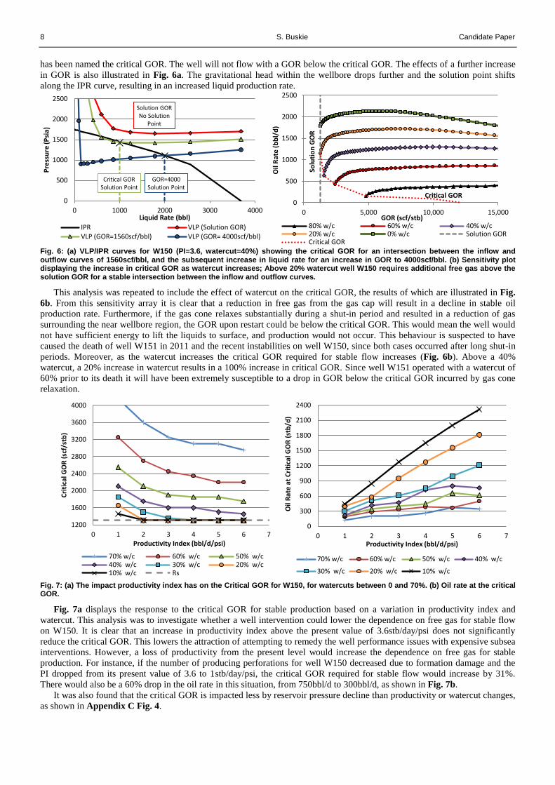
has been named the critical GOR. The well will not flow with a GOR below the critical GOR. The effects of a further increase
in GOR is also illustrated in Fig. 6a. The gravitational head within the wellbore drops further and the solution point shifts
along the IPR curve, resulting in an increased liquid production rate.
Fig. 6: (a) VLP/IPR curves for W150 (PI=3.6, watercut=40%) showing the critical GOR for an intersection between the inflow and outflow curves of 1560scf/bbl, and the subsequent increase in liquid rate for an increase in GOR to 4000scf/bbl. (b) Sensitivity plot displaying the increase in critical GOR as watercut increases; Above 20% watercut well W150 requires additional free gas above the solution GOR for a stable intersection between the inflow and outflow curves.
This analysis was repeated to include the effect of watercut on the critical GOR, the results of which are illustrated in Fig.
6b. From this sensitivity array it is clear that a reduction in free gas from the gas cap will result in a decline in stable oil
production rate. Furthermore, if the gas cone relaxes substantially during a shut-in period and resulted in a reduction of gas
surrounding the near wellbore region, the GOR upon restart could be below the critical GOR. This would mean the well would
not have sufficient energy to lift the liquids to surface, and production would not occur. This behaviour is suspected to have
caused the death of well W151 in 2011 and the recent instabilities on well W150, since both cases occurred after long shut-in
periods. Moreover, as the watercut increases the critical GOR required for stable flow increases (Fig. 6b). Above a 40%
watercut, a 20% increase in watercut results in a 100% increase in critical GOR. Since well W151 operated with a watercut of
60% prior to its death it will have been extremely susceptible to a drop in GOR below the critical GOR incurred by gas cone
relaxation.
Fig. 7: (a) The impact productivity index has on the Critical GOR for W150, for watercuts between 0 and 70%. (b) Oil rate at the critical GOR.
Fig. 7a displays the response to the critical GOR for stable production based on a variation in productivity index and
watercut. This analysis was to investigate whether a well intervention could lower the dependence on free gas for stable flow
on W150. It is clear that an increase in productivity index above the present value of 3.6stb/day/psi does not significantly
reduce the critical GOR. This lowers the attraction of attempting to remedy the well performance issues with expensive subsea
interventions. However, a loss of productivity from the present level would increase the dependence on free gas for stable
production. For instance, if the number of producing perforations for well W150 decreased due to formation damage and the
PI dropped from its present value of 3.6 to 1stb/day/psi, the critical GOR required for stable flow would increase by 31%.
There would also be a 60% drop in the oil rate in this situation, from 750bbl/d to 300bbl/d, as shown in Fig. 7b.
It was also found that the critical GOR is impacted less by reservoir pressure decline than productivity or watercut changes,
as shown in Appendix C Fig. 4.
Critical GOR Solution Point
GOR=4000 Solution Point
Solution GOR No Solution
Point
0
500
1000
1500
2000
2500
0 1000 2000 3000 4000
Pre
ssu
re (P
sia)
Liquid Rate (bbl)
IPR VLP (Solution GOR)VLP (GOR=1560scf/bbl) VLP (GOR= 4000scf/bbl)
Solu
tio
n G
OR
Critical GOR 0
500
1000
1500
2000
2500
0 5,000 10,000 15,000
Oil
Rat
e (
bb
l/d
)
GOR (scf/stb) 80% w/c 60% w/c 40% w/c20% w/c 0% w/c Solution GORCritical GOR
1200
1600
2000
2400
2800
3200
3600
4000
0 1 2 3 4 5 6 7
Cri
tica
l GO
R (
scf/
stb
)
Productivity Index (bbl/d/psi)
70% w/c 60% w/c 50% w/c40% w/c 30% w/c 20% w/c10% w/c Rs
0
300
600
900
1200
1500
1800
2100
2400
0 1 2 3 4 5 6 7
Oil
Rat
e a
t C
riti
cal G
OR
(st
b/d
)
Productivity Index (bbl/d/psi)
70% w/c 60% w/c 50% w/c 40% w/c
30% w/c 20% w/c 10% w/c
Candidate Paper Modelling the Impact of Gas Cone Relaxation on Well Performance 9
Mechanistic Modelling
A two-dimensional fine grid mechanistic reservoir model was created that represented the reservoir section around the heel
of well W150. This has 10’x100’x10’ grid blocks in the x-y-z direction. This is illustrated in Fig. 8, with a comparison
between the fine grid and coarse grid model. The coarse grid model represents the grid size utilised in the Mirren full field
model with an average grid size of 100’x100’x100’ in the x-y-z direction. The model has constant properties, with porosities
of 20%, 21.5% and 22% for the Forties, Lista and Maureen stratiographic layers respectively, a horizontal permeability of
15mD and kv/kh ratio of 0.01 within all layers. The other static rock and fluid properties match those provided in Table 2.
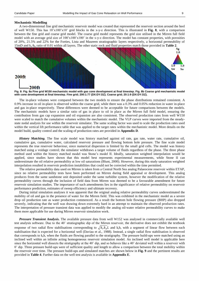
Fig. 8: Fig. 8a Fine grid W150 mechanistic model with gas cone development at final timestep. Fig. 8b Coarse grid mechanistic model with cone development at final timestep. Fine grid; 200:1:77 (DX:DY:DZ). Coarse grid; 20:1:9 (DX:DY:DZ).
The in-place volumes were compared between the two models to ensure the phase distributions remained consistent. A
0.9% increase in oil in-place is observed within the coarse grid, while there was a 0.3% and 0.05% reduction in water in-place
and gas in-place respectively. These differences were deemed to be acceptable for future comparisons between the models.
The mechanistic models have a similar ratio of gas in place to oil in place as the Mirren full field model, ensuring the
contribution from gas cap expansion and oil expansion are also consistent. The observed production rates from well W150
were scaled to match the cumulative volumes within the mechanistic model. The VLP curves were imported from the steady-
state nodal analysis for use within the reservoir simulator. The same scaling factor was used to scale the production rates used
within the vertical lift performance table that was applied to the target rates within the mechanistic model. More details on the
model build, quality control and the scaling of production rates are provided in Appendix D.
History Matching. The fine scale model was history matched against oil rate, gas rate, water rate, cumulative oil,
cumulative gas, cumulative water, calculated reservoir pressure and flowing bottom hole pressure. The fine scale model
represents the true reservoir behaviour, since numerical dispersion is limited by the small grid cells. The model was history
matched using a voidage control; the simulator withdraws a target volume of fluids regardless of the phase. The three phase
method used within the history matched model was Stone’s model II. Ideally, saturation weighted interpolation would be
applied, since studies have shown that this model best represents experimental measurements, while Stone II can
underestimate the oil relative permeability at low oil saturations (Blunt, 2000). However, during this study saturation weighted
interpolation resulted in reservoir prediction instabilities that could not be corrected within the time permitted.
The relative permeability data used on Mirren is taken from a Central North Sea analog Palaeocene reservoir within ETAP,
since no relative permeability tests have been performed on Mirren during field appraisal or development. This analog
produces from the same sandstone unit deposited under the same turbidite system, however the modification of the relative
permeability curves through the inclusion of field data from Mirren was deemed to be a favourable amendment for future
reservoir simulation studies. The importance of such amendments lies in the significance of relative permeability on reservoir
performance prediction, estimates of sweep efficiency and ultimate recovery.
During initial simulation analyses it was apparent that the original analog relative permeability curves underestimated the
mobility of oil and gas in the presence of water for the Mirren field. This was exhibited in the mechanistic model as a severe
drop oil production rate as water production commenced. As a result the bottom hole flowing pressure (BHP) also dropped
severely, indicating that the well was drawing down extremely hard in an attempt to maintain the observed production rates.
The interpretation of pressure transient data was applied to modify the analog oil-water relative permeability curves to make
them more applicable for use during Mirren reservoir simulation work.
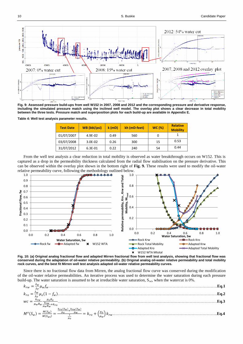
Pressure Transient Analysis. The available pressure data from well W152 was analysed in commercially available well
test analysis software. Due to the 40˚ stratiographic dip of the Mirren reservoir, the derivative does not exhibit the textbook
response of two radial flow stabilisations corresponding to √ and krh, with a segment of linear flow between each
stabilisation that is expected for a horizontal well (Daviau et al., 1988). Instead, a single radial flow stabilisation is observed
that corresponds to krh, when the fluids are flowing parallel to the stratigraphy. The pressure build-ups were matched using an
inclined well within an infinite acting homogeneous reservoir simulation model. An inclined well model is applicable here
since the horizontal well dissects the stratigraphy at the 40˚ dip, and so behaves like a 40˚ deviated well within a reservoir with
0˚ dip. Three pressure build-ups were of sufficient quality and length to allow a comparison between the total mobility within
the reservoir over time. The pressure build-ups and simulated matches are shown below in Fig. 9 and the pertinent results are
provided in Table 4. Further data on the well test analysis is available in Appendix E.
10 S. Buskie Candidate Paper
Fig. 9: Assessed pressure build-ups from well W152 in 2007, 2008 and 2012 and the corresponding pressure and derivative response, including the simulated pressure match using the inclined well model. The overlay plot shows a clear decrease in total mobility between the three tests. Pressure match and superposition plots for each build-up are available in Appendix E.
Table 4: Well test analysis parameter results.
Test Date WB (bbl/psi) k (mD) kh (mD-feet) WC (%) Relative Mobility
01/07/2007 4.9E-02 0.49 560 0 1
03/07/2008 3.0E-02 0.26 300 15 0.53
31/07/2012 6.3E-01 0.22 240 54 0.44
From the well test analysis a clear reduction in total mobility is observed as water breakthrough occurs on W152. This is
captured as a drop in the permeability thickness calculated from the radial flow stabilisation on the pressure derivative. This
can be observed within the overlay plot shown in the bottom right of Fig. 9. These results were used to modify the oil-water
relative permeability curve, following the methodology outlined below.
Fig. 10: (a) Original analog fractional flow and adapted Mirren fractional flow from well test analysis, showing that fractional flow was conserved during the adaptation of oil-water relative permeability. (b) Original analog oil-water relative permeability and total mobility rock curves, and the best fit Mirren well test analysis adapted oil-water relative permeability curves.
Since there is no fractional flow data from Mirren, the analog fractional flow curve was conserved during the modification
of the oil-water relative permeabilities. An iterative process was used to determine the water saturation during each pressure
build-up. The water saturation is assumed to be at irreducible water saturation, Swi, when the watercut is 0%.
…………………………………………………………………………………………………………….Eq.1
( )………………………………………………………………………………………………………Eq.2
………………………………………………………………………………………………………Eq.3
( ) ( )
( )
( )
( )
(
) …………………………………………………………………..Eq.4
0.0
0.1
0.2
0.3
0.4
0.5
0.6
0.7
0.8
0.9
1.0
0.0 0.2 0.4 0.6 0.8 1.0
Frac
tio
nal
Flo
w, f
w
Water Saturation, Sw Rock fw Adapted fw W152 WTA
0.0
0.2
0.4
0.6
0.8
1.0
0.0 0.2 0.4 0.6 0.8 1.0
Re
lati
ve p
erm
eab
ility
, Kro
, K
rw a
nd
To
tal
Mo
bili
ty, M
Tota
l
Water Saturation, Sw Rock Krw Rock Kro
Rock Total Mobility Adapted Krw
Adapted Kro Adapted Total Mobility
W152 WTA Mtotal

Candidate Paper Modelling the Impact of Gas Cone Relaxation on Well Performance 11
Eq.1 and Eq.2 provide the relative permeability in the presence of water and oil respectively. Fractional flow was altered,
until the watercut given by Eq.3 matched the observed watercut for each pressure build-up. Once the water saturation was
known during each well test, the total mobility could be plotted on the oil-water relative permeability graph, as shown in Fig.
11b. From here the relative permeability of oil, kro, and water, krw, were adjusted, while maintaining the fractional flow of the
system, to alter the normalised relative permeability (Eq.4) so that the end result best fit the three relative mobility data points
provided by the well test analysis.
For a water saturation of 0.46 the analog rock curves provide a normalised relative mobility of 13%. This water saturation
is equivalent to a watercut of 15%, as found using the fractional flow iterative method. From the analysis of the pressure build-
up at a 15% watercut (water saturation of 0.46) the normalised relative mobility is 53%. This indicates that the analog rock
curves severely underestimate the total mobility of the Mirren field. The normalised relative mobility is underestimated further
at higher water saturations; the analog rock curves dictate a normalised relative mobility of only 8% at a water saturation of
0.53, while the well test analysis from the 2012 pressure build-up (water saturation of 0.53) shows that the normalised relative
mobility is 44%.
Fig. 11: (a) Application of increased mobility from well test analysis during use in the mechanistic reservoir simulator. (b) Highlights the influence the increased mobility has on the simulated bottom hole pressure as water breaks through.
The impact of the modified relative permeability curves is illustrated in Fig. 11. Using the original analog curves, as water
production begins the bottom hole pressure drops dramatically. Ultimately the BHP reaches the pressure limit, set here to be
atmospheric pressure to demonstrate the severity of the required drawdown to match the oil and gas production rates. Even
with the impractical pressure drawdown the observed production rates cannot be achieved. The application of the increased
mobility relative permeability curves is successful in allowing the production of oil, gas and water to be matched against the
field observations, while also ensuring the simulated bottom hole pressure matches the observed bottom hole pressure.
Grid Comparison. A comparison between the cumulative volumes produced within the fine and coarse grid simulation
model presented some differences. The reason for this is due to the effects of numerical dispersion. The coarse grid model has
only three cells between the gas-oil contact and the well perforation, while the fine grid model has over ten times more. Gas
production is therefore increased within the coarse grid model when compared to the fine grid model, as shown in Table 5. As
the model was controlled by total produced volumes, an increase in produced gas resulted in a reduction in oil and water
production. To account for these effects the gas-oil relative permeability curves were upscaled.
Since numerical dispersion increases the gas production rate, the aim of the upscaling was to delay the breakthrough of gas
and reduce the cumulative gas production. The upscaling was implemented through the creation of pseudo relative
permeability gas-oil curves. These were adaptations of the analog gas-oil relative permeability curves which remained
unchanged during the well test analysis modifications of the oil-water curves. Since the critical gas saturation is the minimum
saturation required for the flow of gas from one pore to the next, or in simulation terms, from one grid block to the next, it was
adapted during the upscaling to delay gas production. The critical gas saturation was increased to inhibit the flow of gas. This
adaptation is also applicable since it increases the average saturation behind the flood front derived from the fractional flow.
This provides a more favourable gas displacement process, which would be expected from a steeply dipping reservoir that is
influenced by gravity (Dake, 1978). It was assumed that the oil relative permeability in the presence of gas, krog, would remain
at its effective relative permeability (krog=1) until the critical gas saturation is reached. The pseudo curves are detailed in Fig.
12. The impact that the pseudo gas-oil curves have on cumulative oil production are shown in Fig. 13. Ultimately, an increase
in critical gas saturation from 3% to 7% provides the best match between fine and coarse simulation grids for Mirren. The
percentage difference between the fine and coarse grid cumulative oil production is displayed in Fig. 13b. The impact these
pseudo curves makes on the production rates of oil, water and gas can be found in Appendix D Fig. 5-7.
0
0.1
0.2
0.3
0.4
0.5
0.6
0.7
0.8
0.9
1
0
500
1000
1500
2000
2500
3000
3500
4000
4500
5000
01/01/02 31/12/04 01/01/08 01/01/11 01/01/14
Wat
er
Cu
t, F
ract
ion
Bo
tto
m H
ole
Pre
ssu
re (
psi
a)
BHP Adapted Curve BHP Rock CurveBHP Observed w/c Adapted Curvew/c Rock Curves w/c Observed
0
0.1
0.2
0.3
0.4
0
400
800
1200
1600
2000
01/01/12 09/06/12 16/11/12 25/04/13
Wat
er
Cu
t, F
ract
ion
Bo
tto
m H
ole
Pre
ssu
re (
psi
a)
BHP Adapted Curve BHP Rock Curve
BHP Observed w/c Rock Curves
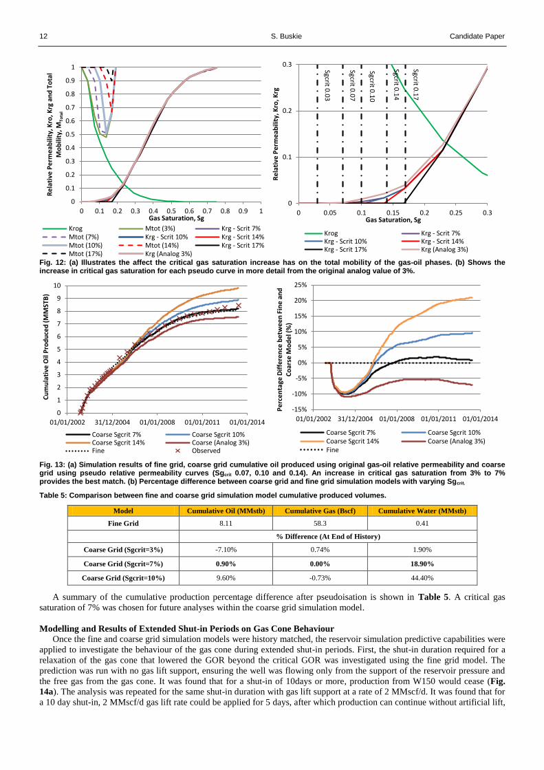
12 S. Buskie Candidate Paper
Fig. 12: (a) Illustrates the affect the critical gas saturation increase has on the total mobility of the gas-oil phases. (b) Shows the increase in critical gas saturation for each pseudo curve in more detail from the original analog value of 3%.
Fig. 13: (a) Simulation results of fine grid, coarse grid cumulative oil produced using original gas-oil relative permeability and coarse grid using pseudo relative permeability curves (Sgcrit 0.07, 0.10 and 0.14). An increase in critical gas saturation from 3% to 7% provides the best match. (b) Percentage difference between coarse grid and fine grid simulation models with varying Sgcrit.
Table 5: Comparison between fine and coarse grid simulation model cumulative produced volumes.
Model Cumulative Oil (MMstb) Cumulative Gas (Bscf) Cumulative Water (MMstb)
Fine Grid 8.11 58.3 0.41
% Difference (At End of History)
Coarse Grid (Sgcrit=3%) -7.10% 0.74% 1.90%
Coarse Grid (Sgcrit=7%) 0.90% 0.00% 18.90%
Coarse Grid (Sgcrit=10%) 9.60% -0.73% 44.40%
A summary of the cumulative production percentage difference after pseudoisation is shown in Table 5. A critical gas
saturation of 7% was chosen for future analyses within the coarse grid simulation model.
Modelling and Results of Extended Shut-in Periods on Gas Cone Behaviour
Once the fine and coarse grid simulation models were history matched, the reservoir simulation predictive capabilities were
applied to investigate the behaviour of the gas cone during extended shut-in periods. First, the shut-in duration required for a
relaxation of the gas cone that lowered the GOR beyond the critical GOR was investigated using the fine grid model. The
prediction was run with no gas lift support, ensuring the well was flowing only from the support of the reservoir pressure and
the free gas from the gas cone. It was found that for a shut-in of 10days or more, production from W150 would cease (Fig.
14a). The analysis was repeated for the same shut-in duration with gas lift support at a rate of 2 MMscf/d. It was found that for
a 10 day shut-in, 2 MMscf/d gas lift rate could be applied for 5 days, after which production can continue without artificial lift,
0
0.1
0.2
0.3
0.4
0.5
0.6
0.7
0.8
0.9
1
0 0.1 0.2 0.3 0.4 0.5 0.6 0.7 0.8 0.9 1
Re
lati
ve P
erm
eab
ility
, Kro
, Krg
an
d T
ota
l M
ob
ility
, MTo
tal
Gas Saturation, Sg
Krog Mtot (3%) Krg - Scrit 7%Mtot (7%) Krg - Scrit 10% Krg - Scrit 14%Mtot (10%) Mtot (14%) Krg - Scrit 17%Mtot (17%) Krg (Analog 3%)
Sgcrit 0.0
3
Sgcrit 0.0
7
Sgcrit 0.1
0
Sgcrit 0.1
4
Sgcrit 0.1
7
0
0.1
0.2
0.3
0 0.05 0.1 0.15 0.2 0.25 0.3
Re
lati
ve P
erm
eab
ility
, Kro
, Krg
Gas Saturation, Sg
Krog Krg - Scrit 7%Krg - Scrit 10% Krg - Scrit 14%Krg - Scrit 17% Krg (Analog 3%)
0
1
2
3
4
5
6
7
8
9
10
01/01/2002 31/12/2004 01/01/2008 01/01/2011 01/01/2014
Cu
mu
lati
ve O
il P
rod
uce
d (
MM
STB
)
Coarse Sgcrit 7% Coarse Sgcrit 10%Coarse Sgcrit 14% Coarse (Analog 3%)Fine Observed
-15%
-10%
-5%
0%
5%
10%
15%
20%
25%
01/01/2002 31/12/2004 01/01/2008 01/01/2011 01/01/2014
Pe
rce
nta
ge D
iffe
ren
ce b
etw
ee
n F
ine
an
d
Co
arse
Mo
de
l (%
)
Coarse Sgcrit 7% Coarse Sgcrit 10%Coarse Sgcrit 14% Coarse (Analog 3%)Fine
Candidate Paper Modelling the Impact of Gas Cone Relaxation on Well Performance 13
as shown in Fig. 14a. Indeed five days of gas lift at 2 MMscf/d can be applied to regain stable flow for shut-ins up to 60 days
in length within the fine grid simulation model. The results are different using the coarse grid model (Fig. 14b), despite the
pseudoisation of relative permeabilities. The difference is clear when the two recovery matrices are compared.
Fig. 14: (a) Fine grid shut-in and recovery matrix, including gas lift rate and duration. (b) Equivalent coarse grid matrix. It is clear that the coarse grid predicts more optimistic recovery times than the fine grid for the same gas lift usage and shut-in duration.
Although the upscaling provided a good comparison between the fine and coarse models on production rates and
cumulative volumes, the relaxation of the gas cone during an extended shut-in duration is not well represented.
The data from Fig. 14 can be compared against the field observed data from Fig. 4 by applying the same logarithmic trend
through the data. This highlights that both fine and coarse grid mechanistic models predict optimistic recovery times.
Fig. 15: (a) Simulation recovery times compared to an uncertainty range given to well W150 observed data (from Fig. 4), based on uncertainties from qualitative assessment of stable flow, and trend fitting bias towards the June 2012 shut-in. (b) Relative GOR at restart of well W150 within the fine, coarse (with pseudo-curves) and coarse without critical gas saturation modification.
The optimism is caused in part by 50% underestimate in oil rate over the final two years of field production within both the
fine and coarse grid simulation models. This is shown in Fig. 13a as a slight reduction in cumulative oil production when
compared to the observed production data points. Since the gas rates were matched by the simulator the net result is an
increased GOR. This means that there is a larger quantity of gas surrounding the well within the reservoir and the well is less
susceptible to the impact of gas cone relaxation. Appendix D Fig. 9 shows that this is not an issue for future analysis.
The ratio of the GOR upon restart within the mechanistic models compared to the pre-shut-in GOR has been plotted in Fig.
15b for various shut-in durations. This has been called the relative GOR. This illustrates the difficulty that the coarse grid
simulation model, with or without pseudoisation, has in capturing the movement of free gas during a shut-in. After a 1 day
shut-in the GOR within the fine grid model drops by 52%, resulting in a relative GOR of 0.48. Both coarse grid models (with
and without pseudoisation) predict that the relative GOR upon restart will be 0.97 for the same shut-in duration. As the shut-in
duration increases the pseudoisation does provide improved results over the original analog relative permeability curves.
As the recovery time increases the match between the relative GOR captured within the fine grid and the coarse grid with
the pseudo curves improves further. This is illustrated in the relative GOR contour maps of Fig. 16. It can be seen that after 25
days of recovery the relative GOR from the coarse grid model with the 7% Sgcrit matches the fine grid response (Fig. 16 left
and centre left). The recovery behaviour of the producing GOR is overestimated using the original analog rock curves (Fig.
16 centre right). It was found that the original rock curves applied in a coarse grid model present a 3% overestimate of
cumulative oil production after restart during a 100 day recovery period, after a 100 day shut-in. The pseudoisation generates a
0.2% error when compared to the fine grid over the same period. It is only the most severe GOR contrasts that are not captured
within these coarse grid models. Such low relative GORs are observed within the first ten days of recovery while the gas cone
redevelops. This means a coarse grid simulation model may predict continued production after a shut-in where in reality the
well will not flow, as the GOR has dropped below the critical GOR. The impact of this could be large, since production
profiles may be generated for a well based on the results from a coarse grid full-field model scale reservoir simulation model
that does not capture the full susceptibility to production losses that can be incurred through gas cone relaxation after a shut-in.
Gas Lift on for
(Days)0
Gas lift rate
(MMscf/d)0 1 2 3 3.5 1 2 3 3.5 1 2 3 3.5 1 2 3 3.5
10 n y y y y y y y y y y y y y y y y
20 n y y y y y y y y y y y y y y y y
30 n y y y y y y y y y y y y y y y y
40 n y y y y y y y y y y y y y y y y
50 n n y y y y y y y y y y y y y y y
60 n n y y y y y y y y y y y y y y y
70 n n n n n y y y y y y y y y y y y
80 n n n n n y y y y y y y y y y y y
90 n n n n n n n y y y y y y y y y y
100 n n n n n n n n n n y y y y y y y
110 n n n n n n n n n n y y y y y y y
120 n n n n n n n n n n n y y y y y y
130 n n n n n n n n n n n n n n y y y
140 n n n n n n n n n n n n n n y y y
150 n n n n n n n n n n n n n n n y y
160 n n n n n n n n n n n n n n n y y
Fine Grid Simulation Model
5 10 15 20
Shut-in
duration
(Days)
Gas Lift on for
(Days)0
Gas lift rate
(MMscf/d)0 1 2 3 3.5 1 2 3 3.5 1 2 3 3.5 1 2 3 3.5
10 y y y y y y y y y y y y y y y y y
20 y y y y y y y y y y y y y y y y y
30 y y y y y y y y y y y y y y y y y
40 y y y y y y y y y y y y y y y y y
50 y y y y y y y y y y y y y y y y y
60 y y y y y y y y y y y y y y y y y
70 y y y y y y y y y y y y y y y y y
80 n y y y y y y y y y y y y y y y y
90 n y y y y y y y y y y y y y y y y
100 n n n n n n y y y y y y y y y y y
110 n n n n n n n n n n y y y y y y y
120 n n n n n n n n n n y y y y y y y
130 n n n n n n n n n n n n n n y y y
140 n n n n n n n n n n n n n n n y y
150 n n n n n n n n n n n n n n n n n
160 n n n n n n n n n n n n n n n n n
Coarse Grid Simulation Model (With 7% Critical Gas Saturation)
20
Shut-in
duration
(Days)
5 10 15
0
10
20
30
40
50
0 10 20 30 40 50 60 70 80 90 100 110 120 130 140
Re
cove
ry T
ime
(D
ays)
Shut-in Duration (Days) Field Observed Range Coarse 2MMscf/d
Fine 2MMscf/d
0
0.2
0.4
0.6
0.8
1
1.2
0 20 40 60 80 100
Re
lati
ve G
OR
at
Re
star
t
Shut-in Duration (Days)
Pre-Shut-in GOR Fine
Coarse (Sgcrit 7%) Coarse (Original 3%)
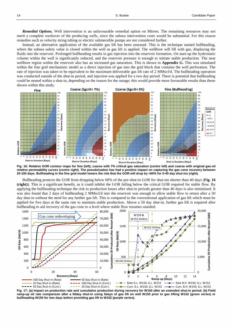
14 S. Buskie Candidate Paper
Remedial Options. Well intervention is an unfavourable remedial option on Mirren. The remaining resources may not
merit a complete workover of the producing wells, since the subsea intervention costs would be substantial. For this reason
remedies such as velocity string tubing or electric submersible pumps are not considered further.
Instead, an alternative application of the available gas lift has been assessed. This is the technique named bullheading,
where the subsea safety value is closed within the well as gas lift is applied. The wellbore will fill with gas, displacing the
fluids into the reservoir. Prolonged bullheading results in gas injection into the reservoir formation. On start-up the hydrostatic
column within the well is significantly reduced, and the reservoir pressure is enough to initiate stable production. The near
wellbore region within the reservoir also has an increased gas saturation. This is shown in Appendix G. This was simulated
within the fine grid mechanistic model as a direct injection of gas into the grid block that contains the well perforation. The
rate of injection was taken to be equivalent to the maximum deliverable gas lift rate of 2 MMscf/d. The bullheading operation
was conducted outside of the shut-in period, and injection was applied for a two day period. There is potential that bullheading
could be nested within a shut-in, depending on the reason for the outage; this would provide more favourable results than those
shown within this study.
Fig. 16: Relative GOR contour maps for fine (left), coarse with 7% critical gas saturation (centre left) and coarse with original gas-oil relative permeability curves (centre right). The pseudoisation has had a positive impact on capturing the gas cone recovery between 20-100 days. Bullheading in the fine grid model lowers the risk that the GOR will drop by >60% for 0-40 day shut-ins (right).
Bullheading protects the GOR from dropping below 60% of the pre-shut-in GOR for shut-ins shorter than 40 days (Fig. 16
(right)). This is a significant benefit, as it could inhibit the GOR falling below the critical GOR required for stable flow. By
applying the bullheading technique the risk to production losses after shut-in periods greater than 40 days is also minimised. It
was also found that 2 days of bullheading 2 MMscf/d into the reservoir was enough to allow stable flow to return after a 50
day shut-in without the need for any further gas lift. This is compared to the conventional application of gas lift which must be
applied for five days at the same rate to maintain stable production. Above a 50 day shut-in, further gas lift is required after
bullheading to aid recovery of the gas cone to a level where stable flow resumes unaided.
Fig. 17: (a) Impact on production rate and cumulative production during recovery for W150 after an extended shut-in period. (b) Field ramp-up oil rate comparison after a 50day shut-in using 5days of gas lift on well W150 prior to gas lifting W152 (green series) or bullheading W150 for two days before providing gas lift to W152 (purple series).
0
10,000
20,000
30,000
40,000
50,000
60,000
70,000
80,000
0
200
400
600
800
1000
1200
1400
1600
0 20 40 60
Cu
mu
lati
ve O
il P
rod
uce
d a
fte
r R
est
art
(bb
l)
Oil
Rat
e (
bb
l/d
)
Recovery (Days) 100 Day Shut-in (Rate) 50 Day Shut-in (Rate)10 Day Shut-in (Rate) 100 Day Shut-in (Cum.)50 Day Shut-in (Cum.) 10 Day Shut-in (Cum.)
Gas cone redeveloping W150 & W152 Online
W152 Online
W150 Online
0
5,000
10,000
15,000
20,000
0
500
1000
1500
2000
0 2 4 6 8 10 12 14
Cu
mu
lati
ve O
il P
rod
uct
ion
aft
er
Re
star
t (b
bl)
Oil
Rat
e (
bb
l/d
)
Ramp-up (Days)
Rate G.L. W150, G.L. W152 Rate B.H. W150, G.L. W152Cum. G.L. W150, G.L. W152 Cum. B.H. W150, G.L. W152
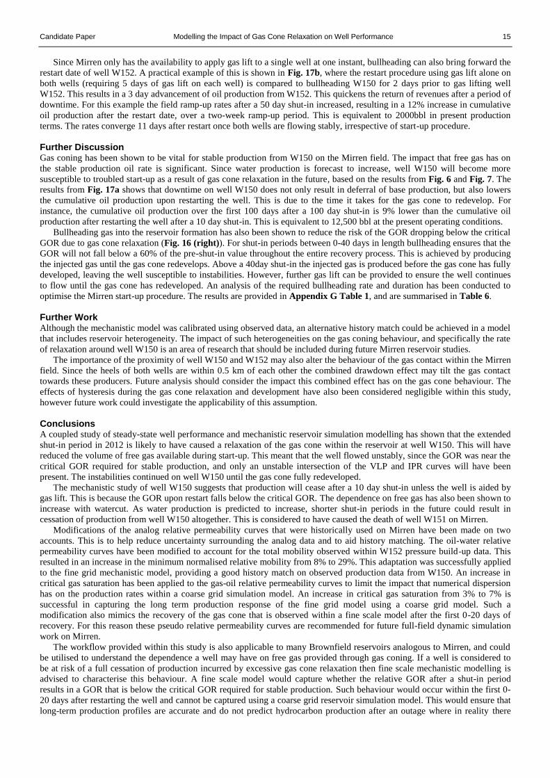
Candidate Paper Modelling the Impact of Gas Cone Relaxation on Well Performance 15
Since Mirren only has the availability to apply gas lift to a single well at one instant, bullheading can also bring forward the
restart date of well W152. A practical example of this is shown in Fig. 17b, where the restart procedure using gas lift alone on
both wells (requiring 5 days of gas lift on each well) is compared to bullheading W150 for 2 days prior to gas lifting well
W152. This results in a 3 day advancement of oil production from W152. This quickens the return of revenues after a period of
downtime. For this example the field ramp-up rates after a 50 day shut-in increased, resulting in a 12% increase in cumulative
oil production after the restart date, over a two-week ramp-up period. This is equivalent to 2000bbl in present production
terms. The rates converge 11 days after restart once both wells are flowing stably, irrespective of start-up procedure.
Further Discussion Gas coning has been shown to be vital for stable production from W150 on the Mirren field. The impact that free gas has on
the stable production oil rate is significant. Since water production is forecast to increase, well W150 will become more
susceptible to troubled start-up as a result of gas cone relaxation in the future, based on the results from Fig. 6 and Fig. 7. The
results from Fig. 17a shows that downtime on well W150 does not only result in deferral of base production, but also lowers
the cumulative oil production upon restarting the well. This is due to the time it takes for the gas cone to redevelop. For
instance, the cumulative oil production over the first 100 days after a 100 day shut-in is 9% lower than the cumulative oil
production after restarting the well after a 10 day shut-in. This is equivalent to 12,500 bbl at the present operating conditions.
Bullheading gas into the reservoir formation has also been shown to reduce the risk of the GOR dropping below the critical
GOR due to gas cone relaxation (Fig. 16 (right)). For shut-in periods between 0-40 days in length bullheading ensures that the
GOR will not fall below a 60% of the pre-shut-in value throughout the entire recovery process. This is achieved by producing
the injected gas until the gas cone redevelops. Above a 40day shut-in the injected gas is produced before the gas cone has fully
developed, leaving the well susceptible to instabilities. However, further gas lift can be provided to ensure the well continues
to flow until the gas cone has redeveloped. An analysis of the required bullheading rate and duration has been conducted to
optimise the Mirren start-up procedure. The results are provided in Appendix G Table 1, and are summarised in Table 6.
Further Work Although the mechanistic model was calibrated using observed data, an alternative history match could be achieved in a model
that includes reservoir heterogeneity. The impact of such heterogeneities on the gas coning behaviour, and specifically the rate
of relaxation around well W150 is an area of research that should be included during future Mirren reservoir studies.
The importance of the proximity of well W150 and W152 may also alter the behaviour of the gas contact within the Mirren
field. Since the heels of both wells are within 0.5 km of each other the combined drawdown effect may tilt the gas contact
towards these producers. Future analysis should consider the impact this combined effect has on the gas cone behaviour. The
effects of hysteresis during the gas cone relaxation and development have also been considered negligible within this study,
however future work could investigate the applicability of this assumption.
Conclusions A coupled study of steady-state well performance and mechanistic reservoir simulation modelling has shown that the extended
shut-in period in 2012 is likely to have caused a relaxation of the gas cone within the reservoir at well W150. This will have
reduced the volume of free gas available during start-up. This meant that the well flowed unstably, since the GOR was near the
critical GOR required for stable production, and only an unstable intersection of the VLP and IPR curves will have been
present. The instabilities continued on well W150 until the gas cone fully redeveloped.
The mechanistic study of well W150 suggests that production will cease after a 10 day shut-in unless the well is aided by
gas lift. This is because the GOR upon restart falls below the critical GOR. The dependence on free gas has also been shown to
increase with watercut. As water production is predicted to increase, shorter shut-in periods in the future could result in
cessation of production from well W150 altogether. This is considered to have caused the death of well W151 on Mirren.
Modifications of the analog relative permeability curves that were historically used on Mirren have been made on two
accounts. This is to help reduce uncertainty surrounding the analog data and to aid history matching. The oil-water relative
permeability curves have been modified to account for the total mobility observed within W152 pressure build-up data. This
resulted in an increase in the minimum normalised relative mobility from 8% to 29%. This adaptation was successfully applied
to the fine grid mechanistic model, providing a good history match on observed production data from W150. An increase in
critical gas saturation has been applied to the gas-oil relative permeability curves to limit the impact that numerical dispersion
has on the production rates within a coarse grid simulation model. An increase in critical gas saturation from 3% to 7% is
successful in capturing the long term production response of the fine grid model using a coarse grid model. Such a
modification also mimics the recovery of the gas cone that is observed within a fine scale model after the first 0-20 days of
recovery. For this reason these pseudo relative permeability curves are recommended for future full-field dynamic simulation
work on Mirren.
The workflow provided within this study is also applicable to many Brownfield reservoirs analogous to Mirren, and could
be utilised to understand the dependence a well may have on free gas provided through gas coning. If a well is considered to
be at risk of a full cessation of production incurred by excessive gas cone relaxation then fine scale mechanistic modelling is
advised to characterise this behaviour. A fine scale model would capture whether the relative GOR after a shut-in period
results in a GOR that is below the critical GOR required for stable production. Such behaviour would occur within the first 0-
20 days after restarting the well and cannot be captured using a coarse grid reservoir simulation model. This would ensure that
long-term production profiles are accurate and do not predict hydrocarbon production after an outage where in reality there
16 S. Buskie Candidate Paper
would be none. This study has therefore shown that many long term production profiles for brownfield reservoirs may require
amendments if future extended shut-in periods are planned, yet have not been modelled discretely using a fine scale simulation
model. In such cases, following the methodology used during this study would reduce uncertainty surrounding the ultimate
recoverable reserves from a field and ensure that they are feasible.
This study has also show the applicability of bullheading gas into the reservoir formation as a remedial option for restarting
wells that have incurred severe gas cone relaxation. Bullheading flushes the dense fluids out of the wellbore, easing the initial
restart, while also providing additional free gas that can be produced before the gas cone redevelops and contacts the well.
On Mirren bullheading not only reduces the risk that the GOR will drop below the critical GOR during the recovery, but
can also advance the restart date of well W152. This can result in 12% increase in cumulative oil production over a two week
field ramp-up period, in some cases. This has a positive impact on the revenue provided by the field and is a particularly
favourable outcome after a long duration with no hydrocarbon production. The recommended restart procedure for Mirren
following future shut-ins is provided in Table 6.
Table 6: Recommended Mirren start-up procedure (Summarised from Appendix G Table 1)
Shut-in (Days) Proposed Start-up Procedure Reasoning
0 - 10 Natural Lift No artificial lift required
10 - 20 Gas lift Gas lift sufficient for stable recovery.
20 - 50 Bullhead (no further gas lift required) W152 Restart advancement of 3 days. 6MMscf saving.
50 - 70 Bullhead (with additional gas lift) W152 Restart advancement of 3 days. 6MMscf saving.
70 - 100 Bullhead (with additional gas lift) Reduced risk of initial instabilities with 0-5days of recovery
Acknowledgements The author would like to thank David O’Gorman and the rest of the ETAP RMT and BMT at BP for their support. Thanks are
given to Professor Zimmerman of Imperial College London for his guidance at the start of this project.
Nomenclature BH Bullheading L Well length, ft
Bo,w Oil or water formation volume factor, RB/STB Mo(Sw) Normalised relative mobility
EH Entire History M(Sw) Mobility of oil
fw Fractional flow M(Swi) Mobility of oil at irreducible water saturation
G.L. Gas lift MTOT Total mobility
h Reservoir thickness, ft PI Productivity index, STB/day/psi
kh Permeability thickness, mDft S.G. Specific gravity
kr Radial flow permeability, mD Sgcrit Critical gas saturation
kro Relative permeability of oil Sw Water saturation
krg Relative permeability of gas Swi Irreducible water saturation
krw Relative permeability of water λw/λT Relative mobility from well test
kx Horizontal permeability, mD μo,w Oil or water viscosity, cp
References Addington, D., 1981, An approach to gas-coning correlations for a large grid cell reservoir simulator: Journal of Petroleum Technology, no.
JPT 8332-PA.
Blunt, M., 2000, An empirical model for three-phase relative permeability: Society of Petroleum Engineers, no. SPE 56474.
Dake, L., 1978, Fundamentals of Reservoir Engineering: Amsterdam, Elsevier Science Publishers Ltd.
Daviau, F., G. Mouronval, G. Bourdarot, and P. Curutchet, 1988, Pressure analysis for horizontal wells: Society of Petroleum Engineers, no.
SPE 14251.
Dousi, N., C. Veeken, and P. Currie, 2005, Modelling the gas well liquid loading process: Society of Petroleum Engineers, no. SPE 95282.
Green, A., A. Gringarten, and T. Whittle, 2012, Multi-phase Well Testing to Calibrate Relative Permeability Measurements for Reservoir
Simulation: Society of Petroleum Engineers, no. SPE 154851.
Jr, J. D., B. Darlow, R. Kendal, and M. Wheeler, 1979, Self-adaptive Galerkin methods for one-dimensional two-phase immiscible flow:
Society of Petroleum Engineers, no. SPE 7679.
Meyer, H. I., 1954, Mechanics of Two Immiscible Fluids in Porous Media: Journal of Applied Physics, v. 25, no. 11, p. 1400,
doi:10.1063/1.1721576.
Muskat, M., and R. Wyckoff, 1935, An approximate theory of water coning in oil production: AIME.
Perrine, R., 1956, Analysis of Pressure-Buildup Curves: Drilling and Production Practice.
SPE/AAPG/WPC/SPEE, 2007, Petroleum Resources Management System: Richardson, Texas.
Sobocinski, D., and A. Cornelius, 1965, A correlation for predicting water coning time: Society of Petroleum Engineers, no. SPE 894.
Turner, R., M. Hubbard, and A. Dukler, 1969, Analysis and prediction of minimum flow rate for the continuous removal of liquids from gas
wells, Paper SPE 2198: Journal of Petroleum Technology, no. SPE 2198.
Welge, H., and A. Weber, 1964, Use of two-dimensional methods for calculating well coning behavior: Society of Petroleum Engineers, no.
SPE 892.
Woods, E. G., and A. K. Khurana, 1977, Pseudofunctions for Water Coning in a Three-Dimensional Reservoir Simulator: Society of
Petroleum Engineers, no. SPE 5525, doi:10.2118/5525-PA.

17
Appendices
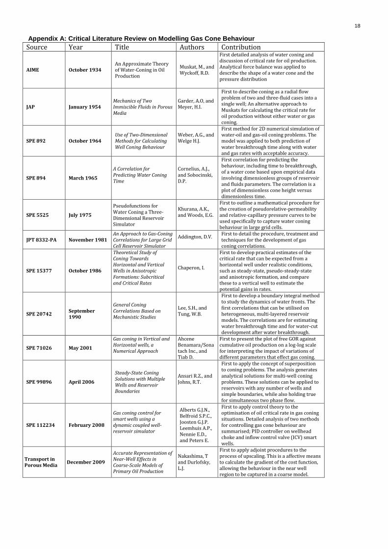
18
Appendix A: Critical Literature Review on Modelling Gas Cone Behaviour
Source Year Title Authors Contribution
AIME October 1934 An Approximate Theory of Water-Coning in Oil Production
Muskat, M., and Wyckoff, R.D.
First detailed analysis of water coning and discussion of critical rate for oil production. Analytical force balance was applied to describe the shape of a water cone and the pressure distribution
JAP January 1954 Mechanics of Two Immiscible Fluids in Porous Media
Garder, A.O, and Meyer, H.I.
First to describe coning as a radial flow problem of two and three-fluid cases into a single well; An alternative approach to Muskats for calculating the critical rate for oil production without either water or gas coning.
SPE 892 October 1964 Use of Two-Dimensional Methods for Calculating Well Coning Behaviour
Weber, A.G., and Welge H.J.
First method for 2D numerical simulation of water-oil and gas-oil coning problems. The model was applied to both prediction of water breakthrough time along with water and gas rates with acceptable accuracy.
SPE 894 March 1965
A Correlation for Predicting Water Coning Time
Cornelius, A.J., and Sobocinski, D.P.
First correlation for predicting the behaviour, including time to breakthrough, of a water cone based upon empirical data involving dimensionless groups of reservoir and fluids parameters. The correlation is a plot of dimensionless cone height versus dimensionless time.
SPE 5525 July 1975
Pseudofunctions for Water Coning a Three-Dimensional Reservoir Simulator
Khurana, A.K., and Woods, E.G.
First to outline a mathematical procedure for the creation of pseudorelative-permeability and relative-capillary pressure curves to be used specifically to capture water coning behaviour in large grid cells.
JPT 8332-PA November 1981 An Approach to Gas-Coning Correlations for Large Grid Cell Reservoir Simulator
Addington, D.V.
First to detail the procedure, treatment and techniques for the development of gas coning correlations.
SPE 15377 October 1986
Theoretical Study of Coning Towards Horizontal and Vertical Wells in Anisotropic Formations: Subcritical and Critical Rates
Chaperon, I.
First to develop practical estimates of the critical rate that can be expected from a horizontal well under realistic conditions, such as steady-state, pseudo-steady-state and anisotropic formation, and compare these to a vertical well to estimate the potential gains in rates.
SPE 20742 September 1990
General Coning Correlations Based on Mechanistic Studies
Lee, S.H., and Tung, W.B.
First to develop a boundary integral method to study the dynamics of water fronts. The first correlations that can be utilised on heterogeneous, multi-layered reservoir models. The correlations are for estimating water breakthrough time and for water-cut development after water breakthrough.
SPE 71026 May 2001
Gas coning in Vertical and Horizontal wells, a Numerical Approach
Ahcene Benamara/Sonatach Inc., and Tiab D.
First to present the plot of free GOR against cumulative oil production on a log-log scale for interpreting the impact of variations of different parameters that effect gas coning.
SPE 99896 April 2006
Steady-State Coning Solutions with Multiple Wells and Reservoir Boundaries
Ansari R.Z., and Johns, R.T.
First to apply the concept of superposition to coning problems. The analysis generates analytical solutions for multi-well coning problems. These solutions can be applied to reservoirs with any number of wells and simple boundaries, while also holding true for simultaneous two phase flow.
SPE 112234 February 2008
Gas coning control for smart wells using a dynamic coupled well-reservoir simulator
Alberts G.J.N., Belfroid S.P.C., Joosten G.J.P. Leemhuis A.P., Nennie E.D., and Peters E.
First to apply control theory to the optimisation of oil critical rate in gas coning situations. Detailed analysis of two methods for controlling gas cone behaviour are summarised; PID controller on wellhead choke and inflow control valve (ICV) smart wells.
Transport in Porous Media
December 2009
Accurate Representation of Near-Well Effects in Coarse-Scale Models of Primary Oil Production
Nakashima, T and Durlofsky, L.J.
First to apply adjoint procedures to the process of upscaling. This is a affective means to calculate the gradient of the cost function, allowing the behaviour in the near well region to be captured in a coarse model.

19
AIME (October 1934) [SPE 935144-G]
An Approximate Theory of Water-Coning in Oil Production
Authors:
Muskat, M., and Wyckoff, R.D.
Contribution to the understanding of gas cone relaxation in horizontal wells:
The first detailed analysis of water coning and discussion of critical rate for oil production.
Objective of Paper:
To present the physical principles that describe a water-oil interface during the production of oil from a vertical well that
partially penetrates the oil zone when the water remains in static equilibrium in the lower portion of the reservoir.
Methodology Used:
Analytical investigation of the oil flow system prior to water breakthrough. The water and oil are assumed to be in static
equilibrium, where a force balance between the pressure difference that increases the cone height and the pressure gradient due
to the acceleration of gravity is created. An iterative method is applied to describe the cone surface by assuming the pressure
function value p(r,z) since an explicit function for this would become too complex. The pressure distribution is taken from the
analysis of oil flow in a thin sand bed between two impermeable boundaries and into a well partially penetrating the sand.
Conclusions Reached:
1. The stability of a water cone is compromised when it has reached between 50 to 75% of the height to the bottom of the
well. The cones critical nature is displayed by the accelerated rise of the cone as the oil production rate is increased.
2. When breakthrough is near, the region of stability of the cone is sensitive to variations in oil rate which case small
changes in pressure differential.
3. The only means of eliminating bottom water when producing from a thin oil film is by reducing the oil rate below
economic values.
4. For a given average pressure differential, or production rate, a well that is flowing steadily will have a reduced cone
height compared with one which flows intermittently.
5. The analysis is the exact analogue of gas-coning. The physical description is identical when the system is inverted.
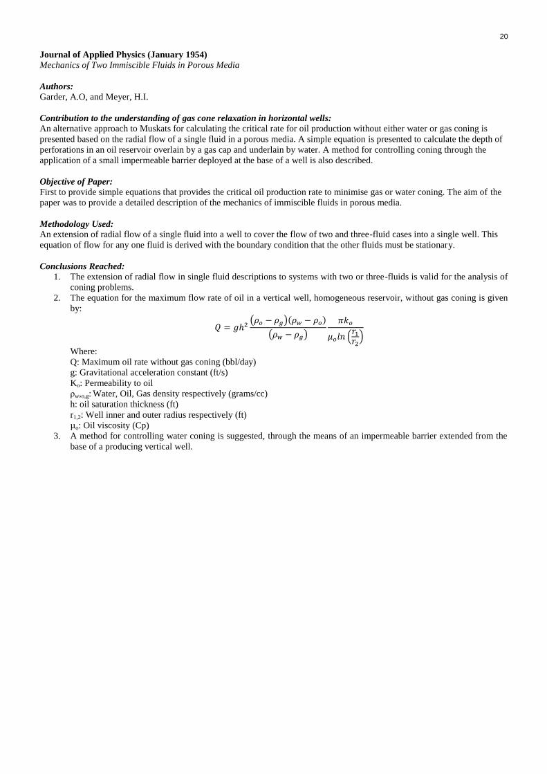
20
Journal of Applied Physics (January 1954)
Mechanics of Two Immiscible Fluids in Porous Media
Authors:
Garder, A.O, and Meyer, H.I.
Contribution to the understanding of gas cone relaxation in horizontal wells:
An alternative approach to Muskats for calculating the critical rate for oil production without either water or gas coning is
presented based on the radial flow of a single fluid in a porous media. A simple equation is presented to calculate the depth of
perforations in an oil reservoir overlain by a gas cap and underlain by water. A method for controlling coning through the
application of a small impermeable barrier deployed at the base of a well is also described.
Objective of Paper:
First to provide simple equations that provides the critical oil production rate to minimise gas or water coning. The aim of the
paper was to provide a detailed description of the mechanics of immiscible fluids in porous media.
Methodology Used:
An extension of radial flow of a single fluid into a well to cover the flow of two and three-fluid cases into a single well. This
equation of flow for any one fluid is derived with the boundary condition that the other fluids must be stationary.
Conclusions Reached:
1. The extension of radial flow in single fluid descriptions to systems with two or three-fluids is valid for the analysis of
coning problems.
2. The equation for the maximum flow rate of oil in a vertical well, homogeneous reservoir, without gas coning is given
by:
( )( )
( )
( )
Where:
Q: Maximum oil rate without gas coning (bbl/day)
g: Gravitational acceleration constant (ft/s)
Ko: Permeability to oil
ρw,o,g: Water, Oil, Gas density respectively (grams/cc)
h: oil saturation thickness (ft)
r1,2: Well inner and outer radius respectively (ft)
µo: Oil viscosity (Cp)
3. A method for controlling water coning is suggested, through the means of an impermeable barrier extended from the
base of a producing vertical well.

21
SPE 892 (October 1964)
Use of Two-Dimensional Methods for Calculating Well Coning Behaviour
Authors:
Weber, A.G., and Welge H.J.
Contribution to the understanding of gas cone relaxation in horizontal wells:
Outlines the first method for 2D numerical simulation of water-oil and gas-oil coning problems. Difficulties encountered
during simulations are described and overcome. The applicability of numerical simulations are proven by comparing the
results against both experimental data and field results. The model was applied to both prediction of water breakthrough with
acceptable accuracy and
Objective of Paper:
The paper was the first attempt of numerical simulation to apply two-phase, 2D calculations that use alternating direction
implicit procedure, to solve well coning calculations, such as limiting the maximum allowable saturation variation during a
simulation time step.
Methodology Used:
The alternating direction implicit procedure (ADIP) was used for the relaxation calculations of two-phase potentials using a
2D grid. A means of controlling unrealistic oscillations in phase saturations that were observed initially in fine grid blocks was
developed. This was done by constraining the allowable change in saturation for each time step. The requirement for small
grid blocks in the near wellbore region was also highlighted in the methodology.
Cone growth was tracked using the potentials and capillary pressure relationship to calculate saturation and pressure
distributions. The 2D method was validated by matching coning behaviour and produced water-oil ratio history of a laboratory
model and several producing wells.
Conclusions Reached:
1. The ADIP numerical method was adapted to solve problems of water and gas coning.
2. Once breakthrough occurs, special computational techniques must be used to ensure the accuracy of the results and to
limit computational costs.
3. Calculations matched the production history of actual producing wells experiencing water or free gas production and a
laboratory sandpacked model.
4. Experience gained from field studies shows the average vertical and horizontal permeability and the kv/kh ratio are
critical parameters for the accuracy of the calculations.

22
SPE 894 (March 1965)
A Correlation for Predicting Water Coning Time
Authors:
Cornelius, A.J., and Sobocinski, D.P.
Contribution to the understanding of gas cone relaxation in horizontal wells:
The first correlation for predicting the behaviour, including time to breakthrough, of a water cone based upon empirical data
involving dimensionless groups of reservoir and fluids parameters. Since the correlation groups are dimensionless they can be
applied out with water coning cases specifically covered by the experiments. The correlation is a plot of dimensionless cone
height versus dimensionless time.
Objective of Paper:
To further the analysis of the critical oil rate without water breakthrough to determine the time it takes for a cone to build up to
its incipient breakthrough position. The paper also aimed to improve the likelihood of solving coning problems using hand-
calculations. These hand-calculations, although not definitively accurate, allow the relative performance of wells to be
estimated. The dimensionless cone height versus dimensionless time correlation will permit estimates of the growth of some
water cones as they build from the static water-oil contact.
Methodology Used:
Empirical data combined with results from a computer program for a 2D incompressible system, and based partially on
dimensional analysis was used to develop the correlation. The basic coning equations for a water-oil system are solved using
finite difference calculus to resolve the partial differential equations into a set of algebraic equations. The experimental data
was observed on a single sand-packed laboratory model with a water-oil system.
Conclusions Reached:
1. The correlation of coning data allows estimates of water coning time for wells that are completed from the top of the
oil zone and are producing with a constant production rate.
2. The 2D numerical model matched results that were observed on the sand packed model. As such, the program was
considered reliable for studying factors that were not conveniently studied on the packed model.
3. Further work is required to ensure the applicability of the correlation in more general cases of water coning.

23
SPE 5525 (July 1975)
Pseudofunctions for Water Coning a Three-Dimensional Reservoir Simulator
Authors:
Khurana, A.K., and Woods, E.G.
Contribution to the understanding of gas cone relaxation in horizontal wells:
A detailed description of the mathematical procedure required to incorporate the results of a single-well, 2D, cylindrical or 3D
coning model into a coarse-grid 3D reservoir model.
Objective of Paper:
First to outline a mathematical procedure for the creation of pseudorelative-permeability and relative-capillary pressure curves
to be used specifically to capture water coning behaviour in large grid cells. First to outline a mathematical procedure for
incorporating the results of single well models fine-scale models into a 3D full field model grid scale reservoir model. The
procedure for developing pseudorelative-permeability and capillary-pressure curves is described, and the application of such
functions is shown in a large reservoir simulator model.
Methodology Used:
Partial integration of the equations of flow. The production performance from a detailed single well model is converted into a
set of time independent pseudorelative-permeability and capillary-pressure curves. The viscous forces and geometry of the
flow are dominant features for the creation of the pseudofunctions; hence, vertical equilibrium does not apply.
Conclusions Reached:
1. Coning functions can be applied to accurately capture the water breakthrough time, watercut and displacement
efficiency of a reservoir model dominated by bottom water drive.
2. When viscous forces are dominant over gravity forces, coning pseudos are independent of rate.
3. Pseudos describing well coning can be developed directly by integrating the performance of a detailed well model.

24
JPT 8332-PA (November 1981)
An Approach to Gas-Coning Correlations for Large Grid Cell Reservoir Simulator
Authors:
Addington, D.V.
Contribution to the understanding of gas cone relaxation in horizontal wells:
Procedure, treatment and techniques for the development of gas coning correlations are discussed throughout the paper. A
means of calculating an effective value of horizontal permeability and kv/kh, which are both used for the gas coning
correlations are described for a well with a heterogeneous description. A weighted averaging of horizontal and vertical
permeabilities in the oil zone from the perforations to the gas/oil contact with the weighting factor set as the layer thickness
divided by the average distance from the layer to the perforations. The horizontal permeabilities are averaged arithmetically
and the vertical permeabilities are averaged harmonically.
Objective of Paper:
Generalised gas coning correlations are developed specifically for a three-dimensional five layer Prudhoe Bay model. The
approach used for these gas coning correlations had the aim of developing general gas coning correlations that use individual
well parameters so that wells could be modelled individually without being grouped into well types.
Methodology Used:
Individual wells were modelled on two-dimensional fully implicit radial simulator. The behaviour of the gas coning was
correlated to the average oil column height above the perforated interval of the well. This can be calculated by the same
methodology for coarse and fine grid field models. It was assumed that the well receives little or no aquifer support. This was
based on field data for Prudhoe Bay oil wells.
The log of GLR was plotted against the average oil column height above the perforations. For a constant rate a linear trend is
observed in GLR with the oil column height after gas breakthrough occurred. The linear relationship is the basis for the
generalised correlations that were developed. Assumed that the residual oil saturation to gas flood was constant, at 0.25, which
introduces a <5% error in oil column height.
Conclusions Reached:
1. Generalised gas coning correlations created to predict the critical coning rate or to predict the GLR of a well after
coning has been achieved.
2. When the appropriate averaging of permeabilities has been applied it has been shown that these correlations can model
coning of wells with heterogeneous descriptions.

25
SPE 15377 (October 1986)
Theoretical Study of Coning Towards Horizontal and Vertical Wells in Anisotropic Formations: Subcritical and Critical Rates
Authors:
Chaperon, I.
Contribution to the understanding of gas cone relaxation in horizontal wells:
First to develop practical estimates of the critical rate that can be expected from a horizontal well under realistic conditions,
such as steady-state, pseudo-steady-state and anisotropic formation, and compare these to a vertical well to estimate the
potential gains in rates.
Objective of Paper:
To compare the behavioural differences between horizontal wells and vertical wells in anisotropic formations with respect to
gas coning.
Methodology Used:
Following the process outlined first by Muskat the equilibrium conditions are stated. Following this the description of viscous
flow potential relevant to the geometry of the flow created by a horizontal well under steady-state conditions is made. This is
later extended for pseudo-steady-state conditions for anisotropic formations.
Conclusions Reached:
1. A critical cone comes closer to a horizontal well than a vertical well.
2. Horizontal wells generally allow higher critical rates than vertical wells; however this advantage decreases with
increased anisotropy.

26
SPE 20742 (September 1990)
General Coning Correlations Based on Mechanistic Studies
Authors:
Lee, S.H., and Tung, W.B.
Contribution to the understanding of gas cone relaxation in horizontal wells:
First to develop a boundary integral method to study the dynamics of water fronts. The first correlations that can be utilised on
heterogeneous, multi-layered reservoir models. Creation of correlations that can be applied within reservoir simulators to
model sub-scale flow behaviour. The correlations are for estimating water breakthrough time and for water-cut development
after water breakthrough. Improved correlations were developed that include the effects of production rate, vertical and
horizontal permeabilities, fluid properties, relative permeabilities, aquifer thickness, completion location and interval size and
drainage radius on coning dynamics.
Objective of Paper:
To improve the correlations that describes coning behaviour for use in reservoir simulators or stand-alone programs. The
correlations are aimed at being applied during finite difference simulation to model sub-scale flow behaviour near a well.
Earlier correlations applied crude assumptions that limit their applicability to a wide range of problems, such as the steady
state approximation which cannot hold for cone development in general operating conditions.
Methodology Used:
Application of a boundary integral method for calculating saturation fronts. Mechanistic studies were conducted that
determined the key production, reservoir and well completion parameters on a simple case. These results were used to generate
improved coning correlations that could be extended to describe more general and complex systems.
Conclusions Reached:
1. Two sets of correlations were created allowing estimates of
2. Water breakthrough time
3. Water-cut development after water breakthrough
4. The correlations can be applied in stand-alone programs or reservoir simulations. They allow modelling of sub-grid
flow behaviour within the near wellbore region.

27
SPE 71026 (May 2001)
Gas coning in Vertical and Horizontal wells, a Numerical Approach
Authors:
Ahcene Benamara/Sonatach Inc., and Tiab D.
Contribution to the understanding of gas cone relaxation in horizontal wells:
A sensitivity study is performed to analyse the parameters that impact gas coning most significantly. A method for interpreting
the variation of different parameters that effect gas coning is suggested.
Plotting free GOR, GOR-Rs (the total GOR minus the ratio of the volume of gas dissolved within the well to the volume of oil)
against cumulative production (or recovery) on a log-log scale. A linear relationship between the two parameters is revealed
once breakthrough occurs.
Empirical correlations (from Well A, Hassi-R’mel field, Algeria) are developed to predict the critical oil rate, gas
breakthrough time and gas oil ratio (GOR) after breakthrough for both vertical and horizontal wells. The study showed that in
both horizontal and vertical wells the increase in the oil-gas density difference (increase in oil density and/or decrease in gas
density) delays the coning, decrease the GOR after breakthrough for the same cumulative oil production and increase ultimate
recovery. The results of the sensitivity study effecting gas coning are summarised.
Objective of Paper:
To determine the optimum oil flow rate of the well, and how to perforate a well subjected to coning. The paper summarises the
effects of variations in reservoir parameters on gas coning. Correlations for the breakthrough time, critical oil rate and gas oil
ratio after breakthrough were provided for both vertical and horizontal wells.
Methodology Used:
A numerical approach is applied to analyse gas coning in a 3D radial model, and gas dipping in a 3D irregular Cartesian
model. The paper assumed the GOC moves downward horizontally. Material balance is used to calculate the average column
height above perforations. Frontal advance theory is also applied for the expansion of gas cap and the downward movement of
the GOC (immiscible displacement) and therefore the fractional flow equation is employed.
Conclusions Reached:
1. Fine grid simulation models are required to accurately model coning problems
2. The use of horizontal wells to mitigate coning, when compared against vertical wells, was proven. The additional cost
of drilling and completing horizontal wells was not assessed during the project.

28
SPE 99896 (April 2006)
Steady-State Coning Solutions with Multiple Wells and Reservoir Boundaries
Authors:
Ansari R.Z., and Johns, R.T.
Contribution to the understanding of gas cone relaxation in horizontal wells:
The proposed analytical solutions provide coning solutions for multi-well problems using the concept of superposition. The
application of superposition allows simple and quick solutions when compared with simulation that can be applied to
reservoirs with any number of wells and simple boundaries, while also holding true for simultaneous two phase flow.
Objective of Paper:
To improve realism of previously existing analytical solutions. The current single-well analytical solutions were extended to
account for the behaviour from multiple wells and no-flow and constant pressure boundary conditions.
Methodology Used:
The principal of superposition is applied to superimpose existing single well coning solutions for single or two phase flow.
The relative permeability and capillary pressure effects of coning are also included. The analytical model assumes vertical
equilibrium and steady-state flow.
Conclusions Reached:
1. Superposition of single-well coning solutions is possible for single phase or two phase flow. The application of
superposition can be used to model multiple wells or simple reservoir boundaries that occur with standard well
patterns.
2. The results from the analytical solutions agree well with fine scale simulation studies for aspect ratios greater than 10.
For aspect ratios lower than 10 the critical oil rates are conservative from the vertical equilibrium solution.
3. Analytical solutions hold when steady-state is not achieved.
4. There is a possibility that coning may be modelled even in reservoirs where the hydrocarbon column thins over time.

29
SPE 112234 (February 2008)
Gas coning control for smart wells using a dynamic coupled well-reservoir simulator
Authors:
Alberts G.J.N., Belfroid S.P.C., Joosten G.J.P. Leemhuis A.P., Nennie E.D., and Peters E.
Contribution to the understanding of gas cone relaxation in horizontal wells:
Detailed analysis of two methods for controlling gas cone behaviour are summarised; PID controller on wellhead choke and
inflow control valve (ICV) smart wells. The redistribution due to gravity forces of the gas-oil-contact in the absence of
drawdown, i.e., gas cone relaxation, is noted.
Objective of Paper:
To demonstrate how the control of inflow from a gas cone as a natural lift can be used to increase the oil production rate from
a well. Two methods for controlling gas coning rate to maximise oil production are analysed and their effectiveness are
compared. These are the use of well head control and a PID controller on an ICV.
Methodology Used:
Steady state and dynamic well models were applied to a test case horizontal well that was coupled with dynamic reservoir
simulation to assess the benefits of controlling the gas fraction for maximum oil production. Control theory was applied; using
a PID controller two control set points were analysed to control the inflow when gas breakthrough occurs. The inflow was
compared on both wellhead choke control and controlled inflow from ICV’s.
Conclusions Reached:
1. PID control theory can be applied successfully to prevent full gas breakthrough while also being used to increase the
produced oil rate by tuning ICV settings to achieve an optimal well gas fraction.
2. Dynamic well model tied to dynamic reservoir model is advised. Coupled simulations could be significantly more
accurate in comparison to stand alone well or reservoir simulations.
3. Steady state model requires many lift curves to capture the ‘natural lift effect’
4. ICV’s control on gas rate provide optimum oil rate when compared to wellhead control.
30
Transport in Porous Media (December 2009)
Accurate Representation of Near-Well Effects in Coarse-Scale Models of Primary Oil Production
Authors:
Nakashima, T., and Durlofsky, L.J.
Contribution to the understanding of gas cone relaxation in horizontal wells:
First to apply adjoint procedures to the process of upscaling. The adjoint-based optimisation approach is an effective means to
calculate the gradient of the cost function, allowing behaviour in the near-well region to be captured in coarse-scale grid
blocks. Good correlation between fine-scale and coarse-scale simulations are shown throughout the paper, with both two-phase
and three-phase fluids.
Objective of Paper:
To apply the adjoint technique to the upscaling of properties from fine-scale to coarse-scale within near-well region models.
Three techniques are developed:
Near-well single-phase upscaling (NW1P)
Near-well multi-phase upscaling (NWMP)
Adaptive local-global multiphase upscaling (ALGMP)
Methodology Used:
Adjoint methods and gradient-based optimisation procedures were developed to give well-block parameters for multiphase
flow problems. These were created for two-phase and three-phase systems, where well-block functions are upscaled over a
local region surrounding the well.
Conclusions Reached:
1. Upscaled functions are determined for formation volume factors, solution gas-oil ratio, mobility functions and
transmissibilities.
2. Boundary conditions required for the local well model significantly impact the values of the upscaled parameters. A
simulation run performed on a global coarse-scale model is required to provide initial estimates of well-block
parameters.
3. The applicability of this technique was proven for heterogeneous reservoirs, black oil systems and a heavy oil system.
4. Near-well multiphase upscaling (NWMP) performs better than near-well single-phase upscaling (NW1P) in all case
examples.
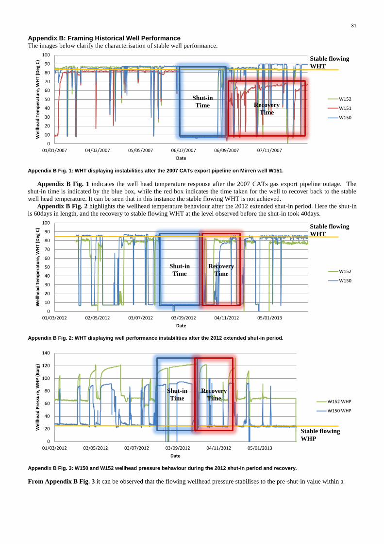
31
Appendix B: Framing Historical Well Performance The images below clarify the characterisation of stable well performance.
Appendix B Fig. 1: WHT displaying instabilities after the 2007 CATs export pipeline on Mirren well W151.
Appendix B Fig. 1 indicates the well head temperature response after the 2007 CATs gas export pipeline outage. The
shut-in time is indicated by the blue box, while the red box indicates the time taken for the well to recover back to the stable
well head temperature. It can be seen that in this instance the stable flowing WHT is not achieved.
Appendix B Fig. 2 highlights the wellhead temperature behaviour after the 2012 extended shut-in period. Here the shut-in
is 60days in length, and the recovery to stable flowing WHT at the level observed before the shut-in took 40days.
Appendix B Fig. 2: WHT displaying well performance instabilities after the 2012 extended shut-in period.
Appendix B Fig. 3: W150 and W152 wellhead pressure behaviour during the 2012 shut-in period and recovery.
From Appendix B Fig. 3 it can be observed that the flowing wellhead pressure stabilises to the pre-shut-in value within a
0
10
20
30
40
50
60
70
80
90
100
01/01/2007 04/03/2007 05/05/2007 06/07/2007 06/09/2007 07/11/2007
We
llhe
ad T
em
pe
ratu
re, W
HT
(De
g C
)
Date
W152
W151
W150
0
10
20
30
40
50
60
70
80
90
100
01/03/2012 02/05/2012 03/07/2012 03/09/2012 04/11/2012 05/01/2013
We
llhe
ad T
em
pe
ratu
re, W
HT
(De
g C
)
Date
W152
W150
0
20
40
60
80
100
120
140
01/03/2012 02/05/2012 03/07/2012 03/09/2012 04/11/2012 05/01/2013
We
llhe
ad P
ress
ure
, WH
P (
Bar
g)
Date
W152 WHP
W150 WHP
Stable flowing
WHT
Shut-in
Time Recovery
Time
Shut-in
Time
Recovery
Time
Stable flowing
WHT
Stable flowing
WHP
Shut-in
Time
Recovery
Time

32
shorter time period than the flowing WHT. This is because WHP is less sensitive to flowrate that the flowing WHT. This
qualitative assessment of shut-in duration and recovery time was repeated for all extended shut-in periods within each of the
three Mirren wells, throughout the entire field history. This is the data that was presented in Fig. 3 and Fig. 4.
Metastable Flow Analysis
The results of the metastable flow analysis that was conducted on the available data from well W151 and W152 throughout the
entire field history is provided below.
Appendix B Fig. 4: W150 daily average WHT.
Along with capturing whether metastable flow is present, these plots also help determine the operating efficiency (OE) of a
well. For instance, Appendix B Fig. 4 captures the OE for W150 throughout the years. Years with poor operating efficiency
have more days at the ambient WHT since the well is offline. 2012-2013 has seen the poorest OE at 60%. This is due to the
extended shut-in period, during the summer of 2012 that lasted 30days, and the resulting poor performance that was incurred
once well W150 was brought back online. The second worst year in terms of operational efficiency was between June 2007
and June 2008 which includes most of the time when production was ceased due to an outage on the CAT’s gas export
pipeline. This extended shut-in period initiated the well performance issues on W151 prior to its inability to flow in 2011.
Appendix B Fig. 5: W152 daily average WHT
As with W150, Appendix B Fig. 5 shows no characteristic signs of metastable flow within W152. A clear decline in
operating efficiency (OE) can also be seen on W152, with the periods between 2011 and 2013 displaying the most number of
0.00
10.00
20.00
30.00
40.00
50.00
60.00
70.00
80.00
90.00
100.00
0 50 100 150 200 250 300 350
Wllh
ead
Te
mp
era
ture
, W
HT
(De
g C
)
Time, Days 06/06/03-06/06/04 06/06/04-06/06/05 06/06/05-06/06/06 06/06/06-06/06/0706/06/07-06/06/08 06/06/08-06/06/09 06/06/09-06/06/10 06/06/10-06/06/1106/06/11-06/06/12 06/06/12-06/06/13
0
10
20
30
40
50
60
70
80
90
100
0 50 100 150 200 250 300 350
We
llhe
ad T
em
pe
ratu
re, W
HT
(De
g C
)
Time, Days 02/08/06-06/06/07 06/06/07-06/06/08 06/06/08-06/06/09 06/06/09-06/06/10
06/06/10-06/06/11 06/06/11-06/06/12 06/06/12-06/06/13
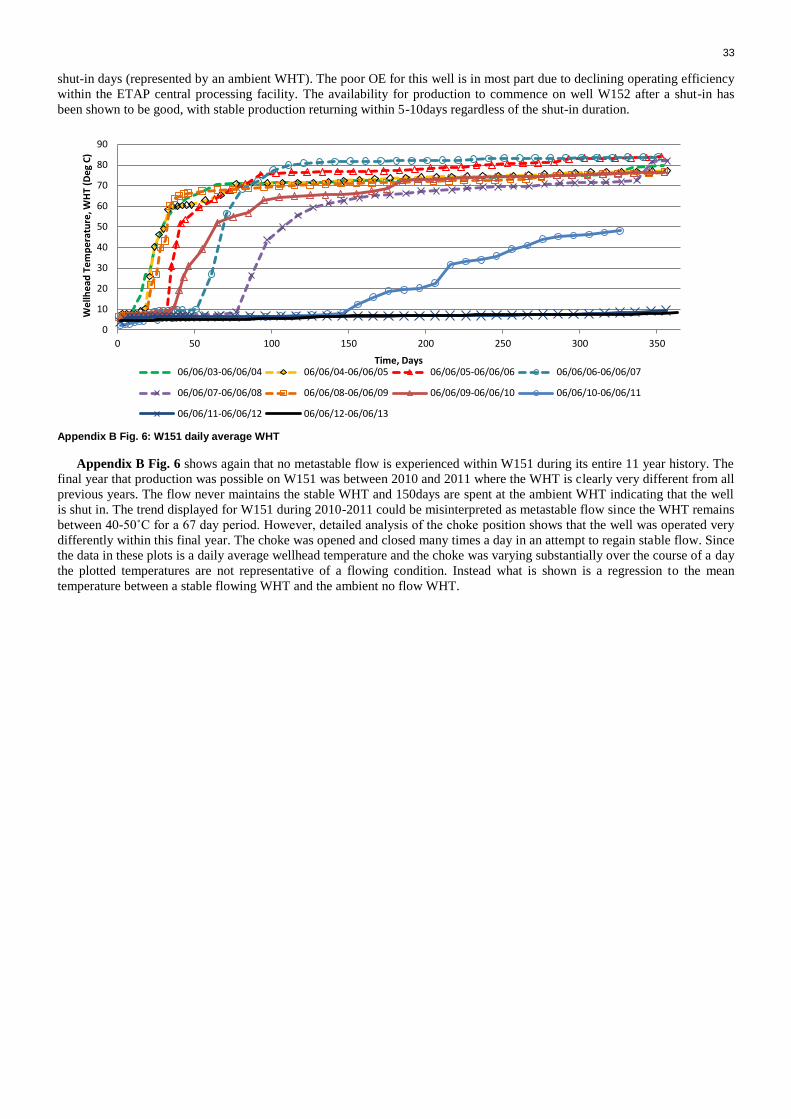
33
shut-in days (represented by an ambient WHT). The poor OE for this well is in most part due to declining operating efficiency
within the ETAP central processing facility. The availability for production to commence on well W152 after a shut-in has
been shown to be good, with stable production returning within 5-10days regardless of the shut-in duration.
Appendix B Fig. 6: W151 daily average WHT
Appendix B Fig. 6 shows again that no metastable flow is experienced within W151 during its entire 11 year history. The
final year that production was possible on W151 was between 2010 and 2011 where the WHT is clearly very different from all
previous years. The flow never maintains the stable WHT and 150days are spent at the ambient WHT indicating that the well
is shut in. The trend displayed for W151 during 2010-2011 could be misinterpreted as metastable flow since the WHT remains
between 40-50˚C for a 67 day period. However, detailed analysis of the choke position shows that the well was operated very
differently within this final year. The choke was opened and closed many times a day in an attempt to regain stable flow. Since
the data in these plots is a daily average wellhead temperature and the choke was varying substantially over the course of a day
the plotted temperatures are not representative of a flowing condition. Instead what is shown is a regression to the mean
temperature between a stable flowing WHT and the ambient no flow WHT.
0
10
20
30
40
50
60
70
80
90
0 50 100 150 200 250 300 350
We
llhe
ad T
em
pe
ratu
re, W
HT
(De
g C
)
Time, Days 06/06/03-06/06/04 06/06/04-06/06/05 06/06/05-06/06/06 06/06/06-06/06/07
06/06/07-06/06/08 06/06/08-06/06/09 06/06/09-06/06/10 06/06/10-06/06/11
06/06/11-06/06/12 06/06/12-06/06/13
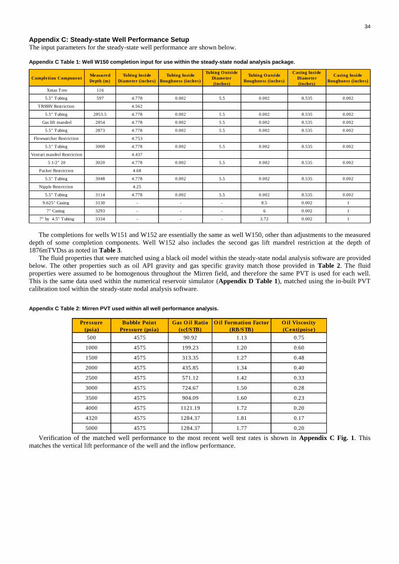
34
Appendix C: Steady-state Well Performance Setup The input parameters for the steady-state well performance are shown below.
Appendix C Table 1: Well W150 completion input for use within the steady-state nodal analysis package.
The completions for wells W151 and W152 are essentially the same as well W150, other than adjustments to the measured
depth of some completion components. Well W152 also includes the second gas lift mandrel restriction at the depth of
1876mTVDss as noted in Table 3.
The fluid properties that were matched using a black oil model within the steady-state nodal analysis software are provided
below. The other properties such as oil API gravity and gas specific gravity match those provided in Table 2. The fluid
properties were assumed to be homogenous throughout the Mirren field, and therefore the same PVT is used for each well.
This is the same data used within the numerical reservoir simulator (Appendix D Table 1), matched using the in-built PVT
calibration tool within the steady-state nodal analysis software.
Appendix C Table 2: Mirren PVT used within all well performance analysis.
Verification of the matched well performance to the most recent well test rates is shown in Appendix C Fig. 1. This
matches the vertical lift performance of the well and the inflow performance.
Completion ComponentMeasured
Depth (m)
Tubing Inside
Diameter (inches)
Tubing Inside
Roughness (inches)
Tubing O utside
Diameter
(inches)
Tubing O utside
Roughness (inches)
Casing Inside
Diameter
(inches)
Casing Inside
Roughness (inches)
Xmas Tree 116
5.5" Tubing 597 4.778 0.002 5.5 0.002 8.535 0.002
TRSSSV Restriction 4.562
5.5" Tubing 2853.5 4.778 0.002 5.5 0.002 8.535 0.002
Gas lift mandrel 2854 4.778 0.002 5.5 0.002 8.535 0.002
5.5" Tubing 2873 4.778 0.002 5.5 0.002 8.535 0.002
Flowwatcher Restriction 4.753
5.5" Tubing 3000 4.778 0.002 5.5 0.002 8.535 0.002
Venturi mandrel Restriction 4.437
5 1/2" 20 3020 4.778 0.002 5.5 0.002 8.535 0.002
Packer Restriction 4.68
5.5" Tubing 3048 4.778 0.002 5.5 0.002 8.535 0.002
Nipple Restriction 4.25
5.5" Tubing 3114 4.778 0.002 5.5 0.002 8.535 0.002
9.625" Casing 3130 - - - 8.5 0.002 1
7" Casing 3293 - - - 6 0.002 1
7" by 4.5" Tubing 3334 - - - 3.72 0.002 1
Pressure
(psia)
Bubble Point
Pressure (psia)
Gas O il Ratio
(scf/STB)
O il Formation Factor
(RB/STB)
O il Viscosity
(Centipoise)
500 4575 90.92 1.13 0.75
1000 4575 199.23 1.20 0.60
1500 4575 313.35 1.27 0.48
2000 4575 435.85 1.34 0.40
2500 4575 571.12 1.42 0.33
3000 4575 724.67 1.50 0.28
3500 4575 904.09 1.60 0.23
4000 4575 1121.19 1.72 0.20
4320 4575 1284.37 1.81 0.17
5000 4575 1284.37 1.77 0.20
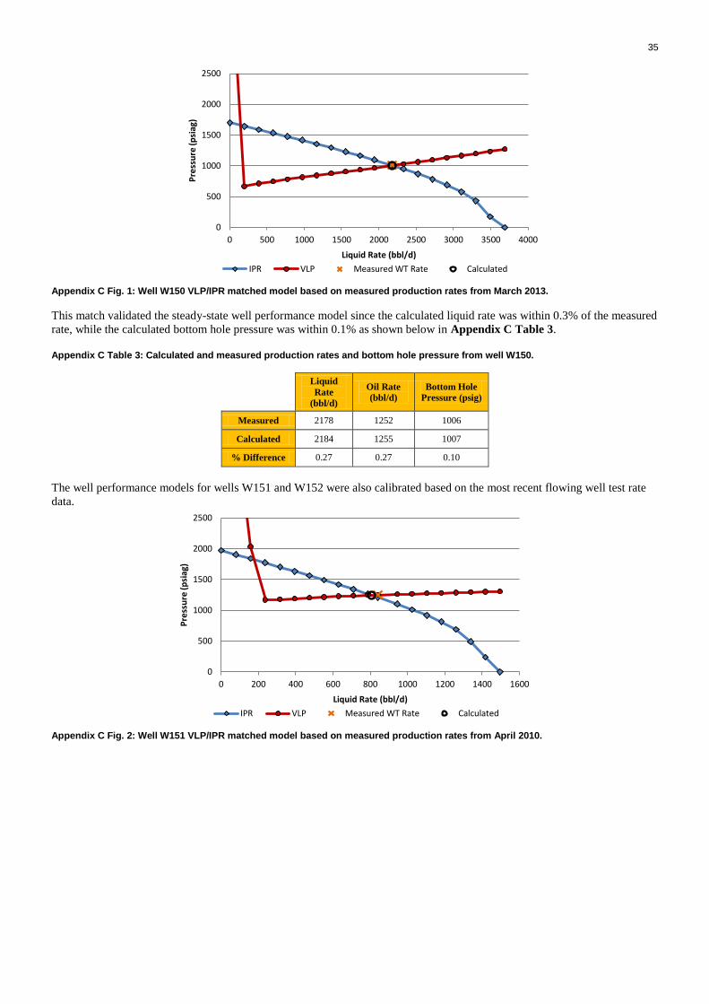
35
Appendix C Fig. 1: Well W150 VLP/IPR matched model based on measured production rates from March 2013.
This match validated the steady-state well performance model since the calculated liquid rate was within 0.3% of the measured
rate, while the calculated bottom hole pressure was within 0.1% as shown below in Appendix C Table 3.
Appendix C Table 3: Calculated and measured production rates and bottom hole pressure from well W150.
Liquid
Rate
(bbl/d)
Oil Rate
(bbl/d)
Bottom Hole
Pressure (psig)
Measured 2178 1252 1006
Calculated 2184 1255 1007
% Difference 0.27 0.27 0.10
The well performance models for wells W151 and W152 were also calibrated based on the most recent flowing well test rate
data.
Appendix C Fig. 2: Well W151 VLP/IPR matched model based on measured production rates from April 2010.
0
500
1000
1500
2000
2500
0 500 1000 1500 2000 2500 3000 3500 4000
Pre
ssu
re (p
siag
)
Liquid Rate (bbl/d)
IPR VLP Measured WT Rate Calculated
0
500
1000
1500
2000
2500
0 200 400 600 800 1000 1200 1400 1600
Pre
ssu
re (p
siag
)
Liquid Rate (bbl/d)
IPR VLP Measured WT Rate Calculated
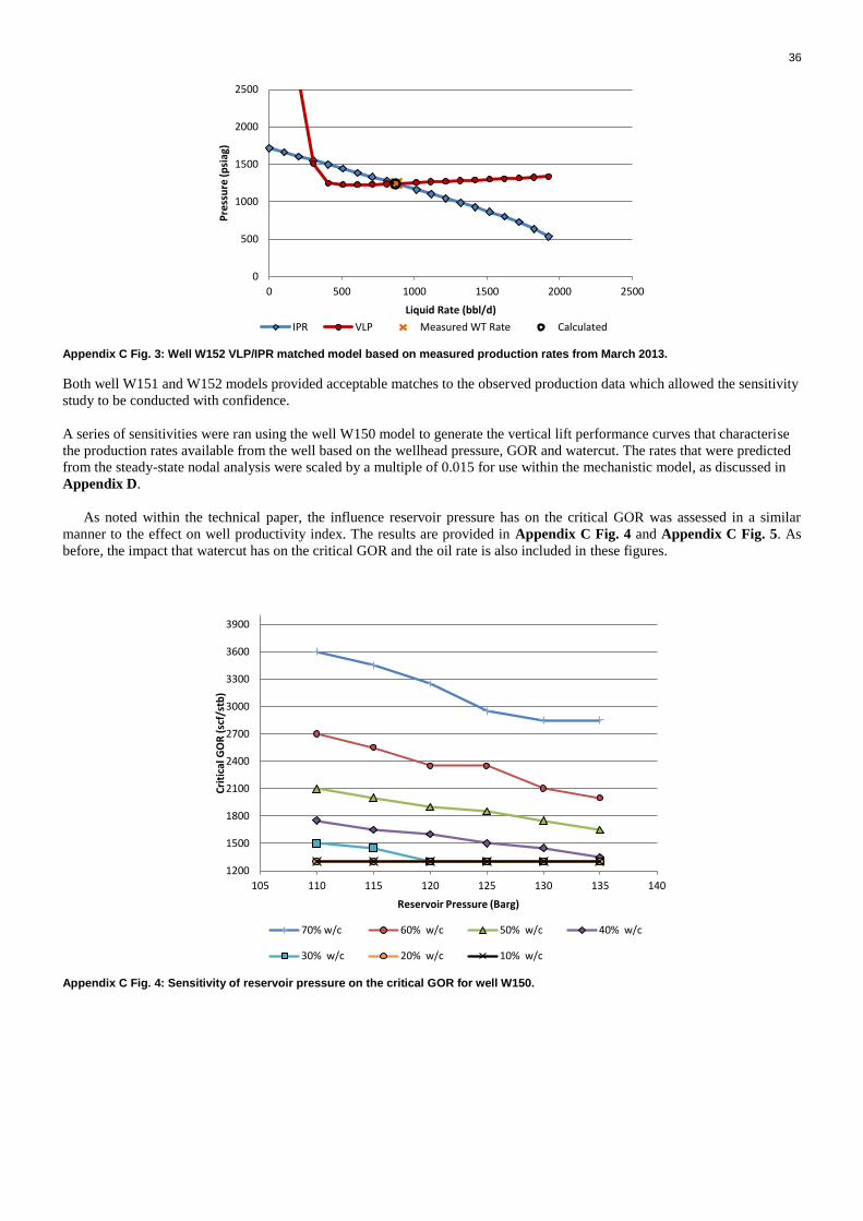
36
Appendix C Fig. 3: Well W152 VLP/IPR matched model based on measured production rates from March 2013.
Both well W151 and W152 models provided acceptable matches to the observed production data which allowed the sensitivity
study to be conducted with confidence.
A series of sensitivities were ran using the well W150 model to generate the vertical lift performance curves that characterise
the production rates available from the well based on the wellhead pressure, GOR and watercut. The rates that were predicted
from the steady-state nodal analysis were scaled by a multiple of 0.015 for use within the mechanistic model, as discussed in
Appendix D.
As noted within the technical paper, the influence reservoir pressure has on the critical GOR was assessed in a similar
manner to the effect on well productivity index. The results are provided in Appendix C Fig. 4 and Appendix C Fig. 5. As
before, the impact that watercut has on the critical GOR and the oil rate is also included in these figures.
Appendix C Fig. 4: Sensitivity of reservoir pressure on the critical GOR for well W150.
0
500
1000
1500
2000
2500
0 500 1000 1500 2000 2500
Pre
ssu
re (p
siag
)
Liquid Rate (bbl/d)
IPR VLP Measured WT Rate Calculated
1200
1500
1800
2100
2400
2700
3000
3300
3600
3900
105 110 115 120 125 130 135 140
Cri
tica
l GO
R (
scf/
stb
)
Reservoir Pressure (Barg)
70% w/c 60% w/c 50% w/c 40% w/c
30% w/c 20% w/c 10% w/c

37
Appendix C Fig. 5: Sensitivity of reservoir pressure on the stable oil production rate at the critical GOR for well W150.
The choking back of Mirren well W150 is being considered to reduce gas production from the field. This would an attempt
to maintain reservoir pressure so that there is enough energy to contribute towards the production of any future infill wells.
Appendix C Fig. 4 shows that maintaining the present reservoir pressure would be beneficial from a well performance point of
view, since further pressure depletion will increase the critical GOR required for stable flow.
There are inherent uncertainties in the values of PI and reservoir pressure used during this analysis. The reasons for this are
twofold. Firstly, the productivity index is a function of rate and pressure. The rates measured on Mirren are back allocated
from by-difference tests that have a wide range of error, mainly due to the low volumes that are produced and the length of
each individual flow test. Secondly, the pressures are uncertain, especially for W150, since it has had no DHPG for many
years of production, and the reservoir pressure is assumed to be equal to that of W152. The above sensitivities show that these
measurement errors and uncertainties have some impact on the critical GOR, but it is minimal. Instead, the biggest contributor
to the critical GOR is the watercut of the well. This is illustrated in Appendix C Fig. 6 and Appendix C Fig. 7. These images
display the same data as Fig. 6 but only for two watercuts. The impact that the increasing the watercut from 40% to 80% has
on the on the oil rate and critical GOR is significant.
0
300
600
900
1200
1500
1800
105 110 115 120 125 130 135 140
Min
imu
m O
il R
ate
(b
bl/
d)
Reservoir Pressure (Bar)
70% w/c 60% w/c 50% w/c 40% w/c
30% w/c 20% w/c 10% w/c
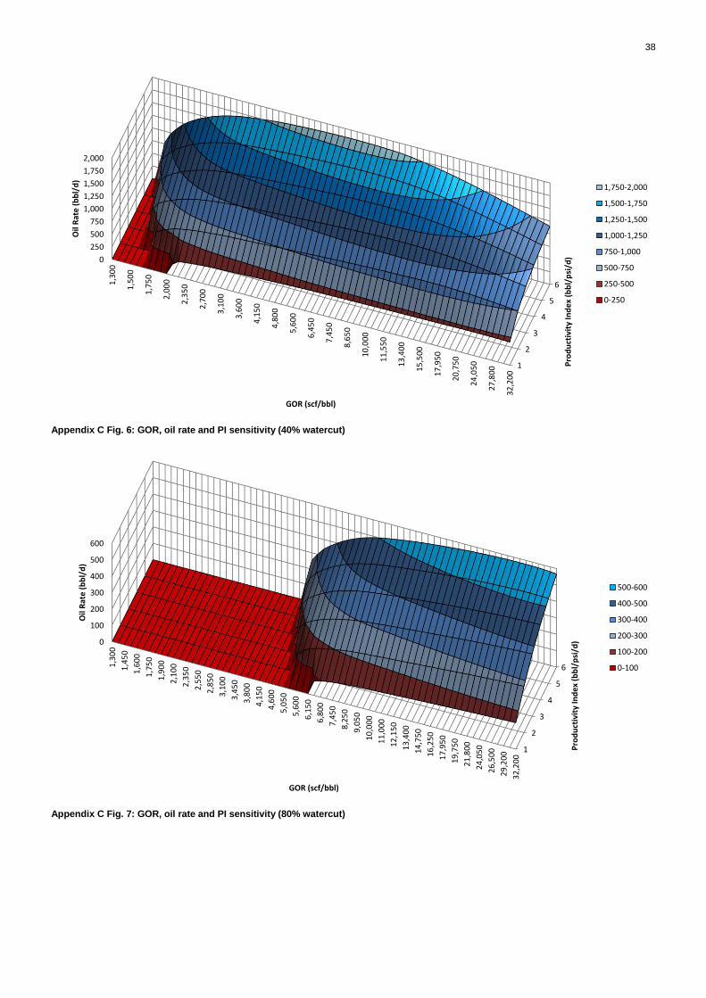
38
Appendix C Fig. 6: GOR, oil rate and PI sensitivity (40% watercut)
Appendix C Fig. 7: GOR, oil rate and PI sensitivity (80% watercut)
1
2
3
4
5
6
0
250
500
750
1,000
1,250
1,500
1,750
2,000
1,3
00
1,5
00
1,7
50
2,0
00
2,3
50
2,7
00
3,1
00
3,6
00
4,1
50
4,8
00
5,6
00
6,4
50
7,4
50
8,6
50
10
,00
0
11
,55
0
13
,40
0
15
,50
0
17
,95
0
20
,75
0
24
,05
0
27
,80
0
32
,20
0
Pro
du
ctiv
ity
Ind
ex
(bb
l/p
si/d
)
Oil
Rat
e (
bb
l/d
)
GOR (scf/bbl)
1,750-2,000
1,500-1,750
1,250-1,500
1,000-1,250
750-1,000
500-750
250-500
0-250
1
2
3
4
5
6
0
100
200
300
400
500
600
1,3
00
1,4
50
1,6
00
1,7
50
1,9
00
2,1
00
2,3
50
2,5
50
2,8
50
3,1
00
3,4
50
3,8
00
4,1
50
4,6
00
5,0
50
5,6
00
6,1
50
6,8
00
7,4
50
8,2
50
9,0
50
10
,00
0
11
,00
0
12
,15
0
13
,40
0
14
,75
0
16
,25
0
17
,95
0
19
,75
0
21
,80
0
24
,05
0
26
,50
0
29
,20
0
32
,20
0
Pro
du
ctiv
ity
Ind
ex
(bb
l/p
si/d
)
Oil
Rat
e (
bb
l/d
)
GOR (scf/bbl)
500-600
400-500
300-400
200-300
100-200
0-100

39
Appendix D: Mechanistic Model Quality Control and History Matching The mechanistic model was quality controlled during the analysis. This included a comparison between the fine and coarse
mechanistic models, and the value of the oil in-place to gas in-place ratio that is observed within the full-field description. The
mechanistic model has a ratio of gas-in place to oil in place of 3.23, while the static description of Mirren has a ratio of 2.85.
This was deemed to be acceptable and the model was then used for the analyses of gas coning. Below the grid.dat file is
attached for reference. This creates the structured grid within the numerical reservoir simulation tool.
MAPBINARY MAPVDB ! Arrays written to map or VDB file MAPOUT ALL RIGHTHANDED ! GRID DEFINITION NX NY NZ 20 1 9 ! GRID DATA ARRAYS ARRAYS DX CON 100 DY CON 100 DZ VALUE 20*130 20*130 20*50 20*30 20*50 20*30 20*100 20*150 20*100 !NTG taken from Mirren Field Static Montage 2012 (Forties=0.33, Lista=0.31, Maureen=0.49) NETGRS VALUE 20*0.33 20*0.33 20*0.33 20*0.31 20*0.31 20*0.31 20*0.49 20*0.49 20*0.49 !Depth taken from Mirren Field Static Montage 2012 (~2500m top salt) !Dip taken from Mirren Summary.ppt, Thomas Harpley September 2011 DEPTH DIP 8200 40 0 LGR CARTREF LGR_1 1 20 1 1 1 9 2 2 2 2 2 2 2 2 2 2 2 2 2 2 2 2 2 2 2 2 1 2 2 2 2 2 2 2 2 2 ENDREF ENDLGR !POROSITY taken from Mirren Field Static Montage 2012 (Forties=0.2, Lista=0.215, Maureen=0.22) POROSITY VALUE 20*0.2 20*0.2 20*0.2 20*0.215 20*0.215 20*0.215 20*0.22 20*0.22 20*0.22 !Permeabilities taken from Mirren Field Static Montage 2012 (Field average 10mD) KX CON 15 KY CON 15 KZ MULT 0.1 KX IEQUIL CON 1 IREGION CON 1 IRELPM CON 1 INFLUX 1 IINF JINF KINF SINF GRID LGR_1 WINDOW 40 40 1 1 1 18 XCALC ENDAQ
The coarse grid model has the same root grid as the above grid.dat file that generates the fine grid, simply with the
omission of the local grid refinement. The well is located in cell 132:1:31 and 13:1:5 within the fine and coarse grid models
respectively. This results in a standoff to the gas oil contact of 92m, as required (Table 3). The Black Oil PVT model data
used within the numerical simulation software package is provided in Appendix D Table 1.

40
Appendix D Table 1: Mirren Black Oil PVT data used within numerical reservoir simulation model.
Appendix D Table 2: Mirren water properties.
Water
Density
(lb/ft3)
Water
Compressibility
(1/psia)
Water
Viscosity
(Centipoise)
Water Formation Volume Factor
[At initial datum reservoir
pressure]
Datum Pressure for
Water Compressibility
(psia)
65.5 3.50E-06 0.5 1.04 4100
Once the numerical grid was created it could be propagated with the fluid data provided above. A quality control of the
mechanistic model grid was then conducted to ensure the fine and coarse grid models were comparable.
Appendix D Table 3: Grid volumetric quality control
Oil in Place (Mstb) Gas in place (MMscf) Water in place (Mstb)
Coarse 452 1455 829
Fine 448 1455 832
% Difference 0.10 -0.05 -0.27
A good match between the coarse and fine grid mechanistic model volumes was obtained. The volumes within the
mechanistic model are representative of 1/150th
of Mirren’s total in-place oil. As such, the cumulative volumes produced by
well W150 within the mechanistic model required scaling. The production rates of oil, water and gas were scaled by a
multiplier of 0.015. This allowed an acceptable match on field recorded reservoir pressure decline using the mechanistic
models, as shown below in Appendix D Fig. 1. The same scaling factor was used to adjust the production rates that were
predicted by the vertical lift performance curves.
Pressure
(psia)
Gas Oil Ratio
(Mscf/STB)
Oil Formation Volume
Factor (STB/RB)
Gas Formation Volume
Factor (Scf/RB)
Oil Viscosity
(Centipoise)
Gas Viscosity
(Centipoise)
6500 2.6652 2.459 0.632 0.0814 0.0517
6000 2.2762 2.264 0.658 0.1015 0.046
5500 1.9274 2.089 0.689 0.1227 0.0407
5000 1.6189 1.934 0.728 0.1446 0.036
4750 1.4797 1.865 0.751 0.1557 0.0338
4575.87 1.3886 1.819 0.769 0.1635 0.0324
4446.1 1.324 1.786 0.784 0.1692 0.0313
4072 1.1527 1.7 0.837 0.187 0.0285
3721.5 1.0089 1.628 0.9 0.2058 0.0262
3500 0.925 1.586 0.947 0.219 0.0248
3250 0.8359 1.54 1.011 0.2351 0.0233
3000 0.7522 1.498 1.087 0.2528 0.0219
2750 0.6733 1.458 1.18 0.2723 0.0206
2500 0.5988 1.419 1.293 0.2939 0.0195
2250 0.5281 1.383 1.435 0.3176 0.0185
2000 0.461 1.348 1.615 0.344 0.0175
1750 0.3971 1.314 1.851 0.3733 0.0167
1500 0.3361 1.282 2.17 0.4059 0.016
1250 0.2777 1.251 2.622 0.4423 0.0154
1000 0.2215 1.22 3.306 0.4834 0.0148
750 0.1669 1.19 4.456 0.5303 0.0143
500 0.1129 1.159 6.77 0.586 0.0137
250 0.0536 1.123 13.752 0.6616 0.0129
14.7 0 1.072 238.488 0.8857 0.01
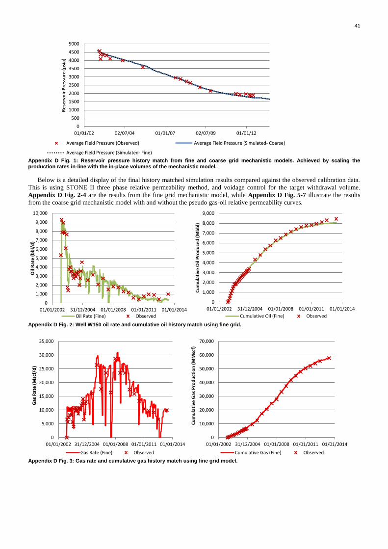
41
Appendix D Fig. 1: Reservoir pressure history match from fine and coarse grid mechanistic models. Achieved by scaling the production rates in-line with the in-place volumes of the mechanistic model.
Below is a detailed display of the final history matched simulation results compared against the observed calibration data.
This is using STONE II three phase relative permeability method, and voidage control for the target withdrawal volume.
Appendix D Fig. 2-4 are the results from the fine grid mechanistic model, while Appendix D Fig. 5-7 illustrate the results
from the coarse grid mechanistic model with and without the pseudo gas-oil relative permeability curves.
Appendix D Fig. 2: Well W150 oil rate and cumulative oil history match using fine grid.
Appendix D Fig. 3: Gas rate and cumulative gas history match using fine grid model.
0
500
1000
1500
2000
2500
3000
3500
4000
4500
5000
01/01/02 02/07/04 01/01/07 02/07/09 01/01/12
Re
serv
oir
Pre
ssu
re (p
sia)
Average Field Pressure (Observed) Average Field Pressure (Simulated- Coarse)
Average Field Pressure (Simulated- Fine)
0
1,000
2,000
3,000
4,000
5,000
6,000
7,000
8,000
9,000
10,000
01/01/2002 31/12/2004 01/01/2008 01/01/2011 01/01/2014
Oil
Rat
e (
bb
l/d
)
Oil Rate (Fine) Observed
0
1,000
2,000
3,000
4,000
5,000
6,000
7,000
8,000
9,000
01/01/2002 31/12/2004 01/01/2008 01/01/2011 01/01/2014
Cu
mu
lati
ve O
il P
rod
uce
d (
Mb
bl)
Cumulative Oil (Fine) Observed
0
5,000
10,000
15,000
20,000
25,000
30,000
35,000
01/01/2002 31/12/2004 01/01/2008 01/01/2011 01/01/2014
Gas
Rat
e (
Msc
f/d
)
Gas Rate (Fine) Observed
0
10,000
20,000
30,000
40,000
50,000
60,000
70,000
01/01/2002 31/12/2004 01/01/2008 01/01/2011 01/01/2014
Cu
mu
lati
ve G
as P
rod
uct
ion
(M
Msc
f)
Cumulative Gas (Fine) Observed

42
Appendix D Fig. 4: Water rate and cumulative water history match using fine grid model.
Appendix D Fig. 5: Oil rate and cumulative oil history matching using coarse grid model (Original gas-oil relative permeability and pseudo relative permeability).
Appendix D Fig. 6: Gas rate and cumulative gas history matching using coarse grid model (Original gas-oil relative permeability and pseudo relative permeability).
0
200
400
600
800
1000
1200
1400
01/01/2002 31/12/2004 01/01/2008 01/01/2011 01/01/2014
Wat
er
Rat
e (
bb
l/d
)
Water Rate (Fine) Observed
0
100
200
300
400
500
600
01/01/2002 31/12/2004 01/01/2008 01/01/2011 01/01/2014
Cu
mu
lati
ve W
ate
r P
rod
uct
ion
(M
bb
l)
Cumulative Water (Fine) Observed
0
2,000
4,000
6,000
8,000
10,000
01/01/2002 31/12/2004 01/01/2008 01/01/2011 01/01/2014
Oil
Rat
e (
bb
l/d
)
Oil Rate (Coarse Sgcrit=3%)Oil Rate (Coarse Sgcrit=7%)Observed
0
2,000
4,000
6,000
8,000
10,000
01/01/2002 31/12/2004 01/01/2008 01/01/2011 01/01/2014
Cu
mu
lati
ve O
il P
rod
uce
d (
Mb
bl)
Cumulative Oil (Coarse Sgcrit=3%)Cumulative Oil (Coarse Sgcrit=7%)Observed
0
5,000
10,000
15,000
20,000
25,000
30,000
35,000
01/01/2002 31/12/2004 01/01/2008 01/01/2011 01/01/2014
Gas
Rat
e (
Msc
f/d
)
Gas Rate (Coarse Sgcrit=3%)Gas Rate (Coarse Sgcrit=7%)Observed
0
10,000
20,000
30,000
40,000
50,000
60,000
70,000
01/01/2002 31/12/2004 01/01/2008 01/01/2011 01/01/2014
Cu
mu
lati
ve G
as P
rod
uct
ion
(M
Msc
f)
Cumulative Gas (Coarse Sgcrit=3%)Cumulative Gas (Coarse Sgcrit=7%)Observed

43
Appendix D Fig. 7: Water rate and cumulative water history matching using coarse grid model (Original gas-oil relative permeability and pseudo relative permeability).
Appendix D Fig. 8: GOR and watercut history match from fine and coarse grid (Sgcrit=7%) simulation models.
It is understood that the increased GOR during the simulation illustrated in Appendix D Fig. 8 above the observed GOR
from W150 is partially responsible for the optimistic recovery times that are displayed within Fig. 15 when compared to field
observed recovery times. The other factor that plays into the quality of the simulated recovery when compared against the field
observed data is the inherent uncertainty within the field observations. As a means of estimating what reservoir behaviour
would be required to match the field observed recovery time, the results from the relative GOR contour map were used to back
calculate the relative GOR required to match the observed 2012 recovery time. It was found that to match the observed
response the critical GOR would have had to have been 7500scf/bbl for well W150. This could be possible, but only if there
was a vast change watercut of the well. It was found from the sensitivity analysis (Fig. 7) that if W150 had an 83% watercut
with the present productivity index of 3.6bbl/day/psi, the critical GOR would be roughly 7500scf/bbl. The watercut was
therefore increased so that the critical GOR rose to 7500scf/bbl. The pre-shut-in GOR was set to 10,000scf/bbl which is the
present producing GOR of well W150. When analysis was completed the simulated recovery time matched the field observed
data, as illustrated in Appendix D Fig. 9.
0
200
400
600
800
1000
1200
01/01/2002 31/12/2004 01/01/2008 01/01/2011 01/01/2014
Wat
er
Rat
e (
bb
l/d
)
Water Rate (Coarse Sgcrit=3%)
Water Rate (Coarse Sgcrit=7%)
Observed
0
100
200
300
400
500
600
01/01/2002 31/12/2004 01/01/2008 01/01/2011 01/01/2014
Cu
mu
lati
ve W
ate
r P
rod
uct
ion
(M
bb
l)
Cumulative Water (Coarse Sgrit=3%)Cumulative Water (Coarse Sgrit=7%)Observed
0
5,000
10,000
15,000
20,000
25,000
30,000
35,000
01/01/2002 31/12/2004 01/01/2008 01/01/2011 01/01/2014
GO
R (
scf/
STB
)
GOR (Coarse Sgcrit=7%) GOR (Fine) Observed
0.0
0.2
0.4
0.6
0.8
1.0
01/01/2002 31/12/2004 01/01/2008 01/01/2011 01/01/2014
Wat
erc
ut
(Fra
ctio
n)
Watercut (Coarse Sgcrit=7%)Watercut (Fine)Observed
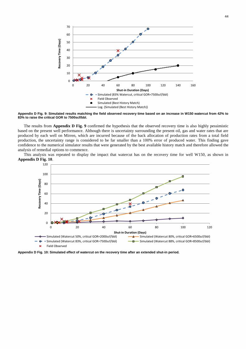
44
Appendix D Fig. 9: Simulated results matching the field observed recovery time based on an increase in W150 watercut from 42% to 83% to raise the critical GOR to 7500scf/bbl.
The results from Appendix D Fig. 9 confirmed the hypothesis that the observed recovery time is also highly pessimistic
based on the present well performance. Although there is uncertainty surrounding the present oil, gas and water rates that are
produced by each well on Mirren, which are incurred because of the back allocation of production rates from a total field
production, the uncertainty range is considered to be far smaller than a 100% error of produced water. This finding gave
confidence to the numerical simulator results that were generated by the best available history match and therefore allowed the
analysis of remedial options to commence.
This analysis was repeated to display the impact that watercut has on the recovery time for well W150, as shown in
Appendix D Fig. 10.
Appendix D Fig. 10: Simulated effect of watercut on the recovery time after an extended shut-in period.
0
10
20
30
40
50
60
70
0 20 40 60 80 100 120 140 160
Re
cove
ry T
ime
(D
ays)
Shut-in Duration (Days)
Simulated (83% Watercut, critical GOR=7500scf/bbl)Field Observed
Simulated (Best History Match)Log. (Simulated (Best History Match))
0
20
40
60
80
100
120
0 20 40 60 80 100 120
Re
cove
ry T
ime
(D
ays)
Shut-in Duration (Days) Simulated (Watercut 50%, critical GOR=2000scf/bbl) Simulated (Watercut 80%, critical GOR=6500scf/bbl)
Simulated (Watercut 83%, critical GOR=7500scf/bbl) Simulated (Watercut 88%, critical GOR=8500scf/bbl)
Field Observed
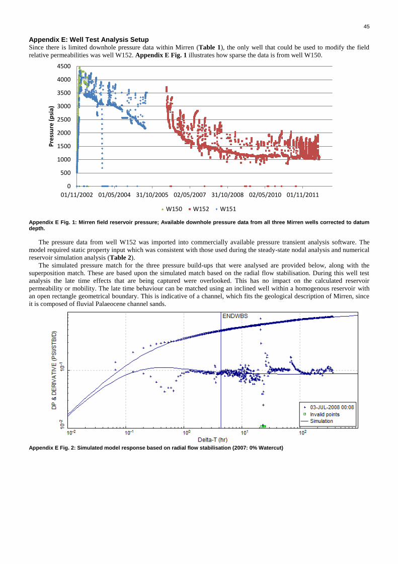
45
Appendix E: Well Test Analysis Setup Since there is limited downhole pressure data within Mirren (Table 1), the only well that could be used to modify the field
relative permeabilities was well W152. Appendix E Fig. 1 illustrates how sparse the data is from well W150.
Appendix E Fig. 1: Mirren field reservoir pressure; Available downhole pressure data from all three Mirren wells corrected to datum depth.
The pressure data from well W152 was imported into commercially available pressure transient analysis software. The
model required static property input which was consistent with those used during the steady-state nodal analysis and numerical
reservoir simulation analysis (Table 2).
The simulated pressure match for the three pressure build-ups that were analysed are provided below, along with the
superposition match. These are based upon the simulated match based on the radial flow stabilisation. During this well test
analysis the late time effects that are being captured were overlooked. This has no impact on the calculated reservoir
permeability or mobility. The late time behaviour can be matched using an inclined well within a homogenous reservoir with
an open rectangle geometrical boundary. This is indicative of a channel, which fits the geological description of Mirren, since
it is composed of fluvial Palaeocene channel sands.
Appendix E Fig. 2: Simulated model response based on radial flow stabilisation (2007: 0% Watercut)
0
500
1000
1500
2000
2500
3000
3500
4000
4500
01/11/2002 01/05/2004 31/10/2005 02/05/2007 31/10/2008 02/05/2010 01/11/2011
Pre
ssu
re (
psi
a)
W150 W152 W151

46
Appendix E Fig. 3: 2007 Pressure match using simulated model.
Appendix E Fig. 4: 2007 Superposition match.
Appendix E Fig. 5: Simulated model response based on radial flow stabilisation (2008: 15% Watercut)

47
Appendix E Fig. 6: 2008 Pressure match using simulated model.
Appendix E Fig. 7: 2008 Superposition match.
Appendix E Fig. 8: Simulated model response based on radial flow stabilisation (2012: 54% Watercut)
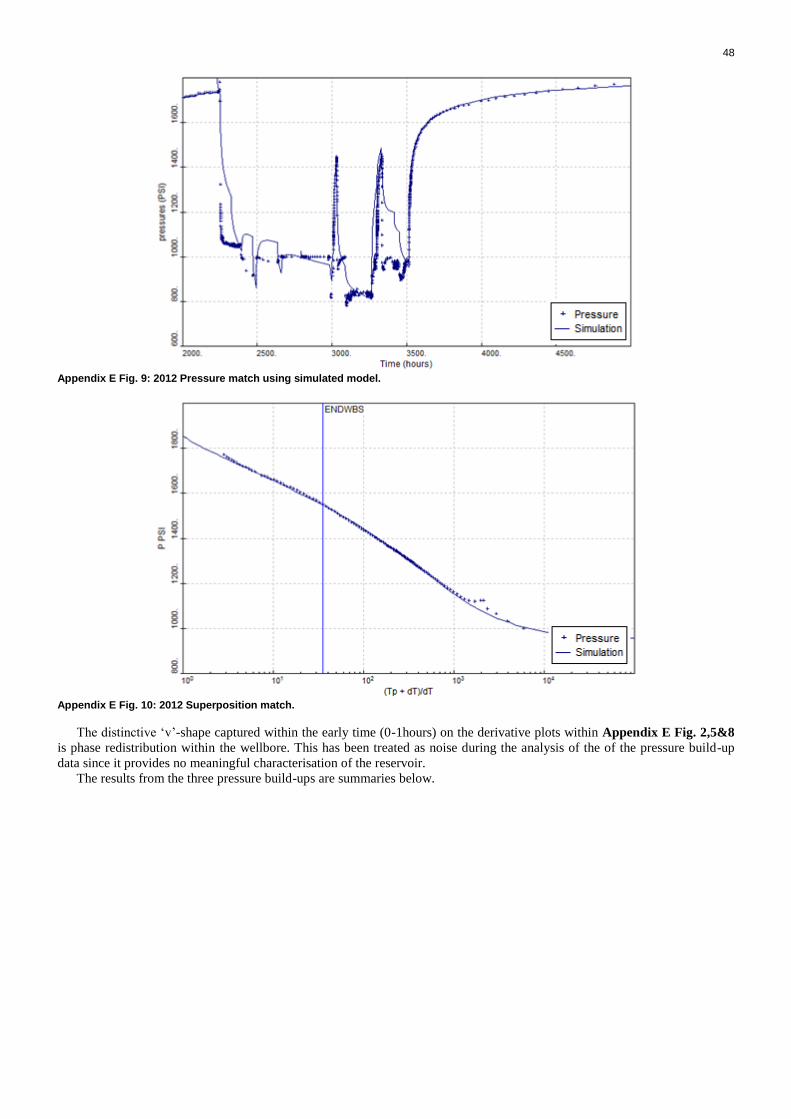
48
Appendix E Fig. 9: 2012 Pressure match using simulated model.
Appendix E Fig. 10: 2012 Superposition match.
The distinctive ‘v’-shape captured within the early time (0-1hours) on the derivative plots within Appendix E Fig. 2,5&8
is phase redistribution within the wellbore. This has been treated as noise during the analysis of the of the pressure build-up
data since it provides no meaningful characterisation of the reservoir.
The results from the three pressure build-ups are summaries below.

49
Appendix E Table 1: Well test analysis parameter results.
W152 Well Test Analysis Results
Test Date 2007 2008 2012
Wellbore Storage, STB/psi 0.05 0.03 0.52
Skin (mech) -0.9 -0.8 -2.2
Permeability, mD 0.49 0.26 0.21
Areal ky/kx 1 1 1
Kv/Kh 0.77 0.75 0.76
Drainage Length/2, ft 737.5 737.5 737.5
Zp/Heff 0.50 0.50 0.50
Deviation, degrees 40 40 40
Azimuth, degrees 0 0 0
Skin (Global) -2.1 -2.1 -3.1
Skin (Geometrical) -1.4 -1.4 -1.4
Permeability Thickness, mD.ft 560 297 243
Initial Pressure, psi 2812 2479 1855
The observed reduction in krh was included using Eq.1-4 and resulted in the adaptation of the normalised relative
permeability of the analog curves. The results of the relative permeability modifications are shown in Appendix E Table 2. Appendix E Table 2: Results from iterative method to calculate water saturations and relative permeabilities based on the watercut and normalised mobility thickness observed during well test analysis.
Date Water Cut
(%)
Fractional
Flow, fw
Mobility Thickness
[Well Test] (mD-
feet)
Normalised Relative
Mobility Sw Kro Krw
01/07/2007 0 0.00 560 1.00 0.25 1.00 0.00
03/07/2008 15 0.11 300 0.53 0.46 0.18 0.03
31/07/2012 54 0.45 240 0.44 0.53 0.09 0.10
50
Appendix F: Material Balance Study The pressure depletion of 800psi that was observed when well W152 was brought online 4years after production commenced
on Mirren was a clear sign that there is significant pressure communication (Appendix E Fig. 1). However, uncertainties
surrounding the present reservoir pressure due to the lack of down hole pressure data for two of the wells (W150 and W151)
indicated the need for further analysis. The analytical material balance method was applied to define whether the assumption
that the extrapolated pressure at the end of pressure build-ups on well W152 is a fair representation of the average reservoir
pressure. The same produced volumes were used within the material balance analysis as the numerical reservoir simulation
study. The pressure data was adjusted to datum depth from the raw readings displayed in Appendix E Fig. 1.
Appendix F Fig. 1: Three tank Mirren material balance representation.
A simple three-tank material balance model was created with the in-place Mirren volumes divided evenly between each
tank. It was found that using the entire in-place oil and gas volumes resulted in an excess of pressure support in all three wells.
By reducing the connectivity of the gas cap (modelled through lowering the gas cap volume), a fair match to the initial
pressure decline on well W150 could be made, yet the pressure within the other two tanks was still significantly higher than
measured. A more complex material balance model was created to include distant oil volumes. These provide weak pressure
support to the three producing wells. These distant tanks were connected via transmissible connections which could be
visualised as baffles within the reservoir. This model could be history matched against the available pressure data from the
three wells, as show in Appendix F Fig. 2.
STOIIP and GIIP split evenly,
giving GIIP/STOIIP = 1.8
STOIIP: 61.6MMstb
GIIP: 110Bscf
W150: Too much energy
01/11/2002 03/04/2005 04/09/2007 04/02/2010 08/07/2012
0
1500
3000
4500
6000
Production Simulation - Mirren
Time (date d/m/y)
Tank Pressure (psia)
Tank Pressure
W150 : History
W150 : Simulation
01/11/2002 03/04/2005 04/09/2007 04/02/2010 08/07/2012
3200
3600
4000
4400
4800
Production Simulation - Mirren
Time (date d/m/y)
Tank Pressure (psia)
Tank Pressure
W151 : History
W151 : Simulation
01/11/2002 03/04/2005 04/09/2007 04/02/2010 08/07/2012
1000
2000
3000
4000
5000
Production Simulation - Mirren
Time (date d/m/y)
Tank Pressure (psia)
Tank Pressure
W152 : History
W152 : Simulation
W151: Too much energy
W152: Too much energy
51
Appendix F Fig. 2: Six tank Mirren material balance representation.
Since the material balance technique produces in non-unique results an alternative history match was achieved by lowering
the connected gas volume and introducing a greater amount of aquifer support into the western well, W150. The results of this
alternative history match are shown in Appendix F Fig. 3.
STOIIP and GIIP split by expected
recovery factor. Southern tank
included, containing remainder from STOIIP.
STOIIP: 65.9MMstb GIIP: 149.8Bscf
W150: Good history match
W151: Good history match
W152: Good history match
01/11/2002 03/04/2005 04/09/2007 04/02/2010 08/07/2012
1000
2000
3000
4000
5000
Production Simulation - Mirren
Time (date d/m/y)
Tank Pressure (psia)
Tank Pressure
W152 : History
W152 : Simulation
01/11/2002 03/04/2005 04/09/2007 04/02/2010 08/07/2012
1000
2000
3000
4000
5000
Production Simulation - Mirren
Time (date d/m/y)
Tank Pressure (psia)
Tank Pressure
W150 : History
W150 : Simulation
01/11/2002 03/04/2005 04/09/2007 04/02/2010 08/07/2012
2250
3000
3750
4500
5250
Production Simulation - Mirren
Time (date d/m/y)
Tank Pressure (psia)
Tank Pressure
W151 : History
W151 : Simulation
52
Appendix F Fig. 3: Six tank Mirren material balance representation with additional aquifer support on well W150.
The material balance method allowed the available pressure data to be matched based on the cumulative produced
volumes. The reservoir pressure within the two wells that presently do not have downhole pressure gauges could also be
estimated using this method. The range reservoir pressure across the material balance model was 800psi. Between the south
and west of the field, which are understood to have lower aquifer connectivity (based on later water breakthrough), the
reservoir pressure is within 400psi. The region modelled here as the south of the field also saw significant amount of pressure
depletion without any producing well assigned to it. By the end of the history the pressure within the southern tank is 60psi
higher than the measured pressure from well W152. The pressure decline for each tank can be observed in Appendix F Fig. 4.
These results were taken to validate the assumption that the measured bottom hole pressure from well W152 is a fair
representation of the field average reservoir pressure when extrapolated to estimate field average reservoir pressure. The
calculated reservoir pressure from well W152 was used as the field reservoir pressure throughout the remainder of the analysis.
STOIIP and GIIP split by expected
recovery factor. Southern tank
included, containing remainder from STOIIP.
STOIIP: 69.7MMstb GIIP: 128Bscf
W150: Good history match
W151: Good history match
W152: Good history match
01/11/2002 03/04/2005 04/09/2007 04/02/2010 08/07/2012
1000
2000
3000
4000
5000
Production Simulation - Mirren
Time (date d/m/y)
Tank Pressure (psia)
Tank Pressure
W152 : History
W152 : Simulation
01/11/2002 03/04/2005 04/09/2007 04/02/2010 08/07/2012
2000
3000
4000
5000
6000
Production Simulation - Mirren
Time (date d/m/y)
Tank Pressure (psia)
Tank Pressure
W151 : History
W151 : Simulation
01/11/2002 03/04/2005 04/09/2007 04/02/2010 08/07/2012
1000
2000
3000
4000
5000
Production Simulation - Mirren
Time (date d/m/y)
Tank Pressure (psia)
Tank Pressure
W150 : History
W150 : Simulation
53
Appendix F Fig. 4: Reservoir pressure estimation including wells W150, W151, W152, field average pressure and unproduced southern volume.
0
500
1000
1500
2000
2500
3000
3500
4000
4500
5000
30/12/2001 30/12/2004 31/12/2007 30/12/2010 30/12/2013
Pre
ssu
re (
psi
a)
W150 W152 W151 South Field
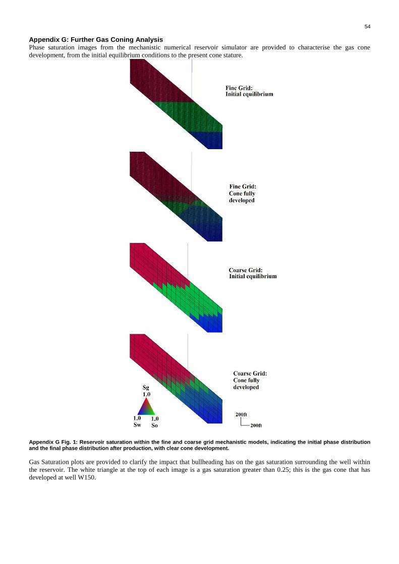
54
Appendix G: Further Gas Coning Analysis Phase saturation images from the mechanistic numerical reservoir simulator are provided to characterise the gas cone
development, from the initial equilibrium conditions to the present cone stature.
Appendix G Fig. 1: Reservoir saturation within the fine and coarse grid mechanistic models, indicating the initial phase distribution and the final phase distribution after production, with clear cone development.
Gas Saturation plots are provided to clarify the impact that bullheading has on the gas saturation surrounding the well within
the reservoir. The white triangle at the top of each image is a gas saturation greater than 0.25; this is the gas cone that has
developed at well W150.

55
Appendix G Fig. 2: Gas saturation surrounding near wellbore region of the fine grid mechanistic model during bullheading and when producing with the support of gas lift after a 60day shut-in period.
Appendix G Fig. 2 (left column) illustrates the increase in gas saturation within the reservoir around the perforation where
the gas is injected. This gas is available during restart, allowing production to commence more readily a higher rate, since the
pressure drop within the well has been reduced through a reduction in gravitational head. Since the well is producing at a
higher rate, the gas cone redevelops more quickly, providing the free gas required for stable well performance. Appendix G
Fig. 2 (right column) illustrates how the grid block that contains the well perforation has a gas saturation of 0.05. This is after
a 60day shut-in, and the gas cone has relaxed from the near wellbore region, resulting in a 90% drop in free gas surrounding
the well. The first 2.5days of production with the aid of gas lift results in only a slight change in gas saturation from 0.05 to
0.10 within the grid block that contains the well.

56
Ramp-up Procedure
Appendix G Fig. 3: Well W150 ramp-up rate after various shut-in periods, with and without bullheading.
Appendix G Fig. 3 indicates that bullheading can allow the initial oil rate after the shut-in to be raised. However, once the
injected gas surrounding the near wellbore region has been produced the rates decline. This dip signals the production of the
oil and water with a lower gas rate, prior to gas cone redevelopment. Here the bullheading injection rate and duration was not
adjusted to account for the shut-in duration. As such, for a longer shut-in period the increase in oil rate is short-lived; the rates
decline until the gas cone begins to redevelop. These results suggest that for longer shut-in periods a greater volume of gas
could be bullheaded into the reservoir to extend the period with increased production rates. This is clearly limited by
availability of gas lift rate and supply pressure. Significantly increasing the bullheading duration is unfavourable since the gas
cone continues to relax while the bullheading takes place.
A result of this behaviour means the cumulative volumes produced after restarting the well can be improved through
bullheading. For instance, bullheading 2MMscf/d into the reservoir for two days after a 50day shut-in has increased the
cumulative oil production over a 14day recovery period by 26%. However, the same bullheading operation implemented after
a 10day or 100day shut-in does change the cumulative oil produced. Therefore, optimisation would be required to quantify the
desired rate and duration of bullheading for individual shut-in periods. Based on this work the effect that bullheading has on
the oil recovery rates were positive but complex. To highlight the positive benefit that bullheading can have the field
production rates were assessed, as shown in Fig. 17b since it was clear that by advancing the restart of well W152 the total
field production rates could be increased.
The effect of bullheading well W150 for two days prior to bullheading well W152 for two days was assessed. The results
of the field cumulative oil produced after restart and the field oil rate are compared against the results shown in Fig. 17b are
provided below in Appendix G Fig. 4.
0
10,000
20,000
30,000
40,000
50,000
60,000
70,000
80,000
0
200
400
600
800
1000
1200
1400
1600
0 10 20 30 40 50 60
Cu
mu
lati
ve O
il P
rod
uce
d a
fte
r R
est
art
(bb
l)
Oil
Rat
e (
bb
l/d
)
Recovery (Days)
10 Day Shut-in (Gas lift Rate) 10 Day Shut-in (Bullhead Rate) 50 Day Shut-in (Bullhead Rate)
50 Day Shut-in (Gas lift Rate) 100 Day Shut-in (Bullhead Rate) 100 Day Shut-in (Gas lift Rate)
10 Day Shut-in (Gas lift Cum.) 10 Day Shut-in (Bullhead Cum.) 50 Day Shut-in (Bullhead Cum.)
50 Day Shut-in (Gas lift Cum.) 100 Day Shut-in (Bullhead Cum.) 100 Day Shut-in (Gas lift Cum.)
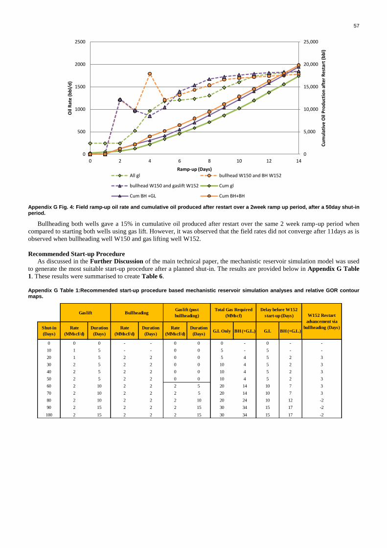
57
Appendix G Fig. 4: Field ramp-up oil rate and cumulative oil produced after restart over a 2week ramp up period, after a 50day shut-in period.
Bullheading both wells gave a 15% in cumulative oil produced after restart over the same 2 week ramp-up period when
compared to starting both wells using gas lift. However, it was observed that the field rates did not converge after 11days as is
observed when bullheading well W150 and gas lifting well W152.
Recommended Start-up Procedure
As discussed in the Further Discussion of the main technical paper, the mechanistic reservoir simulation model was used
to generate the most suitable start-up procedure after a planned shut-in. The results are provided below in Appendix G Table
1. These results were summarised to create Table 6.
Appendix G Table 1:Recommended start-up procedure based mechanistic reservoir simulation analyses and relative GOR contour maps.
0
5,000
10,000
15,000
20,000
25,000
0
500
1000
1500
2000
2500
0 2 4 6 8 10 12 14
Cu
mu
lati
ve O
il P
rod
uct
ion
aft
er
Re
star
t (b
bl)
Oil
Rat
e (
bb
l/d
)
Ramp-up (Days) All gl bullhead W150 and BH W152
bullhead W150 and gaslift W152 Cum gl
Cum BH +GL Cum BH+BH
Shut-in
(Days)
Rate
(MMscf/d)
Duration
(Days)
Rate
(MMscf/d)
Duration
(Days)
Rate
(MMscf/d)
Duration
(Days)G.L Only BH (+G.L.) G.L BH (+G.L.)
0 0 0 - - 0 0 0 - 0 - -
10 1 5 - - 0 0 5 - 5 - -
20 1 5 2 2 0 0 5 4 5 2 3
30 2 5 2 2 0 0 10 4 5 2 3
40 2 5 2 2 0 0 10 4 5 2 3
50 2 5 2 2 0 0 10 4 5 2 3
60 2 10 2 2 2 5 20 14 10 7 3
70 2 10 2 2 2 5 20 14 10 7 3
80 2 10 2 2 2 10 20 24 10 12 -2
90 2 15 2 2 2 15 30 34 15 17 -2
100 2 15 2 2 2 15 30 34 15 17 -2
Total Gas Required
(MMscf)
Gaslift (post
bullheading) W152 Restart
advancement via
bullheading (Days)
Delay before W152
start-up (Days)Gaslift Bullheading

58
Appendix H: Computer Software Commercially available software has been used throughout this project. The methods used within each program have been
clearly defined within the main body of the text, notably in the Analysis Tools section. The specific software that has been
used during each individual section is provided below.
Steady-state well performance
Petroleum Experts, IPM Toolkit: Prosper version 8.1
http://www.petex.com/products/
Material Balance
Petroleum Experts, IPM Toolkit: MBAL version 8.1
http://www.petex.com/products/
Well test analysis
Well Test Solutions, PIE Well-Test Software
http://www.welltestsolutions.com/
Numerical reservoir simulator
Halliburton Landmark Software and Services, Nexus Reservoir Simulation
https://www.landmarksoftware.com/Pages/Nexus.aspx