Embed Size (px)
Citation preview

1
IMPACTS OF EXHCHANGE RATE ON TERMS OF TRADE AND VOLUME OF TRADE
YOUNGJAE LEE
Department of Agricultural Economics and Agribusiness Louisiana State University AgCenter
101 Agricultural Administration Building Baton Rouge LA 70803-5606
Phone: 225-578-2754 Fax: 225-578-2716
E-Mail: [email protected]
P. LYNN KENNEDY
Department of Agricultural Economics and Agribusiness Louisiana State University AgCenter
101 Agricultural Administration Building Baton Rouge LA 70803-5606
Phone: 225-578-2726 Fax: 225-578-2716
E-Mail: [email protected]
Selected Paper prepared for presentation at the Southern Agricultural Economics Association Annual Meeting, Atlanta, Georgia, January 31-February 3, 2009
Copyright 2009 by Youngjae Lee and P. Lynn Kennedy. All rights reserved. Readers may make verbatim copies of this document for non-commercial purposes by any means, provided that this copyright notice appears on all such copies.
2
IMPACTS OF EXHCHANGE RATE ON TERMS OF TRADE AND VOLUME OF TRADE
ABSTRACT
Direct and indirect effects of exchange rates on foreign and home prices may induce a change in terms of trade and volume of trade. In particular, the price effect in substitutability between foreign and home products and endogeneity of the foreign price provide evidence for the indirect impact of the exchange rate on home price. Furthermore, elasticity of substitution and degree of returns to scale influence the impact of the exchange rate on terms of trade and trade volume. In an empirical examination of the Korean beef market, this study found a decrease in terms of trade and an increase in volume of trade when the U.S. dollar depreciates, and an increase in terms of trade and a decrease in volume of trade when the U.S. dollar appreciates. However, the effect on terms of trade is greater than the effect on volume, implying that the foreign price elasticity of import demand is less than one.
Key words: exchange rate, home and foreign prices, direct and indirect effects, terms of trade, volume of trade.
The study of the exchange rate in international commodity trade has been developed on the
theoretical base of the Marshall-Lerner (LM) condition and J-curve phenomenon.1 In particular,
studies related to the J-curve phenomenon detect the effects of currency-contracts, exchange rate
pass-through, and quantity adjustments by which a country’s trade balance will worsen
immediately after the currency depreciation and begin to improve only some time later.2
Thereafter, international trade economists have examined the long-run and short-run effects of
the exchange rate on the trade balance (Devereux and Engel, 2002; Coughlin, 2006; and
Bahmani-Oskooee and Ratha, 2008). The seminal work on exchange rate impacts in U.S.
agriculture was by Schuh (1974, 1976). He illustrates that the consequence of U.S. dollar over-
valuation is to raise the price of the U.S. product with respect to foreign currency, which reduces
the quantity demanded in the foreign country. Many agricultural economists examined the
empirical effect of exchange rates on U.S. agricultural trade flows, focusing on U.S. agricultural

3
exports (Konandreas, Bushnell, and Green, 1978; Chamber and Just, 1981; Carter and Pick,
1989; Pick, 1990; Cho, Sheldon, and McCorriston, 2002; and Kandilov, 2008). Most of the
literature on this issue concentrates on the empirical impacts of exchange rate fluctuations on
U.S. agricultural exports rather than how exchange rate fluctuations impact terms of trade and
volume of trade. For example, current econometric approaches are likely to emphasize the
empirical impacts of exchange rate on trade flow.
The purpose of this study is to determine the exchange rate impact on terms of trade and
volume of trade. However, it is not intended to estimate an empirical coefficient of the exchange
rate variable in an econometric framework. This implies a systematic approach rather than
econometric approach. The reason for the exchange rate affecting volume of trade may accrue
because the exchange rate affects terms of trade. Furthermore, it may be the case that exchange
rate changes not only affect foreign prices of U.S. products carried into a foreign country, but
also the home prices of products produced by foreign countries. This may accrue because of
substitutability between the U.S. and home products in the foreign country. The price effect in
substitutability could be accounted for in the well developed economic structure of consumer
utility and production of the foreign country. In fact, this study found in examining the economic
behaviors of foreign consumers and producers that the previous models did not account for 1) the
true exogeneity of exchange rate variable in the econometric models; 2) the importance of
elasticity of substitution and degree of returns to scale of foreign consumers and producers in
explaining the effect of exchange rate on trade flow; 3) the indirect effect of the exchange rate on
the home price in the foreign country; and 4) the differences between the short-run and long-run
effects on terms of trade and volume of trade. One common denominator of previous studies is
that the econometric model is constructed using either volume or value of trade as the dependent

4
variable and either the exchange rate or exchange rate variability as the explanatory variable.
However, this approach cannot provide understanding concerning exchange rate effects on terms
of trade and volume of trade, a direct clue for explaining the relationship between the exchange
rate and trade flows. In seeking to provide this type of explanation, this study provides empirical
examination about Korean beef imports demand
This paper proceeds as follows. In the next section, a theoretical model is outlined to
shows the effects of the exchange rate on terms of trade and volume of trade. In order to do this,
this study uses a constant-elasticity-of-substitution (CES) utility function of the Dixit-Stiglitz
type and a cost function representing a degree of returns to scale. Section three provides an
empirical example of the Korean beef import market. In this section, we determine empirical
parameters of 1) the market share of imported beef, 2) the elasticity of substitution for the
Korean beef consumer, and 3) the degree of returns to scale for the Korean beef producer.
Section four simulates the depreciation and appreciation of the U.S. dollar in order to examine
the impact of the exchange rate on terms of trade and volume of trade, given the parameters of
the Korean beef consumer and producer. In the final section, conclusions and issues for future
research are presented.
Direct and Indirect Exchange Rate Effects
It should be noted that the nominal exchange rate, ije , between country i and j is determined
through the foreign exchange market. Therefore, in most cases the exchange rate will not be
affected by a change in either the home or foreign price.3 Also, this study uses the assumptions
of no barriers to trade, no transportation costs, and no other distance impediments.4 In this
discussion, country i represents an exporting country. Country j represents an importing country.

5
Due to the utility of different currencies in country i and j, the foreign price of the product
of country i (j) is expressed by both the home price of the product of country i (j) and the
exchange rate between country i and j as follows:
(1) iiijij pep = (or jjjiji pep = ),
where ijp ( jip ) represents the foreign price of the product of country i (j), iip ( jjp ) is the home
price of the product of country i (j), ije ( jie ) is the exchange rate when the currency of country i
(j) is exchanged for the currency of country j (i).
Therefore, the relationship between ije and jie is an inverse relationship as follows:
(2) 1−= ijji ee .
So, jie decreases (increases) simultaneously when ije increases (decreases).
In (1), it should be recognized that the home prices would not be directly changed from a change
in exchange rate while the foreign prices directly changed as follows:
(3.1) 0=∂
∂=
∂∂
ij
jj
ij
ii
ep
ep ,
(3.2) iiij
ij pep
=∂
∂ and 2
ij
jj
ij
ji
ep
ep −
=∂
∂.
Equation (3.2) shows that one unit decrease in value of country i’s currency decreases the foreign
price of country i by iip while simultaneously increasing the foreign price of country j by 2ij
jj
ep
.
However, equation (3.1) shows that devaluation of country i’s currency will not affect the home
prices of country i and j. In addition, the foreign price, ijp ( jip ), would be affected not only by a
change in the exchange rate, ije , but also a change in the home price, iip ( jjp ) as follows:

6
(4.1) ijii
ij epp
=∂
∂,
(4.2) 1−=∂
∂ij
jj
ji epp
.
Since it is the foreign price of the exporting country rather than the home price of
exporting country that induces import demand, it is important to determine if a change in the
foreign price originates from a change in the exchange rate or a change in home price. For
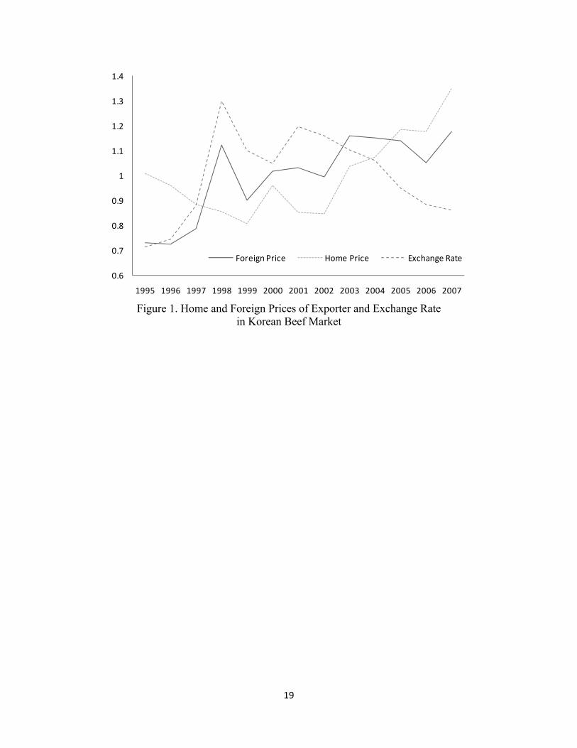
illustrative purposes, it is useful to examine the Korean beef imports market. The foreign prices
of beef imported into the Korean beef market have increased since 2000 with an increase in the
home prices of the exporting countries rather than a decrease in the value of the Korean currency
(Won) against the U.S. dollar.5 In fact, the exchange rate of the Korean Won against the U.S.
dollar decreased during this period of time (see Figure 1). To avoid this problem, previous
studies used the real exchange rate in their empirical econometric models. However, the real
exchange rate is calculated on the basis of a comprehensive price level rather than a specific
commodity’s price level. Furthermore, even if the real commodity exchange rate were calculated
on the basis of the specific commodity price, the effect of a change in the exchange rate on the
foreign price should be separable from the effect of a change in home price. The previous
econometric approach using a gravity trade equation could not provide a theoretical foundation
for this argument.
[Place Figure 1 Approximately Here]
Up to this point, we discussed the endogeneity issue of foreign price depending on the
exchange rate and home price. In order to further develop exchange rate impacts on trade, the
issue of substitutability between home and foreign products in the foreign country must be
discussed. Typically, import demand is determined as the difference between the quantity

7
demanded by foreign consumers and the quantity supplied by foreign producers. Given the home
price of the importing country, a change in the exchange rate directly induces a change in the
foreign price of the exporting country as shown in Equation (1). A change in the foreign price of
the exporting country is likely to induce substitution between home and foreign products. This
substitution affects the home price of the importing country, which is the indirect effect of a
change in exchange rate on the home price of importing country in this study. A change in the
home price of the importing country affects the profit of importing country producers. Therefore,
the effect of a change in the exchange rate on trade flows should be examined in the system of
demand and supply of the importing country.
As a first step to follow this systematic approach, this study uses a constant-elasticity-of-
substitution (CES) utility function of the Dixit-Stiglitz type to examine how a change in the
exchange rate affects on the demand structure of the foreign consumer. From this theoretical
review, the relationship between the exchange rate and both home and foreign prices are
identified. In the CES utility function, the importing country j’s consumer problem in choosing
product, ijQ which is produced in country i and sold in country j or jjQ which is produced and
sold in country j, would be summarized as follows:
(5) ( )[ ]rrjj
rijjj QQAu
1
1 αα −+= , s.t. jjjjjijij mQpQp =+ ,
where jA is a measure of the demand level of country j, α is a share parameter, ω
ω 1−=r
where ω is the elasticity of substitution, and jm is the expenditure of country j on the products.
From (5), we can derive demand equations for jjQ and ijQ of country j as follow:
8
(6.1) ( ) ( )
( ) ( ) ( ) ( ) 111
111
11
11
1 −−−−
−−
+−=
rr
jjrrr
ijr
jrjjr
jj
pp
mpQ
αα
α
,
(6.2) ( ) ( )
( ) ( ) ( ) ( ) 111
111
11
11
1
1
−−−−
−−
+−
−=
rr
jjrrr
ijr
jrijr
ij
pp
mpQ
αα
α
.
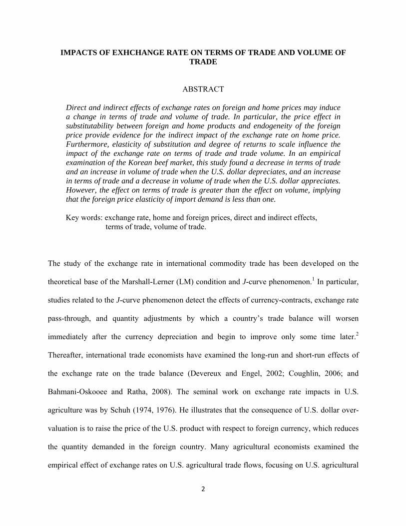
As the above domestic and imports demand equations show, the effect of a change in the
exchange rate on domestic and import demand would be realized through the endogeneity of the
foreign price of the exporting country i. It should be noted that the domestic and import demand
of importing country j would not be affected by the home price when the exchange rate changes,
because there is no direct effect of a change in the exchange rate on the home price of importing
country j when the exchange rate changes. However, it should be noted that the domestic and
import demand equations show a relationship between ije and jjp through a price competition
between ijQ and jjQ and endogeneity of the foreign price of the exporting country.
For the second step, we develop the indirect effect of a change in the exchange rate on the
home price of the importing country. To do this, it is necessary to define the profit maximizing
condition for the producer of importing country j regardless of exchange rate changes. In a
perfectly competitive market, the price is determined through the interaction of both demand and
supply. Each producer would be a price taker and his/her production strategy would be to
maximize his/her profit. Given the home price, how much the foreign producer produces will
depend upon the degree of returns to scale of his/her production technology. This relationship
can be summarized as follows:
(7.1) βπ jjjjjjj kQQp −= ,
(7.2) 1−= ββ jjjj Qkp
9
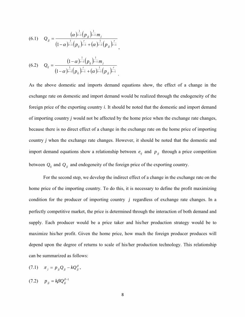
where βkQ is total production cost, 1−ββ jjQk is marginal cost of producing one unit of jjQ , and
β represents the degree of returns to scale of his/her production technology.
The price equation can be used to identify the indirect effect of a change in the exchange
rate on the home price of importing country j, jjp . Because jjQ is defined in equation (6.1), the
home price of importing country j can be expressed with respect to the exchange rate as follows:
(8)
( ) ( )
( ) ( ) ( )ββ
β
ββ
ααβ
αα
)1(
111
11
)1(
111
1
11
11
−
−−−
−
−−−
⎥⎥⎥
⎦
⎤
⎢⎢⎢
⎣
⎡
⎟⎟⎟
⎠
⎞
⎜⎜⎜
⎝
⎛+Φ⎟
⎠⎞
⎜⎝⎛ −
+
⎥⎥
⎦
⎤
⎢⎢
⎣
⎡+Φ⎟
⎠⎞
⎜⎝⎛ −
=
rr
ijrrr
jij
rr
ijrrr
jj
eVmk
e
p
where 0
0
jj
ii
pp
=Φ is the initial ratio of the home prices of country i and j and jiV is the value of
trade from country j to country i.
Furthermore, if country j is a pure importing country, Equation (8) can be simplified. For
example, as Equation (8) shows, if country j is a pure importing country for Q , then jiV will be
zero. As a result, Equation (8) will be reduced as follows:
(9)
( ) ( )
( ) ( ) ββ
β
ββ
β
αα
)1(1
)1(
111
1
11
−
−
−−−
⎥⎥
⎦
⎤
⎢⎢
⎣
⎡+Φ⎟
⎠⎞
⎜⎝⎛ −
=j
rr
ijrrr
jj
mk
e
p
Therefore, the indirect effect of a change in the exchange rate on the home price of importing
country j can be obtained as follows:

10
(10) ( ) ( )
( ) ( )( ) ( )
ββ
ββ
βαα
β
αα
ββ )21(
111
1
)1(1
11
11
1
111
11( −
−−−
−
−−−
⎥⎥
⎦
⎤
⎢⎢
⎣
⎡+Φ⎟
⎠⎞
⎜⎝⎛ −
Φ⎟⎠⎞
⎜⎝⎛ −⎟⎠⎞
⎜⎝⎛
−⎟⎟⎠
⎞⎜⎜⎝
⎛ −
=∂
∂rr
ijrrr
j
rijrrr
ij
jj emk
er
r
ep
.
As equation (10) shows, the direction of the indirect effect of a change in exchange rate
on the home price of importing country j is determined by the degree of returns to scale and
elasticity of substitution of importing country j. This study summarizes the indirect effects of a
change in exchange rate on the home price of importing country j and the direct effects of a
change in exchange rate on the foreign price of exporting country i in Table 1. The direction of
the indirect effects of a change in the exchange rate on the home price of importing country j is
the same as the direction of the direct effects of a change in the exchange rate on the foreign
price of exporting country i when importing country j shows a decreasing returns to scale for the
production technology, given an elastic elasticity of substitution for importing country j.
Therefore, it can be inferred that the terms of trade do not change if the foreign price elasticity
for import demand equals the home price elasticity for import demand and the indirect effect of a
change in exchange rate equals the direct effect of a change in the exchange rate. The direction,
however, differ when importing country j shows an increasing returns to scale of their production
technology given an elastic elasticity of substitution for the importing country j. As a result, the
terms of trade will change due to a change in the exchange rate even when the foreign price
elasticity equals the home price elasticity and the indirect effect equals the direct effect. Given an
inelastic elasticity of substitution of importing country j, the opposite result holds. Table 1 also
shows the relationship between the exchange rate and terms of trade. Regardless the elasticity of
substitution of importing country j and no matter the degree of returns to scale of importing
country j, an appreciate in the exchange rate results in an increase in the terms of trade while a

11
decrease in exchange rate results in a decrease in terms of trade. Since the terms of trade
represents the foreign price relative to the home price, an increase in terms of trade will
deteriorate import demand for foreign products while a decrease in terms of trade will encourage
import demand for foreign products.
[Place Table 1 Approximately Here]
The effect of a change in the exchange rate on trade volume will now be examined using
Equations (1), (6.2), and (9). We obtain the new import demand equation by replacing ijp and
jjp in Equation (6.2) with Equation (1) and (9). The effect of the exchange rate change on
volume of trade shown through the following equation:
(10)
( ) ( ) ( ) ( ) ( )
( ) ( ) ( ) ( ) ( )
( ) ( ) ( )
( ) ( ) ( ) ( ) ( )
( ) ( ) ( ) ( ) ( )
( ) ( ) ( )
( ) ( ) ( ) ( ) ( )
( ) ( ) ( )
2
)1()1(
111
1
11
)1()1(1
11
111
)1(2
111
1
11
)1()1(1
11
11
11
)1(1
11
11
11
)1()1(
111
1
11
)1()1(1
11
111
)1(1
11
12
11
11
1
11)1(
1(
11
1
11
1
11
1
⎥⎥⎥⎥⎥⎥
⎦
⎤
⎢⎢⎢⎢⎢⎢
⎣
⎡
⎥⎥
⎦
⎤
⎢⎢
⎣
⎡+Φ⎟
⎠⎞
⎜⎝⎛ −
+−
⎥⎥⎥⎥⎥⎥⎥⎥⎥⎥⎥⎥⎥⎥⎥⎥⎥⎥⎥⎥⎥
⎦
⎤
⎢⎢⎢⎢⎢⎢⎢⎢⎢⎢⎢⎢⎢⎢⎢⎢⎢⎢⎢⎢⎢
⎣
⎡
⎥⎥⎥⎥⎥⎥⎥⎥⎥
⎦
⎤
⎢⎢⎢⎢⎢⎢⎢⎢⎢
⎣
⎡
⎥⎥⎥⎥⎥⎥
⎦
⎤
⎢⎢⎢⎢⎢⎢
⎣
⎡
⎥⎥
⎦
⎤
⎢⎢
⎣
⎡+Φ⎟
⎠⎞
⎜⎝⎛ −
⎟⎟⎠
⎞⎜⎜⎝
⎛−−
+−⎟⎠⎞
⎜⎝⎛
−
−
−
⎥⎥⎥⎥⎥⎥⎥⎥⎥
⎦
⎤
⎢⎢⎢⎢⎢⎢⎢⎢⎢
⎣
⎡
⎥⎥⎥⎥⎥⎥
⎦
⎤
⎢⎢⎢⎢⎢⎢
⎣
⎡
⎥⎥
⎦
⎤
⎢⎢
⎣
⎡+Φ⎟
⎠⎞
⎜⎝⎛ −
+−
−⎟⎠⎞
⎜⎝⎛
−
=∂
∂
−−
−−−
−
−−
−−−
−−+
−−−
−
−−
−−−
−−
−−−
−−
−−−
−
−−
−−−
−−
−−−
−
rr
rr
ijrrr
r
rr
jriirr
ijr
rrr
rr
ijrrr
r
rr
jriirijr
rr
jriirijr
rr
rr
ijrrr
r
rr
jriirr
ijr
rr
jriirr
ijr
ij
ij
e
mkpe
er
r
mkper
r
mkpe
e
mkpe
mkper
eQ
ββ
ββ
β
βββ
ββ
β
ββ
β
ββ
ββ
β
ββ
β
ααα
βα
αα
ββα
βα
βα
ααα
βα
βα
.

12
As seen in Equation (10), the effect of a change in the exchange rate on trade volume is an
empirical question. However, the effect of a change in the exchange rate on terms of trade and
volume of trade are summarized as follows:
(11) ij
jj
jj
ij
ij
ij
ij
ij
ij
ij
ep
pQ
ep
pQ
eQ
∂
∂
∂
∂+
∂
∂
∂
∂=
∂
∂.
As discussed in Table 1, if a change in the exchange rate does not affect terms of trade given r
and β , then the sign of Equation (11) will be determined by the foreign and home price
elasticities, since the impacts of a change in the exchange rate on both ijp and jjp are same as
each other in the case. Otherwise, it is an empirical question.
Empirical Parameters of the Korean Beef Market
This study has focused on the exchange rate impact on terms of trade and volume of trade in a
microeconomic framework. It seeks to identify the indirect effect of a change in the exchange
rate on the foreign price of an exporting country. For an empirical application of this approach,
this study attempts to estimate the degree of returns to scale for Korean beef production and the
elasticity of substitution for Korean beef consumption using Equations (7.1) and (9), respectively
since these parameters affect the exchange rate. To accomplish these objectives, this study uses
annual data from 1995 to 2007. Home and foreign prices and imported volumes are obtained
from the Korean Customs Service. The United States, Australia, Canada, and New Zealand are
major beef suppliers for Korea. Even though Korea imports from four different countries, U.S.
dollars are used as a medium currency for these transactions. In most cases, exchange rate risk is
borne by Korean beef importers. Korean banks usually provide hedging tools for short-term
exchange rate risk. The exchange rates of the Korean Won and U.S. Dollar are obtained from the
USDA.
13
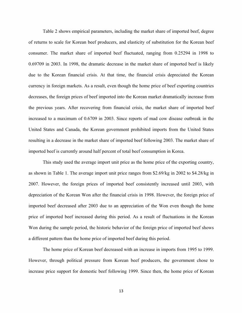
Table 2 shows empirical parameters, including the market share of imported beef, degree
of returns to scale for Korean beef producers, and elasticity of substitution for the Korean beef
consumer. The market share of imported beef fluctuated, ranging from 0.25294 in 1998 to
0.69709 in 2003. In 1998, the dramatic decrease in the market share of imported beef is likely
due to the Korean financial crisis. At that time, the financial crisis depreciated the Korean
currency in foreign markets. As a result, even though the home price of beef exporting countries
decreases, the foreign prices of beef imported into the Korean market dramatically increase from
the previous years. After recovering from financial crisis, the market share of imported beef
increased to a maximum of 0.6709 in 2003. Since reports of mad cow disease outbreak in the
United States and Canada, the Korean government prohibited imports from the United States
resulting in a decrease in the market share of imported beef following 2003. The market share of
imported beef is currently around half percent of total beef consumption in Korea.
This study used the average import unit price as the home price of the exporting country,
as shown in Table 1. The average import unit price ranges from $2.69/kg in 2002 to $4.28/kg in
2007. However, the foreign prices of imported beef consistently increased until 2003, with
depreciation of the Korean Won after the financial crisis in 1998. However, the foreign price of
imported beef decreased after 2003 due to an appreciation of the Won even though the home
price of imported beef increased during this period. As a result of fluctuations in the Korean
Won during the sample period, the historic behavior of the foreign price of imported beef shows
a different pattern than the home price of imported beef during this period.
The home price of Korean beef decreased with an increase in imports from 1995 to 1999.
However, through political pressure from Korean beef producers, the government chose to
increase price support for domestic beef following 1999. Since then, the home price of Korean

14
beef has consistently increased until 2007. In general, the cost structure of the Korean beef
producer demonstrates decreasing returns to scale. The estimated returns to scale parameters of
their cost functions are approximately 1.4 during this sample period. As a result, the estimated
parameter implies that there is an economic restriction on increasing beef production without an
improvement in production technology.
The CES utility assumption restricts the elasticity of substitution. The parameter of
elasticity of substitution is expected to range between ∞− and 1 and should not be zero.
However, this restriction was not satisfied in 1996, 1997, and 1999. This break implies that these
three years cannot explain the effect of a change in the exchange rate on terms of trade and
volume of trade in the economic framework developed by this study. To obtain consistent
interpretation of the simulation, this study eliminated these three years in simulation analysis for
both a depreciation and appreciation of the U.S. dollar.
[Place Table 2 Approximately Here]
Simulation
To simulate the effects of a depreciation and appreciation of the U.S. dollar on terms of trade and
trade volume in the Korean beef import market, this study used the average value of r , ω , and
β during this sample period of time. As mentioned before, three years were eliminated in
calculating the average values of r , ω , and β because 1996, 1997, and 1999 violated the
assumption of the CES utility function. The estimated values of r , ω , and β are -3.0711,
0.3821, and 1.4495, respectively. As a result, Korean showed an inelastic elasticity of
substitution and decreasing returns to scale in production technology. Therefore, the Korean beef
market is categorized by 0<r , 10 << ω , and 1>β .

15
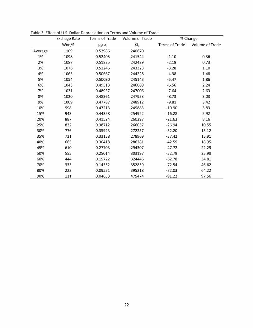
Table 3 and 4 show the results of simulation for a depreciation and appreciation of the
U.S. dollar, respectively. Table 3 shows that a depreciation of the U.S. dollar decreases the terms
of trade. As shown in Table 1, if the indirect effect of a change in the exchange rate on the home
price of Korean beef equals the direct effect of a change in the exchange rate on the foreign price
of imported beef in Korean market, then the terms of trade will be little changed by a
depreciation of the U.S. dollar, given the assumption that the foreign price elasticity for import
demand equals home price elasticity for import demand. Since the empirical results show that the
depreciation of the U.S. dollar decreases the terms of trade, it can be inferred that the direct
effect of a change in exchange rate on the foreign price of imported beef is greater than the
indirect effect of a change in exchange rate on the home price of Korean beef. Furthermore, from
the empirical results, this study infers that the absolute value of the foreign price elasticity for
import demand is less than one because the increase in the trade volume is shown to be less than
the decrease in the terms of trade induced by the depreciation of dollar. The simulation results
show that if the value of the U.S. dollar decreases by 50%, the terms of trade decreases by
52.79% and the volume of trade increases by 25.98%.
Table 4 shows that the appreciation in the value of the U.S. dollar increases the terms of
trade and decreases the volume of trade. These results are consistent with the results of
depreciation. As expected, the impact of the U.S. dollar appreciation on the volume of trade is
much less than the impact of the U.S. dollar appreciation on the terms of trade. However, both an
appreciation and a depreciation of the U.S. dollar show similar effects on the volume of trade and
the terms of trade. If the value of the U.S. dollar increases by 50%, the terms of trade increases
by 56.58% while the trade volume decreases by 14.38%. As a result, the effects of a change in

16
exchange rate on the volume of trade are less than the effects on the terms of trade in both a
depreciation and appreciation of the U.S. dollar.
Conclusion and Further Study
This study identified the effects of a change in the exchange rate on trade flows based on neo-
classical economic principles, since the exchange rate is determined in the foreign exchange
market rather than by agricultural commodity trade. Thus, it is reasonable to believe that the
exchange rate is an exogenous shock on agricultural trade flows. This study identified the direct
effect and indirect effect of a change in the exchange rate on the foreign and home prices
because the foreign price of the exporting country is directly affected by a change in the
exchange rate. At the same time the effects to the home price of importing country may accrue
through the substitutability between home and foreign products and the endogeneity of the
foreign price.
To describe the indirect effect of a change in the exchange rate on the home price of the
importing country, this study used the price equation in which the profit of the importing country
producers is maximized. This study then showed that the marginal effect of the exchange rate on
the home price of the importing country depends on the degree of returns to scale of production
technology and the elasticity of substitution for the importing country. In Table 2, this study
provides the summary of the direct and indirect effects of a change in the exchange rate on the
foreign and home prices and terms of trade along with the degree of returns to scale of
production technology and the elasticity of substitution for the importing country.
To identify the effect of a change in the exchange rate on the volume of trade, this study
derived the marginal import demand equation with respect to the exchange rate. However, this
equation shows that the effect of a change in the exchange rate on the volume of trade is a purely
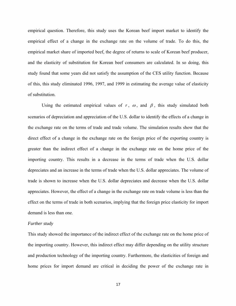
17
empirical question. Therefore, this study uses the Korean beef import market to identify the
empirical effect of a change in the exchange rate on the volume of trade. To do this, the
empirical market share of imported beef, the degree of returns to scale of Korean beef producer,
and the elasticity of substitution for Korean beef consumers are calculated. In so doing, this
study found that some years did not satisfy the assumption of the CES utility function. Because
of this, this study eliminated 1996, 1997, and 1999 in estimating the average value of elasticity
of substitution.
Using the estimated empirical values of r , ω , and β , this study simulated both
scenarios of depreciation and appreciation of the U.S. dollar to identify the effects of a change in
the exchange rate on the terms of trade and trade volume. The simulation results show that the
direct effect of a change in the exchange rate on the foreign price of the exporting country is
greater than the indirect effect of a change in the exchange rate on the home price of the
importing country. This results in a decrease in the terms of trade when the U.S. dollar
depreciates and an increase in the terms of trade when the U.S. dollar appreciates. The volume of
trade is shown to increase when the U.S. dollar depreciates and decrease when the U.S. dollar
appreciates. However, the effect of a change in the exchange rate on trade volume is less than the
effect on the terms of trade in both scenarios, implying that the foreign price elasticity for import
demand is less than one.
Further study
This study showed the importance of the indirect effect of the exchange rate on the home price of
the importing country. However, this indirect effect may differ depending on the utility structure
and production technology of the importing country. Furthermore, the elasticities of foreign and
home prices for import demand are critical in deciding the power of the exchange rate in

18
affecting the terms of trade and trade volume. In the future, it will be important to analyze
consumer and producer behavior in response to a change in home and foreign prices in the
importing country. Furthermore, this framework could be extended to a pure bilateral trade
model in which both countries simultaneously import and export. The indirect effect of the
exchange rate in that scenario will be more complicated. However, through expansion of this
approach, it will add clarity to how the exchange rate impacts import demand.
19
0.6
0.7
0.8
0.9
1
1.1
1.2
1.3
1.4
1995 1996 1997 1998 1999 2000 2001 2002 2003 2004 2005 2006 2007
Foreign Price Home Price Exchange Rate
Figure 1. Home and Foreign Prices of Exporter and Exchange Rate
in Korean Beef Market

20
Table 1. Direct and indirect effects of exchange rate on foreign and home prices.
0 < r < 1 (ω>1) r < 0 (ω <1) β > 1 β = 1 β < 1 β > 1 β = 1 β < 1
ij
ij
ep∂
∂
↑ije (+) (+) (+) (+) (+) (+) ↓ije (-) (-) (-) (-) (-) (-)
ij
jj
ep∂
∂
↑ije (+) (0) (-) (-) (0) (+) ↓ije (-) (0) (+) (+) (0) (-)
jj
ij
pp
↑ije 0 (+) (+) 0 (+) 0 ↓ije 0 (-) (-) 0 (-) 0

21
Table 2. Annual Empirical Parameters of Korean Beef Consumer and ProducerT pii pij pjj Qij Qjj eij α β r ω
1995 3.19 2463 5288 168367 154700 771.27 0.52115 1.44479 ‐9.02743 0.09971996 3.04 2444 5147 163360 174000 804.45 0.48423 1.44782 11.80448 ‐0.09261997 2.80 2660 5143 166091 237000 951.29 0.41204 1.44123 1.85493 ‐1.16971998 2.71 3793 4345 92026 271800 1401.44 0.25294 1.42799 0.125358 1.14331999 2.55 3037 4147 177479 239700 1188.82 0.42543 1.42050 1.036198 ‐27.62622000 3.04 3436 4587 237943 214100 1130.96 0.52637 1.42329 ‐2.7347537 0.26782001 2.70 3483 5408 180631 164400 1290.99 0.52352 1.43821 ‐4.6745045 0.17622002 2.69 3359 6545 315887 147400 1251.09 0.68184 1.44810 ‐0.8750452 0.53332003 3.29 3918 6512 325865 141600 1191.61 0.69709 1.45795 ‐0.6096377 0.62132004 3.40 3893 6112 160126 144900 1145.32 0.52496 1.46249 ‐4.51405 0.18142005 3.76 3848 6460 178331 152400 1024.12 0.53920 1.46268 ‐3.297409 0.23272006 3.72 3556 7085 212782 158200 954.79 0.57356 1.46113 ‐2.3256988 0.30072007 4.28 3975 7938 219607 171200 929.26 0.56193 1.46822 ‐2.7777047 0.2647Mean 3.17 3374 5747 199884 182415 1079.65 0.51725 1.44649 ‐1.23194 ‐1.92826α: market share of imported beefpii: home price of exporting country's beef ($/kg)
pij: foreign price of exporting country's beef (Korean Won/kg)
pjj: home price of Korean beef (Won/kg)
Qij: imported beef (1000kg)
Qjj: Korean beef (1000kg)β: degree of returns to scale of productioneij: Korean Won and U.S. dollar exchange rate (Korean Won/U.S.$)r: parameter of elasticity of substitutionω: elasticity of substitution
22
Table 3. Effect of U.S. Dollar Depreciation on Terms and Volume of TradeExchage Rate Terms of Trade Volume of Trade
Won/$ pij/pjj Qij Terms of Trade Volume of Trade
Average 1109 0.52986 2406701% 1098 0.52405 241544 ‐1.10 0.362% 1087 0.51825 242429 ‐2.19 0.733% 1076 0.51246 243323 ‐3.28 1.104% 1065 0.50667 244228 ‐4.38 1.485% 1054 0.50090 245143 ‐5.47 1.866% 1043 0.49513 246069 ‐6.56 2.247% 1031 0.48937 247006 ‐7.64 2.638% 1020 0.48361 247953 ‐8.73 3.039% 1009 0.47787 248912 ‐9.81 3.4210% 998 0.47213 249883 ‐10.90 3.8315% 943 0.44358 254922 ‐16.28 5.9220% 887 0.41524 260297 ‐21.63 8.1625% 832 0.38712 266057 ‐26.94 10.5530% 776 0.35923 272257 ‐32.20 13.1235% 721 0.33158 278969 ‐37.42 15.9140% 665 0.30418 286281 ‐42.59 18.9545% 610 0.27703 294307 ‐47.72 22.2950% 555 0.25014 303197 ‐52.79 25.9860% 444 0.19722 324446 ‐62.78 34.8170% 333 0.14552 352859 ‐72.54 46.6280% 222 0.09521 395218 ‐82.03 64.2290% 111 0.04653 475474 ‐91.22 97.56
% Change

23
Table 4. Effect of U.S. Dollar Appreciation on Terms and Volume of TradeExchage Rate Terms of Trade Volume of Trade
Won/$ pij/pjj Qij Terms of Trade Volume of Trade
Average 1109 0.52986 2406701% 1120 0.53568 239804 1.10 ‐0.362% 1131 0.54151 238948 2.20 ‐0.723% 1142 0.54734 238102 3.30 ‐1.074% 1153 0.55318 237264 4.40 ‐1.425% 1165 0.55903 236435 5.50 ‐1.766% 1176 0.56488 235614 6.61 ‐2.107% 1187 0.57075 234802 7.72 ‐2.448% 1198 0.57662 233998 8.82 ‐2.779% 1209 0.58250 233203 9.93 ‐3.1010% 1220 0.58839 232415 11.04 ‐3.4315% 1275 0.61793 228591 16.62 ‐5.0220% 1331 0.64766 224945 22.23 ‐6.5325% 1386 0.67757 221462 27.88 ‐7.9830% 1442 0.70766 218128 33.55 ‐9.3735% 1497 0.73792 214932 39.27 ‐10.6940% 1553 0.76834 211864 45.01 ‐11.9745% 1608 0.79893 208914 50.78 ‐13.1950% 1664 0.82968 206073 56.58 ‐14.3860% 1775 0.89166 200693 68.28 ‐16.6170% 1885 0.95425 195673 80.09 ‐18.7080% 1996 1.01743 190971 92.02 ‐20.6590% 2107 1.08119 186550 104.05 ‐22.49
% Change

24
Footnote 1. According to Marshall-Lerner condition, in order to improve the trade balance when a currency devalues, the sum of import and export demand elasticities should exceed unity. However, there have been circumstances under which this condition was satisfied yet the trade balance continued to deteriorate. The focus, therefore, has shifted to the short-run dynamics that trace the post-devaluation time-path of the trade balance, i.e., the J-Curve phenomenon (Bahmani-Oskooee, 2004). Footnote 2. See Magee (1973) and Bahmani-Oskooee and Ratha (2004). Footnote 3.
As a result, even though ii
ijij p
pe = is true, 0=
∂
∂
ij
ij
pe
and 0=∂
∂
ii
ij
pe
.
Footnote 4. Given transportation costs and barriers to trade the absolute version of the law of one price rarely holds. Instead, the foreign price equation would be augmented by market distorting parameter, γ as follows: iiijjij pep γ= , where jγ represents supplemental costs when the goods flow from country i to country j.
Footnote 5. Although the U.S. is not the only exporting country, all beef trade is denominated in U.S. dollars. Major exporting countries include the United States, Australia, Canada, and New Zealand. Among them, the United States and Australia are the biggest exporters.

25
Refferences
Bahmani-Oskooee, M., and A. Ratha. “The J-Curve: a literature review.” Applied Economics 36(2004):1377-98.
Carter, C.A., and D.H. Pick. “The J-Curve Effect and the U.S. Agricultural Trade Balance.” American Journal of Agricultural Economics 71(1989):713-20.
Chambers, R.G., and R.E. Just. “Effects of Exchange Rate Changes on U.S. Agriculture: A Dynamic Analysis.” Amer. J. Agr. Econ. 63(1981):32-46.
Cho G., I.M. Sheldon, and S. McCorriston. “Exchange Rate Uncertainty and Agricultural Trade.” Amer. J. Agr. Econ. 84(2002):931-42.
Devereux, M.B., and C. Engel. “Exchange Rate Pass-Through, Exchange Rate Volatility, and Exchange Rate Disconnect.” Journal of Monetary Economics. 49(2002):913-40.
International Monetary Fund. International Financial Statistics, August 2008.
Kandilov, I.T. “The Effects of Exchange Rate Volatility on Agricultural Trade.” Amer. J. Agr. Econ. 90(2008):1028-43.
Konandreas, P., P. Bushnell, and R. Green. “Estimation of Export Demand functions for U.S. Wheat.” West. J. Agr. Econ. 3(1978):39-49.
Korean Customs Services. Statistical Database for Volume and Value of Imports. Internet website: http://portal.customs.go.kr/kcsipt/portal_link_index.jsp?&portalGoToLink=portals_submain_busine_08&iFrameGoToLink=/CmnPt/jsp/JDCQ000.jsp (Accessed August 2007).
Krugman P.R., and M. Obstfeld. “International Economics.” 3rd Edition, p.466-469 (2000).
Magee, S.P. Currency Contracts, Pass Through and Devaluation.” Brooking papers on Economic Activity, 1(1973):303-25.
Pick, D.H., and T.A. Park. “Exchange Rate Risk and U.S. Agricultural Trade Flow.” Amer. J. Agr. Econ. 72(1990):694-700.
Pollard, P.S., and C.C. Coughlin. “Passthrough Estimates and the Choice of an Exchange Rate Index.” Review of International Economics. 14(2006):535-53.
Schuh, E.G. “The Exchange Rate and U.S. Agriculture.” Amer. J. Agr. Econ. 56(1974):1-13.
_____. “The New Macroeconomics of Agriculture.” Amer. J. Agr. Econ. 58(1976):802-11.