Impact of XPM and FWM on the digital implementation of impairment compensation for WDM transmission using backward propagation

Impact of XPM and FWM on the digitalimplementation of impairment

compensation for WDM transmissionusing backward propagation

Eduardo Mateo, Likai Zhu and Guifang LiCREOL: The College of Optics and Photonics, University of Central Florida; 4000 Central

Florida Blvd, Orlando Florida, 32816.

[email protected]

Abstract: The impact of cross-phase modulation (XPM) and four-wavemixing (FWM) on electronic impairment compensation via backward prop-agation is analyzed. XPM and XPM+FWM compensation are comparedby solving, respectively, the backward coupled Nonlinear SchrodingerEquation (NLSE) system and the total-field NLSE. The DSP implemen-tations as well as the computational requirements are evaluated for eachpost-compensation system. A 12×100 Gb/s 16-QAM transmission systemhas been used to evaluate the efficiency of both approaches. The resultsshow that XPM post-compensation removes most of the relevant source ofnonlinear distortion. While DSP implementation of the total-field NLSEcan ultimately lead to more precise compensation, DSP implementationusing the coupled NLSE system can maintain high accuracy with bettercomputation efficiency and low system latency.

© 2008 Optical Society of America

OCIS codes: (060.2330) Fiber optics communications; (060.1660) Coherent communications.(190.4370) Nonlinear optics, fibers.

References and links1. D. Marcuse, A. R. Chraplyvy and R. W. Tkach, “Effect of fiber nonlinearity on long-distance transmission,” J.

Lightwave Technol. 9, 121–129 (1991).2. S. Watanabe and M. Shirasaki, “Exact compensation for both chromatic dispersion and Kerr effect in a transmis-

sion fiber using optical phase conjugation,” J. Lightwave Technol. 14, 243–249 (1996).3. C. Kurtzke, “Suppression of fiber nonlinearities by appropriate dispersion management,” J. Lightwave Technol.

5, 1250–1253 (1993).4. J. Leibrich, C. Wree and W. Rosenkranz, “CF-RZ-DPSK for suppression of XPM on dispersion-managed long-

haul optical WDM transmission on standard single-mode fiber,” IEEE Photon. Technol. Lett. 14, 155–157 (2002).5. S. L. Woodward, S. Huang, M.D. Feuer, and M. Boroditsky, “Demonstration of an electronic dispersion com-

pensation in a 100-km 10-Gb/s ring network,” IEEE Photon. Technol. Lett. 15, 867–869 (2003).6. K. Roberts, C. Li, L. Strawczynski, M. OSullivan, and I. Hardcatle, “Electronic precompensation of optical

nonlinearity,” IEEE Photon. Technol. Lett. 18, 403–405 (2006).7. E. Yamazaki, F. Inuzuka, K. Yonenaga, A. Takada, and M. Koga, “Compensation of interchannel crosstalk in-

duced by optical fiber nonlinearity in carrier phase-locked WDM system,” IEEE Photon. Technol. Lett. 19, 9–11(2007).

8. X. Li, X. Chen, G. Goldfarb, E. Mateo, I. Kim, F. Yaman and G. Li, “Electronic post-compensation of WDMtransmission impairments using coherent detection and digital signal processing,” Opt. Express 16, 880–889(2008).

9. G. P. Agrawal, Nonlinear fiber optics, (Academic Press, 2007).

(C) 2008 OSA 29 September 2008 / Vol. 16, No. 20 / OPTICS EXPRESS 16124#96880 - $15.00 USD Received 30 May 2008; revised 24 Jun 2008; accepted 25 Jun 2008; published 26 Sep 2008

10. J. Leibrich and W. Rosenkranz, “Efficient numerical simulation of multichannel WDM transmission systemslimited by XPM,” IEEE Photon. Technol. Lett. 15, 395–397 (2003).

11. O. V. Sinkin, Holzlohner, J. Zweck and C. Menyuk,” “Optimization of the split-step Fourier method in modellingoptical-fiber communications system,” J. Lightwave Technol. 21, 61–68 (2003).

12. T. Schneider, Nonlinear optics in telecommunications, (Springer, 2004).13. G. Bosco, A. Carena, V. Curri, R. Gaudino, P. Poggiolini and S. Benedetto, “Suppression of spurious tones

induced by the split-step method in fiber systems simulation,” IEEE Photon. Technol. Lett. 12, 489–397 (2000).14. G. Goldfarb, G. Li and M. G. Taylor, “Orthogonal wavelength-division multiplexing using coherent detection,”

IEEE Photon. Technol. Lett. 19, 2015–2017 (2007).15. X. Liu and D. A. Fishman, “A fast and reliable algorithm for electronic pre-equalization of SPM and chromatic

dispersion,” in OFC 1996 , paper OThD4.16. A. J. Lowery, L. B. Du and J. Armstrong, “Performance of optical OFDM in ultralong-haul WDM lightwave

systems,” J. Lightwave Technol. 25, 131–138 (2007).17. M. Shtaif, M. Eiselt and L. D. Garret, “Cross-phase modulation distortion measurements in multispan WDM

systems,” IEEE Photon. Technol. Lett. 12, 88–90 (2000).18. P. P. Mitra and J. B. Stark, “Nonlinear limits to the information capacity of optical fibre communications,” Nature

411, 1027–1030 (2001).19. J. M. Kahn and K. Ho, “Spectral efficiency limits and modulation/detection techniques for DWDM systems,”

IEEE J. Sel. Top. Quantum Electron. 10, 259–272 (2004).20. J. Wang and K. Petermann, “Small signal analysis for dispersive optical fiber communication systems,” J. Light-

wave Technol. 10, 96–100 (1992).21. T. Yu, W. M. Reimer, V. S. Grigoryan and C. R. Menyuk, “A mean field approach for simulating wavelength-

division multiplexed systems,” IEEE Photon. Technol. Lett. 12, 443–445 (2000).

1. Introduction

In long-haul fiber transmission systems, fiber chromatic dispersion (CD), Kerr nonlinearityand amplifier noise are responsible for signal degradation, limiting the capacity of wavelength-division multiplexed (WDM) transmission systems [1]. Over the past few years, optical tech-niques such as dispersion management or mid-span phase conjugation [2], have been exten-sively studied and deployed to mitigate the degrading effects in fibers [3, 4]. Recently, electronicpre- and/or post-compensation of transmission impairments have attracted significant attentiondue to the fast development of coherent detection and digital signal processing (DSP), whichconstitute the enabling technologies for electronic impairment compensation [5, 6, 7].

In particular, post-compensation schemes offer a great flexibility since adaptive compensa-tion can be incorporated, improving the robustness against modifications on the physical layer.In the context of WDM transmission, our group recently proposed a universal post-processingscheme [8] where, for the first time to our knowledge, dispersive and nonlinear intra- and inter-channel impairments are fully compensated using electronic backward propagation. In [8], thetotal optical DWM signal is backward propagated using a full time-domain split-step methodto solve the z-reversed nonlinear Schrodinger equation (NLSE). Although this method has beenproven effective, reducing the number of computations required and its impact on the systemlatency is desirable for the eventual implementation of the post-compensation method.

In this paper, the impact of nonlinear inter-channel effects, i.e. cross-phase modulation(XPM) and four-wave mixing (FWM), are studied in the framework of backward propaga-tion post-compensation systems. For this purpose, a WDM transmission system with 12 chan-nels, each of them modulated in a 100 Gbits/s 16-QAM format, is simulated. This modulationformat is selected because it provides high spectral efficiency and nonlinear impairment com-pensation becomes necessary for long-distance transmission. The impact of XPM and FWMon post-compensation using backward propagation will be evaluated individually, by solvingrespectively, the coupled NLSE system (C-NLSE) and the total-field NLSE (T-NLSE) using thesplit-step Fourier method (SSFM). The impact of both effects on the detected Q-factor, opti-mum launching power and channel spacing will be analyzed in detail. Additionally, generalizedconclusions about the DSP computational requirements for each compensation scheme will be


presented for WDM systems.This paper is structured as follows. In section 2, the governing equations for XPM and

XPM+FWM compensation will be introduced, focusing on the numerical aspects involved onthe SSFM for each case. In section 3, the results of this work will be presented followed by thediscussion and conclusion.

2. Theory of backward propagation compensation and digital implementation

2.1. Backward propagation equations and numerical procedure

In a coherent detection system, a full reconstruction of the optical field can be achieved by beat-ing the received field with a co-polarized local oscillator. The reconstructed field will be used asthe input for backward propagation in order to compensate the transmission impairments. LetEm be the envelope of the mth-channel field where m ∈ I, I = {1,2, · · · ,N} and N is the totalnumber of WDM channels. By rewriting the field expression as, Em = Em exp(imΔωt), whereΔ f = Δω/2π is the channel spacing, the expression of the full optical field can be expressedas, E = ∑m Em. The total-field back propagation equation, i.e T-NLSE, is given by [9],

−∂E∂ z

+α2

E +iβ2

2∂ 2E∂ t2 − β3

6∂ 3E∂ t3 − iγ|E|2E = 0, (1)

where β j represent the jth-order dispersion, α is the absorption coefficient, γ is the nonlinearparameter and t is the retarded time [9]. Equation (1) governs the backward propagation of thetotal field including second and third order dispersion, SPM, XPM and FWM compensation.

Alternatively, the effect of FWM can be omitted in backward propagation by introducing theexpression for E into Eq. (1), expanding the |E| 2 term and neglecting the so-called FWM terms,that is,

−∂Em

∂ z+

α2

Em +iβ2

2∂ 2Em

∂ t2 − β3

6∂ 3Em

∂ t3 − iγ

(2 ∑

q∈I|Eq|2 −|Em|2

)Em = 0. (2)

The system of coupled equations (2) describe the backward evolution of the WDM channelswhere dispersion, SPM and XPM are compensated.

The above equations are solved by means of the split-step Fourier method (SSFM) [10, 11].Here, the dispersive and nonlinear contributions are considered to be independent in a shortsegment of propagation. The length of this segment, i.e. step size, is determined according tothe characteristics of the system under study and it should be selected carefully in order topreserve the accuracy of the results. In this work, we will use the symmetric step size where thenonlinear part is estimated by averaging the optical power over the the step length in a iterativeway (the details of this procedure can be found in [8, 9]). Although this method increases thenumber of computations per step, it allows to increase the step size in such a way that thetotal number of operations is reduced without accuracy penalty. In Fig. 1 it is depicted a blockdiagram of the SSFM for a single step and for Eq. (1), where two iterations (sub-steps) for thepower averaging are performed.

The involved operators in the SSFM are given by, D(x) = F −1 [HF (x)], P(x) = |x|2 andE(x) = exp(iγxh), where the transfer function H for fiber dispersion and loss is given by,

H(ω) = exp

[(α2

+ iβ2ω2

2+ iβ3

ω3

6

)h2

],

with ω being the angular frequency and h the step size.Likewise, Eqs. (2) are also solved by the SSFM, following the procedure depicted in Fig. 2,

again, for a single step. In contrast to the total-field NLSE, a sum operation is included at each


Fig. 1. Block diagram of the DSP implementation of the total-field NLSE.

Fig. 2. Block diagram of the DSP implementation of coupled NLSEs.

sub-step to include the XPM contribution on each channel. Finally, for a given optical link withM spans, the iterative procedure for SSFM backward propagation is given by the block diagramshown in Fig. 3 where ns is the number of steps per span (note that an attenuation element hasbeen introduced to compensate the amplification stages).

Fig. 3. SSFM backward propagation diagram for a M-spans optical link.

2.2. SSFM Step size and digital implementation efficiency

As it was mentioned before, the number of operations required for SSFM backward propagationis of great importance in digital post-processing. The number of operations for a given spandepends on the number of steps (ns), and hence, on the step size (h = L/ns) where L is thespan length. The SSFM accuracy depends fundamentally on the mutual influence of dispersionand nonlinearity within the step length. Due to the nature of the dispersion and nonlinearityoperators, the step size has to make sure that: (1) the nonlinear phase shift is small enough topreserve the accuracy of the dispersion operation and (2) the optical power fluctuations due to


dispersion effects are small enough to preserve the accuracy of the nonlinear operation.One way to set the upper bound for the step size is to identify the characteristic physical

lengths of the transmission system, which correlate the optical field fluctuations with the prop-agation distance. Three physical lengths are of interest here, namely, the nonlinear length L nl,the walk-off length Lwo and the four-wave mixing length L fwm. The nonlinear and walk-offlengths can be defined, for a multi-channel system, as follows,

Lnl =1

γPT2N −1

N

, Lwo =1

2π |β2|(N −1)Δ f B, (3)

where, PT = ∑m |Em|2 is the total launched power and B is the symbol rate (effectively theinverse of the pulse width). The nonlinear length has been defined as the length after whichan individual channel experiences a 1 radian phase shift due to SPM and XPM. The walk-offlength is defined as the distance after which the relative delay of pulses from the edge channelsis equal to the pulse width. The above characteristic lengths are well known [12] and widelyused to qualitatively describe the optical field behavior through fiber propagation However,when FWM is considered, the nonlinear and walk-off lengths are not enough to qualitativelyidentify the range where the fastest field fluctuations take place. In order to identify the fastestfield fluctuations due to FWM, the total optical field should be rewritten as E = ∑m Em exp(ikmz)where km is the linear propagation constant of the mth-channel. By following the same proce-dure as for Eq. (2), the nonlinear term, now including FWM, can be expressed as follows forthe mth-channel,

−iγ

(2 ∑

q∈I

|Eq|2 −|Em|2)

Em − iγ

[∑

[rslm]∈I

ErEsE∗l exp(iδkrslmz)

], (4)

whith the following conditions l = r + s−m, [m,r,s] ∈ I and r �= s �= m. The first conditionneglects fast time-oscillating terms (frequency matching). The second condition forces the newgenerated waves to lay within the WDM band. Finally, the third condition excludes SPM andXPM terms. δkrslm is the phase mismatch parameter, given by,

δkrslm = kr + ks − kl − km =12

β2Δω2[r2 + s2 − (r + s−m)2−m2]. (5)

In order to identify the fastest z-fluctuations for the mth-channel, let us set r = 1 and s = Ncorresponding to the indexes of the edge channels. By maximizing Eq. (5), the expression forthe maximum phase-mismatch is given by,

δkmax =14|β2|(N −1)2Δω2. (6)

The above expression leads to the following definition for the FWM length,

Lfwm =1

π2|β2|(N −1)2Δ f 2 . (7)

The above expression represents the length after which the argument of the fastest FWMterm is shifted by 1 radian; hence, it can be understood as the distance after which powerfluctuations due to FWM start to take place. The definition of the FWM length assumes thatthe FWM-induced variations on a given channel are governed by the linear (dispersive) phasemismatch. However, nonlinearity also contribute to the overall phase mismatch through SPM


and XPM. This contribution is only relevant in high power regimes and it is not expected toplay a role in the analysis of fiber transmission. The SSFM step size will be correlated to theminimum characteristic length involved in each case; thus, for the compensation of SPM andXPM effects via coupled equations, the step size is limited by the walk-off length whereas theFWM length will be the parameter limiting the step size for the total-field NLSE. For WDMsystems , the nonlinear length is longer than the FWM and walk-off lenghts for the typicallaunch powers of interest in communications.

Although variable step-size schemes have been used to reduce the number of operationsrequired to describe FWM in fibers [13], a constant step size will be considered is this paper.The variable step size technique corrects the spurious FWM tones generated by a wrong stepsize distribution. However, the computational efficiency of this technique rapidly decreases inmulti-channel and/or large dispersion systems [11], where the generation of spurious tones isnot the only source of error. In addition, it is important to note that a constant step size presentsa great practical advantage in the eventual realization of the DSP post-processor.

The following relationships define the characteristic step sizes for XPM and FWM compen-sation via the iterative symmetric SSFM, i.e,

hwo = τrLwo, hfwm = φfwmLfwm, (8)

where the dimensionless parameters τr and φfwm represent, respectively, the maximum inter-pulse relative delay (with respect to the pulse width) and the maximum phase-mismatch allowedwithin one step.

The values of τr and φfwm may depend on several factors including the impact of non-deterministic fluctuations on the system (ASE and laser phase noise), the desired degree ofaccuracy and most importantly, the numerical procedure (in our case the iterative symmet-ric SSFM). Thus, those parameters are usually determined a posteriori within the simulationresults. However, it is important to stress that, although τr and φfwm can be understood as phe-nomenological parameters, their values are related to the numerical procedure itself and theyare expected to be independent on the general WDM transmission parameters, such as channelspacing or number of channels, whose effect over the step size is governed by the physicallengths. In addition, provided that the SSFM is used for both the T-NLSE and the C-NLSE, theratio κ = τr/φfwm can be regarded as a constant for any variant of the split-step Fourier method.

In order to gain a perspective on the computational requirements for each method, it is inter-esting to evaluate the number of operations required for FWM and/or XPM compensation. Forsimplicity, the number of operations in the XPM modules shown in Fig. 2 is neglected. This isjustified because, in general, dispersion modules require a large computational load. Since thetotal number of computations is inversely proportional to the step size,

Cfwm

Cxpm=

hxpm

Nhfwm=

πκ2

(N −1)Δ fNB

, (9)

where C represents total number of operations. Note that the the XPM characteristic step sizedictates the number of operations per channel; thus, the total number of operations for XPMcompensation is multiplied in Eq. (9) by the total number of channels.

It is interesting to note that this ratio becomes asymptotically independent of the number ofchannels for N � 1. This is an expected result since the scaling of Lwo and Lfwm with N iscompensated by the number of coupled equations that have to be solved for XPM compensa-tion. On the other hand, the number of computations for FWM compensation grows with theratio between the channel spacing and the symbol-rate. This means that the cost for FWM com-pensation decreases in systems with a high spectral efficiency, where the channels are highlyphase-matched and larger step sizes can be used to describe the field propagation. It is also


interesting to note that the above ratio is independent of the fiber chromatic dispersion. This in-dicates that the above ratio can be generalized to dispersion-managed systems provided that thedominant characteristic lengths are related to dispersive effects, as expected in WDM systems.

Together with number of computations, the latency of the post-processor is of great relevancein communications, especially for real-time applications. A fundamental difference arises be-tween the impairment compensation via coupled or total-field equations. As shown in Fig.2, the coupled equations for XPM compensation naturally parallelize post-processing, whichdrastically reduces the latency of the system. For FWM compensation via T-NLSE, the sys-tem latency is proportional to the number of operations per step (τ fwm ∝ Cfwm). However, forXPM compensation via C-NLSE, the system latency (τxpm) is proportional to the number ofoperations per step and per channel; hence, the following relationship can be obtained for theprocessing latency,

τfwm

τxpm=

hxpm

hfwm=

πκ2

(N −1)Δ fB

. (10)

Again, the XPM module is omitted in the analysis. This module is expected to add a smallcorrection to the processing latency for XPM compensation. Note that the above expression isindependent of any additional parallelization, which can be done to the C-NLSE and T-NLSEsystems without distinction. Eq. (10) indicates that FWM compensation leads to a latency thatgrows with the total WDM optical bandwidth.

The results obtained so far, show the great importance of individually identify the impactof XPM and FWM on the WDM transmission in order to be able to select the most efficientpost-processing scheme.

3. Simulation results

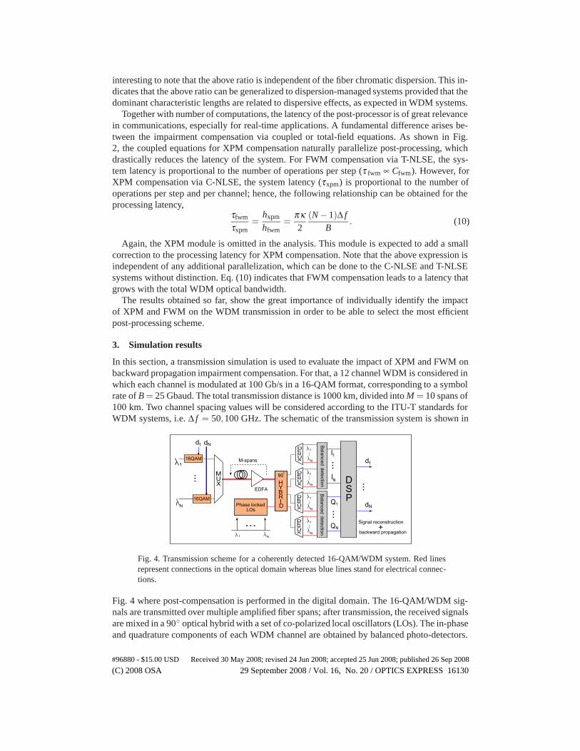
In this section, a transmission simulation is used to evaluate the impact of XPM and FWM onbackward propagation impairment compensation. For that, a 12 channel WDM is considered inwhich each channel is modulated at 100 Gb/s in a 16-QAM format, corresponding to a symbolrate of B = 25 Gbaud. The total transmission distance is 1000 km, divided into M = 10 spans of100 km. Two channel spacing values will be considered according to the ITU-T standards forWDM systems, i.e. Δ f = 50,100 GHz. The schematic of the transmission system is shown in

Fig. 4. Transmission scheme for a coherently detected 16-QAM/WDM system. Red linesrepresent connections in the optical domain whereas blue lines stand for electrical connec-tions.

Fig. 4 where post-compensation is performed in the digital domain. The 16-QAM/WDM sig-nals are transmitted over multiple amplified fiber spans; after transmission, the received signalsare mixed in a 90◦ optical hybrid with a set of co-polarized local oscillators (LOs). The in-phaseand quadrature components of each WDM channel are obtained by balanced photo-detectors.


Analog-to-digital (A/D) conversion is followed by DSP field reconstruction, backward propa-gation, demultiplexing and data recovery. Using coherent detection, each channel is translatedto baseband and sampled at 25 Gsa/s (i.e. 1 sample per symbol). Then, 32/64 samples areadded to each symbol (respectively for Δ f = 50/100 GHz) and the 12 channels are combinedto reconstruct a final optical waveform of 800/1600 GHz bandwidth (corresponding to an up-sampled transmitted bandwidth of 600/1200 GHz). The details of the DSP implementation ofthe up-sampling procedure can be found in [8].

The transmission channel is a non-zero dispersion shifted fiber, with: β 2 = −5.63 ps2/km(D = 16 ps/km/nm), β3 = 0.083 ps3/km, α = 0.046 km−1 (0.2 dB/km) and γ = 1.46 W−1km−1.The signal is amplified after each span with an EDFA with a noise figure of 5 dB. For simplicity,the laser phase noise is neglected.

Clearly, backward propagation requires an accurate knowledge of the link parameters. Fromthe practical point of view, training experiments can be done to set the link parameters whichoptimize the performance. In addition, small fluctuations on the optical link due to environmen-tal effects are expected to have a small impact on the performance [15].

Forward transmission simulations have been made using VPItransmissionMaker where twodifferent channel spacings and nine different input power values had been considered. Back-ward propagation algorithms are developed in Matlab where C-NLSE and T-NLSE are solvedwith different step sizes for each case. As a preliminary illustration, in Fig. 3 are shown theconstellation and eye diagrams as well as the Q-factor values for, respectively, back-to-back,dispersion compensation only and XPM compensation via C-NLSE. The results are given forone of the central channels (which presents the highest inter-channel nonlinear distortion). TheQ-factor is obtained from the constellation diagram as in [16].

−1.5 −1 −0.5 0 0.5 1 1.5−1.5

−1

−0.5

0

0.5

1

1.5(A)

−1.5 −1 −0.5 0 0.5 1 1.5−1.5

−1

−0.5

0

0.5

1

1.5(B)

−1.5 −1 −0.5 0 0.5 1 1.5−1.5

−1

−0.5

0

0.5

1

1.5(C)

0 10 20 30 40 50 60 70−2

−1.5

−1

−0.5

0

0.5

1

1.5

2

time (ps)

(A)

0 10 20 30 40 50 60 70−2

−1.5

−1

−0.5

0

0.5

1

1.5

2

time (ps)

(B)

0 10 20 30 40 50 60 70−2

−1.5

−1

−0.5

0

0.5

1

1.5

2

time (ps)

(C)

Fig. 5. Constellation and eye diagrams for one of the central channels (PT = 9 dBm). (A)Back-to-back (Q = 29.8 dB); (B) Dispersion compensation (Q = 8.3 dB) and (C) XPMcompensation with 30 steps per span (Q = 13.3 dB).

The compensation of XPM clearly gives rise to a well defined constellation and better eyeopening, as shown in Fig. 3-(C), in comparison with no nonlinearity compensation as shown inFig. (3)-(B). It should be noted, though, that the number of operations for only dispersion com-pensation is drastically reduced, corresponding to a single-step linear operation on the SSFM.Next, an exhaustive analysis of the two compensation schemes is made, starting with a channelspacing of 50 GHz.


A. Results for Δ f = 50 GHz

Fig. 6 shows the Q-factor values as a function of to the total input power for different step sizes.

6 7 8 9 10 11 12 13 145

6

7

8

9

10

11

12

13

14

15

Total Power (dBm)

Q (

dB)

(A)

h=10 kmh= 6.7 kmh=5 kmh=3 km

6 7 8 9 10 11 12 13 146

7

8

9

10

11

12

13

14

15

16

Total Power (dBm)

Q (

dB)

(B)

h=1 kmh=500 mh=333 mh=181 m

Fig. 6. Received Q-factor for Δ f = 50 GHz with: (A) XPM compensation via C-NLSE and(B) FWM compensation via T-NLSE.

The results show the well-known optimum power for optical transmission in nonlinear sys-tems, where the post-compensation of deterministic effects provide the maximum Q-factor.Above the optimum power, the non-deterministic nonlinear distortion due to signal-ASE beatstarts to offset the SNR growth with launching power.

The characteristic step sizes for the 50 GHz channel spacing take the values of h wo = 3.08km and hfwm = 178 m, with τr = 3/2 and φ f wm = 3 respectively according to Eqs. (8, 7 and3). It is important to recall, here, that the values of τ r and φ f wm are strongly correlated with thenumerical methods depicted in Figs. 1 and 2, where three dispersion operations are made perstep, relaxing consequently, the step size requirements.

The results in Fig. (6) show the impact of the SSFM step size on the received Q-factor aswell as on the optimum power. Lines in blue correspond to step sizes close to the respectivecharacteristic step size. In this case, the results show that the optimum Q-factor (i.e. for thecharacteristic step size and for the optimum power) increases by approximately 1 dB whenFWM is compensated, indicating in a very small impact of FWM in the optimum operationpoint. Likewise, the compensation of FWM allows to increase the total launching power by 1dBm. The improved performance with the correction of FWM requires approximately 1.4 timesmore computations than XPM compensation and incurs a latency 17 times larger than for XPMcompensation according to Eqs. (9 and 10).

A more detailed analysis can be extracted from the contour maps depicted in Fig. (6). Here, alinear interpolation of the Q-factor has been made from simulations with 11 different step sizes.

The optimum operation points are indicated by white spots within the figures, correspondingto the optimum power and characteristic step size. Qualitatively, a similar pattern is obtained forXPM and FWM compensation indicating that FWM effects are weak and XPM is the dominantnonlinear impairment. Quantitatively with respect to the XPM pattern, the FWM compensationpattern is slightly shifted to higher power levels and remarkably shifted towards smaller stepsizes. To estimate the numerical error induced by an improper step size in the FWM compen-sation, the Q-factor for XPM and FWM compensation can be compared for the XPM charac-teristic step size. For PT = 12 dBm and h = 3 km the Q-factor is reduced by 7 dB in the FWMcase, which confirms the great distortion that is induced due to a wrong estimation of FWM,even when XPM is properly compensated.

From the numerical point of view, the dark and homogeneous regions located around therespective optimum powers, show the expected asymptotic behavior of the Q-factor for stepsizes below the characteristic step size. Such behavior (see also Fig. 9) sets the values of τ r


Fig. 7. Q-factor map, as a function of the launched power and the step size (Δ f = 50 GHz).(A) XPM compensation, (B) FWM compensation. The white spot indicates the optimumpower and characteristic step size location.

and φfwm, which provide an optimum ratio between the Q-factor and the computational load.Two patterns depicted in Fig. 7 are worth mentioning. First, a flat transition with respect tothe step size is observed in the high Q-factor region. This flatness indicates the independenceof the step size with the power, which confirms that linear dispersion effects, such as walk-off and dispersive phase-mismatch, limit the step size values. On the other hand, in the upperright sides of the maps, a diagonal pattern of the iso-Qs can be observed. This pattern showa correlation between the step size and the optical power, suggesting that nonlinear effectsstart to be compensated. Those diagonal transitions do not appear in the left hand side of themap, where nonlinearity does not play a significant role and the -factor grows with the powerregardless of the step size.

B. Results for Δ f = 100 GHz

To assess the impact of WDM on the nonlinearity and, eventually, on the backward propagationimpairment compensation, the above analysis is made now, for a channel spacing of 100 GHz.Likewise, this will confirm the validity and generality of the step size requirements and itsrelation with the characteristic physical lengths.

Fig. 8 shows the Q-factor values as a function of the total input power for different step sizes,including the results for the characteristic step size of the system (lines in blue).

6 7 8 9 10 11 12 13 14 15456789

101112131415161718

Total Power (dBm)

Q (

dB)

(A)

h=10 kmh= 5 kmh=3.3 kmh=1.53 km

6 7 8 9 10 11 12 13 14 15456789

101112131415161718

Total Power (dBm)

Q (

dB)

(B)

h=1 kmh=333 mh=125 mh=43.5 m

Fig. 8. Received Q-factor for Δ f = 100 GHz with: (A) XPM compensation via C-NLSEand (B) XPM+FWM compensation via T-NLSE.

From Eqs. (8, 7 and 3), the characteristic step sizes are: hwo = 1.54 km and hfwm = 44 m. The


values τr = 3/2 and φfwm = 3 are preserved, confirming that those parameters are independenton the WDM system. Note that the XPM and FWM characteristic step sizes, are respectivelyhalved and quartered with respect to the 50 GHz channel spacing, according to the scaling ofthe walk-off and phase mismatch with the channel spacing. To illustrate this, Fig. 9 shows theQ-factor with respect to the step size for both channel spacings. Here, the above mentionedasymptotic behavior of the Q-factor is observed as well as the characteristic step size locations.Both Figs. 8 and 9 show that FWM has a negligible influence for Δ f = 100 GHz, having

−15 −10 −5 0 5 104

6

8

10

12

14

16

18

10log(h)

Q (

dB)

xpm 50Gfwm 50Gxpm 100Gfwm 100G

Fig. 9. Q-factor and step size for XPM and FWM compensation within the 50 and 100 GHzgrids. Dashed lines indicate the characteristic step size for each case

effectively the same Q-factor for XPM and FWM compensation. The larger channel spacinggives rise to a higher phase-mismatch, which rapidly averages to zero the contribution of theFWM products. Because of this small contribution, the optimum power is also effectively equalfor both compensation schemes. Regarding DSP requirements, and according to Eqs. (9 and10) the correction of FWM requires approximately 2.8 times more computations than XPMcompensation. In addition, FWM compensation incurs a latency 34 times larger than XPMcompensation. The figure 10 show the Q-factor map for the 100 GHz channel spacing.

Fig. 10. Q-factor map, as a function of the launched power and the step size (Δ f = 100GHz). (A) XPM compensation, (B) FWM compensation. The white spot indicates the op-timum power and characteristic step size location.

The results depicted in Fig. 10 are qualitatively similar to those shown in Fig. 7. Quantita-tively, it is observed that the optimum power is increased roughly 1 dBm with respect to Δ f = 50GHz, confirming the well known reduction of both XPM and FWM effects when the channelspacing grows [17]. This is also confirmed by considering the optimum Q-factor values, which


are increased 2.4 and 1.5 dB respectively for the XPM and FWM compensation case (as it isalso depicted in Fig. 9).

C. Enhanced DSP implementation for XPM compensation.

So far, we have analyzed the impact of nonlinearity on the digital implementation of distributedback propagation in a WDM system. For that, the same numerical method has been imple-mented for the T-NLSE and the C-NLSE system allowing: (1) an equitable comparison of theresults and (2) a general description of the impact of WDM parameters on the digital compen-sation schemes. However, the differences between the two implementations may not only arisefrom the physical restrictions imposed on the step size. In fact, a fundamental difference existsbecause XPM compensation is performed through a system of coupled equations, which allowsselective operations to each channel. On the contrary, the T-NLSE describe the evolution of allthe channels as a single wave.

As shown in Figs. (1 and 2), three dispersion operations are required per step and per channel.The second dispersion operator is used to calculate more accurately the nonlinear propagationby using the trapezoidal rule [9]. Moreover the physical dispersion is compensated by the firstand third dispersion modules. Since the step size is limited by the walk-off length, the seconddispersion operator can be replaced by a delay operator to account solely for the walk-off. Thisoperation will preserve high accuracy since the inter-channel delay is the most relevant intra-step dispersive effect. Within one sub-step, each mth channel undergoes a relative time delaygiven by Tm = dmhxpm/2, where dm = 2πβ2mΔ f is the walk-off parameter. Therefore, a DSPdelay operator will shift each channel data array by Km samples, where Km = [Sr/Tm] being Sr

the sampling rate and [x] the nearest integer of x.

0 2 4 6 8 106

8

10

12

14

16

18

10log(h)

Q (

dB)

50G Delay50G Dispersion100G Delay100G Dispersion

Fig. 11. Received Q-factor as a function of the step size for XPM post-compensation usingintra-step walk-off modeling.

Fig. 11 shows the results for the received Q-factor for the DSP implementation of Fig.(2)with dispersion operators and the same implementation with delay operators. The results showthat almost no penalty is incurred by using delay operators indicating that this approach can beapplied to reduce the number of operations required for XPM compensation. Since the delayoperators do not contribute to the total number of operations, the ratio C fwm/Cxpm is now in-creased by a factor of 3/2 according to the elimination of one dispersion operator. Consequently,for 50(100) GHz channel spacing, XPM compensation via C-NLSE requires 2.1(4.2) times lessoperations than FWM compensation via T-NLSE.

So far, physical and numerical differences between XPM and FWM compensation have beenanalyzed. For simplicity, the same optical hardware scheme has been used for both compensa-tion schemes. However, some aspects regarding the coherent receiver are worth to mention.


As shown in Fig. 4, a set of phased-locked LOs is required for full reconstruction of the op-tical field before back-propagation. Such phase-locking represents a practical shortcoming forbackward propagation since rather complex techniques like frequency comb generation or elec-tronic phase tracking should be implemented (see more details in [8]). However, since XPM is aphase-insensitive nonlinear effect, phase-locked LOs are not required for XPM compensation.This represents an important practical advantage with respect to FWM compensation.

4. Discussion

From the physical perspective, the results confirm that XPM is the dominant source of distortionin WDM systems transmitted through non-zero dispersion shifted fibers, as it was predicted inworks such as [18]. It must be noted that the analysis of backward propagation compensationthrough both coupled and total-field NSLE gives a clear and reliable picture of the impactof different nonlinear effects on the optical transmission system. A discussion from the DSPcomputational perspective, can be outlined by considering the influence of the different WDMtransmission parameters.

Modulation format

In this work a 16-QAM modulation format has been used. In order to extend the obtainedresults, a comment on the modulation format is worthwhile. In this sense, the impact of themodulation format on nonlinearity is usually associated with the constant or non-constant char-acteristic of the optical power. Constant-power formats ideally present less sensitivity to SPMand XPM since the absence of power fluctuations keeps the phase free of nonlinear noise [19].Moreover, due to the multiplicative character of the FWM efficiency, constant power formatsare expected to be less tolerant to FWM. In systems with non-negligible chromatic dispersion,variations on the phase are translated into amplitude fluctuations through dispersion [20]. Insuch cases, the nonlinear distortion becomes effectively independent of the modulation formatfor long haul transmission systems.

Channel spacing

We have evaluated the impact of the channel spacing both from the physical and the compu-tational points of view. The results suggest than only in the limit of OWDM [14], an eventualincrease of the FWM-induced distortion may justify the use of the total-field NLSE for back-ward propagation. In this case, we show that although the number of computations is almost thesame as for the XPM compensation case, the latency is still remarkably higher (see Eqs. (9-10)).A different approach can be investigated to compensate FWM without noticeably increasing thelatency. One strategy is to perturb the coupled NLSE with FWM terms corresponding to the in-teraction of neighboring channels. Since only highly phase-matched terms will be considered,the step size could be kept above the walk-off limit, avoiding a latency penalty. Despite the factthat the total number of computations is increased, this enhanced coupled-equations approachpresents a promising technique to increase the Q-factor in a stronger FWM environment with-out paying a high price in term of DSP efficiency.

Number of WDM channels

It has been shown that the number of SSFM steps for XPM and FWM compensation grows,respectively, linearly and quadratically with the number of channels. On the other hand, if thenumber of channels is sufficiently high, widely separated channels will induce both a high walk-off and phase-mismatch, which consequently, reduces the nonlinear impact on transmission.This suggests that any target channel will only be distorted, via inter-channels effects, by the


channels located within a limited optical bandwidth. One approach following this idea is theso-called Mean Field Approach (MFA) [21], which neglects the time and z-variations of thechannels outside the effective bandwidth. To test this approach, we monitored the received Q-factor for one of the central channels, in the XPM compensation case, by reducing the numberof channels included in the C-NLSE (i.e. sequentially removing the most separated channels).For the 100 GHz channel spacing and with PT = 13 dBm, we observed that the received Q-factoris consistently reduced as the effective bandwidth is reduced. The fact that no convergence isobserved, means that all the channels contribute to XPM and hence, the MFA is inefficientin this system. This can be explained by considering the fact that, even though the walk-offeffect averages the XPM interaction between well-separated channels, there is a cascaded effectbetween channels which propagates the XPM distortion from edge to central channels. Sucheffect, might require an increase in the effective bandwidth, even for largely spaced channels.

5. Conclusions

An investigation of the impact of XPM and FWM on electronic impairment compensation viabackward propagation has been carried out. The relative impact of both effects has been eval-uated by means of the coupled NLSE and the total-field NLSE, which have been solved byusing the symmetric iterative SSFM. The DSP implementation of the post-processor has beenpresented stressing the parallel character of the coupled NLSE system. The results show thatthe impact of FWM is weak compared to XPM, which is the most important source of non-linear distortion. Analytical expressions for the characteristic SSFM step sizes, have been usedto evaluate the computational requirements of each compensation scheme. A 12×100 Gb/s 16-QAM transmission system with coherent detection is simulated to evaluate the efficiency of theimpairment post-compensation schemes. For a channel spacing of 50 GHz, XPM compensationhas 1 dB of penalty on the received Q-factor with respect to FWM compensation. The differ-ent physical restrictions that are imposed for the FWM and XPM characteristic step sizes giverise to a digital XPM post-compensation that requires 1.4 times less number of operations andperforms 17 times faster in terms of latency. For the Δ f =100 GHz case, almost no improve-ment in the Q-factor is observed when FWM is compensated. In this case, the total-field NLSEsolution requires almost 3 times more computations with a latency 34 times larger than thecoupled NLSE scheme for XPM compensation. Finally, the possibility of modeling dispersivewalk-off (as a pure delay) in the XPM compensation scheme, allows an additional reduction ofthe number of operations by a factor of 3/2.


Documents

Impact of XPM and FWM on the digital implementation of impairment compensation for WDM transmission using backward propagation