Impact of powder characteristics on a particle granulation model

Preprint Cambridge Centre for Computational Chemical Engineering ISSN 1473 – 4273

Impact of powder characteristics on a particlegranulation model

Catharine A. Kastner, George P. E. Brownbridge, Sebastian Mosbach,

Markus Kraft 1

released: 1 March 2013

1 Department of Chemical Engineeringand BiotechnologyUniversity of CambridgeNew Museums SitePembroke StreetCambridge, CB2 3RAUnited KingdomE-mail: mk306@cam.ac.uk

Preprint No. 122

Keywords: Particle granulation, modelling, experimental characterisation, population balance equation

Edited by

CoMoGROUP

Computational Modelling GroupDepartment of Chemical Engineering and BiotechnologyUniversity of CambridgeNew Museums SitePembroke StreetCambridge CB2 3RAUnited Kingdom

Fax: + 44 (0)1223 334796E-Mail: mk306@cam.ac.ukWorld Wide Web: http://como.cheng.cam.ac.uk/

Abstract

In this paper we present a combined experimental and modelling approach to un-derstanding the wet granulation of lactose powder in a high-shear mixer and performa sensitivity study of the model. Experimental data is produced by performing ninegranulation runs using lactose monohydrate as the initial powder and deionised wa-ter as the binder. The granulation runs were performed with variations in impellerspeed, massing time and binder addition rate. The granulation process is then sim-ulated by a population balance model published by Braumann et al. (2007) (Chem-ical Engineering Science, 62, 4717-4728). The model contains five rate parametersrequiring estimation: coagulation, compaction, attrition, penetration and chemicalreaction. The rates are estimated by sampling with Sobol sequences over a pre-defined parameter space. A sensitivity study reveals two important properties. First,the model input value that quantifies the height of the asperities on the particles isfound to limit the model’s ability to simulate even simple characterisations of theparticle ensemble. However, by allowing the parameter for the height of asperitiesto vary over a range while estimating the rates, the simulated particle size distribu-tion demonstrates agreement with the experimental one when using a single valuecharacterisation. Second, the input parameters which describe the initial particle sizedistribution are found to significantly affect the distribution of the end product. Whenthe input parameters which define the initial powder are allowed to vary, the modeldemonstrates an ability to simulate the experimental empirical size distributions.

1

Contents

1 Introduction 3

2 Experimental 4

3 Model description 9

3.1 Coalescence submodel . . . . . . . . . . . . . . . . . . . . . . . . . . . 11

3.2 Evolution of particle ensemble . . . . . . . . . . . . . . . . . . . . . . . 13

3.3 Post-processing . . . . . . . . . . . . . . . . . . . . . . . . . . . . . . . 13

4 Parameter estimation methodology 13

4.1 Parameter space . . . . . . . . . . . . . . . . . . . . . . . . . . . . . . . 14

4.2 Sobol sequences . . . . . . . . . . . . . . . . . . . . . . . . . . . . . . . 14

4.3 Additional parameters of interest . . . . . . . . . . . . . . . . . . . . . . 15

4.3.1 Height of asperities . . . . . . . . . . . . . . . . . . . . . . . . . 15

4.3.2 Initial powder size distribution . . . . . . . . . . . . . . . . . . . 17

4.4 Criteria for objective function . . . . . . . . . . . . . . . . . . . . . . . . 17

4.4.1 Empirical cumulative distribution . . . . . . . . . . . . . . . . . 17

4.4.2 Empirical geometric mean particle size . . . . . . . . . . . . . . 18

4.4.3 Empirical variance . . . . . . . . . . . . . . . . . . . . . . . . . 18

4.4.4 Categorical percentile . . . . . . . . . . . . . . . . . . . . . . . 19

5 Results 19

5.1 Model results . . . . . . . . . . . . . . . . . . . . . . . . . . . . . . . . 19

5.2 Experimental results . . . . . . . . . . . . . . . . . . . . . . . . . . . . 19

5.3 Empirical geometric mean particle size criterion . . . . . . . . . . . . . . 20

5.4 Empirical variance criterion . . . . . . . . . . . . . . . . . . . . . . . . . 21

5.5 Categorical percentile size criterion . . . . . . . . . . . . . . . . . . . . 24

5.6 Empirical cumulative size distribution criterion . . . . . . . . . . . . . . 24

5.7 Overall analysis of powder characterisation . . . . . . . . . . . . . . . . 26

6 Conclusions 29

References 34

2

1 Introduction

Particle granulation encompasses a vast collection of agglomeration techniques wherein afine powder and a binder are mixed to cause the particles to grow in size. Agglomeratingthe particles improves flowability, dispersibility, bulk density and dusting behaviour whiledecreasing caking. The pharmaceuticals industry makes extensive use of granulation forthese reasons, as well as to mix drugs with excipients to produce particles that are easy todispense. Granulation is also used in the manufacture of fertilisers, detergents and is usedin food processing concerns.

Granulation is performed by mixing a powder with either a liquid binder or by melt gran-ulation. The powder is placed inside a mixer, which may be any one of a rotating drum,a fluidised bed or a high shear mixer. The binder is added to the mixing chamber and theagglomeration process commences, dependent upon the process conditions and materialsemployed. While on a cursory level this is a very simple process, on a kinetic level it isextremely complicated and poorly understood. Hence, the use of models and computersimulations has been incorporated into the study of granulation to further understandingof the systems while avoiding extensive experimentation. The system of interest in thispaper is a high-shear wet granulation process using lactose monohydrate and deionisedwater. Lactose, due to its wide use as an excipient, has been used in granulation experi-ments to investigate many aspects of particle granulation. Studies have been performedthat focus on the influence of droplet size on particle granulation [3], the influence ofgranulation method on compactability [49], scaling-up of granulation in high shear mix-ers [2], the sensitivity of the process conditions on the end product [4] and the importanceof spray flux on the nucleation stage of granulation [28], among others.

Types of models used to study granulation can be loosely broken into two categories:discrete element method (DEM) and population balance models. DEM uses local con-tact laws to describe a finite collection of discrete bodies and is predominantly used tostudy flow, mixing, milling and coating processes [16, 18, 31, 43, 47]. Population bal-ance models are based on the number balance of pre-determined classes (based on size,porosity, etc.) and use concepts of birth and death to track the evolution of a population[45]. Historically, population balance models have been single variable (size), but in thedemonstrated inadequacy of such models [19, 22], various multi-variable population bal-ance models have been proposed [9, 11, 15, 20, 22, 36, 40]. While DEM methods arecapable of more detail for a given system, the associated computational expense tends tolimit their use to simpler processes, short time scales and small populations. The statis-tical nature of population balance models make them well suited for more complicatedprocesses with long time scales and large populations [17]. Recently, hybrid models thatfeed DEM results into population balance models have been constructed [17, 48]. In thispaper, our attention is directed towards a multi-dimensional population balance model.

Throughout the study of granulation, a constant focus of interest has been on discerningthe significant process conditions and finding how they impact the process. For examplethe effect of impeller speeds, binder addition rates and mixer flow patterns have been in-vestigated, among many others process conditions [3, 5, 14, 23–26, 30, 34, 37]. Whileuncertainty inherent in the system is studied in the end-product of the granulation pro-cess, parameter estimates are generated exploiting this uncertainty, and attempts are made

3

to minimise the uncertainty in the system through experimental design, there has beenvery little attention paid to uncertainty in the input parameters [8, 10, 12, 13, 38, 39].While many of these parameters can be firmly established from previous studies, un-certainty inherent in any measurement technique may be more difficult to appropriatelyquantify. Model input parameters that are derived from experimental measurements haveuncertainty attached and, as we shall demonstrate, this uncertainty can have a significantimpact on model behaviour. Further, this input error can be incorporated into the parame-ter estimation process to produce a more robust model and gain further understanding ofthe significant factors.

Although the granulation and particle technology communities have not studied this as-pect of modelling, it has recently come under scrutiny in other disciplines which attemptto model complicated systems such as environmental systems, forestry processes, bacte-rial biofilms, seismic demand, thermal flexure microactuator responses and semiconductorwafer fabs [6, 27, 29, 33, 41, 42].

The purpose of this paper is to present a combined experimental and modelling ap-proach to understanding a wet granulation process. For this purpose carefully controlledgranulation experiments are performed. The data acquired is used to calibrate a detailedpopulation balance granulation model. A model parameter study is performed to revealsensitivities in the model which are directly related to uncertainty in the characteristics ofthe initial powder.

The structure of this paper is as follows: Section 2 has a description of the experimentalsystem and powder characterisation methods. Section 3 describes the particle granulationmodel. Section 4 contains details of the parameter estimation process and defines theassessment criteria. In section 5 we show the results of the parameter estimation methodand compare the results to the experimental data. In section 6 we draw conclusions anddiscuss recommendations for future work.

2 Experimental

A wet granulation process using lactose monohydrate in a bench-scale mixer is the systemof interest in this study.

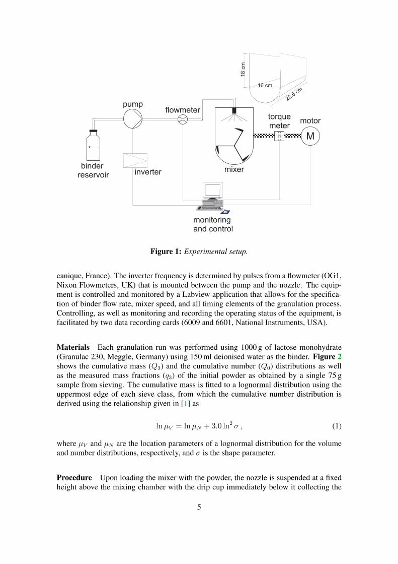
Experimental setup The equipment set-up that was used is shown in Figure 1. The ex-periments were performed using a horizontal axis 5 litre ploughshare mixer (Kemeutec)which is described in detail in Jones and Bridgwater [23]. The mixer shaft is driven by avariable speed DC motor with a torque meter (DRBK-20-n, ETH Messtechnik, Germany)mounted between the shaft and the motor. The mixing chamber is enclosed by a transpar-ent plastic shield, the top of which has an aperture for a nozzle and a drip cup which isconnected to a peristaltic pump (model DBP 764, Dylade Fresenius, UK).

The binder is drawn from a reservoir by a magnetic drive gear pump (model DG.19,Tuthill Corporation, USA) to a single fluid nozzle (model 121, orifice � 0.5 mm, 60 ◦

spray angle, Dusen-Schlick, Germany) which is suspended at a fixed height above thepowder bed. The pump speed is controlled by an inverter (model Altivar 31, Teleme-

4

inverter mixer

monitoringand control

torquemeter

binderreservoir

pumpflowmeter

M

motor

Figure 1: Experimental setup.

canique, France). The inverter frequency is determined by pulses from a flowmeter (OG1,Nixon Flowmeters, UK) that is mounted between the pump and the nozzle. The equip-ment is controlled and monitored by a Labview application that allows for the specifica-tion of binder flow rate, mixer speed, and all timing elements of the granulation process.Controlling, as well as monitoring and recording the operating status of the equipment, isfacilitated by two data recording cards (6009 and 6601, National Instruments, USA).

Materials Each granulation run was performed using 1000 g of lactose monohydrate(Granulac 230, Meggle, Germany) using 150 ml deionised water as the binder. Figure 2shows the cumulative mass (Q3) and the cumulative number (Q0) distributions as wellas the measured mass fractions (q3) of the initial powder as obtained by a single 75 gsample from sieving. The cumulative mass is fitted to a lognormal distribution using theuppermost edge of each sieve class, from which the cumulative number distribution isderived using the relationship given in [1] as

lnµV = lnµN + 3.0 ln2 σ , (1)

where µV and µN are the location parameters of a lognormal distribution for the volumeand number distributions, respectively, and σ is the shape parameter.

Procedure Upon loading the mixer with the powder, the nozzle is suspended at a fixedheight above the mixing chamber with the drip cup immediately below it collecting the

5

0.0

0.4

0.8

Particle size [µm]

Per

cent

age

[−]

10 100

Q3 Exp.Q3 log fitQ0 log fitq3 Exp.

Figure 2: Size distributions of powder used in experiments (lactose monohydrate). Nor-malised cumulative mass, Q3, fit to lognormal distribution; derived numbersize distribution, Q0, with lognormal fit distribution of µpsd = 38.93 σpsd=1.60and fraction of mass, q3.

6

binder flow. After two minutes of dry mixing to aerate the powder, the drip cup is re-moved. When the allotted amount of time for the binder addition has passed, the binderstream is automatically shut off by the controller program and the drip cup is replacedunder the nozzle to prevent any additional droplets from reaching the powder bed. Themixer continues to run at the specified speed until the desired amount of time has elapsed.

The resulting product is removed from the mixer and distributed onto metal trays. Thetrays are placed in a drying cabinet (INC 95SF, Genlab, UK) at 50 ◦C with 55 ◦C desig-nated as the overheat temperature, until no significant change in mass is recorded. Thedried product is recombined and samples for analysis are chosen by putting the entiredried product through a sample splitter until a sample between 50 – 90 g is obtained.

Particle size analysis is performed by sieving. Three tiers, each consisting of six sievesand a bottom pan, were constructed using a

√2 progression from 53 – 16000 µm. Each

tier was subjected to 25 minutes of vibration at approximately 1.5 mm amplitude on asieve shaker (model EVL1, Endecotts, UK). Material in each of the sieves, as well as thebottom pan, was weighed and recorded giving 19 mass measurements.

Potential experimental errors A preliminary granulation run was performed in orderto detect any major sources of error or sub-optimal procedures. As a result, the binder flowcontrol was reconfigured and is measurably accurate to within ± 1 ml/min. Prior to eachgranulation run, the binder flow rate was tested for 150 ml of binder over the specified ad-dition time. The granulation run was performed using control conditions that successfullyproduced 150 ml± 2 ml of binder under the relevant process conditions immediately priorto each granulation run. The sieving analysis of the preliminary run allowed the selectionof an appropriate range of sieves. The balances that were employed for the material andsieving measurements (XB 3200C, Precisa and 2200 P, Sartorius) are accurate to 0.01 g.The motor controller, in conjunction with the torque meter, monitors and adjusts the im-peller speed at least once per second. Analysis of the recorded measurements during thegranulation runs indicate that the average deviation from the specified speed for all thegranulation runs is less than ± 2 rpm. Figure 3 shows the measured speed values for anarbitrarily chosen set of experimental conditions (A4). As can be seen, while there arefluctuations, the speed does stay centred on the designated value, in this case 120 rpm,with the most extreme deviations at the beginning of the experimental run.

The process conditions were selected with a view towards having statistically detectableresults with varied process conditions. Based on previously published results [4, 39, 44,46], it was decided to fix all remaining experimental conditions, including the binder topowder ratio of 150 ml:1000 g, and to use:

1. Binder addition flow rates of 50, 75 and 100 ml/min (flow rate);

2. Mixer speed rates of 120, 180 and 240 rpm (impeller speed); and

3. Allowing the mixer to continue after all the binder had been added for 5, 10 and 15minutes (massing time).

As a complete set of experiments would involve 33 granulation runs with associated par-ticle analysis, it was decided to use a fractional factorial design of 33−1. With this choice

7

0 200 400 600 800 1000 1200

6080

100

120

140

Sample number [−]

Spe

ed [r

pm]

Aeration

Binder addition

Massing time

Figure 3: Measured speed of mixer during experiment A4. White region denotes aera-tion stage (2 minutes). Blue region denotes liquid addition stage (90 seconds).Green region denotes massing stage (10 minutes).

8

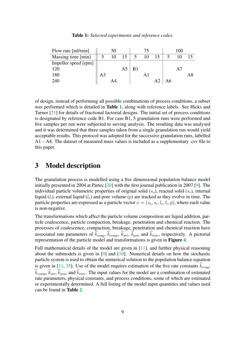
Table 1: Selected experiments and reference codes.

Flow rate [ml/min] 50 75 100Massing time [min] 5 10 15 5 10 15 5 10 15Impeller speed [rpm]120 A5 B1 A7180 A3 A1 A8240 A4 A2 A6

of design, instead of performing all possible combinations of process conditions, a subsetwas performed which is detailed in Table 1, along with reference labels. See Hicks andTurner [21] for details of fractional factorial designs. The initial set of process conditionsis designated by reference code B1. For case B1, 5 granulation runs were performed andfive samples per run were subjected to sieving analysis. The resulting data was analysedand it was determined that three samples taken from a single granulation run would yieldacceptable results. This protocol was adopted for the successive granulation runs, labelledA1 – A8. The dataset of measured mass values is included as a supplementary .csv file tothis paper.

3 Model description

The granulation process is modelled using a five dimensional population balance modelinitially presented in 2004 at Partec [20] with the first journal publication in 2007 [9]. Theindividual particle volumetric properties of original solid (so), reacted solid (sr), internalliquid (li), external liquid (le) and pore volume (p) are tracked as they evolve in time. Theparticle properties are expressed as a particle vector x = (so, sr, le, li, p), where each valueis non-negative.

The transformations which affect the particle volume composition are liquid addition, par-ticle coalescence, particle compaction, breakage, penetration and chemical reaction. Theprocesses of coalescence, compaction, breakage, penetration and chemical reaction haveassociated rate parameters of kcoag, kcomp, katt, kpen and kreac, respectively. A pictorialrepresentation of the particle model and transformations is given in Figure 4.

Full mathematical details of the model are given in [11], and further physical reasoningabout the submodels is given in [9] and [10]. Numerical details on how the stochasticparticle system is used to obtain the numerical solution to the population balance equationis given in [11, 35]. Use of the model requires estimation of the five rate constants kcoag,kcomp, katt, kpen, and kreac. The input values for the model are a combination of estimatedrate parameters, physical constants, and process conditions, some of which are estimatedor experimentally determined. A full listing of the model input quantities and values usedcan be found in Table 2.

9

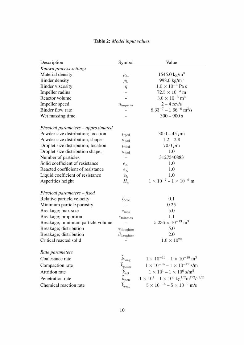
Table 2: Model input values.

Description Symbol ValueKnown process settingsMaterial density ρso 1545.0 kg/m3

Binder density ρle 998.0 kg/m3

Binder viscosity η 1.0× 10−3 Pa sImpeller radius - 72.5× 10−3 mReactor volume - 3.0× 10−3 m3

Impeller speed nimpeller 2 – 4 rev/sBinder flow rate - 8.33−7 – 1.66−6 m3/sWet massing time - 300 – 900 s

Physical parameters – approximatedPowder size distribution; location µpsd 30.0 – 45 µmPowder size distribution; shape σpsd 1.2 – 2.8Droplet size distribution; location µdsd 70.0 µmDroplet size distribution shape; σdsd 1.0Number of particles - 3127540883Solid coefficient of resistance eso 1.0Reacted coefficient of resistance esr 1.0Liquid coefficient of resistance eli 1.0Asperities height Ha 1× 10−7 – 1× 10−6 m

Physical parameters – fixedRelative particle velocity Ucol 0.1Minimum particle porosity - 0.25Breakage; max size νmax 5.0Breakage; proportion νminmax 1.1Breakage; minimum particle volume - 5.236× 10−13 m3

Breakage; distribution αdaughter 5.0Breakage; distribution βdaughter 2.0Critical reacted solid - 1.0× 1020

Rate parametersCoalesance rate kcoag 1× 10−14 – 1× 10−10 m3

Compaction rate kcomp 1× 10−15 – 1× 10−12 s/mAttrition rate katt 1× 101 – 1× 106 s/m5

Penetration rate kpen 1× 101 – 1× 106 kg1/2m7/2/s3/2

Chemical reaction rate kreac 5× 10−16 – 5× 10−9 m/s

10

solid original

external liquid

pores

internal liquid

solid reacted

breakage

compaction penetration

reactioncoalescence

liquid addition

Figure 4: Particle model and transformations in granulation process.

3.1 Coalescence submodel

Of particular interest for our study is the model’s implementation of coalescence. Asdescribed in [9] the rate parameter kcoag is defined such that the collision rate of twoparticles x′ and x′′ is given by the kernel:

K(x′, x′′) = nimpeller kcoag , (2)

with input parameters nimpeller (impeller speed) and kcoag (rate constant). Thus, the num-ber of collisions which may result in coalescence is controlled by the estimated rate con-stant and the impeller speed. However, the occurrence of successful coalescence eventsbetween two particles, once such a collision has taken place, is governed by the Stokescriterion. This is implemented under the assumption that the particle is spherical, with theparticle radius given by

R(x) =3

√3

4 πv(x) , (3)

where v(x) is the particle volume calculated as:

v(x) = so + sr + le + li + p. (4)

Further, with the assumption that the densities of the liquids and the reacted solid are thesame,

ρle = ρli = ρsr , (5)

the particle mass takes the form

m(x) = ρso so + ρle (sr + li + le) , (6)

where ρso and ρle are input parameters.

11

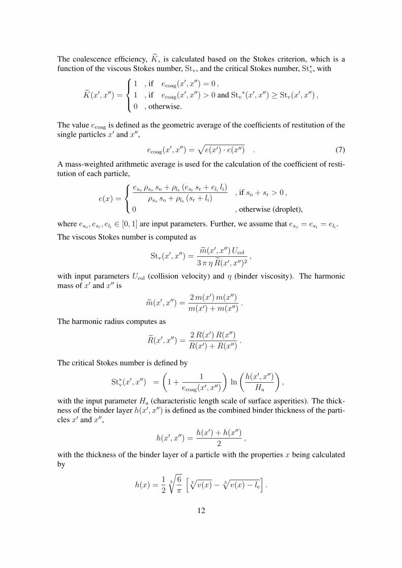
The coalescence efficiency, K, is calculated based on the Stokes criterion, which is afunction of the viscous Stokes number, Stv, and the critical Stokes number, St∗v, with

K(x′, x′′) =

1 , if ecoag(x

′, x′′) = 0 ,

1 , if ecoag(x′, x′′) > 0 and Stv

∗(x′, x′′) ≥ Stv(x′, x′′) ,

0 , otherwise.

The value ecoag is defined as the geometric average of the coefficients of restitution of thesingle particles x′ and x′′,

ecoag(x′, x′′) =

√e(x′) · e(x′′) . (7)

A mass-weighted arithmetic average is used for the calculation of the coefficient of resti-tution of each particle,

e(x) =

eso ρso so + ρle (esr sr + eli li)

ρso so + ρle (sr + li), if so + sr > 0 ,

0 , otherwise (droplet),

where eso , esr , eli ∈ [0, 1] are input parameters. Further, we assume that eso = esr = eli .

The viscous Stokes number is computed as

Stv(x′, x′′) =

m(x′, x′′)Ucol

3π η R(x′, x′′)2,

with input parameters Ucol (collision velocity) and η (binder viscosity). The harmonicmass of x′ and x′′ is

m(x′, x′′) =2m(x′)m(x′′)

m(x′) +m(x′′).

The harmonic radius computes as

R(x′, x′′) =2R(x′)R(x′′)

R(x′) +R(x′′).

The critical Stokes number is defined by

St∗v(x′, x′′) =

(1 +

1

ecoag(x′, x′′)

)ln

(h(x′, x′′)

Ha

),

with the input parameter Ha (characteristic length scale of surface asperities). The thick-ness of the binder layer h(x′, x′′) is defined as the combined binder thickness of the parti-cles x′ and x′′,

h(x′, x′′) =h(x′) + h(x′′)

2,

with the thickness of the binder layer of a particle with the properties x being calculatedby

h(x) =1

23

√6

π

[3√v(x)− 3

√v(x)− le

].

12

3.2 Evolution of particle ensemble

The initial state of the system is a set of 2treesize particles of the form

x = (so, 0, 0, 0, 0)

where treesize is an integer input parameter that determines the maximum number ofparticles to be tracked by the model. Initially, when time is zero, all the particles in theensemble are comprised only of original solid. The volumetric quantities of the originalsolid is initially populated by randomly selecting values from a lognormal distributioncharacterised by two input parameters, a location parameter µpsd and a shape parameterσpsd.

The implementation of the model is such that when a coalescence event occurs, two par-ticles are selected from the ensemble to create a single new particle. A breakage eventcauses a single particle to split and its volume is randomly distributed according to a betadistribution between the two resultant entries in the particle ensemble. When the popula-tion becomes too low, less than or equal to 3/8 of 2treesize, the population is doubled, orin other words a duplicate particle for every member of the particle ensemble is insertedinto the ensemble. If the particle ensemble becomes full, a randomly selected particle isremoved [11].

3.3 Post-processing

The model returns a set of particles described by the five element vector; however we needto convert the results of the simulation to a form which directly relates to our experimentalresults.

For each particle, x, in the final ensemble, the particle mass is calculated using Equation 5under the assumption that, due to a drying process, all of the liquid has been removed,i.e. li = le = 0. The total volume is calculated using Equation 4. From the volume wecalculate R(x), the radius of the particle, using Equation 3. By doubling R(x) we obtaina diameter for the particle, which can be used as a sieving diameter. All the particles inthe final ensemble can then be sorted into sieve classes identical to the experimental data.The total mass in each sieve class is calculated by summing the mass for all particlessorted into a given sieve class. From these values, an empirical cumulative distribution iscalculated, as with the physical system.

4 Parameter estimation methodology

In the first instance, the model has five rate parameters which need to be estimated usingthe experimental data. Accomplishing this requires a series of decisions with respect tothe methods available and the tolerances necessary. In this implementation, one beginsby defining the boundaries of the model parameter space and evaluating the model atpoints sampled from that space. Then one examines the set of evaluated points, seekingan optimum point or region. In this paper we make use of Sobol sequences to sample the

13

multi-dimensional bounded parameter space. With the sets of model evaluations, we usea variety of criteria to assess the performance of the model in comparison to the experi-mental results and to draw inferences from its behaviour. The ‘best’ Sobol point of the setis determined by some objective function; in this case specifically we use least squares,or the smallest Euclidian distance between the experimental results and the simulation,as the objective function for various methods of quantifying the results. In this sectionthe methodology used to define the parameter space, generate the set of Sobol points andevaluate the model performance is detailed.

4.1 Parameter space

A number of factors must be considered when defining the parameter space. Theoreti-cally, the rate parameters can range either from 0 to ∞, or from 0 to 1, but the numberof collision events determined by the rates kcoag and katt can limit the feasible ranges.The run-time of the model increases with respect to these parameters and can becomeprohibitively expensive when the rates become too large. A preliminary study of the runtimes yielded guidelines for the parameter space which will keep the run times feasible.Further, tracking a larger number of particles significantly increases the model run time.Based on the results published for this model in [11] and a preliminary convergence study,each model evaluation consists of 64 repetitions, each based on a different random num-ber seed, and tracks 4096 individual particles. Thus, the boundaries for the rates are notonly defined by the requirements of the physical system, but also by practical concernsdetermined by the evaluation time and model convergence.

Additionally, a smaller parameter space will yield a finer resolution for the same numberof sampling points. The final parameter space used in this paper was established by aniterative process. Initially, a set of parameter boundaries was selected based on the run-time requirements and the model was evaluated over that range. The initial parameterspace was deliberately chosen to be large so that it could be reduced appropriately. Thatspace was then reduced based on a comparison of the experimental data and the results ofthe model. The reductions were implemented to eliminate regions which were obviouslypoor choices, e.g. when the coagulation rate was so small that particles were only beinggenerated in the smallest five sieve classes. This process was repeated with the reducedparameter space until it was decided further reductions could possibly eliminate viableregions.

4.2 Sobol sequences

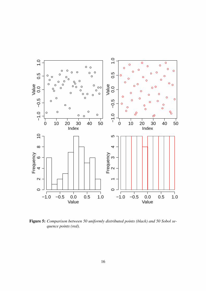
Once the parameter boundaries are fixed, a set of model evaluations is created using Sobolsequences. Sobol sequences, initially developed by I.M. Sobol in 1973, are quasi-randomlow-discrepancy sequences [7]. They are constructed in such a way as to generate a se-quence of numbers which are both quasi-random and well-spaced as well as being compu-tationally inexpensive. As the sequence progresses, the resolution becomes increasinglyfine. To illustrate, Figure 5 shows fifty points both randomly generated and generatedfrom a Sobol sequence over the same region. It can be seen in the histograms that the

14

Sobol points fill the space more evenly. For this application, we use the Sobol points tosample the parameter space. By taking advantage of the quasi-random nature of Sobolpoints, we can sample from any bounded range by the simple expedient of treating it asan additional model parameter.

For each iteration in the model fitting process, 2,000 to 4,000 points were generated usinga Sobol sequence. The points are mapped to the parameter space using the scheme de-scribed in [32] with a logarithmic transformation for parameters which vary over ordersof magnitude and a linear transformation otherwise. The number of Sobol points wasdetermined by the rough method of assessing the improvement, or lack thereof, in the ob-jective functions when the number of points was doubled, beginning with 500 points. Bythis method a baseline of 2,000 points was established for the lower dimensional cases,which was increased to 4,000 points for the highest dimensional case. In effect this pro-cess means that for each Sobol point a parameter value is quasi-randomly selected fromthe parameter space. Then the model is evaluated for the 9 experimental cases at the se-lected set of parameter values and the objective function is calculated. The ‘best’ set ofparameter values is designated by the smallest objective function value calculated over allof the sampled points. To give a sense of the model runtimes required, one of the final2000 Sobol point runs required 32 CPUs (in parallel) approximately 12 hours to complete18000 individual model evaluations.

4.3 Additional parameters of interest

While the model requires estimation of the five rate parameters, it is initially assumedthat the remaining physical parameters are fixed values. However, while attempting tosimulate the experimental data, the model demonstrated sensitivity to two aspects of thepowder characterisation.

4.3.1 Height of asperities

Regardless of how we choose to quantify the height of asperities for a given powder,any single value characterisation will perforce be an approximation, as different particleswill have asperities of varying heights. For this powder, as we have no experimentaldata to inform our decisions, we begin with an initial estimate of 1.0µm for the heightof asperities. However, as any single value is an approximation which would need to beadjusted until it achieved some abstract state of correctness, we propose instead to definea range based on ‘reasonable’ physical boundaries which will be refined by the behaviourof the model. The performance of the model with respect to particle size growth suggeststhat 1.0 µm belongs at the upper bound of the range, thus we choose to explore a range of0.1–1.0 µm.

Further, by nature of the Sobol sequences, we can easily sample from this range by treatingit as a sixth parameter. The model continues to use a single value characterisation for theheight of asperities for each set of rates; however that value is quasi-randomly selectedfrom the range. With the addition of a sixth parameter, 2,000 Sobol points were found tobe adequate to sample the parameter space.

15

0 10 20 30 40 50

−1.

0−

0.5

0.0

0.5

1.0

Index

Val

ue

0 10 20 30 40 50−1.

0−

0.5

0.0

0.5

1.0

Index

Val

ue

Value

Fre

quen

cy

−1.0 −0.5 0.0 0.5 1.0

02

46

810

Value

Fre

quen

cy

−1.0 −0.5 0.0 0.5 1.0

01

23

45

Figure 5: Comparison between 50 uniformly distributed points (black) and 50 Sobol se-quence points (red).

16

4.3.2 Initial powder size distribution

The initial powder size distribution is based on experimental data as discussed in Sec-tion 2. The model inputs are µpsd = exp(µN) and σpsd = exp(σ) where µN and σdefine a lognormal curve based on the estimated number distribution of powder sievingdata. However, µN and σ are derived from experimental measurements and contain un-certainty, both from the measurement technique and the curve-fitting process. Given thisuncertainty, we construct ranges around the experimentally determined input values andsample from those ranges with Sobol points in the same manner used with the height ofasperities. By beginning with large ranges for both parameters based around the initialestimates and reducing them to viable regions, we have final ranges of 20 – 45 µm forµpsd and 1.2 – 2.0 for σpsd with the sieving based estimates of 38.93 and 1.60, respec-tively. This is equivalent to 2.99 – 3.80 for µN and 0.182 – 0.693 for σ with sievingdata estimates of 3.66 and 0.47, respectively. With the inclusion of these two additionalparameters, we generate 4,000 Sobol points in an eight-dimensional space.

4.4 Criteria for objective function

In the experimental portion of the work, we obtain a vector of sieving measurementswhich describe the end-product of the particle size distribution. There are many waysto express these results quantitatively and we shall use more than one to assess the per-formance of the model. In all cases, as the considered quantities are similar in order ofmagnitude, we shall use the Euclidian distance as the objective function. To accomplishthis, we select an observable quantity f , e.g. the empirical geometric mean particle size,and then for each model evaluation we calculate a value:

OF =

√√√√ N∑j=1

M∑i=1

(f simij − f

expij )2 , (8)

where N is the number of experimental runs and M is the number of responses for eachcriterion, f sim is the response from the simulation and f exp is the response from the ex-perimental data. In this manner we obtain a numeric expression of the fit of the modelto the experimental data. The single variate functions that we will use for f(x) are theempirical geometric mean particle size and the empirical variance. Further, we shall usethe multivariate characterisations of categorical quantiles and empirical cumulative distri-bution. For all of these functions, the best parameter set is considered to be the set withthe smallest objective function value.

4.4.1 Empirical cumulative distribution

The values for this objective function are determined directly from the experiments andthe post-processing of the model. The vectors are derived from mass fractions that areexpressed as a N dimensional vector d, where N is the number of sieve classes. The

17

density can also be physically interpreted as the percentage of mass that is found in eachsieve class. These values are calculated as:

di =mi∑Nj=1mj

, (9)

where mi is the mass measured in the ith sieve class by sieving or postprocessing.

From this point, we convert the values into an empirical cumulative distribution functionby summing all fractions of mass that are smaller than a given sieve class. This is equiva-lent to sieving measurements in terms of proportions of material that have passed throughany given sieve aperture. The empirical distribution function, D, is also a N dimensionalvector, which is calculated directly from the mass fractions as:

Di =i∑

j=1

dj , (10)

where i = 1, . . . , N .

4.4.2 Empirical geometric mean particle size

The empirical geometric mean particle size, Mg, is a single value expression used todescribe the particle size distribution. In this context, we use the geometric mean particlesize, wherein we transform the sieve aperture values, x, by taking the natural log. Thistransformation is used so that the larger particle size classes are not disproportionatelyrepresented. In the sieve series that we use, the range of the sieve classes is 53 µm –16000 µm which, by taking the natural log, transforms into 3.97 – 9.68, i.e. x′ = ln(x).The empirical geometric mean particle size is calculated by first multiplying the densityby the transformed sieve class and then taking the exponential of the summed the results:

Mg = exp

(N∑i=1

dix′i

), (11)

where each di is the ith element of the N dimensional density function and x′i is the upperbound of the ith sieve class under the natural log transformation.

4.4.3 Empirical variance

The variance, V ar is a single value expression of the spread of the resultant particle sizedistribution. For this value, we shall use the untransformed sieve class values, i.e. usingthe arithmetic means. The variance is calculated as:

V ar =N∑i=1

dix2i −

(N∑i=1

dixi

)2

(12)

18

where each di is the ith element of theN -dimensional density function and xi is the upperbound of the ith sieve class.

4.4.4 Categorical percentile

In powder studies, one of the more popular methods of describing the materials is by usingpercentiles, specifically the 10th, 50th and 90th percentiles. However, to analyse our datausing these values some choices need to be made, as we are using categorical data. Oneway to quantify a percentile value is based on the category, or sieve class. If one uses anindex as the category identifier, then one can find the category where the desired quantilebelongs. For example: if the ECDF is: 0.0077, 0.028, 0.083, 0.2155, 0.3993, 0.5953,0.7683, 0.8947, 0.9778, 0.9915, 1.0; then the 10th percentile is in the 3rd sieve class,the 50th percentile is in the 5th sieve class and the 90th is in the 8th sieve class. Thisprocess gives a vector which expresses how far away from the experimental sieve classesthe model results are. In addition to the usual objective function, we can also sum thethree numbers to get a deviation score for all three measurements. For example if theexperimental data has [3, 6, 9] as the 10th, 50th and 90th percentiles, respectively, andthe model produces [2, 4, 11]; the differences are [1, 2, 2], which gives 5 for that set ofexperimental conditions.

5 Results

5.1 Model results

The final, iteratively determined, parameter space is detailed below in Table 3. We per-form runs of 2,000 to 4,000 Sobol points on this space with the model under three differentsituations. The selection of the three parameter sets is based on sensitivities observed dur-ing preliminary model evaluations. The first model configuration uses 2,000 Sobol pointsfor the five rate parameters with fixed values for the height of asperities and for the twoparameters, µpsd and σpsd, that determine the initial powder size distribution. The secondalso uses 2,000 Sobol points and incorporates the height of asperities, Ha, as a sixth pa-rameter while maintaining fixed values for µpsd and σpsd. The third situation uses 4,000Sobol points for eight parameters, µpsd and σpsd in addition to the five rate parametersand Ha. The ranges for the µpsd, σpsd and Ha are expansions upon the five-parametersetup based on the models behaviour with respect to the fixed values of 38.93µm, 1.60and 1× 10−6m. In the following discussion, the focus will be upon the behaviour of theseparameters and the rate parameter for kcoag, as these parameters were observed exhibit themost influence on the results.

5.2 Experimental results

The mass fraction vector, q3, is obtained directly from laboratory measurements. Theempirical cumulative distribution, Q3, is then calculated by Equation 10 for each sample,

19

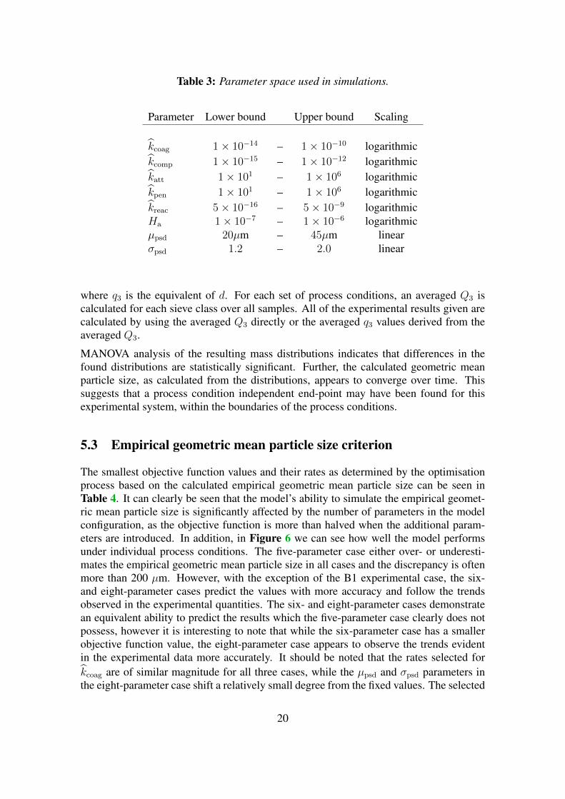
Table 3: Parameter space used in simulations.

Parameter Lower bound Upper bound Scaling

kcoag 1× 10−14 – 1× 10−10 logarithmickcomp 1× 10−15 – 1× 10−12 logarithmickatt 1× 101 – 1× 106 logarithmickpen 1× 101 – 1× 106 logarithmickreac 5× 10−16 – 5× 10−9 logarithmicHa 1× 10−7 – 1× 10−6 logarithmicµpsd 20µm – 45µm linearσpsd 1.2 – 2.0 linear

where q3 is the equivalent of d. For each set of process conditions, an averaged Q3 iscalculated for each sieve class over all samples. All of the experimental results given arecalculated by using the averaged Q3 directly or the averaged q3 values derived from theaveraged Q3.

MANOVA analysis of the resulting mass distributions indicates that differences in thefound distributions are statistically significant. Further, the calculated geometric meanparticle size, as calculated from the distributions, appears to converge over time. Thissuggests that a process condition independent end-point may have been found for thisexperimental system, within the boundaries of the process conditions.

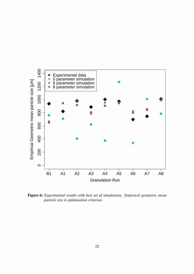
5.3 Empirical geometric mean particle size criterion

The smallest objective function values and their rates as determined by the optimisationprocess based on the calculated empirical geometric mean particle size can be seen inTable 4. It can clearly be seen that the model’s ability to simulate the empirical geomet-ric mean particle size is significantly affected by the number of parameters in the modelconfiguration, as the objective function is more than halved when the additional param-eters are introduced. In addition, in Figure 6 we can see how well the model performsunder individual process conditions. The five-parameter case either over- or underesti-mates the empirical geometric mean particle size in all cases and the discrepancy is oftenmore than 200 µm. However, with the exception of the B1 experimental case, the six-and eight-parameter cases predict the values with more accuracy and follow the trendsobserved in the experimental quantities. The six- and eight-parameter cases demonstratean equivalent ability to predict the results which the five-parameter case clearly does notpossess, however it is interesting to note that while the six-parameter case has a smallerobjective function value, the eight-parameter case appears to observe the trends evidentin the experimental data more accurately. It should be noted that the rates selected forkcoag are of similar magnitude for all three cases, while the µpsd and σpsd parameters inthe eight-parameter case shift a relatively small degree from the fixed values. The selected

20

Table 4: Objective function and best estimated parameters where empirical geometricmean particle size is selection criterion. Fixed parameters are in bold.

5 parameters 6 parameters 8 parameters

Objective function 1079.35 362.54 372.01

kcoag 2.90× 10−13 1.72× 10−13 2.13× 10−13

kcomp 1.01× 10−13 2.14× 10−14 2.89× 10−13

katt 24335 1833 236

kpen 27 994394 871336

kreac 1.08× 10−14 1.37× 10−11 7.83× 10−10

Ha 1 × 10−6 2.52× 10−7 3.40× 10−7

µpsd 38.93µm 38.93µm 31.7µmσpsd 1.60 1.60 1.62

µpsd has a slight downward shift and σpsd increases slightly. The selected Ha parameterhowever, has a significant and similar decrease from the five-parameter fixed value forboth alternate cases. This suggests that the Ha is significant with respect to this form ofdescribing the particle size distribution and our initial guess of 1.0 µm is too large.

5.4 Empirical variance criterion

The smallest objective functions and rates that were selected by optimising the varianceof the resulting particle size distribution can be seen in Table 5. Interestingly, while allthe objective functions are of a similar order of magnitude, the five-parameter case ismarginally smaller than the others and the six parameter case is slightly smaller than theeight parameter case. Further, in Figure 7 we can see that all cases are largely equal inperformance, with the A2 experimental case being the exception to the model followingthe experimental trends. The rates selected by the objective functions should be noted,insofar that the chosen kcoag parameters are two orders of magnitude larger than for thegeometric mean particle size. This can be understood as a result of the method by whichthe variance is calculated such that large particle sizes will have more influence. Thissuggests that in order to optimise the variance all selected cases generate larger particlesthen when optimising the empirical geometric mean particle size. Further, note that againthe six- and eight-parameter selection for Ha is similar and larger than for the geometricmean particle size. Interestingly, taken together with the rates, this indicates that morecoagulation events are happening, with a lower success rate than with the geometric meanparticle size. Additionally, we see a further downward shift in the value for µpsd and afurther increase in σpsd. This indicates that the selected initial distribution is centred ata lower value, but is more widely spread than with the fixed conditions, a by-product ofwhich is that the initial powder would have a larger variance than with the fixed values.

21

020

040

060

080

010

0012

0014

00

Granulation Run

Em

piric

al G

eom

etric

mea

n pa

rtic

le s

ize

[µm

]

B1 A1 A2 A3 A4 A5 A6 A7 A8

Experimental data5 parameter simulation6 parameter simulation8 parameter simulation

Figure 6: Experimental results with best set of simulations. Empirical geometric meanparticle size is optimisation criterion.

22

Table 5: Objective function and best estimated parameters where empirical variance isselection criterion. Fixed parameters are in bold.

5 parameters 6 parameters 8 parameters

Objective function 11541339 12675168 13959977

kcoag 3.44× 10−11 5.44× 10−11 9.59× 10−11

kcomp 3.13× 10−15 9.04× 10−15 4.76× 10−14

katt 1895 24 980

kpen 965 13260 24853

kreac 7.58× 10−16 1.83× 10−12 9.10× 10−14

Ha 1 × 10−6 5.99× 10−7 5.60× 10−7

µpsd 38.93µm 38.93µm 29.7µmσpsd 1.60 1.60 1.84

Granulation Run

Em

piric

al v

aria

nce

in p

artic

le s

ize

[µm

]

B1 A1 A2 A3 A4 A5 A6 A7 A8

5×

106

5×

107

Experimental data5 parameter simulation6 parameter simulation8 parameter simulation

Figure 7: Experimental results with best set of simulations. Empirical variance is opti-misation criterion.

23

5.5 Categorical percentile size criterion

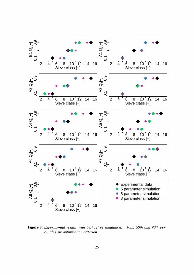
The results of the objective function and the rates that were selected by the optimisationprocess based on the 10th, 50th and 90th percentiles, when treated as strictly categoricaldata, can be seen in Table 6. Additionally, the absolute distance between the simulatedsieve classes and the experimental points is included. The objective function decreasesslightly with the addition of the sixth parameter and is decreased by 1/3 for the eight-parameter case when compared to the five-parameter case. In Figure 8 we can againsee that for all experimental cases, the five-parameter system is consistently over- or un-dersized. We can observe a slight improvement overall with the six-parameter case, butin most experimental cases the behaviour for the five- and six-parameters cases is sim-ilar. Additionally, by the counts portrayed by the objective function values and in thefigures, one can see that while the eight-parameter case may deviate one, two, or, on threeoccasions, 3 sieve classes from the experimental results, the five and six-parameter con-figurations deviate by 3 sieve classes at least five times and by 4-5 sieve classes multipletimes. Further, note that while the 10th percentile is exactly matched by all parameterconfigurations for three sets of process conditions, the 90th percentile is only simulatedexactly in one instance by the 8 parameter case. While the eight-parameter case deviatesby one or two sieve classes from the 90th percentile class, the five- and six-parametercases frequently deviate by 3 or more classes.

With respect to the selected rates, while the selection for kcoag has returned the area se-lected by the geometric mean particle size method for the five- and six- parameter con-figurations, the eight-parameter case has remained in the area that was selected by thevariance-based optimisation. This suggests that the parameter values selected for the vari-ance were created an oversized particle size distribution, with respect to the geometricmean particle size, for the five- and six-parameter cases. Further, this suggests that thevalues selected for the geometric mean particle size are not representative of an accuratevariance in all cases. The value for Ha is again increased to a similar degree for the six-and eight-parameter cases, to the point that it only deviates marginally from the fixedvalue for the five-parameter case. Further, we again note that for the eight parameter casethere is a noticeable increase in the σpsd with a minor decrease in the µpsd. Overall, thissuggests that that the shape of the distribution is more significant than its location whenattempting to simulate more complicated assessments of the experimental data.

5.6 Empirical cumulative size distribution criterion

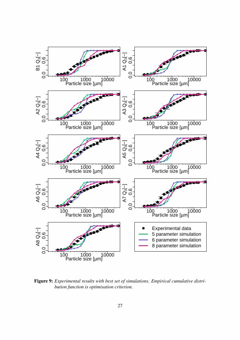
Next, we use a more detailed form of model output. Here, we shall examine the empiricalcumulative size distribution (ECDF) for all of the experimentally measured values. Theobjective function and selected rates are displayed in Table 7, where the same pattern ofdecreasing objective functions is shown for the model configurations. In Figure 9 we candirectly compare how the selected simulated ECDF fits the experimental data. Here wecan see that the shape of the resultant ECDF remains largely the same for the five- andsix-parameter scenarios, and in neither case are they a particularly good fit to the exper-imental results. The five- and six- parameter cases consistently fail to produce particlesin the larger sieve classes and also show a tendency to place an inappropriate amount

24

Sieve class [−]

B1

Q3[

−]

2 4 6 8 10 12 14 16

0.1

0.9

Sieve class [−]

A1

Q3[

−]

2 4 6 8 10 12 14 16

0.1

0.9

Sieve class [−]

A2

Q3[

−]

2 4 6 8 10 12 14 16

0.1

0.9

Sieve class [−]A

3 Q

3[−

]2 4 6 8 10 12 14 16

0.1

0.9

Sieve class [−]

A4

Q3[

−]

2 4 6 8 10 12 14 16

0.1

0.9

Sieve class [−]

A5

Q3[

−]

2 4 6 8 10 12 14 16

0.1

0.9

Sieve class [−]

A6

Q3[

−]

2 4 6 8 10 12 14 16

0.1

0.9

Sieve class [−]

A7

Q3[

−]

2 4 6 8 10 12 14 16

0.1

0.9

Sieve class [−]

A8

Q3[

−]

2 4 6 8 10 12 14 16

0.1

0.9 Experimental data

5 parameter simulation6 parameter simulation8 parameter simulation

Figure 8: Experimental results with best set of simulations. 10th, 50th and 90th per-centiles are optimisation criterion.

25

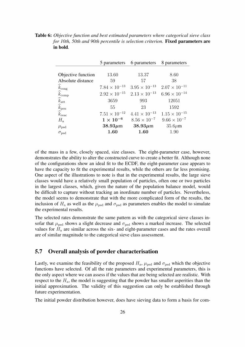
Table 6: Objective function and best estimated parameters where categorical sieve classfor 10th, 50th and 90th percentile is selection criterion. Fixed parameters arein bold.

5 parameters 6 parameters 8 parameters

Objective function 13.60 13.37 8.60Absolute distance 59 57 38

kcoag 7.84× 10−13 3.95× 10−13 2.07× 10−11

kcomp 2.92× 10−15 2.13× 10−13 6.96× 10−14

katt 3659 993 12051

kpen 55 23 1592

kreac 7.51× 10−12 4.41× 10−13 1.15× 10−15

Ha 1 × 10−6 8.56× 10−7 9.66× 10−7

µpsd 38.93µm 38.93µm 35.6µmσpsd 1.60 1.60 1.90

of the mass in a few, closely spaced, size classes. The eight-parameter case, however,demonstrates the ability to alter the constructed curve to create a better fit. Although noneof the configurations show an ideal fit to the ECDF, the eight-parameter case appears tohave the capacity to fit the experimental results, while the others are far less promising.One aspect of the illustrations to note is that in the experimental results, the large sieveclasses would have a relatively small population of particles, often one or two particlesin the largest classes, which, given the nature of the population balance model, wouldbe difficult to capture without tracking an inordinate number of particles. Nevertheless,the model seems to demonstrate that with the more complicated form of the results, theinclusion of Ha as well as the µpsd and σpsd as parameters enables the model to simulatethe experimental results.

The selected rates demonstrate the same pattern as with the categorical sieve classes in-sofar that µpsd shows a slight decrease and σpsd shows a marked increase. The selectedvalues for Ha are similar across the six- and eight-parameter cases and the rates overallare of similar magnitude to the categorical sieve class assessment.

5.7 Overall analysis of powder characterisation

Lastly, we examine the feasibility of the proposed Ha, µpsd and σpsd which the objectivefunctions have selected. Of all the rate parameters and experimental parameters, this isthe only aspect where we can assess if the values that are being selected are realistic. Withrespect to the Ha, the model is suggesting that the powder has smaller asperities than theinitial approximation. The validity of this suggestion can only be established throughfuture experimentation.

The initial powder distribution however, does have sieving data to form a basis for com-

26

0.0

0.6

Particle size [µm]

B1

Q3[

−]

100 1000 10000 0.0

0.6

Particle size [µm]

A1

Q3[

−]

100 1000 10000

0.0

0.6

Particle size [µm]

A2

Q3[

−]

100 1000 10000 0.0

0.6

Particle size [µm]A

3 Q

3[−

]100 1000 10000

0.0

0.6

Particle size [µm]

A4

Q3[

−]

100 1000 10000 0.0

0.6

Particle size [µm]

A5

Q3[

−]

100 1000 10000

0.0

0.6

Particle size [µm]

A6

Q3[

−]

100 1000 10000 0.0

0.6

Particle size [µm]

A7

Q3[

−]

100 1000 10000

0.0

0.6

Particle size [µm]

A8

Q3[

−]

100 1000 10000

Experimental data5 parameter simulation6 parameter simulation8 parameter simulation

Figure 9: Experimental results with best set of simulations. Empirical cumulative distri-bution function is optimisation criterion.

27

Table 7: Objective function and best estimated parameters where empirical cumulativedistribution function is selection criterion. Fixed parameters are in bold.

5 parameters 6 parameters 8 parameters

Objective function 2.16 2.03 1.58

kcoag 2.52× 10−13 1.42× 10−13 3.03× 10−11

kcomp 1.21× 10−15 1.07× 10−14 9.35× 10−15

katt 5364 658 271

kpen 38 28 6530

kreac 2.14× 10−13 6.19× 10−13 9.22× 10−14

Ha 1 × 10−6 6.11× 10−7 8.66× 10−7

µpsd 38.93µm 38.93µm 37.9µmσpsd 1.60 1.60 1.97

parison. In Figure 10 and Figure 11 we can see the model suggested fit lines plottedagainst the experimental mass measurements and the derived lognormal fit lines for thenumber and mass distributions of the initial powder. In all instances, the values selectedfor µpsd were of smaller than the fixed value and found values for σpsd were noticeablylarger. Bearing in mind that the model input values are the number distribution, we canobserve the rightward shift and increased spread of the selected distributions. None ofthe alternative combinations of µpsd and σpsd appear to be unreasonable with respect tothe number distribution, particularly when one considers the mechanical nature of sievinganalysis.

When the selected number distributions are converted into mass distributions, the pro-posed changes become more evident and less credible. With respect to mass, the selecteddistributions range from moderately undersized to markedly larger then the measured val-ues. If one interprets the tendency to select significantly larger values for σpsd and smallervalues for µpsd to indicate that the shape of the distribution is more significant, a value ofµpsd could be selected to remedy this disparity, akin to the values found for the variance.Further, the method of sieving analysis forces us to make a choice as to how to define theparticle size with respect to the data points. In this paper, we have used the uppermostpoint of the sieves for the curve fitting, but using the midpoint or the lower most edge ofthe sieve classes are choices which could also be justified. Either of these choices wouldgenerate a smaller value for µpsd, while maintaining the value for σpsd. However, as thebounds for the model were arbitrarily established, it would be inappropriate to make anyconcrete statement with respect to the powder distribution without experimental verifica-tion.

With these observations, a number of possibilities should be considered. Firstly, theremay be a kinetic mechanism which the model does not possess that causes the disparity.Alternately, if the model does possess the relevant mechanisms, then characterisation ofthe powder by either the sieving data or the lognormal curve is insufficient for the model.

28

Particle size [µm]

Q0

[−]

10 100

0.0

0.2

0.4

0.6

0.8

1.0

Initial Q0 fitEmpirical meanEmpirical varianceQuantiles; classEmpirical CDF

Figure 10: Initial powder number distribution found by various objective functions.

In either case, the suggestion that the shape of the distribution is significantly affectingthe end-product should be investigated. A further complication that should be noted is thedifference, sometimes by orders of magnitude, in the optimal rates selected by the variousobjective functions. While this disparity could result from local minima being found in anon-smooth parameter space, it should be the subject of further study.

6 Conclusions

We have presented a combined experimental and modelling approach to understandingthe wet granulation of lactose powder in a high-shear mixer. Experimental data producedby performing nine wet granulation runs using lactose monohydrate as the initial powderand deionised water as the binder is presented and included as a supplementary .csv file.The granulation runs were performed with variations in impeller speed, massing time andbinder addition rate and then simulated by a population balance model containing fiverate parameters requiring estimation. The rates are estimated by sampling with Sobolsequences over a pre-defined parameter space.

The methodology used to perform the parameter estimation is found to yield useful results.By using Sobol sequences as a means to sample the parameter space, we are able tocreate a map of the parameter space and assess the behaviour of the parameters with

29

0.0

0.2

0.4

0.6

0.8

1.0

Particle size [µm]

Q3

[−]

10 100 1000

Sieving dataInitial Q3 fitEmpirical meanEmpirical varianceQuantiles; classEmpirical CDF

Figure 11: Initial powder mass distribution found by various objective functions.

30

respect to various characterisations of the results. Further, by using the Sobol sequencesin conjunction with ranges that reflect uncertainty in the initial values, we gain insight themodel and which can be related back to the physical system.

A sensitivity study performed using this method reveals two important properties withrespect to the characterisation of the initial powder. First, the model input value thatquantifies the height of the asperities on the particles is found to limit the model’s abil-ity to simulate simple descriptions of the particle size distribution. By allowing the pa-rameter for the height of asperities to vary over a range when estimating the rates, thesimulated particle size distribution agrees well with the experimental one when using asingle value characterisation. However, the absence of experimental measurements forthis value necessitates experimental investigation to ascertain if the values being selectedby the optimisation process are realistic.

Second, the input parameters which describe the initial particle size distribution are foundto significantly affect the distribution of the end product. When the input parameterswhich define the size distribution of the initial powder are allowed to vary, the modeldemonstrates an ability to simulate the experimental empirical size distributions. Of thetwo parameters which characterise the initial distribution, the shape parameter seems to bethe most influential. The fact that these values are initially established by fitting a lognor-mal curve to sieving data suggests that this combination of methods is not appropriate forthis model. Further, these observations raise questions with respect to impact that thesequantities have on the experimental system.

Future work will entail experimental investigation of the properties found to be significantin this study. In particular, the effect on the end product of powders with different initialsize distributions will be studied under identical process conditions. Of most interest is theshape of the initial size distribution, as the sensitivity study suggests that this is the moresignificant factor. Further, a detailed investigation of the initial powder will take placeusing a wide variety of techniques to quantify the height of asperities, such as scanningelectron and atomic force microscopes, and to produce size descriptions of the initialpowder by techniques more sophisticated than sieving, such as laser diffraction.

Acknowledgements

Funding by the EPSRC, grant number EP/I01165X, is gratefully acknowledged.

31

Nomenclature

Roman symbols

� Diameter mm

d Density function [-]di ith element of density function [-]D Cumulative mass function [-]Di ith element of cumulative mass function [-]ecoag Coalescence coefficient of restitution [-]e Particle coefficient of restitution [-]eli Liquid coefficient of resistance [-]eso Solid coefficient of resistance [-]esr Reacted coefficient of resistance [-]f Criteria function [-]f exp Simulation criteria [-]f sim Simulation criteria [-]h Binder thickness mHa Asperities height mkatt Attrition rate parameter sm−5

kcoag Coalesance rate parameter m3

kcomp Compaction rate parameter s/mkpen Penetration rate parameter kg1/2s−3/2m−7/2

K Coalescence collision rate [-]K Coalescence efficiency [-]kreac Chemical reaction rate parameter m/sle Volume of external liquid m3

li Volume of internal liquid m3

m Particle mass kgm Harmonic mass kgmi ith mass measurement [-]M Number of responses [-]Mg Empirical geometric mean particle size [-]nimpeller Impeller speed rev/sN Number of experimental runs [-]OF Objective function [-]p Pore volume m3

Q0 Cumulative number distribution [-]q3 Mass density distribution [-]Q3 Cumulative mass distribution [-]R Particle radius mR Harmonic mean particle radius m

32

rpm Revolutions per minute [-]so Volume of original solid m3

sr Volume of reacted solid m3

Stv∗ Stokes number [-]

Stv Critical Stokes number [-]treesize exponent of 2 for number of particles tracked [-]Ucol Relative particle velocity [-]v Total particle volume m3

V ar Empirical variance [-]xi ith sieve class [-]x′i Natural log of ith sieve class [-]

Greek symbols

αdaughter Breakage; distribution -βdaughter Breakage; distribution -η Binder viscosity Pa sµN Lognormal curve location parameter; number distribution [-]µV Lognormal curve location parameter; volume distribution [-]µdsd Droplet distribution location parameter [-]µpsd Powder distribution location parameter [-]νmax Breakage; max size -νminmax Breakage; proportion -ρle Binder density kg/m3

ρso Material density kg/m3

σ Lognormal curve shape parameter [-]σdsd Droplet distribution shape parameter [-]σpsd Powder distribution shape parameter [-]

33

References

[1] T. Allen. Particle Size Measurement. Chapman and Hall, London, England, 4thedition, 1990.

[2] D. Ameye, E. Keleb, C. Vervaet, J. P. Remon, E. Adams, and D. Massart. Scaling-up of a lactose wet granulation process in Mi-Pro high shear mixers. EuropeanJournal of Pharmaceutical Sciences, 17(4–5):247–251, 2002. doi:10.1016/S0928-0987(02)00218-X.

[3] K. Ax, H. Feise, R. Sochon, M. Hounslow, and A. Salman. Influence of liquidbinder dispersion on agglomeration in an intensive mixer. Powder Technology, 179(3):190–194, 2008. doi:10.1016/j.powtec.2007.06.010.

[4] S. I. F. Badawy, M. M. Menning, M. A. Gorko, and D. L. Gilbert. Effect of processparameters on compressibility of granulation manufactured in a high-shear mixer.International Journal of Pharmaceutics, 198(1):51–61, 2000. doi:10.1016/S0378-5173(99)00445-7.

[5] S. I. F. Badawy, A. S. Narang, K. LaMarche, G. Subramanian, and S. A. Varia.Mechanistic basis for the effects of process parameters on quality attributes in highshear wet granulation. International Journal of Pharmaceutics, 439(1–2):324–333,2012. doi:10.1016/j.ijpharm.2012.09.011.

[6] O. G. Batarseh, D. Nazzal, and Y. Wang. An interval-based metamod-eling approach to simulate material handling in semiconductor wafer fabs.IEEE Transactions on Semiconductor Manufacturing, 23(4):527–537, 2010.doi:10.1109/TSM.2010.2066993.

[7] P. Bratley and B. L. Fox. Algorithm 659–implementing sobols quasirandom se-quence generator. ACM Transactions on Mathematical Software, 14(1):88–100,1988. doi:10.1145/42288.214372.

[8] A. Braumann and M. Kraft. Incorporating experimental uncertainties into multivari-ate granulation modelling. Chemical Engineering Science, 65(3):1088–1100, 2010.doi:10.1016/j.ces.2009.09.063.

[9] A. Braumann, M. J. Goodson, M. Kraft, and P. R. Mort. Modelling and validation ofgranulation with heterogeneous binder dispersion and chemical reaction. ChemicalEngineering Science, 62(17):4717–4728, 2007. doi:10.1016/j.ces.2007.05.028.

[10] A. Braumann, M. Kraft, and P. R. Mort. Parameter estimation in a mul-tidimensional granulation model. Powder Technology, 197(3):196–210, 2010.doi:10.1016/j.powtec.2009.09.014.

[11] A. Braumann, M. Kraft, and W. Wagner. Numerical study of a stochastic par-ticle algorithm solving a multidimensional population balance model for highshear granulation. Journal of Computational Physics, 229(20):7672–7691, 2010.doi:10.1016/j.jcp.2010.06.021.

34

[12] A. Braumann, P. L. W. Man, and M. Kraft. Statistical approximation of the inverseproblem in multivariate population balance modeling. Industrial & EngineeringChemistry Research, 49(1):428–438, 2010. doi:10.1021/ie901230u.

[13] A. Braumann, P. L. W. Man, and M. Kraft. The inverse problem in granulationmodelling – two different statistical approaches. AIChE Journal, 57(11):3105–3121,2011. doi:10.1002/aic.12526.

[14] C. J. Broadbent, J. Bridgwater, and D. J. Parker. The effect of fill level on powdermixer performance using a positron camera. Chemical Engineering Journal, 56(3):119–125, 1995. doi:10.1016/0923-0467(94)02906-7.

[15] A. Darelius, A. Rasmuson, I. N. Bjorn, and S. Folestad. High shear wet granulationmodelling–a mechanistic approach using populationbalances. Powder Technology,160(3):209–218, 2005. doi:10.1016/j.powtec.2005.08.036.

[16] R. Dave, W. Chen, A. Mujumdar, W. Wang, and R. Pfeffer. Numerical simulationof dry particle coating processes by the discrete element method. Advanced PowderTechnology, 14(4):449–470, 2003. doi:10.1163/156855203769710672.

[17] B. Freireich, J. Li, J. Litster, and C. Wassgren. Incorporating particle flowinformation from discrete element simulations in population balance modelsof mixer-coaters. Chemical Engineering Science, 66(16):3592–3604, 2011.doi:10.1016/j.ces.2011.04.015.

[18] J. A. Gantt and E. P. Gatzke. High-shear granulation modeling using a dis-crete element simulation approach. Powder Technology, 156(2–3):195–212, 2005.doi:10.1016/j.powtec.2005.04.012.

[19] J. A. Gantt, T. Palathra, and E. P. Gatzke. Analysis of the multidimensional behaviorof granulation. Journal of Materials Processing Technology, 183(1):140–147, 2007.doi:10.1016/j.jmatprotec.2006.09.019.

[20] M. Goodson, M. Kraft, S. Forrest, and J. Bridgwater. A multi-dimensional popula-tion balance model for agglomeration. In PARTEC 2004 - International Congressfor Particle Technology, 2004.

[21] C. R. Hicks and K. V. Turner. Fundamental Concepts in the Design of Experiments.Oxford University Press, New York, USA, 1999.

[22] S. M. Iveson. Limitations of one-dimensional population balance modelsof wet granulation processes. Powder Technology, 124(3):219–229, 2002.doi:10.1016/S0032-5910(02)00026-8.

[23] J. R. Jones and J. Bridgwater. A case study of particle mixing in a ploughsharemixer using Positron Emission Particle Tracking. International Journal of MineralProcessing, 53(1–2):29–38, 1998. doi:10.1016/S0301-7516(97)00054-9.

[24] J. R. Jones, D. J. Parker, and J. Bridgwater. Axial mixing in a ploughshare mixer.Powder Technology, 178(2):73–86, 2007. doi:10.1016/j.powtec.2007.04.006.

35

[25] P. C. Knight, T. Instone, J. M. K. Pearson, and M. J. Hounslow. An investigationinto the kinetics of liquid distribution and growth in high shear mixer agglomeration.Powder Technology, 97(3):246–257, 1998. doi:10.1016/S0032-5910(98)00031-X.

[26] P. C. Knight, A. Johansen, H. G. Kristensen, T. Schæfer, and J. P. K. Seville.An investigation of the effects on agglomeration of changing the speed of a me-chanical mixer. Powder Technology, 110(3):204–209, 2000. doi:10.1016/S0032-5910(99)00259-4.

[27] Z. Lin and M. B. Beck. Accounting for structural error and uncertainty in a model:An approach based on model parameters as stochastic processes. EnvironmentalModelling & Software, 27–28:97–111, 2012. doi:10.1016/j.envsoft.2011.08.015.

[28] J. D. Litster, K. P. Hapgood, J. N. Michaels, A. Sims, M. Roberts, S. K. Kameneni,and T. Hsu. Liquid distribution in wet granulation: dimensionless spray flux. PowderTechnology, 114(1–3):32–39, 2001. doi:10.1016/S0032-5910(00)00259-X.

[29] D. W. MacFarlane, E. J. Green, and H. T. Valentine. Incorporating uncertaintyinto the parameters of a forest process model. Ecological Modelling, 134(1):27–40, 2000. doi:10.1016/S0304-3800(00)00329-X.

[30] C. Mangwandi, M. J. Adams, M. J. Hounslow, and A. D. Salman. Effect of impellerspeed on mechanical and dissolution properties of high-shear granules. ChemicalEngineering Journal, 164(2–3):305–315, 2010. doi:10.1016/j.cej.2010.05.039.

[31] B. Mishra. A review of computer simulation of tumbling mills by the discrete ele-ment method:Part I-contact mechanics. International Journal of Mineral Process-ing, 71(1–4):73–93, 2003. doi:10.1016/S0301-7516(03)00032-2.

[32] S. Mosbach, A. Braumann, P. L. W. Man, C. A. Kastner, G. P. E. Brownbridge,and M. Kraft. Iterative improvement of Bayesian parameter estimates for an enginemodel by means of experimental design. Combustion and Flame, 159(3):1303–1313, 2012. doi:10.1016/j.combustflame.2011.10.019.

[33] N. Muhammad and H. J. Eberl. Model parameter uncertainties in a dual-species biofilm competition model affect ecological output parameters muchstronger than morphological ones. Mathematical Biosciences, 233(1):1–18, 2011.doi:10.1016/j.mbs.2011.05.006.

[34] P. Pandey, J. Tao, A. Chaudhury, R. Ramachandran, J. Z. Gao, and D. S. Bindra. Acombined experimental and modeling approach to study the effects of high-shear wetgranulation process parameters on granule characteristics. Pharmaceutical Develop-ment and Technology, 18(1):210–224, 2013. doi:10.3109/10837450.2012.700933.

[35] R. I. A. Patterson, J. Singh, M. Balthasar, M. Kraft, and J. R. Norris. The Lin-ear Process Deferment Algorithm: A new technique for solving population bal-ance equations. SIAM Journal on Scientific Computing, 28(1):303–320, 2006.doi:10.1137/040618953.

36

[36] J. M.-H. Poon, C. D. Immanuel, I. F. J. Doyle, and J. D. Litster. A three-dimensionalpopulation balance model of granulation with a mechanistic representation of the nu-cleation and aggregation phenomena. Chemical Engineering Science, 63(5):1315–1329, 2008. doi:10.1016/j.ces.2007.07.048.

[37] J. S. Ramaker, M. A. Jelgersma, P. Vonk, and N. W. F. Kossen. Scale-down of a high-shear pelletisation process: Flow profile and growth kinetics. International Journalof Pharmaceutics, 166(1):89–97, 1998. doi:10.1016/S0378-5173(98)00030-1.

[38] B. Rambali, L. Baert, and D. L. Masssart. Using experimental design to optimizethe process parameters in fluidized bed granulation on a semi-full scale. Interna-tional Journal of Pharmaceutics, 220(1–2):149–160, 2001. doi:10.1016/S0378-5173(01)00658-5.

[39] B. Rambali, L. Baert, D. Thone, and D. Massart. Using experimental design tooptimize the process parameters in fluidized bed granulation. Drug Developmentand Industrial Pharmacy, 27(1):47–55, 2001. doi:10.1081/DDC-100000127.

[40] D. Ramkrishna and A. W. Mahoney. Population balance modeling. Promise for thefuture. Chemical Engineering Science, 57(4):595–606, 2002.

[41] P. Raychowdhury. Effect of soil parameter uncertainty on seismic demand of low-rise steel buildings on dense silty sand. Soil Dynamics and Earthquake Engineering,29(10):1367–1378, 2009. doi:10.1016/j.soildyn.2009.03.004.

[42] B. K. Safaie, M. Shamshirsaz, and M. Bahrami. Effect of dimensional and materialproperty uncertainties on thermal flexure microactuator response using probabilisticmethods. Microsystem Technologies, 16(7):1081–1090, 2010. doi:10.1007/s00542-009-0952-9.

[43] D. Suzzi, G. Toschkoff, S. Radl, D. Machold, S. D. Fraser, B. J. Glasser, and J. G.Khinast. DEM simulation of continuous tablet coating: Effects of tablet shape andfill level on inter-tablet coating variability. Chemical Engineering Science, 69(1):107–121, 2012. doi:10.1016/j.ces.2011.10.009.

[44] H. S. Tan, A. D. Salman, and M. J. Hounslow. Kinetics of fluidised bed meltgranulation—II: Modelling the net rate of growth. Chemical Engineering Science,61(12):3930–3941, 2006. doi:10.1016/j.ces.2006.01.005.

[45] D. Verkoeijen, G. A. Pouw, G. M. H. Meesters, and B. Scarlett. Population balancesfor particulate processes–a volume approach. Chemical Engineering Science, 57(12):2287–2303, 2002. doi:10.1016/S0009-2509(02)00118-5.

[46] D. Voinovich, B. Campisi, M. Moneghini, C. Vincenzi, and R. Phan-Tan-Luu.Screening of high shear mixer melt granulation process variables using an asym-metrical factorial design. International Journal of Pharmaceutics, 190(1):73–81,1999. doi:10.1016/S0378-5173(99)00278-1.

[47] H. Zhu, Z. Zhou, R. Yang, and A. Yu. Discrete particle simulation of particulate sys-tems: A review of major applications and findings. Chemical Engineering Science,63(23):5728–5770, 2008. doi:10.1016/j.ces.2008.08.006.

37

[48] H. Zhu, Z. Zhou, Q. Hou, and A. Yu. Linking discrete particle simulation to contin-uum process modelling for granular matter: Theory and application. Particuology,9(4):342–357, 2011. doi:10.1016/j.partic.2011.01.002.

[49] K. Zuurman, K. A. Riepma, G. K. Bolhuis, H. Vromans, and C. F. Lerk. Therelationship between bulk density and compactibility of lactose granulations. In-ternational Journal or Pharmaceutics, 102(1–3):1–9, 1994. doi:10.1016/0378-5173(94)90033-7.

38