Impact of long-range correlations on trend detection in

Impact of long-range correlations on trend

detection in total ozone

Dmitry I. Vyushin,1 Vitali E. Fioletov,2 and Theodore G. Shepherd1

Received 19 October 2006; revised 9 March 2007; accepted 28 March 2007; published 24 July 2007.

[1] Total ozone trends are typically studied using linear regression models that assume afirst-order autoregression of the residuals [so-called AR(1) models]. We consider totalozone time series over 60�S–60�N from 1979 to 2005 and show that most latitude bandsexhibit long-range correlated (LRC) behavior, meaning that ozone autocorrelationfunctions decay by a power law rather than exponentially as in AR(1). At such latitudesthe uncertainties of total ozone trends are greater than those obtained from AR(1) modelsand the expected time required to detect ozone recovery correspondingly longer.We find no evidence of LRC behavior in southern middle-and high-subpolar latitudes(45�–60�S), where the long-term ozone decline attributable to anthropogenic chlorine isthe greatest. We thus confirm an earlier prediction based on an AR(1) analysis that thisregion (especially the highest latitudes, and especially the South Atlantic) is theoptimal location for the detection of ozone recovery, with a statistically significant ozoneincrease attributable to chlorine likely to be detectable by the end of the next decade. Innorthern middle and high latitudes, on the other hand, there is clear evidence of LRCbehavior. This increases the uncertainties on the long-term trend attributable toanthropogenic chlorine by about a factor of 1.5 and lengthens the expected time to detectozone recovery by a similar amount (from �2030 to �2045). If the long-term changes inozone are instead fit by a piecewise-linear trend rather than by stratospheric chlorineloading, then the strong decrease of northern middle- and high-latitude ozone during thefirst half of the 1990s and its subsequent increase in the second half of the 1990s projectsmore strongly on the trend and makes a smaller contribution to the noise. This bothincreases the trend and weakens the LRC behavior at these latitudes, to the extent thatozone recovery (according to this model, and in the sense of a statistically significantozone increase) is already on the verge of being detected. The implications of this rathercontroversial interpretation are discussed.

Citation: Vyushin, D., V. E. Fioletov, and T. G. Shepherd (2007), Impact of long-range correlations on trend detection in total ozone,

J. Geophys. Res., 112, D14307, doi:10.1029/2006JD008168.

1. Introduction

[2] The problem of the long-term decline of stratosphericozone [e.g., Stolarski et al., 1992; World MeteorologicalOrganization (WMO), 1988] and, in recent years, of ozonerecovery [e.g., Newchurch et al., 2003; Reinsel et al., 2005]has received wide attention from both the scientific com-munity and the general public. Statistical models, particu-larly those based on multilinear regression methods, arecommonly used for the detection of ozone changes [seeSPARC (Stratospheric Processes and Their Role in Climate),1998, and references therein]. Once a statistical model isestablished, it can be combined with other methods, forexample, least squares, to find the best fit to the observa-

tions. Ozone variations are typically represented as acombination of a long-term trend, natural periodic compo-nents (seasonal cycle, solar cycle, quasi-biennial oscillation(QBO), etc.), and a random component (the residuals).Knowledge about autocorrelations of the residuals of theregression model is required for a correct estimation of themodel parameter uncertainties. Since the earliest ozoneassessments [e.g., WMO, 1988] it has been assumed thatthe residuals can be described by an AR(1) model, i.e., thatthe residual for a given month is proportional to the residualfor the previous month plus random uncorrelated noise. Inthis case the autocorrelation function of the residuals C(t)declines exponentially, i.e., C(t) � exp(�at), and the timeseries do not contain any significant long-term componentsother than those included explicitly in the model. Once themodel parameters and their uncertainties have been esti-mated, they can be used, for example, to calculate thenumber of years required to detect a trend of a given mag-nitude at a given level of statistical significance [Weatherheadet al., 1998, 2000; Reinsel et al., 2002].

JOURNAL OF GEOPHYSICAL RESEARCH, VOL. 112, D14307, doi:10.1029/2006JD008168, 2007ClickHere

for

FullArticle

1Department of Physics, University of Toronto, Toronto, Ontario,Canada.

2Environment Canada, Toronto, Ontario, Canada.

Copyright 2007 by the American Geophysical Union.0148-0227/07/2006JD008168$09.00

D14307 1 of 18

http://dx.doi.org/10.1029/2006JD008168

[3] Geophysical time series do not always follow the AR(1)model, however. They commonly exhibit long-range corre-lated (LRC) behavior, and their autocorrelation functions decayby a power law, i.e., C(t) �jtj2H�2, where 0.5 < H < 1.The parameter H is called the Hurst exponent after the Britishhydrologist H.E. Hurst, who first observed this phenomenon[Hurst, 1951].Numerous studies published during the last decadeor so have demonstrated LRCbehavior in variousmeteorologicalparameters [e.g., Bloomfield, 1992; Pelletier, 1997; Tsonis et al.,1999; Stephenson et al., 2000]. All these studies report Hurstexponents for climate time series, estimated using differentstatistical methods, in the range between 0.5 and 1.0.[4] There are also indications that ozone time series are not

always well described by the AR(1) model. Toumi et al.[2001] considered daily total ozone records from three westEuropean stations (Arosa, Lerwick, and Camborne) andcalculated Hurst exponents for deseasonalized and detrendedtime series (assuming a linear trend). All three time seriesexhibited Hurst exponents of about 0.78. However, theauthors did not remove the QBO- and solar-cycle-relatedcomponents, which could affect the estimate of the Hurstexponent. Varotsos and Kirk-Davidoff [2006] consideredtotal ozone time series for large spatially averaged areas,but also removed only the seasonal cycle and the linear trend.The estimates of the Hurst exponents were calculatedusing detrended fluctuation analysis (DFA) of the first order[Kantelhardt et al., 2001]. The DFA filters out polynomialtrends whose order is less than the order of the DFA applied.TheHurst exponents for tropical ozone estimated byVarotsosand Kirk-Davidoff [2006] were about 1.1, which implies aninfinite variance, since, in this case, the integral of spectraldensity diverges. However, the presence of periodic signalssuch as the QBO and solar cycle tends to increase the DFAestimate of the Hurst exponent [Janosi and Muller, 2005].[5] In recent years it has been established that a sizable

fraction of the long-term ozone changes over northernmidlatitudes can be related to long-term changes in dynam-ical processes [e.g., Weiss et al., 2001; Randel et al., 2002;Hadjinicolaou et al., 2005]. Estimation of ozone trendsrequires a proper accounting for the effects of these pro-cesses on ozone. One approach is to add more terms to thestatistical models used for trend calculations [e.g., Reinsel etal., 2005; Dhomse et al., 2006]. However, the physicalmechanisms behind these dynamical effects on ozone areoften not well understood, and therefore it is difficult toaccount for them properly in a statistical model (see furtherdiscussion in section 3.1). Furthermore, such nonperiodiccomponents cannot be predicted, and thus such modelscannot be used to estimate future behavior. An alternativeapproach is to consider the contribution of dynamicalprocesses to ozone fluctuations to be part of the noise. Inthis case, the noise may be LRC and a proper estimation ofthe residuals’ autocovariance is required.[6] In this study we investigate the possible existence of

LRC behavior in total ozone time series and study its effectson ozone trend significance estimates and on the number ofyears required for trend detection. We employ spectralmethods of Hurst exponent estimation instead of DFAbecause they have a better mathematical foundation. Theplan of the paper is as follows. The total ozone data used inthe analysis are described in section 2. Section 3 is devotedto the statistical models and their estimates of the noise. We

review the theoretical background in section 3.1. Long-termtrends in total ozone are represented in terms of either theequivalent effective stratospheric chlorine (EESC) timeseries or a piecewise-linear trend (PWLT) with a turningpoint in early 1996. Evidence of LRC behavior in severaltotal ozone time series, including station data, is given insection 3.2, while LRC behavior in TOMS (Total OzoneMapping Spectrometer)/SBUV (Solar Backscatter Ultravi-olet) zonal averages is quantified in section 3.3 andcompared with AR(1) behavior. The significance of thelong-term ozone decline is compared under two differentassumptions for the ozone residuals [AR(1) versus LRC]in section 4.1. The recent positive ozone trend and thenumber of years required to detect this trend under the twodifferent assumptions are compared in section 4.2 for boththe EESC- and PWLT-derived trends. Some results forTOMS/SBUV-gridded total ozone data, showing longitu-dinal structure, are discussed in section 5. The mainresults are summarized and their implications discussed insection 6. An introduction to the theory of LRC processes isgiven in Appendix A. Some details of the spectral methodsfor Hurst exponent estimation are presented in Appendix B.Formulas elucidating the implications of LRC behavior fortrend uncertainties and for the number of years to detectlinear trends are derived in Appendix C.

2. Data

[7] The merged satellite data set used here is prepared byNASA and combines version 8 of TOMS and SBUV totalozone data [Frith et al., 2004; Stolarski and Frith, 2006];it is available from http://hyperion.gsfc.nasa.gov/Data_services/merged/mod_data.public.html. The data set pro-vides a nearly continuous time series of zonal and gridded(10� latitude by 30� longitude grid) monthly mean totalozone values between 60�S and 60�N (higher latitudes havedata gaps during polar night) for the period from November1978 to December 2005. In our study we considered onlythe period from January 1979 to December 2005. Somedata, particularly the data for August–September 1995 andMay–June 1996, were missing. Zonal averages estimatedfrom ground-based total ozone measurements [Fioletovet al., 2002] were used to fill the gaps. In addition, Dobsonmonthly mean total ozone values from three sites (MaunaLoa, Buenos Aires, and Hohenpeissenberg) were alsoanalyzed here. These data are available from the WMOWorld Ozone and UV Radiation Data Centre (http://www.woudc.org).

3. Analysis of Long-Range Correlations in TotalOzone Time Series

3.1. Statistical Methods

[8] A typical statistical model describing observations ofmonthly mean total ozone can be expressed in the form

WðtÞ ¼ a0 þ A tð Þ þ Q tð Þ þ S tð Þ þ T tð Þ þ X tð Þ; ð1Þ

where W(t) denotes total ozone, t is the number of monthsafter the initial time (taken here as January 1979), a0 is themean, A(t) represents the seasonal cycle, Q(t) the quasi-biennial oscillation (QBO), S(t) the solar cycle, T(t) the

D14307 VYUSHIN ET AL.: TREND DETECTION IN TOTAL OZONE

2 of 18

D14307

long-term trend, and X(t) are the residuals (noise). We usedA(t) =

Pj=14 a2j � 1sin(2pj t/12) + a2jcos(2pj t/12), Q(t) =

(a9 + a10sin(2pt/12) + a11cos(2p t/12))w30(t) + (a12 + a13sin(2p t/12) + a14cos(2p t/12))w50(t), and S(t) = (a15 + a16sin(2p t/12) + a17cos(2p t/12))S107(t), where w30(t) and w50(t)are the equatorial zonally averaged zonal winds at 30 and50 hPa, respectively (http://www.cpc.ncep.noaa.gov/data/indices/), and S107(t) is the solar flux at 10.7 cm (http://www.drao-ofr.hia-iha.nrc-cnrc.gc.ca/icarus/www/sol_home.shtml). We use winds at both 30 and 50 hPa, because theyare about 90� out of phase, which allows a better repre-sentation of the QBO signal in total ozone. The sin(2p t/12)and cos(2p t/12) terms in Q(t) and S(t) represent seasonaldependence. To describe the long-term trend in total ozone,two commonly used approaches are the equivalent effectivestratospheric chlorine time series, EESC(t) (http://fmiarc.fmi.fi/candidoz/proxies.html) [Guillas et al., 2004; Newmanet al., 2004; Fioletov and Shepherd, 2005; Stolarski et al.,2006; Weatherhead and Andersen, 2006] and a piecewise-linear trend with a turning point that is typically chosen inthe second half of the 1990s. Similar to Reinsel et al. [2005]and Miller et al. [2006] we choose a turning point n0 inJanuary 1996, because of the changes in ozone behavior andin the EESC tendency in the late 1990s. Therefore we useeither T(t) = (a18 + a19sin(2p t/12) + a20cos(2p t/12))EESC(t)or T(t) = a18T1(t) + a19T2(t), where T1(t) = t, for 0 < t � n,where n is the time series length (324 in our case), and

T2 tð Þ ¼ 0; 0 < t � n0;t � n0; n0 < t � n:

�ð2Þ

[9] In order to provide analytical expressions for trendsand their uncertainties, we use relatively simple trendmodels similar to those used by Reinsel et al. [2002] andReinsel et al. [2005]. In addition, one of the key principlesof statistical modeling is that the model be parsimonious,namely, that it involve a minimum number of free param-eters [von Storch and Zwiers, 1999]. The more parametersare introduced, the easier it is to fit the time series and thereis a risk that an improved fit may be fortuitous. This isparticularly critical when the time series are very limited, asis the case with total ozone. In this study, we thereforerestrict ourselves to equation (1) and do not, for example,introduce 12 coefficients for each component in equation(1) to more fully account for seasonal dependences. Wehave checked that using 12 coefficients for the QBO and/ortrend terms does not alter the statistical properties of theresiduals.[10] To test the impact of the El Chichon and Mt.

Pinatubo volcanic eruptions we included SAGE aerosoloptical depth observations into our regression model. Foreach eruption, the aerosol loading was added to the modelwith the time lag that maximized the correlation betweentotal ozone residuals and the aerosols. It was found thatinclusion of volcanic aerosols only slightly decreases theHurst exponent north of 30�S. Qualitatively, the Hurstexponent distribution and other results stay the same.[11] There are several reasons why we included the solar

cycle and QBO into equation (1) but not other explanatoryvariables, for example, EP flux or tropopause height [seealso WMO, 1998]. First, ozone changes could affect tem-perature and other dynamical variables. Clearly, the solar

cycle is not affected by ozone. In addition, QBO and solarvariations are reasonably well-explained variations; EP-flux-forcing variations are not, they are part of the climatenoise. If LRC manifest themselves through the EP fluxforcing and we remove this forcing, then we just transfer theproblem to that of understanding LRC in EP flux forcing.Furthermore, the correlation between ozone and dynamicalvariables could be different at different spectral intervals.The ozone-temperature correlation is a good example:The two fields are positively correlated on daily andmonthly timescales but negatively correlated on an annualbasis during major volcanic eruptions [Randel and Cobb,1994]. So the relationship between ozone and such variablescannot be described by a single regression coefficient. Thisis not an issue for QBO and solar forcing because thevariability of the QBO and the solar signal is located in anarrow spectral range. The QBO and solar cycles createmaxima in the ozone time series power spectrum that couldaffect LRC estimates [Janosi and Muller, 2005]. Since wealso want to estimate the number of years that is required todetect future changes, we have to make some assumptionsabout the statistical model terms. We cannot predict thefuture solar and QBO signals, but we know their powerspectra. So their impact on the future trend errors can beestimated. It is hard to make any predictions of dynamicalvariables or even about their spectral characteristics.[12] The parameters aj of the model (1) are unknown

coefficients identified by multilinear regression on the totalozone observations using least squares. The autocovarianceof the residuals X(t) affects the variance of aj and should beproperly accounted for. Certain assumptions are typicallymade about the behavior of X(t). For example, the AR(1)model assumes that X(t) = fX(t � 1) + e(t), where e(t)are independent, normally distributed random errors. Simi-larly, the AR(k) model assumes that X(t) = f1X(t� 1) + . . . +fkX(t � k) + e(t). The parameter f can be estimated afterthe estimation of the parameters aj as the lag-one autocor-relation coefficient of the residuals, or it can be included inthe model (1) directly and estimated simultaneously with theparameters aj. In this study we follow the first approach, i.e.,sequential estimation.[13] A different methodology is used if the autocorrelation

function of X(t) decays by a power law, i.e., C(t) �jtj2H � 2,where 0.5 <H < 1. The methods we use here are based on thefact that long-range correlations (dependence) in the timedomain translate into a particular behavior of the spectraldensity around the origin. It follows from the Abeliantheorem that, if the autocovariance g(t) � jtj2H � 2 as t !1, where 0.5 <H < 1, the spectral density f(l)� bjlj1 � 2H asl ! 0 [see Taqqu, 2002], where, by definition,

f lð Þ ¼ 1

2p

X1t¼�1

g tð Þe�itl:

In particular, the log of the spectral density is a linearfunction of log(l) as l ! 0. In contrast, the spectral densityof an AR(1) process is a constant function of l under thesame conditions and can be considered as a particular caseof a more general power law model. Thus, as shown inAppendix C, the results we obtain for the LRC model aregeneralizations of those for the AR(1) model and reduce tothe latter when H tends to 0.5.


3 of 18

D14307

[14] The Geweke-Porter-Hudak estimator (GPHE) andthe Gaussian semiparametric estimator (GSPE) are the twomethods used in this study to estimate the two parameters, band H, of the spectral density approximation, as described inAppendix B. GPHE estimates b and H by means of a linearregression of the log(periodogram) on log(l). GSPE is amaximum likelihood estimator. The variances of the coef-ficients aj of the statistical model (1) can be expressed as afunction of b and H, as discussed in Appendix C. Further-more, they can be used to estimate the number of years thatis required to detect a statistically significant trend of agiven magnitude (see Appendix C).[15] The integral of the autocorrelation function from

negative infinity to positive infinity, which is one way ofquantifying a decorrelation time, is finite for an AR processand infinite for an LRC process. This means that, in contrastto the case with an AR process where the limit t �tdecorrelation is well defined, two observations of an LRCprocess do not become statistically independent in the limitof arbitrarily large time separations [von Storch and Zwiers,1999]. There are at least two possible physical origins ofLRC behavior. One is based on the aggregation of aninfinite number of AR(1) processes whose timescales satisfy

certain conditions [Granger, 1980]. In practice, apparentLRC behavior may obtain from the aggregation of a finitenumber of AR(1) processes whose longest timescale iscomparable to the length of the time series [Maraun etal., 2004]. This is a definite possibility in the case of ozonetime series where the records are comparatively short. Asecond possible origin of LRC behavior is a sequence ofshocks or pulses with stochastic magnitudes and durations[Parke, 1999]. Volcanic eruptions could play such a role,although, as noted earlier, a direct link between aerosolloading and total ozone for the time period 1979–2005 doesnot appear to be associated with LRC behavior. Theattribution of LRC behavior in total ozone is a separatetopic which is not addressed here.

3.2. Illustrations of Long-Range Correlations

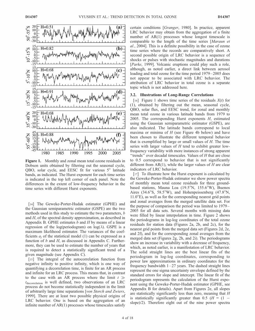
[16] Figure 1 shows time series of the residuals X(t) for(1), obtained by filtering out the mean, seasonal cycle,QBO, solar flux, and EESC trend, for zonal and monthlymean total ozone in various latitude bands from 1979 to2005. The corresponding Hurst exponents H, estimatedusing the Gaussian semiparametric estimator (GSPE), arealso indicated. The latitude bands correspond to localmaxima or minima of H (see Figure 4b below) and havebeen chosen to illustrate the different temporal behaviorthat is exemplified by large or small values of H. The timeseries with larger values of H tend to exhibit greater low-frequency variability with more instances of strong apparent‘‘trends’’ over decadal timescales. Values of H that are closeto 0.5 correspond to behavior that is not significantlydifferent from AR(1), while the larger values of H are clearindicators of LRC behavior.[17] To illustrate how the Hurst exponent is calculated by

the Geweke-Porter-Hudak estimator we show power spectraof monthly mean total ozone residuals for three ground-based stations, Mauna Loa (19.5�N, 155.6�W), BuenosAires (34.6�S, 58.5�W), and Hohenpeissenberg (47.8�N,11.0�E), as well as for the corresponding nearest grid pointsand zonal averages from the merged satellite data set. Forthe purpose of comparison the period was limited to 1979–2005 for all data sets. Several months with missing datawere filled by linear interpolation in time. Figure 2 showsthe periodograms in log-log coordinates of the total ozoneresiduals for station data (Figures 2a, 2b, and 2c), for thenearest grid points from the merged data set (Figures 2d, 2e,and 2f), and for the corresponding zonal averages from themerged data set (Figures 2g, 2h, and 2i). The periodogramsshow an increase in variability with a decrease of frequency,which, as noted earlier, is a manifestation of LRC behavior.The solid straight lines are the best linear fits of theperiodogram in log-log coordinates, corresponding topower law approximations in ordinary coordinates for thefrequency bandwidth 1–27 years. The dashed straight linesrepresent the one sigma uncertainty envelope defined by thestandard errors for slope and intercept. The linear fit of theperiodogram represents the calculation of the Hurst expo-nent using the Geweke-Porter-Hudak estimator (GPHE, seeAppendix B for details). Apart from Figures 2e, all slopesare statistically significantly less than zero, meaning that His statistically significantly greater than 0.5 (H = (1 �slope)/2). Therefore eight out of the nine power spectra

Figure 1. Monthly and zonal mean total ozone residuals inDobson units obtained by filtering out the seasonal cycle,QBO, solar cycle, and EESC fit for various 5� latitudebands, as indicated. The Hurst exponent for each time seriesis indicated in the top left corner of each panel. Note thedifferences in the extent of low-frequency behavior in thetime series with different Hurst exponents.


4 of 18

D14307

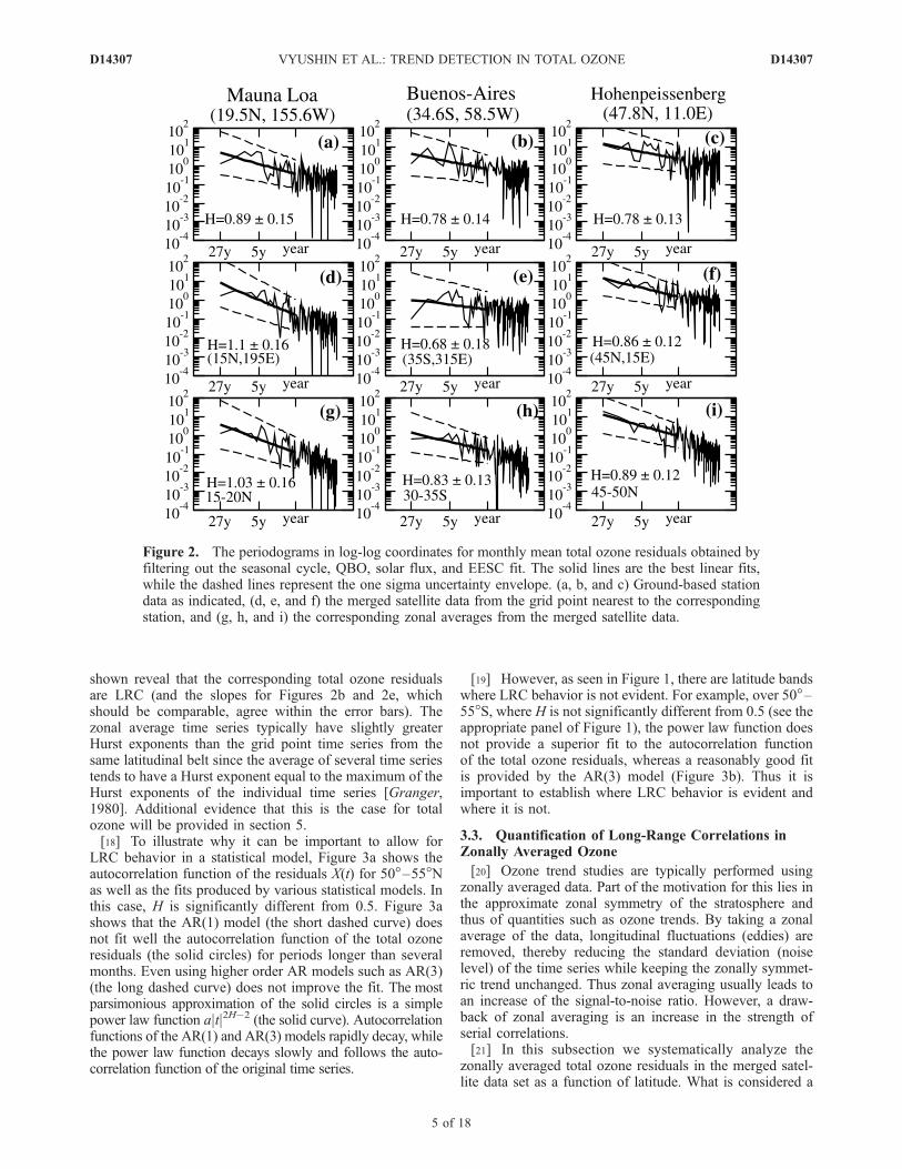
shown reveal that the corresponding total ozone residualsare LRC (and the slopes for Figures 2b and 2e, whichshould be comparable, agree within the error bars). Thezonal average time series typically have slightly greaterHurst exponents than the grid point time series from thesame latitudinal belt since the average of several time seriestends to have a Hurst exponent equal to the maximum of theHurst exponents of the individual time series [Granger,1980]. Additional evidence that this is the case for totalozone will be provided in section 5.[18] To illustrate why it can be important to allow for

LRC behavior in a statistical model, Figure 3a shows theautocorrelation function of the residuals X(t) for 50�–55�Nas well as the fits produced by various statistical models. Inthis case, H is significantly different from 0.5. Figure 3ashows that the AR(1) model (the short dashed curve) doesnot fit well the autocorrelation function of the total ozoneresiduals (the solid circles) for periods longer than severalmonths. Even using higher order AR models such as AR(3)(the long dashed curve) does not improve the fit. The mostparsimonious approximation of the solid circles is a simplepower law function ajtj2H�2 (the solid curve). Autocorrelationfunctions of the AR(1) and AR(3) models rapidly decay, whilethe power law function decays slowly and follows the auto-correlation function of the original time series.

[19] However, as seen in Figure 1, there are latitude bandswhere LRC behavior is not evident. For example, over 50�–55�S, where H is not significantly different from 0.5 (see theappropriate panel of Figure 1), the power law function doesnot provide a superior fit to the autocorrelation functionof the total ozone residuals, whereas a reasonably good fitis provided by the AR(3) model (Figure 3b). Thus it isimportant to establish where LRC behavior is evident andwhere it is not.

3.3. Quantification of Long-Range Correlations inZonally Averaged Ozone

[20] Ozone trend studies are typically performed usingzonally averaged data. Part of the motivation for this lies inthe approximate zonal symmetry of the stratosphere andthus of quantities such as ozone trends. By taking a zonalaverage of the data, longitudinal fluctuations (eddies) areremoved, thereby reducing the standard deviation (noiselevel) of the time series while keeping the zonally symmet-ric trend unchanged. Thus zonal averaging usually leads toan increase of the signal-to-noise ratio. However, a draw-back of zonal averaging is an increase in the strength ofserial correlations.[21] In this subsection we systematically analyze the

zonally averaged total ozone residuals in the merged satel-lite data set as a function of latitude. What is considered a

Figure 2. The periodograms in log-log coordinates for monthly mean total ozone residuals obtained byfiltering out the seasonal cycle, QBO, solar flux, and EESC fit. The solid lines are the best linear fits,while the dashed lines represent the one sigma uncertainty envelope. (a, b, and c) Ground-based stationdata as indicated, (d, e, and f) the merged satellite data from the grid point nearest to the correspondingstation, and (g, h, and i) the corresponding zonal averages from the merged satellite data.


5 of 18

D14307

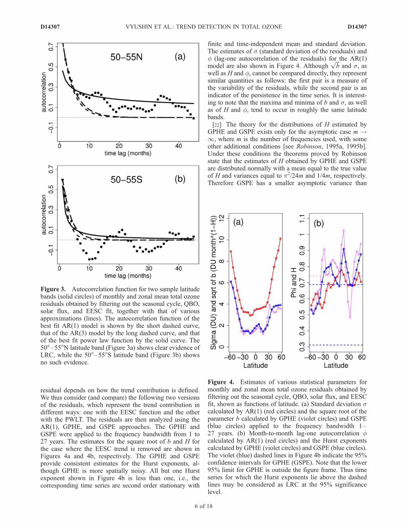
residual depends on how the trend contribution is defined.We thus consider (and compare) the following two versionsof the residuals, which represent the trend contribution indifferent ways: one with the EESC function and the otherwith the PWLT. The residuals are then analyzed using theAR(1), GPHE, and GSPE approaches. The GPHE andGSPE were applied to the frequency bandwidth from 1 to27 years. The estimates for the square root of b and H forthe case where the EESC trend is removed are shown inFigures 4a and 4b, respectively. The GPHE and GSPEprovide consistent estimates for the Hurst exponents, al-though GPHE is more spatially noisy. All but one Hurstexponent shown in Figure 4b is less than one, i.e., thecorresponding time series are second order stationary with

finite and time-independent mean and standard deviation.The estimates of s (standard deviation of the residuals) andf (lag-one autocorrelation of the residuals) for the AR(1)model are also shown in Figure 4. Although

ffiffiffib

pand s, as

well as H and f, cannot be compared directly, they representsimilar quantities as follows: the first pair is a measure ofthe variability of the residuals, while the second pair is anindicator of the persistence in the time series. It is interest-ing to note that the maxima and minima of b and s, as wellas of H and f, tend to occur in roughly the same latitudebands.[22] The theory for the distributions of H estimated by

GPHE and GSPE exists only for the asymptotic case m !1, where m is the number of frequencies used, with someother additional conditions [see Robinson, 1995a, 1995b].Under these conditions the theorems proved by Robinsonstate that the estimates of H obtained by GPHE and GSPEare distributed normally with a mean equal to the true valueof H and variances equal to p2/24m and 1/4m, respectively.Therefore GSPE has a smaller asymptotic variance than

Figure 3. Autocorrelation function for two sample latitudebands (solid circles) of monthly and zonal mean total ozoneresiduals obtained by filtering out the seasonal cycle, QBO,solar flux, and EESC fit, together with that of variousapproximations (lines). The autocorrelation function of thebest fit AR(1) model is shown by the short dashed curve,that of the AR(3) model by the long dashed curve, and thatof the best fit power law function by the solid curve. The50�–55�N latitude band (Figure 3a) shows clear evidence ofLRC, while the 50�–55�S latitude band (Figure 3b) showsno such evidence.

Figure 4. Estimates of various statistical parameters formonthly and zonal mean total ozone residuals obtained byfiltering out the seasonal cycle, QBO, solar flux, and EESCfit, shown as functions of latitude. (a) Standard deviation scalculated by AR(1) (red circles) and the square root of theparameter b calculated by GPHE (violet circles) and GSPE(blue circles) applied to the frequency bandwidth 1–27 years. (b) Month-to-month lag-one autocorrelation fcalculated by AR(1) (red circles) and the Hurst exponentscalculated by GPHE (violet circles) and GSPE (blue circles).The violet (blue) dashed lines in Figure 4b indicate the 95%confidence intervals for GPHE (GSPE). Note that the lower95% limit for GPHE is outside the figure frame. Thus timeseries for which the Hurst exponents lie above the dashedlines may be considered as LRC at the 95% significancelevel.


6 of 18

D14307

GPHE by a factor of p2/6. The values 0.5 ± 1.96 p/ffiffiffiffiffiffiffiffiffi24m

p

and 0.5 ± 1.96/(2ffiffiffiffim

p) are indicated in Figure 4b by dashed

violet and blue lines, respectively. All Hurst exponentestimates located above these lines may be considered asgreater than 0.5 with 95% statistical significance, meaningthat the corresponding time series may be parsimoniouslydescribed by an LRC model. This applies to just over halfthe latitudes analyzed. There is clear evidence of LRC atcertain latitude bands, while at other latitude bands theautocorrelation behavior is not significantly different fromthe AR model. Interestingly, the latitudinal structure of LRCbehavior is quite different in the two hemispheres.[23] It should be emphasized that the LRC methods

discussed here are based on asymptotic approximations atlow frequencies, and therefore they could be sensitive to thefrequency interval used for the parameter estimation asfollows: a wider interval may yield a bias in the estimates,while a narrower interval results in larger uncertainties ofthe estimates. Figure 5 is similar to Figure 4, except thatGPHE and GSPE were applied to the entire frequencybandwidth from 2 months to 27 years [The results for theAR(1) model (red circles) are identical to those shown inFigure 4]. The Hurst exponents shown in Figure 5b arealmost everywhere greater than one; that is, they belong toa nonstationary range. However, Figures 2g, 2h, and 2idemonstrate that the periodograms for the zonal averageshave steeper slopes for the bandwidth 2 months to 1 yearthan for the bandwidth 1–27 years. Therefore the factthat the calculated Hurst exponents are greater than one in

this case is an artifact of including the high-frequency(subannual) part of the spectrum in the fit.[24] To investigate the dependence of the residuals on the

definition of the long-term trend, the calculations wererepeated but with the residuals defined by using the PWLTin (1) instead of the EESC time series. The results areshown in Figure 6 and may be compared with Figure 4. Inthe Southern Hemisphere the statistical parameters (andtheir latitudinal variations) are very similar in the two cases.However, there is a distinct change in the Northern Hemi-sphere, where the Hurst exponents decrease by about 0.1.Over a broad region of the midlatitudes H is no longersignificantly different from 0.5, implying the loss of LRC inthis region, and at the highest subpolar latitudes, the extentof LRC behavior is strongly reduced. Inspecting Figure 1f,corresponding to 55�–60�N, it is evident that the major low-frequency variation in the residual defined relative to EESCprojects strongly on a piecewise-linear trend with a turningpoint in early 1996, and its contribution to the residual istherefore substantially reduced when the PWLT function isused to define the long-term trend. This is illustrated byFigure 7, which shows the ozone time series for 55�–60�N(with mean, solar, QBO, and seasonal cycle filtered out)together with the EESC and PWLT fits (Figure 7a) and thePWLT residual (Figure 7b); the latter may be compared withthe EESC residual shown in Figure 1f.

4. Significance of Long-Term Trends inZonal-Mean Total Ozone

4.1. Long-Term Ozone Decline

[25] The statistical model used to describe the noise doesnot affect the mean trend estimated by equation (1), but it

Figure 5. Same as Figure 4, but with GPHE and GSPEapplied to the frequency bandwidth 2 months to 27 years.Note the different vertical scale in Figure 5b compared withFigure 4b. This analysis yields spurious results, namely,Hurst exponents greater than unity (indicating nonstationarybehavior). The figure is included to highlight the importanceof choosing an appropriate bandwidth (see text for furtherdiscussion).

Figure 6. Same as Figure 4, but with PWLT filtered outinstead of EESC to describe the long-term trend. The Hurstexponents are similar to those in Figure 4 in the SouthernHemisphere, but are reduced in magnitude by about 0.1 inthe Northern Hemisphere.


7 of 18

D14307

does affect the estimated uncertainty of the trend. Theregression coefficient of the total ozone anomalies on theEESC time series is shown in Figure 8a as a function oflatitude for the period 1979–2005. The magnitude of theregression coefficient basically displays the sensitivity oftotal ozone in that latitude band to the stratospheric abun-dance of ozone-depleting substances as represented by theEESC. For comparison with other estimates the result ispresented in Dobson units per year for the time period1979–1995, during which the EESC time series is nearlylinear with a net change of approximately 1.6 ppb ofchlorine. As is well known, the long-term ozone declinehas a minimum in the tropics and increases toward the poles,with larger values in the Southern Hemisphere as comparedwith the Northern Hemisphere midlatitudes. The strongincrease of the Southern Hemisphere trend with latitude isindicative of the large influence of Antarctic ozone loss on theSouthern Hemisphere midlatitude long-term decline [e.g.,Chipperfield, 2003, Fioletov and Shepherd, 2005].[26] The error bars in Figure 8a indicate the 95% confi-

dence intervals estimated under AR(1) and LRC hypothesesconcerning autocorrelation of the residuals. The trend uncer-tainties under the LRC hypothesis are evidently wider thanthose under the AR(1) hypothesis. The differences are partic-ularly large where H exceeds 0.7, which, from Figure 4b,occurs basically everywhere north of 35�S. In this regionthe standard deviation of the trend under the LRC hypoth-esis is up to 1.5 times larger than that under the AR(1)hypothesis. This broadens the range of tropical latitudesover which the trend is not significant at the 95% level andsubstantially increases the already large trend uncertainty innorthern middle and high latitudes. In contrast, the Hurstexponent is about 0.5–0.6 over the southern middle andhigh latitudes, i.e., the residuals have relatively weak long-

range correlations, and in this region, the trend uncertaintiesestimated under the LRC and AR(1) hypotheses are nearlyidentical.[27] Figure 8b shows the corresponding results for the

linear trend from 1979 to 1995 (the declining part of thePWLT function). The means and standard deviations [inclu-ding the differences between the latter for LRC and AR(1)hypotheses for the residuals] are very similar to thoseobtained using the EESC fit in Figure 8a, except in northernmiddle and high latitudes where the PWLT-derived trend islarger. This is consistent with the behavior already noted insection 3.3, where the strong decline in total ozone innorthern middle and high latitudes in the early 1990s andits subsequent increase in the late 1990s is interpreted asLRC noise relative to the EESC time series, but contributesto the long-term decline (with weaker LRC behavior in thenoise) under PWLT.

4.2. Recent and Future Ozone Increase

[28] The EESC time series can be well approximatedby two linear functions, with the first slope equal to about1 ppb/decade for the period before the EESC maximum inthe second half of the 1990s and the second slope equal toabout �0.34 ppb/decade for the period after the EESCmaximum.[29] Therefore it is possible to estimate the expected rate

of ozone increase after the late 1990s from the EESC fit: Itis just the regression coefficient plotted in Figure 8amultiplied by �0.34. The result is shown in Figure 9 bythe dotted-dashed curve. For comparison, the positive trendestimated from PWLT, which is the observed linear trendover the time period 1996–2005, is shown by the diamondsconnected by the solid curve together with its uncertaintiesunder both the AR(1) and LRC hypotheses. The two trends

Figure 7. (a) Monthly and zonal mean total ozone anomalies for the 55�–60�N latitude band obtainedby filtering out the seasonal cycle, QBO, and solar flux, together with the EESC (solid) and PWLT(dashed) fits. (b) The corresponding total ozone residuals when the PWLT fit is removed. Figure 7b maybe compared directly with the EESC-based residuals shown in Figure 1f.


8 of 18

D14307

are fairly similar in southern middle and high latitudes,although the uncertainties on the observed trends encom-pass zero. In northern middle and high latitudes, however,the observed linear trend is roughly four times the EESC-predicted trend and is actually statistically significant over40�–50�N according to the PWLT estimate of the noise.Thus, once again in northern middle and high latitudes, wehave a major difference between the analysis provided bythe EESC- and PWLT-based models, although this differ-ence is within the 95% error bars.[30] Once the analytical relation between the trend uncer-

tainty and the length of the time series is known, it ispossible to calculate the number of years required to detect acertain trend with a given error and its dependence onlocation. This is important from a practical point of viewfor designing an ozone-monitoring strategy. The number ofyears required to detect future ozone trends was studied byWeatherhead et al. [2000] using the AR(1) model. Here weexpand on Weatherhead et al.’s results by including anallowance for LRC behavior. The methods and formulasused here to calculate the number of years are described inAppendix C.[31] We first consider the number of years required to

detect a trend of a given magnitude, without reference to themagnitude of the expected trend. With the noise estimated

relative to the EESC trend function (as in Figure 4), thenumber of years required to detect a 1 DU/year trend inzonal mean total ozone at the 95% significance level underthe AR(1) and the LRC hypotheses is shown in Figure 10a.The latitudinal structure primarily reflects that of the vari-ability (cf. Figure 4a), with the shortest number of yearsbeing required in the tropics (30�S–30�N). However, theimpact of long-term memory (cf. Figure 4b) mainlyaccounts for the hemispheric asymmetry in Figure 10a,increasing the number of years required in northern ascompared with southern latitudes. In those latitude bandsfor which the Hurst exponents are below 0.7, both theAR(1) and LRC models give consistent estimates of thenumber of years required, whereas, in other latitude bands,and especially in northern subtropical and high-subpolarlatitudes, LRC behavior considerably lengthens the timerequired to detect a given trend by a factor of up to 1.5 or so.[32] If the noise is estimated according to the PWLT trend

function (as in Figure 6), then the number of years requiredto detect a 1 DU/year trend is virtually identical to thatshown in Figure 10a in the Southern Hemisphere, but is, asexpected, reduced and closer to that estimated from theAR(1) model in the Northern Hemisphere (not shown).Figure 10b shows the same estimates as in Figure 10a,except that, in estimating the statistical parameters b and Hunder the LRC hypothesis, GPHE and GSPE were appliedto the frequency bandwidth from 2 months to 27 years (cf.Figure 5). The number of years in this case is severaltimes larger than for the proper bandwidth (1–27 years).We include Figure 10b here to emphasize the importance

Figure 8. (a) Regression coefficients of monthly and zonalmean total ozone anomalies (obtained by filtering out theseasonal cycle, QBO, and solar flux) on EESC for theperiod 1979–2005. (b) The first (declining) slope ofthe PWLT fit for the period 1979–1995. The regressioncoefficients in Figure 8a are scaled so as to be comparable tothe linear trend over 1979–1995; thus the two panelsrepresent, respectively, the EESC-based and PWLT-basedestimates of the long-term ozone decline. The 95%confidence intervals shown are calculated under the follow-ing two alternative assumptions: AR(1) (light grey region)and LRC (dark grey region). Details of the confidence-interval calculations can be found in Appendix C.

Figure 9. The EESC-based linear trend calculated for thedeclining part of EESC (solid circles connected by thedashed line) is compared to the second (increasing) slope ofthe PWLT fit for the period 1996–2005 (diamondsconnected by the solid line), the latter with 95% confidenceintervals calculated under the AR(1) (light grey region) andLRC assumptions (dark grey region).


9 of 18

D14307

of a correct bandwidth choice for Hurst exponent estima-tion under the LRC model.[33] We now consider the latitudinal dependence of the

expected trends, and estimate the number of years requiredto detect a statistically significant ozone increase if thepositive trends are those estimated in Figure 9 accordingto either the EESC or PWLT models. In both cases the‘‘detection’’ is made here under the assumption that thetrend is independent of the past trend (prior to 2000 forEESC, prior to 1996 for PWLT), and both AR(1) and LRCestimates are computed. Consider first the detection of thepositive ozone trend expected from the EESC decline,shown in Figure 11a. As was noted by Weatherhead et al.[2000], southern middle and high latitudes are the bestplaces to detect ozone recovery according to the AR(1)model; the same is seen to be true for the LRC model. In theNorthern Hemisphere, there appears to be an optimal regionfor detection of ozone recovery around 30�–40�N; on eitherside, there is a strong effect of LRC behavior on the numberof years required, especially at northern middle and highlatitudes where, according to the LRC model, it should takeabout 1.5 times longer to detect the expected trends thanestimated under the AR(1) model.

[34] The number of years required to detect the observedtrend from 1996 to 2005 at the 95% significance level,according to the PWLT analysis, is shown in Figure 11b.The length of the observed record (10 years) is indicated bythe dotted line; at latitudes with points lying below this line,a significant trend has therefore already been detected(cf. Figure 9). The result is completely different fromFigure 11a. According to the PWLT analysis, the bestplace to detect ozone recovery is northern middle and highlatitudes (moreover, in this region, a positive trend is eitheron the verge of being detected or has already beendetected) and the second best region is in the equatorialzone. However, at southern high latitudes, the number ofyears required, �18, is similar between the EESC andPWLT analyses and is well estimated by the AR(1) modelin both cases. This is expected given the consistency atthese latitudes of the EESC-predicted and observed recenttrends, the consistency of the EESC- and PWLT-derivednoise estimates, and the absence of LRC.

5. Longitudinal Structure

[35] In this section we present the latitude-longitudedistributions of some of the statistical parameters discussedabove for zonal averages. Figures 12a and 12b show thespatial distributions of the AR(1) month-to-month autocor-relation parameter f and the Hurst exponent H, respectively,

Figure 10. (a) The number of years required to detect a1 DU/year trend at the 95% significance level under theAR(1) (red curve) and LRC assumptions (violet curveshows GPHE, blue curve shows GSPE) applied to thefrequency bandwidth 1–27 years of the monthly mean totalozone residuals obtained by filtering out the seasonal cycle,QBO, solar flux, and EESC fit. (b) The same as Figure 10a,but using the frequency bandwidth 2 months to 27 years forthe LRC estimates (the red curve is the same in bothpanels). Note the different vertical scales in the two panels.Figure 10b is a spurious result (cf. Figure 5) and is shown tohighlight the importance of choosing an appropriatebandwidth for the analysis.

Figure 11. (a) The number of years since 2000 required todetect the EESC-based linear trend calculated for thedeclining part of EESC at the 95% significance level underthe following two alternative assumptions: AR(1) (redcurve) and LRC (blue curve, based on GSPE). (b) The sameas Figure 11a, but for the PWLT-based trend calculated forthe period 1996–2005, so the value represents the numberof years after 1996. Values higher than 100 years are plottedas 100 years. Note the similarity of the two estimates insouthern middle and high latitudes, but the large differencesin the Northern Hemisphere. See text for details.


10 of 18

D14307

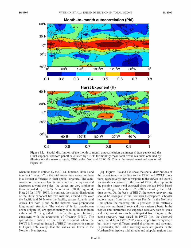
when the trend is defined by the EESC function. Both f andH reflect ‘‘memory’’ in the total ozone time series but thereis a distinct difference in their spatial structure. The auto-correlation parameter has its maximum at the equator anddecreases toward the poles; the values are very similar tothose reported by Weatherhead et al. [2000, Figure 4,Plate 3] for 1979–1998. In contrast, the spatial distributionof the Hurst exponent has two maxima, around 15�S overthe Pacific and 20�N over the Pacific, eastern Atlantic, andAfrica. For both f and H, the maxima have pronouncedlongitudinal structure. The values of H for zonal-meanozone (Figure 4b) are approximately equal to the maximumvalues of H for gridded ozone at the given latitude,consistent with the arguments of Granger [1980]. Thespatial distribution of the Hurst exponent when thePWLT is filtered out instead of EESC (not shown) is similarto Figure 12b, except that the values are lower in theNorthern Hemisphere.

[36] Figures 13a and 13b show the spatial distributions ofthe recent trends according to the EESC and PWLT func-tions, respectively; they correspond to the curves in Figure 9for zonal-mean ozone. In the case of EESC, this representsthe positive linear trend expected since the late 1990s basedon the fitting of the entire 1979–2005 record by the EESCtime series. On the basis of EESC, the ozone recovery rateshould be strongest in the Southern Hemisphere subpolarregions, apart from the south-west Pacific. In the NorthernHemisphere the recovery rate is predicted to be relativelystrong over northern Europe and over eastern Siberia. In thetropics and subtropics the expected recovery rate is weakand very zonal. As can be anticipated from Figure 9, theozone recovery rates based on PWLT (i.e., the observedlinear trend from 1996–2005) are also positive everywherebut have a very different spatial distribution and strength.In particular, the PWLT recovery rates are greater in theNorthern Hemisphere midlatitudes and subpolar regions than

Figure 12. Spatial distribution of the month-to-month autocorrelation parameter f (top panel) and theHurst exponent (bottom panel) calculated by GSPE for monthly mean total ozone residuals obtained byfiltering out the seasonal cycle, QBO, solar flux, and EESC fit. This is the two-dimensional version ofFigure 4b.


11 of 18

D14307

in the Southern Hemisphere; the trends are especially strongover Siberia, the North Pacific, the northern midlatitudeAtlantic, and Europe. The only place in the Northern Hemi-sphere midlatitudes and subpolar regions where the trends arerelatively weak is the subpolar North Atlantic. The spatialdistribution of the recent PWLT over the southern ocean isopposite to that for the EESC trend, with a maximum ratherthan a minimum over the south-west Pacific.[37] Finally, Figure 14 presents the number of years from

the year 2000 required to detect the expected EESC-basedozone trends shown in Figure 13a, based on the LRC noiseestimates computed from the entire time series (with the EESCtrend filtered out). The Figure allows us to identify the optimallocations to make long-term ground-based total ozone obser-vations. For example, it would be desirable to have somestations in the southern subpolar Atlantic since the number ofyears required to detect ozone recovery has a minimum in thatregion, where it varies between 12 and 20 years. In the

Northern Hemisphere the minimum is located in the zonalband around 35�N and varies between 20 and 30 years.

6. Summary and Discussion

[38] The statistical analysis of long-term changes in totalozone has traditionally been performed assuming that theresiduals, which represent the noise in the system, are welldescribed by an AR(1) model. In this study the total ozonerecord from 1979 to 2005 has been examined for theexistence of long-range correlations (LRC), implying adeviation from AR(1) behavior with an unbounded decor-relation time. The existence of LRC behavior in total ozonewould reduce the statistical significance of a given trend,and lengthen the number of years required to detect a trend,from that estimated using an AR(1) model. We employ themerged satellite data set prepared by NASA which com-bines version 8 of TOMS and SBUV total ozone data [Frithet al., 2004; Stolarski and Frith, 2006], use well-basedspectral estimation techniques to quantify LRC paying

Figure 13. Spatial distribution of the EESC-based linear trend calculated for the declining part of EESCin DU/year (top panel) and the second (increasing) slope of the PWLT fit for the period 1996–2005(bottom panel). This is the two-dimensional version of Figure 9.


12 of 18

D14307

proper attention to the frequency bandwidth, and filter long-term time periodic signals (QBO, solar) which can givespurious indications of LRC behavior. The analysis mainlyconcerns zonal-mean ozone, although some station data andgridded satellite data are also considered. However, theanalysis is restricted to 60�S–60�N, as, in polar regions,the satellite data have gaps during polar night.[39] We first summarize the results obtained when the

long-term total ozone changes are represented in terms ofthe EESC time series. Clear evidence of LRC is foundbasically everywhere north of 35�S. In the southern middleand high latitudes the correlation behavior is not signifi-cantly different (at the 95% significance level) from that ofthe AR(1) model. In the regions with strong LRC behavior,uncertainties in the magnitude of the long-term ozonedecline attributable to EESC are increased by about a factorof 1.5 compared with those estimated from AR(1); thisincludes the northern middle and high latitudes, where theAR(1)-based uncertainties are already quite large. However,the strongest long-term ozone decline is found at thesouthern middle and high latitudes, and there, the AR(1)estimates are found to be reliable.[40] Analogous results are found for the number of years

(from 2000) required to detect the increase of ozoneexpected from the anticipated decline of EESC. We confirmWeatherhead et al.’s [2000] finding, on the basis of theAR(1) model, that southern middle and high latitudesshould be the optimal place (within the 60�S–60�N region)to detect ozone increase; at these latitudes, we have thecombination of the strongest expected trend, the apparentabsence of LRC behavior, and the shortest autocorrelationtimes. The required detection time (to 95% significance) isabout 18 years for zonal-mean ozone at 60�S, but is even afew years shorter in the subpolar South Atlantic. Whilelimited regions have higher noise levels, they also haveweaker serial correlations. The recent observed behavior oftotal ozone in these regions is consistent with the EESC-predicted trend, but detection of an ozone increase attributableto EESC is not expected until sometime late in the decade

2010–2020. In the Northern Hemisphere, detection of ozoneincrease is more challenging. There appears to be a narrowband around 35�N where LRC behavior is relatively weak andthe required number of years is around 30, but in northernmiddle and high latitudes, the required number of years isincreased from around 25–35 to around 30–60 by LRC.[41] Although the representation of long-term ozone

changes in terms of the EESC time series is preferred, giventhe a priori nature of the representation, a commonly usedalternative is a piecewise-linear trend (PWLT) with aturning point in the second half of the 1990s. Thereforewe compared the results obtained using the two differentrepresentations of the long-term changes. In our implemen-tation of PWLT we use a turning point in early 1996.The estimates of the noise and the long-term ozone declineare essentially the same for the two cases in the SouthernHemisphere, but there is a notable discrepancy in theNorthern Hemisphere (particularly at northern middle andhigh latitudes) where the strong decrease in ozone in theearly 1990s, and its subsequent increase in the late 1990s,are interpreted mainly as LRC noise relative to EESC, butproject strongly on the long-term changes (thereby reducingthe strength of the LRC behavior) relative to the PWLT.This difference affects all subsequent estimates. For exam-ple, according to PWLT, the long-term ozone decline innorthern middle and high (subpolar) latitudes is comparablein magnitude to that in the Southern Hemisphere; the recentozone increase (since 1996) is strongest in this region, andmarginally statistically significant (at the 95% significancelevel) indicating that a positive ozone trend is already on theverge of being detected.[42] The natural question is, then, which representation of

the long-term changes (and thus of the noise) is correct? Wedo not attempt to answer this question definitively, but a fewcomments may be in order. If one adopts the EESCperspective, then the results seem physically sensible asfollows: we know that the annual-mean long-term ozonedecline, from pre-1980 levels to those characteristic of the2000 time period, over the middle and high (subpolar)

Figure 14. The number of years since 2000 required to detect the EESC-based linear trend calculatedfor the declining part of EESC at the 95% significance level under the LRC assumption (based on GSPE).This is the two-dimensional version of Figure 11a.


13 of 18

D14307

latitudes has been much greater in the Southern Hemisphereas compared with the Northern Hemisphere, roughly 6% ascompared with 3% [WMO, 2003]. Furthermore, we knowthat the Northern Hemisphere ozone exhibits more interan-nual variability than the Southern Hemisphere ozone be-cause of the greater stratospheric dynamical variability inthe Northern Hemisphere, which is for well-understoodreasons. What remains then to be understood is the physicalorigin of the LRC, especially in northern middle and highlatitudes. If it is the existence of AR timescales comparableto the 27-year observational record, then are these time-scales associated with natural variability or with climatechange? These questions can likely only be answered withclimate models.[43] If, on the other hand, one adopts the PWLT perspec-

tive, then one is forced to consider the strong decline ofnorthern middle and high latitude ozone in the early 1990s,and its subsequent increase in the late 1990s, as part of thesignal and account for it. One possibility often considered[e.g., Solomon et al., 1996] is that the increased strato-spheric aerosol from the Mount Pinatubo volcanic eruptionin 1991 amplified the EESC-associated ozone loss. Theproblem with this argument is that there was no corres-ponding ozone decrease observed in the Southern Hemi-sphere, even though EESC and aerosol abundances werecomparable [Bodeker et al., 2001]. Another argument is thatthe behavior reflects decadal-scale variations in strato-spheric wave forcing [e.g.,Randel et al., 2002;Hadjinicolaouet al., 2005], which would affect ozone both through changesin transport and changes in chemical ozone loss, especially inthe Arctic which would then affect the annual mean subpolarozone abundances through the transport of ozone-depletedair. The impact of long-term changes in stratospheric waveforcing on both polar and midlatitude ozone is well estab-lished [WMO, 2003]. However, attributing the ozone changesto changes in wave forcing merely changes the problem tothat of accounting for the variations in wave forcing. Inprinciple, they could be part of the signal or part of the noise.Yet the use of PWLT involves the implicit assumption that therecent strong positive trend in northern middle- and high-latitude ozone is secular and can be extrapolated; moreover,by regarding this trend as part of the signal rather than part ofthe noise, the estimated noise is reduced and the LRCbehavior weakened, and the estimated significance of thetrend thereby increased. So far, no mechanism that could givesuch a statistically significant positive trend in the northernmiddle and high latitude ozone has been put forward.

Appendix A: Introduction to Long-RangeCorrelated Processes

[44] Development of the theory for a class of stochasticprocesses with long-range correlated increments was origina-ted by Kolmogorov in two short notes [Kolmogorov, 1940a,1940b] during his studies of turbulence. The seminal paper ofMandelbrot and Van Ness [1968] developed many of itsproperties and named it by the class of self-similar processes.[45] A real-valued stochastic process Z={Z(t)} t2R is self-

similar with index H > 0 if, for any a > 0,

Z atð Þf gt2R ¼d aHZðtÞ� �

t2R; ðA1Þ

where ¼d denotes the equality of the finite-dimensionaldistributions [Taqqu, 2002]. In this article we use incre-ments of a self-similar process for modeling residuals of thetotal ozone time series. The autocovariance of the incrementsequence Xi = Zi � Zi�1 of a self-similar process

g tð Þ ¼ cov Xi;Xiþtð Þ ¼ s2

2jt þ 1j2H � 2jtj2H þ jt � 1j2Hh i

asymptotically decays by a power law [e.g., Beran, 1994]

g tð Þ � s 2H 2H � 1ð Þjtj2H�2; as t ! 1: ðA2Þ

[46] The increments of a self-similar stochastic processfor 1/2 < H < 1 have long-range correlated behavior, sinceg(t) decays to zero so slowly that

P1t¼�1 g tð Þ diverges.

There are no long-range correlations in the ‘‘blue’’ noisecase (H < 0.5). Usually for climatic time series 0.5 � H <1.0. The case H = 0.5 corresponds to short-memory pro-cesses, which can be well modeled by conventional auto-regressive moving average (ARMA) models. Spectraldensity of the increment sequence of a self-similar processscales by a power law in the vicinity of the origin

fX lð Þ ¼ bjlj1�2H ; as l ! 0: ðA3Þ

[47] The next appendix provides an overview of spectralstatistical methods for estimating parameters b and H of agiven time series.

Appendix B: Statistical Methods for Estimationof b and H

[48] In the beginning of the estimation process, one calcu-lates the discrete Fourier transform of a given time series

w jð Þ ¼ 1ffiffiffiffiffiffiffiffi2pn

pXnt¼1

X tð Þeit2p j

n ; j ¼ 1:: n=2½ �; ðB1Þ

where square brackets denote rounding toward zero, and theperiodogram—an estimate of the spectral density

I jð Þ ¼ w jð Þj j2¼ 1

2pn

Xnt¼1

X tð Þe it2pjn

2

; ðB2Þ

where n is the time series length. The goal is to approximatethe estimate of the spectral density I(j) by an analytical formfor the spectral density, in our case f (b, H, l) = bjlj1 � 2H,where l = 2pj/n. There are several semiparametric methodsfor estimating b and H. For a recent review, see for instanceMoulines and Soulier [2002]. Many of them might bedescribed in terms of the so-called contrast function k (u, v),which can be thought of as a distance between functions uand v. Then the approximation process reduces to mini-mization of the following functional

K b;Hð Þ ¼ 1

m

Xmj¼1

k IðjÞ; f b;H ;2pjn

� �; ðB3Þ

where 1 < m � [n/2] is an index of the highest frequencyused. The meaning of the free parameter m is similar to the


14 of 18

D14307

order of autoregressive fractionally integrated movingaverage (ARFIMA) model. However, in contrast to theorder of ARFIMA, m has a clear physical sense. Forinstance, in our study, we focus mainly on interannualvariability of the monthly resolved total ozone and thuschoose m = n/12. In sections 3.3 and 4.2, we comparedsome results for m = n/2 (full spectrum) and m = n/12. Inthis article we apply the following two methods ofsemiparametric estimation: Geweke-Porter-Hudak estimator(GPHE) and Gaussian semiparametric estimator (GSPE).GPHE was originally proposed by Geweke and Porter-Hudak [1983] and probably is the most popular, because ofits simple realization, semiparametric estimator used inapplications. GPHE corresponds to the contrast functionk(u, v) = (log(u) � log(v))2. Therefore it simply performs alog linear regression of the periodogram. For GPHEparameters b and H, which minimize K(b, H), can befound in a closed form. The graphical illustration of GPHEis shown in Figure 2. A more advanced estimator, GSPE,was introduced by Fox and Taqqu [1988]. Its contrastfunction is k(u, v) = log(u) + u/v. GSPE is a maximumlikelihood estimator. For GSPE the problem of minimiza-tion of K(b, H) can be reduced to a one-dimensionalminimization problem and solved using standard optimiza-tion technique. Rigorous mathematical justification of GPHEand GSPE was given by Robinson [1995a, 1995b],respectively. Robinson showed that GSPE is superior toGPHE. For instance, it has by a factor of p2/6 smallerasymptotic variance. In practice, we find that GSPE gives lessnoisy (spatially) and more robust estimates than GPHE.

Appendix C: Trend Variance and the Numberof Years Required to Detect a Trend

[49] For the purpose of trend analysis, memory is anissue. It is hard to distinguish a trend from natural variabilityin case time series is strongly serially correlated. Theimportance of taking into account LRC in trend analysiswas first realized by Bloomfield [1992] during his studies oftrends in surface air temperature. He proposed to useautoregressive fractionally integrated moving average(ARFIMA) model, introduced independently by Grangerand Joyeux [1980] and Hosking [1981], for modelingtemperature residuals. The idea is to fit the residuals,obtained after filtering out deterministic components of tem-perature time series such as seasonal cycle and trend, byARFIMA and, knowing analytical expression for the vari-ance of ARFIMA, calculate the variance of the trend.Bloomfield’s approach can be classified as sequential fullparametric estimation, since one first estimates and filters outthe trend and then estimates the parameters of ARFIMA.Joint full parametric estimation, when the trend and theparameters of ARFIMA are estimated simultaneously, wastheoretically justified by Robinson [2005] and was appliedto Northern Hemisphere SAT anomalies by Gil-Alana[2005]. The disadvantage of full parametric approach fortrend detection studies is a problem of choosing the correctorder of the ARFIMA, which itself is an issue [Beran et al.,1998]. An appealing way to overcome the issue of modelselection was proposed by Smith [1993]. He showed that it isimportant to fit only the low-frequency part of the residuals’spectrum using an asymptotic form of LRC spectral density

f (l) = bjlj1 � 2H with only two unknown parameters. Thenthe variance of the trend can be calculated on the basis ofthese two parameters. We follow this direction in our paper.This approach is classified as semiparametric since itrequires estimation only of a part of the whole parameterset. Smith and Chen [1996] advocated for joint estimation ofthe trend and the parameters b and H. Unfortunately, thistheoretically more correct approach is still missing a solidmathematical foundation. Therefore, in our article, we im-plement sequential semiparametric estimation; that is, wefirst estimate and filter out the trend from the time series andthen find b and H for the residuals using semiparametricestimation. The general theoretical justification of this meth-od is given by Yajima [1988].

C1. Estimation of Trend VarianceThrough Autocovariance

[50] Let’s consider a general linear estimator

x ¼Xnt¼1

l tð ÞY tð Þ: ðC1Þ

Variance of x may be expressed through autocovariance g ofY(t)

s 2 x�

¼Xnt¼1

Xns¼1

l tð Þl sð Þg t � sð Þ: ðC2Þ

For example, for the statistical model

Y tð Þ ¼ aþ by tð Þ þ X tð Þ; ðC3Þ

where y(t) is a certain explanatory variable (covariate) withzero mean and X(t) is a noise, the slope estimator b and itsvariance s2(b) may be written as follows

b ¼

Xn

t¼1y tð ÞY tð ÞXn

t¼1y2 tð Þ

; ðC4Þ

s2 b�

¼g 0ð Þ

Xn

t¼1y2 tð Þ þ 2

Xn�1

k¼1g kð Þ

Xn�k

j¼1y jð Þy jþ kð ÞXn

t¼1y2 tð Þ

� 2;

ðC5Þ

where n is the time series length; g(t) is the residuals’autocovariance function.

C2. Approximation of Autocovariance byExponential Function

[51] The most conventional way to proceed from thispoint is to use an exponential approximation for the resid-uals’ autocovariance function g(t) for deriving an asymp-totic formula for s(b). In principle, one can use the estimateof g(t) to numerically evaluate s(b). However, becauseof poor sampling properties of autocovariance functionestimates, statisticians prefer to use a certain approximation


15 of 18

D14307

of sample autocovariance function. To obtain an expo-nential approximation for the autocovariance function,one can fit an autoregressive model of the first order[AR(1)] to the noise. Symbolically, AR(1) can be writtenas follows:

X tð Þ ¼ fX t � 1ð Þ þ e tð Þ; ðC6Þ

where �1 < f < 1 is month-to-month autocorrelation(lag-one autocorrelation coefficient) and e(t) is a Gaussianwhite noise. Let’s review some of the AR(1) modelproperties. Autocovariance function of AR(1) decaysexponentially

gAR1ðtÞ ¼ s 2Xf

jtj: ðC7Þ

Spectral density of AR(1)

fAR1 lð Þ ¼ s 2X

2p1� f2

j1� fe�ilj2! s2

X

2p1þ f1� f

; as l ! 0;

where sX is the standard deviation of X(t).[52] In case we assume an AR(1) model for the monthly

resolved residuals X(t) and take y(t) = t � (n + 1)/2, wehave

sAR1 wð Þ � sX

N 3=2

ffiffiffiffiffiffiffiffiffiffiffiffi1þ f1� f

s; ðC8Þ

where w ¼ 12b is the estimate of the linear trend in unit y(t)per year; N is the length of a considered period in years[Weatherhead et al., 1998].

C3. Approximation of Autocovariance by Power LawFunction

[53] The alternative approach is to use a power lawapproximation of the sample autocovariance function whosecoefficients can be obtained by various estimation methods(see Appendix B). Substituting g(0) = sX

2, g(t) = at2H�2 for t> 0, and y(t) = t � (n + 1)/2 into equation (C5) andperforming asymptotic derivations we obtain

s 2 b�

� 36a 1� Hð ÞH 1þ Hð Þ 2H � 1ð Þ n

2H�4: ðC9Þ

Scaling factors of the autocovariance and the spectraldensity, a and b, are related as follows [e.g., Smith, 1993]:

a ¼ pbG 2H � 1ð Þ sin pHð Þ : ðC10Þ

Using this relation and some properties of the gammafunction we can rewrite the asymptotic formula for sðbÞ interms of b and H

sLRC b�

� B b;Hð ÞnH�2; ðC11Þ

where sLRC(b) is the standard deviation of the estimatedtrend under the LRC hypothesis and

B b;Hð Þ ¼

ffiffiffiffiffiffiffiffiffiffiffiffiffiffiffiffiffiffiffiffiffiffiffiffiffiffiffiffiffiffiffiffiffiffiffiffiffiffiffiffiffiffiffiffiffiffiffiffiffiffiffiffiffiffi72bp 1� Hð Þ

1þ Hð ÞG 2H þ 1ð Þ sin pHð Þ

s: ðC12Þ

Equations (C8) and (C11) were used in Figures 8b and 9.

C4. Estimation of Trend Variance ThroughSpectral Density

[54] Asymptotic formulas can be derived only in caseswhen the explanatory variable y(t) has a relatively simpleform such as a linear trend. In other cases, one can estimatethe standard deviation of a slope only numerically. From thenumerical point of view, it is more convenient to express theautocovariance through the spectral density. Thus replacingin formula (C2) the autocovariance by its expressionthrough the spectral density of X(t)

g kð Þ ¼Z p

�pe ilk f lð Þdl; ðC13Þ

we obtain

s 2 x�

¼Z p

�pU lð Þ f lð Þdl; ðC14Þ

where

U lð Þ ¼Xnt¼1

l tð Þe ilt

2

: ðC15Þ

The important thing is that almost all weight of the functionU(l) is concentrated near the origin. Therefore, for thecalculation of the trend uncertainty, the high-frequency partof the spectrum is not important. This fact motivates theimplementation of semiparametric (local) instead of fullparametric (global) statistical models [Smith, 1993].For example, in order to calculate the slope uncertainty incase y(t) = EESC(t) � EESCðtÞ, where EESC(t) is theequivalent effective stratospheric chlorine time series, andf (l) = bjlj1 � 2H, we used the following formula:

s 2 bEESC

� ¼ b

Z p=12

�p=12UEESC lð Þjlj1�2H

dl; ðC16Þ

where

UEESC lð Þ ¼Xnt¼1

EESC tð Þ � EESC tð ÞXn

s¼1EESC sð Þ � EESC sð Þ

� 2e ilt

2

:

Therefore we could neglect intra-annual variability [fre-quency ranges (�p/2, �p/12) and (p/12, p/2)] of the totalozone anomalies. Equation (C16) was used in Figure 8a.


16 of 18

D14307

C5. Estimation of the Number of Years Required toDetect a Trend

[55] The number of years required to detect a trend ofspecified magnitude jwj under the hypothesis that X(t) canbe well described by an AR(1) model according toWeatherhead et al. [1998] is as follows

N*AR1 �

2þ zp� �

sX

jwj

ffiffiffiffiffiffiffiffiffiffiffiffi1þ f1� f

s" #2=3

; ðC17Þ

where N*AR1 is the number of years required to detect a trend

of specified magnitude jwj (in particular, one may choosew ¼ w) and zp is the p percentile of the standard normaldistribution.[56] In this setup the probability to reject the test hypoth-

esis of zero trend when it is true is equal to 5% and theprobability to accept the hypothesis of zero trend when it isfalse is equal to p. The number of years required to detect alinear trend of specified magnitude jwj depends on three keyparameters in the AR(1) case (w, s, f).[57] From (C11) we derive an analogous equation for the

case when X(t) are long-range correlated

n*LRC �2þ zp� �

B b;Hð Þjbj

� � 12�H

: ðC18Þ

In the above equation, n is expressed in basic time units oftime series, i.e., days or months, and b has a unit y(t) peryear. Let’s now transform this equation to the form which isconventionally used in ozone trend analysis when the timeto detect the trend has units of years and the trend has unitsof Dobson units per year. Let n = TN and b = w/T, where Tis the length of year in basic time units, i.e., T = 365 or T =12, N is the length of the time series in years, and w is thetrend in Dobson units per year. Then from equation (C18)we get

N*LRC �

2þ zp� �

B b;Hð ÞjwjT1�H

� � 12�H

: ðC19Þ

[58] This formula is somewhat similar to formula (C17).However, because of the fact that the exponent in formula(C19) is greater than the corresponding exponent in formula(C17), trend error bars tend to be larger under LRChypothesis than under AR(1) hypothesis. It means we haveto observe the time series longer in order to detect the trendwith the same statistical significance. The number of yearsrequired to detect a linear trend of specified magnitude jwj,in case X(t) are LRC, also depends on the following threekey parameters: magnitude of the trend jwj, spectral scalingfactor b, and the Hurst exponent. It is worth to note thatformula (C19) is a generalization of formula (C17). Thus,for monthly resolved time series (T = 12) under assumptionof AR(1) model, we get that HLRC ! HAR1 =

12,

bLRC ! bAR1 ¼s2X

2p1þ f1� f

; ðC20Þ

and BLRC ! BAR1 =ffiffiffiffiffiffiffiffiffiffiffiffiffiffiffiffiffi24pbAR1

p. Therefore formula (C19)

reduces to formula (C17). The numerical validation of thisfact can be noticed by looking at the Southern Hemispheremiddle and high latitudes in Figures 4b, 6b, 8, 9, and 11.The Hurst exponent converges to 0.5 as one moves from30� to 60�S as shown in Figures 4b and 6b. Simultaneously,the LRC trend error bars converge to the AR(1) errors barsin Figures 8 and 9, and the number of years to detect thetrend under LRC hypothesis converges to the one underAR(1) hypothesis in Figures 10a and 11.

[59] Acknowledgments. This research has been supported by theCanadian Foundation for Climate and Atmospheric Sciences and theNatural Sciences and Engineering Research Council. We thank the ‘‘RFoundation for Statistical Computing’’ for the R environment and DavidPierce for the ncdf package. Dmitry Vyushin is grateful to Paul Kushner andMichael Sigmond for fruitful discussions. Dmitry Vyushin is supported bythe Natural Sciences and Engineering Research Council and the Meteoro-logical Service of Canada.

ReferencesBeran, J. (1994), Statistics for Long-Memory Processes, CRC Press, BocaRaton, Fla.

Beran, J., R. I. Bhansali, and D. Ocker (1998), On unified model selectionfor stationary and nonstationary short- and long-memory autoregressiveprocesses, Biometrika, 85, 921–934.

Bloomfield, P. (1992), Trends in global temperature, Clim. Change, 21,1–16.

Bodeker, G. E., B. J. Connor, J. B. Liley, and W. A. Matthews (2001), Theglobal mass of ozone: 1978–1998, Geophys. Res. Lett., 28, 2819–2822.

Chipperfield, M. P. (2003), A three-dimensional model study of long-termmid-high latitude lower stratosphere ozone changes, Atmos. Chem. Phys.,3, 1253–1265.

Dhomse, S., M. Weber, I. Wohltmann, M. Rex, and J. P. Burrows (2006),On the possible causes of recent increases in Northern Hemispheric totalozone from a statistical analysis of satellite data from 1979 to 2003,Atmos. Chem. Phys., 6, 1165–1180.

Fioletov, V. E., and T. G. Shepherd (2005), Summertime total ozone varia-tions over middle and polar latitudes, Geophys. Res. Lett., 32, L04807,doi:10.1029/2004GL022080.

Fioletov, V. E., G. E. Bodeker, A. J. Miller, R. D. McPeters, and R. Stolarski(2002), Global and zonal total ozone variations estimated from ground-based and satellite measurements: 1964 –2000, J. Geophys. Res.,107(D22), 4647, doi:10.1029/2001JD001350.

Fox, R., and M. Taqqu (1988), Large sample properties of parameter esti-mates for strongly dependent stationary Gaussian time series, Ann. Stat.,17, 1749–1766.

Frith, S., R. Stolarski, and P. K. Bhartia (2004), Implication of Version 8TOMS and SBUVData for Long-Term Trend Analysis, Proceedings of theQuadrennial Ozone Symposium, 1–8 June 2004, Kos, Greece, 65–66.

Geweke, J., and S. Porter-Hudak (1983), The estimation and application oflong-memory time series models, J. Time Ser. Anal., 4, 221–238.

Gil-Alana, L. A. (2005), Statistical modeling of the temperatures in theNorthern Hemisphere using fractional integration techniques, J. Climate,18, 5357–5369.

Granger, C. W. J. (1980), Long memory relationships and the aggregationof dynamic models, J. Econometrics, 14, 227–238.

Granger, C. W. J., and R. Joyeux (1980), An introduction to long-memorytime series, J. Time Ser. Anal., 1, 15–30.

Guillas, S., M. L. Stein, D. J. Wuebbles, and J. Xia (2004), Using chemistrytransport modeling in statistical analysis of stratospheric ozone trendsfrom observations, J. Geophys. Res., 109, D22303, doi:10.1029/2004JD005049.

Hadjinicolaou, P., J. A. Pyle, and N. R. P. Harris (2005), The recent turn-around in stratospheric ozone over northern middle latitudes: A dynamicalmodeling perspective, Geophys. Res. Lett., 32, L12821, doi:10.1029/2005GL022476.

Hosking, J. R. M. (1981), Fractional differencing, Biometrika, 68, 165–176.Hurst, H. E. (1951), Long-term storage capacity of reservoirs, Trans. Am.Soc. Civ. Eng., 116, 770–799.

Janosi, I. M., and R. Muller (2005), Empirical mode decomposition andcorrelation properties of long daily ozone records, Phys. Rev. E, 71,056126, doi: 10.1103/Phys-838RevE.71.056126.

Kantelhardt, J. W., E. Koscielny-Bunde, H. H. A. Rego, S. Havlin, andA. Bunde (2001), Detecting long-range correlations with detrended fluc-tuation analysis, Physica A, 295, 441.


17 of 18

D14307

Kolmogorov, A. N. (1940a), Curves in Hilbert space which are invariantwith respect to one-parameter group motion, Dokl. Akad. Nauk SSSR, 26,6–9.

Kolmogorov, A. N. (1940b), Wiener’s spiral and some interesting curves inHilbert space, Dokl. Akad. Nauk SSSR, 26, 115–118.

Mandelbrot, B. B., and J. W. Van Ness (1968), Fractional Brownian mo-tions, fractional noises and applications, SIAM Rev., 10, 422–437.

Maraun, D., H. W. Rust, and J. Timmer (2004), Tempting long-memory—On the interpretation of DFA results, Nonlinear Processes Geophys., 11,495–503.

Miller, A. J., et al. (2006), Examination of ozonesonde data for trends andtrend changes incorporating solar and Arctic oscillation signals, J. Geo-phys. Res., 111, D13305, doi:10.1029/2005JD006684.

Moulines, E., and P. Soulier (2002), Semiparametric spectral estimation forfractional processes, In Theory and Applications of Long-Range Depen-dence, edited by P. Doukhan, G. Oppenheim, M. S. Taqqu, 251–301,Springer, New York.

Newchurch, M. J., et al. (2003), Evidence for slowdown in stratosphericozone loss: First stage of ozone recovery, J. Geophys. Res., 108(D16),4507, doi:10.1029/2003JD003471.

Newman, P. A., S. R. Kawa, and E. R. Nash (2004), On the size of theAntarctic ozone hole, Geophys. Res. Lett., 31, L21104, doi:10.1029/2004GL020596.

Parke, W. R. (1999), What is fractional integration?, Rev. Econ. Stat., 81,632–638.

Pelletier, J. D. (1997), Analysis and modeling of natural variability ofclimate, J. Clim., 10, 1331–1342.

Randel, W. J., and J. B. Cobb (1994), Coherent variations of monthly meantotal ozone and lower stratospheric temperature, J. Geophys. Res., 99,5433–5447.

Randel, W. J., F. Wu, and R. Stolarski (2002), Changes in column ozonecorrelated with the stratospheric EP flux, J. Meteorol. Soc. Jpn., 80, 849–862.

Reinsel, G. C., et al. (2002), On detection of turnaround and recovery intrend for ozone, J. Geophys. Res., 107(D10), 4078, doi:10.1029/2001JD000500.

Reinsel, G. C., et al. (2005), Trend analysis of total ozone data for turn-around and dynamical contributions, J. Geophys. Res., 110, D16306,doi:10.1029/2004JD004662.

Robinson, P. M. (1995a), Log-periodogram regression of time series withlong range dependence, Ann. Stat., 23, 1048–1072.

Robinson, P. M. (1995b), Gaussian estimation of long range dependence,Ann. Stat., 23, 1630–1661.

Robinson, P. M. (2005), Efficiency improvements in inference on stationaryand nonstationary fractional time series, Ann. Stat., 33, 1800–1842.

Smith, R. L. (1993), Long-range dependence and global warming, InStatistics for the Environment edited by V. Barnett and F. Turkman,141–161, John Wiley, Hoboken, N. J.

Smith, R. L., and F.-L. Chen (1996), Regression in long-memory timeseries, In Athens Conference on Applied Probability and Time Series:Volume II. Time Series Analysis in Memory of E.J. Hannan, edited byP. M. Robinson and M. Rosenblatt. Springer Lecture Notes in Statistics,115, 378–391.

Solomon, S., R. W. Portmann, R. R. Garcia, L. W. Thomason, L. R. Poole,and M. P. McCormick (1996), The role of aerosol variations in anthro-pogenic ozone depletion at northern mid-latitudes, J. Geophys. Res., 101,6713–6728.

SPARC (Stratospheric Processes and Their Role in Climate) (1998),SPARC/IOC/GAW Assessment of Trends in the Vertical Distribution of

Ozone, edited by N. Harris, R. Hudson, and C. Phillips, SPARC ReportNo. 1, WMO Global Ozone Research and Monitoring Project ReportNo. 43, 289 pp., Verrieres le Buisson, France.

Stephenson, D. B., V. Pavan, and R. Bojariu (2000), Is the North Atlanticoscillation a random walk?, Int. J. Climatol., 20, 1–18.

Stolarski, R. S., et al. (1992), Measured trends in stratospheric ozone,Science, 17, 342–349, doi:10.1126/science.256.5055.342.

Stolarski, R. S., and S. Frith (2006), Search for evidence of trend slow-down in the long-term TOMS/SBUV total ozone data record: The im-portance of instrument drift uncertainty, Atmos. Chem. Phys., 6, 4057–4065.

Stolarski, R. S., A. R. Douglass, S. Steenrod, and S. Pawson (2006), Trendsin stratospheric ozone: Lessons learned from a 3D chemical transportmodel, J. Atmos. Sci., 63, 1028–1041.

Taqqu, M. S. (2002), Fractional Brownian motion and long-range depen-dence, In Theory and Applications of Long-Range Dependence, edited byP. Doukhan, G. Oppenheim, and M. S. Taqqu, 5–38, Springer, New York.

Toumi, R., J. Syroka, C. Barnes, and P. Lewis (2001), Robust non-Gaussianstatistics and long-range correlation of total ozone, Atmos. Sci. Lett., 2,doi:10.1006/asle.2001.0042.

Tsonis, A. A., P. J. Roebber, and J. B. Elsner (1999), Long-range correla-tions in the extratropical atmospheric circulation: Origins and implica-tions, J. Clim., 12, 1534–1541.

Varotsos, C., and D. Kirk-Davidoff (2006), Long-memory processes inozone and temperature variations at the region 60�S–60�N, Atmos.Chem. Phys., 6, 4093–4100.

von Storch, H., and F. W. Zwiers (1999), Statistical Analysis in ClimateResearch, Cambridge Univ. Press, New York.

Weatherhead, E. C., and S. B. Andersen (2006), The search for signs ofrecovery of the ozone layer, Nature, 441, doi:10.1038/nature04746.

Weatherhead, E. C., et al. (1998), Factors affecting the detection of trends:Statistical considerations and applications to environmental data, J. Geo-phys. Res., 103, 17,149–17,161.

Weatherhead, E. C., et al. (2000), Detecting the recovery of total columnozone, J. Geophys. Res., 105, 22,201–22,210.

Weiss, A. K., J. Staehelin, C. Appenzeller, and N. R. P. Harris (2001),Chemical and dynamical contributions to ozone profile trends of thePayerne (Switzerland) balloon soundings, J. Geophys. Res., 106,doi:10.1029/2000JD000106.

World Meteorological Organization (WMO) (1988), Report of the Interna-tional Ozone Trends Panel-1988, Global Ozone Research and MonitoringProject, Report No. 18, Geneva, Switzerland.

World Meteorological Organization (WMO) (1999), Scientific Assessmentof Ozone Depletion: 1998, Global Ozone Research and Monitoring Pro-ject, Report No. 44, Geneva, Switzerland.

World Meteorological Organization (WMO) (2003), Scientific Assessmentof Ozone Depletion: 2002, Global Ozone Research and Monitoring Pro-ject, Report No. 47, Geneva, Switzerland.

Yajima, Y. (1988), On estimation of a regression model with long-memorystationary errors, Ann. Stat., 16, 791–807.

��V. E. Fioletov, Environment Canada, 4905 Dufferin St., Toronto, ON

M3H 5T4, Canada.T. G. Shepherd and D. I. Vyushin, Department of Physics, University of

Toronto, 60 St. George St., Toronto, Ontario M5S 1A7, Canada.([email protected])


18 of 18

D14307

Documents

Impact of long-range correlations on trend detection in