Impact of Different Mobility Models on Connectivity Probability

of a Wireless Ad Hoc Network

Tatiana K. Madsen, Frank H.P. Fitzek, Ramjee Prasad[tatiana | ff | prasad]@kom.aau.dk

Department of Communication Technology

Aalborg University

Aalborg, Denmark

Overview

• Introduction to mobility models

• The problem of network connectivity under mobility of nodes

• Definition of Connectivity Probability

• Analysis of Random Direction mobility model

• Applicability of the method to other models

• Example: connectivity of a network in an area with obstacles

• Conclusions and future work

• The movement pattern of users has a significant impact on performance of wireless networks

• Different mobility models have been proposed– Random Direction– Random Waypoint– Virtual World Scenarios

• Important issues for ad hoc networks– Connectivity– Path duration– Stability of routes

Introduction

Connectivity of a network under mobility of nodes

Connectivity of a network under mobility of nodes

Connectivity of a network under mobility of nodes

Connectivity of a network under mobility of nodes

Our approach• We introduce a measure of network connectivity in the

presence of mobility

Connectivity probability

• A number that gives an estimate that the whole network is connected in any point in time

Formal definition• Definition. At a given moment in time a network is

connected if for every pair of nodes there exists a path between them.

• Under motion of nodes a semiaxis of time is divided into intervals 1

, 2 , 3

,…

• Denote • Definition. Connectivity probability is defines as a

measure of set T+, or as it is customary in number theory:

if this limit exists

connected

2- 3+ 4-1+

disconnecteddisconnected connected

,k kT T

1lim ( [0, ])P mes T

Formal definition

• Since ,

then

• The problem to find connectivity probability is reduced to the problem of existence and calculation of the limit.

[0, ] [0, ] [0, ]T T

1P P

Weakly connectivity• Definition. At a given moment in time a network

consisting of n nodes is weakly connected if

where r is the communication range and is a metric.

• Number of connections in fully connected network C = n(n-1)/2

• Number of connection in weakly connected networkn/2 <= C <= n(n-1)/2

maxmin i jj iir r r

.

Random Direction mobility model• Node selects a direction and speed to move from a given

distribution. The motion is along a straight line. Once a boundary is reached, new direction is chosen towards the inside of the simulation area.

• Why RD model?– It is an example of a dynamical system that

successfully realizes ergodic properties analytical approach is feasible based on ideas and methods of ergodic theory

Analysis of billiard model• A particular case of RD model – billiard : trajectories

form equal angles with the boundary.

where a is the side of the square, n is the number of nodes, Sr is a domain consisting of all possible positions of the nodes such that the network is connected.

D

a

a

• Applying Weyl’s ergodic theorem, we show that the limit exists and it is equal to the spatial average:

2r

n

mes SP

a

How to use the obtained formula?• It seems to be difficult to find a close form expression for

the measure of Sr as a function of r. We propose to use Monte-Carlo simulations to find mes Sr .

• What is the advantage?– Using definition for calculation of connectivity probability,

we would have to perform in principle infinitely many simulations, one for each point in time.

– Using the obtained formula, we do not have to model our system in time, - this leads to significant reduction in computational complexity.

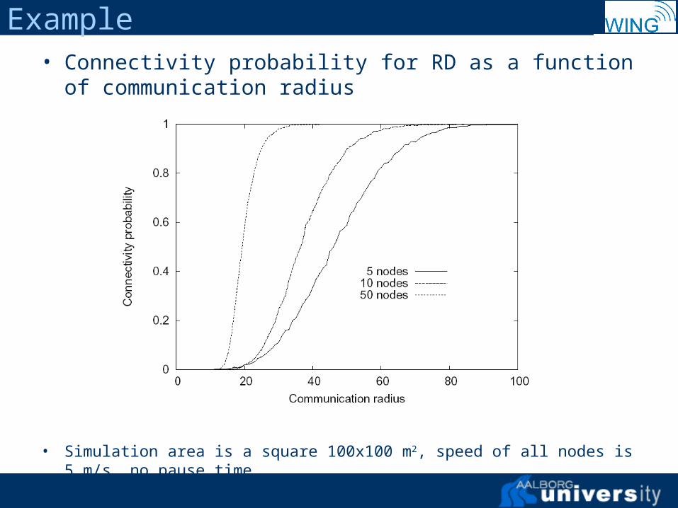
Example• Connectivity probability for RD as a function of

communication radius

• Simulation area is a square 100x100 m2, speed of all nodes is 5 m/s, no pause time

Computational Effort

• area 100x100 m• comm. radius 20m• 90 nodes• speed 5 m/s• Conn. probability = approx. 0.87• Using formula

– N=2000 cpu time=132 sec

– N=10.000 cpu time=666 sec

• Using definition – t=5.000 sec cpu time = 2431 sec

– t=10.000 sec cpu time = 5476 sec

Applicability of the method to other models• The same formula is applicable in the case of

– general RD model

– When rectangular-shaped obstacles are placed in the simulation area

• If a collection of nodes comprises a dynamical system with some particular properties, then for almost all initial conditions the limit exists. It can happen that for different initial positions and velocities, the limiting values will be different.

• Note that for RD model the limit does not depend on initial conditions, therefore it is defined correctly.

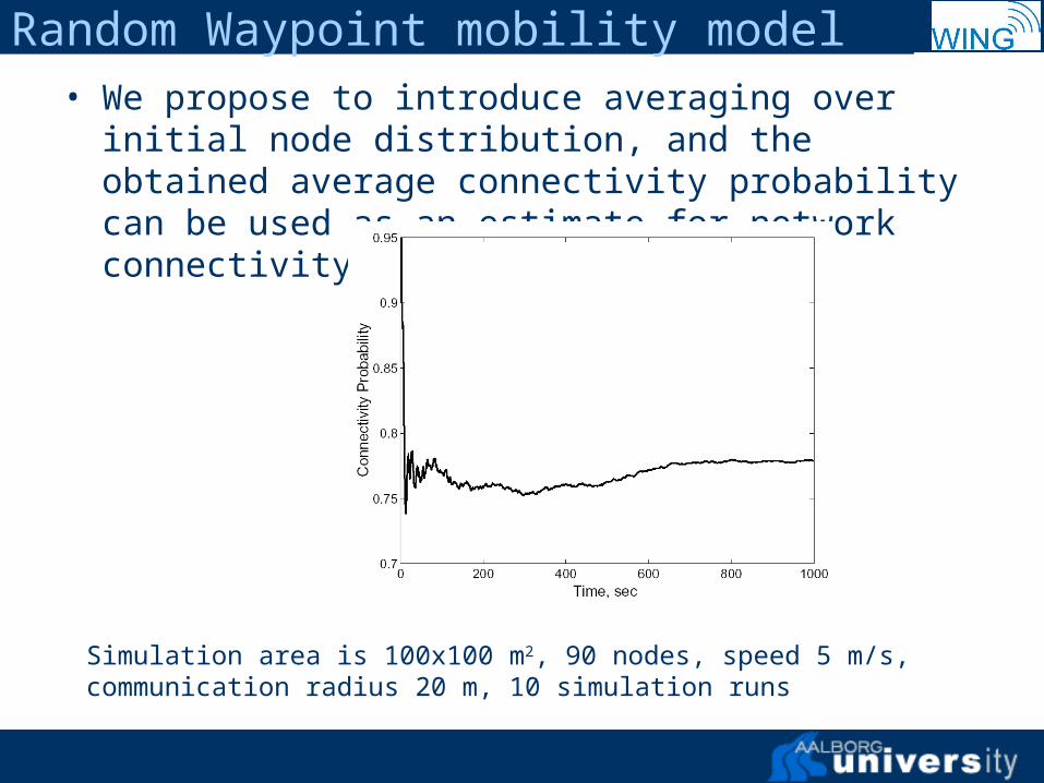
Random Waypoint mobility model• We propose to introduce averaging over initial node

distribution, and the obtained average connectivity probability can be used as an estimate for network connectivity.

Simulation area is 100x100 m2, 90 nodes, speed 5 m/s, communication radius 20 m, 10 simulation runs

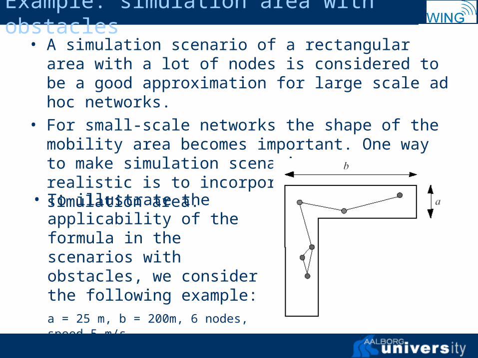
Example: simulation area with obstacles • A simulation scenario of a rectangular area with a lot of

nodes is considered to be a good approximation for large scale ad hoc networks.

• For small-scale networks the shape of the mobility area becomes important. One way to make simulation scenarios more realistic is to incorporate obstacles simulation area.

• To illustrate the applicability of the formula in the scenarios with obstacles, we consider the following example:a = 25 m, b = 200m, 6 nodes, speed 5 m/s

Example: simulation area with obstacles• Connectivity probability for RD as a function of communication

radius

• Line A: we propose use a simplified propagation model: a signal can reach the receiver via non LOS mechanism, but the receiving power is 20 dB smaller compared with the case when a LOS path exists.

• The number 20 dB seems to be realistic for indoor environment, but it can vary a lot depending on materials of walls and ceiling, size of the room etc

Conclusions and future work• We have presented a new method to describe

connectivity of a network in presence of mobility as a measure

• The developed framework was applied to Random Direction model; it’s applicability to other models was discussed

• In the future we plan to examine other mobility models, including the one, based on the use of mobility trajectories of the users in a virtual world using a multi-player game such as e.g. Quake II.