Full Terms & Conditions of access and use can be found athttp://www.tandfonline.com/action/journalInformation?journalCode=tprs20

Download by: [Tsinghua University] Date: 07 June 2016, At: 18:08

International Journal of Production Research

ISSN: 0020-7543 (Print) 1366-588X (Online) Journal homepage: http://www.tandfonline.com/loi/tprs20

Impact of demand price elasticity on advantagesof cooperative advertising in a two-tier supplychain

Lei Zhao, Jihua Zhang & Jinxing Xie

To cite this article: Lei Zhao, Jihua Zhang & Jinxing Xie (2016) Impact of demand price elasticityon advantages of cooperative advertising in a two-tier supply chain, International Journal ofProduction Research, 54:9, 2541-2551, DOI: 10.1080/00207543.2015.1096978

To link to this article: http://dx.doi.org/10.1080/00207543.2015.1096978

Published online: 15 Oct 2015.

Submit your article to this journal

Article views: 114

View related articles

View Crossmark data

Impact of demand price elasticity on advantages of cooperative advertising in a two-tiersupply chain

Lei Zhao, Jihua Zhang and Jinxing Xie*

Department of Mathematical Sciences, Tsinghua University, Beijing, China

(Received 21 January 2015; accepted 16 September 2015)

This paper focuses on pricing and vertical cooperative advertising decisions in a two-tier supply chain. Using aStackelberg game model where the manufacturer acts as the game leader and the retailer acts as the game follower, weobtain closed-form equilibrium solution and explicitly show how pricing and advertising decisions are made. Whenmarket demand decreases exponentially with respect to the retail price and increases with respect to national and localadvertising expenditures in an additive way, the manufacturer benefits from providing percentage reimbursement for theretailer’s local advertising expenditure when demand price elasticity is large enough. Whether the manufacturer benefitsfrom cooperative advertising is also closely related to supply chain member’s relative advertising efficiency. In thedecision for adopting coop advertising strategy, it is critical for the manufacturer to identify how market demand dependson national and local advertisements. The findings from this research can enhance our understanding of cooperativeadvertising decisions in a two-tier supply chain with price-dependent demand.

Keywords: cooperative advertising; pricing; game theory; supply chain management

1. Introduction

When market demand of a certain product is advertising dependent, both national advertising and local advertising playa role. National advertising is usually brand name oriented and aims at enlarging potential client base, whereas localadvertising is end customer oriented and is basically used to stimulate short-term sales. In a typical two-tier supplychain, national advertising is usually undertaken by the upstream member (the manufacturer) and local advertising isusually undertaken by the downstream member (the retailer). Vertical cooperative (coop) advertising is an arrangementin which the manufacturer shares a portion of the retailer’s local advertising cost. The fraction shared is referred to asthe (manufacturer’s) participation rate. In the absence of coop advertising, the retailer would typically advertise less thanthat desired by the manufacturer. Thus, participation rates, as well as supply chain members’ advertising expenditures,are fundamental decisions in a supply chain. Many studies about coop advertising and various extensions have been pre-sented in the literature (Berger 1972; Jørgensen and Zaccour 1999, 2003; Huang and Li 2001; Karray and Zaccour2007; Wang et al. 2011; He et al. 2011, 2012; Ahmadi-Javid and Hoseinpour 2012; Zhang et al. 2013; Aust andBuscher 2014a; Gou et al. 2014; Karray and Amin 2015). Recently, Jørgensen and Zaccour (2014) and Aust andBuscher (2014b) provide comprehensive reviews of researches on coop advertising.

Pricing is another fundamental decision in a supply chain. It typically includes decisions for the manufacturer’swholesale price and the retailer’s retail price. Both pricing and coop advertising are significant determinants of marketdemand and hence profits of both supply chain members. However, analytical models that simultaneously deal withcoop advertising and pricing decisions are relatively sparse. Karray and Zaccour (2006) allow price competition in theirmodel and address the coop advertising as an efficient counterstrategy for the manufacturer in the presence of the retai-ler’s private label. Yet, the manufacturer’s national advertising decision is not included in their model. Yue et al. (2006)incorporate demand price elasticity in the customer demand function, while the manufacturer, bypassing the retailer,directly gives the consumer a price deduction from the suggested retail price. However, their model takes neither whole-sale price nor retail price as supply chain member’s decision variables.

More recently, there is increasing research interest in analytical models that simultaneously deal with coop advertis-ing and pricing decisions. Assuming that market demand decreases exponentially with respect to the retail price andincreases with respect to national and local advertising expenditures in a multiplicative way, Szmerekovsky and Zhang

*Corresponding author. Email: jxie@math.tsinghua.edu.cn

© 2015 Informa UK Limited, trading as Taylor & Francis Group

International Journal of Production Research, 2016Vol. 54, No. 9, 2541–2551, http://dx.doi.org/10.1080/00207543.2015.1096978

Dow

nloa

ded

by [

Tsi

nghu

a U

nive

rsity

] at

18:

08 0

7 Ju

ne 2

016

(2009) show that it is optimal for the manufacturer not to provide reimbursement for the retailer’s local advertisingexpenditure. Xie and Neyret (2009), Xie and Wei (2009) and Yan (2010) assume that the demand decreases linearlywith respect to the retail price and find that the manufacturer usually benefits from providing percentage reimbursementfor the retailer’s local advertising expenditure. SeyedEsfahani, Biazaran, and Gharakhani (2011) introduce a demandfunction with a new parameter that can induce either a convex or a concave demand curve. Aust and Buscher (2012)extend the work by relaxing restrictions on the ratio between the manufacturer’s and the retailer’s profit margins. Acommon assumption made in these studies is that the demand function is multiplicatively separable in advertisementand price. Besides, all these studies adopt a deterministic and static game model, which implicitly assumes that players(firms) make decisions for a single-period problem. There are also stochastic and dynamic models that deal withthe advertising goodwill evolution. For example, He, Prasad, and Sethi (2009) propose a stochastic Stackelbergdifferential game and provide in the feedback form the optimal advertising and pricing policies for the manufacturerand the retailer.

This paper focuses on the deterministic and static game model only. Noticing that both the linear demand function(Xie and Neyret 2009; Xie and Wei 2009; Yan 2010) and the non-linear demand function (SeyedEsfahani, Biazaran,and Gharakhani 2011; Aust and Buscher 2012) in the abovementioned literature imply a non-constant price elasticity,while the exponential demand function (Szmerekovsky and Zhang 2009) reflects a constant price elasticity, we are inter-ested in the following question: What’s the impact of demand price elasticity on the manufacturer’s decision on coopera-tive advertising? Specifically, assuming market demand decreases exponentially with respect to the retail price andincreases with respect to national and local advertising expenditures in an additive way, we find that the manufacturerbenefits from providing percentage reimbursement for the retailer’s local advertising when demand price elasticity is lar-ger than a certain value. Whether the manufacturer benefits from cost sharing is also related to supply chain members’relative advertising efficiency. These results can enhance our understanding about the coop advertising and pricingdecisions in a two-tier supply chain.

The remainder of this paper is organised as follows: Section 2 presents the model and assumptions. Section 3 solvesthe unique equilibrium for the Stackelberg game. Section 4 does sensitive analysis regarding impacts of different param-eters on the equilibrium pricing and coop advertising decisions. Section 5 concludes the paper and proposes futureresearch directions.

2. Model and assumptions

Consider a two-tier supply chain consisting of a single manufacturer and a single retailer, in which they play a sequen-tial Stackelberg game. At the first stage of the game, the manufacturer acts as the game leader and decides the wholesaleprice w (w > 0), the national advertising expenditure A (A ≥ 0) and the participation rate t (0 ≤ t < 1) simultaneously. Atthe second stage of the game, the retailer acts as the game follower and decides the local advertising expenditure a(a ≥ 0) and meanwhile sets the retail price p (p ≥ w).

Assume market demand V depends jointly on a, A and p as follows:

V ðp; a;AÞ ¼ p�eðkrffiffiffia

p þ kmffiffiffiA

pÞ (1)

where e is the demand price elasticity and kr and km are positive parameters taking account of the different effectivenessof local and national advertising expenditures. Equation (1) implies that market demand depends on pricing effect (p−e)and advertising effect (kr

ffiffiffia

p þ kmffiffiffiA

p) in a multiplicative pattern, which is in accord with most of the existing studies

(e.g. Xie and Wei 2009; Aust and Buscher 2012). As in Szmerekovsky and Zhang (2009), we assume e > 1, so thedemand is exponentially decreasing with respect to p. In order to simplify expositions, we define the advertising ratio ask ¼ k2m=k

2r .

Let the manufacturer’s unit production cost be C (C > 0), then we can write the profit functions for the manufacturerand the retailer as follows:

Pm ¼ ðw� CÞp�eðkrffiffiffia

p þ kmffiffiffiA

pÞ � ta� A; (2)

Pr ¼ ðp� wÞp�eðkrffiffiffia

p þ kmffiffiffiA

pÞ � ð1� tÞa: (3)

2542 L. Zhao et al.

Dow

nloa

ded

by [

Tsi

nghu

a U

nive

rsity

] at

18:

08 0

7 Ju

ne 2

016

3. Stackelberg equilibrium

In this section, we solve the Stackelberg game and obtain the equilibrium solution by backward induction. At the secondstage of the game, with the variables A, w and t being given, the retailer faces the following decision problem:

Max Pr ¼ ðp� wÞp�eðkrffiffiffia

p þ kmffiffiffiA

p Þ � ð1� tÞas.t. p�w and a� 0:

(4)

Although the objective function Πr may not be jointly concave with respect to the decision variables a and p, the partic-ular function form allows to obtain a closed-form solution to the optimisation problem. Specifically, it is straightforwardto calculate

@Pr=@p ¼ p�e�1ðkrffiffiffia

p þ kmffiffiffiA

pÞ½ew� ðe� 1Þp�: (5)

with the assumption e > 1, the retailer’s profit Πr will increase in p when w ≤ p ≤ ew/(e − 1) and decrease in p whenp ≥ ew/(e − 1). This justifies that the optimal retail price for the retailer should be

p ¼ ew=ðe� 1Þ; (6)

for all a ≥ 0, A ≥ 0, w ≥ C and 0 ≤ t < 1.Equation (6) indicates that the retail price (p) should be set proportionally to the wholesale price (w), with the pro-

portional coefficient e/(e − 1) being a decreasing function of the demand price elasticity (e). But it does not explicitlydepend on the variables A, t and a and the parameters kr and km.

It is easy to check whether Πr is a concave function with respect to a. By setting ∂Πr/∂a = 0, we can obtain theretailer’s optimal local advertising expenditure as

a ¼ k2r p�2eðp� wÞ2=4ð1� tÞ2: (7)

Equation (7) holds for all p ≥ w. Substituting (6) into (7), we have

a ¼ k2r ½ew=ðe� 1Þ�2�2e=4e2ð1� tÞ2: (8)

Equation (8) indicates that the local advertising expenditure (a) should be set as a decreasing function of the wholesaleprice (w),and as an increasing function of the participation rate (t). But the national advertising expenditure (A) does notexplicitly impact the decision for the local advertising expenditure (a).

Therefore, at the first stage of the game, the manufacturer faces the following decision problem:

Max Pm ¼ ðw� CÞp�eðkrffiffiffia

p þ kmffiffiffiA

p Þ � ta� As.t. 0� t\1;w�C; and A� 0;

(9)

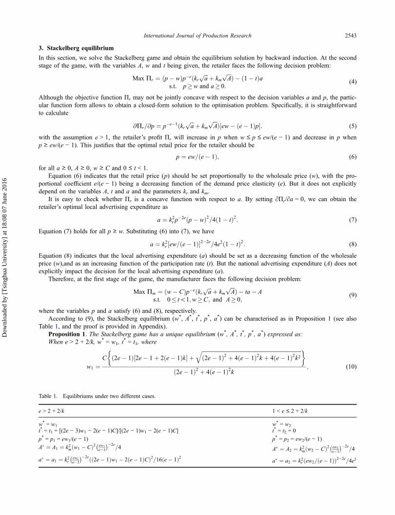
where the variables p and a satisfy (6) and (8), respectively.According to (9), the Stackelberg equilibrium (w*, A*, t*, p*, a*) can be characterised as in Proposition 1 (see also

Table 1, and the proof is provided in Appendix).Proposition 1. The Stackelberg game has a unique equilibrium (w*, A*, t*, p*, a*) expressed as:When e > 2 + 2/k, w* = w1, t

* = t1, where

w1 ¼C ð2e� 1Þ½2e� 1þ 2ðe� 1Þk� þ

ffiffiffiffiffiffiffiffiffiffiffiffiffiffiffiffiffiffiffiffiffiffiffiffiffiffiffiffiffiffiffiffiffiffiffiffiffiffiffiffiffiffiffiffiffiffiffiffiffiffiffiffiffiffiffiffiffiffiffiffiffiffiffiffiffiffiffiffiffiffiffiffiffiffið2e� 1Þ2 þ 4ðe� 1Þ2k þ 4ðe� 1Þ2k2

q� �

ð2e� 1Þ2 þ 4ðe� 1Þ2k ; (10)

Table 1. Equilibriums under two different cases.

e > 2 + 2/k 1 < e ≤ 2 + 2/k

w* = w1 w* = w2

t* = t1 = [(2e − 3)w1 − 2(e − 1)C]/[(2e − 1)w1 − 2(e − 1)C] t* = t2 = 0

p* = p1 = ew1/(e − 1) p* = p2 = ew2/(e − 1)

A� ¼ A1 ¼ k2mðw1 � CÞ2 ew1e�1

� ��2e=4 A� ¼ A2 ¼ k2mðw2 � CÞ2 ew2

e�1

� ��2e=4

a� ¼ a1 ¼ k2rew1e�1

� ��2eðð2e� 1Þw1 � 2ðe� 1ÞCÞ2=16ðe� 1Þ2 a� ¼ a2 ¼ k2r ðew2=ðe� 1ÞÞ2�2e=4e2

International Journal of Production Research 2543

Dow

nloa

ded

by [

Tsi

nghu

a U

nive

rsity

] at

18:

08 0

7 Ju

ne 2

016

t1 ¼ ð2e� 3Þw� � 2ðe� 1ÞCð2e� 1Þw� � 2ðe� 1ÞC : (11)

When e ≤ 2 + 2/k, w* = w2, t* = t2, where

w2 ¼C ð2e� 1Þ½1þ ðe� 1Þk� þ

ffiffiffiffiffiffiffiffiffiffiffiffiffiffiffiffiffiffiffiffiffiffiffiffiffiffiffiffiffiffiffiffiffiffiffiffiffiffiffiffiffiffiffiffiffiffiffiffiffiffiffiffiffiffiffiffiffiffiffiffiffiffiffiffiffiffiffiffiffið2e� 1Þ2 þ 2ðe� 1Þk þ ðe� 1Þ2k2

q� �

2ðe� 1Þ½2þ ðe� 1Þk� ; (12)

t2 ¼ 0: (13)

Under both cases, after the values for (w*, t*) are determined, the values for (A*, p*, a*) can be calculated as:

A� ¼ k2mðw� � CÞ2 ew�

e� 1

� ��2e

=4; (14)

p� ¼ ew�=ðe� 1Þ; (15)

a� ¼ k2r ½ew�=ðe� 1Þ�2�2e=4e2ð1� t�Þ2: (16)

Proposition 1 reveals that under our assumptions for the demand function, the manufacturer has no incentive to sharethe retailer’s local advertising expenditure when the price elasticity is smaller than a certain value. However, when theprice elasticity is larger than a certain value, the manufacturer benefits from providing percentage reimbursement for theretailer’s local advertising expenditure. This result is different from that in Szmerekovsky and Zhang (2009). Assumingthe demand function takes the form of V(p, a, A) = p−e(α − βa−γA−δ) (e > 1 and α, β, γ, δ are positive constants), theyfind that for all values of price elasticity greater than 1, the optimal strategy for the manufacturer is not to provide anysubsidy to the retailer’s local advertisement. This difference is due to the different assumptions about the effect of adver-tisements on the demand. National and local advertisements are assumed to increase market demand in a multiplicativeway in their model, while they are assumed to work in an additive way in our model. These two different findings com-plement each other and suggest that when the manufacturer considers whether coop advertising strategy should beadopted, it is critical to identify how the demand depends on national and local advertisements.

Usually, products with many substitutes or whose purchase can be easily postponed, or that are considered luxuriesother than essential to everyday living, have higher price elasticities. For example, the demand for a specific brand softdrink would likely be highly elastic, and its price elasticity can be more than 4 (Ayers and Collinge 2005). Similarly,goods and services include specific-model automobiles, fresh tomatoes and long-run foreign travels. (Gwartney et al.2014). For these industries, if national advertising and local advertising increase market demand in an additive way asin our model, our result suggests that coop advertising strategy will be very attractive to the goods manufacturers (orservice providers).

Now we focus on the case where the price elasticity is large enough (i.e. e > 2 + 2/k), so that the manufacturer’soptimal strategy is to provide a positive reimbursement to the retailer’s local advertising expenditure. If the manufacturermakes a wrong decision and provides no reimbursement for the retailer’s local advertising expenditure, his optimal strat-egy is to use t* = t2 = 0, and the associated optimal wholesale price is obtained by w* = w2, as expressed in (12). How-ever, when he provides a positive reimbursement to the retailer’s local advertising expenditure, his optimal strategy is touse t* = t1 and w* = w1, as expressed in (10) and (11). Obviously, the reimbursement from the manufacturer will inducethe retailer to invest more on local advertising, i.e. a1 > a2. The following proposition reveals the impact of the decisionmistake on other decision variables (the wholesale price, the retail price and the manufacturer’s national advertisingexpenditure).

Proposition 2. Suppose e > 2 + 2/k, then w1 > w2, A1 > A2, p1 > p2, a1 > a2.Proposition 2 concludes that when e > 2 + 2/k, if the manufacturer provides no reimbursement for the retailer’s local

advertising expenditure, the retailer will invest less on national advertising and the manufacturer will also invest less onnational advertising. Thus, the demand generated from both advertising will be lower. In order to maximise his profit,the retailer has to announce a lower retail price to induce more sales. Similarly, the manufacturer should also charge alower wholesale price. This leads to low profit margins for both the manufacturer and the retailer, resulting in a lose-lose situation for both supply chain members. On the contrary, by adopting coop advertising, the demand generatedfrom advertising will be higher and both the supply chain members can increase their profit margins and improve theperformance of the supply chain.

2544 L. Zhao et al.

Dow

nloa

ded

by [

Tsi

nghu

a U

nive

rsity

] at

18:

08 0

7 Ju

ne 2

016

4. Effects of demand parameters on the pricing and coop advertising decisions

In this section, we concentrate our discussions on the case where the price elasticity is large enough (i.e. e > 2 + 2/k),so that the manufacturer’s optimal strategy is to provide a positive reimbursement to the retailer’s local advertising cost.Proposition 3 summaries how the manufacturer’s and retailer’s decision variables will be influenced by the parametersof the model.

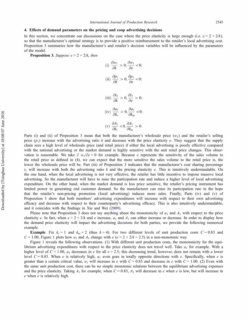
Proposition 3. Suppose e > 2 + 2/k, then

ðiÞ @w1

@k[ 0;

@w1

@e\0;

ðiiÞ @p1@k

[ 0;@p1@e

\0;

ðiiiÞ @t1@k

[ 0;@t1@e

[ 0;

ðivÞ @a1@kr

[ 0;@a1@km

\0;

ðvÞ @A1

@kr\0;

@A1

@km[ 0:

Parts (i) and (ii) of Proposition 3 mean that both the manufacturer’s wholesale price (w1) and the retailer’s sellingprice (p1) increase with the advertising ratio k and decrease with the price elasticity e. They suggest that the supplychain sees a high level of wholesale price (and retail price) if either the local advertising is poorly effective comparedwith the national advertising or the market demand is highly sensitive with the unit retail price changes. This obser-vation is reasonable. We take ∂ w1/∂e < 0 for example. Because e represents the sensitivity of the sales volume tothe retail price as defined in (4), we can expect that the more sensitive the sales volume to the retail price is, thelower the wholesale price will be. Part (iii) of Proposition 3 indicates that the manufacturer’s cost sharing percentaget1 will increase with both the advertising ratio k and the pricing elasticity e. This is intuitively understandable. Onthe one hand, when the local advertising is not very effective, the retailer has little incentive to impose massive localadvertising. So the manufacturer will have to raise the participation rate and induce a higher level of local advertisingexpenditure. On the other hand, when the market demand is less price sensitive, the retailer’s pricing instrument haslimited power in generating end customer demand. So the manufacturer can raise its participation rate in the hopethat the retailer’s non-pricing promotion (local advertising) induces more sales. Finally, Parts (iv) and (v) ofProposition 3 show that both members’ advertising expenditures will increase with respect to their own advertisingefficacy and decrease with respect to their counterparty’s advertising efficacy. This is also intuitively understandable,and it coincides with the findings in Xie and Wei (2009).

Please note that Proposition 3 does not say anything about the monotonicity of a1 and A1 with respect to the priceelasticity e. In fact, when e > 2 + 2/k and e increase, a1 and A1 can either increase or decrease. In order to display howthe demand price elasticity will impact the advertising decisions for both parties, we provide the following numericalexample.

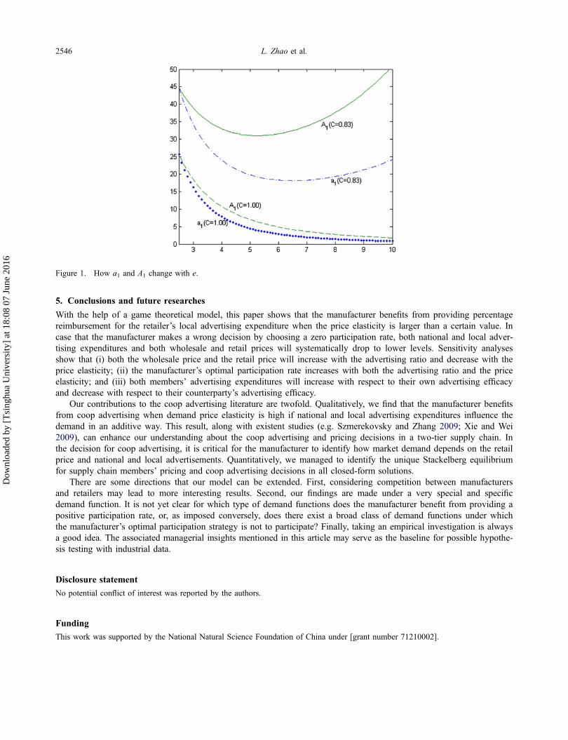
Example. Fix kr = 1 and km = 2 (thus k = 4). For two different levels of unit production costs C = 0.83 andC = 1.00, Figure 1 plots how a1 and A1 change with e (e > 2 + 2/k = 2.5) in a non-monotonic way.

Figure 1 reveals the following observations. (1) With different unit production costs, the monotonicity for the equi-librium advertising expenditures with respect to the price elasticity does not travel well. Take a1 for example. With ahigher level of C = 1.00, a1 decreases in e for all e > 2.5; this decreasing trend, however, does not remain with a lowerlevel C = 0.83. When e is relatively high, a1 even goes in totally opposite directions with e. Specifically, when e isgreater than a certain critical value, a1 will increase in e with C = 0.83 and decrease in e with C = 1.00. (2) Even withthe same unit production cost, there can be no simple monotonic relations between the equilibrium advertising expensesand the price elasticity. Taking A1 for example, when C = 0.83, A1 will decrease in e when e is low, but will increase ine when e is relatively high.

International Journal of Production Research 2545

Dow

nloa

ded

by [

Tsi

nghu

a U

nive

rsity

] at

18:

08 0

7 Ju

ne 2

016

5. Conclusions and future researches

With the help of a game theoretical model, this paper shows that the manufacturer benefits from providing percentagereimbursement for the retailer’s local advertising expenditure when the price elasticity is larger than a certain value. Incase that the manufacturer makes a wrong decision by choosing a zero participation rate, both national and local adver-tising expenditures and both wholesale and retail prices will systematically drop to lower levels. Sensitivity analysesshow that (i) both the wholesale price and the retail price will increase with the advertising ratio and decrease with theprice elasticity; (ii) the manufacturer’s optimal participation rate increases with both the advertising ratio and the priceelasticity; and (iii) both members’ advertising expenditures will increase with respect to their own advertising efficacyand decrease with respect to their counterparty’s advertising efficacy.

Our contributions to the coop advertising literature are twofold. Qualitatively, we find that the manufacturer benefitsfrom coop advertising when demand price elasticity is high if national and local advertising expenditures influence thedemand in an additive way. This result, along with existent studies (e.g. Szmerekovsky and Zhang 2009; Xie and Wei2009), can enhance our understanding about the coop advertising and pricing decisions in a two-tier supply chain. Inthe decision for coop advertising, it is critical for the manufacturer to identify how market demand depends on the retailprice and national and local advertisements. Quantitatively, we managed to identify the unique Stackelberg equilibriumfor supply chain members’ pricing and coop advertising decisions in all closed-form solutions.

There are some directions that our model can be extended. First, considering competition between manufacturersand retailers may lead to more interesting results. Second, our findings are made under a very special and specificdemand function. It is not yet clear for which type of demand functions does the manufacturer benefit from providing apositive participation rate, or, as imposed conversely, does there exist a broad class of demand functions under whichthe manufacturer’s optimal participation strategy is not to participate? Finally, taking an empirical investigation is alwaysa good idea. The associated managerial insights mentioned in this article may serve as the baseline for possible hypothe-sis testing with industrial data.

Disclosure statement

No potential conflict of interest was reported by the authors.

Funding

This work was supported by the National Natural Science Foundation of China under [grant number 71210002].

Figure 1. How a1 and A1 change with e.

2546 L. Zhao et al.

Dow

nloa

ded

by [

Tsi

nghu

a U

nive

rsity

] at

18:

08 0

7 Ju

ne 2

016

References

Ahmadi-Javid, A., and P. Hoseinpour. 2012. “On a Cooperative Advertising Model for a Supply Chain with One Manufacturer andOne Retailer.” European Journal of Operational Research 219: 458–466.

Aust, G., and U. Buscher. 2012. “Vertical Cooperative Advertising and Pricing Decisions in a Manufacturer–Retailer Supply Chain:A Game-theoretical Approach.” European Journal of Operational Research 223: 473–482.

Aust, G., and U. Buscher. 2014a. “Vertical Cooperative Advertising in a Retailer Duopoly.” Computers & Industrial Engineering 72:247–254.

Aust, G., and U. Buscher. 2014b. “Cooperative Advertising Models in Supply Chain Management: A Review.” European Journal ofOperational Research 234: 1–14.

Ayers, R., and R. Collinge. 2005. Microeconomics: Explore and Apply. Upper Saddle River, NJ: Pearson Prentice Hall.Berger, P. D. 1972. “Vertical Cooperative Advertising Ventures.” Journal of Marketing Research 9: 309–312.Gou, Q., J. Zhang, L. Liang, Z. Huang, and A. Ashley. 2014. “Horizontal Cooperative Programmes and Cooperative Advertising.”

International Journal of Production Research 52 (3): 691–712.Gwartney, J., R. Stroup, R. Sobel, and D. Macpherson. 2014. Economics: Private and Public Choice. Mason, OH: Cengage Learning.He, X., A. Prasad, and S. P. Sethi. 2009. “Co-op Advertising and Pricing in a Stochastic Supply Chain: Feedback Stackelberg Strate-

gies.” Production and Operations Management 18 (1): 78–94.He, X., A. Krishnamoorthy, A. Prasad, and S. P. Sethi. 2011. “Retail Competition and Cooperative Advertising.” Operations Research

Letters 39 (1): 11–16.He, X., A. Krishnamoorthy, A. Prasad, and S. P. Sethi. 2012. “Co-op Advertising in Dynamic Retail Oligopolies.” Decision Sciences

43 (1): 73–106.Huang, Z., and S. X. Li. 2001. “Coop Advertising Models in a Manufacturer–Retailer Supply Chain: A Game Theory Approach.”

European Journal of Operational Research 135 (3): 527–544.Jorgensen, S., and G. Zaccour. 1999. “Equilibrium Pricing and Advertising Strategies in a Marketing Channel.” Journal of Optimiza-

tion Theory and Applications 102: 111–125.Jorgensen, S., and G. Zaccour. 2003. “Channel Coordination Over Time: Incentive Equilibria and Credibility.” Journal of Economic

Dynamics and Control 27: 801–822.Jorgensen, S., and G. Zaccour. 2014. “A Survey of Game-theoretical Models of Cooperative Advertising.” European Journal of

Operational Research 237: 1–14.Karray, S., and S. H. Amin. 2015. “Cooperative Advertising in a Supply Chain with Retail Competition.” International Journal of

Production Research 53 (1): 88–105.Karray, S., and G. Zaccour. 2006. “Could Co-op Advertising be a Manufacturer’s Counterstrategy to Store Brands?” Journal of

Business Research 59 (9): 1008–1015.Karray, S., and G. Zaccour. 2007. “Effectiveness of Coop Advertising Programs in Competitive Distribution Channels.” International

Game Theory Review 9 (2): 151–167.SeyedEsfahani, M. M., M. Biazaran, and M. Gharakhani. 2011. “A game Theoretic Approach to Coordinate Pricing and Vertical

Co-op Advertising in Manufacturer–Retailer Supply Chains.” European Journal of Operational Research 211 (2): 263–273.Szmerekovsky, J. G., and J. Zhang. 2009. “Pricing and Two-tier Advertising with One Manufacturer and One Retailer.” European

Journal of Operational Research 192 (3): 904–917.Wang, S., Y. Zhou, J. Min, and Y. Zhong. 2011. “Coordination of Cooperative Advertising Models in a One-manufacturer Two-

retailer Supply Chain System.” Computers & Industrial Engineering 61 (4): 1053–1071.Xie, J., and A. Neyret. 2009. “Co-op Advertising and Pricing Models in Manufacturer–Retailer Supply Chains Co-op Advertising and

Pricing Models in Manufacturer–Retailer Supply Chains.” Computers & Industrial Engineering 56 (4): 1375–1385.Xie, J., and J. C. Wei. 2009. “Coordinating Advertising and Pricing in a Manufacturer–Retailer Channel.” European Journal of

Operational Research 197 (2): 785–791.Yan, R. 2010. “Cooperative Advertising, Pricing Strategy and Firm Performance in the E-Marketing Age.” Journal of the Academy of

Marketing Science 38 (4): 510–519.Yue, J., J. Austin, M. Wang, and Z. Huang. 2006. “Coordination of Cooperative Advertising in a Two-level Supply Chain When

Manufacturer Offers Discount.” European Journal of Operational Research 168 (1): 65–85.Zhang, J., Q. Gou, L. Liang, and X. He. 2013. “Ingredient Branding Strategies in an Assembly Supply Chain: Models and Analysis.”

International Journal of Production Research 51 (23–24): 6923–6949.

International Journal of Production Research 2547

Dow

nloa

ded

by [

Tsi

nghu

a U

nive

rsity

] at

18:

08 0

7 Ju

ne 2

016

Appendix 1

A.1 Proof of Proposition 1Substituting Equations (6) and (8) into the expression of Πm, the manufacturer’s decision problem (9) becomes

Max Pm ¼ ðw� CÞ ew

e� 1

�e k2rew

e� 1

1�e

2e 1� tð Þ þ kmffiffiffiA

p0B@

1CA�

tk2rew

e� 1

2�2e

4e2 1� tð Þ2 � A

s.t. 0� t\1;w�C and A� 0:

(A.1)

In order to determine the unique optimal solution (w*, t*, A*), we first examine the manufacturer’s optimal decision on the nationaladvertising expenditure. Noticing @2Pm=@A2 ¼ � 1

4 kmðw� CÞ ew=ðe�1Þ� ��e

A�3=2 � 0 and w ≥ C, we know Πm is a concave functionwith respect to A for all A ≥ 0. Thus, we can solve the first-order condition ∂Πm/ ∂A = 0 and uniquely obtain the optimal nationaladvertising expenditure by

A ¼ k2mðw� CÞ2 ew

e� 1

�2e=4: (A.2)

Substituting (A.2) into (A.1), we reduce the manufacturer’s maximisation problem to

fMax Pmðw; tÞ; s.t. 0� t\1;w�Cg;where Pmðw; tÞ ¼

ðw� CÞ ew

e� 1

�e k2rew

e� 1

1�e

2e 1� tð Þ þ k2mðw� CÞ ewe�1

� ��e

2

264

375�

tk2rew

e� 1

2�2e

4e2 1� tð Þ2 �k2mðw� CÞ2 ew

e� 1

�2e

4(A.3)

Next we consider the manufacturer’s optimal decisions on t and w.(i) Consider the case with e > 2 + 2/k.The first-order derivative of Pmðw; tÞ with respect to t is given by

@Pmðw; tÞ@t

¼ k2r½ð1� 2eÞwþ 2Cðe� 1Þ�t þ ð2e� 3Þw� 2Cðe� 1Þ

4ð1� tÞ3e2ew2e�1ðe� 1Þ2�2e : (A.4)

With the constraints 0 ≤ t < 1 and w ≥ C, the sign of the derivative (A.4) is determined by the formula f(t) = [(1 − 2e)w + 2(e − 1)C]t + (2e − 3)w − 2(e − 1)C, which is a decreasing function in t since the slope (1 − 2e)w + 2(e − 1)C ≤ [(1 − 2e) + 2(e − 1)]C = −C < 0. We define t0 = [(2e − 3)w − 2(e − 1)C]/[(2e − 1)w − 2(e − 1)C] such that f(t0) = 0, then f(t) will be positive for t < t0and negative for t > t0. Taking the constraint 0 ≤ t < 1 into consideration, two subcases will follow as below.

Subcase [I]. If f(0) > 0, or equivalently w > C(2e − 2)/(2e − 3), then f(t) will be positive for 0 ≤ t < t0 and negative for t0 < t < 1,which suggests that Pmðw; tÞ will first increase in t for 0 ≤ t < t0 and then decrease in t for t0 < t < 1. Thus, the manufacturer’soptimal choice of t should be given by

t½I�ðwÞ ¼ t0 ¼ ð2e� 3Þw� 2ðe� 1ÞCð2e� 1Þw� 2ðe� 1ÞC : (A.5)

Substituting (A.5) into (A.3), the manufacturer’s optimisation problem is now further reduced tofMax P½I�

m ðwÞ; s.t. w[Cð2e� 2Þ=ð2e� 3Þg,where

P½I�m ðwÞ ¼

ðe� 1Þ2e�2

16ðewÞ2e k2r ½2ðw� CÞðe� 1Þ þ w�2 þ 4k2mðw� CÞ2ðe� 1Þ2n o

(A.6)

is a function of the decision variable w only.Taking @P½I�

m ðwÞ=@w ¼ 0, and making use of k ¼ k2m=k2r , after some algebraic simplifications, we have

�½ð2e� 1Þ2 þ 4ðe� 1Þ2k�w2 þ 2ð2e� 1Þ½ð2e� 1Þ þ 2ðe� 1Þk�Cw� 4eðe� 1Þðk þ 1ÞC2 ¼ 0: (A.7)

The left-hand side of (A.7) is a quadratic and concave function that has two real roots given as follows:

w½I� ¼ C ð2e� 1Þ½ð2e� 1Þ þ 2ðe� 1Þk� þ ffiffiffiffiffiffiD1

p� �ð2e� 1Þ2 þ 4ðe� 1Þ2k ; (A.8)

�w½I� ¼C ð2e� 1Þ½ð2e� 1Þ þ 2ðe� 1Þk� � ffiffiffiffi

Dp

1

n oð2e� 1Þ2 þ 4ðe� 1Þ2k ; (A.9)

where

D1 ¼ ð2e� 1Þ2 þ 4ðe� 1Þ2k þ 4ðe� 1Þ2k2: (A.10)

2548 L. Zhao et al.

Dow

nloa

ded

by [

Tsi

nghu

a U

nive

rsity

] at

18:

08 0

7 Ju

ne 2

016

It is easy to verify that �w½I�\C\Cð2e� 2Þ=ð2e� 3Þ. Furthermore, we have

w½I� � 2Cðe� 1Þ=ð2e� 3Þ ¼4Cðe� 1Þ½ð2e� 1Þ2 þ 4ðe� 1Þ2k�½ke� 2ðk þ 1Þ�

ð2e� 3Þ½ð2e� 1Þ2 þ 4ðe� 1Þ2k�½2kðe� 1Þ þ ð2e� 1Þ2 þ ð2e� 3Þ ffiffiffiffiffiffiD1

p �; (A.11)

which is greater than zero given our assumption e > 2 + 2/k. So, �w½I� < C < C(2e − 2)/(2e − 3) < w[I]. It follows that @P½I�m ðwÞ=@w

takes positive values when w 2 ðCð2e� 2Þ=ð2e� 3Þ;w½I�Þ and takes negative values when w 2 ðw½I�;þ1Þ, indicating that P½I�m ðwÞ

increases in w when C(2e − 2)/(2e − 3)<w < w[I] and decreases in w when w > w[I]. This argument concludes that the optimal whole-sale price under Subcase [I] should be w�½I� ¼ w½I� and the associated optimal participation rate should be t½I�ðw�½I�Þ.

Subcase [II]. If f(0) ≤ 0, or equivalently (C≤)w ≤ C(2e − 2)/(2e − 3), then f(t) ≤ 0 for all t (0 ≤ t < 1), i.e. Pmðt;wÞ is decreasingin t for all t. So, the optimal choice of t should be t[II] = 0. With t = t[II] = 0, the manufacturer’s optimisation problem is then reducedto:

Max P½II�m ðwÞ; s.t. ðC�Þw�Cð2e� 2Þ=ð2e� 3Þ,

where

P½II�m ðwÞ ¼ ðw� CÞ ew

e�1

� ��2e

4ðe� 1Þ 2k2r wþ k2mðe� 1Þðw� CÞ �: (A.12)

Taking @P½II�m ðwÞ=@w ¼ 0, and making use of k ¼ k2m=k

2r , after some algebraic simplifications, we have

� ðe� 1Þ½kðe� 1Þ þ 2�w2 � ð2e� 1Þ½kðe� 1Þ þ 1�wC þ eðe� 1ÞkC2� � ¼ 0: (A.13)

The left-hand side of (A.13) is again a quadratic and concave function of w with two real roots as follows:

w½II� ¼ C ð2e� 1Þ½1þ ðe� 1Þk� þ ffiffiffiffiffiffiD2

p� �2ðe� 1Þ½2þ ðe� 1Þk� ; (A.14)

�w½II� ¼ C ð2e� 1Þ½1þ ðe� 1Þk� � ffiffiffiffiffiffiD2

p� �2ðe� 1Þ½2þ ðe� 1Þk� ; (A.15)

where D2 ¼ ð2e� 1Þ2 þ 2ðe� 1Þk þ ðe� 1Þ2k2: (A.16)

It is easy to check that �w½II� < C < C(2e − 2)/(2e − 3) < w[II]. Then @P½II�m ðwÞ=@w takes positive values for all w in [C, C(2e − 2)/

(2e − 3)], which indicates that P½II�m ðwÞ is increasing in w for all C ≤ w ≤ C(2e − 2)/(2e − 3). This argument concludes that the opti-

mal wholesale price under Subcase [II] should be w�½II� ¼ Cð2e� 2Þ=ð2e� 3Þ, with the associated optimal participation rate t[II] = 0.In order to find the global optimal solution (w*, t*) for Pmðw; tÞ with the condition e > 2 + 2/k, we should compare the

manufacturer’s optimal profits

P½I�m ðw�½I�Þ ¼ Pmðw�½I�; t½I�ðw�½I�ÞÞ under Subcase [I] and

P½II�m ðw�½II�Þ ¼ Pmðw�½II�; t½II�Þ ¼ Pmðw�½II�; 0Þ under Subcase [II].

By definition, we have P½I�m ðw�½I�Þ ¼ Pmðw�½I�; t½I�ðw�½I�ÞÞ �Pmðw; t½I�ðwÞÞ for all w > 2C(e − 1)/(2e − 3). Since Πm(w, t) is a contin-

uous function in w, when w goes down to the lower bound 2C(e − 1)/(2e − 3), we have

Pmðw�½I�; t½I�ðw�½I�ÞÞ� limw!þ2Cðe�1Þ=ð2e�3Þ

Pmðw; t½I�ðwÞÞ¼ Pmðw�½II�; t½I�ðw�½II�ÞÞ ¼ Pmðw�½II�; 0Þ ¼ Pmðw�½II�; t½II�Þ;

(A.17)

which concludes that P½I�m ðw�½I�Þ �P½II�

m ðw�½II�Þ.Therefore, when e > 2 + 2/k, the optimal decision for the manufacturer should be w* = w[I] = w1 and t* = t[I] = t1, which justifies

Equations (10) and (11).(ii) Now we consider the case with e ≤ 2 + 2/k.By (A.4), the sign of the first-order derivative @Pmðw; tÞ=@t is determined by the formula f(t) = [(1 − 2e)w + 2(e − 1)C]

t + (2e − 3)w − 2(e − 1)C, which is decreasing in t for all w ≥ C. Recalling that t0 is defined such that f(t0) = 0, we have t0 > 0 if andonly if f(0) = (2e − 3)w − 2(e − 1)C > 0. Taking the constraint 0 ≤ t < 1 into consideration, we have three independent subcases asfollows.

Subcase [III]. If e ≤ 3/2, then f(0) = (2e − 3)w − 2(e − 1)C ≤ 0. Consequently, f(t) ≤ 0 for all t (0 ≤ t < 1), i.e. Pmðw; tÞ isdecreasing in t for all given values of w ≥ C. So the optimal choice of t in Subcase [III] should be t[III] = 0.

Subcase [IV]. If 3/2 < e(≤2 + 2/k) and f(0) = (2e − 3)w − 2(e − 1)C ≤ 0, or equivalently, w ≤ C(2e − 2)/(2e − 3), then we stillhave f(t) ≤ 0 for 0 ≤ t < 1, i.e. Pmðw; tÞ is decreasing in t for all given values of w such that C ≤ w ≤ C(2e − 2)/(2e − 3). For thissituation, the optimal choice of t is t[IV] = 0.

Subcase [V]. If 3/2 < e(≤2 + 2/k) and f(0) = (2e − 3)w − 2(e − 1)C > 0, or equivalently, w > C(2e − 2)/(2e − 3), then f(t) takespositive values for 0 ≤ t < t0 and negative values for t0 < t < 1. Therefore, Pmðw; tÞ will increase in t for 0 ≤ t < t0 and decrease in tfor t0 < t < 1. So the manufacturer’s optimal choice of t should be t½V� ¼ t0.

International Journal of Production Research 2549

Dow

nloa

ded

by [

Tsi

nghu

a U

nive

rsity

] at

18:

08 0

7 Ju

ne 2

016

Using similar arguments as in Part (i), by comparing all the three subcases listed above, we can show that when e ≤ 2 + 2/k, themanufacturer’s (globally) optimal participation rate should be zero, i.e. t* = 0 = t2. The optimal wholesale price should be

w� ¼C ð2e� 1Þ½1þ ðe� 1Þk� þ

ffiffiffiffiffiffiffiffiffiffiffiffiffiffiffiffiffiffiffiffiffiffiffiffiffiffiffiffiffiffiffiffiffiffiffiffiffiffiffiffiffiffiffiffiffiffiffiffiffiffiffiffiffiffiffiffiffiffiffiffiffiffiffiffiffiffiffiffiffiffið2e� 1Þ2 þ 2ðe� 1Þk þ ðe� 1Þ2k2

q� �

2ðe� 1Þ½2þ ðe� 1Þk� ¼ w2; (A.18)

which justifies Equations (12) and (13).This completes the proof.

A.2 Proof of Proposition 2By Equations (14)–(16), A1 > A2, p1 > p2, a1 > a2 can be easily verified if w1 > w2. Thus, it suffices to prove w1 > w2. Using expres-sions of w1 and w2 in (10) and (12), we have

C

w1¼

½ð2e� 1Þ2 þ 2kðe� 1Þð2e� 1Þ� �ffiffiffiffiffiffiffiffiffiffiffiffiffiffiffiffiffiffiffiffiffiffiffiffiffiffiffiffiffiffiffiffiffiffiffiffiffiffiffiffiffiffiffiffiffiffiffiffiffiffiffiffiffiffiffiffiffiffiffiffiffiffiffiffiffiffiffiffiffiffiffiffiffiffið2e� 1Þ2 þ 4kðe� 1Þ2 þ 4k2ðe� 1Þ2

q4eðe� 1Þð1þ kÞ ; (A.19)

C

w2¼

ð2e� 1Þ½1þ kðe� 1Þ� �ffiffiffiffiffiffiffiffiffiffiffiffiffiffiffiffiffiffiffiffiffiffiffiffiffiffiffiffiffiffiffiffiffiffiffiffiffiffiffiffiffiffiffiffiffiffiffiffiffiffiffiffiffiffiffiffiffiffiffiffiffiffiffiffiffiffiffiffiffiffið2e� 1Þ2 þ 2kðe� 1Þ þ k2ðe� 1Þ2

q2keðe� 1Þ : (A.20)

In order to show w1 > w2, we only need to prove Cw2

[ Cw1, which, after some algebraic simplifications, is equivalent to

(2e� 1)ð2þ kÞ þ kffiffiffiffiffiffiffiffiffiffiffiffiffiffiffiffiffiffiffiffiffiffiffiffiffiffiffiffiffiffiffiffiffiffiffiffiffiffiffiffiffiffiffiffiffiffiffiffiffiffiffiffiffiffiffiffiffiffiffiffiffiffiffiffiffiffiffiffiffiffiffiffiffiffið2e� 1Þ2 þ 4ðe� 1Þ2k þ 4ðe� 1Þ2k2

q

[ 2ð1þ kÞffiffiffiffiffiffiffiffiffiffiffiffiffiffiffiffiffiffiffiffiffiffiffiffiffiffiffiffiffiffiffiffiffiffiffiffiffiffiffiffiffiffiffiffiffiffiffiffiffiffiffiffiffiffiffiffiffiffiffiffiffiffiffiffiffiffiffiffiffiffið2e� 1Þ2 þ 2ðe� 1Þk þ ðe� 1Þ2k2

q : (A.21)

Squaring both sides, this inequality is equivalent to

(2e� 1)ð2þ kÞkffiffiffiffiffiffiffiffiffiffiffiffiffiffiffiffiffiffiffiffiffiffiffiffiffiffiffiffiffiffiffiffiffiffiffiffiffiffiffiffiffiffiffiffiffiffiffiffiffiffiffiffiffiffiffiffiffiffiffiffiffiffiffiffiffiffiffiffiffiffiffiffiffiffið2e� 1Þ2 þ 4ðe� 1Þ2k þ 4ðe� 1Þ2k2

q[ ð2e� 1Þ2ð2þ kÞk þ 4ðe� 1Þkð1þ kÞ2 þ 2ðe� 1Þ2ð1þ kÞk2:

(A.22)

Squaring both sides again, this inequality is equivalent to

½3ðe� 1Þk þ 8e� 6�½ðe� 2Þk � 2�[ 0: (A.23)

Since e > 2 + 2/k, this is obviously true. This completes the proof.

A.3 Proof of Proposition 3(i) According to (A.10), Δ1 = (2e − 1)2 + 4(e − 1)2k + 4(e − 1)2 k2, thus

w1 ¼C ð2e� 1Þ½2e� 1þ 2ðe� 1Þk� þ ffiffiffiffiffiffi

D1p� �

ð2e� 1Þ2 þ 4ðe� 1Þ2k ¼ 4eðe� 1Þð1þ kÞCð2e� 1Þ½2e� 1þ 2ðe� 1Þk� � ffiffiffiffiffiffi

D1p : (A.24)

After tedious algebraic calculation, we obtain

@w1

@k¼

4eðe� 1ÞC ð2e� 1Þ ffiffiffiffiffiffiD1

p � 2e2 þ 1þ 2ðe� 1Þ2kh i

ffiffiffiffiffiffiD1

p ð2e� 1Þ½2e� 1þ 2ðe� 1Þk� � ffiffiffiffiffiffiD1

p� �2 : (A.25)

Since Δ1 = (2e − 1)2 + 4(e − 1)2 k + 4(e − 1)2 k2 > (2e − 1)2, we have

@w1

@k[

4eðe� 1ÞCffiffiffiffiffiffiD1

p ð2e� 1Þ½2e� 1þ 2ðe� 1Þk� � ffiffiffiffiffiffiD1

p� �2 ð2e� 1Þ2 � 2e2 þ 1þ 2ðe� 1Þ2kh i

¼ 4eðe� 1ÞCffiffiffiffiffiffiD1

p ð2e� 1Þ½2e� 1þ 2ðe� 1Þk� � ffiffiffiffiffiffiD1

p� �2 2ðe� 1Þ2ð1þ kÞh i

[ 0(A.26)

Similarly, after tedious algebraic calculation, we obtain

@w1

@e¼ 4ð1þ kÞCffiffiffiffiffiffi

D1p ð2e� 1Þ½2e� 1þ 2ðe� 1Þk� � ffiffiffiffiffiffi

D1p� �2 �

½2e� 1� 2ðe� 1Þ2k� ffiffiffiffiffiffiD1

p � ð2e� 1Þ½e2 þ ðe� 1Þ2� � 4ðe� 1Þ3ðk þ k2Þn o (A.27)

2550 L. Zhao et al.

Dow

nloa

ded

by [

Tsi

nghu

a U

nive

rsity

] at

18:

08 0

7 Ju

ne 2

016

Since e > 2 + 2/k, or equivalently, k > 2/(e − 2), we have

2e� 1� 2ðe� 1Þ2k\2e� 1� 4ðe� 1Þ2=ðe� 2Þ ¼ �½eþ 2ðe� 1Þ2�=ðe� 2Þ\0: (A.28)

Therefore, ∂w1/∂e < 0.(ii) Noticing that p1 ¼ ew1=ðe� 1Þ is a linear function of w1, and w1 is an increasing function of k according to Part (i), thus p1

is also an increasing function of k, which means ∂p1/∂k > 0. Besides, since e=ðe� 1Þ[ 0 is a decreasing function of e, and w1 is adecreasing function of e according to Part (i), thus p1 is also a decreasing function of e, which means ∂p1/∂e < 0 is true.

(iii) Since t1 = [(2e − 3)w1 − 2(e − 1)C]/[(2e − 1)w1 − 2(e − 1)C] is an increasing function of w1, and w1 is an increasing functionof k according to Part (i), thus t1 is also an increasing function of e, which means ∂t1/∂k > 0.

In order to prove ∂t1/∂e > 0, we calculate

@t1@e

¼ @f1� 2=½2e� 1� 2ðe� 1ÞC=w1�g@e

þ @f1� 2=½2e� 1� 2ðe� 1ÞC=w1�g@w1

� @w1

@e

¼ 2C

ð2e� 1Þw1 � 2ðe� 1ÞC� �2 w1

C

2�w1

Cþ e� 1

C� @w1

@e

� � (A.29)

Thus, we only need to show that (w1/C)2 − (w1/C) + (e − 1)/C · ∂w1/∂e > 0.

According to Equations (10) and (A.27), this is equivalent to

4eðe� 1Þð1þ kÞð2e� 1Þ½2e� 1þ 2ðe� 1Þk� � ffiffiffiffiffiffi

D1p

� �2

� 4eðe� 1Þð1þ kÞð2e� 1Þ½2e� 1þ 2ðe� 1Þk� � ffiffiffiffiffiffi

D1p

þ 4ðe� 1Þð1þ kÞffiffiffiffiffiffiD1

p ð2e� 1Þ½2e� 1þ 2ðe� 1Þk� � ffiffiffiffiffiffiD1

p� �2 �

½2e� 1� 2ðe� 1Þ2k� ffiffiffiffiffiffiD1

p � ð2e� 1Þ½e2 þ ðe� 1Þ2� � 4ðe� 1Þ3ðk þ k2Þn o

[ 0:

(A.30)

After tedious algebraic calculation, we obtain this is equivalent to

½ð2e2 þ ðe� 1Þð1þ 2kÞ�ffiffiffiffiffiffiD1

pþ ð2e� 1Þðe� 1Þ þ 4ðe� 1Þ2ðk þ k2Þ[ 0: (A.31)

This is obviously true; thus, ∂t1/∂e > 0 is also true.

(iv) From a1 ¼ k2r ew1=ðe� 1Þð Þ�2e½ð2e� 1Þw1 � 2ðe� 1ÞC�2=16ðe� 1Þ2, we have

@a1@w1

¼ k2r8ðe� 1Þ

ew1

e� 1

�2e½ð2e� 1Þw1 � 2ðe� 1ÞC� 2eC

w1� ð2e� 1Þ

� �: (A.32)

Since e > 2 + 2/k is equivalent to C/w1 < (2e − 3)/(2e − 2), we have

2eC

w1� ð2e� 1Þ\2eð2e� 3Þ=ð2e� 2Þ � ð2e� 1Þ ¼ �1=ðe� 1Þ\0: (A.33)

Therefore, ∂a1/∂w1 < 0. When kr increases, k will decrease and w1 will decrease according to (i); thus, a1 will increase. Therefore,∂a1/∂kr > 0. However, when km increases, k will increase and w1 will increase according to Part (i); thus, a1 will decrease. Therefore,∂a1/∂km < 0.

(v) From A1 ¼ k2mðw1 � CÞ2 ew1=ðe� 1Þð Þ�2e=4, we have

@A1

@w1¼ k2m

2

ew1

e� 1

�2eðw1 � CÞ eC

w1� ðe� 1Þ

� �: (A.34)

Making use of Part (i), w1 is increasing with k, thus w1\ limk!1

w1 ¼ eC=ðe� 1Þ according to the expression of w1 in (10). Therefore,we have eC/w1 − (e − 1) > 0 and thus ∂A1/∂w1 > 0.

When kr increases, k will decrease and w1 will decrease according to Part (i); thus, A1 will increase. Therefore, ∂A1/∂kr < 0.However, when km increases, k will increase and w1 will increase according to Part (i); thus, A1 will increase. Therefore, ∂A1/∂km > 0.

This completes the proof.

International Journal of Production Research 2551

Dow

nloa

ded

by [

Tsi

nghu

a U

nive

rsity

] at

18:

08 0

7 Ju

ne 2

016